the signals & systems workbook - west virginia university

The Signals & Systems Workbook

A companion to EE 329

Version 1.2

Matthew C. Valenti, Ph.D.West Virginia University

Copyright 2005, Matthew C. Valenti

Preface

This workbook was developed at West Virginia University during the Spring 2002 semester as anaccompaniment to EE 329, Signals & Systems II. It was written in response to the difficulty wehad finding an appropriate text. The EE 329 syllabus covers a wide range of topics, including theFourier Transform, probability, and elementary modulation and control applications. As no singlebook covered all of these topics, we choose to carryover the book used by Signals & Systems I (EE327) and then use supplemental material, including this workbook. In the Spring 2003, this bookwas used by Dr. Jerabek and I thank him for his feedback.

One thing you will notice is that this is no ordinary textbook. There are lots of “holes” inthe text. These holes should be filled out by the student, either in class (led by the instructor) orwhile studying outside of class. Enough information is given that an astute student with reasonablemathematical ability should be able to fill in the empty spaces in the workbook on his or her own.However, perhaps the most effective way to use this text is for the student to bring it to lectureand fill it out there. The role of the instructor is then to help guide the student through the book.The student response to this workbook approach was very positive, as it allowed more time to bedevoted to important derivations and examples.

One other thing: This is a work in progress. There are bound to be several typos or othermistakes. Catching a mistake is a good sign that you are paying attention! If you find a mistake inthis book, please let me know by emailing me at [email protected].

iii

Contents

1 Signals 1

1.1 Definition of a Signal . . . . . . . . . . . . . . . . . . . . . . . . . . . . . . . . . . . . 11.2 Unit Step Function . . . . . . . . . . . . . . . . . . . . . . . . . . . . . . . . . . . . . 11.3 Delay . . . . . . . . . . . . . . . . . . . . . . . . . . . . . . . . . . . . . . . . . . . . 21.4 Rectangular Pulse . . . . . . . . . . . . . . . . . . . . . . . . . . . . . . . . . . . . . 21.5 Time Scaling . . . . . . . . . . . . . . . . . . . . . . . . . . . . . . . . . . . . . . . . 21.6 Putting It Together: Delay and Scaling . . . . . . . . . . . . . . . . . . . . . . . . . 31.7 Adding Signals . . . . . . . . . . . . . . . . . . . . . . . . . . . . . . . . . . . . . . . 31.8 Multiplying Signals . . . . . . . . . . . . . . . . . . . . . . . . . . . . . . . . . . . . . 31.9 The Triangular Function . . . . . . . . . . . . . . . . . . . . . . . . . . . . . . . . . . 41.10 Subtracting signals . . . . . . . . . . . . . . . . . . . . . . . . . . . . . . . . . . . . . 41.11 Time reversal: . . . . . . . . . . . . . . . . . . . . . . . . . . . . . . . . . . . . . . . . 41.12 Integration . . . . . . . . . . . . . . . . . . . . . . . . . . . . . . . . . . . . . . . . . 51.13 Convolution: . . . . . . . . . . . . . . . . . . . . . . . . . . . . . . . . . . . . . . . . 51.14 The Delta Function: . . . . . . . . . . . . . . . . . . . . . . . . . . . . . . . . . . . . 7

1.14.1 Properties of the Delta Function . . . . . . . . . . . . . . . . . . . . . . . . . 71.14.2 Convolution with Delta Functions . . . . . . . . . . . . . . . . . . . . . . . . 8

1.15 Exercises . . . . . . . . . . . . . . . . . . . . . . . . . . . . . . . . . . . . . . . . . . 9

2 The Fourier Series 11

2.1 Periodic and Aperiodic Signals . . . . . . . . . . . . . . . . . . . . . . . . . . . . . . 112.2 Energy and Power . . . . . . . . . . . . . . . . . . . . . . . . . . . . . . . . . . . . . 11

2.2.1 Instantaneous Power . . . . . . . . . . . . . . . . . . . . . . . . . . . . . . . . 112.2.2 Total Normalized Energy . . . . . . . . . . . . . . . . . . . . . . . . . . . . . 122.2.3 Average Normalized Power . . . . . . . . . . . . . . . . . . . . . . . . . . . . 122.2.4 Power of a Periodic Signal . . . . . . . . . . . . . . . . . . . . . . . . . . . . . 122.2.5 Power and Energy Signals . . . . . . . . . . . . . . . . . . . . . . . . . . . . . 13

2.3 Complex Exponentials . . . . . . . . . . . . . . . . . . . . . . . . . . . . . . . . . . . 142.3.1 Euler’s Equation . . . . . . . . . . . . . . . . . . . . . . . . . . . . . . . . . . 142.3.2 Complex Conjugates . . . . . . . . . . . . . . . . . . . . . . . . . . . . . . . . 15

2.4 Rotating Phasors . . . . . . . . . . . . . . . . . . . . . . . . . . . . . . . . . . . . . . 152.5 Sum of Two Sinusoids . . . . . . . . . . . . . . . . . . . . . . . . . . . . . . . . . . . 16

v

2.6 Fourier Series . . . . . . . . . . . . . . . . . . . . . . . . . . . . . . . . . . . . . . . . 17

2.6.1 An Example . . . . . . . . . . . . . . . . . . . . . . . . . . . . . . . . . . . . 18

2.7 Magnitude & Phase Spectra . . . . . . . . . . . . . . . . . . . . . . . . . . . . . . . . 19

2.7.1 Trig Form of the Fourier Series . . . . . . . . . . . . . . . . . . . . . . . . . . 19

2.8 Parseval’s Theorem . . . . . . . . . . . . . . . . . . . . . . . . . . . . . . . . . . . . . 20

2.9 Exercises . . . . . . . . . . . . . . . . . . . . . . . . . . . . . . . . . . . . . . . . . . 22

3 The Fourier Transform 25

3.1 Definition of the Fourier Transform . . . . . . . . . . . . . . . . . . . . . . . . . . . . 25

3.2 Common F.T. Pairs and Properties . . . . . . . . . . . . . . . . . . . . . . . . . . . . 26

3.2.1 F.T. Pair: Rectangular Pulse . . . . . . . . . . . . . . . . . . . . . . . . . . . 27

3.2.2 F.T. Pair: Complex Exponential . . . . . . . . . . . . . . . . . . . . . . . . . 27

3.2.3 F.T. Property: Linearity . . . . . . . . . . . . . . . . . . . . . . . . . . . . . . 28

3.2.4 F.T. Property: Periodic Signals . . . . . . . . . . . . . . . . . . . . . . . . . . 28

3.2.5 F.T. Pair: Train of Impulses . . . . . . . . . . . . . . . . . . . . . . . . . . . 29

3.2.6 F.T. Property: Time Shifting . . . . . . . . . . . . . . . . . . . . . . . . . . . 29

3.2.7 F.T. Property: Time Scaling . . . . . . . . . . . . . . . . . . . . . . . . . . . 30

3.2.8 Example: Using F.T. Properties . . . . . . . . . . . . . . . . . . . . . . . . . 31

3.2.9 F.T. Pair: Delta Function . . . . . . . . . . . . . . . . . . . . . . . . . . . . . 32

3.2.10 F.T. Pair: Constant . . . . . . . . . . . . . . . . . . . . . . . . . . . . . . . . 32

3.2.11 F.T. Property: Duality . . . . . . . . . . . . . . . . . . . . . . . . . . . . . . 32

3.2.12 F.T. Pair: Sinc . . . . . . . . . . . . . . . . . . . . . . . . . . . . . . . . . . . 32

3.2.13 F.T. Pair: Cosine . . . . . . . . . . . . . . . . . . . . . . . . . . . . . . . . . . 33

3.2.14 F.T. Property: Differentiation in Time . . . . . . . . . . . . . . . . . . . . . . 33

3.2.15 F.T. Pair: Sine . . . . . . . . . . . . . . . . . . . . . . . . . . . . . . . . . . . 33

3.2.16 F.T. Property: Integration . . . . . . . . . . . . . . . . . . . . . . . . . . . . 34

3.2.17 F.T. Pair: Unit-step . . . . . . . . . . . . . . . . . . . . . . . . . . . . . . . . 34

3.2.18 F.T. Property: Convolution . . . . . . . . . . . . . . . . . . . . . . . . . . . . 35

3.2.19 F.T. Pair: Triangular Pulse . . . . . . . . . . . . . . . . . . . . . . . . . . . . 35

3.2.20 F.T. Pair: Train of pulses . . . . . . . . . . . . . . . . . . . . . . . . . . . . . 36

3.2.21 F.T. Property: Multiplication . . . . . . . . . . . . . . . . . . . . . . . . . . . 36

3.2.22 F.T. Pair: Sinc-squared . . . . . . . . . . . . . . . . . . . . . . . . . . . . . . 36

3.2.23 F.T. Property: Frequency Shifting . . . . . . . . . . . . . . . . . . . . . . . . 37

3.2.24 F.T. Pair: Decaying exponential . . . . . . . . . . . . . . . . . . . . . . . . . 37

3.2.25 F.T. Property: Differentiation in Frequency . . . . . . . . . . . . . . . . . . . 37

3.2.26 F.T. Pair: te−atu(t) . . . . . . . . . . . . . . . . . . . . . . . . . . . . . . . . 38

3.3 Exercises . . . . . . . . . . . . . . . . . . . . . . . . . . . . . . . . . . . . . . . . . . 38

4 Filtering 43

4.1 Lowpass Signals and Filters . . . . . . . . . . . . . . . . . . . . . . . . . . . . . . . . 43

4.1.1 Ideal Lowpass Filter . . . . . . . . . . . . . . . . . . . . . . . . . . . . . . . . 43

4.1.2 Lowpass Signals . . . . . . . . . . . . . . . . . . . . . . . . . . . . . . . . . . 43

vi

4.1.3 Practical Lowpass Filters . . . . . . . . . . . . . . . . . . . . . . . . . . . . . 44

4.2 Highpass Signals and Filters . . . . . . . . . . . . . . . . . . . . . . . . . . . . . . . . 45

4.2.1 Ideal Highpass Filter . . . . . . . . . . . . . . . . . . . . . . . . . . . . . . . . 45

4.2.2 Highpass Signals . . . . . . . . . . . . . . . . . . . . . . . . . . . . . . . . . . 45

4.2.3 Practical Highpass Filters . . . . . . . . . . . . . . . . . . . . . . . . . . . . . 45

4.3 Bandpass Signals and Filters . . . . . . . . . . . . . . . . . . . . . . . . . . . . . . . 46

4.3.1 Ideal Bandpass Filters . . . . . . . . . . . . . . . . . . . . . . . . . . . . . . . 46

4.3.2 Bandpass Signals . . . . . . . . . . . . . . . . . . . . . . . . . . . . . . . . . . 46

4.3.3 Ideal Bandpass Filters . . . . . . . . . . . . . . . . . . . . . . . . . . . . . . . 46

4.4 Example: Putting It All Together . . . . . . . . . . . . . . . . . . . . . . . . . . . . . 47

4.5 Exercises . . . . . . . . . . . . . . . . . . . . . . . . . . . . . . . . . . . . . . . . . . 47

5 Sampling 49

5.1 Sampling . . . . . . . . . . . . . . . . . . . . . . . . . . . . . . . . . . . . . . . . . . 49

5.1.1 Fourier Transform of a Sampled Signal . . . . . . . . . . . . . . . . . . . . . . 49

5.1.2 Example: F.T. of Sampled Signal . . . . . . . . . . . . . . . . . . . . . . . . . 50

5.2 Nyquist Sampling Theorem . . . . . . . . . . . . . . . . . . . . . . . . . . . . . . . . 51

5.2.1 Minimum fs . . . . . . . . . . . . . . . . . . . . . . . . . . . . . . . . . . . . 51

5.2.2 Recovering x(t) from xs(t) . . . . . . . . . . . . . . . . . . . . . . . . . . . . . 52

5.2.3 Nyquist Sampling Theorem . . . . . . . . . . . . . . . . . . . . . . . . . . . . 52

5.2.4 Digital-to-analog Conversion . . . . . . . . . . . . . . . . . . . . . . . . . . . 52

5.2.5 Aliasing . . . . . . . . . . . . . . . . . . . . . . . . . . . . . . . . . . . . . . . 52

5.2.6 Example . . . . . . . . . . . . . . . . . . . . . . . . . . . . . . . . . . . . . . . 53

5.2.7 Anti-aliasing Filter . . . . . . . . . . . . . . . . . . . . . . . . . . . . . . . . . 53

5.3 Exercises . . . . . . . . . . . . . . . . . . . . . . . . . . . . . . . . . . . . . . . . . . 54

6 Communications 57

6.1 Communication Systems . . . . . . . . . . . . . . . . . . . . . . . . . . . . . . . . . . 57

6.2 Modulation . . . . . . . . . . . . . . . . . . . . . . . . . . . . . . . . . . . . . . . . . 57

6.2.1 Types of Modulation . . . . . . . . . . . . . . . . . . . . . . . . . . . . . . . . 58

6.2.2 Simple Linear Modulation: DSB-SC . . . . . . . . . . . . . . . . . . . . . . . 58

6.2.3 Modulation Theorem . . . . . . . . . . . . . . . . . . . . . . . . . . . . . . . . 59

6.2.4 Minimum value of fc . . . . . . . . . . . . . . . . . . . . . . . . . . . . . . . . 59

6.2.5 Demodulation . . . . . . . . . . . . . . . . . . . . . . . . . . . . . . . . . . . . 60

6.3 DSB-LC . . . . . . . . . . . . . . . . . . . . . . . . . . . . . . . . . . . . . . . . . . . 61

6.3.1 Motivation . . . . . . . . . . . . . . . . . . . . . . . . . . . . . . . . . . . . . 61

6.3.2 Definition of DSB-LC . . . . . . . . . . . . . . . . . . . . . . . . . . . . . . . 61

6.3.3 Envelope Detector . . . . . . . . . . . . . . . . . . . . . . . . . . . . . . . . . 62

6.3.4 Modulation index . . . . . . . . . . . . . . . . . . . . . . . . . . . . . . . . . . 62

6.4 Single Sideband . . . . . . . . . . . . . . . . . . . . . . . . . . . . . . . . . . . . . . . 63

6.5 Comparison of Linear Modulation . . . . . . . . . . . . . . . . . . . . . . . . . . . . 63

6.6 Angle Modulation . . . . . . . . . . . . . . . . . . . . . . . . . . . . . . . . . . . . . 64

vii

6.6.1 Phase Modulation . . . . . . . . . . . . . . . . . . . . . . . . . . . . . . . . . 646.6.2 Frequency Modulation . . . . . . . . . . . . . . . . . . . . . . . . . . . . . . . 64

6.7 Exercises . . . . . . . . . . . . . . . . . . . . . . . . . . . . . . . . . . . . . . . . . . 65

7 Probability 69

7.1 Prelude: The Monte Hall Puzzler . . . . . . . . . . . . . . . . . . . . . . . . . . . . . 697.2 Random Signals . . . . . . . . . . . . . . . . . . . . . . . . . . . . . . . . . . . . . . . 707.3 Key Terms Related to Probability Theory . . . . . . . . . . . . . . . . . . . . . . . . 70

7.3.1 Random Experiment . . . . . . . . . . . . . . . . . . . . . . . . . . . . . . . . 707.3.2 Outcome . . . . . . . . . . . . . . . . . . . . . . . . . . . . . . . . . . . . . . 707.3.3 Sample Space . . . . . . . . . . . . . . . . . . . . . . . . . . . . . . . . . . . . 707.3.4 Random Variable . . . . . . . . . . . . . . . . . . . . . . . . . . . . . . . . . . 70

7.4 Cumulative Distribution Function . . . . . . . . . . . . . . . . . . . . . . . . . . . . 717.4.1 Definition . . . . . . . . . . . . . . . . . . . . . . . . . . . . . . . . . . . . . . 717.4.2 Example . . . . . . . . . . . . . . . . . . . . . . . . . . . . . . . . . . . . . . . 717.4.3 Properties . . . . . . . . . . . . . . . . . . . . . . . . . . . . . . . . . . . . . . 71

7.5 Probability Density Function . . . . . . . . . . . . . . . . . . . . . . . . . . . . . . . 727.5.1 Definition . . . . . . . . . . . . . . . . . . . . . . . . . . . . . . . . . . . . . . 727.5.2 Example . . . . . . . . . . . . . . . . . . . . . . . . . . . . . . . . . . . . . . . 727.5.3 Properties . . . . . . . . . . . . . . . . . . . . . . . . . . . . . . . . . . . . . . 727.5.4 Another example . . . . . . . . . . . . . . . . . . . . . . . . . . . . . . . . . . 737.5.5 Bernoulli Random Variable . . . . . . . . . . . . . . . . . . . . . . . . . . . . 747.5.6 Uniform Random Variable . . . . . . . . . . . . . . . . . . . . . . . . . . . . . 74

7.6 Independence . . . . . . . . . . . . . . . . . . . . . . . . . . . . . . . . . . . . . . . . 747.6.1 Independent and Identically Distributed . . . . . . . . . . . . . . . . . . . . . 747.6.2 Sums of Independent Random Variables . . . . . . . . . . . . . . . . . . . . . 747.6.3 Example #1 . . . . . . . . . . . . . . . . . . . . . . . . . . . . . . . . . . . . 757.6.4 Example #2 . . . . . . . . . . . . . . . . . . . . . . . . . . . . . . . . . . . . 757.6.5 A Generalization of the Theorem . . . . . . . . . . . . . . . . . . . . . . . . . 757.6.6 Binomial Random Variables . . . . . . . . . . . . . . . . . . . . . . . . . . . . 757.6.7 Example #1 . . . . . . . . . . . . . . . . . . . . . . . . . . . . . . . . . . . . 767.6.8 Example #2 . . . . . . . . . . . . . . . . . . . . . . . . . . . . . . . . . . . . 76

7.7 Expectation . . . . . . . . . . . . . . . . . . . . . . . . . . . . . . . . . . . . . . . . . 767.7.1 Example #1 . . . . . . . . . . . . . . . . . . . . . . . . . . . . . . . . . . . . 767.7.2 Example #2 . . . . . . . . . . . . . . . . . . . . . . . . . . . . . . . . . . . . 777.7.3 Moments . . . . . . . . . . . . . . . . . . . . . . . . . . . . . . . . . . . . . . 777.7.4 Example #1 . . . . . . . . . . . . . . . . . . . . . . . . . . . . . . . . . . . . 777.7.5 Example #2 . . . . . . . . . . . . . . . . . . . . . . . . . . . . . . . . . . . . 777.7.6 Variance . . . . . . . . . . . . . . . . . . . . . . . . . . . . . . . . . . . . . . . 777.7.7 Relationship Between Variance and First Two Moments . . . . . . . . . . . . 787.7.8 Example #1 . . . . . . . . . . . . . . . . . . . . . . . . . . . . . . . . . . . . 787.7.9 Example #2 . . . . . . . . . . . . . . . . . . . . . . . . . . . . . . . . . . . . 78

viii

7.8 Gaussian RV’s . . . . . . . . . . . . . . . . . . . . . . . . . . . . . . . . . . . . . . . 797.8.1 The Central Limit Theorem . . . . . . . . . . . . . . . . . . . . . . . . . . . . 797.8.2 Properties of Gaussian RVs . . . . . . . . . . . . . . . . . . . . . . . . . . . . 797.8.3 Example: Applying the properties of Gaussian RVs . . . . . . . . . . . . . . . 807.8.4 Computing the CDF of Gaussian RVs . . . . . . . . . . . . . . . . . . . . . . 807.8.5 Area Under the Tail of a Gaussian RV . . . . . . . . . . . . . . . . . . . . . . 817.8.6 Properties of the Q-function . . . . . . . . . . . . . . . . . . . . . . . . . . . . 817.8.7 Examples . . . . . . . . . . . . . . . . . . . . . . . . . . . . . . . . . . . . . . 82

7.9 Exercises . . . . . . . . . . . . . . . . . . . . . . . . . . . . . . . . . . . . . . . . . . 83

8 Random Processes 87

8.1 Random Variables versus Random Processes . . . . . . . . . . . . . . . . . . . . . . . 878.2 Describing a Random Process . . . . . . . . . . . . . . . . . . . . . . . . . . . . . . . 87

8.2.1 Mean . . . . . . . . . . . . . . . . . . . . . . . . . . . . . . . . . . . . . . . . 878.2.2 Autocorrelation Function . . . . . . . . . . . . . . . . . . . . . . . . . . . . . 888.2.3 Stationarity . . . . . . . . . . . . . . . . . . . . . . . . . . . . . . . . . . . . . 898.2.4 Power Spectral Density . . . . . . . . . . . . . . . . . . . . . . . . . . . . . . 898.2.5 Parseval’s Theorem . . . . . . . . . . . . . . . . . . . . . . . . . . . . . . . . . 89

8.3 LTI Systems with Random Inputs . . . . . . . . . . . . . . . . . . . . . . . . . . . . 908.4 White Gaussian Noise . . . . . . . . . . . . . . . . . . . . . . . . . . . . . . . . . . . 918.5 Signal-to-Noise Ratio . . . . . . . . . . . . . . . . . . . . . . . . . . . . . . . . . . . . 928.6 Exercises . . . . . . . . . . . . . . . . . . . . . . . . . . . . . . . . . . . . . . . . . . 93

A Useful Functions and Tables 95

A.1 Function Definitions . . . . . . . . . . . . . . . . . . . . . . . . . . . . . . . . . . . . 95A.1.1 Unit-Step Function . . . . . . . . . . . . . . . . . . . . . . . . . . . . . . . . . 95A.1.2 Rectangular Pulse of Width τ . . . . . . . . . . . . . . . . . . . . . . . . . . . 95A.1.3 Triangular Pulse of Width 2τ . . . . . . . . . . . . . . . . . . . . . . . . . . . 95A.1.4 Sinc Function . . . . . . . . . . . . . . . . . . . . . . . . . . . . . . . . . . . . 95A.1.5 Sampling Function (Sine-over-Argument) . . . . . . . . . . . . . . . . . . . . 95A.1.6 Dirac Delta Function . . . . . . . . . . . . . . . . . . . . . . . . . . . . . . . . 96

A.2 F.T. Definitions . . . . . . . . . . . . . . . . . . . . . . . . . . . . . . . . . . . . . . . 97A.3 F.T. Pairs . . . . . . . . . . . . . . . . . . . . . . . . . . . . . . . . . . . . . . . . . . 97A.4 F.T. Properties . . . . . . . . . . . . . . . . . . . . . . . . . . . . . . . . . . . . . . . 98

ix

Chapter 1

Signals

1.1 Definition of a Signal

A signal is a function of one or more independent variables. A one-dimensional signal has a singleindependent variable, while a two-dimensional signal has a second independent variable. Can yougive an example of a one-dimensional signal? A two-dimensional signal?

In this book, we will usually only consider one-dimensional signals and the independent variablewill usually be either time (t) or frequency (f). We will often use transformations to go between thetime-domain and frequency-domain.

If the independent variable is time, then the signal can be either continuous time or discrete

time, depending on whether it is defined for all possible time instances or only at specific times.Give an example of a continuous-time and a discrete-time signal.

1.2 Unit Step Function

The unit step function u(t) is defined as follows:

u(t) =

{0 t < 01 t > 0

(1.1)

What about for t = 0?

1

2

1.3 Delay

What happens if we change the argument of the step function?

Sketch the signal u(t− 2)

For a general function x(t) what is x(t− to)?

1.4 Rectangular Pulse

The rectangular pulse Π(t) is defined as:

Π(t) =

{1 |t| < 1

2

0 |t| > 12

(1.2)

Express the rectangular function in terms of the unit step function.

Now sketch the delayed signal Π(t− 1

2

).

1.5 Time Scaling

Now let’s change the argument of the step function, but in a different way.

Sketch the signal Π(

t2

).

Sketch the signal Π(

tT

).

M.C. Valenti Chapter 1. Signals 3

In general how is x(t) related to x(

tT

)?

1.6 Putting It Together: Delay and Scaling

What if we delay and scale the time axis?

Sketch the specific signal Π(

t−22

)

Sketch the generic signal Π(

t−to

T

)

1.7 Adding Signals

Think about how signals add? Sketch x(t) = Π(t) + Π(

t2

).

1.8 Multiplying Signals

Now think about how signals multiply. Sketch x(t) = Π(t)Π(

t2

).

Let y(t) = Π(

tA

)and z(t) = Π

(tB

). Sketch the signal x(t) = y(t)z(t).

4

1.9 The Triangular Function

Another interesting function is the triangular function:

Λ(t) =

{1− |t| |t| < 10 |t| > 1

(1.3)

Sketch this function.

1.10 Subtracting signals

Express the following signal in terms of triangular functions:

height = 1

-2 -1 0 1 2 t

1.11 Time reversal:

Sketch u(−t)

Sketch u(to − t)

Generalize: x(to − t)


1.12 Integration

Integrating a signal is equivalent to finding the area under the curve.

Compute

X =∫ ∞

−∞x(t)dt

for

Π(t)

Π(

tT

)

Λ(

tT

)

1.13 Convolution:

Convolution is defined as:

x1(t) ∗ x2(t) =∫ ∞

−∞x1(λ)x2(t− λ)dλ (1.4)

Convolution is used to express the input-output relationship of linear time invariant (LTI) systems.In particular, if the input to an LTI system is x(t) and the impulse response of the system is h(t),then the output of the system is y(t) = x(t) ∗ h(t).

Properties of convolution:

Commutative:

Distributive:

Associative:

Linearity:

6

Example: Find and sketch the signal y(t) = Π(t) ∗Π(t).


1.14 The Delta Function:

The continuous time unit impulse or dirac delta function δ(t) is the time derivative of the unit stepfunction:

δ(t) =du(t)

dt(1.5)

Alternatively, the delta function can be defined as the function that satisfies both of the followingtwo conditions:

1. δ(t) = 0 for t 6= 0.

2.∫ ∞

−∞δ(t)dt = 1.

These conditions are satisfied by 1T Π

(tT

)as T → 0.

1.14.1 Properties of the Delta Function

The delta function has the following properties:

Even function: δ(t) = δ(−t).

Time scaling: δ(t/T ) = |T |δ(t).

Integral: For any ε > 0,∫ ε

−ε

δ(t)dt = 1.

Multiplication with another function: g(t)δ(t) = g(0)δ(t).

Sifting property:∫ ∞

−∞g(t)δ(t)dt = g(0)

∫ ∞

−∞δ(t)dt = g(0).

Now think about what the properties of δ(t− to) would be:

1. For any ε > 0,∫ to+ε

to−ε

δ(t− to)dt =

2. g(t)δ(t− to) =

3.∫ ∞

−∞g(t)δ(t− to)dt =

8

1.14.2 Convolution with Delta Functions

Find y(t) = x(t) ∗ δ(t).

Now find y(t) = x(t) ∗ δ(t− to)

Apply this result to find y(t) = δ(t− 1) ∗ δ(t− 2)


1.15 Exercises

1. Sketch each of the following signals:

x1(t) = u

(t +

12

)− u

(t− 1

2

)

x2(t) = Π(

t

3

)+ Π

(t

6

)

x3(t) =∞∑

k=−∞δ(t− k)

x4(t) = x2(t)x3(t)

x5(t) = x3(t)sinc(t)

x6(t) = 2Λ(

t− 12

)+ Λ(t− 1)

x7(t) = Π(

t

3

)Π

(t

6

)

x8(t) = Π(

t− 22

)+ Λ(t− 2)

x9(t) = x8(t)∞∑

k=−∞δ

(t− k

2

)

2. Represent Π(t/T ) as:

(a) The difference of two time-shifted unit step functions.

(b) The product of two unit step functions, both of which are time-shifted and one of whichis reversed in time.

3. Find the numerical value of X for each of the following:

(a) X =∫ ∞

−∞Π

(t− 2

2

)dt.

(b) X =∫ ∞

−∞

[2Λ

(t

2

)− Λ (t)

]dt.

(c) X =∫ ∞

−∞δ

(t

2

)dt.

(d) X =∫ 0

−∞δ (t− 2) dt. (Pay close attention to the limits)

(e) X =∫ ∞

−∞Λ

(t

4

)δ (t− 1) dt.

10

4. Let the input x(t) and impulse response h(t) of a linear time invariant (LTI) system be:

x(t) = Λ(

t

2

)

h(t) = 2δ(t− 2)

a. Find and sketch y(t) = x(t) ∗ h(t), where ∗ denotes convolution.

b. Calculate the value of:

Y =∫ ∞

−∞y(t)dt

5. Perform the following convolutions (in the time domain) and sketch your result:

(a) y(t) = Π(t) ∗ (δ(t− 4)− δ(t + 4)).

(b) y(t) = Π(t− 1) ∗Π(t− 2).

(c) y(t) = Π(

t2

) ∗Π(

t4

).

6. Let the input x(t) and impulse response h(t) of a linear time invariant (LTI) system be:

x(t) = Π(

t− 12

)

h(t) = δ(t)− δ(t− 1)

Find and sketch y(t) = x(t) ∗ h(t), where ∗ denotes convolution.

Chapter 2

The Fourier Series

2.1 Periodic and Aperiodic Signals

A signal x(t) is periodic if there exists a positive constant T such that

x(t) = x(t + T ) (2.1)

for all values of t. The smallest value of T for which this is true is called the fundamental period andis denoted To. The corresponding fundamental frequency is fo = 1

To. If To is in seconds, then fo is

in Hertz (Hz). The fundamental angular frequency is ωo = 2πfo and is measured in rad/sec.

If no value of T can be found that satisfies (2.1) for all t, then the signal is aperiodic.

2.2 Energy and Power

2.2.1 Instantaneous Power

Consider an electrical signal over a resistor with resistance R ohms. Let v(t) be the voltage acrossthe resistor and i(t) be the current through the resistor. Then from Ohm’s law, the instantaneouspower is:

p(t) = v(t)i(t)

=1R

v2(t)

= Ri2(t) (2.2)

We can normalize the instantaneous power by setting R = 1 which yields the instantaneous normal-ized power:

p(t) = v2(t)

= i2(t)

= x2(t) (2.3)

11

12

Since we have lost the dependence on resistance, x(t) can be either the voltage or the current (orany other signal for that matter). Thus we prefer to use normalized power so that we don’t need tospecify resistances.

2.2.2 Total Normalized Energy

The instantaneous power tells us how much energy there is per second (recall that 1 Watt = 1Joule per second). If we integrate the instantaneous power over a certain amount of time, then wewill know how much energy there is in the signal over that time window. To compute the totalnormalized energy of the signal, simply integrate the instantaneous normalized power over all time:

E = limT→∞

∫ T

−T

|x(t)|2dt

=∫ ∞

−∞|x(t)|2dt (2.4)

Note that the magnitude operator | · | is there just in case x(t) is a complex-valued signal [in thisbook x(t) will usually be real valued and thus |x(t)|2 = x2(t)]. Unless otherwise specified, the termenergy refers to the total normalized energy as defined by (2.4).

2.2.3 Average Normalized Power

While integrating the instantaneous power over a very wide time window gives the total amount ofenergy in the signal, dividing the energy by the width of the window gives the average normalizedpower of the signal:

P = limT→∞

12T

∫ T

−T

|x(t)|2dt (2.5)

Unless the signal is periodic (see below), we need to remember to keep the limit operator in theequation. Unless otherwise specified, the term power refers to the average normalized power asdefined by (2.5). Because of the limit operator, it is hard to compute (2.5) for an arbitrary signal... but there is an exception ...

2.2.4 Power of a Periodic Signal

If the signal is periodic, the power is easy to find:

P =1To

∫ to+To

to

|x(t)|2dt (2.6)

For any value of to. Note that you can do this integration over any period of the signal x(t) bypicking the value of to that is most convenient.

M.C. Valenti Chapter 2. Fourier Series 13

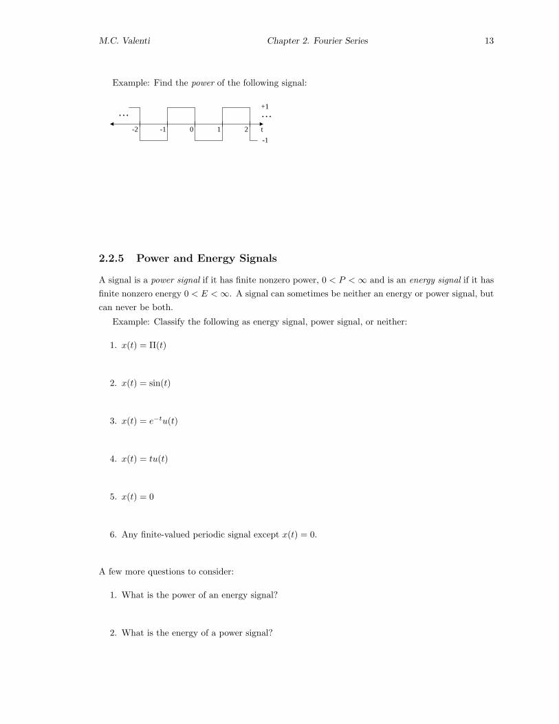
Example: Find the power of the following signal:

-2 -1 0 1 2 t

… …+1

-1

2.2.5 Power and Energy Signals

A signal is a power signal if it has finite nonzero power, 0 < P < ∞ and is an energy signal if it hasfinite nonzero energy 0 < E < ∞. A signal can sometimes be neither an energy or power signal, butcan never be both.

Example: Classify the following as energy signal, power signal, or neither:

1. x(t) = Π(t)

2. x(t) = sin(t)

3. x(t) = e−tu(t)

4. x(t) = tu(t)

5. x(t) = 0

6. Any finite-valued periodic signal except x(t) = 0.

A few more questions to consider:

1. What is the power of an energy signal?

2. What is the energy of a power signal?

14

2.3 Complex Exponentials

When we take the Fourier Series or Fourier Transform of a signal, the result is a complex-valuedsequence (the F.S. coefficients) or signal (the F.T. results in a function of frequency). Thus it isworthwhile to spend a few minutes reviewing the mathematics of complex numbers.

A complex number z can be represented in rectangular or Cartesian form:

z = x + jy (2.7)

where x and y are each real-valued numbers and j =√−1.

Alternatively, z can be represented in polar form:

z = rejθ (2.8)

where ejθ is a complex exponential and r is a real-valued number. We call r the magnitude and θ

the phase. Relating rectangular to polar coordinates:

x = r cos θ (2.9)

y = r sin θ (2.10)

r =√

x2 + y2 (2.11)

θ = 6 z (2.12)

2.3.1 Euler’s Equation

First, equate (2.7) and (2.8),

rejθ = x + jy. (2.13)

Next, substitute (2.9) and (2.10),

rejθ = r cos θ + jr sin θ (2.14)

Finally, divide both sides by r,

ejθ = cos θ + j sin θ. (2.15)

The above expression is known as Euler’s equation.From Euler’s equation we see that:

<{ejθ} = cos θ (2.16)

={ejθ} = sin θ (2.17)

What if the exponential is negative? Then:

e−jθ = cos(−θ) + j sin(−θ)

= cos θ − j sin θ (2.18)

since cos is an even function and sin is an odd function.


We can represent cos θ and sin θ in terms of complex exponentials:

cos θ =12

(ejθ + e−jθ

)(2.19)

sin θ =12j

(ejθ − e−jθ

)(2.20)

Proof:

2.3.2 Complex Conjugates

If z = x + jy = rejθ, then the complex conjugate of z is z∗ = x− jy = re−jθ.

What happens when we add complex conjugates? Consider z + z∗

What if we multiply complex conjugates? Consider (z)(z∗)

2.4 Rotating Phasors

One of the most basic periodic signals is the sinusoidal signal

x(t) = r cos(ω0t + θ), (2.21)

where ω0 = 2πfo is the angular frequency, r is the magnitude and θ is the phase of the sinusoidalsignal.

Another way to represent this sinusoid is as

x(t) = r<{

ej(ω0t+θ)}

= r<{ejθejω0t

}

= <{rejθejω0t

}

= <{zejω0t

}, (2.22)

16

where z = rejθ. The quantity zejω0t is called a rotating phasor, or just phasor for short. We canvisualize a phasor as being a vector of length r whose tip moves in a circle about the origin of thecomplex plane. The original sinusoid x(t) is then the projection of the phasor onto the real-axis.See the applet on the course webpage.

There is another way to use phasors to represent the sinusoidal signal without needing the <{·}operator. The idea is to use the property of complex conjugates that z + z∗ = 2<{z}. This impliesthat

<{z} =z + z∗

2. (2.23)

We can apply this property to the phasor representation of our sinusoidal signal:

x(t) = <{zejω0t

}

=12

[(zejω0t

)+

(zejω0t

)∗]

=12zejω0t +

12z∗e−jω0t

= aejω0t + a∗e−jω0t, (2.24)

where a = z/2. What (2.24) tells us is that we can represent a sinusoid as the sum of two phasorsrotating at the same speed, but in opposite directions.

2.5 Sum of Two Sinusoids

Suppose we have the sum of two sinusoids, one at twice the frequency of the other

x(t) = r1 cos(ω1t + θ1) + r2 cos(ω2t + θ2), (2.25)

where ω1 = ω0 and ω2 = 2ω0. Note that x(t) is periodic with an angular frequency of ω0. From(2.24), we can represent the signal as

x(t) = a1ejω1t + a∗1e

−jω1t + a2ejω2t + a∗2e

−jω2t

= a1ejω0t + a∗1e

−jω0t + a2ej2ω0t + a∗2e

−j2ω0t (2.26)

(2.27)

where ak = 12rkejθk , which implies that |ak| = rk/2 and 6 ak = θk.

If we let

a−1 = a∗1

a−2 = a∗2

a0 = 0 (2.28)

then we can represent x(t) more compactly as

x(t) =k=+2∑

k=−2

akejkωot (2.29)


2.6 Fourier Series

Now suppose that we have a signal which is the sum of more than just two sinusoids, with eachsinusoid having an angular frequency which is an integer multiple of ω0. Furthermore, the signalcould have a DC component, which is represented by a0. Then the signal can be represented as

x(t) = a0 +∞∑

k=1

rk cos(kω0t + θk) (2.30)

= a0 +∞∑

k=1

<{zkejkω0t

}, (2.31)

where zk = rkejθk . We can represent this signal as

x(t) =+∞∑

k=−∞akejkωot, (2.32)

where again ak = 12rkejθk and a−k = a∗k.

Theorem: Every periodic signal x(t) can be represented as a sum of weighted complex expo-nentials in the form given by equation (2.32). Furthermore, the coefficients ak can be computedusing

ak =1To

∫ to+To

to

x(t)e−jkωotdt (2.33)

Some notes:

• ωo = 2πfo = 2π/To is the fundamental angular frequency.

• The integral in (2.33) can be performed over any period of x(t).

• The Fourier Series coefficients ak are, in general, complex numbers.

• When k > 0, ak is also called the kth harmonic component.

• Since a−k = a∗k, |ak| and <{ak} are even functions of k, while 6 ak and ={ak} are odd functionsof k.

• ao is the DC component, and it is real-valued.

• You should compute ao as a separate case to avoid a divide by zero problem.

18

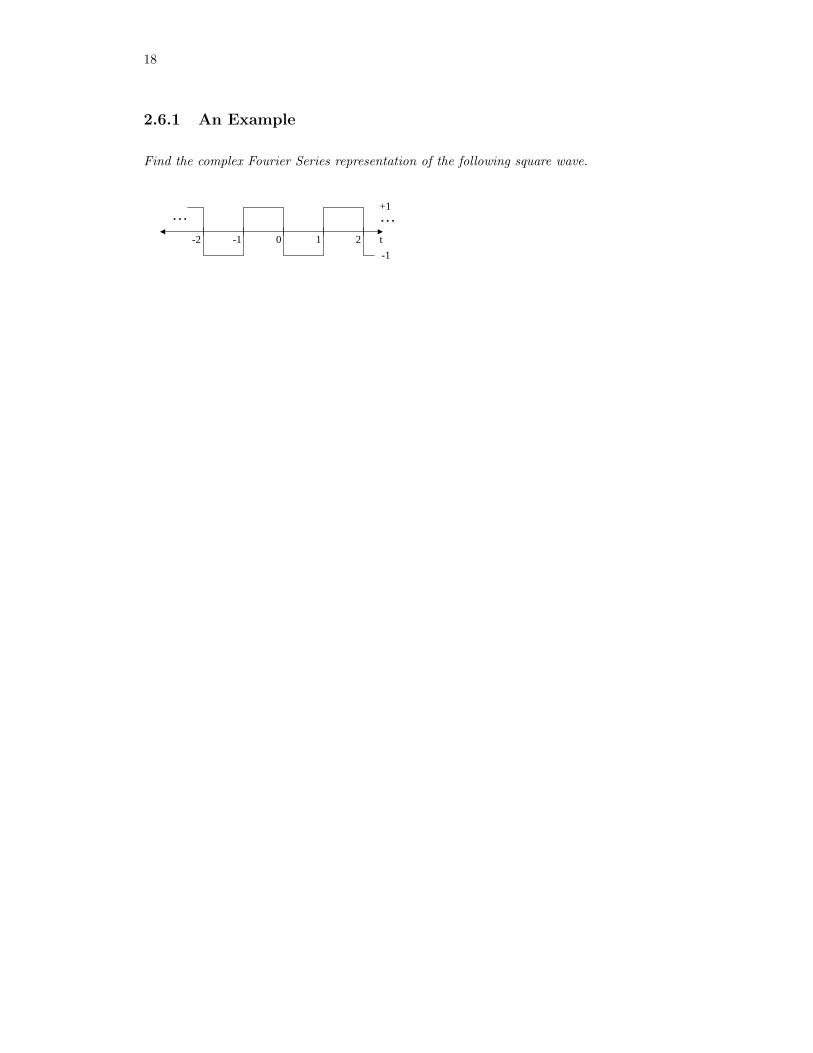
2.6.1 An Example

Find the complex Fourier Series representation of the following square wave.

-2 -1 0 1 2 t

… …+1

-1


2.7 Magnitude & Phase Spectra

We can depict the Fourier Series graphically by sketching the magnitude and phase of the complexcoefficients ak as a function of frequency. The Fourier Series tells us that the signal can be representedby a complex exponential located every kfo Hz, and that this exponential will be weighted by amountak. The magnitude spectra just represents the magnitudes of the coefficients Ak = |ak| with linesof height Ak located at kfo Hz. Likewise, the phase spectral shows the angle of the coefficientsθk = 6 ak. Sketch the magnitude and phase spectra for the example from the last page.

2.7.1 Trig Form of the Fourier Series

From (2.31), we can represent any periodic signal as

x(t) = a0 +∞∑

k=1

<{zkejkω0t

}. (2.34)

Let bk = <{zk} and ck = −={zk}, which implies that zk = bk − jck. Since ejkω0t = cos(kω0t) +j sin(kω0t), we have

x(t) = a0 +∞∑

k=1

<{[bk − jck] [cos(kω0t) + j sin(kω0t)]} (2.35)

= a0 +∞∑

k=1

<{[bk cos(kω0t) + ck sin(kω0t)]} (2.36)

The above is the trig form of the Fourier Series.How are the coefficients bk and ck found? Recall that ak = 1

2zk, so we can compute zk = 2ak,

zk = 2ak

=2To

∫ to+To

to

x(t)e−jkωotdt

=2To

∫ to+To

to

x(t) [cos(kω0t)− j sin(kω0t)]

=2To

∫ to+To

to

x(t) cos(kω0tdt− 2j

To

∫ to+To

to

x(t) sin(kω0t)dt (2.37)

Since bk = <{zk}, we get

bk =2To

∫ to+To

to

x(t) cos(kω0tdt (2.38)

20

and since ck = −={zk}, we get

ck =2To

∫ to+To

to

x(t) sin(kω0t)dt (2.39)

Note that the preferred form for the Fourier Series is the complex exponential Fourier Series givenby Equation (2.32). So you might wonder why we bother with the trig form? Well, it turns outfor some more complicated functions, it is more computationally efficient to first find the trig formcoefficients bk and ck, and then use those coefficients to determine ak.

Question: How can you find ak from bk and ck?

2.8 Parseval’s Theorem

Recall that the power of a periodic signal is found as:

P =1To

∫ to+To

to

|x(t)|2dt (2.40)

Since |x(t)|2 = x(t)x∗(t) this can be rewritten as:

P =1To

∫ to+To

to

x(t)x∗(t)dt (2.41)

Replace x∗(t) with its complex F.S. representation:

P =1To

∫ to+To

to

x(t)

(+∞∑

k=−∞akejkωot

)∗

dt

=1To

∫ to+To

to

x(t)∞∑

k=−∞a∗ke−jkωotdt (2.42)

Pull the summation to the outside and rearrange some terms:

P =∞∑

k=−∞a∗k

(1To

∫ to+To

to

x(t)e−jkωotdt

)

=∞∑

k=−∞a∗kak

=∞∑

k=−∞|ak|2 (2.43)

We see from the above equation that we can compute the power of the signal directly from theFourier Series coefficients.


Parseval’s Theorem: The power of a periodic signal x(t) can be computed from its FourierSeries coefficients using:

P =∞∑

k=−∞|ak|2

= a2o + 2

∞∑

k=1

|ak|2 (2.44)

Example: Use Parseval’s Theorem to compute the power of the square wave from Section 2.6.1.

22

2.9 Exercises

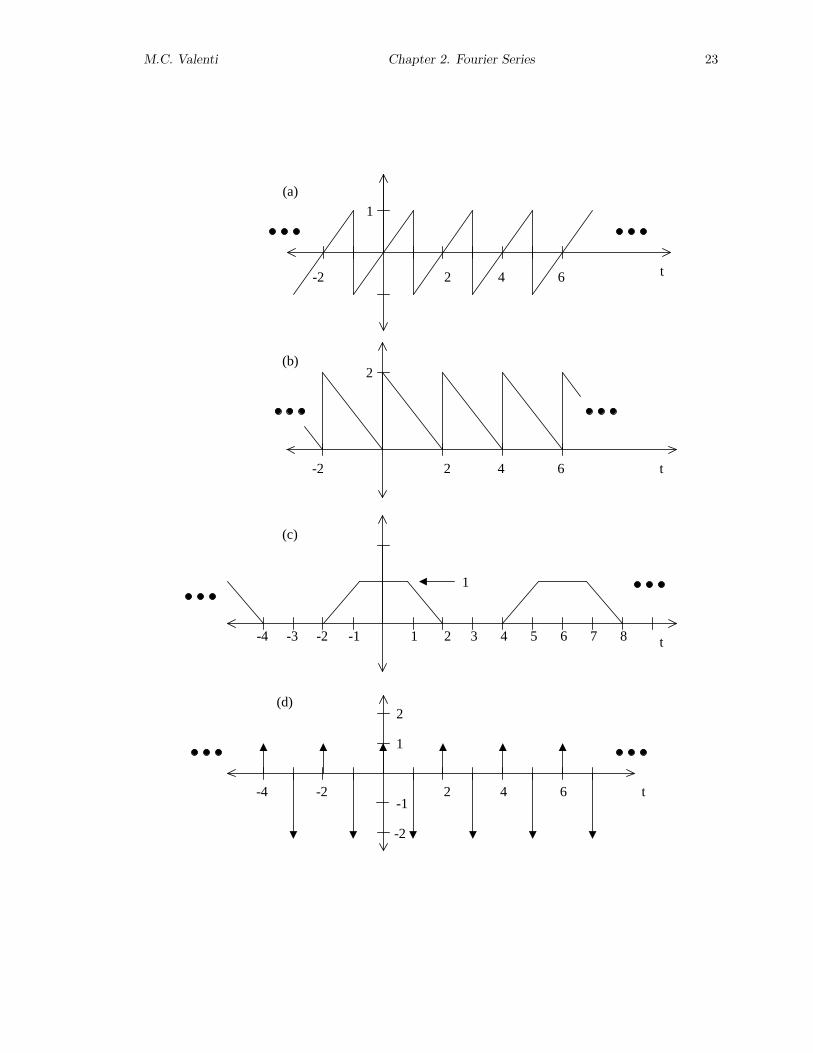
1. For periodic signal (a) shown on the next page

(a) Compute the power in the time domain (i.e. using equation 2.6).

(b) Calculate the complex Fourier Series coefficients ak. Try to get your answer into itssimplest form.

(c) Sketch the magnitude spectra |ak| for |k| ≤ 5.

(d) Use Parseval’s theorem to compute the power from the Fourier Series coefficients. Com-pare your answer to that of part (a).

Hint:n=∞∑n=1

1n2

=π2

6

2. Repeat 1 for periodic signal (b).

3. Repeat 1.a, 1.b, and 1.c for periodic signal (c). Hint: The book-keeping will be easier if you firstcompute the trig form coefficients bk and ck, and then use these to determine ak.

4. Repeat 1.b, and 1.c for periodic signal (d).

5. A periodic signal has the following complex Fourier Series coefficients:

ak =

1 for k = 0|k|e−jkπ/2 for 1 ≤ |k| ≤ 30 for |k| > 3

Compute the power of this signal. Give a numerical answer.

6. A periodic signal x(t) can be represented as:

x(t) =N∑

k=−N

kejk2πt

Determine the maximum value of the integer N such that the power of x(t) does not exceed20 Watts.


42 6-2

2

t

42 6-2

1

t

(a)

(b)

42 6-2

1

t

(c)

1 3 5 7 8-1-3-4

42 6-2 t-4

1

2

-1

-2

(d)

Chapter 3

The Fourier Transform

3.1 Definition of the Fourier Transform

If the signal x(t) is periodic, we can use the Fourier Series to obtain a frequency domain represen-tation. But what if x(t) is aperiodic? The key is to think of an aperiodic signal as being a periodicone with a very large period. In other words, an aperiodic signal is merely a periodic one withfundamental period To →∞.

When the period gets large, a few things occur:

• The limit of integration in (2.33) used to form the coefficients goes from −∞ to ∞.

• When we plot the magnitude spectra, we get a line every fo = 1/To Hz (this is why themagnitude spectra is sometimes called a line spectra). As To → ∞ these lines turn into acontinuous function of frequency.

• Because there are no longer discrete lines associated with particular frequencies, the summationin the Fourier Series representation (2.32) becomes an integral.

All these observations are captured in the Fourier Transform. The transform itself is similar tothe equation for generating Fourier Series coefficients, and is defined as follows:

X(w) =∫ ∞

−∞x(t)e−jωtdt (3.1)

The main difference is that we are now generating a continuous function of angular frequency (ratherthan a sequence of discrete coefficients), the limits of the integral are infinite, and the 1/To term infront of the integral is no longer there (since it would cause the function to be zero for all frequencies).

The inverse Fourier Transform is similar to the equation that expresses the signal as a functionof the Fourier Series coefficients, and is as follows:

x(t) =12π

∫ ∞

−∞X(ω)ejωtdω (3.2)

25

26

Note that the F.S. coefficients in (2.32) have been replaced with the Fourier Transform of the signal,which requires the summation to be replaced with an integral. The 1/(2π) term is a consequence ofrepresenting the transform in terms of angular frequency.

We can represent the Fourier Transform in terms of the true frequency (in Hz) rather than theangular frequency by using the following relations:

X(f) =∫ ∞

−∞x(t)e−j2πftdt

x(t) =∫ ∞

−∞X(f)ej2πftdf (3.3)

Both of these definitions of the Fourier Transform are used in practice, which is sometimes asource of confusion. Although you should be familiar with both representations (angular frequencyand true frequency), we will use the true frequency version (3.3) for the remainder of the text (sincethis is what is more commonly used in practice ... how often do you hear the broadcasting frequencyof an FM radio station expressed in rad/sec?).

Some other notation that is used:

X(f) = F {x(t)}x(t) = F−1 {X(f)}x(t) ⇔ X(f) (3.4)

3.2 Common F.T. Pairs and Properties

We will now derive several Fourier Transform pairs and several properties of the Fourier Transform.These pairs and properties are summarized in a table at the end of this book.

M.C. Valenti Chapter 3. Fourier Transform 27

3.2.1 F.T. Pair: Rectangular Pulse

Example: Let x(t) = Π(t/T ). Find X(f).

3.2.2 F.T. Pair: Complex Exponential

Example: Let x(t) = ejωot = ej2πfot. Find X(f).

28

3.2.3 F.T. Property: Linearity

Theorem: If x(t) ⇔ X(f) and y(t) ⇔ Y (f), then

ax(t) + by(t) ⇔ aX(f) + bY (f), (3.5)

where a and b are constants.

Proof:

3.2.4 F.T. Property: Periodic Signals

Let x(t) be a periodic signal with complex exponential Fourier Series coefficients ak. Find the F.T.of x(t) in terms of its F.S. coefficients.


3.2.5 F.T. Pair: Train of Impulses

Consider the train of dirac delta functions

x(t) =∞∑

k=−∞δ(t− kTo) (3.6)

Find X(f).

3.2.6 F.T. Property: Time Shifting

Theorem: If x(t) ⇔ X(f), then

x(t− to) ⇔ e−j2πftoX(f), (3.7)

where to is a constant time delay.Proof:

30

3.2.7 F.T. Property: Time Scaling


x (at) ⇔ 1|a|X

(f

a

), (3.8)

where a is a constant time-scaling factor.

Proof:


3.2.8 Example: Using F.T. Properties

Find the F.T. for the following signal:

x(t) = 3Π(

t− 22

)+ Π

(t

10

)(3.9)

32

3.2.9 F.T. Pair: Delta Function

Find the F.T. of x(t) = δ(t).

3.2.10 F.T. Pair: Constant

Find the F.T. of x(t) = K, where K is a constant.

3.2.11 F.T. Property: Duality

Theorem: Let the Fourier Transform of x(t) be X(f). Then the Fourier Transform of X(t) is x(−f).

Proof:

3.2.12 F.T. Pair: Sinc

Find the F.T. of x(t) = sinc(2Wt) where W is the “bandwidth” of x(t).


3.2.13 F.T. Pair: Cosine

Find the F.T. of x(t) = cos(ωot).

3.2.14 F.T. Property: Differentiation in Time


dn

dtnx(t) ⇔ (j2πf)nX(f) (3.10)

Proof:

3.2.15 F.T. Pair: Sine

Find the F.T. of x(t) = sin(ωot) by using the fact that

sin(ωot) = −(

1ωo

)d

dtcos(ωot)

34

3.2.16 F.T. Property: Integration


∫ t

−∞x(λ)dλ ⇔ 1

j2πfX(f) +

X(0)2

δ(f) (3.11)

Proof: Can be obtained by integration by parts when X(0) = 0. When X(0) 6= 0 then a limitingargument must be used.

3.2.17 F.T. Pair: Unit-step

Find the F.T. of x(t) = u(t) by using the fact that

u(t) =∫ t

−∞δ(t)dt


3.2.18 F.T. Property: Convolution

Theorem: If x(t) ⇔ X(f) and y(t) ⇔ Y (f) then

x(t) ∗ y(t) ⇔ X(f)Y (f) (3.12)

Proof:

3.2.19 F.T. Pair: Triangular Pulse

Find the F.T. of x(t) = Λ(t/T ) using the fact that

Π(t) ∗Π(t) = Λ(t)

or, more generally

Π(

t

T

)∗Π

(t

T

)= TΛ

(t

T

)

36

3.2.20 F.T. Pair: Train of pulses

Find the F.T. of the following train of pulses:

x(t) =∞∑−∞

Π(

t− kTo

τ

)(3.13)

By using

∞∑−∞

Π(

t− kTo

τ

)= Π

(t

τ

)∗∞∑−∞

δ (t− kTo) (3.14)

3.2.21 F.T. Property: Multiplication

Theorem: If x(t) ⇔ X(f) and Y (t) ⇔ Y (f) then

x(t)y(t) ⇔ X(f) ∗ Y (f) (3.15)

Proof: This is merely the dual of the convolution property.

3.2.22 F.T. Pair: Sinc-squared

Find the F.T. of x(t) = sinc2(2Wt)


3.2.23 F.T. Property: Frequency Shifting


ejωotx(t) ⇔ X(f − fo) (3.16)

where ωo = 2πfo

Proof: This is merely the dual of the time-delay property.

Example: Let x(t) = sinc(2t). Find the F.T. of y(t) = ejωotx(t) when ωo = 4π.

3.2.24 F.T. Pair: Decaying exponential

Find the F.T. of x(t) = e−atu(t)

3.2.25 F.T. Property: Differentiation in Frequency


tnx(t) ⇔ (−j2π)−n dn

dfnX(f) (3.17)

Proof: This is merely the dual of the differentiation in time property.

38

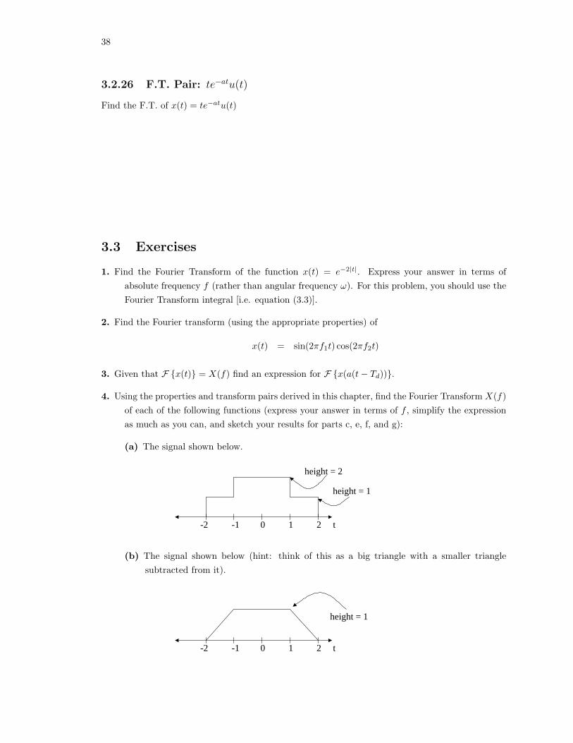
3.2.26 F.T. Pair: te−atu(t)

Find the F.T. of x(t) = te−atu(t)

3.3 Exercises

1. Find the Fourier Transform of the function x(t) = e−2|t|. Express your answer in terms ofabsolute frequency f (rather than angular frequency ω). For this problem, you should use theFourier Transform integral [i.e. equation (3.3)].

2. Find the Fourier transform (using the appropriate properties) of

x(t) = sin(2πf1t) cos(2πf2t)

3. Given that F {x(t)} = X(f) find an expression for F {x(a(t− Td))}.

4. Using the properties and transform pairs derived in this chapter, find the Fourier Transform X(f)of each of the following functions (express your answer in terms of f , simplify the expressionas much as you can, and sketch your results for parts c, e, f, and g):

(a) The signal shown below.

height = 1

-2 -1 0 1 2 t

height = 2

(b) The signal shown below (hint: think of this as a big triangle with a smaller trianglesubtracted from it).

height = 1

-2 -1 0 1 2 t


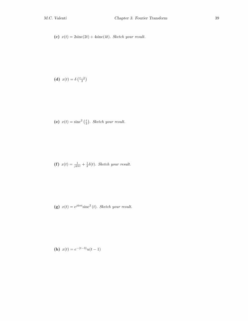
(c) x(t) = 2sinc(2t) + 4sinc(4t). Sketch your result.

(d) x(t) = δ(

t−32

)

(e) x(t) = sinc2(

t2

). Sketch your result.

(f) x(t) = 1j2πt + 1

2δ(t). Sketch your result.

(g) x(t) = ej6πtsinc2 (t). Sketch your result.

(h) x(t) = e−(t−3)u(t− 1)

40

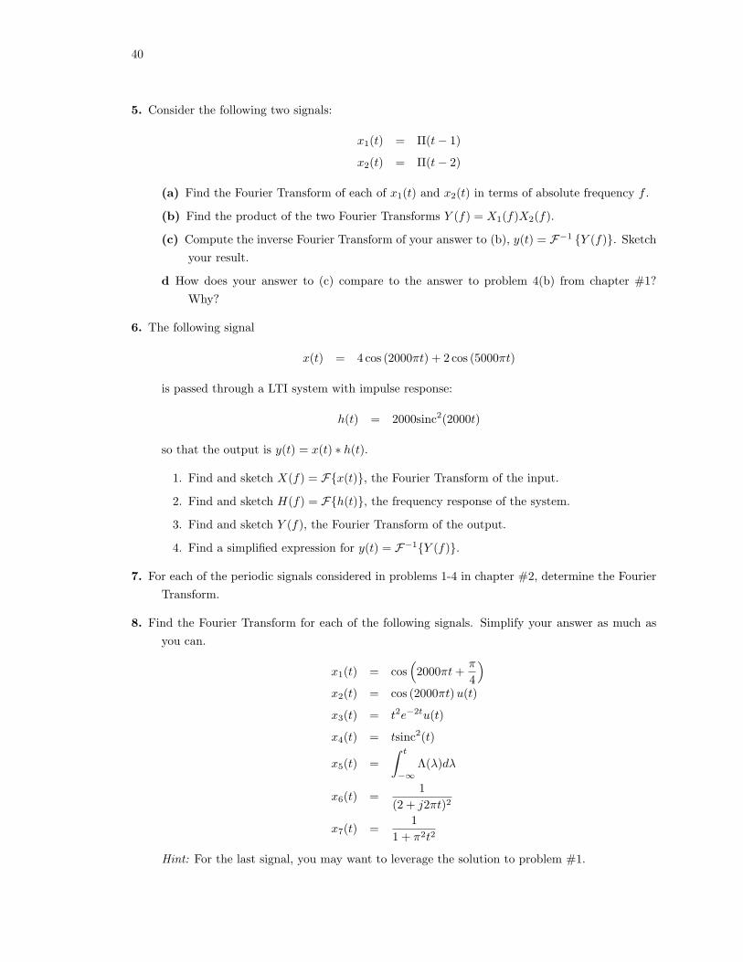
5. Consider the following two signals:

x1(t) = Π(t− 1)

x2(t) = Π(t− 2)

(a) Find the Fourier Transform of each of x1(t) and x2(t) in terms of absolute frequency f .

(b) Find the product of the two Fourier Transforms Y (f) = X1(f)X2(f).

(c) Compute the inverse Fourier Transform of your answer to (b), y(t) = F−1 {Y (f)}. Sketchyour result.

d How does your answer to (c) compare to the answer to problem 4(b) from chapter #1?Why?

6. The following signal

x(t) = 4 cos (2000πt) + 2 cos (5000πt)

is passed through a LTI system with impulse response:

h(t) = 2000sinc2(2000t)

so that the output is y(t) = x(t) ∗ h(t).

1. Find and sketch X(f) = F{x(t)}, the Fourier Transform of the input.

2. Find and sketch H(f) = F{h(t)}, the frequency response of the system.

3. Find and sketch Y (f), the Fourier Transform of the output.

4. Find a simplified expression for y(t) = F−1{Y (f)}.

7. For each of the periodic signals considered in problems 1-4 in chapter #2, determine the FourierTransform.

8. Find the Fourier Transform for each of the following signals. Simplify your answer as much asyou can.

x1(t) = cos(2000πt +

π

4

)

x2(t) = cos (2000πt) u(t)

x3(t) = t2e−2tu(t)

x4(t) = tsinc2(t)

x5(t) =∫ t

−∞Λ(λ)dλ

x6(t) =1

(2 + j2πt)2

x7(t) =1

1 + π2t2

Hint: For the last signal, you may want to leverage the solution to problem #1.


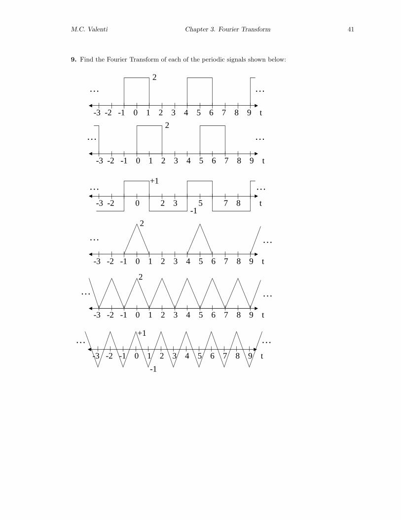
9. Find the Fourier Transform of each of the periodic signals shown below:

-3 -2 -1 0 1 2 3 4 5 6 7 8 9 t

2

… …

-3 -2 -1 0 1 2 3 4 5 6 7 8 9 t

2

… …

-3 -2 0 2 3 5 7 8 t

+1… …

-1

-3 -2 -1 0 1 2 3 4 5 6 7 8 9 t

2

… …

-3 -2 -1 0 1 2 3 4 5 6 7 8 9 t

2

… …

-3 -2 -1 0 1 2 3 4 5 6 7 8 9 t

… …+1

-1

Chapter 4

Filtering

4.1 Lowpass Signals and Filters

4.1.1 Ideal Lowpass Filter

An ideal lowpass filter hlpf (t) passes (with no attenuation or phase shift) all frequency componentswith absolute frequency |f | < W , where W is the bandwidth of the filter, and attenuates (completely)all frequency components with absolute frequency |f | > W .

Q: From the convolution theorem, what must the frequency response Hlpf (f) be?

Therefore, what is the impulse response hlpf (t)?

4.1.2 Lowpass Signals

A lowpass or baseband signal is a signal that can be passed through a lowpass filter (with finitebandwidth W ) without being distorted (i.e. its spectrum for all |f | > W is zero). The minimumvalue of W for which the signal is passed undistorted is the absolute bandwidth of the signal.

43

44

Q: For each of the following signals, determine if it is a baseband signal, and if so find its bandwidth:

x(t) = Π (t)

x(t) = Λ (t)

x(t) = sinc (4000t)

x(t) = 1 + cos(4000πt)

x(t) = e−tu(t)

4.1.3 Practical Lowpass Filters

It should be noted that an ideal lowpass filter is not attainable in practice.

Q: Why? (Consider the impulse response).

A practical lowpass filter has three regions:

Passband: All frequencies below Wp are passed with minimal distortion. Note however, that thepassband is not entirely flat. The passband ripple δ1 is the tolerance of the ripple in thepassband, i.e. in the passband, the frequency response satisfies 1 − δ1 ≤ |H(f)| ≤ 1 + δ1.Additionally, the passband may change the phase of the signal, although the phase responseof the filter will just be a linear function of frequency (which implies a constant time delay).

Stopband: Frequencies above Ws are almost completely attenuated (but not entirely). However, aswith the passband, the stopband is not entirely flat. The stopband ripple δ2 is the tolerance ofthe ripple in the stopband, i.e. in the stopband, the frequency response satisfies |H(f)| ≤ δ2.

Transition band/region: The frequency response of the filter cannot have a sharp transition, andthus must gradually fall from H(f) ≈ 1 at f = Wp to H(f) ≈ 0 at f = Ws. In the transitionband, 1− δ1 ≥ |H(f)| ≥ δ2. The center of the transition band is W , which is called the cutofffrequency.

M.C. Valenti Chapter 4. Filtering 45

Classes of practical filters.

Butterworth Filter: Can only specify cutoff frequency W and the filter “order” N . In MATLAB,use >>butter.

Chebyshev Filter: Can also specify the passband ripple δ1. In MATLAB, use >>cheby1 or>>cheby2.

Elliptic (Cauer) Filter: Can specify both the passband ripple δ1 and the stopband ripple δ2. InMATLAB, use >> ellip.

4.2 Highpass Signals and Filters

4.2.1 Ideal Highpass Filter

An ideal highpass filter hhpf (t) passes (with no attenuation or phase shift) all frequency compo-nents with absolute frequency |f | > W , where W is the cutoff frequency the filter, and attenuates(completely) all frequency components with absolute frequency |f | < W .

Q: From the convolution theorem, what must the frequency response Hhpf (f) be?

Therefore, what is the impulse response hhpf (t)?

4.2.2 Highpass Signals

A highpass signal is a signal that can be passed through a highpass filter (with finite nonzerocutoff frequency W ) without being distorted (i.e. its spectrum for |f | < W is zero). However, ifthe signal can also be a bandpass signal (defined below), it is not considered a highpass signal. Theabsolute bandwidth of highpass signals is infinite.

4.2.3 Practical Highpass Filters

Like practical lowpass filters, a practical highpass filter has a passband, stopband, and transitionregion. However, the stopband is lower in frequency than the passband, i.e Ws < Wp.

46

4.3 Bandpass Signals and Filters

4.3.1 Ideal Bandpass Filters

An ideal bandpass filter hbpf (t) passes (with no attenuation or phase shift) all frequency com-ponents with absolute frequency W1 < |f | < W2, where W1 is the lower cutoff frequency the filterad W2 is the upper cutoff frequency, and it attenuates (completely) all frequency components withabsolute frequency |f | < W1 or |f | > W2.

Q: From the convolution theorem, what must the frequency response Hbpf (f) be?

Therefore, what is the corresponding impulse response?

4.3.2 Bandpass Signals

A bandpass signal is a signal that can be passed through a bandpass filter (with finite nonzeroW1 and W2) without being distorted (i.e. its spectrum for |f | < W1 and |f | > W2 is zero). Theabsolute bandwidth of the bandpass signal is W = W2 −W1.

Q: For each of the following signals, determine if it is a bandpass signal, and if so find its bandwidth:

x(t) = cos(10000πt)sinc (1000t)

x(t) = 1 + cos(4000πt)

x(t) = cos(2000πt) + cos(4000πt)

4.3.3 Ideal Bandpass Filters

Ideal bandpass filters have a passband, two stopbands, and two transition bands

M.C. Valenti Chapter 4. Filtering 47

4.4 Example: Putting It All Together

For each of the following signals, determine if it is a baseband, highpass, or bandpass signal, and ifso, find its bandwidth:

x(t) = Π (1000t)

x(t) = sinc2(2t) cos(4πt)

x(t) = 1000sinc(1000t)

x(t) = 1000 cos(10000πt)sinc (1000t)

x(t) = 1 + cos(4000πt)

x(t) = cos(2000πt) + cos(4000πt)

x(t) = δ(t)− 1000sinc(1000t)

4.5 Exercises

1. Find and sketch the Fourier Transform for each of the following signals. Classify each as oneof the following: (a) Lowpass, (b) Highpass, (c) Bandpass, or (d) None-of-the-above. Notethat each signal should only belong to one category (the categories are mutually exclusive). Inaddition, state the bandwidth for each of these signals (even if infinite).

x1(t) = cos2 (1000πt)

x2(t) =∞∑

k=−∞δ(t− k)

x3(t) = 1000tsinc2(1000t)

x4(t) = cos(2000πt)u(t)

x5(t) = 4000sinc2(2000t) cos(2π(106)t

)

x6(t) = δ(t)− 2000sinc(2000t)

x7(t) = sin(1000πt) + cos(2000πt)

x8(t) = 4sinc (2t) cos(6πt)

48

2. The following baseband signal:

x(t) = 1 + 4 cos(2000πt) + 6 cos(4000πt) + 8 cos(6000πt)

is passed through an ideal filter with frequency response h(t). Find the output of the filter

when the filter is:

(a) An ideal lowpass filter with cutoff at 1500 Hz.

(b) An ideal highpass filter with cutoff at 2500 Hz.

(c) An ideal bandpass filter with passband between 1500 Hz and 2500 Hz.

3. Consider a linear time invariant (LTI) system with input x(t) and impulse response h(t). Theoutput is y(t) = x(t) ∗ h(t).

(a) If x(t) = Π(t) and y(t) = 5Λ(t), what must h(t) be?

(b) If x(t) = Π(t) and y(t) = Π(t− 1), what must h(t) be?

(c) If x(t) = Π(t) and y(t) = Π(t− 1) + Π(t + 1), what must h(t) be?

(d) If x(t) = Π(t) and y(t) = Π(

t2

), what must h(t) be?

(e) Now assume that x(t) = sinc(2000πt) and h(t) = sinc(1000πt). Find and sketch X(f),H(f), and Y (f). Find y(t).

4. Let the input x(t) of an ideal bandpass filter be:

x(t) = 1 + cos(20πt) + cos(40πt)

Determine and sketch the frequency response H(f) for the filter such that the output y(t) =x(t) ∗ h(t) is

y(t) = cos(20πt)

Chapter 5

Sampling

5.1 Sampling

Ideal or impulse sampling is the process of multiplying an arbitrary function x(t) by a train ofimpulses, i.e.

xs(t) = x(t)∞∑

k=−∞δ(t− kTs) (5.1)

where Ts is called the sample period, and fs = 1/Ts is the sample rate or sample frequency. Noticethat sampling turns a continuous-time signal into a discrete-time signal.

Example: Let x(t) = cos(2πt) and fs = 8. Sketch xs(t) for 0 ≤ t ≤ 2

5.1.1 Fourier Transform of a Sampled Signal

Let x(t) ⇔ X(f). Then the F.T. of the sampled signal xs(t) is

Xs(f) ⇔ fs

∞∑

k=−∞X(f − kfs) (5.2)

49

50

Proof: Find Xs(f) as a function of X(f).

5.1.2 Example: F.T. of Sampled Signal

Let x(t) = 1000sinc2(1000t). Sketch Xs(f) for the following sample rates:

1. fs = 4000

2. fs = 2000

M.C. Valenti Chapter 5. Sampling 51

3. fs = 1500

4. fs = 1000

5.2 Nyquist Sampling Theorem

5.2.1 Minimum fs

Question: If a baseband signal with bandwidth W is sampled at a rate of fs Hz, what is theminimum value of fs for which the spectral copies do not overlap?

52

5.2.2 Recovering x(t) from xs(t)

Question: Assume that a baseband signal is sampled with sufficiently high fs. How can the originalsignal x(t) be recovered from the sampled signal xs(t)?

5.2.3 Nyquist Sampling Theorem

The Nyquist Sampling Theorem states that if a signal x(t) has a finite bandwidth W , then itcan be uniquely represented by samples taken at intervals of Ts seconds, where fs = 1/Ts ≥ 2W .The value 2W is called the Nyquist rate.

5.2.4 Digital-to-analog Conversion

A corollary to the above theorem is that if a baseband signal x(t) with bandwidth W is sampled ata rate fs ≥ 2W , then the original signal x(t) can be recovered by first passing the sampled signalxs(t) through an ideal lowpass filter with cutoff between W and fs −W and then multiplying thefilter output by a factor of Ts.

Thus the frequency response of an ideal digital-to-analog converter (DAC) is:

H(f) = TsΠ(

f

fs

)(5.3)

The Π(·) term serves the purpose of filtering out all the spectral copies except the original (k = 0)copy, while the Ts term is required to make sure the reconstructed signal has the right amplitude[notice that the Ts term will cancel the fs term in Equation (5.2) since fs = 1/Ts).

5.2.5 Aliasing

If the signal is sampled at fs < 2W then frequency components above W will be “folded” down to alower frequency after the DAC process. When a high frequency component is translated to a lowerfrequency component, this process is called aliasing.


5.2.6 Example

Given the following signal:

x(t) = 1 + 2 cos(400πt) + 2 cos(800πt) (5.4)

1. What is the minimum value of fs for which the original signal can be recovered from thesampled signal without aliasing?

2. If the signal is sampled at fs = 700 Hz, then what would the signal at the output of an idealDAC be?

3. If the signal is sampled at fs = 600 Hz, then what would the signal at the output of an idealDAC be?

5.2.7 Anti-aliasing Filter

Many real-world signals are not bandlimited (i.e. they don’t have a finite bandwidth W ). For suchsignals, aliasing can be prevented by passing the signal through a lowpass filter prior to sampling.Such a filter is called an anti-aliasing filter and should have a cutoff of fs/2.

54

5.3 Exercises

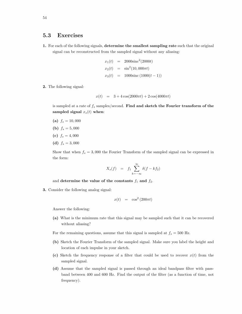
1. For each of the following signals, determine the smallest sampling rate such that the originalsignal can be reconstructed from the sampled signal without any aliasing:

x1(t) = 2000sinc2(2000t)

x2(t) = sin2(10, 000πt)

x3(t) = 1000sinc (1000(t− 1))

2. The following signal:

x(t) = 3 + 4 cos(2000πt) + 2 cos(4000πt)

is sampled at a rate of fs samples/second. Find and sketch the Fourier transform of the

sampled signal xs(t) when:

(a) fs = 10, 000

(b) fs = 5, 000

(c) fs = 4, 000

(d) fs = 3, 000

Show that when fs = 3, 000 the Fourier Transform of the sampled signal can be expressed inthe form:

Xs(f) = f1

∞∑

k=−∞δ(f − kf2)

and determine the value of the constants f1 and f2.

3. Consider the following analog signal:

x(t) = cos2 (200πt)

Answer the following:

(a) What is the minimum rate that this signal may be sampled such that it can be recoveredwithout aliasing?

For the remaining questions, assume that this signal is sampled at fs = 500 Hz.

(b) Sketch the Fourier Transform of the sampled signal. Make sure you label the height andlocation of each impulse in your sketch.

(c) Sketch the frequency response of a filter that could be used to recover x(t) from thesampled signal.

(d) Assume that the sampled signal is passed through an ideal bandpass filter with pass-band between 400 and 600 Hz. Find the output of the filter (as a function of time, notfrequency).


4. So far, we only considered sampling lowpass signals. However, some bandpass signals can also besampled and completely recovered, provided that they are sampled at a sufficiently high rate.Consider the following bandpass signal:

x(t) = 2 cos(800πt) + 2 cos(1000πt)

What is the bandwidth W of this signal? Suppose that the signal is sampled at exactly theNyquist rate, fs = 2W . Find and sketch the Fourier Transform of the sampled signal

xs(t) over the range −600 ≤ f ≤ 600. By looking at your sketch, suggest a way to recover theoriginal signal from the sampled signal. In particular, specify the frequency response of

an ideal digital-to-analog converter for this system.

Chapter 6

Communications

6.1 Communication Systems

• Communication systems transport an information bearing signal or message from a source toa destination over a communication channel.

• Most information bearing signals are lowpass signals:

1. Voice/music.

2. Video.

3. Data.

• Most communication channels act as bandpass filters:

1. Wireless: cellular, microwave, satellite, infrared.

2. Wired: coaxial cable, fiber-optics, twisted-pair (telephone lines, DSL).

• Thus, there is a mismatch between the source of information and the channel.

– The source is a lowpass signal but the channel is a bandpass filter.

– We know that lowpass signals cannot get through a bandpass filter.

– What we need to do is translate the lowpass message signal to a bandpass signal suitablefor delivery over the channel.

6.2 Modulation

Modulation is the process of translating a lowpass signal into a bandpass signal in such a way thatthe original lowpass signal can be recovered from the bandpass signal.

57

58

6.2.1 Types of Modulation

There are two main categories of modulation:

Linear: The lowpass (modulating) signal is multiplied by a high frequency carrier signal to formthe modulated signal. Amplitude Modulation (AM) is linear.

Angle: The lowpass (modulating) signal is used to vary the phase or frequency of a high frequencycarrier signal. Examples: Frequency Modulation (FM) and Phase Modulation (PM).

6.2.2 Simple Linear Modulation: DSB-SC

Let x(t) be a lowpass signal with bandwidth W . If we multiply x(t) by c(t) = cos(2πfct) we obtaina bandpass signal centered at fc, which is called the carrier frequency or center frequency. Thus themodulated signal is:

xm(t) = x(t) cos(2πfct)

This type of modulation is called Double Sideband Suppressed Carrier (DSB-SC). Sketch a diagramof a DSB-SC modulator here:

Example: Let x(t) = 100sinc2(100t) and the carrier frequency be fc = 1000 Hz. Find the FourierTransform of xm(t).

M.C. Valenti Chapter 6. Communications 59

6.2.3 Modulation Theorem

In general, if x(t) ⇔ X(f) then

x(t) cos(2πfct) ⇔ 12X(f − fc) +

12X(f + fc) (6.1)

Proof:

6.2.4 Minimum value of fc

In order to be able to recover x(t) from xm(t), then fc must be a minimum value. What is thisminimum value?

A (degenerate) example: Let x(t) = 100sinc2(100t) and the carrier frequency be fc = 50 Hz.Find the Fourier Transform of xm(t).

60

6.2.5 Demodulation

Given xm(t) (and assuming fc > W ) then how can x(t) be recovered (i.e. design a demodulator)?


6.3 DSB-LC

6.3.1 Motivation

A problem with DSB-SC is that it requires a coherent (or synchronous) receiver. With coherentreception, the phase of the receiver’s oscillator (i.e. the unit that generates cos(ωct)) must havethe same phase as the carrier of the received signal. In practice, this can be implemented with acircuit called a Phase Locked Loop (PLL). However, PLLs are expensive to build. Thus, we mightlike to design a system that uses a signal that can be detected noncoherently, i.e. without needinga phase-locked oscillator. Cheap receivers are essential in broadcasting systems, i.e. systems withthousands of receivers for every transmitter.

6.3.2 Definition of DSB-LC

A circuit called an envelope detector can be used to noncoherently detect a signal. However, for anenvelope detector to function properly, the modulating signal must be positive. We will see shortlythat this is because the envelope detector rectifies the negative parts of the modulating signal. Wecan guarantee that the modulating signal is positive by adding in a DC offset A to it, i.e. use A+x(t)instead of just x(t). Thus the modulated signal is:

xm(t) = (A + x(t)) cos(ωct) (6.2)

This type of signal is called Double Sideband Large Carrier (DSB-LC). Because this is the typeof modulation used by AM broadcast stations, it is often just called AM.

Sketch a block diagram of a DSB-LC transmitter:

What does a DSB-LC signal look like in the frequency domain?

62

6.3.3 Envelope Detector

An envelope detector is a simple circuit capable of following the positive envelope of the receivedsignal. Sketch the schematic of an envelope detector here:

In order to understand the operation of an envelope detector, it is helpful to sketch a typicalDSB-LC signal (in the time domain) and then show what the output of the detector would look like.

6.3.4 Modulation index

If the constant A is not high enough, then the modulating signal is not guaranteed to be positive.This causes the signal at the output of the envelope detector to be distorted, due to rectification ofthe negative parts. Let’s define a positive constant called the modulation index:

m =K

A(6.3)

=1A

max |x(t)| (6.4)

We can then rewrite our modulated signal as:

xm = (A + x(t)) cos(ωct) (6.5)

= A

(1 +

1A

x(t))

(6.6)

= A

(1 +

(K

A

)(x(t)K

))(6.7)

= A (1 + mx̃(t)) (6.8)

where x̃(t) = x(t)/K is the normalized1 version of x(t).From this equation, we see that the modulating signal is negative whenever mx̃(t) < −1. Since

max |x̃(t)| = 1, we assume that min x̃(t) = −1. This implies that m ≤ 1 in order to guarantee thatthe modulating signal is positive. When m > 1, we say that the signal is overmodulated, and anenvelope detector cannot be used to recover the original message x(t) without distortion.

1Normalized means that it is scaled so that max |x̃(t)| = 1.


6.4 Single Sideband

The two forms of DSB modulation that we have studied (DSB-SC and DSB-LC) get their namebecause both the positive and negative frequency components of the lowpass message signal aretranslated to a higher frequency. Thus there are two sidebands: a lower sideband that correspondsto the negative frequency components of the message signal, and an upper sideband that correspondsto the positive frequency components of the message. Thus, when we use DSB modulation, thebandwidth of the modulated signal is twice that of the message signal.

However, this doubling of bandwidth is wasteful. The two sidebands are redundant, in the sensethat one is the mirror image of the other. Thus, at least in theory, we really only need to transmiteither the upper or lower sideband. This is the principle behind single sideband modulation

(SSB). With SSB, only one or the other sideband (upper or lower) is transmitted. Note that thetransmitter and receiver circuitry for SSB is much more complicated that for DSB. However, SSBis more bandwidth efficient than DSB. SSB is commonly used in amateur radio bands.

6.5 Comparison of Linear Modulation

For each of the following, rank the three forms of modulation DSB-SC, DSB-LC, or SSB from “most”to “least”

Bandwidth efficiency:

Power efficiency (transmitter battery life):

Receiver complexity (cost):

64

6.6 Angle Modulation

With angle modulation, the message is encoded into the phase of the carrier, i.e.

xm(t) = A cos (ωct + θc(t))

= A cos (ωct + g[x(t)])

where the phase θc(t) = g[x(t)] is defined by a function g(t) of the message x(t). Depending on howg(t) is defined, the modulation can be either phase modulation (PM) or frequency modulation (FM).

6.6.1 Phase Modulation

With PM,

θc(t) = θo + kpx(t)

where kp is the phase sensitivity and θo is the initial phase. Without loss of generality, we mayassume that θo = 0, in which case the phase of the carrier is proportional to the message signal.Note that PM is not currently widely used.

6.6.2 Frequency Modulation

With FM, the information signal is used to vary the carrier frequency about the center value fc.Note that frequency is the derivative of phase. Thus if the modulated signal is expressed as:

xm(t) = A cos θ(t)

then the phase θ(t) is related to the message by

dθ(t)dt

= ωc + kfx(t)

where kf is the frequency sensitivity. Alternatively, we can think of phase as the integral of frequencyand thus the modulated signal is:

xm(t) = A cos(

ωct + kf

∫ t

−∞x(λ)dλ

)

Due to the existence of inexpensive equipment to produce and receive this type of signal, FM is themost popular type of analog modulation. Examples: FM radio, AMPS (analog) cell phones.

Spectrum of FM: Because the signal is embedded in the phase of the carrier, finding the FourierTransform of a FM signal with an arbitrary modulating signal is very difficult. However, we canfind the F.T. if we assume that the modulating signal is sinusoidal, e.g. if x(t) = cos(ωmt). But thisgets complicated and goes beyond the scope of this book.


6.7 Exercises

1. The following message signal

x(t) = 400sinc(200t)

is used to modulate a carrier. The resulting modulated waveform is:

xm(t) = 400sinc(200t) cos(2000πt)

(a) Sketch the Fourier Transform Xm(f) of the modulated signal.

(b) What kind of modulation is this? Be speficic (e.g. DSB-SC, DSB-LC, USSB, or LSSB).

(c) Design a receiver for this signal. The input of the receiver is xm(t) and the outputshould be identical to x(t). Make sure you accurately sketch the frequency response ofany filter(s) you use in your design.

2. Consider the system shown below:

cos(10πt)

x(t) IdealBPF

x1(t)

cos(6πt)

IdealLPF

x2(t) x4(t)x3(t)

Where the Fourier Transform of the input is:

X(f) = 4Λ(

f

2

)

The ideal bandpass filter (BPF) has a passband between 3 and 5 Hz, and the ideal lowpassfilter (LPF) has a cutoff at 2 Hz. Carefully sketch the Fourier Transform of signals

x1(t), x2(t), x3(t), and x4(t). Is the output x4(t) of this system the same as the input

x(t)?

3. Consider a DSB-SC system where the Fourier Transform of the message signal x(t) is:

X(f) = 2Π(

f

20

)

and the carrier frequency is fc = 30 Hz.

(a) Find and sketch the Fourier Transform of the modulated signal xm(t).

(b) Assume that the receiver is identical to the coherent receiver studied in class, only theoscillator does not have the exact same frequency as the carrier. More specifically, assumethat the receiver’s oscillator frequency is fo = 29 Hz. Find and carefully sketch the

Fourier Transform of the output of this receiver. Is the output of the receiver

the same as the input to the transmitter?

66

4. Consider a DSB-LC system where the message signal is:

x(t) = cos(2πt) + cos(6πt)

and the modulated signal is:

xm(t) = [A + x(t)] cos(10πt)

(a) What is the minimum value of the constant A for which an envelope detector canbe used to recover the message signal x(t) from the modulated signal xm(t) withoutdistortion?

(b) Using the value for A that you found in part A, find and sketch the Fourier Transform

of the modulated signal xm(t).

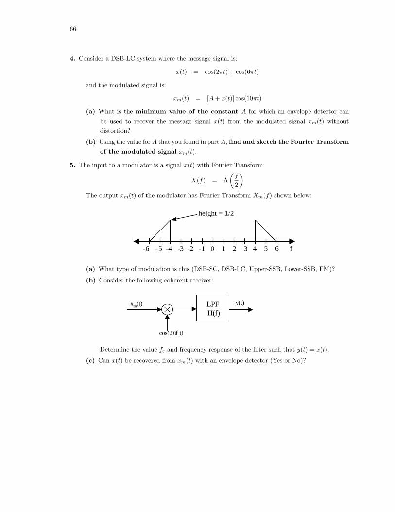
5. The input to a modulator is a signal x(t) with Fourier Transform

X(f) = Λ(

f

2

)

The output xm(t) of the modulator has Fourier Transform Xm(f) shown below:

height = 1/2

-6 –5 -4 -3 -2 -1 0 1 2 3 4 5 6 f

(a) What type of modulation is this (DSB-SC, DSB-LC, Upper-SSB, Lower-SSB, FM)?

(b) Consider the following coherent receiver:

LPFH(f)

y(t)

cos(2πfct)

xm(t)

Determine the value fc and frequency response of the filter such that y(t) = x(t).

(c) Can x(t) be recovered from xm(t) with an envelope detector (Yes or No)?


6. Consider the following system:

BPFHBPF(f)

LPFHLPF(f)

∑∞−∞=

−k

skTt )(δ)2cos( tfcπ

x(t)=2cos(20πt) x1(t) x2(t) x3(t) y(t)

HBPF(f) Height = 1 HLPF(f) Height = A

where the frequency response of the BPF and LPF are as shown.

(a) If fs = 1/Ts = 50 Hz, determine values for the parameters fc and A such that y(t) = x(t).

(b) For your choice of fc, what type of modulation is x2(t)?

Chapter 7

Probability

7.1 Prelude: The Monte Hall Puzzler

You have been selected to be a contestant on the TV game show ”Let’s Make A Deal”. The rulesof the game are as follows:

• There are three closed doors. Behind one of the doors are the keys to a new car. Behind eachof the other two doors is a box of Rice-A-Roni (the San Francisco treat).

• You begin the game by selecting one of the three doors. This door remains closed.

• Once you select a door, the host (Monty Hall) will open up one of the other two doors revealing... a box of Rice-A-Roni.

• You must choose between keeping the door that you originally selected or switching to theother closed door. The door that you chose is then opened and you are allowed to keep theprize that is behind it (and in the case of the keys, you get ownership of the car).

Answer the following.

1. If you want to maximize your chances of winning the car, should you:

(a) Keep the door you originally selected.

(b) Switch to the other door.

(c) Randomly choose between the two doors.

You may assume that Monty Hall knows which door has the keys behind it and that he doesn’twant you to win the car.

2. What is the probability of winning the car if you stay with your original choice?

3. What is the probability if you switch your choice?

4. What is the probability if you choose between the two closed doors at random?

69

70

7.2 Random Signals

Up until now, we have only considered deterministic signals, i.e. signals whose parameters arenon-random. However, in most practical systems, the signals of interest are unknown. For instance,in a communication system, the message signal is not known and the channel noise is not known.Unknown signals can be modelled, with the aid of probability theory, as random signals. Thechapter after this one is on random signals. But first, we need to start with a review of probabilityand random variables.

7.3 Key Terms Related to Probability Theory

7.3.1 Random Experiment

A random experiment is an experiment that has an unpredictable outcome, even if repeatedunder the same conditions. Examples include: A coin toss, a die roll, measuring the exact voltageof a waveform. Give some other examples of random experiments.

7.3.2 Outcome

An outcome is the result of the random experiment. Example: For a coin toss there are twopossible outcomes (heads or tails). Note that the outcomes of a random experiment are mutuallyexclusive (i.e. you can’t toss heads and tails at the same time with a single coin) and that theyaren’t necessarily numbers (heads and tails are not numbers, are they?).

7.3.3 Sample Space

The sample space is the set S of all outcomes. For examples, we write the sample space of a cointoss as:

S = {heads, tails}.

7.3.4 Random Variable

The outcomes of a random experiment are not necessarily represented by a numerical value (i.e. cointoss). A random variable (RV) is a number that describes the outcome of a random experiment.Example: for a coin toss, define a random variable X, where:

X =

{0 if “tails”1 if “heads”

M.C. Valenti Chapter 7. Probability 71

7.4 Cumulative Distribution Function

7.4.1 Definition

The Cumulative Distribution Function (CDF) of a random variable X is defined by:

FX(a) = P [X ≤ a]

where P [E] denotes the probability of event E. In words, the CDF is a function of a that tells usthe probability that the random variable X is less than or equal to a.

7.4.2 Example

A “fair” coin toss is represented by the random variable

X =


Find and sketch the CDF for this RV.

7.4.3 Properties

All valid CDFs have the following properties:

1. FX(a) is a nondecreasing function of a. That is, as a increases, Fx(a) cannot decrease.

2. FX(−∞) = 0.

3. FX(∞) = 1.

4. P [a < X ≤ b] = FX(b)− FX(a).

72

7.5 Probability Density Function

7.5.1 Definition

The probability density function (pdf) of a random variable X is defined by:

fx(x) =d

daFX(a)

∣∣∣∣a=x

Simply put, the pdf is the derivative of the CDF.

7.5.2 Example

Find the pdf for our example (fair coin toss).

7.5.3 Properties

All valid pdfs have the following properties:

1. The probability that the RV takes on a value within the range (a, b] is found by integratingthe pdf over that range:

P [a < X ≤ b] =∫ b

a

fX(x)dx

2. fX ≥ 0, i.e. the pdf is nonnegative.

3. The pdf integrates to one, i.e.:

∫ ∞

−∞fX(x)dx = 1


7.5.4 Another example

Consider a uniform RV that takes on values in the range (−1, +1) with equal probability. The pdfof this RV is:

fX(x) = cΠ(x

2

)

First, find the value of c such that this is a valid pdf.

Next, compute the following probabilities:

1. P [−1 < X ≤ 0]

2. P [|X| < 1/4]

3. P [X < 1/2]

74

7.5.5 Bernoulli Random Variable

The most basic discrete random variable is the Bernouilli random variable. Consider an unfaircoin that lands on heads with probability p. Assign a random variable X according to:

X =


The pdf of this random variable is:

fX(x) = (1− p)δ(x) + pδ(x− 1)

7.5.6 Uniform Random Variable

One of the most basic continuous random variable is the uniform random variable. A uniformrandom variable takes on values over the continuous range (a, b) with equal probability. The pdf isas follows:

fX(x) =1

b− aΠ

(x−m

b− a

)

where

m =b + a

2

7.6 Independence

Two random variables, X and Y , are independent if the random experiments that generate the tworandom variables are independent. In other words, if the outcome of the experiment that produces X

has no influence on the outcome of the experiment that produces Y , then X and Y are independent.

7.6.1 Independent and Identically Distributed

Two random variables, X and Y , are said to be “independent and identically distributed” if theyare independent and have the same pdf, i.e. fY (λ) = fX(λ).

7.6.2 Sums of Independent Random Variables

Theorem: Let Z = X + Y , where X and Y are independent. Then the pdf of Z is found byconvolving the pdfs of X and Y :

fZ(z) = fX(z) ∗ fY (z)


7.6.3 Example #1

Let X and Y be i.i.d. random variables that are each uniform over (−0.5, 0.5). Find the pdf ofZ = X + Y .

7.6.4 Example #2

Let X and Y be two i.i.d. Bernoulli random. Find the pdf of Z = X + Y .

7.6.5 A Generalization of the Theorem

Let X1, X2, ..., XN be a set of N independent random variables. Then the pdf of Y =N∑

n=1

Xn is

fY (y) = fX1(y) ∗ fX2(y) ∗ ... ∗ fXN(y)

7.6.6 Binomial Random Variables

Let X1, X2, ...XN be a set of i.i.d. Bernoulli random variables, then the pdf of Y =N∑

n=1

Xn is

fY (y) = fX1(y) ∗ fX2(y) ∗ ... ∗ fXN (y)

= [qδ(y) + pδ(y − 1)] ∗ [qδ(y) + pδ(y − 1)] ∗ ... ∗ [qδ(y) + pδ(y − 1)]

=N∑

k=0

(N

k

)pkqn−kδ(y − k)

where q = 1− p and

(N

k

)is called the binomial coefficient, defined by:

(n

k

)=

n!k!(n− k)!

76

7.6.7 Example #1

A fair coin is tossed 5 times. Find the probability that 2 or fewer heads were tossed.

7.6.8 Example #2

Data is transmitted over a noisy channel with bit error probability p = 0.001. Find the probabilitythat there is more than one bit error in a byte of received data.

7.7 Expectation

The expected value or mean of a random variable X is defined by:

mX = E[X] (7.1)

=∫ ∞

−∞xfX(x)dx (7.2)

7.7.1 Example #1

Find the mean of an arbitrary uniform random variable.


7.7.2 Example #2

Find the mean of an arbitrary Bernoulli random variable.

7.7.3 Moments

The n-th moment of a random variable X is defined by:

E[Xn] =∫ ∞

−∞xnfX(x)dx (7.3)

Note that the mean is the first moment.

7.7.4 Example #1

Find the second moment of an arbitrary uniform random variable.

7.7.5 Example #2

Find the second moment of an arbitrary Bernoulli random variable.

7.7.6 Variance

The variance of a random variable X is defined by:

σ2X = E[(X −mX)2] (7.4)

=∫ ∞

−∞(x−mX)2fX(x)dx (7.5)

78

7.7.7 Relationship Between Variance and First Two Moments

Variance is a function of the first and second moments:

σ2X = E[X2]−m2

X

Proof:

7.7.8 Example #1

Find the variance of an arbitrary uniform random variable.

7.7.9 Example #2

Find the variance of an arbitrary Bernoulli random variable.


7.8 Gaussian RV’s

7.8.1 The Central Limit Theorem

Let X1, X2, ..., XN be a set of N i.i.d. continuous random variables (e.g. uniform). Then the pdf of

Y =N∑

n=1

Xn is

fY (y) = fX1(y) ∗ fX2(y) ∗ ... ∗ fXN(y)

As N →∞, Y will have a Gaussian distribution:

fY (y) =1

σ√

2πexp

{−(y −m)2

2σ2

}

where m is the mean of Y and σ2 is the variance of Y .

This is called the Cental Limit Theorem and justifies the use of Gaussian RVs for manyengineering applications, e.g. measurement error, receiver noise, interference, etc.

A shorthand notation that is often used is X ∼ η(m, σ2

). This tells us that X has a normal

(i.e. Gaussian) distribution with mean m and variance σ2.

7.8.2 Properties of Gaussian RVs

Gaussian RVs have the following properties:

1. A Gaussian RV is completely described by its mean and variance.

2. The sum of 2 Gaussian RVs is also Gaussian.

3. If X and Y are Gaussian and E[XY ] = E[X]E[Y ], then X and Y are independent.

4. The pdf of a Gaussian RV is symmetric about its mean, and thus P [Y ≤ m] = P [Y > m] = 1/2.

80

7.8.3 Example: Applying the properties of Gaussian RVs

X1 and X2 are i.i.d. η(2, 3). What is the pdf of Y = X1 + X2?

What is the median of Y ?

If E[X1X2] = 4, then are X1 and X2 independent?

7.8.4 Computing the CDF of Gaussian RVs

Let X be Gaussian, then its CDF is:

FX(a) =∫ a

−∞fX(x)dx

where

erf(z) =2√π

∫ z

0

e−x2dx

is called the error function. You can compute this in matlab by using the erf command.


7.8.5 Area Under the Tail of a Gaussian RV

The complement of the CDF is the “area under the tail”.

∫ ∞

a

fX(x)dx = 1− FX(a)

where

erfc(z) = 1− erfc(z)

is called the complementary error function, which can be computed in matlab using erfc.

The area under the tail can also be put in terms of the Q-function:

Q(z) =1√2π

∫ ∞

z

e−x2/2dx

=12erfc

(z√2

)

In particular,

1− FX(a) = Q

(a−m

σ

)

7.8.6 Properties of the Q-function

The Q-function has the following properties:

1. Q(0) = 1/2.

2. Q(∞) = 0.

3. Q(−z) = 1−Q(z).

Let X ∼ η(m, σ2), then

FX(a) = Q

(m− a

σ

)

82

You can download a matlab script for computing the Q-function from the course web-page, or usethe following Q-function table:

z Q(z) z Q(z) z Q(z) z Q(z)

0.0 0.50000 1.0 0.15866 2.0 0.02275 3.0 0.001350.1 0.46017 1.1 0.13567 2.1 0.01786 3.1 0.000970.2 0.42074 1.2 0.11507 2.2 0.01390 3.2 0.000690.3 0.38209 1.3 0.09680 2.3 0.01072 3.3 0.000480.4 0.34458 1.4 0.08076 2.4 0.00820 3.4 0.000340.5 0.30854 1.5 0.06681 2.5 0.00621 3.5 0.000230.6 0.27425 1.6 0.05480 2.6 0.00466 3.6 0.000160.7 0.24196 1.7 0.04457 2.7 0.00347 3.7 0.000110.8 0.21186 1.8 0.03593 2.8 0.00256 3.8 0.000070.9 0.18406 1.9 0.02872 2.9 0.00187 3.9 0.00005

7.8.7 Examples

Let X ∼ η(0, 1). Compute the following probabilities:

1. P [X > 2]

2. P [X ≤ 2]

3. P [X > −1]

4. P [X ≤ −1]

Let X ∼ η(1, 4). Compute the following:

1. P [X > 2]

2. P [X ≤ 2]

3. P [X > −5]

4. P [X ≤ −5]


7.9 Exercises

1. For a probability density function (pdf) to be valid, the follow two properties must be satisfied:

i. The pdf is a nonnegative function (i.e. fX(x) ≥ 0, ∀x).

ii. The pdf integrates to one.

Determine whether or not each of the following pdfs is valid:

(a): fX(x) =1π

(1

1 + x2

)

(b): fX(x) =

{|x|, |x| < 10, otherwise

(c): fX(x) =

{16 (8− x), 4 ≤ x ≤ 100, otherwise

(d): fX(x) =∞∑

k=0

34

(14

)k

δ(x− k)

Hint:∞∑

k=0

rk =1

1− rif |r| < 1

2. A random variable X1 describes the outcome of a fair die roll.

(a) What is the sample space S of the random experiment used to produce X1?

(b) Find the CDF of X1.

(c) Find the pdf of X1.

(d) Find the probability that 3 < X1 ≤ 5.

(e) Let X2 be another random variable that also describes the outcome of a fair die roll. Letthe two die rolls that produce X1 and X2 be independent. Next, define a random variableY = X1 +X2 which describes the outcome when the pair of dice are rolled. Repeat parts2.a through 2.d, but answer these for Y rather than for X1.

3. A random variable X is uniform over the region (−1, 3).

(a) Write an expression for the pdf in terms of the Π(·) function and sketch the pdf.

(b) Determine P [X ≤ 0]

(c) Determine P [X > 1.5]

(d) Determine P [−0.5 < X ≤ 2]

84

4. A random variable X1 has pdf:

fX1(x) = ce−2xu(x)

where u(x) is the unit step function and c is a positive constant.

(a) Determine the value of the constant c required for this to be a valid pdf.

(b) Determine the median value of X1, i.e. the exact value of X1 for which the randomvariable is just as likely to be greater than this value as it is to be lower than it.

(c) Let X2 be a second random variable that is independent from X1 but has the same pdf.Let Y = X1 + X2. Find the pdf of Y (hint: you may use your FT table to help with thisproblem).

5. A random variable X has pdf:

fX(x) =

{332 (−x2 + 8x− 12), xo ≤ x ≤ 60, otherwise

(a) Determine the value of xo that makes fX(x) a valid pdf.

(b) Find the mean of X, i.e. E[X].

(c) Find the second moment of X, i.e. E[X2].

(d) Find the variance of X.

(e) Find P [X ≤ 4].

6. Let X1, X2, and X3 be independent and identically distributed (i.i.d.) random variables withpdf

fX(x) =12δ(x) +

12δ(x− 1)

and let Y1 and Y2 be i.i.d. random variables with pdf

fY (y) = Π(y).

The Xi’s are independent from the Yj ’s. Further define Z = X1 + Y1. Compute the followingquantities (give a numerical value for each):

(a) P [X1 ≤ 0]

(b) P [X1 + X2 > 0]

(c) P [X1 + X2 + X3 > 1]

(d) P [Y1 ≤ 0]

(e) P[|Y1 + Y2| > 1

2

]

(f) P [Z ≤ 0]

(g) The mean of Z

(h) The variance of Z


7. A digital communication systems transmits packets of data in frames of 16 bits. The system usesan error correction code that is capable of correcting up to 2 bit errors per frame. In otherwords, if the frame is received with 2 or fewer errors it can be correctly decoded, but if theframe is received with more than 2 errors it will be incorrectly decoded. If the probabilitythat any one bit is in error is p = 0.01, then find the probability that the frame is incorrectlydecoded.

8. A random variable X has a Gaussian distribution with mean µ and variance σ2. Find theprobability that:

(a) |X − µ| < σ.

(b) |X − µ| < 2σ.

(c) |X − µ| < 3σ.

9. Let X1 and X2 be a pair of independent and identically distributed random variables, each witha Gaussian pdf with a mean of 1 and variance of 4. Let Y be a Gaussian random variable thatis created by:

Y = X1 + 3X2

(a) Determine P [X1 ≤ 0].

(b) Determine P [X2 ≤ 3].

(c) Determine P [Y ≤ 4].

(d) Determine P [Y ≤ −8].

10. X1 and X2 are a pair of Gaussian random variables with the following properties:

• X1 has a mean of zero and variance of 4.

• X2 has a mean of 4 and a variance of 16.

• E[X1X2] = 0.

Compute the following probabilities (give numerical answers to five decimal places):

1. P [X1 ≤ 2]

2. P [|X1| ≤ 4]

3. P [X2 ≤ 2]

4. P [|X2| ≤ 6]

5. P [(X1 + X2) ≤ 4]

6. P [(X1 + X2) ≤ 8.47]

11. Error control codes are often used to improve the performance of practical digital communica-tions (e.g. cellular phones) and storage systems (e.g. compact discs, hard drives, and DVDs).Assume that a code can correct t=6 or fewer errors in a block of n coded bits. Also assumethat each code bit has an error probability of p = 0.001. What is the largest value of n forwhich the probability that the code word is incorrectly decoded is no more than Pe = 10−6?Hint: You might want to use MATLAB to help you arrive at your answer.

86

12. (Problem 2.10 from M.P. Fitz, Analog Communication Theory) A random variable X has pdfgiven by

fX(x) =

0 x < 0K1 0 ≤ x < 1K2 1 ≤ x < 20 x ≥ 2

(a) If the mean of X is 1.2, find K1 and K2.

(b) Find the variance of X using the value of K1 and K2 computed in (a).

(c) Find the probability that X ≤ 1.5 using the value of K1 and K2 computed in (a).

13. (This is Problem 2.11 of Fitz) In communications, the phase shift induced by propagationbetween transmitter and receiver, Φ is often modeled as a random variable. A common modelis to have

fΦ(φ) =

{12π for −π ≤ φ ≤ π

0 elsewhere

This is a uniformly distributed random variable.

(a) Find the CDF of Φ.

(b) Find the mean and variance of Φ.

(c) A particular communication system will work reasonable well if the estimated phase Φ̂ iswithin 30o of the true value of Φ. If you implement a receiver with Φ̂ = 0, what is theprobability that the communication system will work?

(d) Assume that if you move the receiver’s antenna, you randomly change the propagationdelay and obtain an independent phase shift. What is the probability that the systemwill work in at least one out of two antenna locations?

(e) How many antenna locations would you have to try to ensure a 90% chance of getting thesystem to work?

14. A biometrics system is used to determine whether or not a certain subject is ”Nicholas”. Thesystem scans the fingerprint of the subject and compares the fingerprint against a storedtemplate for Nicholas. Based on how close the scanned fingerprint is to the template, itgenerates a matching score X, which is a random variable. The system declares that theindividual is Nicholas if X > 1, otherwise it declares that the individual is not Nicholas. If thesubject is Nicholas, then X is Gaussian with mean m = 3 and variance σ2 = 4. Otherwise, ifthe subject is somebody else, then X is uniformly distributed over the range −b < X < b.

(a) What is the probability that the system makes a mistake when it scans Nicholas’s finger-print (i.e. it thinks that the subject is not Nicholas, even though it actually is)?

(b) Suppose that the system makes a mistake 10% of the time when the subject is not Nicholas(i.e. it declares that the subject is Nicholas, even though it is not). What is the numericalvalue of b in this case?

Chapter 8

Random Processes

8.1 Random Variables versus Random Processes

Recall our definition of a random variable: “A random variable (RV) is a number that describesthe outcome of a random experiment”.

The definition of a random process is very similar: “A random process (RP) is a function oftime (or signal) that describes the outcome of a random experiment.

For instance, let the random experiment be a coin toss and then define a random process as:

x(t) =

{sin(t) if “tails”cos(t) if “heads”

Note that a random process evaluated at a particular instance in time is a random variable, forinstance let’s evaluate (or sample) this random process at time t = 0, then we get:

x(0) =

{sin(0) = 0 if “tails”cos(0) = 1 if “heads”

which is a random variable.

8.2 Describing a Random Process

Recall that a random variable can be described in terms of its mean and variance. Since a randomvariable is a number, the mean and variance is also a number. Likewise, we can describe a randomprocess in terms of its mean and variance, only now these two become functions. More specifically,we can use the mean and the autocorrelation function.

8.2.1 Mean

The mean of a random process is defined as mx(t) = E[x(t)]. In general, the mean may be a functionof time. However, for some processes it turns out that the mean is a constant.

87

88

In general it is difficult to compute the mean because the pdf itself could change over time.However, many random processes can be expressed as a function of a random variable. In this case,it is actually quite easy to find the mean of the random process.

Example: Consider the random process x(t) = cos(2πt+ θ) where θ is a random variable whichis uniformly distributed over the range (0, 2π). Compute the mean of x(t).

8.2.2 Autocorrelation Function

Since the mean of a RP can be a function of time, we would expect the same to be true for thevariance of the RP. Thus, we could define the variance of a RP as being σ2(t) = E[(x(t)−mX(t))2].However, for random processes it is more common to instead use a function called the autocorrelationfunction (ACF) which is defined as follows:

Rx(t1, t2) = E[x(t1)x(t2)]

Note that the ACF is actually a function of two times, and in that sense is actually more generalthan the variance (which would only be a function of just one time). Because it is a function of twotimes, the ACF tells us how the RP changes over time.

Example: Determine the ACF for x(t) = cos(2πt + θ), where θ ∼ U(0, 2π).

M.C. Valenti Chapter 8. Random Processes 89

8.2.3 Stationarity

A random process is said to be wide sense stationary (WSS) if:

1. The mean is a constant

mx(t) = mx

2. The ACF is a function of time difference only

Rx(t1, t2) = Rx(τ)

where τ = t2 − t1

Example: Is x(t) = cos(2πt + θ) WSS when θ ∼ U(0, 2π)?

8.2.4 Power Spectral Density

So what does knowing that a RP is WSS “buy” us? Well, actually quite a bit, because it allows usto find a frequency-domain representation of the RP. In particular, if a RP is WSS then its power

spectral density (PSD) is the Fourier Transform of its ACF, i.e.

Sx(f) = F {Rx(τ)} (8.1)

This relationship is called the Wiener-Khintchine theorem.Example: Determine the PSD for x(t) = cos(2πt + θ), where θ ∼ U(0, 2π).

8.2.5 Parseval’s Theorem

As the name implies, the PSD tells us how much power there is per unit bandwidth. In fact, PSDhas units of Watts per Hertz (or W/Hz). Thus, if we want to know how much power resides withina certain bandwidth, we can simply integrate the PSD over that bandwidth. Or, if we would like toknow the total power of the signal, then simply integrate over all frequency:

P =∫ ∞

−∞Sx(f)df (8.2)

90

Thus, the PSD gives us another way to compute the power of a signal.

Example: Compute the power of x(t) = cos(2πt + θ), where θ ∼ U(0, 2π).

8.3 LTI Systems with Random Inputs

We know that when a LTI system with impulse response h(t) is stimulated with a deterministicsignal x(t), then we can find the output y(t) by simply performing the convolution:

y(t) = x(t) ∗ h(t) (8.3)

Alternatively, we could work in the frequency domain:

Y (f) = X(f)H(f) (8.4)

But what if x(t) is a random process? How can we find its output?

Well if x(t) is random, then so will y(t) and therefore it is impossible to tell exactly what theoutput will be. However, if x(t) is WSS then we can determine its PSD. Thus, it makes more senseto think in terms of PSD. In particular, the PSD of the output is related to the PSD of the inputby:

Sy(f) = Sx(f)|H(f)|2 (8.5)

Example: The input to a LTI filter is a WSS random process with ACF:

Rx(τ) = 10sinc2(1000τ)

The frequency response of the filter is H(f) = 10Π(f/1000). Determine the PSD of the signal atthe filter output and the corresponding total power.


8.4 White Gaussian Noise

One particular type of random process is so common, that it should be mentioned here. A GaussianRP is simply a RP for which every sample is a Gaussian RV. A process is said to be white if itcontains all frequency components with equal power, or in other words if its PSD is a constant (i.e.flat). A process n(t) is said to be white Gaussian if:

1. Samples of n(t) are Gaussian

2. n(t) is WSS

3. mn(t) = 0

4. Sn(f) = K, a constant

5. Rn(τ) = F−1 {K} = ?

Noise is often modelled as a white Gaussian process, in which case it is called white Gaussian noise.In this case, then the constant K = No/2, where the quantity No/2 is called the two-sided noisespectral density and No is called the one-sided noise spectral density.

One other thing: If the input to a LTI system is a Gaussian RP, then the output will also be aGaussian RP (although it won’t necessarily be white ... it could be colored noise).

Example: The input to a filter is a white Gaussian noise process n(t) with two-sided noisespectral density No/2 = 10−3 W/Hz. The frequency response of the filter is H(f) = 10Π(f/1000).Determine the PSD of the colored Gaussian noise at the filter output and the corresponding totalpower.

92

8.5 Signal-to-Noise Ratio

Suppose that the input to a LTI system is:

x(t) = s(t) + n(t).

Where s(t) is the desired signal and n(t) is noise.

The output of the system is:

y(t) = [s(t) + n(t)] ∗ h(t)

= s(t) ∗ h(t) + n(t) ∗ h(t)

= s′(t) + n′(t),

where s′(t) is the portion of the output due to the signal and n′(t) is the portion of the output dueto noise.

The (output) signal-to-noise ratio (SNR) is then:

SNR =Ps′

Pn′, (8.6)

where Ps′ is the power of s′(t) and Pn′ is the power of n′(t).

Oftentimes, the SNR is expressed in dB,

SNR = 10 log10

Ps′

Pn′(8.7)

= 10 log10 Ps′ − 10 log10 Pn′ (8.8)

Example The input to a LTI system is x(t) = s(t) + n(t) where the s(t) is a WSS process withACF:

Rs(τ) = 10sinc2(1000τ),

n(t) is white Gaussian noise with two-sided noise spectral density No/2 = 10−3 W/Hz, and thefrequency response of the filter is H(f) = 10Π(f/1000). Determine the SNR at the output of thefilter.


8.6 Exercises

1. Given a function x(t) = 2 sin(2π(1000)t + Θ) where Θ is uniformly distributed between −π andπ:

fΘ(θ) =

{12π for −π < θ ≤ π

0 otherwise

(a) Find the mean of x(t)

(b) Find the autocorrelation of x(t)

(c) Is x(t) Wide Sense Stationary (WSS)? If so, find the Power Spectral Density (PSD) ofx(t).

2. Additive white Gaussian noise n(t) with two-sided spectral density N0/2 = 0.1 W/Hz is inputinto a linear time invariant filter with frequency response H(f) = 2Π(f/20). The output isn′(t) = n(t) ∗ h(t).

(a) Determine the autocorrlation Rn(τ) of n(t).

(b) Determine mn′(t) = E[n′(t)].

(c) Determine the power spectral density at the filter output Sn′(f).

(d) Determine E[(n′(t))2

].

(e) Give the pdf of the output sampled at time t1.

(f) Give an expression for P [n′(t1) > 3].

3. The input to a LTI filter is x(t) = s(t) + n(t) where n(t) is additive white Gaussian noise withtwo-sided spectral density N0/2 = 10−3 W/Hz, and s(t) is a WSS process with autocorrelation:

Rs(τ) = 6000sinc(3000τ).

The filter has frequency response:

H(f) =

5 |f | < 10002 1000 ≤ |f | < 20000 elsewhere

Determine the SNR at the output of the filter. Express your answer in dB.

Appendix A

Useful Functions and Tables

A.1 Function Definitions

A.1.1 Unit-Step Function

u(λ) =

{0 λ < 01 λ > 0

A.1.2 Rectangular Pulse of Width τ

Π(

λ

τ

)=

{1 |λ| < τ/20 |λ| > τ/2

A.1.3 Triangular Pulse of Width 2τ

Λ(

λ

τ

)=

{1− |λ|

τ |λ| < τ

0 |λ| > τ

A.1.4 Sinc Function

sinc(λ) =

{1 for λ = 0sin(πλ)

πλ for λ 6= 0

=1λ

∫ λ/2

−λ/2

e±j2πsds

A.1.5 Sampling Function (Sine-over-Argument)

Sa(λ) = sinc(

λ

π

)=

{1 for λ = 0sin(λ)

λ for λ 6= 0

95

96

A.1.6 Dirac Delta Function

Definition I: The delta function is the derivative of the unit-step function:

δ(λ) =d

dλu(λ)

Definition II: Must satisfy both of the following conditions:

1. δ(λ) = 0 for λ 6= 0.

2.∫ ∞

−∞δ(λ)dλ = 1.

Note that these conditions are satisfied by 1τ Π

(λτ

)as τ → 0.

Properties of the delta function:

Even function: δ(λ) = δ(−λ).

Integral: For any ε > 0,∫ ε

−ε

δ(λ)dλ = 1.

Multiplication with another function: g(λ)δ(λ) = g(0)δ(λ).

Sifting property:∫ ∞

−∞g(λ)δ(λ)dλ = g(0)

∫ ∞

−∞δ(λ)dt = g(0).

Corresponding properties of shifted delta function:

1. For any ε > 0,∫ λo+ε

λo−ε

δ(λ− λo)dλ = 1

2. g(λ)δ(λ− λo) = g(λ0)δ(λ− λo)

3.∫ ∞

−∞g(λ)δ(λ− λo)dλ = g(λo)

Multiplication of two delta functions:

δ(λ− λ1)δ(λ− λ2) =

{δ(λ− λ1) if λ1 = λ2

0 if i 6= j

M.C. Valenti Appendix A. Useful Functions and Tables 97

A.2 F.T. Definitions

V (f) =∫ ∞

−∞v(t)e−j2πftdt Definition of F.T.

v(t) =∫ ∞

−∞V (f)ej2πftdf Definition of Inverse F.T.

A.3 F.T. Pairs

Π(

t

τ

)⇔ τsinc (fτ)

ejωot ⇔ δ(f − fo)

δ(t− to) ⇔ e−j2πfto

∞∑

k=−∞δ(t− kTo) ⇔ fo

∞∑

k=−∞δ(f − kfo)

δ(t) ⇔ 1

K ⇔ Kδ(f)

sinc(2Wt) ⇔ 12W

Π(

f

2W

)

cos(ωot) ⇔ 12δ(f − fo) +

12δ(f + fo)

sin(ωot) ⇔ 12j

δ(f − fo)− 12j

δ(f + fo)

u(t) ⇔ 1j2πf

+12δ(f)

Λ(

t

τ

)⇔ τsinc2(fτ)

∞∑

k=−∞Π

(t− kTo

τ

)⇔ τfo

∞∑

k=−∞sinc(kfoτ)δ(f − kfo)

sinc2(2Wt) ⇔ 12W

Λ(

f

2W

)

e−atu(t) ⇔ 1a + j2πf

te−atu(t) ⇔ 1(a + j2πf)2

98

A.4 F.T. Properties

ax(t) + by(t) ⇔ aX(f) + bY (f) Superposition (or Linearity)

X (t) ⇔ x (−f) Duality

∞∑n=−∞

cnejnωot ⇔∞∑

n=−∞cnδ(f − nfo) F.T. of periodic function

dn

dtn x(t) ⇔ (j2πf)nX(f) Differentiation in time

x(t− to) ⇔ e−j2πftoX(f), Time shifting

x (at) ⇔ 1|a|X

(fa

)Time scaling

∫ t

−∞x(λ)dλ ⇔ 1

j2πf X(f) + X(0)2 δ(f) Integration

x(t) ∗ y(t) ⇔ X(f)Y (f) Convolution

x(t)y(t) ⇔ X(f) ∗ Y (f) Multiplication

ejωotx(t) ⇔ X(f − fo) Frequency shifting

tnx(t) ⇔ (−j2π)−n dn

dfn X(f) Differentiation in frequency

x(t)∞∑

k=−∞δ(t− kTs) ⇔ fs

∞∑

k=−∞X(f − kfs) Impulse sampling

x(t) cos(ωct) ⇔ 12X(f + fc) + 1

2X(f − fc) Modulation

the signals & systems workbook - west virginia university

Documents