The Sheffield Solvation Model and Other Stunningly

Simple Ideas to Improve Molecular Modelling

Barry Pickup and Andrew Grant

Football reference:

June 20th 2007 Holland beat England (U21 ECup semi-final)

13-12 aet on penalties.

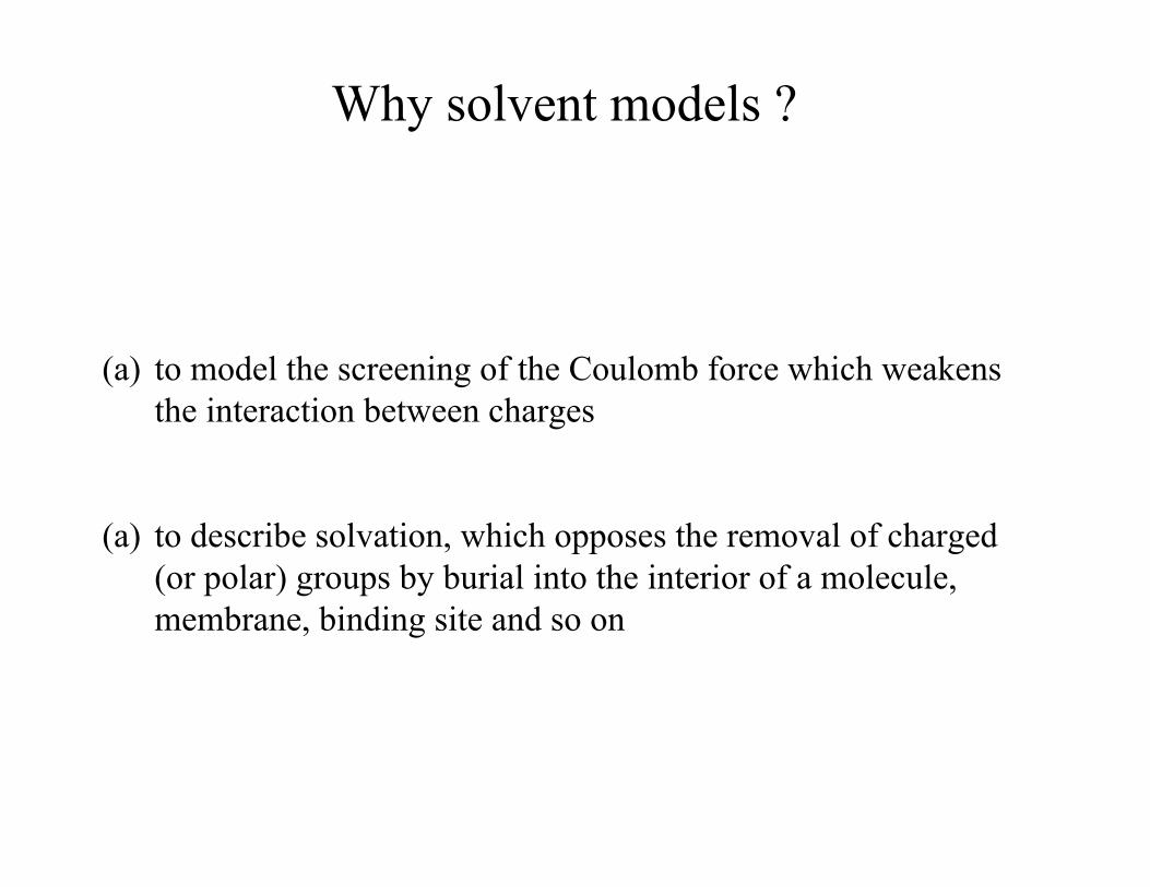
(a) to model the screening of the Coulomb force which weakens

the interaction between charges

(a) to describe solvation, which opposes the removal of charged

(or polar) groups by burial into the interior of a molecule,

membrane, binding site and so on

Why solvent models ?

Protein example goes here

(b) Coulomb force is long range

the potential varies with distance as 1/r

cf the attractive part of the van der Waals which varies as 1/r6

What is it about this Coulomb Force anyway?

(a) The Coulomb Force is strong

How strong:

If i was standing at arms length from Anthony and we each had

one percent more electrons than protons, then the repulsive force

would be enough to lift the weight of:

(i) Bob

(ii) Empire State Building

(iii) The Earth

+

- +

-

+

- +

-

npessolv GGG !+!=!

1G!

npG!solv

G!

2G!

21GGG

es!+!=!

vacuum

water

The Sheffield Model is concerned with the calculation of !Ges

0P =0!P

Continuum Solvation models capture average or “continuum”

behaviour of water. These theories favour information about

the role of water on say proteins or small molecules, rather

than information about structural features of water acting as a

solvent.

The Sheffield Model is a continuum model

Water is treated as a (linearly) polarizable dielectric.

The relatively high dielectric of water ("=80) means that it is

much more easily polarized than most solutes (proteins, small

molecules etc).

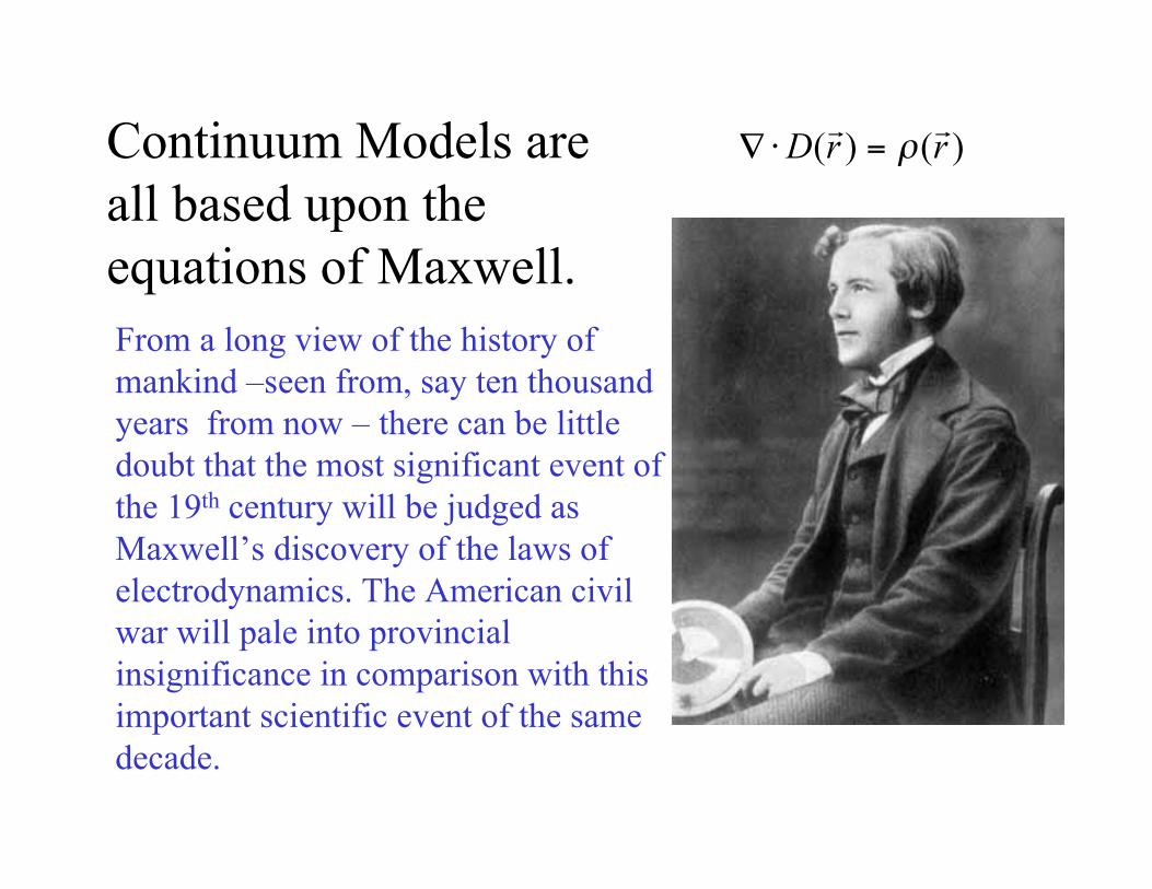
From a long view of the history of

mankind –seen from, say ten thousand

years from now – there can be little

doubt that the most significant event of

the 19th century will be judged as

Maxwell’s discovery of the laws of

electrodynamics. The American civil

war will pale into provincial

insignificance in comparison with this

important scientific event of the same

decade.

Continuum Models are

all based upon the

equations of Maxwell.

)()( rrDrr

!="#

Born (1920), Martin (1929), Bell (1931) (charge/dipole in a

spherical cavity)

Kirkwood(1934) (off-centred charges in spherical cavities)

Onsager (1935), Böttcher (1938) (polarizable dipole)

Debye H!ckel (1923) (theory of electrolytes)

Scholte (1949) (dipole in ellipsoidal cavity)

Tanford and Kirkwood (1957) (protein electrostatic models in the

days when proteins were spheres)

The Protagonists

and then a chance conversation led to ........

and then some things are never quite the same ever again ....

Classical electrostatics has also proved to be successful

quantitative tool yielding accurate descriptions of:

• electrical potentials,

•diffusion limited processes,

•pH-dependent properties of proteins,

•ionic strength-dependent phenomena,

• the solvation free energies of organic molecules.

Poisson Boltzmann Equation

(NB: not really atom based – dependency is on the spatial variation of the dielectric boundary)

So what is wrong with the Poisson Boltzmann Equation?

Well nothing much – it is the correct physical theory, but.....

•Implementations are difficult (requires multigrid FD solvers etc)

•Gradients are difficult to compute (especially high order

gradients)

•Computationally expensive relative to most classical modelling

approaches

•Difficult to combine with conventional modelling approaches

The alternative: Design bad atom-based solvation models

Take as starting point the fact that linear models can be written as

is the interaction of charged

atom(I) with the polarization it

produces in the dielectric

self

IE

is interactions of charged

atom(I) with the polarization

produced in the dielectric by

charged atom(J)

pair

IJE

+

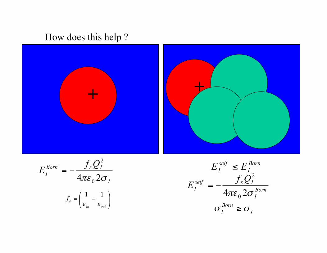
How does this help ?

!!"

#$$%

&'=

outin

f((

(

11

I

IBorn

I

QfE

!"#

#

240

2

$=

++

Born

I

Iself

I

QfE

!"#

#

240

2

$=

Born

I

self

I EE !

I

Born

I!! "

So far no Maxwell Equation has been hurt in the making of

this atom-based equation

But now comes GB theory

Invoke the “Coulomb Field” approximation

2

1

11

4

ˆ)(

I

II

r

Q

!

rrD =

which simplifies the potential produced as a result of dielectric polarization

! "#$$%

&''(

)**=

2

12

12112

ˆ)(1

)(

4

1)(

rd

in

pol rr

rrr

1

1 +,

,

-+

to:

2

12

12

2

1

111

0

2,

ˆˆ)(

4

1

4)(

rrd

Q

I

IIpol

IGB

rrrrr !"#= $ %

&&%'

!!"

#$$%

&'=(

)(

11)(

1

1r

r))

)in

NB:

)(4

11

8 4

0

2

rr !"= # $$% rd

QE Iself

I

Born

I

Iself

I

QfE

!"#

#

240

2

$=

! "= #$%

fr

dI

Born

I

)(1

4

114

rr

GB theory is the computation of #Born

augmented by a simple ansatz to account for the more complex pair

terms

20

2

4

IJ

cR

B

J

B

I

JIpair

IJ

Re

QQfE

BJ

BI

IJ

+

!=!

""

#

""$#

!!"

#$$%

&'=(

)(

11)(

1

1r

r))

)in

NB:

Stunningly Simple idea (number 1)

Construct a dielectric function based on atoms modelled

as Gaussian functions:

Computation of Born radii is complicated because of the arbitrary

shape of solvent regions displaced by atoms.

Stunningly Simple idea (number 2)

Also use a Gaussian “masking” function to

remove Coulombic singularities (from the expressions

for Born radii)

Subsequent Gaussian “mathematics” leads to analytic formulae

for Born radii, with smooth gradients to all orders. This is the

GGB model, which contains only a single adjustable parameter,

kappa, (associated with the range of the masking function).

What is so good about these Born radii anyhow?

20

2

4

IJ

cR

B

J

B

I

JIpair

IJ

Re

QQfE

BJ

BI

IJ

+

!=!

""

#

""$#

!+

"=IJ

IJJI

JIsolv

Sheff

bRa

QQfE

2

04 ##$%

%

or

Another Stunningly Simple idea – dispense with Born Radii:

Introducing the “Sheffield Solvation Model”.

!+

"=IJ

IJJI

JIsolv

Sheff

bRa

QQfE

2

04 ##$%

%

What is so good about these Born radii anyhow?

or

Another Stunningly Simple idea – dispense with Born Radii:

Introducing the “Sheffield Solvation Model”.

‘a’ acts to globally scale the atomic radii (i.e. models an average

local environment of a given type of atom characterised by a

radius of #)‘b’ controls the rate of switching of the pair term between long and

short range behaviour.

CH3

CH3

CH3

CH3

N

H

N

H

O

O

!"#$ "#% "& '()'*+", "-.*/ 0+)1 '()')2-3"% "'()'-.'45+-.3*657*/ 085

& 9:;*.5+5<=-+7457*95<0+40> 07)(1

PB(6gpa) : -18.61

Sheffield(a=1.553149,b=0.735694): -18.63

GGB(kappa=0.057768) -18.48

)( 1!" kcalmol

elec

solvG

Does the Sheffield Model actually work ?

Obtaining ‘a’ and ‘b’ ?

( )! "=Nmols

k

Shef

k

PB

k baEEbaF2),(),(

minimize a suitable “fitting” function eg

For example:

we considered 64 000 neutral and 387 charged molecules taken from the MDDR.

Structures built with Corina

radii and charges assigned based on the MMFF force field

F was minimized for ten different subsets of 10 000 randomly chosen molecules

Results

a = 1.553149 (0.0146)

b = 0.735694 (0.0108)

gratuitous picture of Jens

he did write Corina.

Comparison of solvation energies computed using the

Sheffield Solvation Model and the PB equation (for the MDDR set).

Percentage differences between solvation energies computed using

atom-based models and Poisson Boltzmann.

The solution entropy contains translational, rotational, and vibrational

contributions. Solvent effects were included in the vibrational term by

computing second derivatives of the molecular solvation energy. Normal mode

analysis yields harmonic force constants (from which is computed)

Calculation of Molecular Solution Entropies.

vib

solvS

Conformational energies!"#$ "#% "& '()'*+", "-.*/ 0+)1 ' ()')2-3"% "'()'-.'45+-.3*657*/ 085

& 9:;*.5+5<=-+7457*95<0+40> 07)(1

Oh dear

1

1

74.11)735694.0,553149.1(

38.10

!

!

!===

!=

kcalmol

kcalmol

baE

E

Sheff

PB

Optimizing a/b for this molecule

138.10)716365.0,892990.1( !!=== kcalmolbaESheff

An outlier:

What about proteins ?

Globally is fine for solvation energies as the below graph

(on a crude energy) scale shows.

However: a/b probably need a dependence on say solvent

accessibility/depth from surface for a more precise description.

of protein solvation.

What about Experiment?

• Data Set of 200 polar molecules

(Courtesy of Rob Rizzo, UCSF)

ZAP Using: GAST MMFF AM1BCC AM1BCC_U

RMS Expt (kcal): 3.62 2.68 1.55 1.31

With AM1BCC_U:

ZAP: 1.31

GB: 1.491

Sheffield: 1.495

Summary

even Barry can program it: for(i=0;i<N;i++) {

for(j=i,j<N;j++) Solvation+= -charges[j]*charges[i]/sqrt(A*dist+B*radii[j]*radii[i]);

}

Solvation*=0.50;

local model of solvation (not designed to predict individual pair

or self energies).

physics content is low but the model contains a minimal number of

parameters to deliver a relative high accuracy.

Sheffield Solvation Model is an exceptionally simple formula

could be considered a base line against which other more complex

models can be judged.

The End