the selection or seeding of college basketball or football teams for postseason competition

The Selection or Seeding of College Basketball or Football Teams for Postseason CompetitionAuthor(s): David A. HarvilleSource: Journal of the American Statistical Association, Vol. 98, No. 461 (Mar., 2003), pp. 17-27Published by: American Statistical AssociationStable URL: http://www.jstor.org/stable/30045190 .

Accessed: 14/06/2014 09:32

Your use of the JSTOR archive indicates your acceptance of the Terms & Conditions of Use, available at .http://www.jstor.org/page/info/about/policies/terms.jsp

.JSTOR is a not-for-profit service that helps scholars, researchers, and students discover, use, and build upon a wide range ofcontent in a trusted digital archive. We use information technology and tools to increase productivity and facilitate new formsof scholarship. For more information about JSTOR, please contact [email protected].

.

American Statistical Association is collaborating with JSTOR to digitize, preserve and extend access to Journalof the American Statistical Association.

http://www.jstor.org

This content downloaded from 185.2.32.121 on Sat, 14 Jun 2014 09:32:46 AMAll use subject to JSTOR Terms and Conditions

http://www.jstor.org/action/showPublisher?publisherCode=astata

http://www.jstor.org/stable/30045190?origin=JSTOR-pdf

http://www.jstor.org/page/info/about/policies/terms.jsp


The Selection or Seeding of College Basketball

or Football Teams for Postseason Competition David A. HARVILLE

Systems for ranking college basketball or football teams take many forms, ranging from polls of selected coaches or members of the media to so-called computer-ranking systems. Some of these are used in ways that have considerable impact on the teams. The committee

responsible for the selection and seeding of teams for the postseason National Collegiate Athletic Association (NCAA) Division I men's basketball tournament is influenced by various rankings, including ones based on the ratings percentage index (RPI). The Bowl

Championship Series (BCS) rankings of NCAA Division I-A football teams determine which two teams compete in a postseason national

championship game and determine eligibility for other prestigious postseason games. There are certain attributes that seem desirable in

any ranking system to be used in selecting or seeding teams for postseason competition or that may have some other tangible or intangible effect on the teams. These attributes include accuracy, appropriateness, impartiality, unobtrusiveness, nondisruptiveness, verifiability, and

comprehensibility. The polls, the RPI, and the BCS rankings are notably deficient in several of these attributes. A system having all of the attributes, except for unobtrusiveness, can be achieved by applying least squares to a statistical model in which the expected difference in score in each game is modeled as a difference in team effects plus or minus a home court/field advantage. The potential obtrusiveness of this approach can be circumvented by introducing modifications to reward winning per se and to eliminate any incentive for "running up the score" or for deliberately surrendering a lead so as to extend a game into overtime. The modified least squares system was applied to the 1999-2000 basketball and 1999-2001 football seasons. Its accuracy in predicting the outcomes of 73 postseason football games and 93 postseason basketball games was undiminished by the modifications and was comparable to that of the betting line.

KEY WORDS: Least squares; Paired comparisons; Prediction; Ranking; Rating.

1. INTRODUCTION AND BACKGROUND

Each spring, the National Collegiate Athletic Association

(NCAA) conducts a well-publicized and highly visible single- elimination tournament among a select 64 of the 300-plus men's basketball teams that compete in its Division I. The winner of this tournament is declared the national champion. With the exception of a few "independents," the Division I teams are organized into conferences, and their regular-season schedules include a large number of intraconference games and a typically smaller number of out-of-conference games. A team that belongs to an "elite" conference can guarantee itself a spot in the NCAA tournament by winning its conference championship. The remaining spots go to teams selected

by an NCAA committee.

Subsequent to rounding out the tournament field, the NCAA committee ranks the teams from first through last. It then

places each team in one of four "regional" brackets and seeds it from 1 through 16. In doing so, the committee is subject to various restrictions and attempts to adhere to certain principles. Perhaps the most important of these principles is that the brackets should be of similar strength and the seeds should be more or less consistent with the overall ranking.

In making its decisions, the committee has at its disposal a considerable amount of information. This includes not only basic statistics pertaining to each team's record, but also such

things as the results of the Associated Press (AP) and USA

Today/ESPN polls. It also includes rankings based on some-

thing called the ratings percentage index (RPI), which was devised for the specific purpose of assisting the committee.

A team's RPI is a weighted average of its winning percentage, the average winning percentage of its opponents, and the

average winning percentage of its opponents' opponents. At

present, these respective weights are 1/4, 1/2, and 1/4. This is the basic RPI. In practice, the NCAA uses a version that includes adjustments for factors that it has chosen to keep secret.

Since 1998, the NCAA (or, more accurately, an alliance comprising various of its "members") has engaged in an annual exercise in ranking and selection that generates perhaps even more public interest than that associated with its postseason Division I men's basketball tournament. Each Decem- ber/January after the regular season (and any conference

championship games), a select group of what are regarded as the best and/or most popular of the 100-plus football teams that compete in the NCAA's Division I-A are "paired up" in postseason games called "bowl games." In an attempt to improve on what had been a rather haphazard process for determining which teams participate and in which "bowls," the NCAA adopted a structure called the "Bowl Championship Series" (BCS). The BCS comprises a designated four of the most prominent bowl games, one of which is specified as the national championship game.

The decision as to which two teams play for the national championship and which teams qualify for participation in the other BCS bowl games involves a rather elaborate system for

ranking teams. In this system, a numerical "score" is established for each team by forming the sum of the following four components: (1) the average of its rank in the AP poll and its rank in the USA Today/ESPN poll; (2) an average of six of its eight possibly different ranks in eight "computer ranking"

David A. Harville is Research Staff Member Emeritus, Mathematical Sciences Department, IBM Thomas J. Watson Research Center, Yorktown Heights, NY 10598 (E-mail: [email protected]). The author is indebted to Thomas R. Boucher, who (while serving as a summer intern at the Wat- son Research Center) assembled, verified, and edited the college basketball data used in Section 4. The author is also indebted to the editor and several reviewers, whose comments and criticisms led to many improvements in the manuscript.

e 2003 American Statistical Association Journal of the American Statistical Association

March 2003, Vol. 98, No. 461, Applications and Case Studies DOI 10.1198/016214503388619058

17



18 Journal of the American Statistical Association, March 2003

systems, with the highest and lowest ranks excluded; (3) 1/25 times the rank of its strength of schedule, as measured by a weighted average of the winning percentage of its opponents and the winning percentage of its opponents' opponents, with weights of 2/3 and 1/3; and (4) its number of losses. The teams are ranked on the basis of their scores; the lower a team's score, the higher its ranking. Then an adjustment is made to each team's score for any wins over highly ranked teams, and the teams are reranked on the basis of the adjusted scores.

Some of the eight computer ranking systems are "propri- etary," and whatever descriptions may have been made public tend to be lacking in preciseness and detail to an extent that the rankings cannot be independently verified. The design of the strength-of-schedule (SOS) component appears to have been

inspired by the RPI (even with regard to the relative weights assigned to the records of a team's opponents and those of its

opponents' opponents). The descriptions of the four components are of those versions in effect for the 2001 BCS.

Much is at stake in the selection and seeding of basketball teams for the NCAA men's Division I tournament and in determining which Division I-A football teams compete in the four BCS bowl games. These decisions have large tangible or intangible effects on the athletes, the coaches, the fans, and the responsible administrators and can have a considerable direct or indirect impact on the financial support available to a university for its athletic and academic programs. Accord-

ingly, the decisions undergo much scrutiny and are frequently sources of controversy and criticism. Often it is the RPI (in the case of the selection and seeding of basketball teams) or the computer rankings (in the case of the BCS) that are at the heart of the controversy and criticism.

The ranking of teams has been the subject of considerable research. In much of the literature on this topic, the focus is on the accuracy of the rankings, as reflected in, for instance, their

ability to forecast the outcomes of future games. In determining whether a ranking procedure is appropriate for use in the selection or seeding of basketball teams for the NCAA tournament or in the BCS ranking exercise, accuracy is not the only consideration. Because of the potential impact of such use on the fortunes of the teams, various other attributes would seem to be desirable. These attributes are set forth in Section 2.

One well-established approach to the ranking of teams consists of applying a linear model to the difference in score from each game and of using least squares to arrive at the rankings (see, e.g., Leake 1976; Stefani 1977, 1980; Stern 1992, 1995; Harville and Smith 1994). The objective herein is to determine how this approach might be adapted for use in the seeding and selection of basketball teams for the NCAA tournament or in the BCS ranking procedure, and to make comparisons with current practices. In Section 3 the least squares procedure is described (along with the underlying statistical model), its shortcomings are identified, and various modifications are proposed for eliminating those shortcomings. Then in Sections 4 and 5 the modified least squares ranking procedure is applied to the results of the 1999-2000 college basketball season and the results of the 2001 college football season, and in Section 6 the predictive accuracy of the resultant rankings is evaluated. Finally, some concluding remarks are proffered in Section 7.

2. RANKING CRITERIA

What criteria should be adopted in designing or evaluating a ranking procedure when the rankings may play a part in decisions that affect various of the teams? Harville (2000, sec. 2), elaborating on, adding to, and updating an earlier list (Harville 1978, sec. 5), suggested that the procedure should have the following attributes:

1. Accuracy. That the rankings should accurately reflect the abilities of the teams seems obvious. What is less obvious is how to define and assess accuracy.

2. Appropriateness. The information used by the procedure should be restricted by considerations of appropriateness. The full or limited use of basic information about the outcome of each game played during the course of the current season seems appropriate. Examples of information that seems inap- propriate are information about games from previous seasons and information about conference affiliation.

3. Impartiality. A procedure can have this attribute only if it accounts for team-to-team differences in strength of schedule. One team may have a substantially more difficult schedule than another because the caliber of its opposition is higher or because a larger proportion of its games are played "away from home."

4. Unobtrusiveness. The use of the procedure should not affect the way in which the games are played. In particular, the procedure should provide a reward for "winning per se" and should not provide an incentive for "running up the score."

5. Nondisruptiveness. The procedure should not create incentives for otherwise undesirable changes in scheduling practices or conference affiliations (or independent status).

6. Verifiability. A complete description of the procedure should be readily available to all interested parties; this should be sufficiently detailed that the rankings can be independently verified.

7. Comprehensibility. The procedure should be sufficiently comprehensible so that it is understandable at an intuitive level

(and should be such that it is perceived to be sensible and

fair).

3. MODIFIED LEAST SQUARES RANKING PROCEDURE

In the (customary) least squares approach to ranking, each datum represents the difference in the (final) score between the two opposing teams in a game. Suppose that the differences in score are those from n games involving a total of t teams competing over the course of a single season. Let

rij repre-

sent the number of games in which the ith team is the home team and the jth team is its opponent, and for i and j such that r > 0, let yijk represent the difference in score between the ith and jth teams in the kth of those games. For any game played on a neutral court/field, arbitrarily (for notational purposes only) label one of the two opposing teams the "home team." Denote by xijk an indicator variable that equals 0 if the ijkth game is played on a neutral court/field and 1 otherwise (i.e., if the ith team is truly the home team).



Harville: Selection or Seeding of Teams 19

3.1 Underlying Model

One relatively simple and frequently adopted model for the differences in score is

Yijk = XijkAh + i - j +eijk ,

j: i= 1, ....

t; k= 1, . r...

, (1)

where the "team effects," p,/3 .... ,, (for the first through tth teams), and the "home-court/field advantage," A, are unknown parameters and where the eijk's are uncorrelated random residual effects with mean 0 and common unknown positive variance

o-2. Model (1) is a non-full rank model; a linear com-

bination cA + Et-= di4i of p,9 ..., Pt3 and A is estimable only if the coefficients satisfy the restriction >Jt di = 0. Typically, there are no other restrictions on estimability.

It is common to enhance model (1) by specifying that the

eijk's, and hence the yijd's,

are independently and normally distributed. This assumption is credible as well as convenient. Roughly speaking, a basketball or football game comprises a considerable number of more-or-less independent pairs of alternating possessions (opportunities to score), and the final difference in score is the sum of the differences in score from the various pairs of possessions. Thus the central limit theo- rem lends validity to the normality assumption.

Of course, strictly speaking, the distribution of the ijk' S cannot be normal (or even absolutely continuous); by their very nature, the yijk's are integer-valued, and hence their distribution is discrete. One way to account for the discreteness is to assume that corresponding to each Yiqk there is an underlying continuous variable, say Zijk, such that Yijk is determined by rounding zijk to the nearest integer, and to further assume that it is the zik's, rather than the Yijk's, that follow model (1), in which case

Zijk = Xijk i - j eijk, (2)

and, for every integer yijk

Pr(Yijk = Yk) = Pr(y-k - .5 Zijk< Y' .5), = i

r( ijk 5 ik _

ijk -!

)

j : i = l ....

,t; k = 1 ....

r1. (3)

For many (though not all) purposes, model (1) provides an adequate approximation to the model determined by equalities (2) and (3).

3.2 Basic Least Squares

If all pairwise differences among the team effects

/31 ..3. , , are estimable, then a statistical procedure for ranking college basketball or football teams can be obtained by fitting model (1) by least squares. Such a system was considered by Stefani (1980), Stern (1992, 1995), and Harville and Smith (1994), and an earlier version that ignored the home- court/field advantage was considered by Leake (1976) and Stefani (1977). It is subsequently assumed that all pairwise differences among the team effects are estimable and also that the home-court/field advantage is estimable.

Least squares estimates (of estimable functions) can be obtained from any solution to the normal equations. Using

"hats" to distinguish solutions/estimates from parameters and a "dot" to indicate summation over a subscript, the normal equations are

pA + qi = H (4) i

and

qiA + nipi - L niij -

= Di i 1 t (5)

j/i

where p = x... (n minus the number of games played on a neutral field), qi = xi.. - x.i. (number of home games played by the ith team minus the number of away games), H =

Lijk XijkYijk (total number of points scored by teams playing on their home courts/fields minus the total number scored against them), n, = rij + rji (number of games between the ith and jth teams), ni = ni. = n.i (number of games played by the ith team), and Di = yi.. + (-y.i.) (total number of points scored by the ith team minus the total number scored against it).

Least squares rankings are obtained by ordering the teams from first possibly to last in accordance with the /3,... 3, components of any solution to (4) and (5). Their solution is nonunique; however, it does not matter which solution is chosen. Every pairwise difference among 31 .... g, is invariant to this choice. Among the solutions to (4) and (5) is the solution obtained by imposing the constraint Ei nipi = 0, corresponding to the nonestimable restriction Ei nigi = 0.

It is instructive to reexpress the normal equations (4) and (5) as

=p-'1 kt [Yik-(/i- ( j)] (6) i, j k:xijk=l}

and

ni

Pi - nT1 (dis - uis, + Js),

i= 1 ... t, (7)

s=l

where for the sth of the ith team's ni games, dis denotes the

difference in score between the ith team and its sth opponent, ui, equals o1 or 0 depending on whether the game is a home or away game for the ith team or is played on a neutral court/field, and ji, identifies the opposing team. These expressions are amenable to intuitive interpretation. The estimate of the home court/field advantage is obtainable by adjusting and then averaging the p differences in score between the home and visiting teams. The adjustments are for the relative strengths of the opposing teams, and games played on a neutral court/field are not included in the averaging (though they do affect the adjustments). The rating (/3) for the ith team is obtained by adjusting and then averaging the ni differences in score between the ith team and its opponents; the adjustments are for any home-court/field advantage and for the opponents' strength (as reflected by their ratings).

A solution to the normal equations could be computed by any of a number of direct methods for solving linear systems of equations using readily available software. Alternatively, one could attempt to use (6) and (7) to compute a solution




iteratively via the so-called "method of successive approxi- mations." However a solution might be computed, its validity could be partly or completely verified by any interested party through a simple (though potentially tedious) exercise in which the solution is substituted into some or all of (4) and (5) or (6) and (7).

3.3 Key Modification: Limited Use of Margin of Victory

The basic least squares ranking procedure is potentially obtrusive. If it were used in the selection and seeding of basketball teams for the NCAA tournament or in the BCS ranking procedure, then it would have an impact on the way in which the "regular season" games (on which the rankings are based) are played. The procedure places no emphasis on winning per se, and allows a team to enhance its ranking by running up the score.

Incentives for running up the score beyond a specified (positive) number of points, say C, can be avoided by using a

ranking procedure in which the effect on the rankings of a

margin of victory of more than C points is exactly the same as one of C points. In the "extreme" case where C = 1, this

approach leads to rankings based entirely on win-loss-tie information, which provide no incentive whatsoever for running up the score. Note that such an incentive cannot be avoided simply by "downweighting" the effects of margins of victory that exceed C points. In fact, it is conceivable that teams might "react" to the downweighting by trying for even larger margins of victory.

A very straightforward way of modifying the basic least squares ranking procedure (or other ranking procedure) so as to eliminate the influence of margins of victory exceeding C

points is to replace every such margin by C and to proceed as before; that is, apply the procedure to the truncated (at sC) differences in score. When model (1) is applied to the truncated differences rather than to the untruncated differences, the

assumptions of additivity (of the home court/field advantage and of the team effects) and of homogeneous variance can be

very unrealistic, especially for a small value of C. This suggests that application of the basic least squares procedure to the truncated differences may have undesirable consequences that go beyond any loss in overall accuracy. One such con-

sequence is that under certain circumstances, the inclusion of the truncated difference from an additional game can have a negative impact on the ranking of the victorious team even if the margin of victory is C or more points (e.g., Harville 2000, sec. 3.2).

A possibly more appealing modification of the basic least- squares ranking procedure can be obtained by adopting a tech- nique proposed by Harville (1977, sec. 3.2; 1978, sec. 5). This modification involves replacing each difference yijk with the quantity yijk (C) defined as

EzijkZij >C- 2 if Yi, > C

Yijk (C) Yijk if - C < Yijk < C

E zijk Zijk < C+ if Yjk < -C.

Here the conditional expected values E(ijk I Zijk > C - 1/2) and E(ijk Izijk < -C + 1/2) are those obtained by assuming that Zijk follows model (2) and that eijk is normally distributed; they are obtainable from the formula

ijk -t- oh[(C - 1/2 FLijk1)/0], (8)

where taijk = xijk + Pi - Pj and h(.) is the so-called haz-

ard (rate) function of the standard normal distribution (e.g., Johnson, Kotz, and Balakrishnan 1994, p. 156). The requisite values of the hazard function can be obtained from existent tables. Alternatively, any of a number of standard software packages can be used to construct a table of such values or to compute them on demand.

In the proposed modification of the basic least squares ranking procedure, Yijk is replaced by Yijk (C). Whenever Yijk > C or Yijk < -C, this quantity is functionally dependent on a2 and also (through b/ijk) on A, Pi, and 3j. In implementing the proposed modification of the basic least squares system, the value of Yijk (C) is taken to be that obtained by assigning

a.2 an esti-

mated value, say ^-2, and by setting A, /i, and 3j equal to A,

/3i, and 3j. Then, subsequent to modification by replacing the

Yijk ' by the yijk(C)'s, the right sides of (4) and (5) depend on A, P/,,... ,/3, and hence the (formerly linear) system comprising these equations must be solved iteratively.

It can be shown that if 0"2 is taken to be what is the maximum likelihood estimator of U2 when the truncated (at +C) differences in score are regarded as the data (or in the hypo- thetical case where o.2 is known, to be 0-2 itself), then (when the truncated differences are regarded as the data) the solution A, 31,,..., /3t to the modified normal equations is a maximum likelihood "estimator." In practice, it may be preferable to take

2 Se/(ln - t), (9)

where Se is the residual sum of squares obtained from a least squares fit of model (1) to the (untruncated) yijk's. It seems unnecessary to impose restrictions on the information to be used in estimating a2, and unlike the maximum likelihood estimator of o2, estimator (9) (the ordinary unbiased estimator) accounts for the t degrees of freedom lost in fitting A, /f 1 ..., zt.

The hazard function h(e) is plotted in Figure 1. This figure can be used in conjunction with expression (8) to develop a sense for how jijk(C) is affected by /ijk, o-, and C. Consider, for instance, the case where A ijk is much larger than C or much smaller than -C. In this case, yijk(C) is close to Lijk if Yijk is "as anticipated"; when A.ijk >> C, it is anticipated that

Yijk> C and when Iijk << -C, it is anticipated that yijk < -C. This implies that under the proposed modification of the least

squares ranking procedure, the rankings are not much affected by the outcome of a game in which a team defeats a much lower-ranked opponent by C or more points.

The proposed modification is such that the potential incentive for a team to run up the score (beyond a difference in score of C points) is eliminated. However, strictly speaking, it is only in the special case where C = 1 that the modified procedure provides a reward for winning per se. Choosing C = 1

may degrade the accuracy of the procedure to an undesirable




5

4

3

h(s)

2

1

0

-4 -2 0 2 4 s

Figure 1. Hazard Function h(-) of the Standard Normal Distribution.

extent. This suggests (Harville 1977, 1978) a hybrid version of the modified system in which (in carrying out the least squares analysis) a weighted average,

W~ijk(l) (1 - w)Yijk (C) (10)

(where 0 < w < 1), is substituted for Yijk,. The weight, w, and the "threshold", C, can be chosen (on the basis of input from the relevant parties) to strike a suitable balance among accuracy, providing a reward for winning per se, and avoiding any potential incentive for running up the score.

3.4 Other Modifications

3.4.1 Shrinkage. There is a potential pitfall to be avoided in any implementation of the modified least squares ranking procedure. A solution to the (unmodified) normal equations (4) and (5) always exists. However, when these equations are modified by replacing each Yijk with weighted average (10), the existence of a solution is no longer a certainty. This problem is encountered when some team, say the ith team, has won all of its games (or, alternatively, lost all of its games) by C or more points. Under such circumstances, the ith of (5) does not (subsequent to its modification) have a finite solution. The occurrence of the problem could be rendered highly improb- able by assigning C a "reasonably large" value; however, it may be preferable to introduce a change so as to eliminate the problem altogether.

Partition the first t positive integers (corresponding to the t teams) into mutually exclusive and exhaustive subsets, say Sl, ..., Sc, corresponding to divisions (one of which is Divi- sion I or I-A). In assimilating the proposed change, it can be helpful to think of ,,

.f... ,3, not as parameters, but rather

as uncorrelated random variables such that for i E Sk (and for some scalars ALk and r2), E(f i) = -k and var(i) = =7 (k = 1, ... ,c)--,1 . f. , t could be regarded as "random effects." Further, for k = 1 ... , c- 1, take lk to be an estimate (obtained from the past and/or present data) of the "mean

difference" between the kth and cth divisions; think of 1k as an estimate of

uk -

c. In addition, take /c = 0, thereby estab-

lishing the cth division as the "base division." Now, instead of basing the rankings on the ,

.... , ,t

components of a solution to (4) and (5), consider basing them on the 3, ... 3t components of the solution (for 81.

... 0q ,i1

.. P*t, and A) to (4) and the equations

niIlk + qi + (ni + y)i - L niij - =Di, jAi

iESk; k=l1..., c, (11)

and

i = -lk

+ i, i E Sk; k = 1 ....

, c. (12)

Here y is a positive scalar whose presence introduces some "shrinkage" into the least squares ranking procedure. In practice, the right sides of (4) and (11) are to be modified by replacing each yijk with weighted average (10). Even after that modification, a solution to (4), (11), and (12) always exists. Note that "solving" (11) for 8~, . . , 8, and substituting the resultant expressions into (12) leads to the expressions

ni

S-Lk (ni + y)-)1 Z (dis - Lk -- uiA + ) s=1

ie Sk;k 1 ...., c.

These expressions can be regarded as the counterparts of expressions (7).

If (when regarded as random) the team effects 3 1.... fit were truly uncorrelated, then (assuming that they had a

common variance, say 72), it would be appealing (from the perspective of either best linear unbiased prediction or empirical Bayes estimation) to take y to be an estimate of '2/r2 (Harville 1977, 1978). However, taking y to be that large has undesirable consequences; it may result in teams with weak schedules being considerably overrated and those with strong schedules being considerably underrated. The effects of this are exacerbated by the "nonrandomness" of the schedule; conditional on the schedule (i.e, on the rij's), the team effects are positively correlated.

Any undesirable effects of basing the rankings on (4), (11), and (12) can be minimized by settling on a relatively small value of y (and the resultant small amount of "shrinkage"). A small value is enough to ensure that a solution to (4), (11), and (12) continues to exist subsequent to modification (and may have some beneficial effect on the overall accuracy of the rankings). It is worth noting that an estimate of the mean difference between the kth and cth divisions (k = 1,.... , c- 1) can be obtained from the rankings data by augmenting (4), (11), and (12) with the equations

ni j )

j

k +

'iS

) nij )

8i- ij)Pi =sk jVSk / iESk iESk jVSk iVSk jESk

(ij.-ji.), k 1 .. c - 1 (13) iESk jVSk

(Harville 2002, sec. 4.3).




3.4.2 Overtime Periods. If at what would normally be the end of a college basketball or football game the score is tied, the game is extended. The extension consists of a suc- cession of overtime "periods"; in college basketball, 5-minute

periods, and in college football, a pair of alternating possessions. Play continues until an overtime period is completed with one team having outscored the other. The basic or (if C > 1) modified least squares ranking procedure has the undesirable feature that a team about to win a game by a small

margin could possibly enhance its ranking by deliberately sur-

rendering a tieing score and by then winning (in overtime

play) by a bigger margin. A ranking procedure should not provide any incentive for a team to extend a game from "regulation play" to overtime or from one overtime period to another, except to improve its chances of winning the game. This suggests that any reward for winning per se should be no larger for a team that wins in an overtime period than for one that wins in regulation play or an earlier overtime period. It further suggests that the margin of a victory or defeat in overtime should not affect a team's ranking.

Accordingly, some adjustments in the modified least squares ranking procedure are proposed. For this purpose, let yijk represent the difference in score in the ijkth game at the end of

regulation play. Take the model for the y(0) to be that defined

by (2) and by the equality obtained from (3) by replacing Yijk by y(0) [as opposed to taking the model for the final differences in score to be that defined by (2) and (3)]. Further, denote by

fii the number of overtime periods required to complete the

ijkth game. The proposed adjustments in the modified least-

squares ranking procedure are those that result from making certain alterations to Yijk(1) and yijk(C) in forming weighted average (10). These alterations are contingent on eijk > 0 (i.e., are confined to overtime games). When eijk > 0, Yijk(C) is set to 0. As for the alteration of yijk (1), one relatively simple pos- sibility is to replace yijk(1) (when eijk > 0) with

E(zijk I zijk > 0) or E(zijk I Zijk < 0), (14)

depending on whether Yijk > 0 or Yijk <0 (i.e., on which team

ultimately wins). An alternative to quantity (14) as a replacement for Yijk (1)

is obtained by modeling the differences in scores from the successive overtime periods as an infinite sequence of independently and identically distributed random variables whose common distribution is that of a variate obtained by round-

ing from a normally distributed variate, say z k, with E(zk,) E(Zijk)/a and var(zk ) = var(zijk)/a (where a > 1). The moti- vation for this comes from regarding each overtime period as a fraction 1/a of a game of standard length (which is more realistic for college basketball than for college football). The alternative to using quantity (14) as the replacement for Yijk (1) is to use the conditional expected value of Zijk given that the ith team wins in no more than eijk overtime periods, or (depending on the final outcome of the game) the conditional expected value of Zijk given that the jth team wins in no more than fijk

overtime periods, which can be expressed as

E(zijk I +Zjk >1

Pr(mzjk >2) X

(15)

where 0 = Pr(- i<k z<k ).

4. 1999-2000 COLLEGE BASKETBALL

The modified least squares ranking procedure was applied to the outcomes of NCAA men's college basketball games for the 1999-2000 "regular" season. For the purpose of judging the effects of the proposed modifications, the basic least

squares ranking procedure was also applied. The end of the

regular season came on March 12th, and (as usual) coincided with the meeting of the NCAA committee to complete and seed the tournament field. The games whose outcomes were used in the least squares rankings were all those from the regular season in which one or both of the opposing teams were from Division I; outcomes of games in which neither team was from Division I were not available for the study. There were 4,815 such games, involving a total of 319 Division I teams and 186 non-Division I teams.

In implementing the modified least squares procedure, the

weight w was taken to be .5, and the cutoff point C was 19-values within a range that would seem widely acceptable. No "shrinkage" was used; the number of games played by a college basketball team is sufficiently large (around 30) that (for reasonable values of y) shrinkage is unlikely to have much effect on the rankings. The modification for overtime periods was invoked, with the form of this modification taken to be that in which the replacement for Yijk (1) is that given by (15). Of the 4,815 games, 230 (4.8%) were decided in overtime: 194 in one overtime, 28 in two overtimes, 6 in three overtimes, and 2 in four overtimes. Based on an informal com-

parison of various characteristics of the empirical distribution of the number of overtimes with the corresponding characteristics of a geometric distribution, a was taken to be 18. If a were 8 (its "theoretical" value, based on an overtime period being 1/8 as long as regulation play), then the expected number of multiple-overtime games (out of 230) would be approx- imately 25, which is considerably smaller than the observed number (36). A possible explanation is that teams tend to

adopt a more cautious approach in overtime play than in regulation play.

The basic least squares rankings were obtained from a least

squares analysis in which model (1) was fit to the final differences in score (without regard to whether the games were decided in overtime). The estimate of o obtained [on the basis of (9)] from that analysis was 10.4. A similar estimate was obtained from a separate least squares analysis in which the data comprised the differences in score at the end of regulation play. This estimate of or was used subsequently in obtaining the modified least squares rankings. The basic least squares estimate of the home-court advantage was 4.19 (with an estimated standard error of .17), and the modified least squares estimate of the home-court advantage was 4.36.




These estimates are slightly lower than the estimate of 4.68 obtained by Harville and Smith (1994) from a least squares analysis of 1,678 games from the 1991-1992 season.

The "ratings" obtained by modified and basic least squares are presented in Table 1. Each team's rating is the estimate of the difference between its team effect and the average Divi- sion I team effect. The estimated standard errors of the basic least squares ratings were readily obtainable and were found to be quite uniform, with a range (among Division I teams) of 1.90 (for Connecticut) to 2.34 (for Alabama State). The most poorly estimated pairwise difference in team effects was that between Eastern Washington and Alabama State, with an esti-

mated standard error of 3.28. In addition to each team's ratings, Table I gives the average of the modified ratings of each team's opponents, each team's won-lost record, each team's rank (if among the top 25) in the AP and USA Today/ESPN polls, and each team's RPI [both the "total" and an SOS component consisting of 2/3 of the average of the winning percentages of the team's opponents plus 1/3 of the average of the winning percentages of its opponents' opponents]. Further, for teams included in the 64-team NCAA Division I men's basketball tournament, Table 1 indicates the region to which it was assigned, how it was seeded, and the number of tournament games that it won.

Table 1. Rankings/Ratings of NCAA Division I Men's Basketball Teams (1999-2000 season)

Least squares Polls (rank) RPI

Rank Team Modified Basic SOS W-L AP USA Total SOS Tournament

1 Cincinnati 25.2 24.6 8.2 28-3 7 6 .6657 .5865 2S/1 2 Stanford 25.1 25.9 5.8 26-3 3 3 .6246 .5351 1S/1 3 Michigan State 22.7 23.3 8.4 26-7 2 2 .6183 .5618 1M/6 4 Duke 22.4 25.1 7.1 27-4 1 1 .6413 .5648 1E/2 5 Temple 20.7 21.1 7.2 26-5 5 5 .6309 .5616 2E/1 6 Florida 20.1 21.8 5.8 24-7 13 11 .6105 .5560 5E/5 7 Tulsa 19.3 19.2 1.0 29-4 18 19 .5997 .5067 7S/3 8 Arizona 19.2 18.0 9.0 26-6 4 4 .6378 .5796 1W/1 9 Oklahoma State 19.0 19.6 4.1 24-6 14 15 .6087 .5472 3E/3

10 Texas 19.0 19.7 9.0 23-8 15 18 .6282 .5903 5W/1 11 Iowa State 18.8 17.0 4.4 29-4 6 7 .6322 .5540 2M/3 12 Oklahoma 18.1 17.9 6.2 26-6 12 13 .6220 .5585 3W/1 13 Indiana 17.8 18.9 9.4 20-8 22 17 .6048 .5683 6E/0 14 LSU 17.5 18.1 4.5 26-5 10 9 .6194 .5463 4W/2 15 Syracuse 17.5 16.3 4.9 24-5 16 14 .6173 .5473 4M/2 16 Illinois 17.4 18.8 8.5 21-9 21 23 .5971 .5628 4E/1 17 Ohio State 17.3 16.4 6.2 22-6 8 8 .5966 .5335 3S/1 18 Connecticut 16.5 16.1 7.1 24-9 20 21 .6162 .5791 5S/1 19 Tennessee 16.5 17.7 5.6 24-6 11 10 .6199 .5622 4S/2 20 Kentucky 16.3 16.9 10.5 22-9 19 20 .6378 .5796 5M/1 21 Kansas 16.3 17.0 8.1 23-9 .6117 .5790 8E/1 22 Maryland 15.6 17.8 8.3 24-9 17 16 .6172 .5806 3M/1 23 Purdue 15.6 15.4 7.3 21-9 25 24 .5830 .5474 6W/3 24 St. John's 15.4 13.5 6.5 24-7 9 12 .6354 .5891 2W/1 25 Wisconsin 15.1 14.9 10.9 18-13 .5828 .5835 8W/4 26 Gonzaga 14.9 16.7 3.4 24-8 .5823 .5264 10W/2 27 Louisville 14.2 14.7 7.5 19-11 .5845 .5724 7W/0 28 North Carolina 14.0 15.0 8.9 18-13 .5769 .5757 8S/4 29 Oregon 13.7 14.1 6.4 22-7 .5945 .5427 7E/0 30 DePaul 13.6 14.0 6.1 20-11 .5833 .5627 9E/0 31 UCLA 13.3 13.6 8.9 19-11 .5911 .5770 6M/2 32 Kent State 12.6 11.6 2.6 21-7 .5811 .5312 33 Auburn 12.4 12.7 5.5 23-9 24 22 .5987 .5617 7M/1 34 Butler 12.2 12.4 -.1 23-7 .5645 .4971 12E/0 35 Pepperdine 12.2 12.9 1.9 24-8 .5681 .5074 11E/1 36 UNLV 12.1 8.8 1.5 23-7 .5690 .5031 10M/0 37 Southern California 11.8 13.5 7.8 16-14 .5474 .5521 38 Vanderbilt 11.7 11.7 6.4 19-10 .5774 .5515 39 UNC Charlotte 11.6 11.6 8.5 17-15 .5630 .5736 40 Missouri 11.4 11.6 7.7 18-12 .5789 .5719 9S/0 41 Utah State 10.9 9.1 -.5 28-5 .5924 .5140 12S/0 42 Dayton 10.8 9.8 3.6 22-8 .5736 .5204 11W/0 43 Utah 10.8 11.3 2.8 22-8 .5690 .5206 8M/1 44 Ball State 10.7 8.5 3.9 22-8 .5731 .5227 11M/0 45 Miami (FL) 10.5 9.9 4.1 21-10 23 25 .5805 .5482 6S/2 49 Seton Hall 10.1 8.7 3.9 20-9 .5693 .5291 10E/2 51 St. Bonaventure 10.1 9.7 5.4 21-9 .5773 .5364 12M/0 53 St. Louis 9.6 8.3 8.3 19-13 .5827 .5791 9M/0 59 Fresno State 9.1 8.3 3.1 24-9 .5945 .5503 9W/0 61 Creighton 9.0 8.4 1.4 23-9 .5608 .5081 10M/0 65 SW Missouri State 8.8 7.6 4.3 22-10 .5824 .5474

NOTE: The results for the RPI are those compiled (for the basic version) by Jerry Palm and made available by him at http://www.collegerpi.com. The first part of a team's entry under the heading tournament indicates whether it was selected for the 64-team NCAA Division I men's basketball tournament and (if so) its assigned region (East, Midwest, South, or West) and its seed (1-16) within the regional field; the second part gives the number of tournament games that it won.




Judging from the modified least squares rankings, Kent State deserved to have been included in the tournament field; St. John's and Miami (both of whom are members of the Big East Conference) received seeds appreciably "higher" than warranted; and Tulsa, Florida, Gonzaga, and Butler received seeds appreciably "lower" than warranted. There were some substantial differences between the rankings produced by modified least squares and those produced by the RPI. In particular, Fresno State, St. John's, and Kentucky were ranked much lower and Florida, Michigan State, and Oklahoma State

appreciably higher by modified least squares than by the RPI.

5. 2001 COLLEGE FOOTBALL

The modified and basic least squares ranking procedures were applied to the outcomes of NCAA football games from the 2001 "regular" season (which ended on December 8). The

rankings were based on the outcomes of all games in which both teams were among those in the "top" three divisions

(I-A, I-AA, and II). There were 2,018 such games (including 57 that pitted a Division I-A team against a Division I-AA team and 68 that pitted a Division I-AA team against a Division II team), and altogether these three divisions com-

prised 385 teams, 117 of which were Division I-A. As in the basketball application, the basic least squares rankings were obtained by fitting model (1) to the final differences in score

(without regard to whether the games were decided in over-

time). The cutoff point C in the modified least squares procedure

was taken to be 21 for games in which either or both teams were Division I-A and was taken to be infinite for games in which neither team was Division I-A (under the presumption that the rankings would not affect teams that were not Division I-A and would not provide any incentive for them to run up the score). The choice C = 21 is consistent with what (in the

past) has been acceptable to those who administer the BCS. Several values of w were tried, starting with .5 and ranging upward to 1.

Due to the relatively modest number of regular-season games played per team (typically 11 or 12), shrinkage was used in implementing the modified least squares ranking procedure. Proceeding as described in Section 3.4.1, the 385 teams were partitioned into c = 3 subsets: S,, comprising the Division I-AA teams; S2, comprising the Division II teams; and S3 (the base subset) comprising the Division I-A teams. And, based on the empirical results of Harville (2002), y was taken to be .5. For games decided in overtime, the weighted average (10) was altered in the way described in Section 3.4.2, and the replacement for yjk (1) in this alteration was taken to be that given by expression (14). Of the 2,018 regular-season games, 59 (2.9%) were decided in overtime: 39 in 1 overtime, 14 in 2 overtimes, 4 in 3 overtimes, I in 4 overtimes, and 1I in 7 overtimes.

The modified least squares rankings were based on the

/,, ... f, components of the solution to the linear system

comprising (11) and (12) along with equations obtained from (4) and (13) by introducing alterations for the incorporation of information from previous seasons about A and about the divisional differences

/, - /l3 (I-AA vs. I-A) and /L2

--,3 (II vs. I-A). Based on estimates obtained for previous seasons

by Harville (2000, 2002), o- was assigned (in carrying out the modified least squares analysis) a value of 13.5. In comparison, the estimate obtained from the basic least squares analysis of the differences in score from the 2001 season was 13.9. The solution obtained for the "estimates" of A, A~ - /13, and

-L2 - /3 were A = 4.1, 1, = -28.4, and ,2 = -40.4 when w = .5 and A = 4.2, 1, = -28.4, and /2 = -38.4 when w = 1. The estimate of A obtained from the basic least squares analysis (without any use of information from previous seasons) was 3.4 (with an estimated standard error of .3). This is a bit lower than the estimates (3.8 + .3 and 4.2 a .3) reported by Harville (2000, 2002) for the 1999 and 2000 seasons.

Table 2 gives basic and modified least squares "ratings" for each of a number of teams. There are two sets of modified

ratings. The first set comprises those obtained when w = 1/2 (and are those on which the ranking is based); the second set, those obtained when w = 1. The estimated standard errors of the basic least squares ratings of the Division I-A teams

ranged from a low of 4.17 (for BYU) to a high of 4.67 (for Arizona), and the largest estimated standard error of the pairwise differences in ratings was 6.79 (for Arizona vs. Wake

Forest). The entry for each team in the SOS column of Table 2 is the average rating of the team's opponents plus or minus an adjustment for the home-field advantage (where both are for modified least squares and for w = 1/2). Table 2 also

gives each team's won-lost record, its rank in the two polls (if among the top 25), and its "rating" (both overall and on SOS) in the BCS procedure. The BCS ratings (in which lower is

better) are given only for those 15 teams with the best overall

ratings. The last column of Table 2 gives the pairings for the

postseason bowl games (of which there were 25). The modified least squares rankings were considerably

affected by the choice of w. Those obtained by taking w = 1 are more in conformance with the polls than those obtained by taking w = .5 (which bear some resemblance to the basic least

squares rankings) and those obtained from the BCS "ratings." Taking w = 1 (instead of w = .5) elevates Oregon from ninth to second, ahead of Nebraka, which was second in the BCS

rankings and (as a consequence) qualified to play the highest- ranked team (Miami) in the national championship game.

6. PREDICTIVE ACCURACY: EMPIRICAL RESULTS

The ability of the modified least squares rankings to forecast the outcomes of future games provides a highly relevant mea- sure of their accuracy. Accordingly, the modified least squares rankings/ratings of Division I college basketball teams for the 1999-2000 season were used to forecast the outcomes of 95 postseason tournament games. The 64-team NCAA tournament comprised 6 rounds and a total of 63 games. In addition, there was a National Invitational Tournament (NIT), with a 32-team field chosen from those teams not included in the NCAA tournament. The NIT comprised 5 rounds and a total of 32 games. Except for the first three rounds of the NIT (in which the games were played on the home courts of one or the other of the opposing teams), the tournament games were (with very occasional exceptions) played on neutral courts.

It is of interest to assess the accuracy of the modified least squares rankings/ratings not only in absolute terms, but




Table 2. Rankings/Ratings of NCAA Division I-A Football Teams (2001 regular season)

Least squares Polls (rank) BCS

Rank Team Modified 1/2 Modified 1 Basic SOS W-L AP USA Total SOS Bowl

1 Miami (FL) 33.8 30.7 35.8 1.9 - .4 11-0 1 1 2.62 .72 W-1 2 Florida 25.0 20.4 30.8 3.6-1.1 9-2 5 5 13.09 .76 W-2 3 Texas 24.9 20.1 28.9 2.5 + 0 10-2 9 9 17.79 1.32 W-17 4 Nebraska 21.1 23.2 25.0 3.4-1.4 11-1 4 4 7.23 .56 L-1 5 Oklahoma 19.2 17.4 22.1 2.7-1.0 10-2 10 10 21.54 1.44 W-8 6 Colorado 18.8 22.4 18.7 7.8 - .7 10-2 3 3 7.28 .08 L-4 7 Tennessee 18.4 21.8 16.7 6.8 - .3 10-2 8 8 14.69 .12 W-5 8 Washington State 17.1 20.8 12.7 .4 - .4 9-2 13 13 26.91 1.68 W-12 9 Oregon 16.4 24.0 15.9 4.2 - .4 10-1 2 2 8.67 1.24 W-4

10 Illinois 15.5 20.6 13.9 2.2 - .4 10-1 7 7 19.31 1.48 L-3 11 Stanford 15.1 21.0 12.6 4.9 - .4 9-2 11 11 20.41 .88 L-21 12 Virginia Tech 14.2 8.2 18.4 -.6 - .4 8-3 15 16 L-6 13 UCLA 13.8 14.1 14.3 6.1 + .4 7-4 14 Michigan 13.7 12.9 15.6 4.3 - .4 8-3 17 15 L-5 15 Kansas State 13.5 9.2 21.0 6.8 - .4 6-5 L-14 16 Fresno State 13.4 16.7 14.1 -2.2 + .3 11-2 20 21 L-11 17 Maryland 13.4 20.4 13.7 -2.7-1.1 10-1 6 6 21.29 3.12 L-2 18 Georgia 12.7 14.9 10.0 .7 - .4 8-3 16 19 L-18 19 Florida State 12.4 11.9 15.2 6.2 - .4 7-4 24 24 W-6 20 BYU 12.0 16.2 10.6 -5.0 + .3 12-1 19 17 L-10 21 LSU 11.9 15.5 11.4 4.5-1.0 9-3 12 12 27.73 .40 W-3 22 Syracuse 11.9 14.7 10.8 5.0 - .3 9-3 18 18 W-14 23 South Carolina 11.7 14.6 9.3 3.3-1.1 8-3 14 14 37.77 1.60 W-7 24 Marshall 11.3 13.5 4.6 -5.7 + 0 10-2 25 W-24 25 Texas Tech 11.0 8.1 16.6 4.0 - .4 7-4 L-15 26 Boston College 10.7 5.8 10.3 .6 - .4 7-4 W-18 27 Louisville 10.2 11.2 8.1 -4.9 + 0 10-2 23 22 W-10 28 Southern California 9.2 7.0 13.1 4.6 - .4 6-5 L-22 29 Washington 8.5 16.9 4.9 6.4 - .4 8-3 21 20 38.17 0.84 L-17 30 Ohio State 8.5 7.9 10.3 2.8 - .4 7-4 22 23 L-7 31 North Carolina 8.4 9.1 10.4 4.5 + 0 7-5 W-9 32 Utah 8.3 5.9 9.7 -1.0 + .4 7-4 W-22 33 Texas A&M 8.2 10.8 9.1 5.8 - .4 7-4 W-19 34 Iowa 8.0 3.2 15.9 2.5 - .4 6-5 W-15 35 Alabama 7.8 6.7 9.0 3.3-1.1 6-5 W-20 36 North Carolina State 7.2 7.0 7.3 -.4- .4 7-4 L-23 37 Georgia Tech 6.9 6.2 9.2 -.2- .3 7-5 W-21 38 Arkansas 6.8 11.0 4.1 3.6-1.1 7-4 L-8 39 Iowa State 6.4 7.8 9.1 2.5 - .4 7-4 L-20 40 Bowling Green 5.9 5.8 4.9 -4.2 + .4 8-3 41 Toledo 5.4 7.1 -.3 -7.9 - .4 9-2 25 W-16 42 Hawaii 5.3 7.2 5.0 -5.3- 2.0 9-3 43 Auburn 5.3 11.7 2.3 5.6 - .4 7-4 L-9 44 Boise State 4.8 8.6 3.6 -5.0 - .3 8-4 49 E. Carolina 3.7 -.1 4.2 -2.0 + .4 6-5 L-24 50 Louisiana Tech 3.6 6.1 .2 -3.9+1.5 7-4 L-13 51 Clemson 3.6 5.1 2.2 1.0 - .4 6-5 W-13 52 Michigan State 3.6 1.9 8.6 1.3 - .4 6-5 W-11 53 Pittsburgh 3.3 .8 4.8 1.3 - .4 6-5 W-23 57 Purdue 1.8 3.7 3.6 3.7 - .4 6-5 L-12 58 Colorado State 1.7 3.3 1.2 1.8 + 0 6-5 W-25 69 TCU -1.8 -2.8 -1.0 -4.7+1.1 6-5 L-19 77 Cincinnati -3.2 -2.4 -4.3 -8.7 - .4 7-4 L-16 89 North Texas -8.7 -9.0 -7.6 -8.3 + .4 5-6 L-25

NOTE: The bowls have been numbered 1-25 in reverse chronological order. This numbering provides a rough indication of relative appeal and prestige. The BCS comprises bowls 1-4, the Rose, Orange, Sugar, and Fiesta Bowls. The last column of the table identifies the winning and losing team in each bowl game.

also relative to the accuracy of the basic least squares rank-

ings/ratings and to that of the RPI and the betting line. Comparisons with the "accuracy" of the seeds assigned to the 64 NCAA tournament teams are also of interest. The betting line provides what is typically a very stringent bench mark (e.g., Stern 1997). It was available for 93 of the 95 tournament games. The accuracy achieved by the modified and basic least squares rankings/ratings and by the betting line in predicting the outcomes of those 93 games is recorded in Table 3. Three measures of accuracy were used: root mean squared

error, mean absolute error, and number of winners correctly identified.

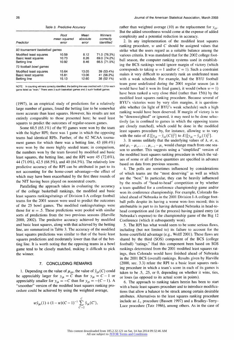
The predictive accuracy of modified least squares was somewhat higher than that of basic least squares, and the predictive accuracy of both was higher than that of the betting line. This could of course simply be a reflection of the limited sample size. Basic least squares has a theoretical advantage over modified least squares-it uses more information- although conceivably this could be offset by the insensitivity of modified least squares to the influence of "outliers." Stern




Table 3. Predictive Accuracy

Root Mean Winners mean squared absolute correctly

Predictor error error identified

93 tournament basketball games Modified least squares 10.59 8.12 71.0 (76.3%) Basic least squares 10.73 8.26 69.0 (74.2%) Betting line 10.92 8.46 66.5 (71.5%) 73 football bowl games Modified least squares 15.64 13.05 39 (53.4%) Basic least squares 15.81 13.06 41 (56.2%) Betting line 15.13 12.60 38 (52.1%)

NOTE: In counting winners correctly identified, the betting line was credited with 1/2 for each game listed as "even." There were 3 such basketball games and 2 such football games.

(1997), in an empirical study of predictions for a relatively large number of games, found the betting line to be somewhat more accurate than least squares. However, his results are not

entirely comparable to those presented here; he used least

squares to predict the outcomes of regular-season games. Some 60.5 (65.1%) of the 93 games were won by the team

with the higher RPI; there was 1 game in which the opposing teams had identical RPIs. Further, of the 62 NCAA tournament games for which there was a betting line, 43 (69.4%) were won by the more highly seeded team; in comparison, the numbers won by the team favored by modified and basic least squares, the betting line, and the RPI were 45 (72.6%), 44 (71.0%), 42.5 (68.5%), and 40 (64.5%). The relatively low

predictive accuracy of the RPI can be attributed in part to its not accounting for the home-court advantage-the effect of which may have been exacerbated by the first three rounds of the NIT having been played on nonneutral courts.

Paralleling the approach taken in evaluating the accuracy of the college basketball rankings, the modified and basic least squares rankings/ratings of Division I-A college football teams for the 2001 season were used to predict the outcomes of the 25 bowl games. The modified rankings/ratings were those for w = .5. These predictions were pooled with similar sorts of predictions from the two previous seasons (Harville 2000, 2002). The predictive accuracy achieved by modified and basic least squares, along with that achieved by the betting line, are summarized in Table 3. The accuracy of the modified least squares predictions was similar to that of the basic least

squares predictions and moderately lower than that of the bet-

ting line. It is worth noting that the opposing teams in a bowl

game tend to be closely matched, making it difficult to pick the winner.

7. CONCLUDING REMARKS

1. Depending on the value of Iijk, the value of Yijk (C) could be appreciably larger for Yijk = C than for Yik = C - 1 or appreciably smaller for Yijk = -C than for yijk = -(C- 1). A "smoother" version of the modified least squares ranking procedure could be achieved by using the weighted average,

C

WYijk(1) +(1-w)(C- )- ijk(C), C'=2

rather than weighted average (10) as the replacement for yijk.

But the added smoothness would come at the expense of added complexity and a potential reduction in accuracy.

2. In any implementation of the modified least squares ranking procedure, w and C should be assigned values that strike what the users regard as a suitable balance among the various criteria. It was mandated that for the 2002 college football season, the computer ranking systems used in establish- ing the BCS rankings would ignore margin of victory (which corresponds to taking w = 1 and/or C = 1). Such a constraint makes it very difficult to accurately rank an undefeated team with a weak schedule. For example, had the BYU football team gone undefeated during the 2001 regular season (as it would have had it won its final game), it would (when w = 1) have been ranked a very close third (rather than 15th) by the modified least squares ranking procedure. Because several of BYU's victories were by very slim margins, it is question- able whether (in light of BYU's weak schedule) such a high ranking would have been deserved. If margin of victory is to be "downweighted" or ignored, it may need to be done selec- tively (as in confined to games in which the opposing teams are closely matched), which could be done in the modified least squares procedure by, for instance, allowing w to vary with the ratio of E{[yijk - Yijk(C)]2} to E{[yijk - Yijk (1)]2

3. It seems unlikely that the underlying values of A, or, a, and I, -i

,.... - , Lc-,I

- -c

would change much from one season to another. This suggests using a "simplified" version of the modified least squares ranking procedure in which the values of some or all of these quantities are specified in advance based on data from previous seasons.

4. The polls are sometimes influenced by considerations of which teams are the "most deserving" as well as which are the "best." In particular, they can be heavily influenced

by the results of "head-to-head" competition or by whether a team qualified for a conference championship game and/or won its conference championship. For example, Colorado finished ahead of Nebraska in the 2001 Division I-A college football polls despite its having a worse won-loss record; this is attributable in part to its having defeated Nebraska in head-to- head competition and (in the process) having gained entry (at Nebraska's expense) to the championship game of the Big 12 Conference (which it subsequently won).

5. The RPI has what would seem to be some serious flaws, including (but not limited to) its failure to account for the home-court/field advantage (e.g., Wolff 2001). These flaws are shared by the third (SOS) component of the BCS (college football) "ratings." Had this component been based on SOS rankings determined from the 2001 modified least squares ratings, then Colorado would have finished ahead of Nebraska in the 2001 BCS (overall) rankings. Results given by Harville (2000, sec. 3.3) relate the RPI to a basic least squares ranking procedure in which a team's score in each of its games is taken to be .5, .25, or 0, depending on whether it wins, ties, or loses (as opposed to its actual score in points).

6. The approach to ranking taken herein has been to start with a basic least squares procedure and to introduce modifications that allow a balance to be struck among certain desirable attributes. Alternatives to the least squares ranking procedure include an L1 procedure (Bassett 1997) and a Bradley-Terry- Luce procedure (Tutz 1986), among others. As in the case of




least squares, the various desirable attributes could be used to evaluate and (as necessary) adapt these procedures for use in the selection or seeding of basketball teams or for use in the BCS ranking procedure.

[Received October 2000. Revised December 2002.]

REFERENCES

Bassett, G. W. (1997), "Robust Sports Ratings Based on Least Absolute Errors," The American Statistician, 51, 99-105.

Harville, D. A. (1977), "The Use of Linear-Model Methodology to Rate High School or College Football Teams," Journal of the American Statistical Association, 72, 278-289.

(1978), "Football Ratings and Predictions Via Linear Models," in Proceedings of the Social Statistics Section, American Statistical Associa- tion, pp. 74-82.

(2000), "The Selection and/or Seeding of College Basketball or Foot- ball Teams for Postseason Competition: A Statistician's Perspective," in Proceedings of the Section on Statstics in Sports, American Statistical Asso- ciation, pp. 1-18.

(2002), "College Football: A Modified Least Squares Approach to Rating and Prediction," in Proceedings of the American Statistical Associ- ation, Section on Statistics in Sports, CD-ROM.

Harville, D. A., and Smith, M. H. (1994), "The Home-Court Advantage: How Large Is It and Does It Vary From Team to Team," The American Statisti- cian, 48, 22-28.

Johnson, N. L., Kotz, S., and Balakrishnan, N. (1994), Continuous Univariate Distributions (2nd ed.), Vol. 1, New York: Wiley.

Leake, R. J. (1976), "A Method for Ranking Teams With an Applica- tion to College Football," in Management Science in Sports, eds. R. E. Machol, S. P. Ladany, and D. G. Morrison, Amsterdam: North-Holland, pp. 27-46.

Stefani, R. T. (1977), "Football and Basketball Predictions Using Least Squares," IEEE Transactions on Systems, Man, and Cybernetics, SMC-7, 117-121.

(1980), "Improved Least Squares Football, Basketball, and Soccer Predictions," IEEE Transactions on Systems, Man, and Cybernetics, SMC- 10, 116-123.

Stern, H. S. (1992), "Who's Number One? Rating Football Teams," in Pro- ceedings of the Section on Statistics in Sports, American Statistical Asso- ciation, pp. 1-6.

(1995), "Who's Number One in College Football?... And How Might We Decide?," Chance, 8, 7-14.

(1997), "How Accurately Can Sports Outcomes Be Predicted?," Chance, 10, 19-23.

Tutz, G. (1986), "Bradley-Terry-Luce Models With an Ordered Response," Journal of Mathematical Psychology, 30, 306-316.

Wolff, A. (2001), "Dirty Pool," Sports Illustrated, March 26, 40-48.



the selection or seeding of college basketball or football teams for postseason competition

Documents