the secondary spectral component of solar microwave bursts

T H E S E C O N D A R Y S P E C T R A L C O M P O N E N T O F S O L A R

M I C R O W A V E B U R S T S

M. S T A H L I * , D. E. G A R Y , and G. J. H U RFO RD

Solar Astronomy, California Institute of Technology, Pasadena, CA 91125, U.S.A.

(Received 15 May, 1989; in revised form 28 August, 1989)

Abstract. Microwave observations in the range 1 to 18 GHz with high spectral resolution (40 frequencies) have shown that many events display a complex microwave spectrum. From a set of 14 events with two or more spectral components, we find that two different classes of complex events can be distinguished. The first group (4 events) is characterized by a different temporal evolution of the spectral components, resulting in a change of the spectral shape. These events probably can be explained by gyrosynchrotron emission from two or more individual sources. The second class (10 events) has a constant spectral shape, so that the two spectral components vary together in intensity. For all ten events in this second class, the ratio of primary to secondary peak frequencies is remarkably similar, exhibiting an average value of 3.4, and both components show a common circular polarization. These properties suggest either a common source for the different spectral components or several sources which are closely coupled. An additional example of this class of burst was observed interferometrieally to provide spatial resolution. This event suggests that the primary and secondary components have a similar location, but that the surface area of the secondary component is larger.

1. Introduct ion

Microwave emission during the impulsive phase of solar flares is generated primari ly

by the gyrosynchrot ron mechanism which involves the interact ion of energetic electrons

with magnetic fields. Spec t roscopy of such emission carries information about the

source parameters , such as the magnetic field, and about the accelerated electrons (e.g.,

Ga ry and Hurford, 1989).

Since 1981, the frequency-agile interferometer (Hurford, Read, and Zirin, 1984) at the

Owens Valley Radio Observa tory (OVRO) has provided solar microwave da ta with

exceptionally high spectral resolut ion in the range 1 to 18 G H z . Solar observat ions were

obta ined with this instrument, first with a single antenna during 1981 and subsequently

using two- and three-element interferometry. Burst observat ions with high spectral

resolut ion were descr ibed by StO.hli, Gary , and Hurford (1989, hereafter Paper I), for

a set of 49 events observed between M a y and October 1981. A m o n g the results of that

phenomenological s tudy was the finding that during some or all of their lifetimes

approximate ly 80~o of the events had complex spectra consist ing of more than one

spectral component . Such a result could not have been obta ined with previous instru-

menta t ion whose spectral resolut ion was limited to A v/v > 5 0 ~ .

In this paper we discuss the mul t icomponent characteris t ics of bursts in more detail,

* Swiss National Science Foundation Fellow from the University of Bern.

Solar Physics 125: 343-357, 1990. �9 1990 Kluwer Academic Publishers. Printed in Belgium.

344 M. STAHLI, D. E. GARY, AND G. J. HURFORD

with emphasis on the relationship between their primary and secondary components*. Of the 49 events discussed in Paper I, we have selected 14 for which the flux of the secondary components was greater than 3 solar flux units (sfu). We also discuss a burst that was observed in 1986 with the OVRO two-element interferometer. The burst was described in detail by Gary and Hurford (1989), and is included here because the spatial information available in the interferometer data allows us to distinguish the two components spatially. In Section 2 we present the observations and the results of the statistical investigation. Some theoretical models are described in Section 3, and discussed in light of the spatially resolved burst observation. Finally, our conclusions are summarized in Section 4.

2. Observations

The observations in 1981 were obtained with a single telescope equipped with a frequency-agile receiver which cycled among 40 frequencies in the range 1 to 18 GHz, first in right- and then in left-circular polarization. A complete sampling of all frequencies in both polarizations required 10 s. Flux densities were compared to an internal noise diode in the receiver which in turn was calibrated against the known flux of Cas A. Details of the observations and calibration are discussed in Paper I. Of the 49 events described in Paper I, 32 bursts showed a multicomponent spectrum at the time of the maximum. Figure 1 shows a typical example of a multicomponent spectrum in which the secondary peak lies at a lower frequency than the peak. High-frequency secondary components are rare, occurring only once in our sample. For a detailed analysis of the secondary peaks, we separated them from the primary component as follows. First a spectral fit of the primary component was made. (For details of the fitting procedure refer to Paper I.) Then the resulting smooth spectrum was subtracted from the observed spectrum. An example of the subtraction of the primary component is shown in Figure 2. The subtraction allows a more accurate measurement of the shape and peak flux of the secondary peaks. Finally, we measured the peak flux, peak frequency, and polarization of the resultant spectrum of the secondary component.

Although there were a total of 32 events showing multicomponent spectra, we limited this study to the 14 bursts whose secondary component exceeded 3 sfu at the time of the maximum (Table I). This was necessary to ensure that the results were not sensitive to measurement and calibration uncertainties. Although some of the events show evidence for more than two spectral components, the additional components were much weaker and difficult to distinguish after subtraction. For the following analysis of multicomponent microwave bursts we restrict ourselves to the primary component and the most intense secondary component.

* In what follows, we will use the term 'component' to refer to a spectral component - that is, a distinguisha- ble peak in the frequency spectrum of the burst. This is not meant necessarily to imply either temporally or spatially separate components. Whenever we refer to temporal or spatial components, we will identify them as such.

THE SECONDARY SPECTRAL COMPONENT OF SOLAR MICROWAVE BURSTS 345

100

ks_ U3

"~ 10 r "

0

X

I,

Fig. 1.

I i i i t i , i I

July 18/81 17:57:30

1 , , ~ , , , , , I 10

F r e q u e n c y ( G H z )

A typical example of a mult icomponent burst spectrum.

TABLE I

Mu l t i componen tOVRO events1981

Event No.

Date Time (UT) Max. flux Peak freq. (sfu) (GHz)

Begin Max. End

1

2 3 4 5 6 7 8 9

10 11 12 13 14

1 July 22 : 51 22 : 52 18 July 17:37 17:38 22 July 20 : 47 20 : 49 24 July 18 : 26 18 : 28 24 July 22 : 41 22 : 42 28 July 16:40 16:41

3 Aug. 20 : 21 20 : 24 4 Aug. 23 : 26 23 : 27

12 Aug. 20 : 55 21 : 06 6 Sept. 21 : 02 21 : 12 8 Sept. 16:58 17:03 8 Sept. 17:42 17:43

28 Sept. 19 : 17 19 : 17 19 Oct. 23 : 06 23 : 27

22 : 54 35 6.8 17 : 40 77 8.3 20 : 51 15 9.1 18 : 36 83 7.7 22 : 53 81 10.8 16:46 41 7.1 20 : 29 240 10.0 23 : 37 17 9.0

>21 : 35 95 10.0 > 2 1 : 2 3 23 7.7 > 17 : 40 74 7.2

17 : 49 20 4.0 19:21 15 5.3

> 23:33 35 8.0

346 M . S T A H L I , D . E . G A R Y , A N D G . J . H U R F O R D

L n n u n I I L I I

10

� 9

o o I, �9 --..' �9 ~/A'sk . ~ ~

c o / ~ X C~

x 1 ~/ ~1 2 i,

I / ~ ~ , , , , ~ , I

1 10

Frequency (GHz) Fig. 2. An example of the technique used for the separation of the two spectral components. The primary peak is fit by a parameterized curve (solid line) which then is subtracted from the observed spectrum (dots).

The remaining flux (triangles with broken line) is due to the secondary component.

2.1. TIME EVOLUTION OF THE TWO COMPONENTS

An important question for understanding the origin of the secondary component is whether both spectral components of a given burst show different temporal behavior. We found that there are two classes of events with multicomponent spectra: ten of our 14 events (70 To) show an essentially identical time evolution of the two spectral components. That is, the shape of their combined spectrum does not change throughout the burst. The remaining four events (numbers 3, 8, 12, and 13 in Table I) show a more complex behaviour whereby the two components do not vary together. In such cases, the combined spectral shape changes significantly during the event. In three of these four events the spectral component that is strongest at the maximum of the event is the weaker of the two earlier in the event. There is some evidence in these four events that the low-frequency component reaches maximum flux earlier than the high-frequency component, but the number of events is too small to allow us to say that this is a general

property of such bursts. The different behaviour of the relative flux of the primary and secondary spectral

components allows us to divide the bursts into two classes. We will see below that members of these classes have other characteristics in common that further strengthen the suggestion that there exist two different classes of complex microwave bursts.


2.2. PEAK FREQUENCIES

The peak frequency distribution of the primary component of the 14 events is shown in Figure 3(a). There is no significant difference between this distribution and that of all 49 events in Paper I. Figure 3(b) gives the histogram for the peak frequencies of the secondary components. This distribution peaks around 2 GHz and shows a rapid fall-off toward higher frequencies.

03 t-

> LJ q..- o

_Q

E Z

Fig. 3.

Main Component

(o)

'I I l 0 , , , , , , , , , , , , , ,

2 4 6 8 10 12 8 ~ - - r - - - "

6

4

2

0 2 4 6 8 10 12

Peak Frequency (GHz) Histograms of the peak frequency distributions of the primary spectral component (a) and the

secondary spectral component (b) using all 14 events in our sample.

(b)

We now consider the role of our selection process on the distribution in Figure 3(b). Spectral peaks below 2 GHz and above 14 GHz are difficult to identify due to calibration uncertainties, which are larger at these frequencies than at intermediate values. Certainly there is evidence for spectral components below 2 GHz in some events, in the form of a rapidly rising low-frequency spectrum, as has been reported by Guidice and Castelli (1975). These are not included in our sample because we could not determine a peak frequency or peak flux. It is also difficult to identify secondary components close to the primary spectral peak, because the two components tend to blend into a single, broader peak. However, in Figure 3(b), the step decrease at higher frequencies cannot be explained by this effect alone. There is only one event (event 12 in Table I) with a high-frequency secondary component, i.e., the peak frequency of the weaker component is higher than that of the primary component. This exception belongs to the group of

348 M. STAHLI, D, E. GARY, AND G. J. HURFORD

events with different time evolution of the two spectral components. In summary then, the selection criteria could account for the absence of secondary components with peak frequencies below 2 GHz, but otherwise the features of the distribution in Figure 3(b) appear to be valid.

A surprising result was found for the ratio of peak frequencies of the primary and secondary spectral components. Most of the events have a ratio between 3 and 4, which suggests a correlation between the two frequencies (see Figure 4). If we eliminate the

c- �9 >

LIA

O k_ �9 n 2 8

Z

0 1 2 3 4 5

Peok Frequency Rotio

Fig. 4. Histogram of the peak-frequency ratios, i.e. the ratios of the primary component peak frequency to the secondary component peak frequency, for all events. The four events with a different time evolution

of the two spectral components are hatched.

four events with different time evolutions of the two components (hatched areas in Figure 4) the result is even more striking. The correlation also can be seen in Figure 5, which plots the frequency of the primary component against that of the secondary component. When the four events belonging to the one class of temporal behaviour (marked with circles) are excluded, the average frequency ratio found for the remaining 10 events of the other class is 3.4 + 0.3, as shown by the dashed line.

In agreement with the results from the larger set of bursts reported in Paper I, the peak frequencies stay remarkably constant throughout the evolution of a burst. In our sample of 14 multieomponent events, the primary peak of only 4 of the bursts shows a significant frequency shift (about 10-15 ~o), whereas no shift of the secondary peaks is seen in any of the 14 events. However, the frequency resolution of the Owens Valley instrument between 2 and 3 GHz is only about 10~o, so that we can only set an upper limit of

10~o to any spectral shift of the secondary components with time.

T H E S E C O N D A R Y S P E C T R A L C O M P O N E N T OF SOLAR M I C R O W A V E B U R S T S 349

! (9 ~ 1 0

>.., 0 (.-

c r

h_ xl Ul �9

a._

-~ 5 c- O) r

o r

E o

O t'-

i i i

/

/

/ / x

• |

x/ ~t

X /

/ / |

/ /

/ /

/ /

' I ' ' ' ' I

|

0 ~ , , , I ~ , , , I

0 5 10

Secondory Component Peok Frequency (GHz)

Fig. 5. Relation between the peak frequencies of the primary component and the secondary component. The four events with different time evolution of the two spectral components are circled. The remaining ten

events have a peak-frequency ratio of 3.4 + 0.3 (broken line).

2.3. FLUX DENSITY RATIO AND SPECTRAL SHAPE

The flux density ratio of the two spectral components shows more variation than the peak frequency ratio as shown in the histogram of Figure 6. On average, the flux density of the secondary component at the time of maximum of the burst is about a factor of 8 lower than that of the primary component. The 4 events with different time evolution tend to have a smaller flux density ratio of 2-4, and the ratio can even reverse during the burst, as mentioned earlier.

Since the flux ratio of the 10 events with the common time evolution of the two components is fixed, the spectral shape does not vary appreciably with time for these events. A 'typical' spectral shape for these 10 events was found by averaging the spectral fit parameters for the events. The resulting slopes on the low- and the high-frequency side of the primary component spectra agree with the values for the larger sample of bursts in Paper I. The data are summarized in Table II. The high-frequency slope of the secondary component is quite inaccurate, however, because usually there were only few data points in this part of the spectrum.

2.4. POLARIZATION

Significant polarization for both spectral components was noted in only 7 of the 14 events. In other cases reliable polarization measurements for the secondary component could not be obtained because the polarization is determined from the subtraction of

350 M. ST,~HLI, D. E. GARY~ AND G. J. HURFORD

' [ ' ' I

03 [.- �9 >-

Ld

'S

...(3

E Z

0 r r i I 1

0 10 15

g~4~ ......... ~ , ~

N 5

Fig. 6. Histogram of the peak flux ratios. The four events with a different time evolution of the two spectral components are hatched.

TABLE II

Typical multicomponent spectrum

Secondary component Primary component

LF slope 3.1 + 0.3 3.0 + 0.3 HF slope -5 .5 + 0.9 - 2 . 9 + 0.3 Peak frequency (GHz) 2.5 + 0.2 8.4 + 0.5 Peak flux (sfu) 10 _+ 3 75 + 20

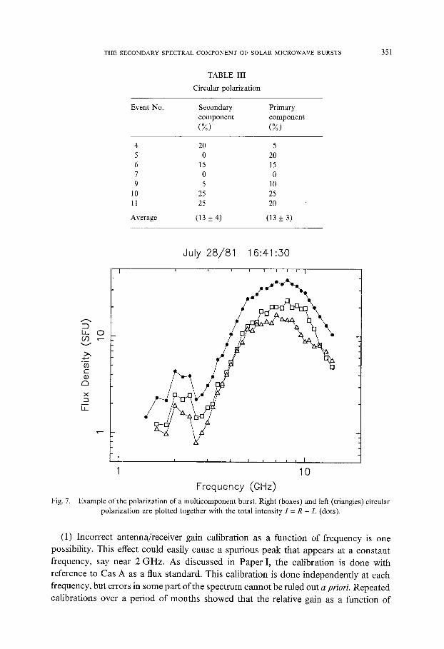
two sometimes weak spectral features. The polarization data are summarized in Table III with Figure 7 showing an example. Primary and secondary peaks are both slightly polarized in the same sense, with the exception of one event that is unpolarized. The average percent polarization is (13 + 4 ) ~ and there is no significant difference in polarization between the two spectral components.

2.5 . POSSIBLE I N S T R U M E N T A L EFFECTS

Before discussing conclusions based on these observations, it is important to consider whether the secondary spectral components could be attributed to instrumental effects, especially in view of the remarkable constancy of the ratio of peak frequencies displayed in Figures 4 and 5. We now discuss two possible effects.

T H E S E C O N D A R Y S P E C T R A L C O M P O N E N T O F S O L A R M I C R O W A V E B U R S T S 351

TABLE III

Circular polarization

Event No. Secondary Primary component component (%) (%)

4 20 5 5 0 20 6 15 15 7 0 0 9 5 10

10 25 25 11 25 20

Average (13 • 4) (13 • 3)

July 28/81 16:41:,..30

Fig. 7.

I i i i i i i i i I

A

LL. 0

E

r'~

X

b_

l i i i ~ i i I I

10 Frequency (GHz)

Example of the polarization of a multicomponent burst. Right (boxes) and left (triangles) circular polarization are plotted together with the total intensity I = R + L (dots).

(1) Incorrect antenna/receiver gain calibration as a function of frequency is one

possibility. This effect could easily cause a spurious peak that appears at a constant

frequency, say near 2 GHz. As discussed in Paper I, the calibration is done with

reference to Cas A as a flux standard. This calibration is done independently at each

frequency, but errors in some part of the spectrum cannot be ruled out a priori. Repeated

calibrations over a period of months showed that the relative gain as a function of

352 M. STAHLI, D. E. GARY, AND G. J. HURFORD

frequency was constant to within measurements errors, with any given gain variations affecting only the overall normalization of the spectra. Therefore, a frequency-dependent gain should show up as a spectral peak in the affected frequency range for all events. If this were the case, however, such peaks should be visible in the preflare background spectrum that is subtracted from each burst. We examined the preflare spectra and found them to be smooth to within about 10~/o. Furthermore, the same relative gain calibration used in this paper was used for all 49 bursts presented in Paper I. For the 49 events, some events with secondary spectral components were bracketed by observations of other, single-component events which did not exhibit corresponding features. Furthermore, some events showed a secondary component for only part of their lifetimes. We, therefore, rule out the possibility that the secondary components are a spurious result of calibration errors.

(2) A second possibility is the appearance of bogus spectral features associated with the finite rate of frequency switching of the frequency-agile receivers. As mentioned earlier, observing frequencies are tuned in a cycle in which the spectrum is sampled in right-hand (RH) polarization for 5 s, then in left-hand (LH) polarization, taking an additional 5 s. If the flux changes abruptly within the 5 s that the spectrum is sampled, this might appear as a spurious spectral feature, particularly in the polarization spectrum. In fact, a few of the original 49 bursts studied in Paper I showed this effect at times, but such events have been excluded from the 14 events we discuss in this paper. We believe that none of the present 14 events were affected by this because (i) we included no rapidly varying or short duration events in the sample, (ii) the secondary components are present with nearly constant peak frequency in many consecutive 10 s measurements of the spectrum, (iii)the secondary components are present in both polarizations.

Finally, independent evidence for the reality of the secondary components is given in the next section, where we describe a burst that has a secondary spectral component with many of the characteristics we have been describing but which was observed with different instrumental and calibration techniques.

We conclude that the secondary spectral components are neither due to nor affected by any known instrumental effect.

3. Discussion

Our investigation of the spectral characteristics of solar microwave bursts has shown that most events have complex spectra. This result alone may not seem surprising, since from optical observations we know that many solar flares have complicated sources, consisting of several individual kernels. Indeed, radio-imaging observations such as with the Very Large Array sometimes exhibit multiple sources during a burst (e.g., Kundu, Schmahl, and Velusamy, 1982). However, single-frequency imaging observations more typically show single sources with simple structure near the peak of a burst (e.g., Marsh and Hurford, 1980; Velusamy and Kundu, 1982). It is only when images are made simultaneously at two or more frequencies that these divergent views can be reconciled, for then the sources, while remaining spatially simple at each frequency, sometimes are


found to have different morphologies and locations at different frequencies (Shevgaonkar and Kundu, 1985; Dutk, Bastian, and Kane, 1986). This suggests that, at least for some flares, different parts of the microwave spectrum come from different sources. If these 'microwave kernels' were to have significantly different parameters, such as magnetic field, electron density and source size, it could well be possible for spatially-integrated microwave spectra to display more than one peak. Such a model probably could explain the four events that show differences in the time evolution of the two spectral components.

The majority (10 our of 14) of the events in our sample of events with complex spectra, however, show a good temporal correlation between the primary and secondary spectral components. Other properties of this class of events are that the spectral components are related by a common frequency ratio and by a common polarization. These properties suggest that the emission may come from a single source or from sources that are strongly coupled. In the following we briefly consider three models for this class of event.

3 . 1 . H O M O G E N E O U S S O U R C E

Gyrosynchrotron emission from a single source could result in a microwave spectrum with secondary components at low frequencies if the magnetic field strength and direction is sufficiently homogeneous. Theoretical calculations of microwave emission (e.g., Klein, 1987; MacKinnon etal., 1986) show that in addition to high-frequency emission which comes from harmonics > 10 of the gyrofrequency, under some cir- cumstances one might expect low-frequency, subsidiary peaks from gyroresonance emission at the lowest few discrete harmonics as well. Such an explanation for the observed secondary spectral components has the advantage that the emission arises from a single population of electrons, and so can easily explain the common temporal evolution of the two spectral components. In addition, a moderate degree of circular polarization in the same sense would be expected for the two spectral components. The main disadvantage of this explanation, however, it that it requires a homogeneous source, since inhomogeneities would blend the gyroresonanee lines so that the spectral fine structures at low harmonics would disappear. Other workers such as Dulk and Marsh (1982) have purposely averaged over the lowest harmonics of the gyrofrequency to obtain their plots of effective temperature because they felt such homogeneous magnetic fields were unlikely to be found in the Sun. The steep low-frequency slopes seen in high-resolution spectra (see Table II and Paper I), however, might be taken as evidence that some sources are fairly homogeneous, since gradients in source parameters will flatten the low-frequency slopes. In summary, then, while it is possible that spectral structure is a consequence of discrete harmonics, such an explanation would require a degree of source homogeneity for which we do not yet have definitive evidence.

3.2. I N H O M O G E N E O U S S I N G L E L O O P

We now consider a model with a single inhomogeneous source. M~itzler (1978) was among the first to show that a single flaring loop can produce a complex spectrum. In his treatment, two spectral peaks are defined by the low magnetic field at the top of a

354 M. ST~,HLI, D. E. GARY, AND G. J. HURFORD

loop and the higher magnetic field near the footpoints. As shown in M~itzler's Figure 4, his model can give a common sense of circular polarization for the two spectral components. Also in agreement with our observations, his model would suggest a common temporal evolution for the two spectral components since both would arise from a common population of electrons in a single magnetic loop. Between the spectral peaks, his calculations showed a relatively flat spectrum with spectral index < 2 due to optically thick radiation from a distribution of sources whose combined area decreases with increasing frequency. In contrast to this, however, our data show a primary component with a fairly steep low-frequency slope, characteristic of a more limited range of source sizes than suggested by the M~ttzler model.

An alternate geometry that might be considered is a single, asymmetric loop with a low magnetic field near one footpoint and a high field near the other. The two spectral components again come from two locations in the loop, in this case, one near each footpoint. Such a geometry is discussed by Kundu and Vlahos (1979). Since the radiation is produced by a common population of electrons, good temporal correlation would be expected for the two resulting spectral components. However, in such a model we would expect opposite circular polarization of the two components, which is not observed. The observed constant frequency ratio of 3.4 cannot be explained in an obvious manner with either of these geometries for a single inhomogeneous loop.

3.3. O T H E R M A G N E T I C F I E L D C O N F I G U R A T I O N S

Another possibility for the generation of microwave radiation with a complex spectrum is a source consisting of several loops, either nested, or in the form of an arcade of adjacent loops. In order to have common temporal profiles for the two spectral components, the loops must be magnetically coupled. In this case, nested loops have the advantage that a common polarization might be expected, whereas for adjacent loops, both opposite and common senses of circular polarization might be possible. Dulk and Dennis (1982) discussed the spectrum of radio emission expected from a nested loop geometry with a continuous gradient of parameters. Their motivation was to explain spectral slopes, observed in low resolution spectra, that were shallower than expected from theory. In Paper I, we saw that the shallower slopes were an artifact of the presence of the secondary components and low resolution observations. Nevertheless, parameter gradients with a more discrete character than the continuous gradient assumed by Dulk and Dennis could provide the basis for an explanation of the multiple spectral components. It is tempting to speculate that if this were the case, the constant frequency ratio of 3.4 might be a result of parameter gradients whose distribution is related to stability conditions for the nested magnetic loops.

3.4. A SPATIALLY-RESOLVED BURST

One approach to distinguishing among the various possibilities outlined in the foregoing discussion is to determine the relative locations of the primary and secondary spectral components. This was not possible for the 1981 data since only a single antenna was equipped with frequency-agile receivers. By 1986, however, interferometric data was

THE SECONDARY SPECTRAL COMPONENT Ot: SOLAR MICROWAVE BURSTS 355

available so as to provide spatial resolution for bursts in one dimension. One such event

is described in detail by Gary and Hurford (1989, Paper II), where it was noted, but not discussed, that a minor secondary spectral component was present at low frequencies.

Figure 8(a) taken from Paper II shows the total power spectrum at a time when the secondary component is quite apparent near 4.5 GHz. The solid and dashed curves are

10 10

L 03 v

1

O IX.

O b--

0.1

, i , , i , , ]

18:5:40 x x

O 0 , / •

70

Frequency (OHz)

> 1 4-J

-6 0s

0.1

oo

..c 0_

18: 4 : 0

• [ ]

0

,::]:i',:]::::]:::: 560

, , , I , t , , I ~ , , , I ' ~ ' ' 0

5 10 15 20

Frequency (GHz)

Fig. 8. Data from a spatially-resolved burst that occurred on 1986 February 3. (a)The total power spectrum in right-hand (crosses) and left-hand (boxes) circular polarization, with the primary component fit by a thermal spectrum. A secondary spectral component appears near 4.5 GHz. (b) The corresponding

relative visibility and phase as a function of frequency.

fits to the primary component of thermal microwave spectra from a homogeneous source in right- and left-hand polarization. Although the secondary component has a peak frequency of 4.3 GHz, which is higher than that of any of the bursts in our sample, the primary component also has an unusually high frequency, so that the ratio of peak frequencies is 2.9 - not too different from the value of 3.4 + 0.3 found for our 1981 sample. In addition, the time behaviour of the primary and secondary components was

similar. Having established that this event belongs in the same class as the 10 bursts in our 1981 sample that show similar time behaviour of the two components, we now turn to its spatial characteristics.

As discussed in Paper II, the primary component of this burst (above 6 GHz) was simple by two observational criteria: (1)the interferometric phases showed a linear dependence on frequency, which implies that the source is at the same (one-dimensional) location at each frequency and (2) the relative visibility (the ratio of correlated amplitude

356 M. STAHLI, D. E. GARY, AND G. I. HURFORD

to total power) had a simple dependence on frequency that matched that expected for a relatively small (5-10 arc sec) source of gaussian cross-section. The relative visibility and phase, now extended down to 4 GHz to include the secondary component, are shown in Figure 8(b) and 8(c), respectively. We see that the phase data exhibit the same linear dependence on frequency in the range 4-6 GHz as at higher frequencies. This means that the secondary component has the same location as the primary component.

The relative visibility shown in Figure 8(b), however, decreases at frequencies below 6-7 GHz, indicating that the secondary component has a larger source size than the primary component. The one-dimensional source size derived for the secondary spectral component at 4.5 GHz is 17 arc sec for the time shown in Figure 8(a), which is some 4 times the FWHM diameter of the primary component at that time (see Paper II).

Before we can fully interpret the interferometric results, three caveats should be mentioned. First, the interferometric data were obtained for only a single event, which leaves open the possibility that other events of this class have different spatial characteristics. Second, the spatial information for this event is in one dimension only. There could be a difference in the source position of the two components along the direction of the fringes. Third, this was quite a weak event, which tends to enhance the sensitivity of the result to preflare subtraction and which may also influence the degree to which this event might be considered as typical.

The fact that the low-frequency, secondary component in this event is at the same location but has a larger source size than the primary component seems most consistent with the nested loop model. The homogeneous source model would also predict a common location for the two components as was observed, but would also predict a similar source size which was contrary to the data for this event. Thus, while the event is most consistent with the nested loop model, additional observations combining high spectral and spatial resolution are required to firmly establish the correct interpretation.

4. Conclusions

Microwave bursts with complex spectra, consisting of two or more spectral components, can be divided into two classes. One class (4 of the 14 events) may result from bursts in which the microwave radiation is generated in two different gyrosynchrotron sources that evolve differently in time. This conclusion is based on the observation that the temporal evolution of the spectral components is independent. Confirmation of this suggestion will require spatially-resolved observations of bursts of this class.

A second class of microwave bursts with complex spectra is characterized by a common temporal evolution of the spectral components, i.e. a constant shape of the spectrum throughout the event. Additional properties of this class are the similarity of the circular polarization of both components and the remarkable commonality in the ratio of primary peak to secondary peak frequencies from event to event. These properties suggest that the two components originate in a common source or from individual sources that are strongly coupled. One additional burst, observed with one-dimensional spatial resolution, could be identified as a member of this class. The spatial information


indicated that the secondary component was larger than the primary component, but shared a common centroid location. This would seem to be the most consistent with a model whereby both components originate within a set of nested loops. A facet of the data that is not understood at present is the constancy and value of the ratio of peak frequencies of the two components.

Acknowledgements

We gratefully acknowledge helpful discussions with Dr H. Zirin. The work was sup- ported by NSF grants ATM-8610330 and AST-8702682 and by NASA NAG 5-946 to the California Institute of Technology. This study was carried out while one of the authors (MS) was a visiting scientist at the California Institute of Technology with a fellowship from the Swiss National Science Foundation.

References

Dulk, G. A. and Dennis, B. R.: 1982, Astrophys. J. 260, 844. Dulk, G. A. and Marsh, K. A.: 1982, Astrophys. J. 259, 350. Dulk, G. A., Bastian, T. S., and Kane, S. R.: 1986, Astro_phys. J. 300, 438. Gary, D. E. and Hurford, G. J.: 1989, Astrophys. J. 339, 1115. Guidice, D. A. and Castelli, J. P.: 1975, Solar Phys. 44, 155. Hurford, G. J., Read, R. B., and Zirin, H.: 1984, Solar Phys. 94, 413. Klein, K.-L.: 1987, Astron. Astrophys. 183, 341. Kundu, M. R. and Vlahos, L.: 1979, Astrophys. J. 232, 595. Kundu, M. R., Schmahl, E. J., and Velusamy, F.: 1982, Astrophys. J. 253, 963. MacKinnon, A. L., Costa, J. E. R., Kaufmann, P., and Dennis, B. R.: 1986, Solar Phys. 104, 191. Marsh, K. A. and Hurford, G. J.: 1980, Astrophys. J. 240, Ll11. M/itzler, C.: 1978, Astron. Astrophys. 70, 181. Shevgaonkar, R. K. and Kundu, M. R.: 1985, Astrophys. J. 292, 733. St/ihli, M., Gary, D. E., and Hurford, G. J.: 1989, Solar Phys. 120, 351. Velusamy, F. and Kundu, M. R.: 1982, Astrophys. J. 258, 388.

the secondary spectral component of solar microwave bursts

Documents