Policy Research Working Paper 9464

The Rural-Urban Divide and Intergenerational Educational Mobility in a Developing Country

Theory and Evidence from Indonesia

Md Nazmul Ahsan M. Shahe Emran

Forhad Shilpi

Development Economics Development Research GroupNovember 2020

Pub

lic D

iscl

osur

e A

utho

rized

Pub

lic D

iscl

osur

e A

utho

rized

Pub

lic D

iscl

osur

e A

utho

rized

Pub

lic D

iscl

osur

e A

utho

rized

Produced by the Research Support Team

Abstract

The Policy Research Working Paper Series disseminates the findings of work in progress to encourage the exchange of ideas about development issues. An objective of the series is to get the findings out quickly, even if the presentations are less than fully polished. The papers carry the names of the authors and should be cited accordingly. The findings, interpretations, and conclusions expressed in this paper are entirely those of the authors. They do not necessarily represent the views of the International Bank for Reconstruction and Development/World Bank and its affiliated organizations, or those of the Executive Directors of the World Bank or the governments they represent.

Policy Research Working Paper 9464

This paper provides an analysis of the rural-urban divide in intergenerational educational mobility in Indonesia with two distinguishing features. First, the estimating equa-tions are derived from theory incorporating rural-urban differences in returns to education and school quality, and possible complementarity between parent’s education and financial investment. Second, the data are suitable for tack-ling the biases from sample truncation due to coresidency and omitted cognitive ability heterogeneity. The evidence rejects the workhorse linear intergenerational educational persistence equation in favor of a convex relation in rural and urban Indonesia. The rural-urban relative mobility curves cross, with the children of low educated fathers enjoying higher relative mobility in rural areas, while the pattern flips in favor of the urban children when the father has more than nine years of schooling. However,

the rural children face lower absolute mobility across the whole distribution of father’s schooling. Estimates from the investment equation suggest that, in urban areas, children’s peers are complementary to financial investment by par-ents, while the adult role models are substitutes. In contrast, separability holds in villages. Peers and role models are not responsible for the convexity in both rural and urban areas, suggesting more efficient investment by educated parents as a likely mechanism, as proposed by Becker et al. (2015, 2018). The theoretical relation between the intercepts of the mobility and investment equations helps in understand whether school quality is complementary to or a substitute for parental financial investment. This paper finds evidence of substitutability, implying that public investment to improve the quality of rural schools is desirable on both equity and efficiency grounds.

This paper is a product of the Development Research Group, Development Economics. It is part of a larger effort by the World Bank to provide open access to its research and make a contribution to development policy discussions around the world. Policy Research Working Papers are also posted on the Web at http://www.worldbank.org/prwp. The authors may be contacted at fshilpi@worldbank.org.

The Rural-Urban Divide and Intergenerational Educational Mobility in aDeveloping Country: Theory and Evidence from Indonesia

Md Nazmul Ahsan1

Saint Louis University

M. Shahe EmranIPD, Columbia University

Forhad ShilpiWorld Bank

Keywords: Intergenerational Educational Mobility, Rural-Urban Divide, complemen-tarity, Convexity, Returns to Education, School Quality, Peer and Role Model Effects,Coresidency, Sample Truncation, Ability Heterogeneity

JEL Codes: J62, O12

1We would like to thank Hanchen Jiang for helpful discussions. Emails for correspondence: ah-sanm@slu.edu, shahe.emran.econ@gmail.com, fshilpi@worldbank.org. Standard disclaimers apply.

(1) Introduction

Economic liberalization in the 1980s and 1990s resulted in increasing inequality in many

developing countries (World Development Report 2006). Intra-country spatial inequality

also increased in most cases, with an increasing gap in living standards between rural and

urban households (Kanbur and Venables (2005)).2 Using Demographic and Health Survey

(DHS) data on 65 countries, Young (2013) finds that rural-urban inequality accounts for

40 percent of the mean country inequality and much of the cross-country variation. To

what extent the observed inequality is due to the roots of intergenerational persistence

in economic status is an important question for the policymakers. It is thus surprising

that there is little research on the rural-urban differences in intergenerational mobility in

developing countries. Most of the existing studies focus exclusively on urban areas, and a

comparative analysis of rural vs. urban areas remains relatively unexplored.3

We provide a theoretically grounded empirical analysis of the rural-urban divide in

intergenerational educational mobility in Indonesia in the 1990s and 2000s.4 Inequality in

Indonesia increased dramatically over this period: the consumption Gini rose from 29.2 in

the 1990s to 38.9 in the 2000s. There are important rural-urban differences: inequality is

lower in the rural areas, and the rise in inequality from the 1990s to 2000s has also been less

pronounced compared to the urban areas (Kanbur and Jhuang (2014)). A link between

higher inequality and lower intergenerational mobility has been the focus of a growing

literature on the Great Gatsby Curve (Corak (2013), Fan et al. (2020), Neidhofer et al.

(2018)). Does the higher level of inequality in the urban areas imply that there is a “rural

bias” where urban children face lower educational (and economic) mobility compared to

2In Indonesia, the rural-urban gap in per capita monthly household expenditure increased from 12,991rupiahs in 1984 to 18,005 rupiahs in 1996 (deflated by food price deflator, see Friedman (2005)). Therural-urban divide has been the focus of a long literature in development economics, from Lewis model toKuznet’s inverted-U process of inequality, to political economy analysis highlighting “urban bias” (Lipton(1975))) in public goods allocation and “price scissors” (Sah and Stiglitz (1987)) designed to extract surplusfrom the rural areas in the 1960s and 1970s.

3Among the few available studies, see Iversen et al. (2017) on rural-urban differences in occupationalmobility, and Emran and Shilpi (2015), and Asher et al. (2018) on rural-urban educational mobility inIndia. However, the estimating equations in these studies are not derived from a theoretical model.

4The focus on education is motivated primarily by the role played by skill premium in rising inequality,and an emphasis on educational mobility as the key to tackling economic inequality (Goldin and Katz(2008), Stiglitz (2012), Autor (2014)).

1

the rural children, as the logic of the Great Gatsby Curve seems to suggest?

The empirical analysis is based on the estimating equations derived from an extension

of Becker et al. (2015)’s model to incorporate the rural-urban differences in returns to

education and school quality. The close link between the theory and empirical work allows

us to explore the economic mechanisms in a consistent manner which distinguishes this

paper from much of the existing literature on intergenerational educational mobility in

developing countries.5 The returns to education are usually higher in the urban areas

because the manufacturing and services activities are more skill intensive and may give rise

to agglomeration externalities.6 Similar to the classic analysis of Becker and Tomes (1986)

and Solon (2004), higher returns to education for parents strengthen the impact of family

background on children’s educational opportunities in our model. The recent evidence on

Indonesia shows that the rural schools remain at a substantial disadvantage in terms of

teacher quality, teacher absenteeism, and school infrastructure during our study period

(see World Bank (2016), Echazarra and Readinger (2019)).7 An important policy question

in this regard is whether public investment in rural schools would be effective in improving

intergenerational mobility. As discussed by Becker and Tomes (1986), and Becker et al.

(2015), the equity and efficiency effects of public educational investment depend critically

on whether it is complementary to or a substitute for private educational investment by

parents, and understanding the nature of this interaction is an important goal of our study.

The theoretical model delivers a quadratic estimating equation for intergenerational

mobility similar to that of Becker et al. (2015)), with the linear conditional expectation

function (CEF) widely used in the current literature as a special case.8 Following Becker

et al. (2015, 2018), an important feature of the model is complementarity of parent’s ed-

5Our model is different from that of Becker et al. (2015) in terms of the nature of the credit marketimperfections. Becker et al. (2015) assume that the poor parents pay a higher interest rate for educationalloans, but they can borrow as much as needed. Following Becker and Tomes (1986) and Solon (2004), weassume that there is no credit market for financing education of children, and the parents pay from theirown income. We believe that, in the context of developing countries, our assumption is more realistic.

6For evidence of higher skill intensity in urban Indonesia, see World-Bank (2016).7In Indonesia, the roots of urban bias in school quality go back to the Dutch colonial policies that

allocated most of the educational budget to urban schools catering to the children of elite Dutch andChinese households, and the rural schools (desa schools) were neglected (Frankema (2014)).

8All of the published empirical studies on intergenerational educational mobility we are aware of estimatea linear conditional expectation function (CEF).

2

ucation with financial investment in the education production function of children. This

complementarity may reflect peer and role model effects in addition to more efficient in-

vestment by educated parents, and can give rise to a convex CEF. Unlike the standard

linear model, relative mobility in our model depends on parent’s schooling level, and the

urban and rural relative mobility curves can cross. The approach developed in this paper

is of wider interest as it can be applied to household survey data from other developing

countries.

For the empirical analysis, we take advantage of the rich household panel data from the

Indonesia Family Life Survey (IFLS) to make progress on two major issues highlighted in the

literature: (i) truncation bias due to coresident sample, and (ii) omitted variables bias due

to ability heterogeneity. An important data constraint on the analysis of intergenerational

mobility in developing countries is truncation bias caused by coresidency restrictions in

defining household membership in surveys (see Emran et al. (2018)). The IFLS data do

not suffer from any significant truncation as the survey collected information on nonresident

parents of any household member older than 15.9 A second important advantage of the IFLS

2014 data used in this paper is that good quality measures of cognitive ability are available

which allows us to control for ability heterogeneity across children in the regressions. Our

main analysis of intergenerational mobility is based on the 18-40 years old children in the

2014 wave of IFLS who went to school in the 1990s and 2000s. We use the earlier rounds

of the panel data (1993, 1997, 2000, 2007) to understand the effects of parent’s education

on financial investment in children’s schooling. Another important part of our empirical

analysis is the estimates of returns to education at the household level in rural vs. urban

areas.10 The availability of 5 rounds of panel data on household consumption expenditure

allows us to provide estimates for both the parental and children’s generations.

The main conclusions from the empirical analysis are as follows. First, the CEF is

convex in both rural and urban Indonesia, rejecting the work-horse linear model used in the

existing literature. The estimates of relative mobility show contrasting rural-urban pattern:

9For a discussion on the advantages of the IFLS data for studying intergenerational mobility in Indonesia,see Mazumder et al. (2019).

10The returns to education here relate to a household’s permanent income, not only the labor marketreturns in a given year as is the case in the Mincerian literature. See below the discussion in section (6.1).

3

while the children from low educated households enjoy higher relative mobility in the rural

areas, the pattern flips at the right tail of father’s education distribution, with 9 years of

father’s schooling as the bifurcation point. The pattern of relative mobility is thus much

more nuanced than the simple negative relation between inequality and mobility posited in

the Great Gatsby Curve. The rural children, however, face lower absolute mobility across

the distribution of parental schooling.11 The evidence shows that returns to education

measured in terms of household income are higher in the urban areas, and this is true for

both the parent’s and children’s generations. Higher returns to education in the parent’s

generation seem to be an important factor underlying the observed higher intergenerational

schooling persistence in the urban areas. The estimates of the intercepts of the mobility

and investment equations provide strong evidence in favor of the hypothesis that parental

investment is a substitute for school quality in Indonesia. This suggests that government

expenditure to improve school quality in rural Indonesia is likely to be an effective policy

tool on both equity and efficiency grounds.

Our analysis of the sources of convexity in the mobility CEF shows that peer effect is

complementary to parental investment in the urban areas, but it is not responsible for gen-

erating the convexity in the mobility equation. In the rural areas, the interaction between

peer effect and financial investment is not significant, suggesting separability. Better edu-

cated peers weaken the impact of family background on children’s educational attainment

in both the urban and rural areas. The role models, in contrast, are substitutes of financial

investment in the urban areas, and separable in the rural areas. Similar to the peer effect,

better educated role models weaken the impact of father’s education on children’s schooling

attainment, both in rural and urban areas. It is important to appreciate that the empirical

conclusions discussed in this paper are unlikely to be driven by biases arising from hetero-

geneity in cognitive ability, as we control for quadratic effects of children’s cognitive ability

in all the regressions.

The extended Becker-Tomes model provides an explanation for these contrasting effects

of peers and role models in the investment vs. mobility equations where the degree of

11This is in sharp contrast to the conclusion one gets from the standard linear model. The estimatesfrom the linear CEF implies that all rural children enjoy higher relative mobility.

4

diminishing returns to financial investment in the education production function plays a

critical role. The evidence that peer and role model effects do not generate the convexity

in the mobility equation suggests more efficient investment by educated parents as a likely

source of convexity as emphasized by Becker et al. (2015, 2018).

The rest of the paper is organized as follows. Section (2) provides a brief discussion on

the related literature with a focus on work on developing countries, and on Indonesia in

particular. Section (3) develops the extension of the Becker et al. (2015) model with self-

finance constraint on financing children’s education and derives the estimating equations

for intergenerational persistence and optimal parental investment. Section (4) discusses the

data with a focus on the issues of sample truncation due to coresidency and the construction

of a cognitive ability index using three measures of ability in IFLS 2014. The next section

presents the estimates for the mobility equation. Section (6) is devoted to understanding

the economic forces at work behind the rural-urban divide in educational mobility. Section

(7) explores the role of peer and role model effects in the convexity of mobility equation.

The paper concludes with a summary of the results and highlights the portability of the

model and methods developed here to other developing country analysis.

(2) Related Literature

The literature on intergenerational economic mobility in developed countries is vast,

with fundamental theoretical and empirical contributions, from Becker-Tomes (1979, 1986),

to Solon (1992), to Chetty et al. (2014) are some of the seminal studies. Most of the studies

focus on intergenerational persistence in permanent income between father and son. An

important finding from this literature is that rich panel data on income for many years from

appropriate phases of the life-cycle are required to get credible estimates of intergenerational

persistence in permanent income (Solon (1992), Mazumder (2005)). For excellent surveys

of this literature see, Solon (1999), and Black and Devereux (2011).

The literature on developing countries is limited, with increasing interest in the last

few years (see Iversen et al. (2019) and Emran and Shilpi (2019) for recent surveys). The

required panel data on income are not available in most of the developing countries, and as

a result, the focus of the literature has been on educational linkages across generations (see,

5

among others, Neidhofer et al. (2018), Azam and Bhatt (2015), Emran and Shilpi (2015),

Hertz et al. (2008), Thomas (1996)). Among the few contributions on income mobility, see

Fan et al. (2020) on China. The recent analysis of intergenerational occupational linkages

in developing countries includes Bossuroy and Cogneau (2013), Emran and Sun (2015) and

Emran and Shilpi (2011).

The literature on intergenerational mobility in Indonesia is small, with only a hand-

ful of studies available. We are aware of three studies on Indonesia that can be broadly

classified as dealing with intergenerational issues in education, and all of them study the

effects of the same policy experiment: a large scale school construction program in the

1970s, originally studied by Duflo (2001).12 Hertz and Jayasundera (2007) analyze the

effects on IGRC in schooling for the children, and find that the exposure to new schools

weakened the intergenerational persistence for men, but not for women. In a recent paper,

Mazumder et al. (2019) focus on the long-term effects of the program on the second gen-

eration children, i.e., children of those who benefited from the school construction when

they were children themselves. Since most of these second generation children have not

completed their schooling, it is difficult to estimate IGRC in schooling attainment. They

thus focus on the academic performance of the children which would be correlated with

the final educational attainment of a child. They show that the children of the mothers

exposed to the large scale school construction in the 1970s had significant gains in school

examination scores. But they do not find any effects of the fathers. In a related paper,

Akresh et al. (2018) study the effects of school construction on the socioeconomic well-being

of the first generation directly exposed to the program and the intergenerational effects on

school attainment using the SUSENAS 2016 cross section data.

(3) Rural vs. Urban: A Model of Intergenerational Educational Mobility

We consider an economy consisting of two-person households with the parent and a

child. The parent of child i has education level Epi (years of schooling). Following Solon

12The main impact of the program was on the cohorts who went to school in the early 1970s.

6

(2004) and Becker et al. (2015, 2018), parent’s income is determined as follows:

Y pi = Y pj

0 +RpjEpi (1)

So the returns to education is Rpj in the parental generation in location j = r, u, with

r for rural and u for urban. We assume that the parents with zero year of schooling earns

Y p0 > 0. The focus here is on how the household permanent income changes with the

education of the parent Epi . The “returns to education” here thus refer to a household’s

permanent income, not an individual’s labor market income in the survey year which has

been the focus of the Mincerian literature on returns to education.

The parent allocates income Y pi between own consumption Cp

i and investment in the

child’s education Ii. The budget constraint is:

Y pi = Cp

i + Ii (2)

An important assumption in this specification of the budget constraint is that there is

no credit market where the parents can borrow to finance children’s education. This is a

plausible assumption in the context of developing countries where the student loan market

(public or private) is underdeveloped or nonexistent (Chapman and Suryadarma (2013)).

Following Becker et al. (2015), we assume that the education production function

exhibits the following features: (i) diminishing returns to financial investment, (ii) comple-

mentarity between the financial investment and parental education, (iii) the direct effect of

parent’s education capturing the non-financial aspects such as role model effects, and (iv)

a higher ability of a child has an additively separable impact and also is complementary to

financial investment. We augment the specification to allow for possible effects of a child’s

ability on the curvature of the production function with respect to the financial investment

by the parents.

Eci = δ0 +α1φi−α2 (φi)

2 + (1 + ω1φi) δj1Ii− (1− ω2φi) δ

j2I

2i + δj5IiE

pi + δj3E

pi − δ

j4 (Ep

i )2 (3)

7

where φi is the cognitive ability of the child, and we assume that δ0, δj1, δ

j3 > 0 and

δj2, δj4, δ

j5 ≥ 0. The last inequalities are weak to allow for the possibility that over the relevant

range the education production function is approximately linear in financial investment.

This specification allows for a flexible effect of a child’s ability on the educational outcome;

a higher ability is complementary to financial investment we have ω1, ω2 > 0, increasing the

linear coefficient by a multiplier (1 + ω1φi) and also lowering the quadratic coefficient by

(1− ω2φi).13 The specification adopted by Becker et al. (2015) is nested in this formulation:

they assume that α2 = ω2 = 0. The direct effect of parental education can be either concave

or linear which represents nonfinancial aspects of parental influences on children’s education

such as home tutoring and role model effect.14 The intercept term (δ0) captures the common

factors irrespective of location and thus is not indexed by j.

There are two major sources of differences in rural vs. urban areas: (1) the returns to

education (Rpj in equation (1) above) may be different because of differences in occupa-

tional and economic structure. The rural areas are engaged predominantly in agricultural

activities, although the share of non-farm activities has increased substantially in many

countries including Indonesia in the last few decades. The existing evidence suggests that

returns to education in agriculture is low, especially beyond secondary schooling (Kurosaki

and Khan (2006)), Phillips (1994).15 While returns to education in nonfarm occupations

in villages are usually higher, they may still be lower than the returns to education in

urban areas specializing in modern manufacturing and services activities. (2) The qual-

ity of schooling is likely to be different across rural vs. urban locations. The rural areas

might be primarily served by government schools and (some) low-quality private schools

(Febriana et al. (2018)). The costs incurred by the parents are much less for the public

schools compared to the private schools, and, as a result, the role parent’s income can play

may be more limited in this case.16 The high-cost private schooling is likely to be much

13In this formulation, substitutability implies that ω1, ω2 < 0.14Becker et al. (2015) are agnostic about whether the direct impact is concave or convex. We believe in

the context of a developing country, it is perhaps more likely that it is concave.15Based on a meta analysis, Phillips (1994) reports an yearly rate of return of 1.60 percent. Kurosaki

and Khan (2006) find that returns fall sharply after primary schooling in rural Pakistan.16According to the compulsory schooling law in Indonesia, schooling must be provided by government

free of costs to every citizen. However, the compulsory education law allowed “voluntary contributions” by

8

better developed in urban areas making the impact of parental income more important.

To capture these differences in the supply side of the education provision, we allow for the

effects of financial investment to vary with the quality of schools, denoted as q, with a

higher value implying a better quality. In particular we assume the following:

δj1 = δ01 + µ1qj

δj2 = δ02 − µ2qj

It is important to note that we do not impose any a priori restrictions on the signs of

the parameters µ1 and µ2. When parental investment is complementary to school quality,

we have µ1 > 0and µ2 > 0, and in this case, a higher school quality (a higher q) increases

the marginal effect of parental financial investment by increasing the magnitude of the

linear coefficient δj1 and lowering the strength of diminishing returns as captured by the

quadratic coefficient δj2. In contrast, when private investment is a substitute for school

quality, we have µ1 < 0and µ2 < 0. For example, if the quality of school instructions is low

and parents need to hire private tutors, then we would expect that investments by parents

are substitutes.17

The income function for the children is:

Y cji = Y cj

0 +RcjEci (4)

Again, the returns to education is location specific; when returns to education is lower

in rural areas, we expect Rcu > Rcr.

The consumption sub-utility function of the parent is given by:

U (Cp) = β1Cp − β2 (Cp)2 (5)

the parents which, in practice, resulted in schools effectively charging some fees. However, the importantpoint for our analysis is that the costs in public schools are much less. The observation that “free schooling”may not be really free is of wider relevance in developing countries. Emran et al. (2020a) show that, inBangladesh, the poor parents end up paying bribes for admission into “free” public schools while the richdo not pay because of their higher bargaining power.

17When school quality is a substitute for parental investment, an increase in government expenditure onschool quality (better teachers, books in the school library etc.) would increase investment on the childrenfrom the more credit-constrained disadvantaged households.

9

(3.1) Optimal Educational Investment

The parent’s optimization problem is (denoting the Lagrange multiplier on the budget

constraint by λ):

MaxCp,IWp = U (Cp) + σE (Y c

i ) + λ [Y pi − C

pi − Ii] (6)

where σ is the degree of parental altruism, and parents use production function (4) to

estimate the expected income of children E (Y ci ).

The first order conditions are:

β1 − 2β2Cp − λ = 0

σRcj[(1 + ω1φi) δ

j1 − 2 (1− ω2φi) δ

j2I + δj5E

p + δj6φi

]− λ = 0

(7)

Using the first order conditions and equations (1) and (2) above, we solve for the optimal

investment in a child’s education as a function of parental education:

I∗j = θj0 + θjpEP (8)

where

θj0 =2β2Y

pj0 + (1 + ω1φi) δ

j1σR

cj − β12{β2 + (1− ω2φi) δ

j2σR

cj} (9)

θj1 =2β2R

pj + δj5σRcj

2{β2 + (1− ω2φi) δ

j2σR

cj} (10)

The intergenerational mobility equation is necessarily linear when the education pro-

duction function is linear (δj2 = δj4 = 0), and there is no complementarity (δ5 = 0).

(3.2) Intergenerational Persistence in Education

The optimal education of a child can be written as follows:

Ec∗i = δ0 +α1φi−α2 (φi)

2 + (1 + ω1φi) δj1I

∗i − (1− ω2φi) δ

j2 (I∗i )2 + δj5I

∗i E

pi + δj3E

pi − δ

j4 (Ep

i )2

(11)

where I∗ is given by equation (8) above.

10

Since optimal investment I∗ is a linear function of parental education Ep, Ec∗ is a

quadratic function of parental education Ep even when δj4 = 0, δj2 = 0 δj5 = 0. The

estimating equation for intergenerational persistence implied by equations (8) and (11)

above is as follows:

Ec∗ = ψj0 + ψj

1Ep + ψj

2 (Ep)2 (12)

where

ψj0 = δ0 + α1φi − α2 (φi)

2 + θj0[(1 + ω1φi) δ

j1 − (1− ω2φi) δ

j2θ

j0

]ψj1 = θj1

((1 + ω1φi) δ

j1 − 2 (1− ω2φi) δ

j2θ

j0

)+ δj3 + δj5θ

j0; ψj

2 = θj1(δj5 − (1− ω2φi) δ

j2θ

jp

)− δj4

(13)

(3.3) Discussion

The above model has three notable features. First, the coefficients on parental education

depend on the ability of a child φi when the marginal effect of investment is a function of the

child’s ability. In this case, the standard OLS estimates of intergenerational persistence

provide an average of the underlying heterogeneous effects. Most of the discussion on

ability bias in the literature on intergenerational mobility in developing countries assumes

that the unobserved ability enters the estimating equation in an additively separable way,

but, to our knowledge, this assumption is not tested. Since we have good quality data

on the ability of children, we are able to check whether the widely-used assumption that

there is no significant interaction between ability and returns to investment is supported by

data in Indonesia. Second, following Becker et al. (2015), the intergenerational persistence

equation can be concave or convex. An important source of convexity in the model is

the interaction effect between father’s education and financial investment. Becker et al.

(2015, 2018) emphasize that the interaction effect captures the fact that educated parents

are more efficient in choosing the right kind of investment in a complex education market.

They also suggest that the interaction effect can arise from peer and role model effects. An

important goal of our empirical analysis below is to understand the roles of these factors in

any observed convexity in intergenerational schooling persistence, i.e., when ψj2 > 0. Next

we explore this question in more detail.

11

(3.4) Peers and Role Models as the Sources of the Interaction Effect

Spatial sorting is primarily responsible for peer and role model effects as the educated

parents locate in better neighborhoods which exposes the children to better peers and role

models. The peers are defined as a reference group of children defined in terms of an age

band around a child’s age. Peers with higher academic aspiration may stimulate a positive

competitive environment for children and induce a child to work hard and the parents to

invest more in children’s education. More educated adults as role models can influence

the children in a number of ways. First, they can influence a child’s preference and also

make him/her more confident about own ability.18 Second, adults with higher education

than the parents of a child in the neighborhood may help the parents to choose more

efficient investment in education. However, we emphasize that the effects of peers or (adult)

role models may also be substitutes for private expenditure by the parents on children’s

education. For example, when the higher educated adults in the neighborhood effectively

become free home tutors to supplement the school instructions, it reduces the need for

parents to spend money on professional private tutors (for evidence of such neighborhood

tutoring by more educated adults in Indonesia, see Yulianti et al. (2019)).

When the convexity of the mobility CEF found in the data is due to factors other

than the efficiency in investment choices by the parents, the specifications for both the

investment equation (8) and mobility equation (12) changes. Denote the average education

of the reference group k by Ek, with k = g (peer group) and k = m (role models). We

consider the following modified education production function that allows for direct effects

of peers or role models in addition to any complementarity (or substitutability) with the

financial investments made by the parents:

Eci = δ0+α1φi−α2 (φi)

2+δj1Ii−δj2I

2i +δj5I

∗i E

pi +δjk6 IiE

ki +δj3E

pi −δ

j4 (Ep

i )2+δjk7 Eki −δ

jk8

(Ek

i

)2(14)

The resulting investment equation is as follows (ignoring the j superscript for simplicity)

18Durlauf (2000) defines role model as the influence of characteristics of older members on the preferencesof younger members, and Manski (1993) and Streufert (2000) define it as the observations on older memberswhose choices reveal information relevant for the choices of the younger members. In this paper, we takea broader perspective that encompasses both of these definitions.

12

:

I∗i = θ0 + θ1Epi + θkE

ki (15)

where

θk =σδk6R

c

2 {β2 + δ2σRc}(16)

Equation (16) has two important testable implications. First, the estimate of θk is

sufficient to test complementarity (δk6 > 0) vs. substitutability (δk6 < 0) because the sign of

θk is same as the sign of δk6 . Second, the magnitude of the impact of peers and role models

should differ across rural and urban areas because of differences in returns to education in

the children’s generation (Rc). This follows from the observation that the sign of∂θk∂Rc

is

the same as the sign of δk6 .

The corresponding intergenerational persistence equation is given by:

Ec∗ = ψ0 + ψ1pEp + ψ1kE

k + ψ2p (Ep)2 + ψ2k

(Ek)2

+ ψ3k

(Ep × Ek

)+ α1φ− α2 (φ)2 (17)

where

ψ0 = δ0 + δ1θ0 − δ2 (θ0)2 ; ψ1p = δ1θp − 2δ2θ0θp + δ5θ0 + δ3

ψ1k = δ1θk − 2δ2θ0θk + δk6θ0 + δk7 ; ψ2p = δ5θp − δ2 (θp)2 − δ4

ψ2k = δk6θk − δ2 (θk)2 − δk8 ; ψk3 = δ5θk + δk6θp − 2δ2θkθp

An important insight is that it is possible to have a negative coefficient on the interaction

of father’s education with the peer’s (role model’s) education even when both father’s

education and peer’s (role model’s) education are complementary to financial investment,

because we can have ψk3 = δ5θk + δk6θp − 2δ2θkθp < 0 even if δ5 > 0 and δk6 > 0. Thus,

we cannot rule out complementarity even when peers or role models reduce the impact of

father’s education on children’s schooling attainment, i.e., when ψk3 < 0. The litmus test

for whether the peer or role model effect is due to complementarity is its impact on the

financial investment: θk > 0 implies that δk6 > 0 (see equation (16)). The direct effects of

peers as captured by the parameters δ7 , δ8 in the production function would show up in

13

the mobility estimates, with no impact in the investment equation.

(4) Measures of Mobility and Data

(4.1) Measures of Relative and Absolute Mobility

The most widely used measure of relative mobility in the current literature is the inter-

generational regression coefficient (IGRC) which is estimated as the slope parameter of a

linear CEF. When the CEF is not linear, relative mobility depends on the level of parental

education. We estimate the intergenerational marginal effect (IGME) across the distribu-

tion of father’s education and plot these IGME lines for rural vs. urban samples. Denoting

the OLS estimate of a parameter with a hat, the IGME is defined as follows (Emran et al.

(2020)):

IGMEk = ψj1 + 2ψj

2Epk (18)

where IGMEk is the intergenerational marginal effect when the father has k years of

schooling. Thus, relative mobility is lower (higher) at higher levels of parental education

when the CEF is convex (concave).

As a measure of absolute mobility, we use expected years of schooling conditional of

father’s schooling, denoted as ESk when the father has k years of schooling:

ESk = ψj0 + ψj

1Epk + ψj

2 (Epk)2 (19)

Absolute mobility thus depends on both the slope and the intercept estimates of the in-

tergenerational persistence equation (12) above. This definition of absolute mobility is

similar to the one adopted by Chetty et al. (2014). There is a different measure of absolute

mobility used by many authors where the focus is on whether the children achieve more

schooling than their parents. This alternative definition may, however, not be of appropri-

ate for understanding intergenerational educational mobility in the context of developing

countries where a significant proportion of parents have zero schooling (for more details on

this point, please see Emran and Shilpi (2019)).

While the IGMEk and ESk estimates provide a more realistic picture of intergenera-

tional mobility when the CEF is not linear, it might be useful to have a summary statistic

14

that can answer questions like is relative educational mobility higher or lower in the rural

areas? To this end, we calculate weighted IGME (henceforth WIGME) and weighted ES

(henceforth WES):

WIGME =∑

k πkIGMEk

WES =∑

k πkESk

(20)

where πk is the proportion of children in our sample with father having k years of

schooling.

(4.2) Data and Variables

We use panel data from the Indonesia Family Life Survey (IFLS) for our analysis of

educational persistence across generations in rural and urban areas in Indonesia. The first

wave of IFLS was fielded in 1993, and the second, third, fourth and fifth waves were fielded

in 1997, 2000, 2007 and 2014, respectively. At the time of the first wave, 7,224 households

were interviewed and it represented 83 % of the national population of Indonesia covering

13 of the 27 provinces (Frankenberg et al., 1995). In the subsequent waves, the sample size

grew because others joined the sampled households either through marriage or births.

Our focus is on the children of 18-40 years age cohorts in IFLS 2014 wave. This is moti-

vated by three factors. First, we are interested in intergenerational educational persistence

in rural vs. urban Indonesia during the 1990s and 2000s, and most of the children in the

18-40 age cohorts went to school during this period. Second, we can use the earlier rounds

of IFLS to estimate the investment equation (8) above for most of these age cohorts which

allows us to understand the role played by economic forces such as returns to education

and school quality in the observed rural-urban differences in intergenerational educational

mobility. Third, only the 2014 wave contains data on Raven’s scores for all adults which is

necessary for our analysis of the biases from unobserved ability heterogeneity.

Returns to education for parents determine the gradient of household permanent income

with respect to educational differences across households. The existing literature on returns

to education provides estimates of labor market returns, and may capture only a small

part of household permanent income we are interested in. To address this issue, we take

advantage of the panel data on consumption expenditure in the first 3 rounds to calculate

15

a measure of household permanent income in the parental generation, and we estimate

returns to education equation (1) above using this measure of permanent income. For

returns to education at the household level in children’s generation, we use the household

expenditure data from the last two waves (2007 and 2014).

An important data issue for estimating intergenerational mobility is sample selection

bias that arises from the fact that many of the existing household surveys such as LSMS and

DHS include information on only those household members coresident at the time of the

survey. The criteria used for household membership may vary, but when nonresident par-

ents or children are not included in a survey, it can cause substantial biases in the estimates

of intergenerational persistence in education. We utilize the household roster, nonresident

parents module, and mothers’ marriage module to gather the education information on

fathers and children. For details, please see the online appendix on data.

We use the Raven test scores and two memory tests to construct an index of cognitive

ability. An advantage of these measures is that they do not require any knowledge of

numeracy or literacy to do well in the tests. For a detailed discussion on the construction

of the cognitive ability index, please see pp. 18-19 in section (5.1) below.

Table 1 provides the summary statistics for our various estimation samples, separately

for rural and urban areas. In our “mobility sample”(18-40 years old children in 2014 wave),

the average education of rural fathers is 5.66 years, and 7.54 years for urban fathers. The

rural children attain 9.05 years of schooling, while the urban children acquire more than

a year more schooling at 10.18 years on average. The household income and education

expenditure are expressed in the units of 10,000 rupiahs and are deflated by rural and

urban average rice prices in each wave of the survey. In the education expenses sample

(pooled 1993, 1997, 2000, 2007), the average educational expenditure by rural households

is 0.64, and it is more than twice as high in the urban households at 1.51. The household

average expenditures in the parental generation (using 1993, 1997, and 2000 waves) are

199.32 for rural areas, and 334.79 in the urban areas. The summary statistics thus provide

a vivid picture of the rural-urban divide in Indonesia.

16

(5) Empirical Evidence

(5.1) Estimates of the Intergenerational Persistence Equations

We begin with the estimates of the intergenerational educational persistence equation;

Table 2 reports the estimates (please see the upper panel). The estimation sample includes

the age cohorts 18-40 years in 2014. All the estimated standard errors reported in this

paper are clustered at the primary sampling unit.

The first two columns report the estimates from a linear CEF. These estimates are useful

as a benchmark comparable to other estimates available in the literature. With linearity a

maintained assumption, the estimates suggest that the rural children enjoy higher relative

mobility: the IGRC estimate is 0.38 in rural areas, while it is 0.43 in the urban areas (the

difference is significant at the 1 percent level). This seems to contradict the perception

that the children in rural areas face lower mobility. These conclusions, however, may not

be valid if the maintained assumption of linearity is rejected by the data.

The estimates of the parameters of the quadratic CEF in equation (12) are reported

in columns (4) and (5) of Table 2 for rural and urban areas respectively. The evidence

shows that the null hypothesis of a linear CEF (i.e., H0 : ψ2 = 0) is rejected at the 1

percent level for both the rural and urban households. The coefficient on squared father’s

schooling is positive across rural and urban areas, implying that the CEF is convex, with

the degree of convexity substantially higher in the rural areas (the quadratic coefficient

is 100 percent larger in the rural areas and the difference is significant at the 5 percent

level).19 The fact that the CEF is much more convex in the rural areas suggests that the

forces of complementarity may be stronger in the rural areas. The estimates also show that

(i) there is no significant difference in the intercept estimates, and (ii) the linear coefficient

is larger in the urban areas (i.e., ψu1 > ψr

1), and the rural-urban difference is statistically

significant at the 5 percent level.

As noted in section (2) above, with a quadratic CEF, relative mobility depends on

the level of father’s education, and intergenerational marginal effects (IGMEs) provide a

measure of relative mobility in this case. The estimated IGMEs (based on equation (18))

19This is in contrast to the recent evidence on India presented by Emran et al. (2020b) which shows thatthe CEF is concave.

17

for a number of focal points of father’s schooling distribution are reported in the lower

panel of Table 2. The estimates show that the children born to fathers with low education

(less than 9 years) have higher relative mobility in rural areas, but the pattern flips in

favor of urban children for the households with higher educated fathers (more than 9 years

of schooling). In contrast, expected years of schooling, a measure of absolute mobility,

is consistently higher in urban areas across the whole distribution of father’s schooling,

although the rural-urban differences are small at the tails of father’s schooling distribution.

The estimates of relative and absolute mobility using the IGMEk (equation (18)) and

ESk (equation (19)) as the relevant measures highlight important aspects of the rural-

urban divide in intergenerational educational mobility missed by the standard linear model.

Perhaps the key finding is that relative mobility rankings are opposite in the two tails of the

father’s schooling distribution, in sharp contrast to the linear model that suggests higher

relative mobility of rural children irrespective of father’s education level.

We provide estimates of weighted IGME (WIGME) and weighted ES (WES) as sum-

mary measures of intergenerational schooling mobility (see equations (20) above). The

estimates of WIGME and WES are reported in the last row of Table 2. The estimated

WIGME is 0.36 for the rural sample, and 0.42 for the urban sample. Having a father with

one year more schooling thus translates into 0.36 year of additional schooling in the rural

areas on average, and 0.42 year of additional schooling in the urban areas. The estimated

WES are 9.07 (rural) and 10.18 (urban) implying that growing up in the rural areas results

in the penalty of a one year less schooling for a child.

The Role of Cognitive Ability

A central concern in the literature on intergenerational mobility is whether the observed

persistence across generations in economic status is primarily a result of mechanical trans-

mission of ability from parents to children, with little influence of the economic forces such

as returns to education and school quality discussed in the theoretical model in section (2).

The IFLS 2014 is especially suited to make some progress on this question in the context of

a developing country because it collected high quality data on cognitive ability of children.

We construct a measure of cognitive ability of children as follows. First, we calculate the

18

first principal component of three measures of cognitive ability available in IFLS: Ravens

test, and two memory tests. In the second step, we take out the differences in ability due

to age differences (i.e., the Flynn effect) by regressing the first principal component on age

and age squared and retrieve the residual from this regression. Third, we calculate the

percentile rank of an individual in the distribution of the residual as the measure of ability.

We include this percentile ability measure as our indicator of ability heterogeneity across

children.

A simple but plausible approach to understand the importance and direction of ability

bias in the estimates in Table 2 is to control for children’s cognitive ability (and its squared)

in the regressions and check the sensitivity of the estimated parameters of interest. Recall

that the theory allows for both additive separable and interaction effects of ability in the

education production function. We thus employ a flexible specification of the intergenera-

tional persistence equation where ability and its squared are interacted with both father’s

education and its squared.20 The estimates from this exercise are reported in the appendix

Table A1: none of the interaction terms is significant at the 5 percent level, and this is

true in both the rural and urban areas.21 In contrast, the direct effects of ability and its

squared are statistically significant at the 5 percent level in rural areas, while ability has

a linear significant effect in urban areas. The coefficient of ability squared is negative in

rural areas, suggesting that high ability children face diminishing returns in rural areas,

but not in the urban areas. The magnitudes of both the linear and quadratic coefficients

are larger in rural areas which indicate a stronger role for cognitive ability of children in

villages where the quality of schools is likely to be poor.

The estimates of the linear and quadratic CEFs for intergenerational mobility with

ability and its squared as controls are reported in Table 3. The standard linear CEF

estimates in the first two columns of Table 3 show that the inclusion of the ability controls

20The education production function with ability heterogeneity in Becker et al. (2015) yields an esti-mating equation where ability enters quadratically and also there is interaction of ability with father’seducation. In their specification, there is no interaction of ability with the squared father’s education.Another difference is that when the interaction of ability with father’s education is not significant, theirspecification implies that the effect of ability is linear. In the more flexible specification adopted here, wecan have quadratic effect of ability even when the interaction effects are zero.

21Only 1 interaction term is significant at the 10 percent level.

19

reduces the magnitudes of both the estimated slope and intercept which confirms that

ability bias is positive, as widely argued in the literature. The effects of ability controls

on the quadratic CEF estimates are as follows: (i) the intercept and linear coefficients are

lower, and (ii) the estimated quadratic coefficient is not affected in a substantial way. More

important for our analysis of rural-urban divide, the pattern of rural-urban differences in

the estimated coefficients we found earlier in Table 2 without any ability controls remain

intact: (i) there is no significant differences in the intercepts, (ii) the linear coefficient is

larger in the urban areas, and (iii) the quadratic coefficient is smaller in the urban areas.

The estimates of the relative and absolute mobility estimates in the lower panel also paint

a picture largely consistent with what we found in Table 2 in the previous subsection.

(5.2) Estimates of the Investment Equation

In the Becker-Tomes model, parent’s financial investment in education plays a promi-

nent role in generating intergenerational persistence in economic status under the plausible

assumption of imperfect credit markets. It is thus curious that none of the published studies

on intergenerational educational mobility we are aware of provide estimates of the param-

eters of the investment equation (8) in section 2 above. To understand possible differences

in the financial investment by parents in rural vs. urban areas, we estimate the following

regression specification:

I∗ = ρ0 + ρ1Sf + ρ2D

r + ρ3(Sf ×Dr

)(21)

where Dr is the rural dummy taking on the value 1 for a household located in vil-

lages, and zero otherwise. The estimated parameters of equation (21) are related to the

parameters in the investment equation (8) as follows: θu0 = ρ0, θu1 = ρ1, and θr0 = ρ0 + ρ2,

θr1 = ρ1 + ρ3.

We use the pooled sample from four earlier rounds of the IFLS panel data to estimate

equation (21) above.22 The estimates of the regression equation (21) are reported in Table

4; we report estimates from three specifications : the first column contains the estimates of

equation (21) without any controls, the second column controls for the number of children in

22IFLS 2007 (wave 4), IFLS 2000 (wave 3), IFLS 1997 (wave 2) and IFLS 1993 (wave 1).

20

a household, and the third column in addition controls for the ability index and its squared.

The evidence is robust regarding the interaction of rural dummy with father’s education:

it is consistently negative across the three specifications and statistically significant at the

1 percent level. The marginal effect of father’s education on the educational expenditure

on a child is thus lower in the rural areas. The evidence on the intercept is also similar:

the sign of the rural dummy is negative, and significant at the 1 percent level in all three

specifications. As noted earlier the intercept term refers to the educational expenditure

on the children of fathers with no schooling, and thus of special interest in our context as

these households are likely to be the poorest. The evidence suggests that the education

expenditure by the parents is lower in the rural areas across the whole distribution of

father’s schooling.

(6) Understanding the Rural-Urban Divide: The Mechanisms

The estimates of the investment equation and intergenerational persistence equations

discussed above can be summarized in the following binary relations (using a hat to denote

the OLS estimate of a parameter):

INV ESTMENT θr1 < θu1 θr0 < θu0 (22)

MOBILITYψr0 = ψu

0 ; ψr1 < ψu

1

ψr2 > ψu

2 ; ψr2, ψ

u2 > 0

(23)

An important economic mechanism through which intergenerational persistence in eco-

nomic status operates is returns to education. If the extended Becker-Tomes model is a

reasonable description of the mechanisms behind the differences in educational mobility in

rural vs urban households, the differences in returns to education are expected to play an

important role. As a first step to exploring the underlying economic forces at work, we

thus estimate returns to education in the next subsection.

(6.1) Household-level Returns to Education

As noted earlier in section (2), the concept of returns to education relevant here is

21

different from most of the available estimates in the literature, as we are interested in how

household economic status vary with the education level of the father. Given that IFLS

is a panel data set, we have household level income and consumption expenditure infor-

mation for multiple rounds. To reduce the measurement error, we focus on the household

consumption expenditure as a measure of economic status; it is widely-noted that expen-

diture suffers much less measurement error from transitory shocks because of consumption

smoothing and thus is likely to be a more reliable indicator of a household’s economic status

(see, for example, the discussion in Deaton (1997)).

The availability of 5 rounds of panel data allows us to provide estimates of returns

to education for both the parental and children’s generations: we rely on the first three

rounds (1993, 1997, 2000) for the father’s generation, and the last two rounds (2007 and

2014) for the children’s generation. For parents, we use the average of the 1993, 1997, and

2000 rounds of household expenditure (deflated by average rice price) data as a measure

of household permanent income and estimate the income equation (equation (1) in the

theoretical model in section (2)). The estimating equation for the fathers is given as

follows:

Y pi = τ0 + τ1E

pi + τ2D

r + τ3 (Epi ×Dr) (24)

For the children, we take the average of the household expenditure in 2007 and 2014.

The estimates are reported in Table 5. For parent’s generation, the intercepts are

not different across rural and urban areas which can be interpreted as evidence that the

rural-urban divide does not matter for the subset of households where the father has no

schooling (about 5 percent of our sample). In contrast, the interaction of the rural dummy

with the father’s education is negative and statistically significant at the 1 percent level.

The evidence thus strongly suggests that returns to education at the household level was

substantially lower in the rural areas. In terms of the parameters of the income equation (1)

we have the following binary relations implied by the estimates in Table 5: Y pr0 = Y pu

0 and

Rpr < Rpu. The evidence on children’s generation also shows that the returns to education

at the household level is substantially lower in the rural areas.

The lower returns to education in the rural areas affect intergenerational persistence in

22

economic status in three ways: (i) a lower returns for the rural parents improve relative

educational mobility by reducing the sensitivity of parental investment, (ii) a lower returns

for rural children has more complex effects through both the intercept and slope of the

investment function, and (iii) lower returns results in double-squeeze on the income of rural

residents; they not only get lower expected education conditional on father’s education, they

also get lower income for a given level of education.

(6.2) School Quality and Parental Financial Investment: Are they Comple-mentary or Substitutes?

We develop an approach that relies on the estimates of the mobility intercepts(ψr0 = ψu

0

)along with with the evidence on the intercepts of the investment equation

(θr0 < θu0

). To

see this, figure 1 plots the function ψj0

(θj0)

:

ψj0

(θj0)

= δ0 + θj0[δj1 − δ

j2θ

j0

](25)

Equation (25) above reflects the fact that we control for ability and ability squared in

the regressions (Table 2), and the interactions of ability with financial investment are not

significant in the empirical analysis (see online appendix Table A1). We draw two curves

corresponding to the two levels of school quality (q1 > q2), but which curve refers to higher

quality depends on whether quality is a substitute of or complementary to parental financial

investment. We also put a horizontal line to represent ψr0 = ψu

0 . Now observe that if quality

and financial investment are complementary, then the upper curve refers to the urban areas

with higher quality, and this implies that the intercept of the investment equation must be

smaller in the urban areas, which is rejected by the evidence. The evidence is consistent

only with the case where parental investment and school quality are substitutes.

(6.3) Is Financial Investment Complementary to Parental Education?

The evidence that θr1 < θu1 implies the following inequality from equation (10) above

(again ignoring the interactions with ability given the evidence above):

2β2Rpr + δr5σR

cr

2 {β2 + δr2σRcr}

<2β2R

pu + δu5σRcu

2 {β2 + δu2σRcu}

(26)

23

The evidence on the returns to education in parental generation shows that Rpr < Rpu

(Table 5) which is consistent with inequality (26). Lower returns to education for rural

parents thus lead to a lower sensitivity of educational investment with respect to father’s

education, improving relative mobility.

However, from the earlier analysis, we have two additional pieces of information. First,

δr2 < δu2 because school quality is lower in rural areas and parental investment is a substitute

of school quality (µ2 < 0), and second, Rcr < Rcu (see Table 5). Lower returns to education

for the children in the rural areas (i.e., Rcr < Rcu) help satisfy inequality (26) if the following

condition holds: δj5 − 2δj2Rpj > 0 in both the urban (j = u) and rural (j = r) areas.

Because in this case, we have∂θ1∂Rc

> 0. The inequality δj5 − 2δj2Rpj > 0 cannot be satisfied

if financial investment is a substitute of parental education, i.e., if δ5 < 0. The inequality

is satisfied only if they are complementary (δ5 > 0) and the strength of complementarity

is strong enough. The evidence is thus consistent with complementarity between parental

investment and father’s schooling in education production function as emphasized recently

by Becker et al. (2015, 2018). In section (7) below, we discuss additional evidence in

favor of the hypothesis that the convexity in the mobility equation is driven primarily by

complementarity of parental education with financial investment arising from more efficient

investment choices by higher educated parents.

(6.4) The Role of the Direct (non-financial) Effect of Parental Education

The parameters of the mobility equation are determined not only by parent’s optimal

financial investment, they also capture the direct effects of parents education. The esti-

mates of the parameters of the mobility equation are thus especially useful in understanding

the role played by nonfinancial channels of intergenerational educational persistence. The

quadratic coefficients of the mobility equation reported in Tables 2 and 3 provide an ex-

ample. The evidence that ψr2 > ψu

2 implies the following inequality from equations (13)

above:

θr1 (δr5 − δr2θr1)− δr4 > θu1 (δu5 − δu2θu1 )− δu4 (27)

Since the estimates from the investment function shows that θr1 < θu1 , inequality (27)

requires δr4 < δu4 , and/or (δr5 − δr2θr1) > (δu5 − δu2θu1 ). This last inequality is more likely to be

24

satisfied when δr5 > δu5 > 0, and δr2 < δu2 . These two inequalities imply that the strength

of complementarity is stronger in the rural areas, and that school quality is a substitute of

parental financial investment.

However, note that we cannot increase δr5 indefinitely to satisfy (27), because a higher

δr5 implies a higher θr1 and beyond a threshold we will violate the inequality θr1 < θu1 .

This suggests that the direct effect of parents might be less concave in the rural areas,

i.e., δr4 < δu4 . The evidence on the quadratic coefficients of the mobility equation thus

suggests that the stronger convexity observed in the rural areas is likely to reflect both

a stronger complementarity between parental education and financial investment and a

smaller diminishing returns to a better educated parent’s direct impact through channels

such as home tutoring and role model effects. Since the schools are of lower quality in

rural areas, the advantage of having a higher educated parent who can help and guide with

academics is likely to be much more important.

(7) Sources of Convexity in the Mobility CEF: Are Neighborhood Peer andRole Model Effects Responsible?

As discussed in the theory section (2), Becker et al. (2015, 2018) suggest that the main

source of convexity in the intergenerational mobility equation is likely to be complementar-

ity between the financial investment and parent’s education. However, the complementarity

may also arise from other channels such as peer and role model effects. We provide evidence

on the importance of these channels in explaining the convexity in the mobility equation

observed in Indonesia.

(7.1) Peer Effect

We define the peer group education Egi as the average years of schooling of children in the

±3 years age band of child i in his/her district of birth.23 The estimates of the investment

equation (15) and intergenerational mobility equation (17) are reported in Table 6A and

Table 6B respectively.

The results on the investment equation in the urban areas show that better educated

peers have a positive and significant (at the 1 percent level) effect on the financial investment

23The conclusions do not depend on the exact age band used; estimates from an alternative definitionbased on ±5 years age band are reported in the online appendix.

25

made by the parents on children’s education (θg > 0), which from equation (16) implies

complementarity: δg6 > 0. In the rural areas, the estimated effect is positive but numerically

small and not significant at the 10 percent level. The evidence thus cannot reject the

null hypothesis that peer effect is separable from financial investment in the education

production function in the rural areas, i.e., δg6 = 0 .24 The conjecture that peer effect

is complementary to financial investment in determining the educational investment thus

seems to hold only in the urban areas.

The estimates for educational mobility (Table 6B) show that the interaction of father’s

education with the peer’s education is negative (i.e, ψg3 < 0) in both rural and urban areas,

suggesting that a more educated peer group makes intergenerational persistence in schooling

lower. This is possible when financial investment faces strong enough diminishing returns,

i.e., δ2 is large enough to make ψg3 = δ5θg + δg6θp − 2δ2θgθp < 0. The earlier evidence on

school quality suggests that δr2 < δu2 which in turn suggests that the magnitude of ψg3 should

be smaller in rural areas. This is confirmed by the evidence in Table 6B.

When we include the controls for peer effects, the magnitude of the coefficient on squared

father’s education in the mobility equation does not change in the rural sample, but is larger

in the urban areas suggesting a stronger convexity.25 The evidence thus does not support

the idea that positive peer effect might be a driving force behind the observed convexity in

the intergenerational mobility CEF.

(7.2) Role Models

We next consider whether the adults other than parents as role models play a part in

generating the observed convexity in the mobility equation. For this exercise, we define a

reference group of adults in the ±3 years of age band of father in a child’s birth district.26

The average years of schooling of the top 50 percent of the schooling distribution of this

adult reference group (denoted as Em) serves as the indicator of role model effect. We

24The smaller magnitude of the peer effect on educational investment in the rural areas is consistent withthe theory given that the returns to education for children are lower in villages (see equation (16) above).

It follows from the observation that when δ6 > 0, we have∂θk∂Rc

> 0.25The rural-urban difference in the degree of convexity observed earlier goes away in this specification.26Again, the main conclusions are robust to alternative age bands: the estimates for age band ±5 years

are reported in the online appendix.

26

exclude the observations from the lower half of the schooling distribution to capture the

idea that a higher achieving adult is more likely to be the role model a child looks up to

and aspires to emulate.

The estimates for the investment equation in Table 7A show that the impact of role

models on the educational expenditure is different from that of peers in the urban areas.

The coefficient θm is negative and significant at the 1 percent level; the role model effect is

thus a substitute for educational expenditure made by parents in urban Indonesia, implying

that δm6 < 0 . In contrast, the evidence in the rural sample cannot reject the null hypothesis

of separability in the education production function, similar to the evidence on peer effect

discussed earlier.

The results on intergenerational mobility in Table 7B show that the interaction of role

models with father’s education is negative and statistically significant both in rural (at the

5 percent level) and urban (at the 1 percent level) areas. The inclusion of the role model

effects in the mobility equation, however, does not reduce the convexity with respect to

father’s education.

(8) Conclusions

We incorporate the rural-urban differences in returns to education and school quality

in a Becker-Tomes model to study the rural-urban divide in intergenerational educational

mobility in Indonesia. Following Becker et al. (2018), the model includes an interaction ef-

fect between parent’s education and financial investment in children’s schooling production

function which can give rise to a convex CEF. Using household data free of the truncation

bias due to coresidency restrictions in surveys, we find that the linear CEF widely used in

the current literature is rejected in favor of a convex CEF, both in the rural and urban

areas. The rural-urban relative mobility curves cross; while the children from less educated

households enjoy higher relative mobility in rural areas, the pattern reverses for the higher

educated households. The rural children face lower absolute mobility across the whole

distribution of father’s education.

The evidence on the intercepts of the investment and mobility equations when inter-

preted in terms of the theory suggests that school quality is a substitute for parental invest-

27

ment in schooling. This is important evidence for government policy, as substitutability

implies that public investment to improve the quality of rural schools is desirable on both

equity and efficiency grounds. The evidence on the slopes of the investment equation sug-

gests that better educated peers are complementary to financial investment in urban areas,

but separable in the rural areas. While adult role models are substitutes of financial in-

vestment by parents in the urban sample, they are separable in the rural areas. Theory

provides plausible explanations for these contrasting effects. Peer and role model effects

weaken the impact of family background on educational attainment of children, and this

is true in rural and urban samples. The peer and role model effects are not responsible

for the convexity observed in the intergenerational mobility equation, indicating that the

higher efficiency of educated parents in financial investment decisions might be important,

as emphasized recently by Becker et al. (2018). The empirical results are robust to con-

trolling for the heterogeneity in cognitive ability of children. The theoretical and empirical

approaches developed in this paper are of wider interest, as they can be applied to other

developing countries with household panel data.

References

Akresh, R., Halim, D., and Kleemans, M. (2018). Long-term and Intergenerational Effectsof Education: Evidence from School Construction in Indonesia. NBER Working Papers25265, National Bureau of Economic Research, Inc.

Asher, S., Novosad, P., and Rafkin, C. (2018). Intergenerational Mobility in India: Esti-mates from New Methods and Administrative Data. Working paper, World Bank.

Autor, D. H. (2014). Skills, education, and the rise of earnings inequality among the “other99 percent”. Science, 344(6186):843–851.

Azam, M. and Bhatt, V. (2015). Like Father, Like Son? Intergenerational EducationalMobility in India. Demography, 52(6):1929–1959.

Becker, G., Kominers, S. D., Murphy, K. M., and Spenkuch, J. L. (2015). A Theory ofIntergenerational Mobility. MPRA Paper 66334, University Library of Munich, Germany.

Becker, G. and Tomes, N. (1986). Human Capital and the Rise and Fall of Families. Journalof Labor Economics, 4(3):1–39.

28

Becker, G. S., Kominers, S. D., Murphy, K. M., and Spenkuch, J. L. (2018). A Theory ofIntergenerational Mobility. Journal of Political Economy, 126(S1):7–25.

Black, S. E. and Devereux, P. J. (2011). Recent Developments in Intergenerational Mobility,volume 4 of Handbook of Labor Economics, chapter 16, pages 1487–1541. Elsevier.

Bossuroy, T. and Cogneau, D. (2013). Social Mobility in Five African Countries. Reviewof Income and Wealth, 59:84–110.

Chapman, B. and Suryadarma, D. (2013). Financing higher education: The viability of acommercial student loan scheme in Indonesia. Education in Indonesia, pages 203–215.

Chetty, R., Hendren, N., Kline, P., and Saez, E. (2014). Where is the land of Opportunity?The Geography of Intergenerational Mobility in the United States. The Quarterly Journalof Economics, 129(4):1553–1623.

Corak, M. (2013). Income Inequality, Equality of Opportunity, and Intergenerational Mo-bility. Journal of Economic Perspectives, 27(3):79–102.

Durlauf, S. N. (2000). The memberships theory of poverty : the role of group affiliationsin determining socioeconomic outcomes. Working papers 14, Wisconsin Madison: SocialSystems.

Echazarra, A. and Readinger, T. (2019). Learning in Rural Schools: Insignts from PISA,TALIS, and the Literature. OECD Education Working Paper Series 196, OECD.

Emran, M. S., Greene, W., and Shilpi, F. (2018). When Measure Matters: Coresidency,Truncation Bias, and Intergenerational Mobility in Developing Countries. Journal ofHuman Resources, 53(3):589–607.

Emran, M. S., Islam, A., and Shilpi, F. (2020a). Distributional Effects of Corruption WhenEnforcement is Biased: Theory and Evidence from Bribery in Schools in Bangladesh.Economica, 87(348):985–1015.

Emran, M. S., Jiang, H., and Shilpi, F. J. (2020b). Gender Bias and IntergenerationalEducational Mobility : Theory and Evidence from China and India. Policy ResearchWorking Paper Series 9250, The World Bank.

Emran, M. S. and Shilpi, F. (2011). Intergenerational Occupational Mobility in RuralEconomy: Evidence from Nepal and Vietnam. Journal of Human Resources, 46(2):427–458.

Emran, M. S. and Shilpi, F. (2015). Gender, Geography, and Generations: IntergenerationalEducational Mobility in Post-Reform India. World Development, 72:362–380.

29

Emran, M. S. and Shilpi, F. J. (2019). Economic approach to intergenerational mobility:Measures, Methods, and Challenges in Developing Countries. Working Paper Series 98,UNU-WIDER.

Emran, S. and Sun, Y. (2015). Magical transition? intergenerational educational andoccupational mobility in rural China : 1988?2002. Policy Research Working Paper Series7316, The World Bank.

Fan, Y., Yi, J., and Zhang, J. (2020). Rising Intergenerational Income Persistence in China.American Economic Journal: Economic Policy.

Febriana, M., Nurkamto, J., Rochsantiningsih, D., and Muhtia, A. (2018). Teaching inRural Indonesian Schools: Teachers Challenges. International Journal of Multiculturaland Multireligious Understanding, 5:11–20.

Frankema, E. (2014). Why was the Dutch legacy so poor? Educational development in theNetherlands Indies, 1871-1942. CGEH Working Paper Series 54, Universiteit Utrecht.

Frankenberg, E., Karoly, L. A., Gertler, P., Achmad, S., Agung, I., Hatmadji, S. H., andSudharto, P. (1995). The 1993 indonesian family life survey: Overview and field report.

Friedman, J. (2005). How Responsive is Poverty to Growth? A Regional Analysis ofPoverty, Inequality, and Growth in Indonesia, 1984-1999. In Kanbur, R. and Venables,A., editors, Spatial Inequality and Development. Oxford University Press.

Goldin, C. and Katz, L. (2008). The Race Between Education and Technology. BelknapPress.

Hertz, T. and Jayasundera, T. (2007). School Construction and Intergenerational Mobilityin Indonesia. Working Papers 2007-18, American University, Department of Economics.

Hertz, T., Jayasundera, T., Piraino, P., Selcuk, S., Smith, N., and Verashchagina, A. (2008).The Inheritance of Educational Inequality: International Comparisons and Fifty-YearTrends. The B.E. Journal of Economic Analysis & Policy, 7(2):1–48.

Iversen, V., Krishna, A., and Sen, K. (2017). Rags to riches? intergenerational occupationalmobility in india. Economic and Political Weekly, Vol. 52(Issue No. 44).

Iversen, V., Krishna, A., and Sen, K. (2019). Beyond poverty escapes − social mobility indeveloping countries: A review article. World Bank Research Observer, 34(2):239–273.

Kanbur, R. and Jhuang, J. (2014). Urbaization and Inequality in Asia. In Kanbur, R.,Rhee, C., and Jhuang, J., editors, Inequality in the Asia and Pacific, pages 288–302.Rutledge and ADB.

30

Kanbur, R. and Venables, A. J., editors (2005). Spatial Inequality and Development. OxfordUniversity Press.

Kurosaki, T. and Khan, H. (2006). Human Capital, Productivity, and Stratification inRural Pakistan. Review of Development Economics, 10:116–134.

Lipton, M. (1975). Urban bias and food policy in poor countries. Food Policy, 1(1):41–52.

Manski, C. F. (1993). Dynamic Choice in Social Settings: Learning from the Experienceof Others. Journal of Econometrics, 58:12136.

Mazumder, B. (2005). Fortunate Sons: New Estimates of Intergenerational Mobility inthe United States Using Social Security Earnings Data. The Review of Economics andStatistics, 87(2):235–255.

Mazumder, B., Rosales-Rueda, M., and Triyana, M. (2019). Intergenerational Human Cap-ital Spillovers: Indonesia’s School Construction and Its Effects on the Next Generation.AEA Papers and Proceedings, 109:243–249.

Neidhofer, G., Serrano, J., and Gasparini, L. (2018). Educational inequality and intergener-ational mobility in Latin America: A new database. Journal of Development Economics,134(C):329–349.

Phillips, J. M. (1994). Farmer education and farmer efficiency: A meta-analysis. EconomicDevelopment and Cultural Change, 43(1):149–65.

Sah, R. and Stiglitz, J. (1987). Price scissors and the structure of the economy. TheQuarterly Journal of Economics, 102(1):109–134.

Solon, G. (1992). Intergenerational Income Mobility in the United States. American Eco-nomic Review, 82(3):393–408.

Solon, G. (1999). Intergenerational mobility in the labor market. In Ashenfelter, O. andCard, D., editors, Handbook of Labor Economics, volume 3 of Handbook of Labor Eco-nomics, pages 1761–1800. Elsevier.

Stiglitz, J. (2012). The Price of Inequality. W. W. Norton Company.

Streufert, P. (2000). The Effect of Underclass Social Isolation on Schooling Choice. Journalof Public Economic Theory, 2:46182.

Thomas, D. (1996). Education across Generations in South Africa. American EconomicReview, 86(2):330–334.

World-Bank (2016). Indonesia’s Rising Divide. Working Paper Series Report No. 106070,The World Bank.

31

Young, A. (2013). Inequality, the Urban-Rural Gap, and Migration. The Quarterly Journalof Economics, 128(4):1727–1785.

Yulianti, K., Denessen, E., and Droop, M. (2019). Indonesian Parents Involvement inTheir Childrens Education: A Study in Elementary Schools in Urban and Rural Java,Indonesia. School Community Journal, 29:253–278.

32

Figure 1: Interaction between School Quality and Financial InvestmentNotes:(i) ψ0 and θ0 are the intercepts of the mobility and investment equations respectively.(ii) The superscripts r and u refer to rural and urban respectively.(iii) q denotes school quality, with q1 > q2.

33

Tables

Table 1: Summary Statistics

Panel A: Mobility Sample

Rural (NOB:10239) Urban (NOB: 5238)

Mean SD Mean SD

Father’s Years of Education 5.66 3.49 7.54 3.76Child Years of Education 9.05 3.22 10.18 3.38Child Age 29.47 6.25 28.88 6.37Child Raven Test Score 67.14 24.20 71.55 23.23Child Memory Test 1 55.74 16.00 57.65 15.84Child Memory Test 2 46.40 17.39 48.30 17.23

Panel B: Educational Expense Sample

Rural (NOB: 9797) Urban (NOB: 8530)

Mean SD Mean SD

Average Monthly Expenses 0.64 1.77 1.51 2.82Father Edu 5.31 3.67 7.48 3.95Child Edu 9.47 3.12 10.82 3.32Child Raven Test Score 69.73 23.28 76.11 21.39Child Memory Test 1 56.36 15.53 59.50 15.29Child Memory Test 2 47.19 17.03 50.34 16.52Number of School Age Children 2.21 1.16 2.31 1.16

Panel C: Permanent Income (Father)

Rural (NOB: 2253 ) Urban (NOB: 1740)

Mean SD Mean SD

Permanent Income 199.32 139.53 334.79 258.47Father’s Years of Education 5.23 3.62 7.43 3.76

Panel D: Permanent Income (Children)

Rural (NOB: 2419) Urban (NOB: 977)

Mean SD Mean SD

Permanent Income 208.93 149.75 269.39 227.92Child’s Years of Education 8.38 3.49 10.02 3.65

Notes: Author’s calculation based on the Indonesian Family Life Survey. In Panel A, Rural andUrban are defined based on location of birth. If the respondent was born in a big city or town, itwas considered as Urban, and if the respondent was born in a village, it was considered Rural. Thesample in Panel A is based on the 18 to 40 years old in the fifth wave of the IFLS. In panel B,Rural and Urban are defined based on the location of the household in the survey. The summarystatistics of Panel B are based on the merged sample of first four waves of the IFLS. Averagemonthly expense was calculated using the inflation adjusted educational expenditure of the firstfour waves. In Panel C, Rural and Urban are defined based on household location in the firstwave (1993). Father’s permanent income was calculated using the inflation adjusted householdconsumption expenditure in first three waves (1993, 1997, and 2000). In panel D, Rural andUrban are defined based on location of birth (same as in Panel A). Children’s permanent incomewas calculated using the inflation adjusted household consumption expenditure in last two waves(2007, 2014). Inflation rates are calculated using the price of rice separately for rural and urbanareas. The school expense and permanent incomes are expressed in 10,000 rupiahs.

33

Table 2: Intergenerational Persistence in Schooling in Indonesia

LINEAR CEF QUADRATIC CEF

Full Rural (R) Urban (U) R–U Full Rural (R) Urban (U) R–U

Father Edu 0.412*** 0.384*** 0.429*** -0.045*** 0.267*** 0.220*** 0.334*** -0.114**(0.011) (0.012) (0.014) (0.017) (0.025) (0.027) (0.040) (0.045)

Father Edu Sq 0.010*** 0.012*** 0.006*** 0.007***(0.001) (0.002) (0.002) (0.003)

Constant 6.836*** 6.878*** 6.941*** -0.0627 7.214*** 7.258*** 7.249*** 0.0086(0.096) (0.104) (0.131) (0.14) (0.114) (0.119) (0.183) (0.18)

Observations 15477 10239 5238 15477 15477 10239 5238 15477

Estimates of Relative and Absolute Mobility from Quadratic CEF

Relative Mobility Absolute Mobility

Full Rural(R) Urban(U) Full Rural(R) Urban(U)

IGME0 0.267 0.220 0.334 ES0 7.214 7.258 7.249

IGME6 0.387 0.364 0.406 ES6 9.176 9.01 9.469

IGME9 0.447 0.436 0.442 ES9 10.427 10.21 10.741

IGME12 0.507 0.508 0.478 ES12 11.858 11.626 12.121

IGME16 0.587 0.604 0.526 ES16 14.046 13.85 14.129

Weighted IGME 0.3937 0.3602 0.4209 Weighted ES 9.4305 9.049 10.1756Notes: Standard errors are clustered at the community level (*** p<0.01, ** p<0.05, * p<0.1). Rural and Urban are definedbased on location of birth. If the respondent was born in a big city or town, it was considered as Urban, and if the respondentwas born in a village, it was considered Rural. Here, IGMEk = ψ1

j+ 2ψ2

jEp

k and ESk = ψ0

j+ ψ1

jEp

k + ψ2

j(Ep

k)2 where Ep

is father’s years of education.

34

Table 3: Intergenerational Persistence in Schooling in Indonesia (with Controls for Cognitive Abil-ity)

LINEAR CEF QUADRATIC CEF

Full Rural (R) Urban (U) R–U Full Rural (R) Urban (U) R–U

Father Edu 0.378*** 0.352*** 0.395*** -0.043** 0.226*** 0.184*** 0.288*** -0.104**(0.010) (0.012) (0.014) (0.017) (0.023) (0.025) (0.038) (0.042)

Father Edu Sq 0.011*** 0.013*** 0.006*** 0.006***(0.001) (0.002) (0.002) (0.002)

Constant 5.416*** 5.346*** 5.753*** -0.407** 5.789*** 5.7246*** 6.0720*** -0.347(0.155) (0.173) (0.188) (0.198) (0.170) (0.184) (0.225) (0.225)

Ability Index 0.464*** 0.536*** 0.322*** 0.477*** 0.542*** 0.336***(0.046) (0.052) (0.064) (0.046) (0.052) (0.064)

Ability Index Sq -0.021*** -0.028*** -0.007 -0.022*** -0.029*** -0.009(0.004) (0.004) (0.006) (0.004) (0.004) (0.006)

Observations 15477 10239 5238 15477 10239 10239 5238 15477

Estimates of Relative and Absolute Mobility from Quadratic CEF

Relative Mobility Absolute Mobility

Full Rural(R) Urban(U) Full Rural(R) Urban(U)

IGME0 0.2262 0.1838 0.2880 ES0 5.7887 5.7246 6.0720

IGME6 0.3522 0.3362 0.366 ES6 7.5239 7.2846 8.034

IGME9 0.4152 0.4124 0.405 ES9 8.675 8.4075 9.1905

IGME12 0.4782 0.4886 0.444 ES12 10.0151 9.759 10.464

IGME16 0.5622 0.5902 0.496 ES16 12.0959 11.9166 12.344Weighted IGME 0.3588 0.3275 0.3856 Weighted ES 7.7738 7.326 8.704Notes: Standard errors are clustered at the community level (*** p<0.01, ** p<0.05, * p<0.1). Rural and Urban are definedbased on location of birth. If the respondent was born in a big city or town, it was considered as Urban, and if the respondentwas born in a village, it was considered Rural. Here, IGMEk = ψ1

j+ 2ψ2

jEp

k and ESk = ψ0

j+ ψ1

jEp

k + ψ2

j(Ep

k)2 where

Ep is father’s years of education. Cognitive ability index is expressed in percentile; it is constructed taking the first principalcomponent of Raven Test and two memory memory tests net of age and age square.

35

Table 4: Estimates of the Investment Equation

Father’s Years of Education 0.124*** 0.125*** 0.120***(0.010) (0.010) (0.010)

Rural (=1) -0.195*** -0.196*** -0.179***(0.068) (0.068) (0.068)

Father’s Years of Education × Rural -0.074*** -0.074*** -0.074***(0.011) (0.011) (0.011)

Number of School Age Children -0.051*** -0.051***(0.016) (0.015)

Ability Index 0.015(0.023)

Ability Index Sq 0.003(0.002)

Constant 0.480*** 0.560*** 0.418***(0.079) (0.081) (0.085)

R2 0.058 0.059 0.061Observations 18327 18327 18327Notes: Standard errors are clustered at the community level (*** p<0.01, ** p<0.05, * p<0.1).The dependent variable is educational expenditure adjusting for inflation. Inflation rates are cal-culated using price of rice separately for rural and urban areas. All regressions include wave fixedeffects. Rural and urban are defined based on location of household at the time of survey. Cogni-tive ability index is expressed in percentile; it is constructed taking the first principal componentof Raven Test and two memory memory tests net of age and age square.

36

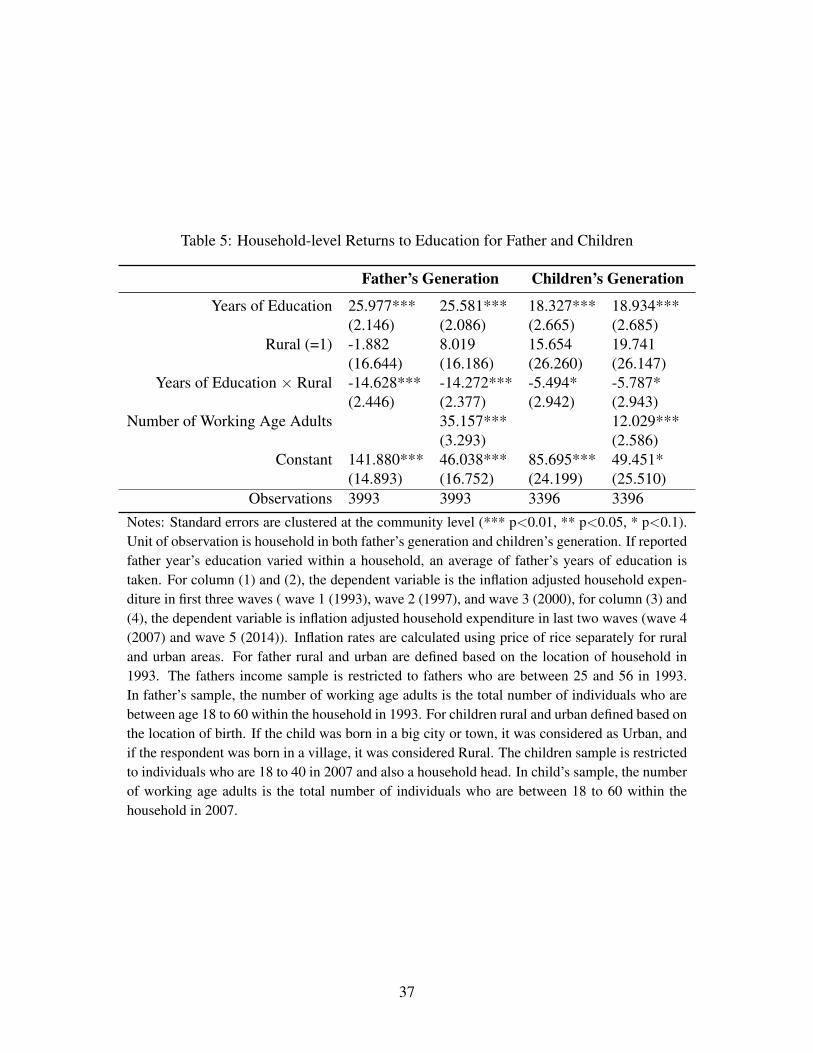
Table 5: Household-level Returns to Education for Father and Children

Father’s Generation Children’s Generation

Years of Education 25.977*** 25.581*** 18.327*** 18.934***(2.146) (2.086) (2.665) (2.685)

Rural (=1) -1.882 8.019 15.654 19.741(16.644) (16.186) (26.260) (26.147)

Years of Education × Rural -14.628*** -14.272*** -5.494* -5.787*(2.446) (2.377) (2.942) (2.943)

Number of Working Age Adults 35.157*** 12.029***(3.293) (2.586)

Constant 141.880*** 46.038*** 85.695*** 49.451*(14.893) (16.752) (24.199) (25.510)

Observations 3993 3993 3396 3396Notes: Standard errors are clustered at the community level (*** p<0.01, ** p<0.05, * p<0.1).Unit of observation is household in both father’s generation and children’s generation. If reportedfather year’s education varied within a household, an average of father’s years of education istaken. For column (1) and (2), the dependent variable is the inflation adjusted household expen-diture in first three waves ( wave 1 (1993), wave 2 (1997), and wave 3 (2000), for column (3) and(4), the dependent variable is inflation adjusted household expenditure in last two waves (wave 4(2007) and wave 5 (2014)). Inflation rates are calculated using price of rice separately for ruraland urban areas. For father rural and urban are defined based on the location of household in1993. The fathers income sample is restricted to fathers who are between 25 and 56 in 1993.In father’s sample, the number of working age adults is the total number of individuals who arebetween age 18 to 60 within the household in 1993. For children rural and urban defined based onthe location of birth. If the child was born in a big city or town, it was considered as Urban, andif the respondent was born in a village, it was considered Rural. The children sample is restrictedto individuals who are 18 to 40 in 2007 and also a household head. In child’s sample, the numberof working age adults is the total number of individuals who are between 18 to 60 within thehousehold in 2007.

37

Table 6A: Effects of Peers on Financial Investment on Childrens Education

Rural (R) Urban (U) R–U Rural (R) Urban (U) R–U

Father Edu 0.048*** 0.109*** -0.061*** 0.049*** 0.112*** -0.063***(0.006) (0.010) (0.011) (0.006) (0.010) (0.012)

Peer Edu 0.026 0.141*** -0.115** 0.026 0.135*** -0.110**(0.023) (0.046) (0.050) (0.022) (0.045) (0.050)

Number of School Age Children -0.022 -0.081***(0.019) (0.026)

Constant 0.059 -0.819* -0.043 -0.812*(0.206) (0.448) (0.203) (0.444)

Includes Ability No No No Yes Yes YesObservations 9463 8311 17774 9463 8311 17774Notes: Standard errors are clustered at the community level (*** p<0.01, ** p<0.05, * p<0.1). The dependent variable iseducational expenditure adjusting for inflation. Inflation rates are calculated using price of rice separately for rural and urbanareas. A peer is someone who was born in the respondents district within ±3 years of respondents birth. Rural and Urban aredefined based on location of birth. If the respondent was born in a big city or town, it was considered as Urban, and if therespondent was born in a village, it was considered Rural. Cognitive ability index is expressed in percentile; it is constructedtaking the first principal component of Raven Test and two memory memory tests net of age and age square. Ability controlsinclude cognitive ability index and its square.

Table 6B: Peer Effect and Intergenerational Educational Mobility

Rural (R) Urban (U) R–U Rural (R) Urban (U) R–U

Father Edu 0.325*** 0.528*** -0.203** 0.307*** 0.471*** -0.164(0.064) (0.089) (0.101) (0.063) (0.087) (0.100)

Father Edu Sq 0.013*** 0.012*** 0.001 0.013*** 0.012*** 0.001(0.002) (0.002) (0.003) (0.002) (0.002) (0.003)

Father Edu × Peer -0.020*** -0.037*** 0.017 -0.022*** -0.034*** 0.012(0.008) (0.010) (0.011) (0.007) (0.009) (0.011)

Peer Edu 0.840*** 0.753*** 0.088 0.579*** 0.650*** -0.071(0.170) (0.233) (0.285) (0.150) (0.217) (0.262)

Peer Edu Sq 0.003 0.014 -0.01 0.016* 0.014 0.002(0.010) (0.013) (0.016) (0.009) (0.012) (0.015)

Constant -0.223 -0.684 0.461 -0.253 -0.76 0.298(0.755) (1.140) (1.372) (0.632) (1.071) (1.241)

Includes Ability No No No Yes Yes YesObservations 9907 5087 14994 9907 5087 14994Notes: Standard errors are clustered at the community level (*** p<0.01, ** p<0.05, * p<0.1). A peer issomeone who was born in the respondents district within ±3 years of respondents birth. Rural and Urbanare defined based on location of birth. If the respondent was born in a big city or town, it was consideredas Urban, and if the respondent was born in a village, it was considered Rural. Cognitive ability index isexpressed in percentile; it is constructed taking the first principal component of Raven Test and two memorymemory tests net of age and age square. Ability controls include cognitive ability index and its square.

38

Table 7A: Effects of Role Model on Financial Investment on Childrens Education

Rural (R) Urban (U) R–U Rural (R) Urban (U) R–UFather Edu 0.052*** 0.124*** -0.072*** 0.053*** 0.126*** -0.073***

(0.006) (0.012) (0.013) (0.006) (0.012) (0.013)Role Model Edu -0.009 -0.044*** 0.036* -0.009 -0.045*** 0.036*

(0.014) (0.015) (0.021) (0.013) (0.015) (0.020)Number of School Age Children -0.021 -0.055*

(0.019) (0.030)Constant 0.365*** 0.868*** 0.255** 0.761***

(0.104) (0.188) (0.112) (0.205)Includes Ability No No No Yes Yes YesObservations 8485 7281 15766 8485 7281 15766Notes: Standard errors are clustered at the community level (*** p<0.01, ** p<0.05, * p<0.1). The dependent variable iseducational expenditure adjusting for inflation. Inflation rates are calculated using price of rice separately for rural and urbanareas. A peer is someone who was born in the respondents district within ±3 years of respondents birth. Rural and Urban aredefined based on location of birth. If the respondent was born in a big city or town, it was considered as Urban, and if therespondent was born in a village, it was considered Rural. Cognitive ability index is expressed in percentile; it is constructedtaking the first principal component of Raven Test and two memory memory tests net of age and age square. Ability controlsinclude cognitive ability index and its square.

Table 7B: Role Models and Intergenerational Educational Mobility

Rural (R) Urban (U) R–U Rural (R) Urban (U) R–UFather Edu 0.238*** 0.384*** -0.146** 0.200*** 0.351*** -0.151**

(0.039) (0.056) (0.063) (0.037) (0.053) (0.060)Father Edu Sq 0.015*** 0.011*** 0.005 0.016*** 0.011*** 0.005*

(0.002) (0.002) (0.003) (0.002) (0.002) (0.003)Father Edu × Role Model -0.011** -0.014*** 0.003 -0.010** -0.014*** 0.004

(0.004) (0.004) (0.006) (0.004) (0.004) (0.006)Role Model Edu 0.229*** 0.103 0.126 0.189*** 0.104 0.085

(0.061) (0.118) (0.124) (0.057) (0.112) (0.118)Role Model Edu Sq -0.004 0.002 -0.006 -0.003 0.002 -0.004

(0.004) (0.005) (0.006) (0.003) (0.005) (0.006)Constant 5.988*** 6.389*** -0.401 4.722*** 5.406*** -0.6836

(0.285) (0.682) (0.676) (0.272) (0.683) (0 .671)Includes Ability No No No Yes Yes YesObservations 8292 4111 12403 8292 4111 12403Notes: Standard errors are clustered at the community level (*** p<0.01, ** p<0.05, * p<0.1). A rolemodel is someone who was born in the respondent’s district but is within ±3 of respondent’s father age andbelongs to top 50 percent education level within that age group of that district. Rural and Urban are definedbased on location of birth. If the respondent was born in a big city or town, it was considered as Urban,and if the respondent was born in a village, it was considered Rural. Cognitive ability index is expressedin percentile; it is constructed taking the first principal component of Raven Test and two memory memorytests net of age and age square. Ability controls include cognitive ability index and its square.

39

Online Data Appendix: Not for Publication

The Indonesian Family Life Survey (IFLS) is an ongoing longitudinal survey.

So far five waves have been fielded. The first wave was fielded in 1993, and

the second, third, fourth and fifth waves were fielded in 1997, 2000, 2007

and 2014, respectively. At the time of the first wave, 7224 households were

interviewed and it represented 83 % of the national population of Indone-

sia covering 13 out of the 27 provinces (Frankenberg et al., 1995). In the

subsequent waves, the sample size grew because others joined the sampled

households either through marriage and births. An appealing feature of the

IFLS is its low-attrition rate (Strauss et al., 2016).

Below we provide detailed discussion and rationale on how we have ob-

tained different variables from the IFLS data:

Children Sample: As noted in data section, our primary mobility sam-

ple is based on children who are 18 to 40 years old in 2014 (wave 5). We

restrict the sample to 18 to 40 years old of the fifth wave for two reasons.

First, these individuals were in school at some point during 1990s and 2000s.

Therefore, we can use the previous waves to estimate the effects on school-

ing investment. Secondly, only in the fifth wave, the IFLS started to collect

Raven Test scores a measure of “fluid intelligence” for all adults. Since we

include cognitive ability in much of our analysis, we have chosen to use the

fifth wave for our children sample.

Child Years of Education: In order to obtain the child years of ed-

ucation, we use two sources of data in the fifth wave of the IFLS: book 3A

and roster. Book 3A has education information for anyone who is 15 years

and older. If the 18 to 40-year-old household member do not have education

reported in book 3A, we use the education reported in roster.

1

Father’s Years of Education: We use three sources to calculate fa-

ther’s years of education. Below we discuss each source:

Household roster: As noted above, the IFLS household roster reports

education information of the household member. Moreover, the roster data

also provides household member ID of father and mother of each child listed

in the roster. Starting with the latest (fifth) wave, we check if the father has

co-resided with children at any wave. If the father has co-resided with the

children during the any wave, we obtain the education information from the

latest wave in which the father has co-resided with the children.

Non-resident parents module: For any household member who is 15 years

and older, the IFLS asks about parental education if the parents are not

residing in the same household. If the child did not co-reside with the father

in any of the survey waves, we use this module to obtain father’s years

of education. Using the panel ID, we identify the latest wave in which the

children have reported parental education of non-resident parents and extract

that education information.

Mothers marriage module: Ideally, we should be able to find education

information all fathers using the above two sources. But in some cases, the

fathers’ education is missing because of non-response or the reported value

exceed any meaningful years of schooling value. The IFLS asks all married

women about their husband’s years of education if the husband is not residing

in the household. If we unable to find father’s years of education using above

two sources, we identify if the mother has co-resided with the child in any

of the waves. If the mother co-resided with the child, we then use mother’s

marriage module to obtain fathers’ schooling information.

Using all three sources, we are able to collect fathers’ education informa-

tion for almost 90 percent of the sample.

2

Children’s Birth Location: For any household member who are 15 or

older, the IFLS has information about the location types of birth: village,

small town, or a big city. If the respondents were born in a village, we define

the birth location as rural and otherwise, urban. The IFLS collects this

information in all waves. For any respondent, we use the birth location in

the latest wave in which the respondent reported his/her birth location type.

Child Cognitive Ability: We use the Raven test scores and two mem-

ory tests to construct the cognitive ability index. An advantage of these

measures is that they do not require any knowledge of numeracy or literacy

to do well in the tests. To arrive at the index, we first take the first principal

component of the raven test scores and two memory tests. Then we regress

that on age and age square. A critical issue is that cognition outcomes are

positively correlated with age because of the Flynn effect. We, therefore, use

residual of the regression as the cognitive ability index.

Education Expenses: The IFLS has separate education modules for

children (age below 15) and adult (age equal to or above 15). The expense

data includes all types of school-related expenses. We aggregate the expenses

Using the Panel ID, we match individuals of our children sample (18 to 40

years old in wave 5) with their education expense data in the previous waves.

The expenses are then adjusted for inflation taking 1993 as the base year; we

obtain the yearly inflation of Indonesia from the World Bank web site.

In the investment sample, we also control for number of school age of

children. To calculate the number of school children in wave, we first obtain

the fathers’ ID from the roster. We then calculate how many other individuals

in the education sample also listed as the same ID as the father. That number

provides us with the number of school age children. Finally, in the investment

sample, we also include whether the household is located in urban area or

3

rural area. In each wave, the household location information is available in

book K. We match the household ID with the location information.

Permanent income: We use the household expenditures as a proxy for

income, since income data often suffer from more measurement error than

household expenditure. For the fathers’ generation, we use the average of

household consumption expenditure of the first three waves, and the chil-

dren’s generation, we the average of household consumption expenditure of

the last two waves. Below we discuss in more details how we calculate the

permanent income:

Fathers’ generation permanent income:

For each of the first three waves, we first separately calculate the house-

hold expenditure. For each household member, the IFLS provides his/her

relationship to household head. We identify the households in which the in-

dividuals of our children sample (18 to 40 years old in 2014) were listed as

children or grandchildren in the any of the first three waves. We consider

both children and grandchildren because these children may grow up in an

extended family where the grandfather is household head. Using the house-

hold tracking id, we then merge the identified households with their total

expenditures. We adjust for inflation by using yearly inflation data from the

World bank web site taking 1993 as the base year. After this we merge the

sample with fathers’ age information. We restrict the sample to fathers who

are age 25 to 56 in 1993.

Children’s Generation Permanent Income:

For each of the last two waves, we first calculate the household expendi-

ture. Since we want to focus on children who are 25 to 56 years old in 2007,

we extend the original children sample to this age group. We then identify

children who are household heads in 2007. We wanted to make sure the chil-

4

dren are household heads because if the children are living with parents, we

may falsely attribute the permanent income of children to parents. Then we

merge the household expenditure of the fourth wave (2007) with the house-

hold expenditure of the fifth wave (2014) using the household tracking ID.

We adjust inflation taking 1993 as the base year.

Role model data: The role model in our study are individuals who

were born in the same district as the child and belong to the top 50 percent

of education distribution of fathers’ reference age group. To calculate the

role model education, we first needed to obtain fathers’ age. We check if the

father has co-resided with children in any of waves. If we can find the father,

we obtain the age from the household roster and convert that value to what

his age would be in 2014. For the non-resident father, we obtain the age from

the non-resident module. The IFLS asks age at death and year of death, if

the father is not alive. Using this information, we calculate what would have

been fathers’ age in 2014. We then obtain the birth district information

of the children. Separately, next we use the roster data of each wave to

obtain years of education and age of all individuals who are older than 22

at the time of the survey. We choose older than 22 because by age 22 the

individuals would have completed their education. Then we convert the age

of these individuals to the value it would be in 2014. Using the birth district

information, we obtain the birth district of all the individuals in the roster.

For any given age, we calculate the average of years of education of the top

50 percent achievers within the ±3 (±5 for robustness check) age group of

a district. We then merge the district ID information and age information

with the birth district ID and father age information of the data above.

Peer Data: We select individuals who are within ±3 (±5 for robustness

check) of the age group of our children sample and born in the same district

5

as the children. First, we create a data where we include individuals who

are 15 to 43 years old. We then obtain years of education and birth district

information for these individuals. After that, we take the average years of

education for ±3 (±5 for robustness check) of the age group for each district.

We then restrict that sample to 18 to 40 years old and merge the sample to

the original

References

Frankenberg, Elizabeth, Lynn A Karoly, Paul Gertler, Sulistinah

Achmad, IGN Agung, Sri Harijati Hatmadji, and Paramita Sud-

harto, “The 1993 Indonesian family life survey: Overview and field re-

port,” 1995.

Strauss, John, Firman Witoelar, and Bondan Sikoki, The fifth wave

of the Indonesia family life survey: overview and field report, Vol. 1, RAND

Santa Monica, CA, 2016.

6

Online Appendix: Not for Publication

Table A1: Education and Cognition Interaction

Rural UrbanFather Edu 0.333*** 0.226*** 0.408*** 0.278**

(0.021) (0.071) (0.027) (0.121)Ability Index 0.524*** 0.702*** 0.333*** 0.420*

(0.055) (0.109) (0.066) (0.225)Ability Index Sq -0.029*** -0.046*** -0.007 -0.015

(0.004) (0.010) (0.006) (0.022)Father Edu × Ability Index 0.004 -0.044 -0.002 -0.003

(0.003) (0.030) (0.004) (0.055)Father Edu Sq 0.013** 0.011

(0.006) (0.007)Father Edu × Ability Index Sq 0.005* 0.000

(0.003) (0.005)Father Edu Sq × Ability Index 0.002 -0.001

(0.002) (0.003)Father Edu Sq × Ability Index Sq -0.000 0.000

(0.000) (0.000)Constant 5.432*** 5.510*** 5.673*** 5.889***

(0.201) (0.282) (0.237) (0.490)Observations 10239 10239 5238 5238Notes: Standard errors are clustered at the community level (*** p<0.01, ** p<0.05, *p<0.1). Rural and Urban are defined based on location of birth. If the respondent wasborn in a big city or town, it was considered as Urban, and if the respondent was bornin a village, it was considered Rural. Cognitive ability index is expressed in percentile;it is constructed taking the first principal component of Raven Test and two memorymemory tests net of age and age square.

1

Table A2: Effects of Peers and Role Models on Financial Investment on Childrens Education

Father Edu 0.115*** 0.115*** 0.117***(0.012) (0.012) (0.012)

Peer Edu 0.159*** 0.161*** 0.155***(0.051) (0.051) (0.050)

Role Model Edu -0.066*** -0.067*** -0.066***(0.017) (0.017) (0.017)

HH Rural (=1) 0.584 0.570 0.564(0.486) (0.486) (0.479)

Father Edu × Rural -0.063*** -0.063*** -0.063***(0.013) (0.013) (0.013)

Peer Edu × Rural -0.133** -0.133** -0.128**(0.056) (0.055) (0.055)

Role Model Edu × Rural 0.053** 0.053** 0.052**(0.022) (0.022) (0.022)

Number of School Age Children -0.041** -0.040**(0.017) (0.017)

Ability Index 0.016(0.026)

Ability Index Sq 0.002(0.003)

Constant -0.416 -0.359 -0.484(0.448) (0.450) (0.451)

Observations 15766 15766 15766Notes: Standard errors are clustered at the community level (*** p<0.01,** p<0.05, * p<0.1). The dependent variable is educational expenditureadjusting for inflation. Inflation rates are calculated using price of rice sep-arately for rural and urban areas. The peer and role model measures in PanelC are only based on district level. A peer is someone who was born in therespondents district within ±3 years of respondents birth. A role model issomeone who was born in the respondent’s district but is within ±3 of re-spondent’s father age and belongs to top 50 percent education level withinthat age group of that district. All regressions include wave fixed effects.Rural and urban are defined based on location of household at the time ofsurvey. Cognitive ability index is expressed in percentile; it is constructedtaking the first principal component of Raven Test and two memory memorytests net of age and age square.

2

Table A3: Effects of Peers on Financial Investment on Childrens Education (Robustness): Alter-native Definition of Peer Group: ±5 Years Age Band

Rural (R) Urban (U) R–U Rural (R) Urban (U) R–U

Father Edu 0.049*** 0.109*** -0.061*** 0.050*** 0.112*** -0.062***(0.006) (0.010) (0.011) (0.006) (0.010) (0.011)

Peer Edu 0.024 0.158*** -0.134*** 0.023 0.153*** -0.130**(0.023) (0.046) (0.051) (0.022) (0.046) (0.051)

Number of School Age Children -0.021 -0.082***(0.026) (0.038)

Constant 0.082 -0.982** -0.021 -0.979**(0.211) (0.445) (0.204) (0.445)

Includes Ability No No No Yes Yes YesObservations 9463 8311 17774 9463 8311 17774Notes: Standard errors are clustered at the community level (*** p<0.01, ** p<0.05, * p<0.1). The dependentvariable is educational expenditure adjusting for inflation. Inflation rates are calculated using price of rice separatelyfor rural and urban areas. A peer is someone who was born in the respondents district within ±5 years of respondentsbirth. Rural and Urban are defined based on location of birth. If the respondent was born in a big city or town, it wasconsidered as Urban, and if the respondent was born in a village, it was considered Rural. Cognitive ability index isexpressed in percentile; it is constructed taking the first principal component of Raven Test and two memory memorytests net of age and age square. Ability controls include cognitive ability index and its square.

3

Table A4: Peer Effect and Intergenerational Educational Mobility (Robustness): Alternative Defi-nition of Peer Group: ±5 Years Age Band

Rural (R) Urban (U) R–U Rural (R) Urban (U) R–UFather Edu 0.309*** 0.546*** -0.236** 0.295*** 0.488*** -0.194*

(0.075) (0.098) (0.111) (0.073) (0.096) (0.111)Father Edu Sq 0.013*** 0.012*** 0.001 0.013*** 0.012*** 0.001

(0.002) (0.002) (0.003) (0.002) (0.002) (0.003)Father Edu × Peer -0.018** -0.039*** 0.021* -0.020** -0.035*** 0.015

(0.009) (0.011) (0.012) (0.009) (0.010) (0.012)Peer Edu 1.003*** 0.621** 0.382 0.723*** 0.507* 0.216

(0.206) (0.298) (0.340) (0.187) (0.278) (0.315)Peer Edu Sq -0.006 0.02 -0.026 0.008 0.022 -0.013

(0.013) (0.016) (0.019) (0.012) (0.015) (0.018)Constant -0.958 -0.039 -0.919 -0.918 -0.102 -0.816

(0.864) (1.424) (1.604) (0.741) (1.340) (1.462)Includes Ability No No No Yes Yes YesObservations 9907 5087 14994 9907 5087 14994Notes: Standard errors are clustered at the community level (*** p<0.01, ** p<0.05, * p<0.1).A peer is someone who was born in the respondents district within ±5 years of respondents birth.Rural and Urban are defined based on location of birth. If the respondent was born in a big city ortown, it was considered as Urban, and if the respondent was born in a village, it was consideredRural. Cognitive ability index is expressed in percentile; it is constructed taking the first principalcomponent of Raven Test and two memory memory tests net of age and age square. Abilitycontrols include cognitive ability index and its square.

4

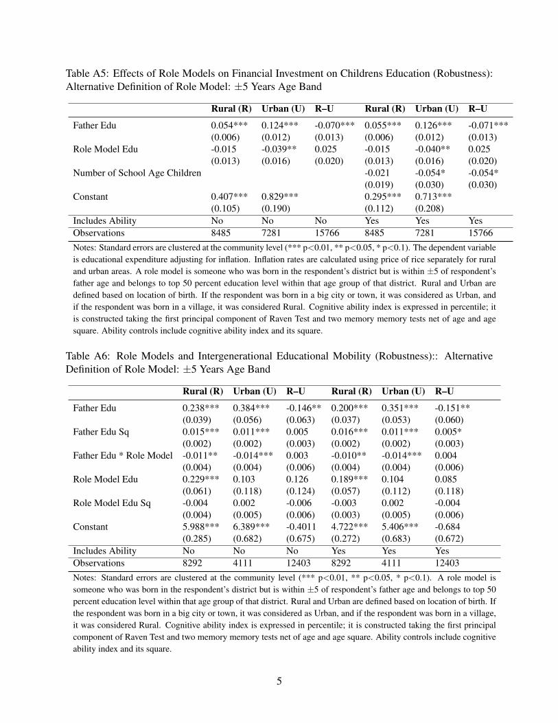
Table A5: Effects of Role Models on Financial Investment on Childrens Education (Robustness):Alternative Definition of Role Model: ±5 Years Age Band

Rural (R) Urban (U) R–U Rural (R) Urban (U) R–U

Father Edu 0.054*** 0.124*** -0.070*** 0.055*** 0.126*** -0.071***(0.006) (0.012) (0.013) (0.006) (0.012) (0.013)

Role Model Edu -0.015 -0.039** 0.025 -0.015 -0.040** 0.025(0.013) (0.016) (0.020) (0.013) (0.016) (0.020)

Number of School Age Children -0.021 -0.054* -0.054*(0.019) (0.030) (0.030)

Constant 0.407*** 0.829*** 0.295*** 0.713***(0.105) (0.190) (0.112) (0.208)

Includes Ability No No No Yes Yes YesObservations 8485 7281 15766 8485 7281 15766Notes: Standard errors are clustered at the community level (*** p<0.01, ** p<0.05, * p<0.1). The dependent variableis educational expenditure adjusting for inflation. Inflation rates are calculated using price of rice separately for ruraland urban areas. A role model is someone who was born in the respondent’s district but is within ±5 of respondent’sfather age and belongs to top 50 percent education level within that age group of that district. Rural and Urban aredefined based on location of birth. If the respondent was born in a big city or town, it was considered as Urban, andif the respondent was born in a village, it was considered Rural. Cognitive ability index is expressed in percentile; itis constructed taking the first principal component of Raven Test and two memory memory tests net of age and agesquare. Ability controls include cognitive ability index and its square.

Table A6: Role Models and Intergenerational Educational Mobility (Robustness):: AlternativeDefinition of Role Model: ±5 Years Age Band

Rural (R) Urban (U) R–U Rural (R) Urban (U) R–U

Father Edu 0.238*** 0.384*** -0.146** 0.200*** 0.351*** -0.151**(0.039) (0.056) (0.063) (0.037) (0.053) (0.060)

Father Edu Sq 0.015*** 0.011*** 0.005 0.016*** 0.011*** 0.005*(0.002) (0.002) (0.003) (0.002) (0.002) (0.003)

Father Edu * Role Model -0.011** -0.014*** 0.003 -0.010** -0.014*** 0.004(0.004) (0.004) (0.006) (0.004) (0.004) (0.006)

Role Model Edu 0.229*** 0.103 0.126 0.189*** 0.104 0.085(0.061) (0.118) (0.124) (0.057) (0.112) (0.118)

Role Model Edu Sq -0.004 0.002 -0.006 -0.003 0.002 -0.004(0.004) (0.005) (0.006) (0.003) (0.005) (0.006)

Constant 5.988*** 6.389*** -0.4011 4.722*** 5.406*** -0.684(0.285) (0.682) (0.675) (0.272) (0.683) (0.672)

Includes Ability No No No Yes Yes YesObservations 8292 4111 12403 8292 4111 12403Notes: Standard errors are clustered at the community level (*** p<0.01, ** p<0.05, * p<0.1). A role model issomeone who was born in the respondent’s district but is within ±5 of respondent’s father age and belongs to top 50percent education level within that age group of that district. Rural and Urban are defined based on location of birth. Ifthe respondent was born in a big city or town, it was considered as Urban, and if the respondent was born in a village,it was considered Rural. Cognitive ability index is expressed in percentile; it is constructed taking the first principalcomponent of Raven Test and two memory memory tests net of age and age square. Ability controls include cognitiveability index and its square.

5