The Role of “Volume Dispersion” in Explaining the

Price Change-Volume Relation at the Index Level *

Eric C. Chang School of Business

The University of Hong Kong Pokfulam Road, Hong Kong ecchang@business.hku.hk

(852) 2857-8347

Joseph W. Cheng The Chinese University of Hong Kong

Shatin, New Territories Hong Kong

jcheng@cuhk.edu.hk (852) 2609-7904

and

Ajay Khorana

DuPree College of Management Georgia Institute of Technology

Atlanta, GA 30332-0520 ajay.khorana@mgt.gatech.edu

(404) 894-5110

January 2004 __________________ * We would like to thank Paula Tkac and seminar participants at the 2001 Financial Management Association Meetings for helpful comments and suggestions.

The Role of “Volume Dispersion” in Explaining the Price Change-Volume Relation at the Index Level

Abstract In this paper, we examine the dynamics of the price change-trading volume relation at the aggregate market/index level. We introduce the use of a novel “volume dispersion” measure designed to proxy for the variability in firm-specific information flows across securities that comprise the market. Our results suggest that the price change-volume relation can be strengthened by the introduction of this measure. We also offer evidence of a positive relation between market volatility and trading volume and a negative relation between market volatility and volume dispersion. Furthermore, we demonstrate that lagged values of market level trading volume and volume dispersion can predict the next day’s index level volatility. Our findings remain robust when the implied volatility of the S&P 100 index options is used in the analysis. This suggests that index option traders need to pay close attention to both aggregate market level trading volume and volume dispersion to better capture the dynamics of daily market volatility.

1

I. Introduction

Considerable research attention has been given to the relation between security price changes and the

trading volume accompanying the underlying price change. Some practitioners argue that volume is a useful

indicator to facilitate their security selection and/or market timing decisions.1 Fundamentally, the greater the

difference of opinions or differential interpretations of public signals among traders, the greater the expected

level of speculative trading [see for example Harris and Raviv (1993) and Kandel and Pearson (1995)]. Blume,

Easley, and O’Hara (1994) in particular have developed a model which shows that volume can provide valuable

insight into the quality of information impounded in the prices of individual stocks. To the extent that trading is

a mechanism for the dissemination of information in security prices, it is important to pay closer attention to the

price change-volume relation.

In recent years, financial markets have also witnessed a surge of interest in index-based financial products.

A number of new financial instruments, such as index futures, index options, index depository receipts (e.g.

Spiders) and exchange traded funds (ETFs), have been introduced in developed financial markets. 2 The

popularity of these new instruments calls for a better understanding of the dynamics of the price change-volume

relation at the aggregate market/index level.

Previous studies have examined the price change-volume relation either at the level of individual stocks

(Epps (1975); Morse (1980); Harris (1986); Conrad, Hameed and Niden (1992); Stickel and Verrecchia (1994))

or at the aggregate stock market level (Granger and Morgenstein (1963); Ying (1966); Jain and Joh (1988);

Gallant, Rossi and Tauchen (1992); Campbell, Grossman and Wang (1993)).3 However, these studies do not

explicitly recognize the differences in the relation across the two levels, i.e. the individual stock versus the

aggregate market index level.4

1 Conrad, Hameed, and Niden (1994) and Gervais, Kaniel, and Mingelgrin (2001) demonstrate empirically that share turnover can predict future returns of individual stocks. 2 This trend can be partly explained by Gordon and Pennacchi (1993), who suggest that instead of trading individual securities, market participants with superior market-wide information (e.g. a better forecast of interest rates) will prefer to trade a basket of stocks due to lower transaction and adverse selection costs. 3 See also Karpoff (1987) for a survey of the literature regarding earlier studies on the price change-volume relation. 4 Gallant, Rossi and Tauchen (1992) and Campbell, Grossman and Wang (1993) suggest that aggregate market returns tend to reverse themselves on high-volume days while Stickel and Verrecchia (1994) demonstrate that an individual security’s

2

The objectives of this paper are empirically oriented and are aimed at broadening our understanding of the

price change and volume relation. We pay close attention to the explicit differences between the price change-

volume relation at the individual security level and at the aggregate market index level. We argue that when

examining the price change-volume relation at the market level, it is important to explicitly distinguish between

the role played by aggregate market level trading volume and the variation in trading volume due to firm-

specific information across individual securities that comprise the market. We propose an alternative regression

model which is more appropriate for investigating the fundamental relation between the price change of a

market index and the index trading volume accompanying the price change. Since market size may have a non-

trivial impact on the price change-volume relation,5 we examine the relation using data from the U.S. and

Japanese equity markets.

Our empirical work supplements existing price change-volume studies along three major dimensions. First,

we examine whether the price change-volume relation observed for individual stocks also holds for the market

index. Second, we examine the underlying relation between stock index return volatility (as measured by the

absolute value of the price change) and trading volume at the aggregate market level. Finally, we propose a new

measure to proxy for the dispersion in the rate of information flow at the individual security level, and examine

its usefulness in explaining the price change-volume/volatility-volume relation at the aggregate market level.

The motivation for using the new information flow (i.e. volume) dispersion measure in the index/portfolio

level price change-volume tests is straightforward. In most cases trading by market participants is triggered by

the arrival of either macroeconomic or firm-specific information. Trading caused by macroeconomic

information shocks will tend to cause a similar directional movement in stock prices. On the other hand, trading

caused by the arrival of firm-specific information, whether public or private in nature, will lead to a greater

dispersion in both the magnitude and the direction of movements in the prices of the underlying assets. Given

returns are more sustainable on high-volume days. However, these studies do not offer any explanation to reconcile the contrasting findings for the aggregate market versus individual securities. 5 Tauchen and Pitts (1983) show that the strength of the correlation between volume and price change is an increasing function of the number of investors in the market. Harris (1986) demonstrates that the price change-volume relation is stronger in markets with more volatile information flows.

3

that both of these effects may play a crucial role in determining the variability in trading at the aggregate market

level, we argue that it is imperative to take them into consideration in the analysis of the market index level

price change-volume relation. Our “volume (turnover) dispersion” measure utilizes trading volume information

at the individual security level and is designed to partially control for the variability in the dissemination of

public or private firm-specific information across securities that comprise the market. Specifically, by utilizing

market model regressions of turnover,6 we proxy for the latter by the absolute value of the cross-sectional

deviations in abnormal trading volume (volume turnover), i.e. ADT.

Using return and volume data for the U.S. (Japan) over the period from 1963 (1975) to 1998 (1996) at the

individual security level, we reconfirm the V-shaped relation suggested by previous researchers. In other words,

we document a positive price change-volume relation in up-markets and a negative relation in down-markets.

We then examine the price change-volume relation at the aggregate market level. However, the results indicate

that the V-shaped price change-volume relation found at the individual security level does not always hold at the

level of the aggregate market. On the other hand, we show that the expected directional relations can be re-

established by the inclusion of the omitted volume dispersion variable.

We demonstrate that the price change-volume relation found at the individual security level can indeed be

strengthened at the aggregate market level by the introduction of the volume (volume turnover) dispersion (i.e.

ADT) measure. In fact, the introduction of the ADT measure significantly increases the explanatory power of the

regression specifications. The regression models that include the turnover dispersion measure have adjusted R2

of 51%-53% (44%-47%) for the U.S. (Japan) compared to adjusted R2 of 47%-50% (40%-42%) for the models

that exclude this measure. Furthermore, the coefficient on the turnover dispersion measure is negative in the up-

markets and positive in the down-markets. This suggests that, ceteris paribus, large positive or negative market

returns are associated with lower levels of dispersion in abnormal volume at the firm level.

In subsequent tests, we also examine the contemporaneous relation between the absolute value of the price

change (a measure of price variability, e.g., Grammatikos and Saunders (1986)), market level trading volume

6 The use of the market model regressions of turnover was initiated by Tkac (1999), and Lo and Wang (2000).

4

turnover, and the turnover dispersion measure. The relation between price variability and trading volume has

received considerable attention in finance. Theoretical models proposed to explain the correlation between

volatility and trading volume include models of asymmetric information (Kyle (1985); Admati and Pfleiderer

(1988); Holden and Subrahmanyam (1992)), disagreement of opinion (Varian (1985); Harris and Raviv (1993);

Wang (1993)), and mixture of distributions (Epps and Epps (1976); Tauchen and Pitts (1983); Harris (1986)). A

positive relation between price variability, as measured by the absolute value of price change, and trading

volume has also been documented in earlier studies.7 Using Nasdaq securities, Jones, Kaul, and Lipson (1994b)

report that the volatility-volume (turnover) relation no longer holds when the influence of the number of trades

is accounted for in the analysis. However, using a sample consisting of both NYSE and Nasdaq securities, Chan

and Fong (2000) re-establish the positive relation between volume and volatility.8 We conjecture, however, that

in addition to a positive relation between market volatility and trading volume, a negative relation between

market volatility and turnover dispersion should also be observed. Moreover, the inclusion of the turnover

dispersion measure in the volatility regressions should add significant explanatory power to the model. Our

empirical work confirms both predictions. Furthermore, we demonstrate that lagged values of market level

trading volume and turnover dispersion can predict the next day’s index-level volatility. Our findings remain

robust when the implied volatility of the S&P 100 index options is used in the analysis. This suggests that index

option traders need to pay close attention to both aggregate market level trading volume and turnover dispersion

to better capture the dynamics of daily market volatility. Overall, our results suggest that firm level volume data

plays an important role in understanding the market level return-volume behavior.

The remainder of the paper is organized as follows. Section II elaborates on the motivation and construction

of the turnover dispersion measure. Section III describes the data and methodology used for the analysis.

7 For example, see Morgan (1976); Tauchen and Pitts (1983); Wood, McInish and Ord (1985); Harris (1986); Karpoff (1987); and Jain and Joh (1988). Recent studies (Schwert (1989); Lamoureux and Lastrapes (1990); Gallant, Rossi, and Tauchen (1992); Daigler and Wiley (1999)) provide additional evidence for the volume-volatility relation. Various data frequencies (transaction, hourly, daily, weekly and monthly data) have been employed to examine the behavior of aggregate market index as well as individual securities for the stock and the futures market. The positive volatility-volume relation remains robust. 8 Using bivariate threshold theory to model the joint distribution of absolute returns and trading volume, Qi (2001) provides evidence of a positive relation between the two variables for a sample of six emerging markets. However, this

5

Section IV contains the results and Section V concludes.

II. The Trading Volume Dispersion Measure

A. Motivation

Several empirical studies have documented a positive correlation between a security’s price change and the

accompanying trading volume and between the absolute value of price change and trading volume in various

equity markets.9 Epps (1975), Karpoff (1987), and Jennings, Starks and Fellingham (1981) have demonstrated

that large price increases (and decreases) are accompanied by higher levels of trading volume. Furthermore,

ceteris paribus, price declines are usually accompanied by a relatively small trading volume, while price

increases are associated with a large trading volume. These and other studies have demonstrated that the price

change-volume relation is asymmetric between up-markets and down-markets. As depicted in Diagram 1, this

asymmetry produces a V-shaped pattern.

The asymmetric relation can also be captured by the following two time-series regression specifications:

0∆Pfor , it10 >++=∆ ititupup

it VaaP ε (1)

0∆Pfor , it10 <++=∆ ititdowndown

it VaaP ε (2)

where itP∆ denotes the price change of security i on date t, Vit is the trading volume (or turnover rate) of

relation is significantly weakened during periods of extreme price movements. 9 Wang (1994) offers a theoretical model that also suggests that trading volume is positively correlated with the absolute

Volume

Diagram 1

∆ P < 0 ∆ P > 0

6

security i on date t, and εit is an error term10. Existing evidence suggests that a1up > 0, a1

down < 0 and a1up < - a1

down.

Moreover, empirical evidence also supports the presence of a positive γ1 coefficient in the following regression:

ititit VP ηγγ ++=∆ 10|| (3)

A common message that can be construed from equations (1), (2), and (3) is that, for individual securities, the

time-series variation in trading volume helps explain the variability in price changes over time.

In Figure 1, using daily return (in percentage terms) and turnover data of all US (Japan) individual securities

available on the CRSP (PACAP) database during the period 1963-1998 (1975-1996), we provide a graphical

illustration of the above relationship. Specifically, the daily return observations of each individual firm are

partitioned into turnover quintiles according to the size of the firm’s daily turnover during the sample period,

with quintile T1 (T5) containing observations with the lowest (highest) turnover rate. The return observations

within each of the five turnover quintiles are further partitioned into an up-market sample (positive daily return)

and a down-market sample (negative daily return). The process is repeated for all valid sample firms in the two

databases11. For each of the 10 turnover groups, an equally-weighted average return is computed. The overall

return average for all individual firms in the US (Japan) sample within each of the 10 turnover groups is

displayed in Panel A (B) of Figure 1. The figure shows that, for the individual firm sample, average daily return

increases (decreases) monotonically with turnover in the up-market (down-market) for both the US and Japan.

This finding is, therefore, consistent with the hypothesis of a V-shaped relation between an individual firm’s

turnover and return.

Empirical investigation of these relations has also been extended from individual stocks to stock market

indices. However, the results have not always been consistent. Early work by Granger and Morgenstern (1963)

demonstrated that no relation existed between index returns and aggregate trading volume for the New York

Stock Exchange. Subsequently, Godfrey, Granger, and Morgenstern (1964) also failed to find any relation

between price changes and trading volume; neither were any relations found when examining the absolute value

value of price change. 10 The turnover for security i on day t is computed by dividing the number of shares traded for security i on day t by the

7

of the price change. On the other hand, using S&P composite index level data, Ying (1966) demonstrated the

presence of an asymmetric price change-volume relation.

We perform an analogous analysis as in Figure 1, but using daily return and turnover data on the stock

market indices from the US and Japan, and present the results in Figure 2. Specifically, for the market level

sample, daily return observations on the respective value-weighted market index are partitioned into turnover

quintiles according to the size of the daily index turnover during the sample period, with quintile T1 (T5)

containing observations with the lowest (highest) market level turnover rate. The return observations within

each of the 5 turnover quintiles are further partitioned into an up-market sample (positive daily return) and a

down-market sample (negative daily return). Equally-weighted average returns are computed for the 10 turnover

groups. The overall return average for the US (Japan) sample within each of the 10 turnover groups is displayed

in Panel A (B) of Figure 2. However, as is evidenced from Figure 2, the V-shaped relation does not hold for the

aggregate market sample. For example, with the results from the US sample, the absolute magnitude of average

return for T4 is smaller than that for T2. This is true for both the up-market and down-market samples. In

addition, for Japan, average daily market return increases (rather than decreases) monotonically with turnover

for the down-market sample. This contradicts the prediction of a V-shaped volume return relation.

Figures 1 and 2 confirm that the relations depicted in equations (1), (2), and (3) for a single security cannot

be generalized to a stock market index in a straightforward manner. This suggests that, in analyzing the price

change-volume relation or attempting to draw any inference from this relation, one needs to discern whether the

asset under study is a single security or a portfolio, such as a market index or an exchange traded fund. The

existence of empirical evidence suggests that, at the level of individual securities, the time-varying trading

volume reflects a substantial part of the variability of market participants’ trading motives for that security. In

this paper, we argue that, for a stock market index, the time-varying aggregate market trading volume does not

capture as well the degree of variability in the trading motives of all market participants. For example, one can

easily argue that the trading activity of market participants is normally generated by the receipt of either

total number of shares outstanding for security i on day t.

8

macroeconomic information or firm-specific information. While trading induced by the arrival of

macroeconomic information is likely to be relatively uniform across individual stocks, trading induced by the

arrival of firm-specific information will be much less uniform. Since both effects contribute to the variability of

the aggregate market trading behavior, we argue that additional insights on the price change-volume relation at

the aggregate market level can be gained by the inclusion of this latter effect. This view is also consistent with

those of Subrahmanyam (1991) and Gorton and Pennacchi (1993), who suggest that the choice of trading

individual securities versus a basket of securities depends crucially on whether the information held by agents is

firm-specific or common across securities. Unless the information is firm-specific, trading individual securities

is a less preferred choice due to adverse selection costs.

B. Variable construction

In reality, empiricists only observe individual security turnover Tit, and aggregate market turnover Tmt. Tit

represents the composite transactions for security i at time t, which include both trading motivated by

macroeconomic information shocks and trading based on firm-specific information. The relative significance of

these two information sources is of course time-varying. Since Tmt is merely a simple weighted average of Tit,

the portion of trading motivated by aggregate firm-specific information is also time varying. In examining the

relation between the price change and volume at the aggregate market index level, there is a need to capture the

component of trading based on firm-specific information for each individual security as well as to aggregate

these measures across all individual securities. Our intuition suggests that the aggregate measure of firm-specific

trading will have a non-trivial impact on the relation between the price change and volume at the aggregate

market index level.

Tkac (1999) argues that an individual security’s turnover in excess of the market turnover level serves as a

proxy for the relative level of information-based trading in a particular stock. Based on this argument, we

propose a technique analogous to that used by Bessembinder et al. (1996). They utilized the absolute deviations

11 A firm having less than 50 observations in any one of these 10 turnover groups is dropped from the sample.

9

of individual firm returns from market model expected returns as a measure of firm-specific information flows.

To the extent that trading volume turnover is a mechanism through which new information is impounded in

securities prices,12 we measure firm-specific information flows by performing trading volume market model

regressions (similar to those used in Tkac (1999) and Llorente, Michaely, Saar and Wang (2002)). Specifically,

the turnover for security i on day t is computed by dividing the number of shares traded for security i on day t by

the total number of shares outstanding for security i on day t.

tday on i stockfor sharesgoutstandin Totaltday on traded i stockof sharesof NumberTit =

The average turnover for the market as a whole on day t is computed as either an equally-weighted or a

value-weighted average of the turnover for all securities on day t. Following Lo and Wang (2000), for the value-

weighted turnover measures, the market capitalizations of the last trading day of the preceding month are used

as weights (denoted by wit). Hence,

∑=

=N

1iititmt TwT (4)

Using daily data from the previous six months, we regress the daily turnover of each security Tit, on the

aggregate turnover of the market Tmt, and obtain estimates for the intercept and turnover beta for each security.

That is,

itmtiiit TT εγα ++= (5)

These intercept and slope estimates are then used to calculate the daily residual (i.e. abnormal) turnover of each

security (RESIDTit) for the following month.

111 ˆˆ +++ −−= mtiiitit TTRESIDT γα (6)

12 Earlier theoretical studies on asset turnover suggest that trading volume depends on (i) the flow of new information [Copeland (1977)], (ii) differences in investor opinions with regard to the true intrinsic value of an asset [Copeland (1977), Karpoff (1986), Harris and Raviv (1993)] and (iii) the liquidity needs of various traders [Copeland and Galai (1983)]. Trading can also result in the absence of superior information on the part of a single trader. Foster and Viswanathan (1993) and Harris and Raviv (1993) suggest that mere differences in the interpretation of common information can lead to trading. Furthermore, unexpected public announcements can also cause trading [Kim and Verrecchia (1991)]. Recently, Llorente, Michaely, Saar and Wang (2002) suggest that investors trade either to rebalance their portfolio for hedging risk or to

10

RESIDTit can be either positive or negative. It reflects an individual security’s turnover in excess of the market-

model predicted turnover. Analogous to Bessembinder et al. (1996) and Tkac (1999), we utilize the absolute

value of RESIDTit to proxy for the trading related to firm-specific information flows. Then, to proxy for the

impact of aggregate firm-level information flows on the aggregate market, we compute the weighted sum of the

absolute values of the abnormal trading volume turnover (ADT) of individual firms,

|RESIDT|wADTN

1iititmt ∑

=

= (7)

where wit is (1/N) for equally-weighted measure and N is the number of available securities at time t. For the

value-weighted measure, we use the market capitalizations of the last trading day of the preceding month as

weights. Firms with less than 30 daily observations available for the prior six-month period are excluded from

the calculation of the daily dispersion measure for the subsequent month. We term the measure in equation (7)

“turnover dispersion,” since each abnormal trading volume turnover measures the “deviation” of the realized

trading volume turnover from the market model predicted trading volume turnover. The sum of these absolute

values is analogous to a standard deviation (hence dispersion) measure.

We suggest the use of the ADT measure to proxy for the trading related to information flows at the

individual firm level, and hypothesize that it will play a significant role in explaining the market level price

change-volume relation. Figure 3 presents a preliminary analysis showing the merits of introducing ADT as a

control variable to examine the price change-turnover relation at the aggregate market level. Specifically, the

daily returns on a market index are first partitioned into ADT quintiles according to the size of the daily ADT,

with quintile A1 (A5) containing observations with the lowest (highest) ADT. Observations in each ADT quintile

portfolio are further partitioned into turnover quintiles according to the magnitude of their daily turnovers, with

quintile T1 (T5) containing observations with the lowest (highest) turnover rate. Observations in each cell of the

5x5 partition are further divided into up-market (positive daily market return) and down-market (negative daily

market return) samples. For the up-market sample, the observations of five T1 portfolios are combined and an

speculate on behalf of their private information.

11

equally weighted average return is calculated for the combined portfolio. Similar averages are computed for the

rest of the turnover quintile. The same aggregation and computation are conducted for the down-market sample.

The net effect of aggregating the returns in five portfolios after the two-way partition is that all five final

portfolios have comparable level of ADT. Hence, Figure 3 depicts the relation between average market return

and market turnover after controlling for ADT. In general, the V-shaped relation exhibited by the individual firm

sample is re-established in the market level samples. This suggests that, given comparable levels of ADTs,

average market return tends to increase (decrease) with market turnover rate for the up-market (down-market)

sample. It would therefore be desirable to test whether ADT, in addition to turnover, has an independent

influence on aggregate market return. If ADT indeed plays a significant role on top of turnover in explaining the

market level price change-volume relation, additional insights on the price-volume relation at the aggregate

market level can be gained by the inclusion of this latter effect. Formal evidence in support of this view will be

furnished by the results of subsequent market level regressions.13

III. Data and Methodology

A. Data sources

We examine the price change-volume relation at the aggregate index level using data from the U.S. and

Japanese stock markets. We extract daily data on stock returns, trading volume, and the number of shares

outstanding for the U.S. (Japan) from the CRSP (PACAP) database for the period from January 1963 (January

1975) to December 1998 (December 1996).14 For Japan, we do not include data for Saturday, since it is only a

partial trading day. Including the data in the analysis may bias the relation among returns, turnover and

dispersion since weekday and weekend data may be characterized by different distributions.15

13 The absolute magnitude of the average returns in Figure 1 are much higher than those in Figures 2 and 3. We infer that firm-specific returns tend to offset each other, and that the price change-volume relation may be potentially weaker at the market level due to the influence of firm-specific trading volume. 14 Since six months of data are lost when computing the ADT measure, the sample for the formal analysis covers the period from July 1963 (July 1975) to December 1998 (December 1996) for U.S. (Japan). 15 According to the Mixture of Distribution Hypothesis (Epps and Epps (1976); Lamoureux and Lastrapes (1990)), Saturday trading may have a different impact on aggregate market volatility and hence, potentially bias the relation between volume and volatility.

12

B. Methodology

We perform four basic sets of empirical analyses in this section. First, for each country, we examine the

price change (i.e. return) - volume relation at the level of the aggregate market to ascertain if the return-volume

relation observed at the individual security level also holds at the portfolio level. We run the following basic

regressions by introducing the up and down- market dummy variables to capture the potential asymmetric price

change-volume relation in up- versus down-markets:16

mtmtdowndown

mtupupdowndownupup

mt TDTDDDR εγγαα ++++= 11 (8)

mtmtdowndown

mtupupdowndownupup

mt RDRDDDT εγγαα ++++= 11 (9)

where Dup = 1 if Rmt ≥ 0 and Dup = 0 otherwise; Ddown = 1 if Rmt < 0 and Ddown = 0 otherwise. Using daily returns

and by introducing Dup and Ddown, we regress market returns (Rmt) against total market turnover (Tmt). One would

expect a significant positive γ1up and a significant negative γ1

down if the same relationship holds at the aggregate

market level as at the individual security level.

Second, we introduce our “turnover dispersion” (i.e., ADT) measure in the market index level regressions

and analyze its incremental impact in explaining the return-volume relation at the aggregate market level. The

ADT measure is computed both at the level of the aggregate market m (in the full sample tests) and at the level

of various size-ranked portfolios p (in the market capitalization-based sub-sample tests). For the formulation of

the size-ranked portfolios, prior year-end market capitalization figures are used. Hence, the following regression

specifications are estimated:

Rmt = αup Dup + αdown Ddown + γ1up

Dup Tmt + γ1

downDdown Tmt + γ2

up Dup

ADTmt + γ2 downDdown

ADTmt + εmt (10)

Rpt = αup Dup + αdown Ddown + γ1up

Dup Tpt + γ1

downDdown Tpt + γ2

up Dup

ADTpt + γ2 downDdown

ADTpt + εpt (11)

The size-ranked portfolio tests are conducted to gauge the sensitivity of our findings and to account for potential

informational asymmetry effects (Lo and Mackinlay (1990), McQueen, Pinegar and Thorley (1996)) and other

16 Our basic analysis is based on equation (8). However, an examination of equation (9) facilitates a comparison of our results with those of previous studies.

13

differences such as transaction costs (Mech (1993)) across large and small capitalization securities. The

informational asymmetry effect is motivated by the argument that a macroeconomic news shock can impact

portfolio turnover in two distinctive ways, namely by increasing the average trading volume in the market or by

resulting in a differential impact on the turnover of individual stocks based on their market capitalization. The

latter argument is based on the evidence provided by McQueen, Pinegar and Thorley (1996), who demonstrated

that large stocks react quickly to positive macroeconomic information, while small stocks react to good news

only after a delay. By contrast, all stocks react quickly to negative macroeconomic news. In addition, since large

stocks have a lower degree of information asymmetry (Lo and Mackinlay (1990)) and react more readily to

market-wide information, they are more susceptible to a rebalancing trade than to a speculation-oriented trade.

Other differences across the various size-ranked portfolios can arise due to variability in the degree of

institutional ownership and option availability among the various securities that comprise the portfolios. If firm

size does not matter, the impact of Tpt and ADT on returns should be similar across the size categories.17

When the sample contains observations with Dup = 1 (Ddown = 1), equations (10) and (11) are analogous to

equation (1) for an individual stock when the stock return is positive (negative). We hypothesize that γ1up (γ1

down)

is positive (negative). That is, given the same degree of firm-specific information, the positive (negative) index

return Rmt increases (decreases) monotonically with Tmt. However, we predict that positive (negative) realized

index returns are negatively (positively) correlated with the weighted sum of turnovers induced by firm-specific

information of all the constituent securities making up the market index. In other words, given the same level of

Tmt, the absolute magnitude of the index return Rmt, in general, will be relatively low when the collective

contribution to Tmt from firm-specific information is relatively high.

It may be worthwhile to elaborate a bit more at an intuitive level as to why one might expect to observe a

relation at the market index level similar to that depicted in Figure 1, only when we properly control for the

variation of ADT. The impact of microeconomic (i.e. firm-specific) versus macroeconomic (market-wide)

17 We estimate the above regressions for up versus down-market return days using dummy variables. Here we were influenced particularly by Karpoff (1987), who indicated the presence of an asymmetric volume-return relation. Specifically, Karpoff hypothesizes the presence of a positive (negative) relation between volume and positive (negative)

14

information on the Tmt and ADT measure can be quite different. On the one hand, a significant macroeconomic

shock can result in a universal increase in portfolio turnover activity across all stocks (Lo and Wang (2000)).

This would lead to a relatively small ADT measure, but a high level of aggregate market turnover (Tmt). On the

other hand, in a period when firm-specific information for some firms is the dominant reason for trading, both

the ADT and Tmt measures can be high. This is because the latter is simply a weighted average of the individual

security turnovers. While both scenarios may produce a high level of Tmt, the accompanied ADT levels are

different.

Likewise, the price change (∆P) of the market index is also a composite measure of the price change of

individual securities comprising the index. However, trading driven by macroeconomic information tends to

move most stock prices in a more uniform manner than that induced by firm-specific information. The

possibility of a more significant price change canceling effect in the latter scenario may result in a quite different

price change-volume relation than the former for a market index. This highlights the potential merits of

including ADT in studying the price change-volume relation at the level of the aggregate market index.

Failing to include the second term in examining the price change-volume relationship at the aggregate

market level may not only weaken the explanatory power of the regression, but may also potentially lead to an

incorrect inference regarding the role of index volume in determining the price change-trading volume relation

at the aggregate market level. Hence, we argue that when examining the price change-volume reaction at the

market level, it is important to explicitly distinguish the roles played by aggregate market level trading volume

and the variation in trading volume due to firm-specific information across individual securities that comprise

the market. We provide an intuitive justification of the above regression specification in the Appendix.

In addition, to facilitate comparison with earlier studies we also examine the relation between the absolute

value of the price change, turnover and the dispersion in turnover at the aggregate market, and the size-ranked

portfolios. We estimate the following basic regressions:

itmtmt TR εγα ++= 1 (12)

price changes.

15

mtmtmtmt ADTTR εγγα +++= 21 (13)

ptptptpt ADTTR εγγα +++= 21 (14)

Previous researchers have demonstrated that the flow of public versus private information can impact market

volatility.18 Recently, Jones et al. (1994a) have shown that “public (as opposed to private) information is the

main determinant of short-term volatility.” In our tests, both public and firm-specific information effects will be

impounded in the market turnover measure with the variability of firm-specific information effects being

captured by the turnover dispersion measure.

Finally, we conduct a series of tests to examine the ability of the aggregate market turnover and turnover

dispersion to predict next period’s market volatility. We estimate the following basic regression:

mtmtmtmt ADTTR εγγα +++= −− 1211 (15)

where the absolute value of the aggregate market return is used as a proxy for the volatility of the market.

IV. Results

A. The relation between price change and volume

We examine the return-volume relation at the aggregate market level for both the U.S. and Japan. Using

daily returns and by introducing Dup and Ddown, we regress market returns (Rmt) against total market turnover

(Tmt). Table 1, Panel A illustrates that the price change-volume relation at the aggregate market index level is not

entirely consistent with the individual security level results. In the case of the U.S., all four coefficients in the

index level regressions (which include all stocks in the CRSP database) have the correct sign, but one of the four

18 Tauchen and Pitts (1983) find evidence of a positive volatility-volume relation. They argue that such a relation arises because the volume of trading is positively related to the extent to which market participants disagree when they revise their reservation prices. Gallant et al. (1992) find evidence of this relation even after controlling for stochastic volatility and non-normalities. Tauchen and Pitts (1983) also suggest that, for individual securities, the turnover-absolute return correlation increases with the variance in the daily rate of information flow. If the variance of the rate of information flow

16

coefficients is statistically insignificant. However, there is a severe lack of consistency in the case of Japan.

Using the equally-weighted market approach, we find that the γ1UP coefficient is insignificantly negative, while

the γ1DOWN coefficient is significant yet positive in the case of Japan. On the other hand, the value-weighted

index results demonstrate the presence of positive and statistically significant γ1UP and γ1

DOWN coefficients. These

findings are quite contrary to the individual security level results (Epps (1975); Conrad, Hameed, and Niden

(1992); Stickel and Verrecchia (1994)). The lack of consistency across the individual security versus index level

results may be due to the failure to include the ADT term (see equations (10) and (11)) in the index level price

change-volume regressions.19

In Table 1, Panel B, we report results of the second regression specification [equation (9)] where we regress

market level turnover (Tmt) on the corresponding returns (Rmt), with the up and down-market dummy variables.

The purpose of reporting these regression specifications is that it allows us to directly compare our results with

earlier works by researchers such as Karpoff (1987). The results in Table 1, Panel B, also confirm our earlier

findings that the return-volume relation fails to consistently hold at the level of the aggregate market index.

As argued earlier, a more complete specification for examining the price change-volume relation at the

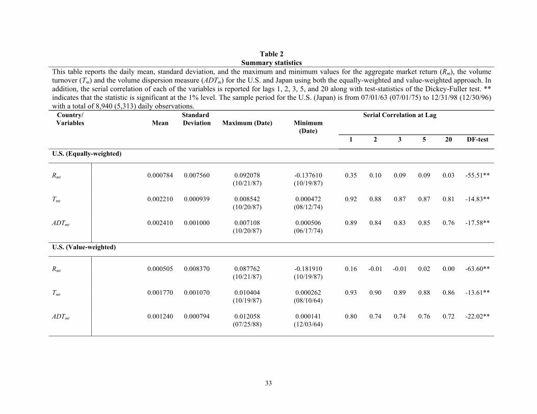
aggregate market level could be achieved by including the ADTmt measure. In Table 2, we provide descriptive

statistics of this measure. Our discussion will focus on the US data. Using the equally-weighted approach, the

mean value of ADTmt is 0.24% with a standard deviation of 0.10%. The corresponding figures using the value-

weighted approach are 0.12% and 0.08% respectively. Table 2 also reports summary statistics for the turnover

measure (Tmt). The mean value of Tmt is 0.22% (0.18%) for the equally-weighted (value-weighted) sample. The

Dickey-Fuller test for examining the non-stationarity of the equally-weighted ADT (Tmt) measure is rejected at

the 1% level with a value of -17.58 (-14.83). Likewise, for the value-weighted measure, the Dickey-Fuller test

statistic assumes a value of -22.02 (-13.61) for ADT (Tmt), which is significant at the 1% level.

is different across different securities, it will potentially impact the turnover dispersion measure. 19 Using U.S. data, Tkac (1999) demonstrates that S&P 500 firms, firms with significant institutional ownership, and firms with listed options are likely to trade more than the volume benchmark (used to adjust for the level of market-wide trading activity) would predict. This type of variability in firm-level characteristics can alter the price change-volume relation at the level of the aggregate market.

17

As mentioned earlier, we hypothesize a negative relation between ADTmt and market return in the up-market

and a positive relation in the down-market. Moreover, if the inclusion of ADTmt measure results in a more

correctly specified regression, then specification (10) may allow us to re-establish the price change-volume

relation observed at the individual security level for both the U.S. and Japan.

In general, the results presented in Table 3 are consistent with all of our conjectures. First, the addition of

the ADTmt measure in the return-volume equation at the aggregate market level increases the explanatory power

of the regression specification. For instance, in the case of the U.S (Japan) without including ADTmt, the

aggregate market level regression, which utilizes the equally-weighted approach, has an adjusted R2 of 0.47

(0.40) (Table 1, Panel A). The corresponding adjusted R2 values for the specification in the case of the U.S

(Japan), which includes both the ADTmt measure and the aggregate market turnover, i.e. Tmt, are 0.53 (0.44)

(Table 3, Panel A).

Second, we find that the estimated γ2UP coefficients are uniformly negative, and (as predicted) all estimated

γ2DOWN coefficients are positive. Moreover, all eight estimated coefficients are significant at the 1% level. The

results provide strong evidence in support of our intuition. The evidence also suggests that our ADTmt measure

provides us with a reasonable proxy for the time-varying component of aggregate trading generated by firm-

specific information.

Third, consistent with prior findings regarding individual securities, the γ1UP coefficients are significantly

positive. These results hold for both the equally-weighted and value-weighted measures (Table 3, Panel A) for

both the U.S. and Japanese equity markets. Hence, we provide evidence that the positive price change-trading

volume relation documented at the individual security level in the up-market also holds at the aggregate market

level. This finding is non-trivial. We could not confirm such a relationship in the case of Japan using the

equally-weighted market index (Table 1). Yet, by the inclusion of ADTmt, we have successfully re-established

the expected positive relation between Rmt and Tmt. Similarly, the results in Table 3 also show that, whereas

some of these estimated coefficients are either positive or insignificant in Table 1, the γ1DOWN coefficients are

significantly negative for all four market index level regressions.

Overall, the results in Table 3 significantly add to our understanding of the underlying return-volume

18

relation at the aggregate market level. We find that, conditional on ADTmt, the magnitude of the market index

returns is significantly correlated with the aggregate daily turnover. Furthermore, after controlling for ADTmt, the

relation between price change and trading volume becomes V-shaped, as shown by Karpoff (1987).

To check for the robustness of our results, we run separate regressions for the respective market

capitalization-based quintile portfolios for the two countries (Table 3, Panel B). Without exception, all of the

sub-sample results are consistent with those obtained at the aggregate market index level. While the above

analysis highlights the importance of including the ADTpt measure in analyzing the price change-volume relation

at the aggregate market level, its usefulness cannot be overlooked in examining the analogous relation for any

portfolio. The rationale is the same: the composite portfolio returns are affected by trading triggered by both

macroeconomic information and firm-specific information of its constituent securities. The effect of the latter is

likely to be captured by the ADTpt measure.

B. The relation between volatility and volume

In this section, we examine the contemporaneous relation between unconditional volatility and volume at

the aggregate market level [equation (12)]. In Table 4, we report regression results for the market indexes. The

expected positive relation between return volatility and trading volume fails to hold at the aggregate market

index level in three of the four regression specifications. In case of the U.S. (Japan), the volatility-volume

relation is positive but insignificant (negative and significant) for the equally-weighted market index and

positive and significant (positive but insignificant) for the value-weighted market index. These findings are

analogous to those reported earlier during our examination of the price change-volume relation. Our analysis in

Section III suggests that failure to include the ADTmt measure may result in a mis-specified regression model.

In Table 5, we add the ADTmt measure to the volatility-volume regressions as specified in equation (13). The

results indicate that both Tmt and ADTmt are significant determinants of market volatility. Again, the addition of

the ADTmt measure in the volatility-volume equation at the portfolio level significantly increases the explanatory

power of the equation. For instance, the aggregate market level regression for the U.S (Japan), which utilizes the

equally-weighted index, resulted in an increase in the adjusted R2 from 0.007 (0.008) to 0.019 (0.061). The

19

adjusted R2 in the case of the value-weighted index increased from 0.037 (0.0001) to 0.060 (0.102) for the U.S.

(Japan). Moreover, we find that the positive relation between market volatility and aggregate trading volume is

once again re-established for both indexes. The results indicate that the market days with higher return volatility

are associated with higher average trading volume (Tmt) and lower dispersion in abnormal trading volume

(ADTmt).20

Incidentally, these results are also consistent with the argument that, during periods of higher market

volatility, investors may ignore their own private information and trade with their herd instinct (Christie and

Huang (1995)). This would decrease the dispersion in abnormal turnover across individual securities but

increase aggregate market level turnover in both up and down-markets.21

The findings in Table 5 should be of particular interest to index option traders. Of course, what would be

even more useful to the index option traders is the predictability of index-level volatility. Our earlier results in

Table 2 indicate that both Tmt and ADTmt exhibit significant first-order autocorrelation. Therefore, it is plausible

that the lagged values of Tmt and ADTmt can offer additional power in predicting the next day’s index-level

volatility. In Table 6, we report the results of the relation between market volatility (proxied by |Rmt|), lagged

aggregate market turnover and lagged turnover dispersion to ascertain whether these variables have any power

in predicting future volatility [equation (15)]. We find that both γ1 and γ2 coefficients are statistically significant

in all regressions for the U.S. and Japan. Moreover, the coefficients have the same signs as the contemporaneous

relation. These results further highlight the importance of the ADTmt measure.

C. The relation between implied volatility, volume and dispersion

It is well recognized that volatility is the most important parameter in pricing options. As such, traders are

20 The positive sign on the volume coefficient is consistent with Wood, McInish and Ord (1985), Harris (1986), and Gallant, Rossi and Tauchen (1992). 21 Herd behavior could become increasingly important in instances where the market is dominated by large institutional investors. Since institutional investors are evaluated with respect to the performance of a peer group, they have to be cautious about basing their decisions on their own prior information and ignoring the decisions of other managers. Shiller and Pound (1989) demonstrate that institutional investors place significant weight on the advice of other professionals with regard to their buy-and-sell decisions for more volatile stock investments.

20

interested in all variables that can enhance the explanatory power of the model attempting to capture the time-

series variation in the underlying volatility. We demonstrate that the ADTmt variable proposed in this paper

supplements the role played by market trading volume as an additional determinant of market index volatility.

The results in Panel B of Table 5 indicate that the importance of ADTmt cannot be overlooked in examining the

analogous relation for any portfolio. Therefore, it could be a useful instrumental variable in understanding the

time-series behavior of market volatility.

The results in Table 5 and Table 6 are governed by the use of |Rmt| or |Rpt| as a proxy for market or portfolio

volatility. Of particular interest to options traders are the contemporaneous and predictive relations amongst the

implied volatility of index options, the turnover rate of the underlying component securities of the market index,

and turnover dispersion. To examine these relations more closely and to gauge the sensitivity of our results, we

apply the analysis using S&P 100 index options.

The implied volatility data (IV) for the S&P 100 index options used in this analysis is obtained from the

CBOE Volatility Index (VIX). The data spans the sample period from January 1986 to December 1998. To

construct the Tmt and ADTmt measures, we confine the sample firms to the constituent securities of the S&P 100

Index. Panel A of Table 7 reports the contemporaneous relation amongst IVt, Tmt and ADTmt. It shows that both

the coefficients on Tmt and ADTmt are highly significant for both the equally-weighted and value-weighted

measures, with adjusted R2 equal to 0.27 and 0.18 respectively. These findings suggest that both turnover and

dispersion measures contain useful information for options traders.

The results of the test of the predictive relation are reported in Panel B of Table 7. We find that the lagged

values of Tmt and ADTmt are also important predictors of the implied volatility of index options. Both variables

are highly significant and the adjusted R2 of the regression specification ranges from 0.18 to 0.26. These

findings confirm that the ADTmt measure developed in this study has practical merits in explaining and

predicting the implied volatility of traded index options.

In summary, an important lesson to be learnt from our empirical findings from the U.S. and Japan is that we

cannot directly apply the results of individual security level price change/volatility-volume relation to the

aggregate index level price change/volatility-volume relation. Incorporating a measure of the dispersion in the

21

flow of firm-specific information at the individual security level, to the aggregate market level analysis,

significantly increases the explanatory power of the index level price change/volatility-volume relation.

D. Instrumental variable analysis

In Table 3, we report the results of regression specification (10) estimated in conjunction with the up- and

down- market dummy variables. The reliability of the parameter estimates for equation (10) hinges on the

crucial assumption that Tmt is uncorrelated with the error term εmt. However, when turnover and returns are

jointly determined at time t, Tmt and εmt must be correlated. Such a correlation between a regressor and an error

term tends to produce biased and inconsistent parameter estimates and standard errors.

To address this potential problem, we re-estimate equation (10) using an instrumental variable approach.

The instruments that we choose are the lagged values of turnover and dispersion at time t-1. By definition, εmt is

a residual error that is uncorrelated with any variables prior to time t, including Tmt-1 and ADTmt-1. The

orthogonality conditions are thus satisfied. In order to implement the instrumental variable procedure, we first

regress Tmt (ADTmt) on Tmt-1 (ADTmt-1). The fitted value of Tmt (ADTmt) from the first stage regression is then used

as a regressor to estimate equation (10).

Table 8 provides the estimated results of equation (10) for U.S. and Japan using the instrumental variables

regression approach. Panel A indicates that the estimated coefficients are highly significant for both the equally-

weighted and value-weighted approach, and with the correct signs as hypothesized for up- versus down-market.

For the size-rank portfolios (Panel B), similar findings emerge. All but one of the estimated coefficients are at

least statistically significant at the 10% level. The only exception is the slope parameter, γ1down, corresponding to

Tpt of quintile portfolio 3 for the US sample. In general, the results of the instrumental variables regression are

qualitatively similar to those reported in Table 3.

We further replicate regression specifications in equations (13) and (14) using the same set of instruments.

These results are reported in Table 9. Analogous to the findings reported in Table 5, the absolute value of price

change is highly correlated with the instruments used for turnover and dispersion. Without exception, all of the

estimated regression parameters are statistically significant and with the appropriate signs as hypothesized.

22

We also examine the contemporaneous relation between the implied volatility of the S&P 100 index option,

volume turnover and turnover dispersion, using the fitted values of turnover and turnover dispersion (projected

respectively by their time t-1 counterparts) as instruments. These results are similar to the results reported in

Panel A of Table 7, and show a strong and significant contemporaneous relation between IVt, Tmt and ADTmt

with adjusted R2 of 0.27 (0.18) for the equally-weighted (value-weighted) sample. In addition the γ1 and γ2

coefficients are all significant at the 1% level, and with the anticipated signs.22 In other words, all of the results

reported in Table 3, 5 and 7 remain robust using the instrumental variable estimation technique.

V. Conclusion

The empirical relation between price changes and trading volume has received considerable attention in the

finance literature. At the individual security level, several studies have demonstrated that significant price

changes are typically associated with higher trading volume. Moreover, these studies find that price declines are

usually accompanied by relatively low trading volume whereas price increases are accompanied by relatively

high trading volume. Earlier researchers have also documented a positive association between return volatility

(proxied by the absolute value of price change) and trading volume. As a result, volume has become a

commonly used technical indicator among investment professionals. In addition, since volatility is one of the

most important determinants of underlying option values, trading volume is also monitored closely by many

option traders.

In this study, we examine the price change-volume relation at the market index level, and argue that it is

critical to draw a distinction between aggregate market level trading volume and the variation in trading volume

across the individual securities that comprise the market. To explicitly take the latter into consideration, we

propose a novel “turnover dispersion” measure. The use of the turnover dispersion measure is justified by the

argument that both market-wide information and firm-specific information cause trading. While the arrival of

market-wide information is likely to have a universal effect on the price and the trading volume of all securities,

22 The results pertaining to the implied volatility of the S&P 100 index option using the instrumental variable approach are

23

the arrival of firm-specific information, whether public or private, can vary greatly across the individual

securities that comprise the overall market. The turnover dispersion measure in our analysis is designed to

capture the differences in market-wide versus firm-specific information effects on the price change-volume

relation at the level of the aggregate market.

Using individual security level data from the U.S. and Japanese equity markets, we document a positive

(negative) price change-volume relation in up (down)-markets. However, the price change-volume relation

found at the individual security level does not always hold at the aggregate market level, but can be re-

established by the introduction of the turnover dispersion measure. In fact, we find a negative (positive) relation

between aggregate market returns and turnover dispersion in up (down)-markets, suggesting that large positive

or negative returns are associated with low levels of dispersion in firm-specific trading volume across individual

securities. In addition, the introduction of the turnover dispersion measure in the aggregate market level

regressions significantly improves the explanatory power of the regression specifications.

In examining the relation between market return volatility, trading volume, and turnover dispersion, we

uncover the presence of a positive relation between market volatility and trading volume, and a negative relation

between market volatility and turnover dispersion. These results remain robust across the various size-ranked

portfolios, regardless of whether the absolute value of the market return or the implied volatility for index

options is used as the volatility measure. Finally, we document that lagged values of market level trading

volume and turnover dispersion can predict the next day’s index-level volatility. This analysis suggests that

index option traders need to pay close attention to both aggregate market level trading volume and turnover

dispersion to better capture the dynamics of daily market volatility.

not formally reported in a table, but are available upon request.

24

References

Admati, A. and P. Pfleiderer, 1988, “A Theory of Intraday Patterns: Volume and Price Variability,” Review of Financial Studies, 1, 3-40. Bessembinder, H., K. Chan, and P. Seguin, 1996, “An Empirical Examination of Information, Differences of Opinion, and Trading Activity,” Journal of Financial Economics, 40, 105-134. Bikhchandani, S., Hirshleifer, D., and I. Welch, 1992, “A theory of fads, fashion, custom, and cultural change as informational cascades,” Journal of Political Economy 100, 992-1026. Blume, L., D. Easley, and M. O’Hara, 1994, “Market Statistics and Technical Analysis: The Role of Volume,” Journal of Finance, 49, 153-181. Campbell, J., S. Grossman, and J. Wang, 1993, “Trading Volume and Serial Correlation in Stock Returns,” Quarterly Journal of Economics, 108, 905-939. Chan, K. and W. Fong, 2000, “Trade Size, Order Imbalance, and the Volatility-Volume Relation,” Journal of Financial Economics, 57, 247-273. Christie, W. G., and R. D. Huang, 1995, “Following the pied piper: Do individual returns herd around the market?,” Financial Analysts Journal, 1995, 31-37. Conrad, J., A. Hameed, and C. Niden, 1994, “Volume and Autocovariances in Short-Horizon Individual Security Returns,” Journal of Fiannce, 49, 1305-1329. Copeland, T. E., 1977, “A Probability Model of Asset Trading,” Journal of Financial and Quantitative Analysis, November, 563-578. Copeland, T. and D. Galai, 1983, “Information Effects on the Bid-Ask Spread,” Journal of Finance, 38, 1457-1469. Daigler, R., and M. Wiley, 1999, “The Impact of Trade Type On the Futures Volatility-Volume Relation,” Journal of Finance, 54, 2297-2316. Devenow, A, and I. Welch, 1996, “Rational Herding in Financial Economics,” European Economic Review 40, 603-615. Epps, T. W., 1975, “Security Price Change and Transaction Volumes: Theory and Evidence,” American Economic Review, 65, 586-597. Epps, T., and M. Epps, 1976, “The Stochastic Dependence of Security Price Changes and Transaction Volume: Implications for the Mixture-of-Distributions Hypothesis,” Econometrica, 44, 305-321. Epps, T. W., 1977, “Security Price Change and Transaction Volumes: Some Additional Evidence,” Journal of Financial and Quantitative Analysis, 12, 141-146. Foster, F. D., and S. Viswanathan, 1993, “The Effect of Public Information and Competition on Trading Volume and Price Volatility,” Review of Financial Studies, 6, 23-56. Gallant, A. R., P. E. Rossi, and G. Tauchen, 1992, “Stock Prices and Volume,” Review of Financial Studies, 5,

25

199-242. Gervais, S., R. Kaniel, and D.H. Mingelgrin, 2001, “The High-Volume Return Premium,” Journal of Finance, 56, 877-919. Godfrey, M. D., Granger, C. W. J., and O. Morgenstern, 1964, “The Random Walk Hypothesis of Stock Market Behavior,” Kyklos, 17, 1-30. Gordon G. and G. Pennacchi, 1993, “Security Baskets and Index-Linked Securities,” Journal of Business, 66, 1-27. Granger, C. W. J., and O. Morgenstern, 1963, “Spectral Analysis of New York Stock Market Prices,” Kyklos, 16, 1-27. Harris, L, 1986, “Cross Security Tests of the Mixture of Distributions Hypothesis,” Journal of Financial and Quantitative Analysis, 21, 39-46. Harris, M., and A. Raviv, 1993, “Differences of Opinion make a Horse Race,” Review of Financial Studies, 6, 473-506. Holden, C. and A. Subrahmanyam, 1992, “Long-Lived Private Information and Imperfect Competition,” Journal of Finance, 47, 247-270. Jain, P. C., and G. Joh, 1988, “The Dependence between Hourly Prices and Trading Volume,” Journal of Financial and Quantitative Analysis, Vol. 23, No. 3, 269-283. Jennings, R., L. Starks, and J. Fellingham, 1981, “An Equilibrium Model of Asset Trading with Sequential Information Arrival,” Journal of Finance, 36, 143-161. Jones, C. M., G. Kaul, and M. Lipson, 1994a, “Information, Trading, and Volatility,” Journal of Financial Economics, 36, 127-154. Jones, C. M., G. Kaul, and M. Lipson, 1994b, “Transactions, Volume, and Volatility,” Review of Financial Studies, 7, 631-651. Kandel, E. and N. D. Pearson, 1995, “Differential Interpretation of Public Signals and Trade in Speculative Marketes,” Journal of Political Economy, Vol. 103, No. 4, 831-872. Karpoff, J. M., 1986, “A Theory of Trading Volume,” Journal of Finance, XLI, No. 5, 1069-1087. Karpoff, J. M., 1987, “The Relation between Price Changes and Trading Volume: A Survey,” Journal of Financial and Quantitative Analysis, 22, 109-114. Kim, O. and R. Verrecchia, 1991, “Market Reaction to Anticipated Announcements,” Journal of Financial Economics, 30, 273-309. Kyle, A., 1985, “Continuous auctions and Insider Trading,” Econometrica, 53, 1315-1335. Lakonishok, J., A. Shleifer, and R. W. Vishny, 1992, “The Impact of Institutional Trading on Stock Prices,” Journal of Financial Economics, 32, 23-43. Lamoureux, C., and W. Lastrapes, 1990, “Heteroscedasticity in Stock Return Data: Volume versus GARCH

26

Effects,” Journal of Finance, 45, 221-229. Lamoureux, C. and W. Lastrapes, 1994, “Endogenous Trading Volume and Momentum in Stock-Return Volatility,” Journal of Business and Economic Statistics, 12, 253-260. Lee, C. M. C., and B. Swaminathan, 2000, “Price Momentum and Trading Volume,” Journal of Finance, 55, 2017-2070. Llorente, G., R. Michaely, G. Saar, and J. Wang, 2002, “Dynamic Volume-Return relation of Individual Stocks,” Review of Financial Studies, 15, 1005-1047. Lo, A. and A. Mackinlay, 1990, “An Econometric Analysis of Nonsynchronous Trading,” Journal of Econometrics, 45, 181-211. Lo, A. and J. Wang, 2000, “Trading Volume: Definitions, Data Analysis, and Implications of Portfolio Theory,” Review of Financial Studies, 13, 257-300. McQueen, G., M. A. Pinegar, and S. Thorley, 1996, “Delayed reaction to good news and the cross-autocorrelation of portfolio returns,” Journal of Finance, 51, 889-919. Mech, T., 1993, “Portfolio Return Autocorrelation,” Journal of Financial Economics, 34, 307-344. Morgan, I., 1976, “Stock Prices and Heteroscedasticity,” Journal of Business, 49, 496-508. Morse, D., 1980, “Asymmetric Information in Securities Markets and Trading Volume,” Journal of Financial and Quantitative Analysis, 15, 1129-1148. Qi, R., 2001, “Return-Volume Relation in the Tail: Evidence from Six Emerging Markets,” Columbia University, Working Paper. Schwert, G., 1989, “Why Does Stock Volatility Change Over Time?” Journal of Finance, 44, 1115-1154. Shiller, R. J., and J. Pound, 1989, “Survey evidence of diffusing interest among institutional investors,” Journal of Economic Behavior and Organization 12, 47-66. Stickel, S., and R. Verrecchia, 1994, “Evidence that Volume Sustains Price Changes,” Financial Analyst Journal, 57-67. Tauchen, G., and M. Pitts, 1983, “The Price Variability-Volume Relationship on Speculative Markets,” Econometrica, 51, 485-505. Tkac, P. A., 1999, “A Trading Volume Benchmark: Theory and Evidence,” Journal of Financial and Quantitative Analysis, 34, 89-114. Varian, H., 1985, “Divergence of Opinion in Complete Markets: A Note,” Journal of Finance, 40, 309-317. Wang, J., 1993, “A Model of Intertemporal Asset Prices Under Asymmetric Information,” Review of Economic Studies, 60, 249-282. Wang, J., 1994, “A Model of Competitive Stock Trading Volume,” Journal of Political Economy, 102, 127-168.

27

Welch, I., 1992, “Sequential sales, learning and cascades,” Journal of Finance, 47 695-732. Wood, R. and T. McInish, and J. Ord, 1985, “An investigation of Transactions Data for NYSE Stocks,” Journal of Finance, 60, 723-739. Ying, C., 1966, “Stock Market Prices and Volumes of Sales,” Econometrica, 34, 678-685.

28

APPENDIX

As stated earlier, the objectives of this paper are empirically oriented and are aimed at broadening our

understanding of the price change and volume relation at the aggregate market level. In this Appendix, we

streamline our intuitive justification pertaining to the regression specification used in the analysis.

Our investigation begins with the following return (Rit) generating process for stock i on day t, which is

analogous to the traditional market model:

itmtiit RR εβ += i = 1, …, N (A1)

where N is the total number of securities in a market index, Rmt is the return on the market portfolio and εit is a

normally distributed random variable uncorrelated with Rmt. To capture our intuition, we assume that the trading

turnover (defined as the number of shares traded divided by the total number of shares outstanding) of security i

on day t, Tit, is driven by a common market-wide factor Fmt, and a firm-specific component | ωit| 23 That is,

ititmtiit FT νωα ++= || i = 1, …, N (A2)

where αi > 0 is firm i’s daily turnover rate response coefficient to the common factor Fmt and ωit is a random

variable with zero mean and νit is an error term.

Without loss of generality, in the spirit of Lamoureux and Lastrapes (1994), we further assume that

Ftmtmt RF ηδθ ++= || (A3)

where θ and δ are positive constants, and ηFt is a random number with zero mean which is uncorrelated with

|Rmt| and is restricted to ensure that Fmt is always non-negative. The specification is justified by an argument

similar to the mixture model of Tauchen and Pitts (1983). It imposes a restriction to equations (A1), (A2) and

(A3) where the macro information arrival, proxied by Rmt, is a common factor affecting both daily stock returns

and trading volume. Therefore, Rmt can be viewed as a proxy for the latent mixing variable of the mixture model,

which interprets the latent process as the number of daily (common) information arrivals to the market. As such,

equation (A2) can be re-written as

23 Decomposing total turnover into market-wide and firm-specific components to examine the price change-volume

29

ititFtimtiiit RT νωηαδαθα ++++= |||| (A4)

Based on equations (A1) and (A4) and by denoting each security’s weight in the index as wi, a weighted index

return RIt and index turnover TIt can be expressed as:

it

N

iiit

N

ii

N

iiiFt

N

iiimti

N

iiIt wwwwRwT νωαηαδαθ ∑∑∑∑∑

=====

++++=11111

|||| (A5)

∑∑==

+=N

iitii

N

iimtIt wwRR

11

εβ (A6)

When N is large, based on the diversification argument, the last terms in equations (A5) and (A6) can be ignored.

Let

. and 11

i

N

iii

N

ii wBwA βα ∑∑

==

==

By combining (A5) and (A6), and via a simple re-arrangement, we obtain the following equation:

( )θηδ

ωδ

+−

−= ∑

=Ft

N

iitiItIt

BwTABR

1

|||| (A7)

Several interesting observations arise from equation (A7). First, the last term is uncorrelated with |RIt|. Second,

the absolute value of the aggregate index return is positively correlated with TIt, but negatively correlated with

the weighted average of |ωit|. Third, by using Φ to represent (B/δA) and dichotomizing realized RIt into a positive

sub-sample and a negative sub-sample, we obtain the following equations:

( ) ( )θηδ

ω +

−Φ−Φ= ∑

=Ftit

N

iiItIt

BwTR ||1

for all RIt ≥ 0 (A8)

( ) ( )θηδ

ω +

+Φ+Φ−= ∑

=Ftit

N

iiItIt

BwTR ||1

for all RIt < 0 (A9)

In equation (A8), the last term, (ηFt + θ), again is uncorrelated with RIt. In a way, this equation is analogous to

equation (1) for an individual stock when the stock return is positive. In our case, it depicts the relationship

between RIt and TIt when the weighted index return is positive. The equation suggests that realized index returns

relation is similar in spirit to Tkac (1999), Llorente, Michaely, Saar, and Wang (2002), and Lo and Wang (2000).

30

are positively correlated with the weighted index turnover rates. However, it also suggests that realized index

returns are negatively correlated with the weighted sum of turnovers induced by firm-specific information of all

the constituent securities making up the index. In other words, given the same level of TIt, the index return RIt

will in general be relatively low when the contribution to TIt collectively made by firm-specific information is

relatively high. Only with the same degree of firm-specific information would one expect positive RIt to increase

monotonically with TIt. The same analysis with opposite signs is applicable to equation (A9).

31

Table 1 Market level analysis of the price change-volume relation

Panel A reports the estimated coefficients of the following regression model: Rpt = αup Dup + αdown Ddown + γ1

up Dup

Tpt + γ1 downDdown

Tpt + εpt Panel B reports the estimated coefficients of the following regression model:

Tpt = αup Dup + αdown Ddown + γ1up

Dup Rpt + γ1

downDdown Rpt + εpt

where Rpt is the return on market index p in time interval t and Tpt is the daily trading volume turnover of market index p. Dup = 1 if Rpt ≥ 0 and Dup = 0 otherwise. Ddown = 1 if Rpt < 0 and Ddown = 0 otherwise. We report regression results at the level of the aggregate market index using an equally-weighted and a value-weighted approach. The results are reported separately for the up and down market return days. Heteroscedasticity and autocorrelation consistent t-statistics are reported in parentheses. The F1 tests the null hypothesis that α

UP = -αDOWN for Panel A, and tests if α

UP = α

DOWN for Panel B. F2 tests the null hypothesis that γ1UP = - γ1DOWN. ** and * denote that the coefficient is significant at the 1% and 5% levels respectively.

Up-Market

Down-Market

Test Statistics

αUP γ1UP αDOWN γ1DOWN Adj-R2 F1 F2

Panel A: Market Index Level Results

U.S. Equally-weighted market index

0.0040 (12.08)**

0.396 (2.73)**

-0.0040 (-4.54)**

-0.711 (-1.51)

0.470

0.00

5.97*

Value-weighted market index

0.0038 (15.06)**

1.099 (8.08.)**

-0.0041 (-6.32)**

-0.997 (-2.42)*

0.499

1.81

0.75

Japan Equally-weighted market index

0.0051 (15.06)**

-0.0926 (-0.71)

-0.0084 (-18.67)**

1.8869 (9.32)**

0.402

57.75**

58.87**

Value-weighted market index

0.0045 (12.09)**

0.8699 (4.20)**

-0.0073 (-19.62)**

0.9586 (4.44)**

0.414

38.23**

45.93**

32

Table 1 (Cont’d) Market level analysis of the price change-volume relation

Up-Market

Down-Market

Test Statistics

αUP γ1UP αDOWN γ1DOWN Adj-R2 F1 F2

Panel B: Market Index Level Results

U.S. Equally-weighted market index

0.0022 (67.54)**

0.015 (2.97)**

0.0020 (43.98)**

-0.015 (-1.89)

0.851

95.50**

0.00

Value-weighted market index

0.0016 (43.85)**

0.040 (8.68)**

0.0015 (35.85)**

-0.027 (-4.04)**

0.741

0.04

13.52**

Japan Equally-weighted market index

0.0020(62.23)**

-0.0022 (-0.72)

0.0016 (52.84)**

0.0177 (5.20)**

0.837

202.24**

19.95**

Value-weighted market index

0.0016 (60.68)**

0.0108 (3.83)**

0.0014 (56.82)**

0.0086 (3.60)**

0.8168

52.80**

46.45**

33

Table 2 Summary statistics

This table reports the daily mean, standard deviation, and the maximum and minimum values for the aggregate market return (Rm), the volume turnover (Tm) and the volume dispersion measure (ADTm) for the U.S. and Japan using both the equally-weighted and value-weighted approach. In addition, the serial correlation of each of the variables is reported for lags 1, 2, 3, 5, and 20 along with test-statistics of the Dickey-Fuller test. ** indicates that the statistic is significant at the 1% level. The sample period for the U.S. (Japan) is from 07/01/63 (07/01/75) to 12/31/98 (12/30/96) with a total of 8,940 (5,313) daily observations.

Country/ Variables

Mean

Standard Deviation

Maximum (Date)

Minimum

(Date)

Serial Correlation at Lag

1 2 3 5 20 DF-test

U.S. (Equally-weighted)

Rmt

0.000784

0.007560

0.092078 (10/21/87)

-0.137610 (10/19/87)

0.35

0.10

0.09

0.09

0.03

-55.51**

Tmt

0.002210

0.000939

0.008542 (10/20/87)

0.000472 (08/12/74)

0.92

0.88

0.87

0.87

0.81

-14.83**

ADTmt

0.002410

0.001000

0.007108 (10/20/87)

0.000506 (06/17/74)

0.89

0.84

0.83

0.85

0.76

-17.58**

U.S. (Value-weighted)

Rmt

0.000505

0.008370

0.087762 (10/21/87)

-0.181910 (10/19/87)

0.16

-0.01

-0.01

0.02

0.00

-63.60**

Tmt

0.001770

0.001070

0.010404 (10/19/87)

0.000262 (08/10/64)

0.93

0.90

0.89

0.88

0.86

-13.61**

ADTmt

0.001240

0.000794

0.012058 (07/25/88)

0.000141 (12/03/64)

0.80

0.74

0.74

0.76

0.72

-22.02**

34

Table 2 (continued) Summary statistics

Country/ Variables

Mean

Standard Deviation

Maximum

(Date)

Minimum

(Date)

Serial Correlation at Lag

1 2 3 5 20 DF-test

Japan (Equally-weighted)

Rmt

0.000736

0.008200

0.084248 (10/21/87)

-0.136480 (10/20/87)

0.27

0.02

0.04

0.01

-0.02

-46.74**

Tmt

0.001820

0.000852

0.005894 (02/03/89)

0.000251 (01/04/93)

0.85

0.78

0.75

0.76

0.60

-16.21**

ADTmt

0.001830

0.000931

0.006150 (08/05/77)

0.000345 (08/04/92)

0.85

0.78

0.74

0.75

0.63

-16.32**

Japan (Value-weighted)

Rmt

0.000338

0.009370

0.100120 (10/21/87)

-0.143890 (10/20/87)

0.12

-0.06

-0.01

-0.03

-0.02

-52.06**

Tmt

0.001560

0.000763

0.006319 (03/27/86)

0.000207 (01/04/93)

0.77

0.66

0.62

0.62

0.49

-20.84**

ADTmt

0.001340

0.000754

0.005889 (06/01/89)

0.000234 (07/28/92)

0.81

0.71

0.66

0.66

0.57

-19.16**

35

Table 3 Market level analysis of the price change-volume and turnover dispersion relation

This table reports the estimated coefficients of the following regression model: Rpt = αup Dup + αdown Ddown + γ1

up Dup

Tpt + γ1 downDdown

Tpt + γ2up

Dup ADTpt + γ2

downDdown ADTpt + εpt

where Rpt is the return on the size-ranked portfolio p in time interval t, Tpt is the aggregate trading volume turnover of portfolio p, and ADTpt is the absolute value of the cross-sectional deviations in abnormal trading volume across individual firms that comprise the size-ranked portfolio (for the portfolio level regressions) and the market index (for the full sample regression). Dup = 1 if Rpt ≥ 0 and Dup = 0 otherwise. Ddown = 1 if Rpt < 0 and Ddown = 0 otherwise. We report regression results at the level of the aggregate market index using an equally-weighted and a value-weighted approach. We also report separate results of size-ranked quintile portfolios. For the formulation of the size-ranked portfolios, prior year-end market capitalizations are used. The results are reported separately for the up and down market return days. Heteroscedasticity and autocorrelation consistent t-statistics are reported in parentheses. The F1 , F2 and F3 statistics test the null hypotheses that α

UP = -αDOWN, γ1UP = - γ1DOWN and γ2UP = - γ2DOWN . ** and * denote that the

coefficient is significant at the 1% and 5% levels respectively.

Up-Market

Down-Market

Test Statistics

αUP γ1UP γ2UP αDOWN γ1DOWN γ2DOWN Adj-R2 F1 F2 F3

Panel A: Market Index Level Results

U.S.

Equally-weighted Market index

0.00497

(16.80)**

3.222

(9.37)**

-2.914

( –10.99)**

-0.00559

( –8.53**

-6.896

( –6.58)**

6.501

( 9.15)**

0.532

4.48*

160.26**

169.78**

Value-weighted Market index

0.00407 ( 16.88)**

2.185 (8.38)**

-1.757 ( –5.09)**

-0.00455 ( –7.77)**

-2.694 ( – 4.01)**

2.778 ( 4.94)**

0.512 3.87* 5.83* 12.66**

Japan

Equally-weighted Market index

0.0047

(15.07)**

5.8678

(7.65)**

-5.6686

( –7.75)**

-0.0080

( –18.29)**

-4.4352

( –4.12)**

6.1787

( 5.78)**

0.435

60.06**

3.58

0.53

Value-weighted Market index

0.0038

( 11.65)**

9.0215

( 11.93)**

-8.9022

( –11.59)**

-0.0062

( –17.36)**

-7.3156

( –8.78)**

8.7781

(9.99)**

0.473

27.44**

5.31*

0.03

36

Table 3 (continued) Market level analysis of the price change-volume and turnover dispersion relation

Up-Market

Down-Market

Test Statistics

αUP γ1UP γ2UP αDOWN γ1DOWN γ2DOWN Adj-R2 F1 F2 F3

Panel B: Quintile Portfolios Results

U.S.

Quintile Portfolio 1

(smallest)

0.00731

(16.40)**

1.068

(3.73)**

-0.614

( –3.37)**

-0.00672

( –10.40)**

-2.838

( –3.96)**

2.075

(6.94)**

0.472

2.38

27.86**

46.67**

Quintile Portfolio 2

0.00542 (12.72)**

1.887 (5.38)**

-1.300 ( –7.14)**

-0.00498 ( –5.12)**

-4.762 ( –4.58)**

3.368 (7.13)**

0.495 1.55 116.64** 136.12**

Quintile Portfolio 3

0.00507 (13.29)**

1.680 (6.86)**

-1.208 ( –9.57)**

-0.00500 ( –6.15)**

-3.486 ( –4.65)**

2.571 (7.13)**

0.508 0.05 58.22** 65.35**

Quintile Portfolio 4

0.00458 (15.65)**

1.858 (7.49)**

-1.441 ( –8.93)**

-0.00485 ( –7.76)**

-2.755 ( –4.40)**

2.197 ( 6.50)**

0.506 0.81 18.39** 16.86**

Quintile Portfolio 5 (largest)

0.00395 (16.60)**

2.013 (9.20)**

-1.551 ( –7.91)**

-0.00461 ( –8.39)*

-2.295 ( –3.22)**

2.153 (3.66)**

0.506 7.28** 2.28 6.88**

Japan

Quintile Portfolio 1

(smallest)

0.0047

(13.37)**

2.5211

(8.26)**

-2.0401

( –6.15)**

-0.0076

( –17.02)**

-1.3447

( –2.21)*

2.4822

(4.12)**

0.482

65.11**

8.59**

1.19

Quintile Portfolio 2

0.0052 (16.38)**

3.2753 (7.13)**

–3.1003 ( –6.75)**

-0.0077 ( –19.30)**

-5.0031 ( –6.81)**

6.0897 (8.29)**

0.437 41.56** 9.76** 32.02**

Quintile Portfolio 3

0.0053 (17.09)**

3.6710 (8.18)**

-3.5418 ( -7.89)**

-0.0079 ( –20.25)**

-4.2466 ( –6.26)**

5.3084 (7.95)**

0.444 36.37** 1.34 15.45**

Quintile Portfolio 4

0.0054 (16.35)**

3.6225 (8.55)**

-3.5925 ( –8.58)**

-0.0078 ( –22.34)**

-3.0700 ( –5.90)**

4.2337 (7.86)**

0.435 33.23** 1.52 2.45

Quintile Portfolio 5 (largest)

0.0053 (15.87)**

4.3482 (9.48)**

–4.4614 ( –8.42)**

-0.0070 ( –21.67)**

-2.6295 ( –7.36)**

3.5862 (8.27)**

0.448 16.63** 18.21** 4.55*

37

Table 4 Market level analysis of the volatility-volume relation

This table reports the estimated coefficients of the following regression model: |Rpt| = α + γ1 Tpt + εpt

where |Rpt| is the absolute value of the return on market index p in time interval t and Tpt is the daily trading volume turnover of market index p . We report regression results at the level of the aggregate market index, using an equally-weighted and a value-weighted approach. Heteroscedasticity and autocorrelation consistent t-statistics are reported in parentheses. ** and * denote that the coefficient is significant at the 1% and 5% levels respectively. Market Index Level Results U.S.

Equally-weighted market Index

0.0041 (8.29)**

0.472 (1.90)

0.007

Value-weighted market Index

0.0040 (10.42)**

1.051 (4.54)**

0.037

Japan Equally-weighted market Index

0.0064 (20.11)**

-0.6784 (-5.41)**

0.008

Value-weighted market Index

0.0058 (19.19)**

0.1453 (0.87)

0.0001

38

Table 5

Market level analysis of the volatility-volume and turnover dispersion relation This table reports the estimated coefficients of the following regression model:

|Rpt| = α + γ1 Tpt + γ2 ADTpt + εpt where |Rpt| is the absolute value of the return on the size-ranked portfolio p in time interval t, Tpt is the aggregatetrading volume turnover of portfolio p, and ADTpt is the absolute value of the cross-sectional deviations inabnormal trading volume across individual firms that comprise the size-ranked portfolio. We report regressionresults at the level of the aggregate market index using an equally-weighted and a value-weighted approach. Wealso report separate results of size-ranked quintile portfolios. For the formulation of the size-ranked portfolios,prior year-end market capitalizations are used. Heteroscedasticity and autocorrelation consistent t-statistics arereported in parentheses. ** and * denote that the coefficient is significant at the 1% and 5% levels respectively.

α

γ1 γ2 Adj-R2

Panel A: Market Index Level Results U.S.

Equally-weighted market index

0.00527 (11.86)**

4.618 (7.93)**

-4.271 (-10.73)**

0.019

Value-weighted market index

0.00429 (12.25)**

2.383 (6.40)**

-2.167 (-6.24)**

0.060

Japan

Equally-weighted market index

0.0059 (20.07)**

5.3371 (9.62)**

-5.7287 (-10.53)**

0.061

Value-weighted market index

0.0048 (18.45)**

8.4407 (14.58)**

-8.9323 (-14.93)**

0.102

Panel B: Quintile Portfolios Level Results U.S.

Quintile Portfolio 1 (smallest)

0.00693 (18.97)**

1.711 (4.85)**

-1.083 (-6.08)**

0.013

Quintile Portfolio 2

0.00531 (9.31)**

2.962 (5.06) **

-2.074 (-7.50)**

0.063

Quintile Portfolio 3

0.0517 (10.90)**

2.383 (6.02)**

-1.777 (-9.41)**

0.051

Quintile Portfolio 4

0.00477 (12.72)**

2.207 (6.33)**

-1.762 (-9.08)**

0.049

Quintile Portfolio 5 (largest)

0.00425 (12.77)**

2.126 (5.53)**

-1.804 (-5.85)**

0.059

Japan

Quintile Portfolio 1 (smallest)

0.0056 (18.18)**

2.3596 (7.14)**

-2.2361 (-6.42)**

0.029

Quintile Portfolio 2

0.0060 (21.12)**

3.7830 (8.56)**

-3.9181 (-8.80)**

0.049

Quintile Portfolio 3

0.0062 (22.33)**

3.9913 (9.99)**

-4.1922 (-10.37)**

0.071

Quintile Portfolio 4

0.0063 (22.80)**

3.4870 (10.45)**

-3.8407 (-11.11)**

0.070

Quintile Portfolio 5 (largest)

0.0061 (22.16)**

3.7043 (11.54)**

-4.1130 (-10.89)**

0.075

39

Table 6

Market level analysis of the volatility-lagged volume and turnover dispersion relation: Predictability tests

This table reports the estimated coefficients of the following regression model: |Rmt| = α + γ1 Tt-1 + γ2 ADTt-1 + εt

where |Rmt| is the absolute value of the return on the market index m in time interval t, Tt-1 is the t-1 periodaggregate trading volume turnover of the market index, and ADTt-1 is the t-1 period absolute value of the cross-sectional deviations in abnormal trading volume across individual firms that comprise the market index. Wereport regression results at the level of the aggregate market index using an equally-weighted and a value-weighted approach. Heteroscedasticity and autocorrelation consistent t-statistics are reported in parentheses. **and * denote that the coefficient is significant at the 1% and 5% levels respectively.

α

γ1 γ2 Adj-R2

U.S.

Equally-weighted market Index

0.0060 (17.01)**

2.2907 (4.39)**

-2.4310 (-6..77)**

0.033

Value-weighted market Index

0.0051 (17.55)*

1.0660 3.358)**

-0.9306 (-3.64)**

0.012

Japan

Equally-weighted market Index

0.0070 (21.46)**

3.5006 (7.13)**

-4.4500 (-9.09)**

0.051

Value-weighted market Index

0.0068 (23.29)**

4.9702 (10.54)**

-6.2473 (-12.07)**

0.054

40

Table 7 An Analysis of the Relation between Volume, Turnover Dispersion and the Implied

Volatility of S&P 100 Stock Index Options (01/03/1986 - 12/13/1998) Panels A and B report, respectively, the estimated coefficients of the following two regression models:

tttt ADTTIV εγγα +++= 21

tttt ADTTIV εγγα +++= −− 1211

where IV t is the implied volatility of S&P 100 Stock Index Options on day t, Tt is the aggregate trading volume turnover of the constituent stocks in the S&P 100 Stock Index, and ADTt is the absolute value of the cross-sectional deviations in abnormal trading volume across individual firms that comprise the index. We report regression results using an equally-weighted and a value-weighted approach. Heteroscedasticity and autocorrelation consistent t-statistics are reported in parentheses. ** and * denote that the coefficient is significant at the 1% and 5% levels respectively.

Panel A : Contemporaneous Test

α γ1 γ2 Adj-R2

Equally weighted

0.1042 (3.73)**

174.86 (10.69)**

-170.67 (-12.67)**

0.270

Value weighted

0.0916 (3.67)**

111.55 (5.10)**

-93.42 (-5.18)**

0.179

Panel B : Predictability Test

α γ1 γ2 Adj-R2

Equally weighted

0.1066 (4.01)**

174.09 (10.83)**

-170.56 (-12.75)**

0.264

Value weighted

0.0925 (3.79)**

111.40 (5.14)**

-93.67 (-5.23)**

0.177

41

Table 8 Market level analysis of the price change-volume and turnover dispersion relation using the instrumental variable estimation technique

This table reports the estimated coefficients of the following regression model: Rpt = = αup Dup + αdown Ddown + γ1

up Dup

Tpt + γ1 downDdown

Tpt + γ2up

Dup ADTpt + γ2

downDdown ADTpt + εpt

where Rpt is the return on the size-ranked portfolio p in time interval t, Tpt is the aggregate trading volume turnover of portfolio p, and ADTpt is the absolute value of the cross-sectional deviations in abnormal trading volume across individual firms that comprise the size-ranked portfolio (for the portfolio level regressions) and the market index (for the full sample regression). Dup = 1 if Rpt ≥ 0 and Dup = 0 otherwise. Ddown = 1 if Rpt < 0 and Ddown = 0 otherwise. To implement the instrumental variable procedure, we first regress Tpt (ADTpt) on Tpt-1 (ADTpt-1). The fitted value of Tpt (ADTpt) from the first stage regression is then used as regressor to estimate the above equation. We report regression results at the level of the aggregate market index using an equally-weighted and a value-weighted approach. We also report separate results of size-ranked quintile portfolios. For the formulation of the size-ranked portfolios, prior year-end market capitalizations are used. The results are reported separately for the up and down market return days. Heteroscedasticity and autocorrelation consistent t-statistics are reported in parentheses. The F1 , F2 and F3 statistics test the null hypotheses that α

UP = -α

DOWN, γ1UP = -γ1DOWN and γ2UP = - γ2DOWN . *** , ** , and * denote that the coefficient is significant at the 1% , 5% , and 10% level respectively.

Up-Market

Down-Market

Test Statistics

αUP γ1UP γ2UP αDOWN γ1DOWN γ2DOWN Adj-R2 F1 F2 F3

Panel A: Market Index Level Results

U.S.

Equally-weighted Market index

0.0058

(16.35)***

2.0837

(5.75)***

-2.2599

(-8.38)***

-0.0067

(-13.14)***

-3.1401

(-3.09)***

3.4246

(4.56)***

0.484

7.14***

10.29***

13.23***

Value-weighted Market index

0.0050 (6.75)***

1.1352 (4.39)***

-1.0052 (-3.50)***

-0.0055 (-14.91)***

-1.1626 (-2.20)**

1.3655 (2.63)**

0.487 2.72* 0.01 0.98

Japan

Equally-weighted Market index

0.0066

(16.67)***

2.2504

(6.81)***

-2.9785

(-8.28)***

-0.0081

(-15.50)***

-1.7884

(-3.34)***

3.3140

(6.97)***

0.417

9.93***

0.57

0.40

Value-weighted Market index

0.0066

(16.39)***

4.0003

(7.27)***

-4.8896

(-8.36)***

-0.0070

(-14.44)***

-3.4409

(-5.47)***

4.6432

(7.79)***

0.433

0.38

0.56

0.13

42

Table 8 (continued) Market level analysis of the price change-volume and turnover dispersion relation using the instrumental variable estimation technique

Up-Market

Down-Market

Test Statistics

αUP γ1UP γ2UP αDOWN γ1DOWN γ2DOWN Adj-R2 F1 F2 F3

Panel B: Quintile Portfolios Results

U.S.

Quintile Portfolio 1

(smallest)

0.0079

(15.65)***

1.9656

(4.43)***

-1.4932

(-4.25)***

-0.0087

(-20.18)***

-1.1376

(-2.03)**

1.5144

(4.75)***

0.470

3.68**

4.87**

0.01

Quintile Portfolio 2

0.0073 (15.32)***

1.5313 (3.51)***

-1.6719 (-6.30)**

-0.0089 (-15.70)***

-2.0517 (-2.09)**

2.5426 (4.09)***

0.469 12.72*** 2.67* 10.76***

Quintile Portfolio 3

0.0072 (16.36)***

0.6494 (2.28)**

-1.0586 (-5.99)***

-0.0081 (-12.11)***

-0.7820 (-1.24)

1.3445 (3.63)***

0.485 4.55** 0.22 1.28

Quintile Portfolio 4

0.0062 (18.02)***

0.9272 (3.68)***

-1.1983 (-6.49)***

-0.0068 (-13.35)***

-1.1040 (-1.94)*

1.4470 (3.63)***

0.484 2.70* 0.55 0.87

Quintile Portfolio 5 (largest)

0.0048 (16.39)***

1.0036 (3.23)***

-0.7420 (-2.32)**

-0.0055 (-18.92)***

-1.0048 (-1.75)*

1.0989 (1.80)*

0.481 6.89*** 0.00 1.40

Japan

Quintile Portfolio 1

(smallest)

0.0055

(14.78)**

1.9025

(8.53)***

-1.6528

(-6.94)***

-0.0072

(-14.86)***

-1.0714

(-2.54)***

1.8457

(5.00)***

0.469

18.44***

4.41**

0.24

Quintile Portfolio 2

0.0064 (16.88)***

1.8665 (7.02)***

-2.1559 (-7.44)***

-0.0080 (-16.20)***

-1.2508 (-2.30)**

2.3046 (4.66)***

0.418 12.41*** 1.74 0.13

Quintile Portfolio 3

0.0070 (17.82)***

2.13830 (7.09)***

-2.6270 (-8.33)***

-0.0086 (-17.68)***

-1.3149 (-3.72)***

2.5201 (7.08)***

0.425 10.17*** 3.23* 0.08

Quintile Portfolio 4

0.0069 (17.95)***

2.1809 (7.06)***

-2.7460 (-8.273)***

-0.0080 (-8.334)***

-1.3397 (-3.88)***

2.4231 (6.82)***

0.416 4.37** 3.35* 0.70

Quintile Portfolio 5 (largest)

0.0068 (17.66)***

2.4482 (6.97)***

-3.0838 (-7.22)***

-0.0069 (-17.62)***

-1.7045 (-4.77)***

2.4696 (6.41)***

0.420 0.10 2.45 1.96

43

Table 9 Market level analysis of the volatility-volume and turnover dispersion relation using the instrumental

variable estimation technique This table reports the estimated coefficients of the following regression model:

|Rpt| = α + γ1 Tpt + γ2 ADTpt + εpt where |Rpt| is the absolute value of the return on the size-ranked portfolio p in time interval t, Tpt is the aggregatetrading volume turnover of portfolio p, and ADTpt is the absolute value of the cross-sectional deviations inabnormal trading volume across individual firms that comprise the size-ranked portfolio. To implement theinstrumental variable procedure, we first regress Tpt (ADTpt) on Tpt-1 (ADTpt-1). The fitted value of Tpt (ADTpt) fromthe first stage regression is then used as regressor to estimate the above equation. We report regression results atthe level of the aggregate market index using an equally-weighted and a value-weighted approach. We also reportseparate results of size-ranked quintile portfolios. For the formulation of the size-ranked portfolios, prior year-endmarket capitalizations are used. Heteroscedasticity and autocorrelation consistent t-statistics are reported inparentheses. *** , ** , and * denote that the coefficient is significant at the 1%, 5%, and 10 % level respectively.

α

γ1 γ2 Adj-R2

Panel A: Market Index Level Results U.S.

Equally-weighted market index

0.0063 (17.26)***

2.4788 (4.39)***

-2.7217 (-6.77)***

0.033

Value-weighted market index

0.0052 (18.21)***

1.1479 (3.35)***

-1.1684 (-3.64)***

0.012

Japan

Equally-weighted market index

0.0072 (20.39)***

2.0823 (7.11)***

-3.1089 (-10.17)***

0.043

Value-weighted market index

0.0068 (20.35)***

3.7548 (9.09)***

-4.7794 (-10.74)***

0.041

Panel B: Quintile Portfolios Level Results U.S.

Quintile Portfolio 1 (smallest)

0.0080 (22.87)***

1.7482 (4.55)***

-1.5163 (-5.69)***

0.013

Quintile Portfolio 2

0.0080 (18.39)***

1.7010 (2.86) ***

-2.0023 (-5.58)***

0.028

Quintile Portfolio 3

0.0076 (16.94)***

0.6761 (1.79)*

-1.1710 (-5.47)***

0.013

Quintile Portfolio 4

0.0065 (18.36)***

0.9896 (2.90)***

-1.3025 (-5.74)***

0.011

Quintile Portfolio 5 (largest)

0.0051 (20.35)***

0.9962 (2.56)***

-0.8843 (-2.28)**

0.012

Japan

Quintile Portfolio 1 (smallest)

0.0060 (18.51)***

1.6822 (7.38)***

-1.7201 (-7.64)***

0.017

Quintile Portfolio 2

0.0070 (20.47)***

1.6673 (5.86)***

-2.2096 (-7.67)***

0.031

Quintile Portfolio 3

0.0077 (21.40)***

1.8486 (7.15)***

-2.6071 (-9.66)***

0.051

Quintile Portfolio 4

0.0074 (22.25)***

1.8613 (7.13)***

-2.6271 (-9.54)***

0.047

Quintile Portfolio 5 (largest)

0.0068 (21.94)***

2.1281 (7.80)***

-2.8096 (-8.57)***

0.032

T5 T4 T3 T2 T1

Ave

rage

rate

of r

etur

n (%

)

T1 T2 T3 T4 T5

Ave

rage

rate

of r

etur

n (%

)

T5 T4 T3 T2 T1 T1 T2 T3 T4 T5

Ave

rage

rate

of r

etur

n (%

)

Ave

rage

rate

of r

etur

n (%

)

Down-Market Up-Market

1.541.81

2.092.53

4.01

Panel A: US Sample Down-Market Up-Market

0.811.01

1.221.51

2.79

Panel B: Japan Sample Figure 1: The daily return observations of each individual firm are partitioned into turnover quintiles according to the size of the firm’s daily turnover during the sample period, with quintile T1 (T5) containing observations with the lowest (highest) turnover rate. The return observations within each of the 5 turnover quintiles are further partitioned into an up-market sample (positive daily return) and a down-market sample (negative daily return). Equally-weighted average returns are computed for each of the 10 turnover groups. The data for the US (Japan) sample is from CRSP (PACAP) over the period from 1963 to 1998 (1975 to 1996).

-4.15

-3.32 -3.12 -3.01

- 2.82

-2.21 -1.89 -1.76

-1.66 -1.51

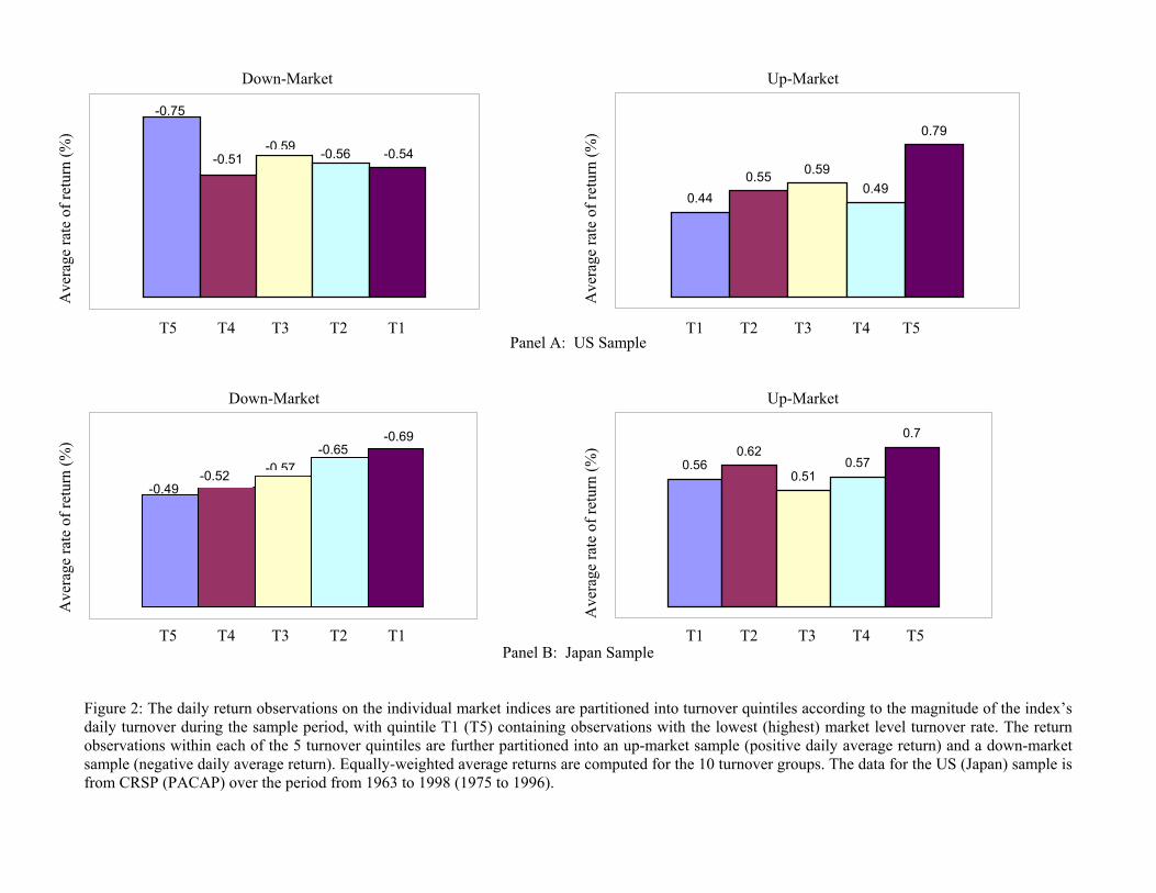
T5 T4 T3 T2 T1

T5 T4 T3 T2 T1

T1 T2 T3 T4 T5

T1 T2 T3 T4 T5

Ave

rage

rate

of r

etur

n (%

)

Ave

rage

rate

of r

etur

n (%

)

Ave

rage

rate

of r

etur

n (%

)

Ave

rage

rate

of r

etur

n (%

)

Down-Market Up-Market

0.440.55 0.59

0.49

0.79

Panel A: US Sample Down-Market Up-Market

0.560.62

0.510.57

0.7

Panel B: Japan Sample Figure 2: The daily return observations on the individual market indices are partitioned into turnover quintiles according to the magnitude of the index’s daily turnover during the sample period, with quintile T1 (T5) containing observations with the lowest (highest) market level turnover rate. The return observations within each of the 5 turnover quintiles are further partitioned into an up-market sample (positive daily average return) and a down-market sample (negative daily average return). Equally-weighted average returns are computed for the 10 turnover groups. The data for the US (Japan) sample is from CRSP (PACAP) over the period from 1963 to 1998 (1975 to 1996).

-0.75

-0.51 -0.59 -0.56 -0.54

-0.49 -0.52 -0 57

-0.65 -0.69

T5 T4 T3 T2 T1

T5 T4 T3 T2 T1

T1 T2 T3 T4 T5

T1 T2 T3 T4 T5

Ave

rage

rate

of r

etur

n (%

)

Ave

rage

rate

of r

etur

n (%

)

Ave

rage

rate

of r

etur

n (%

)

Ave

rage

rate

of r

etur

n (%

)

Down-Market Up-Market

0.41 0.450.54

0.62

0.86

Panel A: US Sample Down-Market Up-Market

0.360.45

0.520.64

0.95

Panel B: Japan Sample Figure 3: The daily returns on each market index are first partitioned into ADT (the absolute value of the cross-sectional deviations in abnormal turnover rate) quintiles according to the magnitude of daily ADT with quintile A1 (A5) containing observations with lowest (highest) ADT. Observations in each ADT quintile portfolio are further partitioned into turnover quintiles according to the magnitude of their daily turnovers, with quintile T1 (T5) containing observations with the lowest (highest) turnover rate. Observations in each cell of the 5 x 5 partition are further divided into up-market (positive daily market return) and down-market (negative daily market return) samples. For the up-market sample, the observations of five T1 portfolios are combined and an equally weighted average return is calculated for the combined portfolio. Similar averages are computed for the rest of the turnover quintile. The same aggregation and computation are conducted for the down-market sample.

-0.85

-0.62 -0.55 -0.50

-0.42

-0.88

-0.66

-0.53 -0.49 -0.49