The Role of Oscillatory Modes in U.S. Business Cycles

Andreas Grotha,b, Michael Ghila,b,c,∗, Stephane Hallegatted,e, Patrice Dumasd

aGeosciences Department, Ecole Normale Superieure, Paris, FrancebEnvironmental Research & Teaching Institute, Ecole Normale Superieure, Paris, FrancecDepartment of Atmospheric & Oceanic Sciences and Institute of Geophysics & Planetary

Physics, University of California, Los Angeles, USAdCentre International de Recherche sur l’Environnement et le Developpement,

Nogent-sur-Marne, FranceeEcole Nationale de la Meteorologie, Meteo France, Toulouse, France

Abstract

We apply multivariate singular spectrum analysis to the study of U.S. businesscycle dynamics. This method provides a robust way to identify and reconstructoscillations, whether intermittent or modulated. We show such oscillations tobe associated with comovements across the entire economy. The problem ofspurious cycles generated by the use of detrending filters is addressed and wepresent a Monte Carlo test to extract significant oscillations. The behavior ofthe U.S. economy is shown to change significantly from one phase of the businesscycle to another: the recession phase is dominated by a five-year mode, whilethe expansion phase exhibits more complex dynamics, with higher-frequencymodes coming into play. We show that the variations so identified cannot begenerated by random shocks alone, as assumed in ‘real’ business-cycle models,and that endogenous, deterministically generated variability has to be involved.

Keywords: Advanced spectral methods, Comovements, Frequency domain,Monte Carlo testing, Time domainJEL classification: C15, C60, E32

1. Introduction

Dominated over many decades by a long-term upward drift (Solow, 1956),macroeconomic time series also exhibit smaller but still important shorter-termfluctuations often associated with business cycles. The causes and characteris-tics of these cycles have been extensively studied in modern economic theory(Burns and Mitchell, 1946; Kydland and Prescott, 1998, and references therein).

A number of approaches have been proposed to separate the shorter-termfluctuations from the long-term trend (Canova, 1998; Baxter and King, 1999).Morley and Piger (2012) recently attempted a classification of business cycle

∗Corresponding author: Michael Ghil, ghil@lmd.ens.fr

Preprint submitted to JBCMA, accepted for publication March 25, 2014

analyses into (i) those that consider a cyclic sequence of expansions and contrac-tions; and (ii) an output-gap view, in which business cycles merely correspondto transitory fluctuations superimposed on a permanent trend level.

The definition of business cycles depends, however, on the knowledge of atrend component that cannot be observed directly. Several filters have been de-veloped (Graff, 2011) to extract such a trend component, of which the Hodrick-Prescott (HP) filter is the most commonly used one (Hodrick and Prescott,1997). Since there is no fundamental theory—and hence no generally accepteddefinition—of the trend, the resulting residuals have to be analyzed very crit-ically, to avoid spurious results due merely to the detrending procedure it-self (Nelson and Kang, 1981; Harvey and Jaeger, 1993; Cogley and Nason, 1995).

Business cycles can also be understood as comovements of transitory fluctu-ations in several distinct macroeconomic variables (Burns and Mitchell, 1946;Lucas, 1977). It is imperative, therefore, to analyze business cycle properties asa multivariate process.

The purpose of this paper is to apply multivariate singular spectrum analy-sis (M-SSA)—the extension of singular spectrum analysis (SSA) to multivari-ate time series—to the analysis of business cycles. Both SSA and M-SSArely on the classical Karhunen–Loeve spectral decomposition of random pro-cesses (Karhunen, 1946; Loeve, 1945, 1978). Broomhead and King (1986a,b)proposed to use both in the context of nonlinear dynamics as a more robust ap-plication of the Mane–Takens idea of reconstructing dynamics from measuredtime series (Mane, 1981; Takens, 1981; Sauer et al., 1991). Ghil, Vautard andassociates (Vautard and Ghil, 1989; Ghil and Vautard, 1991; Vautard et al.,1992) noticed that SSA can be used as a time-and-frequency domain methodfor the analysis of time series, whether they are generated by a linear stochasticprocess, a nonlinear deterministic one or a superposition of the two.

We propose to use M-SSA for the analysis of business cycles in a completelymultivariate fashion. This method combines two useful approaches of statisti-cal analysis: (1) it determines—with the help of principal component analysis(PCA)—major directions in the system’s phase space that are populated by themultivariate time series; and (2) it extracts major spectral components by usingdata-adaptive filters. To get reliable information about significant oscillatorymodes, we perform exhaustive statistical tests by means of Monte Carlo SSA(MC-SSA, Allen and Smith, 1996), which allow us to deal with the problem ofspurious oscillations (Nelson and Kang, 1981; Cogley and Nason, 1995).

SSA and M-SSA have already proven their advantages in a variety of appli-cations, such as climate dynamics, meteorology and oceanography, as well as thebiomedical sciences. Ghil et al. (2002) provide an overview and a comprehensiveset of references to their theory and applications. In economics, this approachhas received little attention so far. Recent applications to the univariate SSAanalysis of business cycles include de Carvalho et al. (2012), Sella and Marchion-atti (2012), and Dumas et al. (2013). The present paper introduces the M-SSAmethodology into the economic literature and demonstrates its advantages forthe multivariate analysis of economic activity.

The paper is organized as follows. In Section 2, we introduce the method-

2

ology and summarize its properties in terms of spectral decomposition, as wellas of time-domain reconstruction. In Section 3, we apply SSA to the U.S. grossdomestic product (GDP) and M-SSA to the full data set. The reliability ofthe results is then discussed via Monte Carlo testing. Section 4 analyzes thecycle-to-cycle variability of the U.S. business cycles, and we draw conclusionsabout the underlying dynamics in Section 5.

2. Decomposition and reconstruction

2.1. Data and pre-processing

We study here U.S. macroeconomic data from the Bureau of Economic Anal-ysis (BEA; see http://www.bea.gov). The nine variables analyzed are GDP,investment, employment rate, consumption, total wage, change in private in-ventories, price, exports, and imports; all monetary variables are in constant2005 dollars, while the employment rate is in percentage points. The quarterlytime series cover 52 years, from the first quarter of 1954 to the third quarter of2005.

Aligning ourselves with the output-gap view of business cycle analysis, wefirst remove the trend of each time series separately, by using the HP filter withthe common parameter value λ = 1600. Employment is the only one of thenine variables that does not exhibit an upward trend; still, we do detrend it toconsistently remove periods longer than 10 years, as done for the other variables.

The restriction to the interval 1954–2005 reduces end-to-end mismatches ofthe remaining transitory fluctuations and minimizes spectral leakage effects, i.e.the presence of spurious oscillations in the spectral analysis. On the macroeco-nomic side, the years 2007-2008 correspond to a well-known crisis, whose originwas financial, rather than economical. The time interval since that crisis exhib-ited several new characteristics, for which we do not yet have sufficiently longdata sets to distinguish this interval from the previous half-a-century of data.

In contrast to our two-step approach—see also Dumas et al. (2013)—de Car-valho et al. (2012) have chosen to apply a single SSA analysis for the decom-position of the GDP into trend and fluctuations. Such an approach is indeeddesirable as it appears to provide a more consistent separation into a perma-nent trend component and transitory fluctuations that are orthogonal to it (cf.Vautard et al., 1992; Ghil et al., 2002). In the present macroeconomic context,however, the trend dominates the SSA’s variance-based phase-space decompo-sition and small fluctuations could be masked in such a single-sweep analysis(Granger, 1966; Sella and Marchionatti, 2012). We will return to this issue inthe estimation of the covariance matrix in Sec. 2.2.

In line with our two-step decomposition, we next obtain trend residuals thatwe divide by the trend—i.e., we concentrate on relative values—and then trans-form to unit standard deviation. This normalization brings all the indicators tothe same scale and gives equal weight to each of them in the M-SSA analysis.One could choose to give different weights to each time series to reflect a prioriideas on their relative importance. Our choice here is one of simplicity, and the

3

(a) Pre−processed time series

−0.2

−0.1

0

0.1

0.2

(b) RCs 1−10 of M−SSA

−0.2

−0.1

0

0.1

0.2

(c) RCs 1−2 of PCA

1955 1960 1965 1970 1975 1980 1985 1990 1995 2000 2005

−0.2

−0.1

0

0.1

0.2

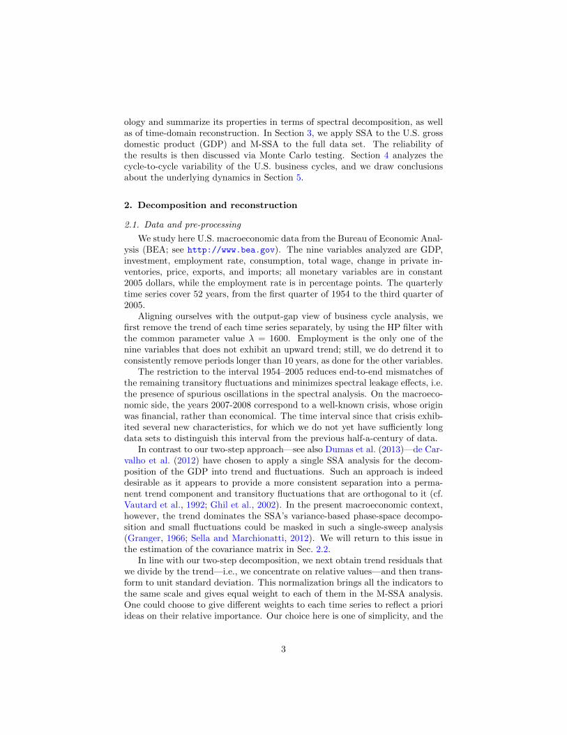
Figure 1: The nine time series of U.S. macroeconomic data used in this paper; raw data fromthe U.S. Bureau of Economic Analysis (BEA), 1954–2005. The figure illustrates the resultsof pre-processing and of applying either multivariate singular spectrum analysis (M-SSA) orprincipal component analysis (PCA); the shaded vertical bars in the three panels indicateNBER-defined recessions. (a) Detrended and standardized time series. (b,c) Reconstructionof the entire data set: (b) with the first 10 M-SSA components, using a window width ofM = 24 quarters; and (c) with the first two PCA components. Both reconstructions capture75% of the total variance, while the M-SSA reconstruction is smoother.

covariance matrix is transformed into a correlation matrix. Finally, we dividethe normalized time series by (DM)1/2—with D the number of variables andM the window width—so that the sum of the partial variances equals one.

Figure 1a shows the results of this pre-processing. The U.S. recessions, asdefined by the NBER, are indicated by shaded vertical bars.

2.2. Singular spectrum analysis (SSA)

In this section we discuss the univariate version of SSA and present its mainproperties, in particular, its ability to reconstruct cyclical dynamics.

Following Mane (1981) and Takens (1981), the starting point of SSA is toembed the time series {x(t) : t = 1, . . . , N} into an M–dimensional phase space

4

X, by using M lagged copies

x(t) =(x(t), x(t+ 1), . . . , x(t+M − 1)

), (1)

with t = 1, . . . , N−M+1. The SSA procedure starts by calculating the principaldirections of the embedded data set x(t).

Reconstructing the entire attractor of a nonlinear dynamical system fromx(t), as originally proposed by Broomhead and King (1986a), may fail, how-ever, even in relatively simple cases (Mees et al., 1987; Vautard and Ghil, 1989).Ghil, Vautard and several associates first proposed, instead, to apply the SSAmethodology to describe cyclical behavior in short and noisy time series, forwhich standard methods derived from Fourier analysis do not work well (Vau-tard and Ghil, 1989; Ghil and Vautard, 1991; Vautard et al., 1992). The keyidea in their approach was to reconstruct the ‘skeleton of the attractor,’ i.e. themost robust, albeit unstable limit cycles embedded in it.

The next step in SSA is to compute the auto-covariance matrix C of x.Vautard and Ghil (1989) proposed to estimate it by

ci,j =1

N − |i− j|

N−|i−j|∑t=1

x(t)x(t+ |i− j|), (2)

imposing a Toeplitz structure with constant diagonals: the entries ci,j of thematrix depend only on the lag |i− j|.

The eigenvalues λk and eigenvectors ρk of C, k = 1, . . . ,M , are obtained bysolving

Cρk = λkρk. (3)

The eigenvectors, which are pairwise orthonormal, span a new coordinate systemin the M–dimensional embedding space X, and each eigenvalue λk indicatesthe variance in the corresponding direction ρk. This computation helps us find,therefore, the major components of the system’s dynamical behavior.

The eigenvectors of such a Toeplitz matrix are necessarily either symmetricor anti-symmetric, and the method’s reliability in extracting oscillations is en-hanced therewith by using this form of C (Allen and Robertson, 1996). In thepresence of strong non-stationarity, the Toeplitz approach yields a slightly largerbias in the reconstruction of low-frequency activity than the original trajectoryapproach of Broomhead and King (1986a).

The latter approach relies on a singular-value decomposition of the trajectorymatrix x and is more appropriate for the analysis of trends (Ghil et al., 2002).Our focus here is on the transitory fluctuations and we rely therefore on theToeplitz approach for our analysis. de Carvalho et al. (2012) have found thetrajectory approach to be also adequate in their one-step identification of thepermanent trend and superimposed fluctuations in the U.S. business cycles.

By convention, the eigenvalues {λk, k = 1, . . . ,M} are arranged in descend-ing order, from the largest to the smallest variance, yielding a so-called “screediagram” of eigenvalues λk vs. order k. In this diagram, one often looks fora clear break in the slope to distinguish ‘signal’ from ‘noise.’ Such a break,

5

however, occurs mostly when the noise is actually white, with no temporal cor-relations at all. The signal-to-noise separation test has, therefore, to be modifiedin the presence of non-vanishing correlations, as done in Sec. 3 below.

Projecting the embedded time series x onto eigenvectors ρk yields the cor-responding principal components (PCs),

Ak(t) =

M∑j=1

x(t+ j − 1)ρk(j), k = 1, . . . ,M. (4)

Note that the sum above is not defined close to the end of the time series, whereN −M ≤ t ≤ N . It is customary, therefore, to consider the PCs as defined foronly N −M + 1 indices, which could start at t = M and end at N , or startat t = 1 but end at N −M + 1; most commonly they are plotted centered forM/2 ≤ t ≤ N −M/2, with M even (Ghil et al., 2002).

Finally, we can reconstruct parts of the time series that are associated witha particular eigenvector by

rk(t) =1

Mt

Ut∑j=Lt

Ak(t− j + 1)ρk(j), k = 1, . . . ,M, (5)

cf. Ghil and Vautard (1991) and Vautard et al. (1992). The values of thetriplet of integers (Mt, Lt, Ut) for the central part of the time series, M ≤ t ≤N −M + 1, are simply (M, 1,M); for either end they are given in Ghil et al.(2002). Each reconstructed component (RC) rk(t) associated with the varianceλk has a complete set of N indices, but with a reduced confidence in its valuesat either end of the time series.

Given any subset k ∈ K of eigenelements, we obtain the corresponding re-construction rK(t) by summing the RCs,

rK(t) =∑k∈K

rk(t). (6)

Typical choices of K are (i) K = {k : 1 ≤ k ≤ S}, where S is the statisticaldimension of the time series, cf. Vautard and Ghil (1989), i.e., the number ofstatistically significant components; or (ii) a pair of components (k0, k1) forwhich λk0 ≈ λk1 , and which may capture a cyclic mode (see Section 3). Thewhole set of RCs, K = {k : 1 ≤ k ≤ M}, gives the complete reconstruction ofthe time series.

In the following we refer to the common notation for the reconstructed com-ponent rk as RC k, and for a sum of several, consecutive RCs in Eq. (6) fromindex k to index k′ as RCs k–k′.

From the viewpoint of signal processing, the RCs can be considered as filteredtime series, with the eigenvectors being a set of data adaptive filters. BothEqs. (4) and (5) can be interpreted as a finite-impulse response (FIR) filter(Oppenheim and Schafer, 1989), with ρk being an FIR filter of length M . ThePCs obtained in Eq. (4) are time-reversed in Eq. (5), and the FIR filter is run

6

0 0.5 1 1.5 20

0.05

0.1

0.15

0.2

(a) Spectrum of eigenvalues

Frequency (cycles/year)

λ

0 0.5 1 1.5 2

0.05

0.1

0.15

0.2

0.25

0.3

0.35

Frequency (cycles/year)

(b) Power spectral density

PS

D

−20 0 20−0.02

0

0.02

0.04Covariance function

Time lag in quarters

Figure 2: Univariate spectral analysis of U.S. gross domestic product (GDP). (a) Eigenvaluespectrum of λk (filled circles) vs. dominant frequency of the associated eigenvector ρk, withwindow width M = 24 quarters; the error bars indicate the significance levels (cf. Sec. 3.1).(b) Power spectral density (PSD) estimate (solid line) using Welch’s averaged periodogrammethod, with a Hamming window of length 128 quarters and 75% overlap (Priestley, 1991);the dashed lines indicate the significance levels. Inset: Covariance estimates (solid line) andtheir significance levels (dashed lines). The upper and lower significance levels in both panelsand in the inset are derived from the 2.5% and 97.5% percentiles of 1000 surrogate time seriesfrom an AR(1) null hypothesis; see Sec. 3.1.

again through them. After this second filter pass, the correct chronological orderis restored by reversing the filtered result rk(t) once more. This procedure iscalled forward-backward filtering, and it is known to preserve the phase relations.Hence, each RC k and the original time series x(t) are in phase and the filteringacts only on the amplitude.

In designing an appropriate band-pass filter, Baxter and King (1999) require,in particular, that this “filter should not introduce phase shifts.” Unlike theirband-pass filter, with its data-independent weights chosen a priori, SSA is dataadaptive. The M filters are the eigenvectors of the auto-covariance matrix andprovide an optimal spectral decomposition of the time series, i.e., a maximumof the variance is captured by a minimal number of spectral components.

Following Vautard et al. (1992), we assign to each pair (λk,ρk) a frequency,given by the maximum of the Fourier transform of ρk. Plotting each eigenvaluevs. its dominant frequency provides a complementary perspective on SSA interms of an analogy with classical spectral analysis.

This analogy becomes more obvious when analyzing the trend residuals ofGDP (Figure 2). In the SSA analysis of panel (a), we observe a maximum inthe spectrum of eigenvalues at the usually reported mean business cycle lengthof 5–6 years, which agrees with the classical estimation of the power spectraldensity (PSD) in panel (b). For various PSD estimation algorithms that we havetested, we observe a maximum around the same period; at this point, though,the trend residuals are still subject to the Nelson and Kang (1981) criticismof spurious cycles. Therefore, we have to perform additional significance tests

7

before relying on the results, cf. Sec. 3.1.

2.3. Multivariate SSA (M-SSA)

M-SSA provides an extension of SSA to multivariate time series (Broomheadand King, 1986b; Kimoto et al., 1991; Keppenne and Ghil, 1993; Plaut andVautard, 1994). Let x(t) = {xd(t): d = 1, . . . , D; t = 1, . . . , N} be a vectortime series of length N , with D channels. In generalizing (2), we use the Dauto-covariances Cd,d, as well as the D × (D − 1) cross-covariances Cd,d′ to

form a grand covariance matrix C:

C =

C1,1 C1,2 . . . C1,D

C2,1 C2,2 . . . C2,D

...... Cd,d′

...CD,1 CD,2 . . . CD,D

. (7)

Here C is a DM ×DM matrix and the entries of the individual matrices Cd,d′

can be estimated as

(ci,j)d,d′ =1

N

min{N,N+i−j}∑t=max{1,1+i−j}

xd(t)xd′(t+ i− j). (8)

The denominator N depends on the range of summation, namely N = min{N,N+i− j} −max{1, 1 + i− j}+ 1.

As before we diagonalize the grand matrix C to yield its eigenvalues λk andeigenvectors ρk,

Cρk = λkρk, k = 1, . . . , DM. (9)

In contrast to SSA, the M-SSA eigenvectors ρk have now length DM , andare composed of D consecutive segments ρd

k, d = 1, . . . , D of length M . Thesesegments can be likewise interpreted as frequency-selective FIR filters, combinedhere into one multivariate filter ρk.

The associated PCs are single-channel time series that are computed byprojecting the multivariate time series x(t) onto ρk,

Ak(t) =

D∑d=1

M∑j=1

xd(t+ j − 1)ρdk(j), k = 1, . . . , DM. (10)

In addition to the summation j over time, as in Eq. (4), we get a second summa-tion d over the channels. This summation involves a classical PCA. In particular,setting M = 1 reduces M-SSA to PCA in D variables.

Finally, one can reconstruct parts of each time series xd(t) associated withits corresponding eigenvector segment ρd

k by (Plaut and Vautard, 1994)

rdk(t) =1

Mt

Ut∑j=Lt

Ak(t− j + 1)ρdk(j), k = 1, . . . , DM ; d = 1, . . . , D. (11)

8

This formula provides a set of DM RCs for each of the D time series and—depending on the information contained in the cross-covariances Cd,d′—the RCsof different time series may or may not be correlated. In this way, M-SSA helpsextract common spectral components from the multivariate data set, along withcomovements of the time series.

In Figure 1, we compare the pre-processed time series in panel (a) with theM-SSA reconstruction in panel (b), using the ten leading RCs, and with PCAreconstruction in panel (c), using the two leading RCs of the data set; the latterresults from Eq. (11) with M = 1. Both the M-SSA and PCA reconstructionscapture 75% of the total variance and extract coherent behavior manifest inthe nine economic variables. In contrast to PCA, the M-SSA results are muchsmoother, having removed irregular temporal fluctuations. It is especially theinclusion of temporal correlations that makes M-SSA superior to PCA in theextraction of dynamical behavior.

3. Oscillatory behavior and its statistical significance

The trend residuals in Figure 1 exhibit obviously more structure than purewhite noise; we need, therefore, a stringent test to decide whether the visu-ally apparent cyclical behavior can be attributed to random fluctuations or to amore regular oscillatory behavior, of possibly intrinsic origin. Cogley and Nason(1995), among others, have discussed in detail the effects of detrending, in par-ticular the possibility that it might give rise to spurious cycles; their discussionwas placed in the context of the detrending effect on a standard real businesscycle (RBC) model, with no oscillatory dynamics.

We follow Cogley and Nason (1995) and test against a first-order autoregres-sive process, AR(1), to verify the statistical significance of oscillations; this testis already well-established in the geosciences (Allen and Smith, 1996; Ghil et al.,2002). Since AR(1) processes exhibit maximum variance at zero frequency, de-trending with the HP filter may yield a possibly spurious maximum in the PSDat other frequencies, e.g. around the commonly reported business cycle lengthof 5-6 years.

3.1. Univariate time series: the GDP

We first focus on GDP alone, the most widely studied macroeconomic indi-cator. A Monte Carlo–type test consists in first fitting an AR(1) process X(t)to the scalar time series x(t) of interest,

X(t) = aX(t− 1) + σ0 ε(t), (12)

with ε(t) being Gaussian white noise of variance σ = 1, and then comparing thespectral properties of many realizations of X(t) with that of x(t).

We estimate the regression coefficient in Eq. (12) to be a = 0.82, and thevariance σ0 = 0.04, with the influence of the HP filter taken into account. Thatis, we choose the parameter a to minimize the mean-square distance between

9

the GDP covariance function (solid line in the inset of Figure 2b) and the HP-filtered AR(1) covariance function (dotted line), while to estimate σ0 we use theunbiased estimator proposed by Allen and Smith (1996) for short time series.Given the model parameters, we create a set of 1000 surrogate realizations oflength N from the AR(1) model, lowpass filter each with the HP filter, andnormalize it to the same variance as x(t). An additional division by the trend isnot necessary, since the innovations in the AR(1) process have constant variance.

In Figure 2b, we compare the PSD estimate of the GDP residuals (solid line)with that of the surrogate time series. Frequency-dependent significance levelsat the 2.5% and 97.5% quantiles (dashed lines) also show high power aroundfive years, and the PSD estimate of the GDP falls entirely between them.

Other PSD estimates, such as the maximum entropy or the multi-tapermethod (see Ghil et al., 2002, and references therein), confirm this finding andyield the conclusion that GDP residuals alone cannot be distinguished from thenull hypothesis of an HP-filtered AR(1) process. The high PSD values aroundfive years could be due to the detrending of an otherwise stable model withexogenous excitation, in complete agreement with the findings of Cogley andNason (1995) and Nelson and Kang (1981).

The same lack of statistical significance holds for the lag-covariance function,as expected from the Wiener-Khinchin theorem, according to which the PSD andthe lag-covariance function of a time series are related by the Fourier transform(Blackman and Tukey, 1958). The swing below zero for the surrogate timeseries is thus likewise due to the HP filter’s effect; see the inset in Figure 2b.The preliminary conclusion is that we cannot falsify the null hypothesis of anAR(1) process for the GDP residuals, as analyzed separately here.

This conclusion can also be confirmed by MC-SSA, which tests whether aneigenvalue λk captures more partial variance in the direction of the correspond-ing eigenvector ρk than present in the null hypothesis. To derive significancelevels, the covariance matrix CS for each surrogate time series xS(t) is projectedonto the set of eigenvectors E of the original time series via

ΛS = EᵀCSE; (13)

here the eigenvectors ρk are the columns of E, and (·)ᵀ denotes the transposeof a matrix.

Equation (13) is not the eigendecomposition of CS, and ΛS is not necessarilydiagonal, as it would be for C. Instead, ΛS provides a measure of the discrep-ancy between CS and C, and by computing quantiles of the diagonal elements’distribution from a set of ΛS, we derive significance levels for each eigenvalueλk (Allen and Smith, 1996).

The resulting significance levels for the SSA analysis of GDP in Figure 2aare indicated as vertical bars and we see that all eigenvalues fall within theseerror bars. Hence, the observed spectrum of eigenvalues cannot falsify the nullhypothesis either. In the following subsection, we show that additional infor-mation from other macroeconomic indicators helps reject the null hypothesis.

10

Table 1: Null-hypothesis parametersVariable AR(1) parameters Time lag behind GDP

ad σd ∆d (quarters)GDP 0.82 0.040 0

Investment 0.92 0.028 1Employment 0.96 0.021 0

Consumption 0.88 0.034 0Total wage 0.95 0.024 0

∆(Inventories)∗ 0.61 0.055 0Price 0.99 0.012 7

Exports 0.95 0.023 1Imports 0.83 0.039 1

∗ Changes in inventories

3.2. Multivariate time series

To test significance in M-SSA results, comovements should be taken intoaccount in formulating the null hypothesis. Vector AR models, however, maysupport oscillations even for order one; when present, these are referred to asprincipal oscillation patterns (von Storch et al., 1995; Penland and Matrosova,2001). We keep, therefore, the idea of fitting univariate AR(1) processes

Xd(t) = adXd(t− 1) + σd εd(t), (14)

but build characteristics of the cross-correlations into the null hypothesis. Theestimated parameters for each indicator are listed in Table 1.

The cross-correlation information is included by coupling the noise residualsεd(t) at a certain temporal lag ∆d. Relative to GDP, denoted by x1(t), we chose∆d so as to maximize the correlations between x1(t) and xd(t+∆d). Doing so isespecially necessary for the price, for which we observe a correlation maximumat seven quarters (cf. Figure 3g).

The covariance matrix R for innovation processes εd(t) has elements

Rd,d′ =1

Nd,d′

min{N,N+∆d′−∆d}∑t=max{1,1+∆d′−∆d}

xd(t)xd′(t+ ∆d′ −∆d) ; (15)

the denominator Nd,d′ depends on the range of summation, namely Nd,d′ =min{N,N + ∆d′ −∆d} −max{1, 1 + ∆d′ −∆d} + 1. Cholesky decompositionyields R = LᵀL and we derive correlated innovation processes from

(ε1(t), . . . , εd(t+ ∆d), . . . , εD(t+ ∆D))ᵀ

= Lᵀ(ξ1(t), . . . , ξd(t), . . . , ξD(t))ᵀ,(16)

with the ξd’s being independent white-noise processes. Finally, we pass the real-izations through the HP filter and normalize it to the same standard deviationas the data set.

11

−2

0

2

4

x 10−3

(a) GDP − GDP (b) GDP − Investment (c) GDP − Employment

−2

0

2

4

x 10−3

(d) GDP − Consumption (e) GDP − Total wage (f) GDP − ∆(Inventories)

−20 −10 0 10 20

−2

0

2

4

x 10−3

(g) GDP − Price

Time lag in quarters−20 −10 0 10 20

(h) GDP − Exports

−20 −10 0 10 20

(i) GDP − Imports

Figure 3: Auto- and cross-covariance functions of the nine U.S. economic indicators withrespect to GDP (solid lines). Dashed lines indicate the significance levels 2.5% and 97.5%,as well as the median from the realization of 1000 surrogate time series. Panels (a)–(i) arelabeled directly in the figure; ∆(Inventories) in the legend of panel (f) indicates changes ininventories.

12

0 0.5 1 1.5 20

0.05

0.1

0.15

0.2

Frequency (cycles/year)

λ

Figure 4: Spectrum of M-SSA eigenvalues (non-dimensional, filled circles) using all nine U.S.indicators, with M = 24. The error bars indicate the significance levels, derived from the2.5% and 97.5% percentiles of 1000 multivariate surrogate time series.

Figure 3 compares the covariance of the data with that of the null hypothe-sis. Lead–lag relations among economic indicators are reproduced by the null-hypothesis model, and the data covariance function lies almost, but not quite,within the variability of the null hypothesis. As in the univariate case, the HPfilter introduces a swing below zero and which would lead once again to spuriouscycles.

Projecting the grand covariance matrix CS for each of the surrogate realiza-tions onto the data eigenvectors, ΛS = EᵀCSE, yields again a measure of thediscrepancy between CS and C, which allows us to derive significance levels forλk from the distribution of the diagonal elements of ΛS (Figure 4).

As in the case of GDP alone, we observe higher significance levels near afive-year period, but this time the data eigenvalues clearly exceed the uppersignificance level. Hence the high variance associated with the leading pairs ofeigenvalues can no longer be explained by spurious cycles induced by inappro-priate detrending.

We have further tested the consistency of the present results by using dif-ferent values of the window width, namely M = 20, 30, 40 and 50. It turns outthat the leading pair describes a significant oscillation of five-year period. Thethree-year oscillation in the second pair is somewhat less robust, but probablystill deserves further examination in future work.

We have performed additional, exhaustive tests—as proposed by Allen andSmith (1996)—to cope with the problem of overestimating large eigenvalues inSSA and have found further evidence that the five-year oscillatory pair is indeedstatistically significant at the 95% level. We focus, therefore, in the next sectionon this oscillatory mode and investigate its role in business cycle dynamics.

13

4. Business cycle dynamics: phase dependence and evolution

The presence of oscillatory pairs indicates recurrent behavior in the system’sdynamics. Such more-or-less regular recurrences are typically produced by thepresence of an attracting or only weakly unstable limit cycle in the dynam-ics (Vautard and Ghil, 1989; Vautard et al., 1992; Ghil et al., 2002). On theother hand, vector AR(1) processes can possess oscillatory solutions as well, asmentioned at the beginning of Section 3.2. In practice, however, it might behard to distinguish between purely deterministic, but chaotic oscillators andstochastically driven ones.

From the point of view of economic theory, the distinction is not that im-portant: in fact, deterministic mechanisms—whether linear or nonlinear—arethe only ones that give rise to cyclic behavior in a vector AR(1) process orin a vector random process generated by a system of linear (Arnold, 1974) ornonlinear (Arnold, 1998) stochastic differential equations as well (Schuss, 1980);for illustration purposes, we discuss the case of a vector AR(1) process in theAppendix. The stochastic forcing, if present, only contributes truly irregularfluctuations. It is, therefore, only the deterministic part of the dynamics that isof genuine interest in discussing cyclicity in macroeconomics, whether stochasticforcing is present or not.

The first two eigenvalues capture 40% of the total variance, and RCs 1-2 givealready a good approximation of the GDP, cf. Figure 5a. To better understandthe role of this five-year oscillatory mode in the processes of expansion andrecession, we study the temporal evolution of its variance.

Plaut and Vautard (1994) introduced the concept of local variance fractionVK(t),

VK(t) =

∑k∈KAk(t)2

DM∑k=1

Ak(t)2

, (17)

which quantifies the fraction of the total variance that is described by a subset Kof PCs in a window of length M . We consider the PCs as centered, i.e. startingat M/2, cf. Section 2.2.

Figure 5 shows this index, along with the NBER-defined recessions, for theleading PCs 1–2 in panel (b) and for PCs 3–150 in panel (c). The sum ofPCs 1–150 capture 99% of the total variance; see dash-dotted line in panel(b). Starting after 1980, it is quite remarkable that the fraction of the five-yearoscillatory mode in PCs 1–2 is high during recessions and low during expansions.It shows that during the recessions, the trajectory of the data set stays closer toa suspected five-year limit cycle—like the one in the Non-Equilibrium DynamicModel (NEDyM) of Hallegatte and Ghil (2008) or in other endogenous businesscycle models (Chiarella et al., 2005)—while this trajectory reveals more complexbehavior during expansions.

During the 1970s, PCs 1–2 capture roughly 50% of the variance or more overthe full decade, while from 1980 on, PCs 1–2 play a significant role only duringrecessions. This result of our analysis suggests a change in the system’s dynamics

14

(a) GDP and its reconstruction with M−SSA RCs 1−2

−0.2

−0.1

0

0.1

0.2

(b) Local variance fraction of M−SSA PCs 1−2

0

0.2

0.4

0.6

0.8

1

(c) Local variance fraction of M−SSA PCs 3−150

0

0.2

0.4

0.6

0.8

1

(d) Local variance fraction of PCA PCs 1−2

1960 1965 1970 1975 1980 1985 1990 1995 2000 20050

0.2

0.4

0.6

0.8

1

Figure 5: (a) Pre-processed GDP data set (light solid line) and its reconstruction with RCs1–2 of our M-SSA analysis (heavy solid line). (b,c,d) Local variance fraction V (t): (b) forM-SSA PCs 1–2 (solid line) and PCs 1–150 (near-total variance, dash-dotted line); (c) forM-SSA PCs 3–150 (solid line); and (d) for PCs 1–2 of a PCA analysis (light solid line), aswell as after smoothing with a two-year moving average (heavy solid line). The dashed linesin panels (b) and (c) give the 2.5%, 25%, 50%, 75%, and 97.5% percentiles based on 1000surrogate time series. The shaded vertical bars indicate NBER-defined recessions.

15

in the 1980s, a change that agrees in timing with the “great moderation,” duringwhich volatility in GDP growth diminished markedly (Kim and Nelson, 1999;McConnell and Perez-Quiros, 2000; Stock and Watson, 2002; Kim et al., 2004).

There has been considerable debate on the cause of this shift, as well ason the expected duration of the U.S. economy’s new mode of functioning; inparticular it has been proposed that this moderate behavior terminated in 2007,i.e. before and during the “great recession” of 2008–2009. In any case, ourresults are at least consistent with the hypothesis of structural changes in the1980s, and our M-SSA methodology can help provide sophisticated analysis toolsto determine whether and when the great moderation ended, once additionalBEA data become available.

To assess the significance of the local variance results, we compare theirvariability with that of the null hypothesis in Eq. (14). To wit, we project eachsurrogate realization onto the data eigenvectors ρk to obtain surrogate PCsin the same way as for the data set in Eq. (10). As in the significance testof the eigenvalues, the resulting surrogate PCs are not orthogonal, since theircovariance matrix ΛS is not diagonal.

For each surrogate PC we calculate the local variance fraction in the sameway as for the data set in Eq. (17), and derive time-dependent significance levelsfrom the distribution of VK(t) (Figs. 5b,c, dashed lines). Since the AR(1) pro-cesses are stationary, these levels are supposed to be constant; this stationarityis seen in fact in Figure 5, except near the end of the time series, i.e. startingat t ' N −M .

In contrast to the approximate constancy of VK(t) in the null hypothesis, thefive-year oscillatory mode in the data set exhibits much greater variance duringthe recessions, when it does exceed the 97.5% significance level. The variance inPCs 3–150 is also larger than can be explained by the null hypothesis, with VK(t)values that are significantly larger than the 97.5% percentile during expansionsand smaller than the 2.5% percentile during recessions, respectively.

We have further examined the variability of VK(t) during the whole 1954–2005 interval by using other quantities, such as standard deviation and in-terquartile range (not shown here). All these estimates confirm that the U.S.macroeconomic indicators exhibit larger variability than can be explained bythe random fluctuations of the null hypothesis.

It is interesting to note that a similar phenomenon can also be identifiedby applying PCA to the data (Figure 5d). Although, at first glance, the localvariance fraction of the leading two PCs of PCA (light solid line) is ratherirregular, with no apparent link to the business cycle, smoothing with a two-year moving-average filter (heavy solid line) does indeed produce a behaviorcomparable to that in Figure 5b. It would, however, be difficult to guess thatfrom the raw PCA results: the moving-average filtering was only inspired bythe M-SSA results in panels (b) and (c), which did not require any additionalpost-processing.

16

5. Concluding remarks

In this article, we applied multivariate singular spectrum analysis (M-SSA)to study business cycles dynamics in a consistent and multivariate way. OurM-SSA results allowed us to reconcile and combine the NBER definition of re-cessions with quantitative analysis. This methodology extends, in particular,the recently proposed SSA business cycle analysis of a single macroeconomicindicator (de Carvalho et al., 2012; Sella and Marchionatti, 2012; Dumas et al.,2013). The present M-SSA analysis uses information on nine U.S. macroeco-nomic indicators from the BEA for 52 years (1954–2005).

This extended business cycle analysis leads to three major conclusions: (i) thepresence of genuine periodicity in macroeconomic behavior and its determinis-tic causes; (ii) the essential role of comovements of economic aggregates in theproper definition of business cycles; and (iii) the dependence of economic ‘volatil-ity’ on the phase of the business cycle. We describe these conclusions in greaterdetail below.

Genuine periodicity and its deterministic causes. In their work about the ‘realfacts’ and monetary myths of business cycles, Kydland and Prescott (1998)discussed the origin of business cycles in terms of the Slutzky (1937) theoryof random shocks. In the simplest RBC models, cyclicity originates exclusivelyfrom productivity shocks that can be modeled by a simple random walk. Cogleyand Nason (1995) have, moreover, argued that the spurious appearance of busi-ness cycle dynamics can be generated by the HP filter even if none is present,even in a random walk.

In agreement with the findings of Cogley and Nason (1995), a simple uni-variate analysis of GDP does not reveal any significant oscillatory modes (seeFigure 2). Our multivariate analysis, however, uses a larger amount of infor-mation about macroeconomic behavior, and allows us to identify a five-yearoscillatory mode with high statistical confidence (see Figure 4). This mode can-not be explained by artificial effects due to detrending by the HP filter, and arandom-walk–driven model of business cycles has to be questioned in the lightof the results obtained in our paper.

A major result of our study thus points to the presence of deterministic,endogenous effects in the business cycles of the U.S. economy and leads tothe conclusion that business cycles cannot be explained by exogenous shocksalone. This conclusion does not exclude the importance of random effects in theeconomy, as discussed at the beginning of Section 4 and in the Appendix: it onlyemphasizes the role of the deterministic ones in giving rise to cyclic behavior.

Comovements of macroeconomic aggregates. The role of the additional infor-mation provided by the M-SSA analysis emphasizes the need to understandbusiness cycles as a phenomenon that is not limited to GDP variations, but in-volves all aspects of the economy; it is reflected, therefore, in the comovementsof several macroeconomic aggregates. In the present study, we have performed aquantitative analysis of the BEA data set that is consistent with the NBER defi-nition of the business cycle, inasmuch as it is entirely multivariate and takes into

17

account the lead-and-lag relationships between the various indicators present inthe data (see Table 1 and Figure 3). These lead-and-lag relationships, in turn,reflect certain widely acknowledged “stylized facts” of economic cycles (Kydlandand Prescott, 1998; Zarnowitz, 1985).

State-dependent fluctuations. M-SSA also allowed us to provide further insightinto the underlying macroeconomic dynamics, and especially into the crucialquestion of the complex interplay between endogenous dynamics and exogenousshocks. We showed that the U.S. economy changes its behavior from one phaseof the business cycle to another: the recession phase is dominated by the five-year mode, while the expansion phase exhibits more complex dynamics, withhigher-frequency modes coming into play (see Figure 5). This type of behaviorcannot be explained by the random fluctuations that drive a simple stationaryRBC model, in the absence of endogenous oscillatory dynamics.

It thus appears that the dynamics of the U.S. economy can indeed be de-composed into a five-year cycle and more complex, higher-frequency behaviorsuperimposed on this cycle. The amplitude of the latter, irregular componentis higher during expansions, i.e. the business cycle is more volatile during ex-pansions than during recessions.

This phase-dependent volatility is consistent with the response to naturaldisasters predicted by Hallegatte and Ghil (2008) in an endogenous businesscycle (EnBC) model. These authors have shown that exogenous shocks, whetherpositive or negative, are likely to have a bigger impact in the presence of EnBCs.

Their modeling framework (Hallegatte et al., 2008), while highly simplified,has Keynesian features and their EnBC model’s predictions can be interpretedin terms of production being closer to capacity during expansions. On the otherhand, the lower volatility during recessions in our analysis here is consistent withthe predicted reduction in sensitivity to exogenous shocks, due to underutilizedproduction capacity in the low phases of an EnBC. This so-called “vulnerabilityparadox” was also highlighted by Ghil et al. (2011) and by Dumas et al. (2013).

Such a variable-volatility pattern may seem at odds with the findings ofFrench and Sichel (1993). But this apparent discrepancy can be explained bythe fact that our analysis and theirs are not defining the fluctuations in thesame manner. French and Sichel (1993) modeled the variance of the residualson a long-term trend, without decomposing these residuals into cyclical andnon-cyclical behavior, as we do here, and found higher variance during epochsof recession. In the present paper, we study the fluctuations superimposed onthe sum of the long-term trend, plus a possible cyclical component. It is thevariance of the fluctuations so defined that is largest during expansions.

The next step in our research program is to investigate whether the changein the economy’s dynamical behavior between boom and bust also leads todifferent types of response to exogenous shocks. This question is fundamentalin attempting to evaluate the efficiency of economic policy in different phasesof the business cycle.

18

Acknowledgments

It is a pleasure to thank J.-C. Hourcade for informative and stimulating dis-cussions and J. H. Stock for detailed and constructive comments on an earlierversion of the paper. This work was supported by a CNRS post-doctoral fellow-ship to AG, the Groupement d’Interet Scientifique (GIS) Reseau de Recherchesur le Developpement Soutenable (R2DS) of the Region Ile-de-France, and theChaire Developpement Durable of the Ecole Polytechnique.

Appendix. Cyclicity in deterministic and stochastic models

It is well known, as already mentioned at the beginning of Section 3.2, thatvector AR(1) processes can posses oscillatory solutions, due to the presence of

pairs of complex conjugate eigenvalues (λk, λk+1) = (λ(r)k ± λ

(i)k ) in the spectrum

of the matrix A = (aij) that characterizes such a process,

X(t) = A X(t− 1) + Σ ε(t) ; (A.1)

here Σ is a covariance matrix multiplying the noise vector ε. For a stationary

AR(1) process, all the real parts λ(r)k of the eigenvalues of A must be negative,

and the damped oscillations are maintained at a statistically constant amplitudeby the noise ε.

In practice, such a stochastically driven oscillator might be hard to distin-guish from a purely deterministic, possibly chaotic one. But the term A X(t−1)in the former case, on the right-hand side of Eq. (A.1), still captures the man-ifestation of a coupled pair of deterministic feedbacks, one positive, the othernegative, whether linear or nonlinear, noise-driven or not, as the ultimate cause

of any complex conjugate pair of eigenvalues (λ(r)k ± λ

(i)k ).

References

Allen, M. R., Robertson, A. W., 1996. Distinguishing modulated oscillationsfrom coloured noise in multivariate datasets. Climate Dynamics 12 (11), 775–784.

Allen, M. R., Smith, L. A., 1996. Monte Carlo SSA: Detecting irregular oscilla-tions in the presence of colored noise. Journal of Climate 9, 3373–3404.

Arnold, L., 1974. Stochastic Differential Equations: Theory and Applications.J. Wiley.

Arnold, L., 1998. Random Dynamical Systems. Springer.

Baxter, M., King, R. G., 1999. Measuring business cycles: Approximate band-pass filters for economic time series. Review of Economics and Statistics 81 (4),575–593.

19

Blackman, R. B., Tukey, J. W., 1958. The Measurement of Power Spectra.Dover.

Broomhead, D. S., King, G. P., 1986a. Extracting qualitative dynamics fromexperimental data. Physica D 20 (2-3), 217–236.

Broomhead, D. S., King, G. P., 1986b. On the qualitative analysis of experi-mental dynamical systems. In: Sarkar, S. (Ed.), Nonlinear Phenomena andChaos. Adam Hilger, Bristol, England, pp. 113–144.

Burns, A. F., Mitchell, W. C., 1946. Measuring Business Cycles. NBER, NewYork City, New York.

Canova, F., 1998. Detrending and business cycle facts. Journal of MonetaryEconomics 41 (3), 475–512.

Chiarella, C., Flaschel, P., Franke, R., 2005. Foundations for a DisequilibriumTheory of the Business Cycle. Cambridge: Cambridge University Press.

Cogley, T., Nason, J. M., 1995. Effects of the Hodrick-Prescott filter on trendand difference stationary time series: Implications for business cycle research.Journal of Economic Dynamics and Control 19 (1-2), 253–278.

de Carvalho, M., Rodrigues, P. C., Rua, A., Jan. 2012. Tracking the US businesscycle with a singular spectrum analysis. Economics Letters 114 (1), 32–35.

Dumas, P., Ghil, M., Groth, A., Hallegatte, S., 2013. Dynamic coupling of theclimate and macroeconomic systems. Mathematics of the Social Sciences, inpress.

French, M. W., Sichel, D. E., Jan. 1993. Cyclical patterns in the variance ofeconomic activity. Journal of Business & Economic Statistics 11 (1), 113–119.

Ghil, M., Allen, M. R., Dettinger, M. D., Ide, K., Kondrashov, D., Mann,M. E., Robertson, A. W., Saunders, A., Tian, Y., Varadi, F., Yiou, P., 2002.Advanced spectral methods for climatic time series. Reviews of Geophysics40 (1), 1–41.

Ghil, M., Vautard, R., 1991. Interdecadal oscillations and the warming trend inglobal temperature time series. Nature 350 (6316), 324–327.

Ghil, M., Yiou, P., Hallegatte, S., Malamud, B. D., Naveau, P., Soloviev, A.,Friederichs, P., Keilis-Borok, V., Kondrashov, D., Kossobokov, V., Mestre,O., Nicolis, C., Rust, H., Shebalin, P., Vrac, M., Witt, A., Zaliapin, I., 2011.Extreme events: Dynamics, statistics and prediction. Nonlinear Processes inGeophysics 18, 295–350.

Graff, M., 2011. International business cycles: How do they relate to Switzer-land? Tech. Rep. 291, KOF Swiss Economic Institute, ETH Zurich WorkingPaper.

20

Granger, C. W. J., 1966. The typical spectral shape of an economic variable.Econometrica 34 (1), 150–161.

Hallegatte, S., Ghil, M., 2008. Natural disasters impacting a macroeconomicmodel with endogenous dynamics. Ecological Economics 68 (1–2), 582–592.

Hallegatte, S., Ghil, M., Dumas, P., Hourcade, J.-C., 2008. Business cycles,bifurcations and chaos in a neo-classical model with investment dynamics.Journal of Economic Behavior & Organization 67 (1), 57–77.

Harvey, A. C., Jaeger, A., 1993. Detrending, stylized facts and the businesscycle. Journal of Applied Econometrics 8 (3), 231–247.

Hodrick, R. J., Prescott, E. C., 1997. Postwar U.S. business cycles: An empiricalinvestigation. Journal of Money, Credit and Banking 29 (1), 1–16.

Karhunen, K., 1946. Zur Spektraltheorie stochastischer Prozesse. AnnalesAcademiæ Scientiarum Fennicæ. Ser. A1, Math. Phys. 34.

Keppenne, C. L., Ghil, M., 1993. Adaptive filtering and prediction of noisymultivariate signals: An application to subannual variability in atmosphericangular momentum. International Journal of Bifurcation and Chaos 3, 625–634.

Kim, C.-J., Nelson, C. R., 1999. Has the U.S. economy become more stable? aBayesian approach based on a Markov-switching model of the business cycle.Review of Economics and Statistics 81, 608–616.

Kim, C.-J., Nelson, C. R., Piger, J., Jan. 2004. The less-volatile U.S. economy: ABayesian investigation of timing, breadth, and potential explanations. Journalof Business & Economic Statistics 22 (1), 80–93.

Kimoto, M., Ghil, M., Mo, K.-C., 1991. Spatial structure of the extratropical40-day oscillation. In: Eighth Conference on Atmospheric and Oceanic Wavesand Stability (Denver, Colo.). American Meteorological Society, Boston,Mass., pp. 115–116.

Kydland, F. E., Prescott, E. C., 1998. Business cycles: Real facts and a mon-etary myth. In: James E. Hartley, Kevin D. Hoover, K. D. S. (Ed.), RealBusiness Cycles: A Reader. Routledge, pp. 231–247.

Loeve, M., 1945. Fonctions aleatoires de second ordre. Comptes Rendus del’Academie des sciences Paris 220, 380.

Loeve, M., 1978. Probability Theory, Vol. II, 4th ed. Vol. 46 of Graduate Textsin Mathematics. Springer-Verlag.

Lucas, R. E., 1977. Understanding business cycles. Carnegie-Rochester Confer-ence Series on Public Policy 5 (1), 7–29.

21

Mane, R., 1981. On the dimension of the compact invariant sets of certain non-linear maps. In: Dynamical Systems and Turbulence. Vol. 898 of LectureNotes in Mathematics. Springer-Verlag, Berlin, pp. 230–242.

McConnell, M. M., Perez-Quiros, G., 2000. Output fluctuations in the UnitedStates: What has changed since the early 1980’s? American Economic Review90 (5), 1464–1476.

Mees, A. I., Rapp, P. E., Jennings, L. S., 1987. Singular-value decompositionand embedding dimension. Physical Review A 36 (1), 340–346.

Morley, J., Piger, J., 2012. The asymmetric business cycle. Review of Economicsand Statistics 94 (1), 208–221.

Nelson, C. R., Kang, H., 1981. Spurious periodicity in inappropriately detrendedtime series. Econometrica 49 (3), 741–751.

Oppenheim, A. V., Schafer, R. W., 1989. Discrete-time signal processing.Prentice-Hall, Inc. Upper Saddle River, NJ.

Penland, C., Matrosova, L., 2001. Expected and actual errors of linear inversemodel forecasts. Monthly Weather Review 129, 1740–1745.

Plaut, G., Vautard, R., 1994. Spells of low-frequency oscillations and weatherregimes in the Northern Hemisphere. Journal of the Atmospheric Sciences51 (2), 210–236.

Priestley, M., 1991. Spectral Analysis and Time Series. Academic Press.

Sauer, T., Yorke, J. A., Casdagli, M., 1991. Embedology. Journal of StatisticalPhysics 65 (3-4), 579–616.

Schuss, Z., 1980. Theory and Applications of Stochastic Differential Equations.J. Wiley.

Sella, L., Marchionatti, R., 2012. On the cyclical variability of economic growthin Italy, 1881–1913: a critical note. Cliometrica, 1–22.

Slutzky, E., 1937. The summation of random causes as a source of cyclic pro-cesses. Econometrica 5, 105–146.

Solow, R., 1956. A contribution to the theory of economic growth. Journal ofEconomics 70(1), 65–94.

Stock, J. H., Watson, M. W., 2002. Has the business cycle changed and why?In: Gertler, M., Rogoff, K. S. (Eds.), NBER Macroeconomics Annual. MITPress, Cambridge, Mass., pp. 159–218.

Takens, F., 1981. Detecting strange attractors in turbulence. In: DynamicalSystems and Turbulence. Vol. 898 of Lecture Notes in Mathematics. Springer,Berlin, pp. 366–381.

22

Vautard, R., Ghil, M., 1989. Singular spectrum analysis in nonlinear dynamics,with applications to paleoclimatic time series. Physica D 35 (3), 395–424.

Vautard, R., Yiou, P., Ghil, M., 1992. Singular-spectrum analysis: A toolkit forshort, noisy chaotic signals. Physica D 58 (1-4), 95–126.

von Storch, H., Burger, G., Schnur, R., von Storch, J.-S., 1995. Principal oscil-lation patterns : a review. Journal of Climate 8 (3), 377–400.

Zarnowitz, V., 1985. Recent work on business cycles in historical perspective:A review of theories and evidence. Journal of Economic Literature 23 (2),523–580.

23