The Role of Nonlinear Factor-to-Indicator Relationships in Tests ofMeasurement Equivalence

Daniel J. BauerUniversity of North Carolina

Measurement invariance is a necessary condition for the evaluation of factor mean differencesover groups or time. This article considers the potential problems that can arise for tests ofmeasurement invariance when the true factor-to-indicator relationship is nonlinear (quadratic)and invariant but the linear factor model is nevertheless applied. The factor loadings andindicator intercepts of the linear model will diverge across groups as the factor meandifference increases. Power analyses show that even apparently small quadratic effects canresult in rejection of measurement invariance at moderate sample sizes when the factor meandifference is medium to large. Recommendations include the identification of nonlinearrelationships using diagnostic plots and consideration of newly developed methods for fittingnonlinear factor models.

Keywords: measurement, invariance, nonlinear, factor analysis, structural equation modeling

Measurement invariance refers to the equivalent measure-ment of a construct or set of constructs in two or moregroups or over time via a common instrument (i.e., a set ofobserved variables or indicators). When measurement in-variance holds, differences observed between groups orover time reflect true differences on the constructs of inter-est. If measurement invariance does not hold, however, anyobserved differences might simply reflect inequities of mea-surement and not true differences on the relevant constructs(Horn & McArdle, 1992; Meredith, 1993; Ployhart & Os-wald, 2004). Establishing measurement invariance has thusbecome an integral area of psychometric research. Withinthe factor analytic tradition, early attention was focused onthis issue by Meredith (1964). More recently, this literaturehas expanded greatly by reformulating questions of mea-surement invariance within a confirmatory factor analytic orstructural equation modeling approach (Joreskog, 1971;Meredith, 1993; Sorbom, 1974).

Studies of measurement invariance usually involve thecomparison of independent samples, typically two. A mul-tiple-groups confirmatory factor analysis is then used to testthe tenability of equality constraints on various componentsof the measurement model (e.g., factor loadings, indicator

intercepts, residual variances), often in a sequential fashion(Bollen, 1989, pp. 355–369; Widaman & Reise, 1997). Lesscommon are tests of longitudinal invariance, wherein asingle sample is administered the same measurement instru-ment on multiple occasions (Meredith & Horn, 2001; Van-denberg & Lance, 2000). Although procedures for testingmeasurement invariance are by now well established inpractice, several methodological issues continue to receiveattention. These include the relation of within- and between-group measurement properties (Borsboom, Mellenbergh, &Van Heerden, 2002; Lubke, Dolan, Kelderman, & Mellen-bergh, 2003), the use and power of equivalence tests(Cheung & Rensvold, 2002; Meade & Lautenschlager,2004), the permissibility of differences in indicator inter-cepts (Millsap, 1998), and the difficulties that may arisewhen only a subset of indicators function equivalently overgroups or time (i.e., partial invariance; Byrne, Shavelson, &Muthen, 1989; Cheung & Rensvold, 1999; Millsap &Kwok, 2004; Steenkamp & Baumgartner, 1998).

The purpose of this article is to consider an issue that hasheretofore received comparatively little attention in themeasurement invariance literature. Specifically, the factoranalysis model used to evaluate measurement invarianceassumes that the relationships of the observed measures tothe factors are linear. In the single-sample context, pro-nounced nonlinearity in these relationships may occur if, forinstance, the manifest variables are dichotomous or ordinaland incorrectly treated as continuous. In such instances,difficulty factors may emerge in the linear factor model(McDonald, 1967; Wherry & Gaylord, 1944) and morepreferable alternatives are to analyze polychoric correla-

Additional materials are on the Web at http://dx.doi.org/10.1037/1082-989X.10.3.305.supp

Correspondence concerning this article should be addressed toDaniel J. Bauer, Department of Psychology, Campus Box 3270,University of North Carolina at Chapel Hill, North Carolina27599-3270. E-mail: dbauer@email.unc.edu

Psychological Methods2005, Vol. 10, No. 3, 305–316

Copyright 2005 by the American Psychological Association1082-989X/05/$12.00 DOI: 10.1037/1082-989X.10.3.305

305

tions or to use nonlinear item response models (Joreskog &Moustaki, 2001; Mislevy, 1986; Muthen, 1984; Muthen &Christoffersson, 1981; Waller, Tellegen, McDonald, &Lykken, 1996). However, even with continuous observedvariables, the relationships between the factors and indica-tors may not be strictly linear. A key implication of thelinear model is that the strength of the relationship betweena factor and measured variable is constant at least within theobserved range of the data. This would not be the case if, forinstance, there was a floor or ceiling effect for the measureor, more generally, if increasing levels of the latent factorproduce either diminishing or increasing differences in themeasured variable reflecting the factor. For example, inmaking ratings of aggression, observers might have greaterdifficulty judging differences in low levels of aggressionthan in high levels of aggression. Similarly, Mooijaart andBentler (1986) comment that, for attitude scale data, partic-ipants often provide more extreme opinion ratings (at theends of the scale) than would be expected on the basis of alinear model.

Methods for estimating nonlinear factor analysis modelshave been available for many years and have recently seenrapid developments (see Wall & Amemiya, in press, for areview). These methods are rarely implemented in practice,however, despite the availability of specialized software(Etezadi-Amoli & McDonald, 1983; Wall & Amemiya, inpress). Such neglect may reflect the view that minor depar-tures from linearity are relatively innocuous, as a linearmodel will still provide a useful first-order approximation tothe true function. However, when the goal of the investiga-tion is to evaluate measurement invariance, a linear approx-imation can present certain difficulties. Namely, in thisarticle, I will demonstrate that if the factor-to-indicatorrelationship is invariant but evinces some curvature and ifthe factor means differ over groups, then the loadings andintercepts obtained by fitting a linear factor model willdiffer, causing invariance tests to be rejected. Power curvesshow that at modest sample sizes, even seemingly minorcurvature in factor-to-indicator relationships can lead torejection of factorial invariance in a linear factor model ifthe factor mean difference is of modest to large size. Al-though this exposition is focused on between-groups tests ofmeasurement invariance, similar problems would arise inlongitudinal tests of measurement invariance.

Consequences of Unmodeled Nonlinearity forFactorial Invariance

Let us begin by considering a relatively simple five-indicator latent factor model for a single sample. Denotingthe indicators as x1 through x5 and the latent factor as �, themodel for person i may be written as

�x1i

x2i

x3i

x4i

x5i

� � ��1

�2

�3

�4

�5

� � ��1

�2

�3

�4

�5

��i � ��1i

�2i

�3i

�4i

�5i

� . (1)

This model is, in effect, a simultaneous linear regression ofeach indicator on the latent factor and hence the symbols �,�, and � simply designate regression intercepts, slopes(loadings), and residuals. A key point for this article is thatthe regression of each indicator on the latent factor isassumed to be linear in form.

A more general expression for the factor model is

xi � � � ��i � �i. (2)

Here, xi is a p � 1 vector of scores on p manifest variables(or factor indicators) for individual i, � is a p � 1 vector ofindicator intercepts and � is a p � q matrix of factorloadings describing the regression of the manifest variableson the q latent common factors in the q � 1 vector �i. Thep � 1 vector �i holds the indicator residuals net the influ-ence of the common factors. These residuals include bothvariability due to random measurement error and true-scorevariability that is unique to each indicator. In addition, thedistribution of the latent factors �i is captured via the q � 1vector of latent means � and q � q covariance matrix �.The residuals �i are assumed to have zero expectation and ap � p covariance matrix �. The latent factors and residualsare assumed to be uncorrelated.

Under these assumptions, the model-implied mean vectorand covariance matrix of x are given as

� � � � ��

� � ���� � �. (3)

It is important to note that not all parameters in �, �, �, �and � can be estimated. One reason is that the latent factors,being unobserved, have no natural metric, and hence theirmeans and variances are arbitrary. There are two commonchoices for establishing the scale of the latent factors. Thefirst choice is to set the mean and variance of the factor tozero and one, respectively, thus standardizing the factor.The second possibility is to choose a particular indicator toanchor the scale of the latent factor by setting the interceptand loading of this indicator to zero and one, respectively(e.g., setting �1 � 0 and �1 � 1 for the model in Equation1). The latent factor then draws its (unstandardized) metricfrom the scaling indicator.

In addition to setting the scale of the latent variables, eachparameter in the model must be uniquely identified by themeans, variances, and covariances of the indicators. That is,there must be sufficient information in the data to locate asingle optimal value for each estimate. Identification ofthese parameters can be ascertained through covariance

306 BAUER

algebra or through rules that apply to specific model struc-tures. For instance, for a single-factor model with uncorre-lated residuals, the three-indicator rule establishes that themodel is just-identified, meaning that there is just enoughinformation to obtain a unique estimate for each parameter(Bollen, 1989, p. 244). With more indicators for the factor,the model is overidentified, meaning that there are enoughrestrictions on the means and covariances of the indicatorsto allow a test of the plausibility of these restrictions againstthe sample means and covariances with a chi-square test ofoverall model fit. Similarly, a two-indicator rule applies tomultifactor models where the factor loadings form indepen-dent clusters (Bollen, 1989, p. 244; McDonald & Ho, 2002).In this case, two indicators per factor yield an overidentifiedmodel if the factors are correlated, the residuals of theindicators are uncorrelated, and there are no cross-loadings(all indicators load on only one factor).

Further details on the structure of the linear factor anal-ysis model and issues of identification, estimation, andmodel testing are available from several excellent texts,including Bollen (1989), Kaplan (2000), or Kline (2005).This model is now elaborated to allow for multiple groupsand tests of measurement invariance across groups.

Multiple Groups Factor Analysis

Suppose that data have been collected on the same man-ifest variables for two independent groups and that a linearfactor model is specified for each group. Using a parenthet-ical superscript to differentiate between the two groups, thefactor models for Groups 1 and 2 would be specified as

��1� � ��1� � ��1���1�

��1� � ��1���1���1�� � ��1� (4)

and

��2� � ��2� � ��2���2�

��2� � ��2���2���2�� � ��2�. (5)

These equations generalize straightforwardly to cases withmore than two groups.

Typically, when one fits a multiple-groups factor model,the goal is to determine if the factor structure (or measure-ment model) is the same or different over groups. A hier-archy of levels of measurement invariance can be differen-tiated by reference to Equations 4 and 5 (Meredith, 1993;Widaman & Reise, 1997). Typically, the lowest level ofequivalence to be considered is whether the general factorstructure is invariant over groups, a condition known asconfigural invariance (Horn & McArdle, 1992). For con-figural invariance to hold, the model form must be identicalover groups (in terms of zero and nonzero parameters), butthe values of the nonzero parameters in the model can all

potentially differ. Configural invariance generally suggeststhat the factors represent the same theoretical constructsacross groups, but these constructs cannot necessarily becompared directly across groups because of possible ine-qualities of measurement. To make such comparisons, notonly must the form of the model be identical, the values ofmany of the estimates must also be equal.

The next level of invariance requires the factor-loadingmatrices to be equivalent over groups (i.e., �(1) � �(2)), acondition known as weak factorial invariance. If weakfactorial invariance holds, then this permits unambiguouscomparisons of the factor covariance matrices, �(1) and�(2). For instance, one might be interested in knowingwhether two factors are more correlated in one group thananother. If weak factorial invariance does not hold, theresult of this comparison will depend on how the factors arescaled (e.g., which indicators are chosen to scale the factorsby setting their loadings to one). Under weak factorialinvariance, the comparison of �(1) and �(2) will insteadyield substantively identical results no matter how the fac-tors are scaled (Widaman & Reise, 1997). Similarly, differ-ences in the factor means of the groups, �(1) and �(2), areoften also of interest. For comparisons of the factor meansto be valid, strong factorial invariance is required such thatthe intercepts of the models are also equal (i.e., �(1) � �(2)).Again, if this condition holds then the comparison of factormeans is independent of the particular choice of scaling forthe latent factors, and if it does not, then the comparison willvary depending on how the metric of the latent variables isset (Widaman & Reise, 1997). Finally, strict factorial in-variance exists if, in addition to the above conditions, theresidual variances of the indicators are equal across groups(i.e., �(1) � �(2)). This latter condition implies that all ofthe differences in the means and covariances of the indica-tors across the two groups arise from differences in thelatent variables. The progressive imposition of these con-straints produces a sequence of nested model comparisonsthat permit the evaluation of each level of invariance via alikelihood ratio chi-square test.

If some but not all of the factor loadings and/or interceptssignificantly differ across groups, then this is referred to aspartial measurement invariance. Some authors assert thatcomparisons of factor means should not be made underpartial invariance (Bollen, 1989; Meredith, 1993; Ployhart& Oswald, 2004), whereas others have argued that smalldifferences in a few factor loadings should not prevent theassessment of factor mean differences over groups (Byrne etal., 1989; Steenkamp & Baumgartner, 1998). Taking a morepragmatic approach to the issue, Millsap and Kwok (2004)suggested that the acceptability of partial invariance shoulddepend on the measure’s purpose. They considered thespecial case in which one selects individuals on the basis ofunit-weighted composite scores, noting the potentially det-rimental consequences of partial invariance for selectionaccuracy.

307NONLINEAR MEASUREMENT

Nonlinear Factor-to-Indicator Relationships

One assumption that is key to the factor model reviewedabove is that the regression of each manifest variable on thelatent variables is linear. However, let us now consider theconsequences of fitting a linear factor model when the truerelationships between the manifest and latent variables arenot linear. As an analytically convenient example, assumethat the relationship of the latent factor to one indicator iswell approximated by a quadratic function and that thefactor is normally distributed. Note that a quadratic modelwill not approximate all nonlinear functions well (e.g., alogistic) and is used here only as a case-in-point. For thissingle manifest variable x and latent factor �, the measure-ment model might then be

xi � � � ��i � ��i2 � �i, (6)

where � is used to designate the quadratic effect. To sim-plify the presentation, no equations are given for the otherindicators in the model, some of which might also benonlinearly related to the factor, so that the matrix notationused in the previous sections can be avoided.

Suppose that the following misspecified linear factormodel is fit to data generated from the above equation:

xi � �* � �*�i � �*i. (7)

The superscript * indicates a difference in value from Equa-tion 6. The starred components to this equation include notjust the intercept and slope, but also the residuals, whichwill differ because of the omission of the quadratic effect. If� has mean � and variance , then the coefficients �* and �*can be expressed as

�* � � � 2��

�* � � � �� �2�. (8)

A more detailed derivation of Equation 8 is given in theAppendix, which also provides a derivation of the varianceof �* relative to �. There are two important results of thesederivations: (a) The factor loading is a function of the factormean, and (b) the intercept is a function of the factor meanand variance. These results have serious implications fortesting measurement invariance.

If x is measured in multiple samples and the factor mean� differs across groups, then Equation 8 implies that theestimated loadings from a linear factor analysis model willalso differ. Specifically, if Equation 6 holds in both groupsand � is normally distributed within groups, then the differ-ence in the linear factor loadings and intercepts will be

�*�2� �*�1� � 2����2� ��1��

�*�2� �*�1� � �����1��2 ���2��2 � �2� �1��. (9)

Clearly, as the factor mean difference between the groupsincreases, the slopes and intercepts of the linear factormodel will also diverge. An example is shown in Figure 1,where even apparently modest curvature in the factor-to-indicator relationship produces a visible difference in thelinear regression slopes and intercepts for the two groups. Inthe absence of a factor mean difference, the linear factorloadings will be invariant, but the intercepts will continue todiffer if the factor variances are different.1

Equation 9 suggests that tests of weak or strong measure-ment invariance in a linear factor model may fail even if thegenerating function is invariant over groups if this functionis not strictly linear and the groups differ in their factormeans. In some respects, the rejection of invariance in thelinear factor model under these conditions would be accu-rate—if one applies a linear approximation to the regressionfunction in each group, the intercepts and loadings willindeed differ. However, the conclusion drawn from thisresult may be that the manifest variable is not equallyreflective of the latent factor in both groups, when in fact thetrue factor-to-indicator regression function is identical (butmisspecified) for both groups. An open question is howmuch curvature is required for invariance tests to be rejectedin the linear factor model. In the following section I reporta small study aimed at answering this question for thequadratic case.

When Invariance Tests Fail

On the basis of the preceding analytical derivations, thepower of the likelihood ratio test to reject measurementinvariance in the linear factor model was evaluated undervariations in three conditions: the extent of curvature in thefactor-to-indicator relationship (�), the factor mean differ-ence (�(2) � �(1)), and the sample size. The followingpopulation model was used in all conditions:

�x1i

x2i

x3i

x4i

x5i

� � �00000� � �

11111� ��i� � �

0000�

� ��i2� � �

�1i

�2i

�3i

�4i

�5i

� .

(10)

Note that only the regression of x5 on � was specified ascurvilinear. The distribution of � was specified as normalwith variance of 1.0 and mean of �(g) (where g � 1, 2

1 The residual covariance matrices may also differ over groupsif the factor variances differ over groups, having implications fortests of strict measurement invariance (see Appendix). This dif-ference is not considered further in this article because the equiv-alence of the factor loadings and intercepts is generally thought tobe of much greater importance than the equivalence of the residualvariances.

308 BAUER

indexes group). The residuals of the indicators, �, werespecified to be normally distributed and independent with avariance of .25 each. This specification set the reliabilitiesof the linear indicators at .80.

Four levels of each condition were crossed in a 4 � 4 �4 factorial design. Specifically, � was set to either �.025,�.050, �.075, or �.100. Although there are no clear normsfor what the magnitude of quadratic effects might be, theselevels were intentionally selected to assure monotonicity ofthe function over the observed range of the data (i.e., thequadratic function does not attain its maximum or changedirection within the observed range of the data) and torepresent apparently modest curvature in the factor-to-indi-cator relationship. To obtain a standardized measure ofeffect size, Cohen’s f 2 was calculated within-groups foreach level of �, resulting in values of .005, .020, .045, and.080, respectively. According to Cohen (1988, pp. 410–414), an f 2 of .02 is a small effect, an f 2 of .15 is a mediumeffect, and an f 2 of .35 is a large effect. By this measure, thequadratic effect used in the simulation ranged from trivial tosomewhere between small and medium. Also, the factormean in the first group, �(1), was set to 0 in all models toprovide an anchor point for the factor mean difference and�(2) was then set to either .25, .50, .75, or 1.0. Given thefactor variance of one, these values are in the metric ofCohen’s d, where .2, .5, and .8 represent small, medium, andlarge effects, respectively (Cohen, 1988, pp. 20–27). Thelarger effect size of 1.0 used in the present study was chosenin part because of the argument of Hancock (2001) that,

when comparing latent means, Cohen’s standards should beadjusted upward because the mean difference is no longerattenuated by measurement error. The last condition variedin the simulation was the per group sample size, set atN(1) � N(2) � 100, 200, 400, and 800.

Two methods were used to estimate power. First, usingthe approach of Satorra and Saris (1985), analytical powerestimates were computed using the population mean vectorsand covariance matrices implied by Equation 10 for the twogroups. This approach provides power estimates for a like-lihood ratio test between a model that perfectly reproducesthe population means and covariances for the two groupsand a second model that fails to do so. In this instance, thetwo-group linear factor model requiring only configuralinvariance provides perfect fit (through the parameter trans-lation given in Equation 8 and the Appendix).2 In contrast,a model imposing either weak or strong factorial invariancewill fail to fit, as shown in Equation 9, and it is thisdiscrepancy in fit that is used to calculate the power of thelikelihood ratio test at various sample sizes (see Satorra &Saris, 1985; for extensions to multiple groups models, seeHancock, 2001, and Kaplan, 1989). One complication ofthis approach is that it assumes multivariate normality forthe indicators, a condition that will not hold here given thequadratic relation of the fifth indicator to the factor. Thenonnormality will be mild and hence can be expected tohave little impact on the likelihood ratio test, but prudencedictates that an empirical approach to power estimation alsobe taken. As such, for each cell of the design, 500 data setswere simulated and fit by each model and the proportion oflikelihood ratio tests rejected for each condition was tabu-lated. Data were simulated using the SAS data system andall models were fit in Mplus 3 (Muthen & Muthen, 2004).For all models, x1 was chosen as the anchor indicator to setthe scale of the latent factors.

The question of most interest was under what conditionswould tests of measurement invariance be rejected if alinear factor model (fixing � � 0) was fit to the data? Thefirst test considered was the likelihood ratio test between amodel imposing weak factorial invariance relative to amodel imposing only configural invariance (a 4-df test).Figure 2 shows the power curves obtained from both theanalytical approach and the Monte Carlo study (using an �level of .05). The estimates from both approaches werequite consistent. When the factor mean difference was small(�(2) � �(1) � .25), the rejection rate was relatively loweven at the highest level of curvature considered here (i.e.,under 25%). However, as �, �(2) � �(1), and N increased,the probability of rejecting the equality constraints on thefactor loadings also increased. The most extreme pairing ofvalues is represented by the solid line in the lower right

2 An anonymous reviewer helpfully pointed out that this wouldallow for the analytical approach to power estimation used here.

2- .5

1- .5

0- .5

.0 5

.1 5

.2 5

.3 5

2- 1- 0 1 2 3

j

x5

upoP noitcnuF noital

noissergeR raeniLpuorG 1

noissergeR raeniLpuorG 2

Figure 1. Linear regression of an item (x5) on a factor (�) in eachof two groups (solid lines) when the population generating func-tion is truly quadratic (dashed line; � � �.10) and the standard-ized effect size of the factor mean difference is d � 1.0.

309NONLINEAR MEASUREMENT

panel of Figure 2, and these are also the values depicted inFigure 1. Although the curvature of the population functionshown in Figure 1 appears quite modest, a linear model fitto this function that imposes weak measurement invariancewould be rejected approximately 44% of the time in favor ofone imposing only configural invariance even with a samplesize of just 100 cases per group. At a sample size of 200cases per group, the rejection rate rises to 78%. The rejec-tion rate approaches 100% at sample sizes of 400 and 800cases per group.

The second test considered was the likelihood ratio testbetween a model imposing strong factorial invariance rela-tive to a model imposing only weak factorial invariance(again a 4-df test). These results are not shown because thepower hovered at about .05 in all conditions, or quite closeto the designated � level. This pattern of results was initiallysurprising because, in addition to requiring loading equality,strong factorial invariance requires intercept equality, acondition that Equation 9 suggests would not hold for x5.However, subsequent exploration of the results showed thatthe intercepts estimated for x5 under weak factorial invari-ance tended to converge to similar values, despite the fact

that they were not forced to be equal (because of theimposition of equality on the factor loadings for this indi-cator).3 Adding formal equality constraints to these esti-mates then produced little further misfit, and hence theywere not rejected. The chi-square test of overall fit for thestrong invariance model continued to result in rejectionrates that followed the same trends in Figure 1. Freelyestimating the loadings and intercepts for x5 in both groups(i.e., permitting partial invariance) resulted in good overallmodel fit in all conditions.

These results may be considered conservative because thevalues of � used in the simulation appear to be small andonly one in five indicators was nonlinearly related to �.Extrapolating from these results, it can be expected thateven greater curvature in the regression of x5 on � wouldlead to high rejection rates in smaller samples and with asmaller factor mean difference. Furthermore, the import ofthe single nonlinear indicator is to some extent obscured by

3 The expected intercept differences were observed when themodel imposed only configural invariance.

Figure 2. Test of weak invariance for the linear factor model (i.e., (1) � (2)). Lines reflectanalytical power estimates; points reflect empirical power estimates obtained from the Monte Carlostudy. Power is plotted as a function of within-group sample size.

310 BAUER

the presence of four other linear indicators. A higher ratio ofnonlinear to linear indicators would result in still higherrates of rejection for tests of factorial invariance and requirefurther release of equality constraints on the factor loadingsand intercepts to obtain good model fit. In addition toallowing partial invariance for these indicators, to attaingood overall model fit, the investigator may also be forcedto make post hoc model modifications to account for theunexplained covariance between the indicators due to theomitted nonlinear effect, such as allowing correlated resid-uals or introducing an additional common factor (seeAppendix).

Limitations and Conclusions

The results presented here are necessarily limited in anumber of respects. First, to aid in the analytical derivations,within-group normality and a quadratic factor-to-indicatorrelationship was assumed. Although the exact results givenin Equations 8 and 9 would not hold for other populationmodels, other nonlinear functions would similarly affectinvariance testing with the linear factor model. That is, foreach group, the linear factor model will provide a first-orderapproximation to the portion of the nonlinear function rep-resented in that group’s data. If the data for the two groupscover different regions of the nonlinear function, for in-stance by differing in their factor means, then the linearapproximations obtained for the two groups will differ intheir intercepts and slopes (factor loadings).

A second limitation of the present research is the scope ofthe power study, which was restricted to one of manypossible population models. Despite this limitation, the re-sults were nevertheless clear and consistent with the ana-lytical derivations. Apparently modest curvature in the re-lationship of a single indicator to the factor can result in therejection of tests of measurement invariance, particularly asthe factor mean difference increases and the sample sizegrows. Given the strong dependence of these results on thefactor means, explained analytically by Equations 8 and 9for the quadratic case, this problem will most likely arise inthose applications in which a large factor mean difference isexpected. Such situations might include the comparison ofage groups, pre- and posttest scores in an intervention study,or ethnic groups assessed by culturally sensitive measures,that is, in precisely those circumstances that we most wishto meet the requirement of measurement invariance so thatwe can compare the factor means unambiguously. Evenwhen the factor mean difference is not of central concern,for instance when interest centers on whether the indicatorsare functioning similarly across groups or time, concludingthat there is partial invariance may lead to substantivelyerroneous conclusions (e.g., that there are cultural differ-ences in the interpretation of the measure) if the relationshipis really invariant but nonlinear.

Recommendations

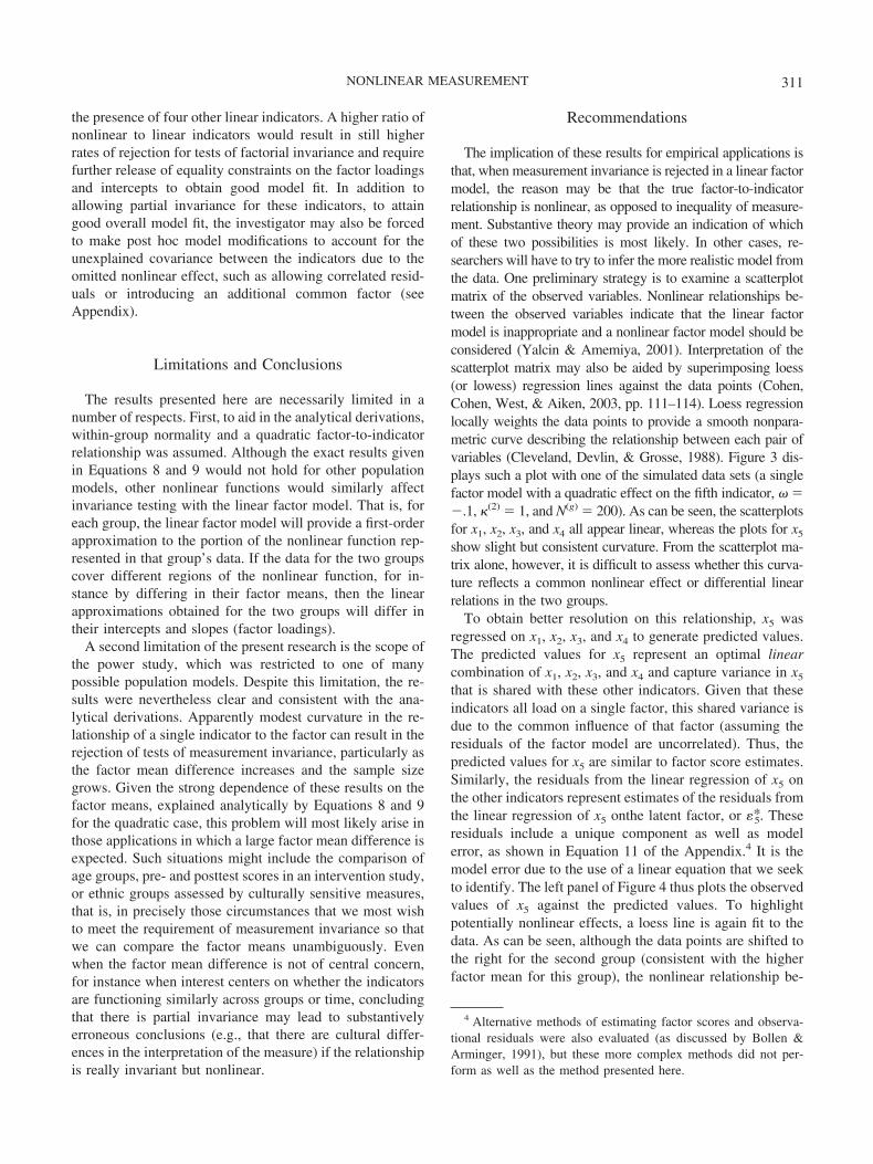
The implication of these results for empirical applications isthat, when measurement invariance is rejected in a linear factormodel, the reason may be that the true factor-to-indicatorrelationship is nonlinear, as opposed to inequality of measure-ment. Substantive theory may provide an indication of whichof these two possibilities is most likely. In other cases, re-searchers will have to try to infer the more realistic model fromthe data. One preliminary strategy is to examine a scatterplotmatrix of the observed variables. Nonlinear relationships be-tween the observed variables indicate that the linear factormodel is inappropriate and a nonlinear factor model should beconsidered (Yalcin & Amemiya, 2001). Interpretation of thescatterplot matrix may also be aided by superimposing loess(or lowess) regression lines against the data points (Cohen,Cohen, West, & Aiken, 2003, pp. 111–114). Loess regressionlocally weights the data points to provide a smooth nonpara-metric curve describing the relationship between each pair ofvariables (Cleveland, Devlin, & Grosse, 1988). Figure 3 dis-plays such a plot with one of the simulated data sets (a singlefactor model with a quadratic effect on the fifth indicator, � ��.1, �(2) � 1, and N(g) � 200). As can be seen, the scatterplotsfor x1, x2, x3, and x4 all appear linear, whereas the plots for x5

show slight but consistent curvature. From the scatterplot ma-trix alone, however, it is difficult to assess whether this curva-ture reflects a common nonlinear effect or differential linearrelations in the two groups.

To obtain better resolution on this relationship, x5 wasregressed on x1, x2, x3, and x4 to generate predicted values.The predicted values for x5 represent an optimal linearcombination of x1, x2, x3, and x4 and capture variance in x5

that is shared with these other indicators. Given that theseindicators all load on a single factor, this shared variance isdue to the common influence of that factor (assuming theresiduals of the factor model are uncorrelated). Thus, thepredicted values for x5 are similar to factor score estimates.Similarly, the residuals from the linear regression of x5 onthe other indicators represent estimates of the residuals fromthe linear regression of x5 onthe latent factor, or �*5. Theseresiduals include a unique component as well as modelerror, as shown in Equation 11 of the Appendix.4 It is themodel error due to the use of a linear equation that we seekto identify. The left panel of Figure 4 thus plots the observedvalues of x5 against the predicted values. To highlightpotentially nonlinear effects, a loess line is again fit to thedata. As can be seen, although the data points are shifted tothe right for the second group (consistent with the higherfactor mean for this group), the nonlinear relationship be-

4 Alternative methods of estimating factor scores and observa-tional residuals were also evaluated (as discussed by Bollen &Arminger, 1991), but these more complex methods did not per-form as well as the method presented here.

311NONLINEAR MEASUREMENT

tween x5 and the other indicators appears to be shared byboth groups. This nonlinear trend is also evident in theright panel of Figure 4, which plots the residuals for x5

versus the predicted values (i.e., removing the linearrelationship). Overall, these procedures correctly identi-fied x5 as the sole nonlinear indicator and hence appear tobe useful in diagnosing potential nonlinear effects in thefactor model.

A more general two-step strategy to diagnosing non-linear effects in a factor model would be as follows. First,produce a scatterplot matrix from all of the indicators ofa single factor, as in Figure 3. On the basis of this matrix,partition the factor indicators into two subsets, one subsetwithin which all indicators appear to be linearly related toone another, and another subset for which the assumptionof linearity is more dubious. Second, regress each indi-cator in the second subset on all of the indicators in the

first subset within a multiple linear regression model.Save the predicted values and residuals from the regres-sion model to produce diagnostic plots such as Figure 4for each questionable indicator. Use these plots to aid injudging whether there is a nonlinear relationship betweenthe indicator and factor or there are linear relationships ineach group with different slopes. In the latter case, alinear factor model with partial invariance may be calledfor. In the former case, however, one must address thenonlinear nature of the relationship. Two options fordoing so can be considered: applying a nonlinear trans-formation to the indicator to make the relationship morelinear, so that the original model structure can be re-tained, or revising the model structure to include thenonlinear effect. If one selects the latter option andproceeds to estimate the nonlinear factor model, it wouldseem most reasonable to select an indicator from the first

Figure 3. Scatterplot matrix and loess regression lines fit to the aggregated data from the twogroups. Note the slight but consistent curvature in the relation of x5 to the other factor indicators.

312 BAUER

subset to serve as the anchor for scaling the latent factor.If there are multiple factors in the model, these proce-dures could be repeated for the indicators of each factorin turn.

Unfortunately, given compelling evidence of nonlin-earity in factor-to-indicator relationships, it has, untilrecently, been relatively difficult to fit a nonlinear factoranalysis model. Following the early contributions of Mc-Donald (1967), Etezadi-Amoli and McDonald (1983),and Mooijaart and Bentler (1986), however, new methodsof estimation for nonlinear structural equation modelshave been developed, including the maximum-likeli-hood-based methods of Klein and Moosbrugger (2000),Klein and Muthen (2003), Lee and Zhu (2002), andYalcin and Amemiya (2001); the method of momentsapproach of Wall and Amemiya (2000); and the Bayesianapproaches of Arminger and Muthen (1998) and Zhu andLee (1999). Of these methods, the approximate maxi-mum-likelihood approach of Klein and Moosbrugger(2000) has been incorporated into the commercial soft-ware program Mplus and can be used with multisamplemodels (Muthen & Muthen, 2004). To my knowledge,this is the only software presently available that permitsthe simultaneous estimation of a nonlinear factor modelin two or more groups. Examples of Mplus input files are

provided at http://dx.doi.org/10.1037/1082-989X.10.3.305.supp showing the specification of a quadratic effectin a factor model fit to the simulated data set shown inFigures 3 and 4. It should be noted, however, that theKlein and Moosbrugger approach in Mplus is limited tothe estimation of quadratic functions (or, in other con-texts, product interaction models), whereas some otherapproaches to nonlinear factor analysis permit the esti-mation of more complex functions (but have not yet beenextended to the analysis of multiple samples). If a morecomplex function is required, it may be necessary toconduct a nonlinear factor analysis in each group inde-pendently and then compare the obtained estimates in amore-or-less ad hoc manner.

Two other issues are also worth considering when estimat-ing nonlinear factor models. First, some methods for fittingnonlinear factor models are more reliant on the assumption ofnormality for the latent factors than others. For these methods,failure to meet the assumption of normality may increase therisk of identifying spurious nonlinear effects (see Marsh, Wen,& Hau, 2004). Second, as in multiple regression analysis(Aiken & West, 1991, chap. 5), grand mean centering mayprove useful for interpretational and computational reasonswhen modeling nonlinear effects.

Figure 4. Plot of raw scores (left) and residuals (right) for indicator x5 against predicted values forx5 obtained from the optimal linear combination of x1, x2, x3, and x4. Data points for the two groupsare distinguished by different symbols (o’s for Group 1 and x’s for Group 2). The line superimposedon each plot is obtained from a loess fit to the aggregated data.

313NONLINEAR MEASUREMENT

References

Aiken, L. S., & West, S. G. (1991). Multiple regression: Testingand interpreting interactions. Newbury Park, CA: Sage.

Arminger, G., & Muthen, B. (1998). A Bayesian approach tononlinear latent variable models using the Gibbs sampler andthe Metropolis-Hastings algorithm. Psychometrika, 63, 271–300.

Benton, T., Hand, D., & Crowder, M. (2004). Two zs are betterthan one. Journal of Applied Statistics, 31, 239–247.

Bollen, K. A. (1989). Structural equations with latent variables.New York: Wiley.

Bollen, K. A., & Arminger, G. (1991). Observational residuals infactor analysis and structural equation models. SociologicalMethodology, 21, 235–262.

Borsboom, D., Mellenbergh, G. J., & van Heerden, J. (2002).Different kinds of DIF: A distinction between absolute andrelative forms of measurement invariance and bias. AppliedPsychological Measurement, 26, 433–450.

Byrne, B. M., Shavelson, R. J., & Muthen, B. (1989). Testing forthe equivalence of factor covariance and mean structures: Theissue of partial measurement invariance. Psychological Bulletin,105, 456–466.

Cheung, G. W., & Rensvold, R. B. (1999). Testing factorialinvariance across groups: a reconceptualization and proposednew method. Journal of Management, 25, 1–27.

Cheung, G. W., & Rensvold, R. B. (2002). Evaluating goodness-of-fit indexes for testing measurement invariance. StructuralEquation Modeling, 9, 233–255.

Cleveland, W. S., Devlin, S. J., & Grosse, E. (1988). Regression bylocal fitting. Journal of Econometrics, 37, 87–114.

Cohen, J. (1988). Statistical power analysis for the behavioralsciences (2nd ed.). Hillsdale, NJ: Erlbaum.

Cohen, J., Cohen, P., West, S. G., & Aiken, L. S. (2003). Appliedmultiple regression/correlation analysis for the behavioral sci-ences (3rd ed.). Mahwah, NJ: Erlbaum.

Etezadi-Amoli, J., & McDonald, R. P. (1983). A second generationnonlinear factor analysis. Psychometrika, 48, 315–342.

Goodman, L. (1960). On the exact variance of products. Journal ofthe American Statistical Association, 64, 708–712.

Hancock, G. R. (2001). Effect size, power, and sample size deter-mination for structured means modeling and MIMIC approachesto between-groups hypothesis testing of means on a single latentconstruct. Psychometrika, 66, 373–388.

Horn, J. L., & McArdle, J. J. (1992). A practical and theoreticalguide to measurement invariance in aging research. Experimen-tal Aging Research, 18, 117–144.

Joreskog, K. G. (1971). Simultaneous factor analysis in severalpopulations. Psychometrika, 36, 409–426.

Joreskog, K. G., & Moustaki, I. (2001). Factor analysis of ordinalvariables: A comparison of three approaches. Multivariate Be-havioral Research, 36, 347–387.

Kaplan, D. (1989). Power of the likelihood ratio test in multiplegroup confirmatory factor analysis under partial measurement

invariance. Educational and Psychological Measurement, 49,579–586.

Kaplan, D. (2000). Structural equation modeling: Foundationsand extensions. Thousand Oaks, CA: Sage.

Klein, A., & Moosbrugger, H. (2000). Maximum likelihood esti-mation of latent interaction effects with the LMS method. Psy-chometrika, 65, 457–474.

Klein, A., & Muthen, B. O. (2003). Quasi maximum likelihoodestimation of structural equation models with multipleinteraction and quadratic effects. Manuscript submitted forpublication.

Kline, R. B. (2005). Principles and practice of structural equationmodeling (2nd ed.). New York: Guilford Press.

Lee, S. Y., & Zhu, H. T. (2002). Maximum likelihood estimationof nonlinear structural equation models. Psychometrika, 67,189–210.

Lubke, G. H., Dolan, C. V., Kelderman, H., & Mellenbergh, G. J.(2003). On the relationship between sources of within- andbetween-group differences and measurement invariance in thecommon factor model. Intelligence, 31, 543–566.

Marsh, H. W., Wen, Z., & Hau, K.-T. (2004). Structural equationmodels of latent interactions: evaluation of alternative estima-tion strategies and indicator construction. Psychological Meth-ods, 9, 275–300.

McDonald, R. P. (1967). Nonlinear factor analysis. PsychometricMonograph Number 15. Richmond, VA: William Byrd Press.

McDonald, R. P., & Ho, M.-H. R. (2002). Principles and practicein reporting structural equation analysis. Psychological Meth-ods, 7, 64–82.

Meade, A. W., & Lautenschlager, G. J. (2004). A Monte-Carlo studyof confirmatory factor analytic tests of measurement equivalence/invariance. Structural Equation Modeling, 11, 60–72.

Meredith, W. (1964). Notes on factorial invariance. Psy-chometrika, 29, 177–185.

Meredith, W. (1993). Measurement invariance, factor analysis andfactorial invariance. Psychometrika, 58, 525–543.

Meredith, W., & Horn, J. (2001). The role of factorial invariancein modeling growth and change. In A. Sayer & L. Collins (Eds.),New methods for the analysis of change (pp. 203–240). Wash-ington, DC: American Psychological Association.

Millsap, R. E. (1998). Group differences in regression intercepts:implications for factorial invariance. Multivariate BehavioralResearch, 33, 403–424.

Millsap, R. E., & Kwok, O.-M. (2004). Evaluating the impact ofpartial factorial invariance on selection in two populations.Psychological Methods, 9, 93–115.

Mislevy, R. J. (1986). Recent developments in the factor analysis ofcategorical variables. Journal of Educational Statistics, 11, 3–31.

Mooijaart, A., & Bentler, P. M. (1986). Random polynomial factoranalysis. In E. Diday, Y. Escoufier, L. Lebart, J. Pages, Y.Schektman, & R. Tomassone (Eds.), Data analysis and infor-matics IV (pp. 241–250). Amsterdam: Elsevier Science.

Muthen, B. (1984). A general structural equation model withdichotomous, ordered categorical, and continuous latent vari-able indicators. Psychometrika, 49, 115–132.

314 BAUER

Muthen, B., & Christoffersson, A. (1981). Simultaneous factoranalysis of dichotomous variables in several populations. Psy-chometrika, 46, 407–419.

Muthen, L. K., & Muthen, B. O. (2004). Mplus user’s guide (3rded.). Los Angeles: Muthen & Muthen.

Ployhart, R. E., & Oswald, F. L. (2004). Applications of mean andcovariance structure analysis: Integrating correlational and experi-mental approaches. Organizational Research Methods, 7, 27–65.

Satorra, A., & Saris, W. E. (1985). The power of the likelihood ratiotest in covariance structure analysis. Psychometrika, 50, 83–90.

Sorbom, D. (1974). A general method for studying differences infactor means and factor structure between groups. British Jour-nal of Mathematical and Statistical Psychology, 27, 229–239.

Steenkamp, J. E. M., & Baumgartner, H. (1998). Assessing mea-surement invariance in cross-national consumer research. Jour-nal of Consumer Research, 25, 78–90.

Vandenberg, R. J., & Lance, C. E. (2000). A review and synthesisof the measurement invariance literature: suggestions, practices,and recommendations for organizational research. Organiza-tional Research Methods, 3, 4–69.

Wall, M. M., & Amemiya, Y. (2000). Estimation for polynomialstructural equations. Journal of the American Statistical Asso-ciation, 95, 929–940.

Wall, M. M., & Amemiya, Y. (in press). A review of nonlinearfactor analysis statistical methods. In R. Cudeck & R. C. Mac-

Callum (Eds.), Factor analysis at 100: Historical developments

and future directions. Mahway, NJ: Erlbaum.Waller, N. G., Tellegen, A., McDonald, R. P., & Lykken, D. T.

(1996). Exploring nonlinear models in personality assessment:Development and preliminary validation of a negative emotion-ality scale. Journal of Personality, 64, 545–576.

Weisstein, E. W. (1999). Normal distribution. MathWorld—A Wol-

fram Web Resource. Retrieved January 1, 2005, from http://mathworld.wolfram.com/NormalDistribution.html

Wherry, R. J., & Gaylord, R. H. (1944). Factor pattern of test itemsand tests as a function of the correlation coefficient: Content,difficulty, and constant error factors. Psychometrika, 9, 237–244.

Widaman, K. F., & Reise, S. P. (1997). Exploring the measure-ment invariance of psychological instruments: applications inthe substance use domain. In K. J. Bryant, M. Windle, & S. G.West (Eds.), The science of prevention: Methodological ad-

vances from alcohol and substance abuse research (pp. 281–324). Washington, DC: American Psychological Association.

Yalcin, I., & Amemiya, Y. (2001). Nonlinear factor analysis as astatistical method. Statistical Science, 16, 275–294.

Zhu, H.-T., & Lee, S.-Y. (1999). Statistical analysis of nonlinearfactor analysis models. British Journal of Mathematical and

Statistical Psychology, 52, 225–242.

Appendix

Derivation of Equation 8

This appendix provides a proof of Equation 8 and some addi-tional results using standard rules of covariance algebra (see Bol-len, 1989, pp. 21–23), the moments of the normal distribution(Weisstein, 1999), and expectations of products of normal distri-butions (Benton, Hand, & Crowder, 2004; Goodman, 1960). Tobegin, let us assume that the true factor-to-indicator relationship is

x � � � �� � ��2 � �. (A1)

In addition, let us make the common assumptions that the latentvariable � is normally distributed with mean � and variance , that� is also normally distributed with mean 0 and variance �, and that� is uncorrelated with �.

Now suppose that the form of the fitted model posits that x islinearly related to � such that

x � �* � �*� � �*. (A2)

Because of the omission of the �2 predictor, the coefficients �* and

�* will differ from � and � from Equation A1. The residuals fromthe regression, �*, will also differ from � and hence the varianceof �*, denoted �*, will differ from �.

The coefficient �* can be solved for by noting that

�* �COV��, x�

VAR����

E��x� E��� E� x�

. (A3)

To solve for �*, let us first substitute for x using Equation A1. Thefirst term in the numerator of Equation A3 then becomes

E��x� � E���� � �� � ��2 � ���

� E��� � ��2 � ��3 � ���

� �E��� � �E��2� � �E��3� � E����

� �� � ���2 � � � ���3 � 3�� � 0

� �� � ��2 � � � ��3 � 3��. (A4)

(Appendix continues)

315NONLINEAR MEASUREMENT

A similar substitution in the second term of the numerator yields

E��� E� x� � E��� E�� � �� � ��2 � ��

� E����� � �E��� � �E��2� � E����

� ��� � �� � ���2 � � � 0�

� �� � ��2 � ��3 � ��. (A5)

Subtracting Equation A5 from Equation A4 and inserting the resultinto Equation A3 gives

�* �� � 2��

� � � 2��, (A6)

as indicated in Equation 8. Here it is important to note that if the factoris scaled by setting the mean to zero, then �* will equal �. As aninteresting aside, this is also the result one would obtain by taking thefirst derivative of Equation A1 with respect to � and evaluating at themean of �, or �. That is, the slope given by Equation A6 is also theslope of the tangent line to the true quadratic function at the mean (seealso Aiken & West, 1991, p. 65).

In a similar way, the coefficient �* can be determined by drawingon the familiar equation for the intercept of a regression line:

�* � E� x� �*E���

� E�� � �� � ��2 � �� �*E���

� � � �E��� � �E��2� � E��� �*E���

� � � �� � ���2 � � � 0 �*�. (A7)

Substituting for �* via Equation A6, Equation A7 can be rewrittenas

�* � � � �� � ���2 � � �� � 2����

� � � �� � ��2 � � �� 2��2

� � � � ��2

� � � �� �2�, (A8)

as also indicated in Equation 8.Interest may also center on the change in the residual variance

as a function of the model misspecification. To determine this, theresiduals �* must be expressed in terms of the original modelparameters. Equations A1 and A2 show that

�* � x ��* � �*��

� �� � �� � ��2 � �� ��* � �*��

� � � ��� � �� � ��2� ��* � �*���. (A9)

The grouping of terms given on the third line of Equation A9 hasthe intuitively pleasing interpretation that the residuals of themisspecified model are equal to the original residuals plus thediscrepancy between the true and fitted regression function. Thatis, the residuals include both random error and model error. Sub-

stituting the results given in Equations A6 and A8 for �* and �*and subsequent simplification then yields

�* � � � � � �� � ��2 �� � �� �2� � �� � 2�����

� � � ���2 2�� � �2�. (A10)

The reader can verify that E(�*) is zero.Using the prior results, and assuming normality of �, the vari-

ance of �*, denoted �*, can be expressed as

�* � E��*2�

� E�� � ���2 2�� � �2��2�

� E��2� 4��E���� 2�E��� � 2�2�E��� � 2�E��2��

� 4��2E��� � �4�2 � 2�2 � �2E��4� 2�2�2

4��2E��3� 4�3�2E��� 2�2E��2� � 6�2�2E��2�

� � � 4��2� � �4�2 � 2�2 � �2��4 � 6�2 � 32�

2�2�2 4��2��3 � 3�� 4�3�2�

2�2��2 � � � 6�2�2��2 � �

� � � 22�2. (A11)

As one would expect, Equation A11 implies that �* � � for allvalues of and �, with the inequality increasing with the degreeof curvature in the true relationship and the degree of dispersion ofthe latent factor. That �* does not depend on the factor mean is aconsequence of the symmetry of the quadratic function: A linearapproximation will perform equally well at all points on thequadratic function. For other nonlinear functions, a linear approx-imation may vary in quality depending on what portion of thenonlinear function is being approximated (i.e., how nonlinear thatportion of the function is). Hence, for other functions, �* may alsodepend on the factor mean.

Using derivations similar to Equation A11, it is also possible toshow that if two indicators, say x1 and x2, are both quadraticallyrelated to the latent factor �, then the covariance of the residualsobtained from fitting a partially invariant linear factor model willequal

COV��*1, �*2� � COV��1, �2� � 22�1�2, (A12)

where the subscripts differentiate the residuals and quadratic ef-fects for the two indicators. If local independence holds in thepopulation and COV(�1, �2) � 0, then this reduces to COV(�*1,�*2) � 22�1�2. It is this apparent common variance unexplainedby the linear factor model that can lead to the estimation ofso-called difficulty factors to obtain good overall model fit. Alter-natively, post hoc model modifications to allow for correlatedresiduals would also produce good model fit, in effect obscuringthe misspecification of the nonlinear factor-to-indicator relation-ships. Note that in the multiple group context, if the factor vari-ances differ between groups (or the quadratic effects), then theresidual covariance will also differ.

Received September 8, 2004Revision received May 24, 2005

Accepted May 27, 2005 �

316 BAUER