The Role of Agricultural and

Non-Agricultural Productivity in Latin

American Development

Carlos Machicado a, Felix Rioja b, Antonio Saravia c,∗,

aInstitute for Advanced Development StudiesbDepartment of Economics, Georgia State University

cDeloitte Tax LLP and Department of Economics, Georgia State University

Abstract

We calibrate a simple neoclassical model of structural transformation for Chile,Brazil, Colombia, Ecuador, Peru, Paraguay and Bolivia. We show that slow growthin agricultural productivity can substantially delay the development process andresult in significant differences in per capita incomes. The development process canbe accelerated, however, by increasing productivity in the non-agricultural sector.In fact, in the long run, it is non-agricultural productivity what determines conver-gence. In our various exercises we find that...

Key words: Economic Development, Latin America, Agriculture Productivity,Manufacturing ProductivityJEL Classification: O47, O57, E13

1 Introduction

According to Lucas (2000), one of the fundamental reasons for the large in-come disparities observed between poor and rich countries is that the formerstarted the process of industrialization much later than the latter. On thisline of thought, Gollin, Parente, and Rogerson (2002) (henceforth GPR (2002))suggest that countries begin the process of industrialization only after they areable to satisfy their basic agricultural (food) needs. According to these authors,

∗ Corresponding author.Email addresses: cmachicado@inesad.edu.bo (Carlos Machicado),

frioja@gsu.edu (Felix Rioja), asaravia@gsu.edu (Antonio Saravia).

Preprint submitted to LACEA 23 May 2011

therefore, improvements in agricultural productivity are key determinants ofdevelopment as they allow countries to reach their basic agricultural needssooner and begin to free up resources for the process of industrialization. Onthe contrary, countries experiencing low agricultural productivity levels wouldtend to lag behind.

In this paper we evaluate the potential of the GPR (2002) model in explain-ing the observed patterns of development in a sample of seven Latin Americancountries including Chile, Brazil, Colombia, Ecuador, Peru, Paraguay, and Bo-livia. Studying a group of countries sharing similar colonial institutions andculture allows us to better evaluate the proposed channels of development de-scribed by the model. We find that our calibrated version of the GPR (2002)model generates paths of development that fit the observed data. Our exerciseclearly illustrates that, while differences in agricultural productivity deter-mine the extent of income differences during the first number of periods, it isnon-agricultural productivity what determines the speed of convergence. Wechoose Chile as our benchmark economy. According to our data, Chile startedto industrialize much earlier than the other countries in our sample. Not sur-prisingly, therefore, In recent periods, Chile’s income per capita has been 40to 80 percent higher than the corresponding figure in the other countries.

The importance of agriculture for the industrialization process has been longnoted in the development literature as in Johnston and Mellor (1961), John-ston and Kilby (1975) and Timmer (1988, 2002). Before industrialization,almost all the labor force worked in agriculture. Once agricultural produc-tivity rises enough to allow the production of subsistence level of food, thenlabor moves out of the agricultural sector and into the non-agricultural sector.Hence, the agricultural sector as a share of the economy and the labor forcestarts falling.

The model by GPR (2002) can be considered an extension of Laitner’s (2000)and Hansen and Prescott’s (2002). The literature on this topic also includes,Caselli and Coleman (2001), who study the role of human capital accumulationas a factor that contributes to how quickly labor can move out of agriculture.Also, in a follow up paper, GPR (2007) use a similar model to account fora feedback effect from the manufacturing sector to agriculture. In a recentpaper, Restuccia, Yang and Zhu (2008) also find that agricultural productivityis important for structural transformation, but that barriers to the adoption ofagricultural technology explain the differences in both agricultural and overallproductivity among countries. These studies are part of a broader branch of theliterature studying agriculture in growth frameworks; for example, Echeverria(1997), Kongsamut et al. (2001), Glomm (1992), and Lucas (2004).

As we mentioned before, our findings indicate that the model provides anadequate description of the observed income disparities of the seven Latin

2

American countries in our sample. Low agricultural productivity delays thebeginning of the process industrialization, in some cases - like Paraguay andBolivia -, by about 100 years compared to the leader of the group, Chile.We also find that the reduction in income differences (convergence) dependscritically on productivity in the non-agricultural sector. Improvements in non-agricultural productivity between 20 and 100 percent would be required tosignificantly close the income gap with Chile by the end of the century.

The paper proceeds as follows. Section 2 describes the model. Section 3 presentsthe calibration and quantitative evaluation. Section 4 concludes.

2 The Model

The basic structure of the GPR (2002) model is that of the one sector neo-classical growth model extended to include an explicit agricultural sector. Inthis framework, development is associated with industrialization. Industrial-ization happens only when the country experiences a structural transformation(namely an improvement on agricultural productivity) that withdraws employ-ment from the agricultural sector and moves it into the non-agricultural sector.Asymptotically, agriculture’s employment share shrinks to zero and the modelbecomes identical to the standard one-sector neoclassical growth model. Wepresent here the basic features of the model.

2.1 Representative household

The econonmy is inhabited by an infinitely-lived household, endowed with aunit of time in each period, who maximizes lifetime utility as given by:

∞∑t=0

βtU(ct, at) (1)

where ct is the non-agricultural good and at is the agricultural good.

GPR (2002) adopt a Stone-Geary variety for the functional form of the utilityfunction in order to generate a structural transformation.

U(ct, at) =

log(ct) + a if at ≥ a

at if at < a(2)

3

This extreme functional form allows the economy to withdraw labor from theagricutural sector once (per capita) output in this sector reaches the subsis-tence level of a. There is nothing particularly special about the value of aand the results are not be much affected if it was either somewhat higher orlower. 1

2.2 Nonagricultural sector

GPR (2002) correctly called one of the sectors of this economy the “non-agricultural” sector, since it includes not only manufacturing but also services,industrial agriculture, and everything else. This sector produces output (Ymt)by combining capital (Kmt) and labor (Nmt) using the following function:

Ymt = Am[Kθmt((1 + γm)tNmt)

1−θ + αNmt

](3)

where Am (TFP) is assumed country-specific and determined by policies andinstitutions. The rate of exogenous technological change (γm) and the (small)number α are assumed identical across countries. Since developing countriesare generally not in the business of creating ideas, the assumption of exogenoustechnological change is reasonable from their perspective. 2

The law of motion for the stock of capital is standard:

Kmt+1 = (1− δ)Kmt +Xmt (4)

where δ is the depreciation rate and Xmt is investment. In fact, output fromthe non-agricultural sector can be used for consumption or investment.

2.3 Agricultural sector

The agricultural sector produces output (Yat) using only labor (Nat). There aretwo available technologies for producing the agricultural good: a traditionaland a modern one. 3

In the traditional technology, one unit of time produces a units of the agricul-tural good. GPR (2002) point out that there are theoretical reasons to believe

1 An expanded version of this model is found in Gollin et.al. (2004) where the stateof the non-agricultural sector can determine the labor allocated to agriculture.2 This could arguably be a strong assumption for countries like Chile and Brazil.3 Adding land as a factor of production would have no impact on the results.

4

that a value close to a is appropriate. Models with endogenous fertility, forexample, suggest that output per capita will be close to subsistence levels foreconomies that have not begun the process of industrialization. 4

On the other hand, the modern agricultural technology is subject to exogenoustechnological change:

Yat = Aa(1 + γa)tNat (5)

where Aa (TFP) is assumed country-specific and determined by policies andinstitutions. It is also affected by climate conditions and the quantity andquality of land per person. Technological innovations that are useful for aspecific crop in a given climate may not be particularly relevant for othercrops in other parts of the world. This effect may generate large differences incross-country productivity levels that are independent of policy.

GPR (2002) assume that the rate of exogenous technological change, γa, iscommon across countries and output from this sector is only used for con-sumption. Therefore, the agriculture resource constraint is simply:

at ≤ Yat (6)

It is important to mention that the agricultural sector is a “basic” agriculturalsector in the sense that its output only satisfy “basic needs.” So, this agri-cultural sector needs to be clearly differentiated from industrial agriculture oragriculture for export.

2.4 The competitive equilibrium

Here we briefly describe the competitive equilibrium of this economy by fo-cusing on how different values of agricultural TFP (Aa) affect the resultingdynamic allocations. The competitive equilibrium involves two steps:

(1) At the beginning labor is allocated entirely to agriculture until:

Aa(1 + γa)t ≥ a

Once this is satisfied, agricultural production switches to the moderntechnology and labor starts to flow out of agriculture at the rate γa.

4 See Oded Galor and David Weil (2000) and Hansen and Prescott (2002).

5

Hence:

Nat = min

{a

Aa(1 + γa)t, 1

}and

Nmt = 1−Nat

(2) Given the time path of labor allocations, the optimal path of investmentis found by solving the households’ optimization problem. Householdschoose consumption of the non-agricultural good and capital to maximizethe utility function (1) subject to the feasibility constraint:

ct +Xmt = Ymt

and the law of motion of capital (equation 4). 5

The Euler equation for this optimization problem is:

Am[Kmt+1θ((1 + γm)t+1Nmt+1)1−θ + αNmt+1]−Kmt+2 + (1− δ)Kmt+1

βAm[Kmtθ((1 + γm)tNmt)1−θ + αNmt]−Kmt+1 + (1− δ)Kmt

= AmKmt+1θ−1θ((1 + γm)t+1Nmt+1)1−θ + 1− δ

and the steady state capital level is:

Kmss =

[(1/β − 1 + δ)

(Am)θ((1 + γm)ssNmss)1−θ

]1/(θ−1)

(7)

This is equivalent to solving the transitional dynamics of the neoclassicalgrowth model with an exogenous time profile of labor input given by Nmt.As technology in the agriculture sector increases at rate γa, Nat eventuallyapproaches 0, and Nmt approaches 1. Asymptotically, therefore, the model isidentical to the standard one-sector neoclassical growth model.

3 Empirical Exercises

In this section we show that differences in agricultural and non-agriculturalproductivity explain the observed differences in incomes per-capita in oursample of seven Latin American countries. We perform some numerical simu-lations to show the usefulness of the model in providing quantitative analysisand policy implications.

Before describing the data and the calibration, it is important to show theevolution of GDP per capita for the countries in our sample. Our data rangesfrom 1900 to 2000.

5 and the appropriate nonnegativity constraints and constraints on Kmt.

6

0

0.2

0.4

0.6

0.8

1

1.2

1.4

1.6

1.8

1900 1910 1920 1930 1940 1950 1960 1970 1980 1990 2000

GDPpercapita(thousandconstant1970PPP$)

Chile

Brazil

Bolivia

Colombia

Peru

Ecuador

Paraguay

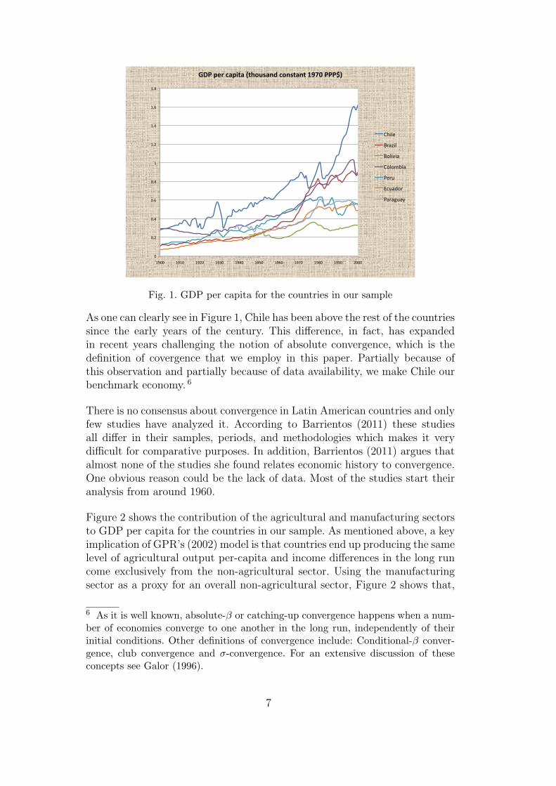
Fig. 1. GDP per capita for the countries in our sample

As one can clearly see in Figure 1, Chile has been above the rest of the countriessince the early years of the century. This difference, in fact, has expandedin recent years challenging the notion of absolute convergence, which is thedefinition of covergence that we employ in this paper. Partially because ofthis observation and partially because of data availability, we make Chile ourbenchmark economy. 6

There is no consensus about convergence in Latin American countries and onlyfew studies have analyzed it. According to Barrientos (2011) these studiesall differ in their samples, periods, and methodologies which makes it verydifficult for comparative purposes. In addition, Barrientos (2011) argues thatalmost none of the studies she found relates economic history to convergence.One obvious reason could be the lack of data. Most of the studies start theiranalysis from around 1960.

Figure 2 shows the contribution of the agricultural and manufacturing sectorsto GDP per capita for the countries in our sample. As mentioned above, a keyimplication of GPR’s (2002) model is that countries end up producing the samelevel of agricultural output per-capita and income differences in the long runcome exclusively from the non-agricultural sector. Using the manufacturingsector as a proxy for an overall non-agricultural sector, Figure 2 shows that,

6 As it is well known, absolute-β or catching-up convergence happens when a num-ber of economies converge to one another in the long run, independently of theirinitial conditions. Other definitions of convergence include: Conditional-β conver-gence, club convergence and σ-convergence. For an extensive discussion of theseconcepts see Galor (1996).

7

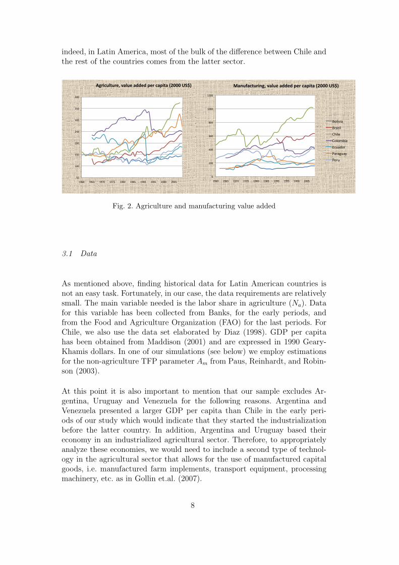
indeed, in Latin America, most of the bulk of the difference between Chile andthe rest of the countries comes from the latter sector.

50

100

150

200

250

300

350

400

1960 1965 1970 1975 1980 1985 1990 1995 2000 2005

Agriculture,valueaddedpercapita(2000US$)

Bolivia

Brazil

Chile

Colombia

Ecuador

Paraguay

Peru

0

200

400

600

800

1000

1200

1960 1965 1970 1975 1980 1985 1990 1995 2000 2005

Manufacturing,valueaddedpercapita(2000US$)

Bolivia

Brazil

Chile

Colombia

Ecuador

Paraguay

Peru

Fig. 2. Agriculture and manufacturing value added

3.1 Data

As mentioned above, finding historical data for Latin American countries isnot an easy task. Fortunately, in our case, the data requirements are relativelysmall. The main variable needed is the labor share in agriculture (Na). Datafor this variable has been collected from Banks, for the early periods, andfrom the Food and Agriculture Organization (FAO) for the last periods. ForChile, we also use the data set elaborated by Diaz (1998). GDP per capitahas been obtained from Maddison (2001) and are expressed in 1990 Geary-Khamis dollars. In one of our simulations (see below) we employ estimationsfor the non-agriculture TFP parameter Am from Paus, Reinhardt, and Robin-son (2003).

At this point it is also important to mention that our sample excludes Ar-gentina, Uruguay and Venezuela for the following reasons. Argentina andVenezuela presented a larger GDP per capita than Chile in the early peri-ods of our study which would indicate that they started the industrializationbefore the latter country. In addition, Argentina and Uruguay based theireconomy in an industrialized agricultural sector. Therefore, to appropriatelyanalyze these economies, we would need to include a second type of technol-ogy in the agricultural sector that allows for the use of manufactured capitalgoods, i.e. manufactured farm implements, transport equipment, processingmachinery, etc. as in Gollin et.al. (2007).

8

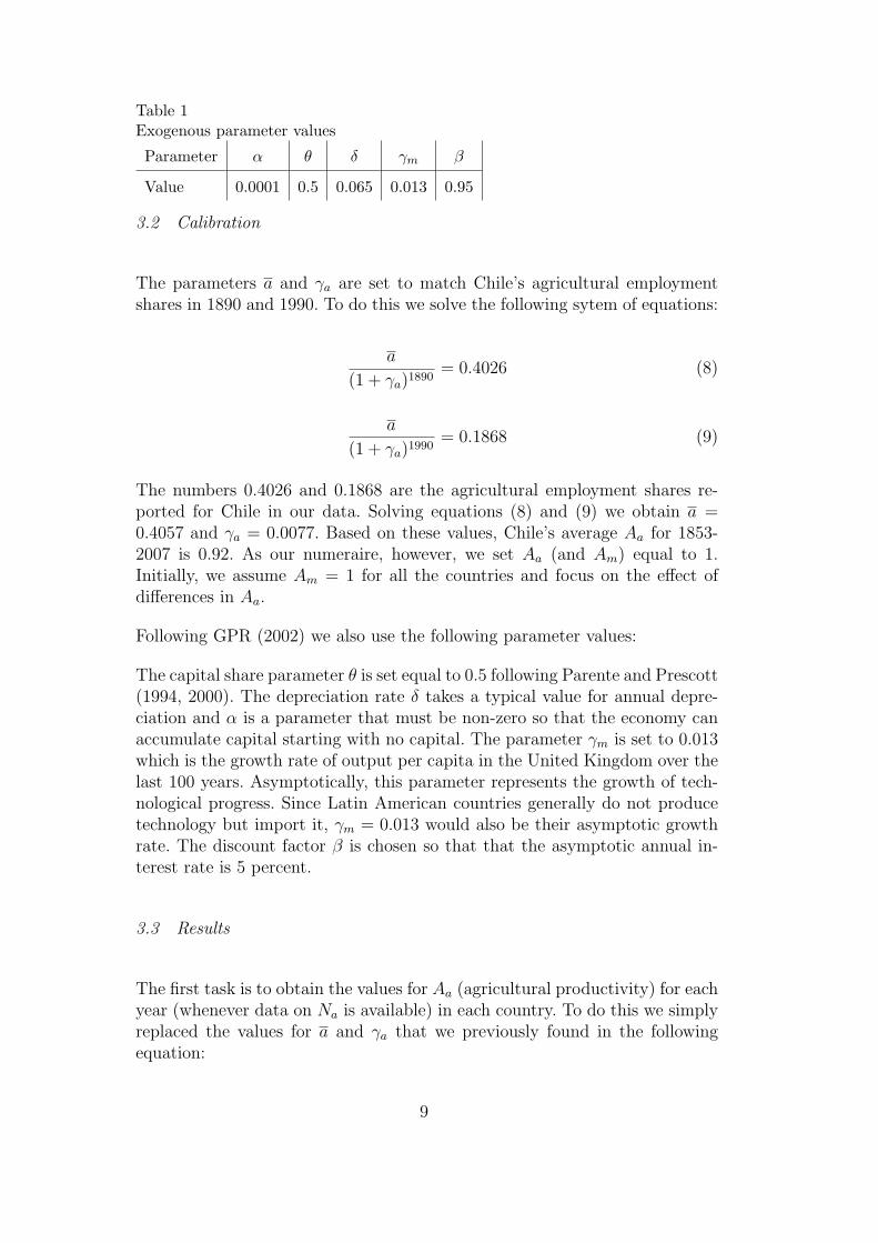
Table 1Exogenous parameter values

Parameter α θ δ γm β

Value 0.0001 0.5 0.065 0.013 0.95

3.2 Calibration

The parameters a and γa are set to match Chile’s agricultural employmentshares in 1890 and 1990. To do this we solve the following sytem of equations:

a

(1 + γa)1890= 0.4026 (8)

a

(1 + γa)1990= 0.1868 (9)

The numbers 0.4026 and 0.1868 are the agricultural employment shares re-ported for Chile in our data. Solving equations (8) and (9) we obtain a =0.4057 and γa = 0.0077. Based on these values, Chile’s average Aa for 1853-2007 is 0.92. As our numeraire, however, we set Aa (and Am) equal to 1.Initially, we assume Am = 1 for all the countries and focus on the effect ofdifferences in Aa.

Following GPR (2002) we also use the following parameter values:

The capital share parameter θ is set equal to 0.5 following Parente and Prescott(1994, 2000). The depreciation rate δ takes a typical value for annual depre-ciation and α is a parameter that must be non-zero so that the economy canaccumulate capital starting with no capital. The parameter γm is set to 0.013which is the growth rate of output per capita in the United Kingdom over thelast 100 years. Asymptotically, this parameter represents the growth of tech-nological progress. Since Latin American countries generally do not producetechnology but import it, γm = 0.013 would also be their asymptotic growthrate. The discount factor β is chosen so that that the asymptotic annual in-terest rate is 5 percent.

3.3 Results

The first task is to obtain the values for Aa (agricultural productivity) for eachyear (whenever data on Na is available) in each country. To do this we simplyreplaced the values for a and γa that we previously found in the followingequation:

9

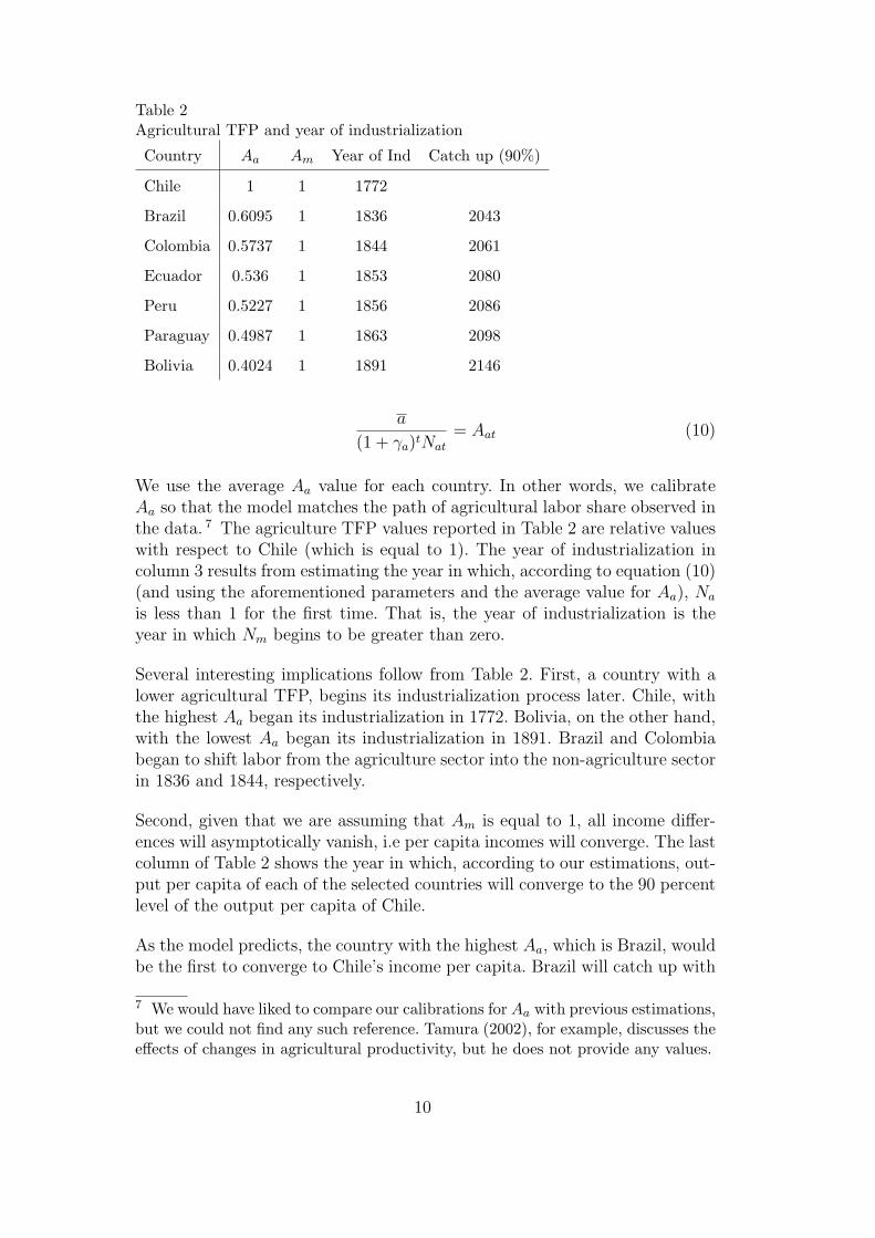
Table 2Agricultural TFP and year of industrialization

Country Aa Am Year of Ind Catch up (90%)

Chile 1 1 1772

Brazil 0.6095 1 1836 2043

Colombia 0.5737 1 1844 2061

Ecuador 0.536 1 1853 2080

Peru 0.5227 1 1856 2086

Paraguay 0.4987 1 1863 2098

Bolivia 0.4024 1 1891 2146

a

(1 + γa)tNat

= Aat (10)

We use the average Aa value for each country. In other words, we calibrateAa so that the model matches the path of agricultural labor share observed inthe data. 7 The agriculture TFP values reported in Table 2 are relative valueswith respect to Chile (which is equal to 1). The year of industrialization incolumn 3 results from estimating the year in which, according to equation (10)(and using the aforementioned parameters and the average value for Aa), Na

is less than 1 for the first time. That is, the year of industrialization is theyear in which Nm begins to be greater than zero.

Several interesting implications follow from Table 2. First, a country with alower agricultural TFP, begins its industrialization process later. Chile, withthe highest Aa began its industrialization in 1772. Bolivia, on the other hand,with the lowest Aa began its industrialization in 1891. Brazil and Colombiabegan to shift labor from the agriculture sector into the non-agriculture sectorin 1836 and 1844, respectively.

Second, given that we are assuming that Am is equal to 1, all income differ-ences will asymptotically vanish, i.e per capita incomes will converge. The lastcolumn of Table 2 shows the year in which, according to our estimations, out-put per capita of each of the selected countries will converge to the 90 percentlevel of the output per capita of Chile.

As the model predicts, the country with the highest Aa, which is Brazil, wouldbe the first to converge to Chile’s income per capita. Brazil will catch up with

7 We would have liked to compare our calibrations for Aa with previous estimations,but we could not find any such reference. Tamura (2002), for example, discusses theeffects of changes in agricultural productivity, but he does not provide any values.

10

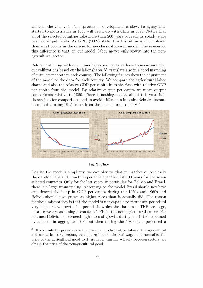
Chile in the year 2043. The process of development is slow. Paraguay thatstarted to industrialize in 1863 will catch up with Chile in 2098. Notice thatall of the selected countries take more than 200 years to reach its steady-staterelative output levels. As GPR (2002) state, this transition is much slowerthan what occurs in the one-sector neoclassical growth model. The reason forthis difference is that, in our model, labor moves only slowly into the non-agricultural sector.

Before continuing with our numerical experiments we have to make sure thatour calibrations based on the labor shares Na translate also in a good matchingof output per capita in each country. The following figures show the adjustmentof the model to the data for each country. We compare the agricultural laborshares and also the relative GDP per capita from the data with relative GDPper capita from the model. By relative output per capita we mean outputcomparisons relative to 1950. There is nothing special about this year, it ischosen just for comparisons and to avoid differences in scale. Relative incomeis computed using 1995 prices from the benchmark economy. 8

0

0.2

0.4

0.6

0.8

1

1.2

1771 1821 1871 1921 1971 2021 2071 2121 2171 2221 2271

Chile:AgriculturalLaborShare

Model

Data

0

0.5

1

1.5

2

2.5

3

1900 1910 1920 1930 1940 1950 1960 1970 1980 1990 2000

Chile:GDPpcRela/veto1950

Model

Data

Fig. 3. Chile

Despite the model’s simplicity, we can observe that it matches quite closelythe development and growth experience over the last 100 years for the sevenselected countries. Only for the last years, in particular for Bolivia and Brazil,there is a large mismatching. According to the model Brazil should not haveexperienced the jump in GDP per capita during the 1950s and 1960s andBolivia should have grown at higher rates than it actually did. The reasonfor these mismatches is that the model is not capable to reproduce periods ofvery high or low growth, i.e. periods in which the changes in TFP are large,because we are assuming a constant TFP in the non-agricultural sector. Forinstance Bolivia experienced high rates of growth during the 1970s explainedby a boost in aggregate TFP, but then during the 1980s it experienced a

8 To compute the prices we use the marginal productivity of labor of the agriculturaland nonagricultural sectors, we equalize both to the real wages and normalize theprice of the agricultural good to 1. As labor can move freely between sectors, weobtain the price of the nonagricultural good.

11

0

0.2

0.4

0.6

0.8

1

1.2

1843 1893 1943 1993 2043 2093 2143 2193 2243 2293

Colombia:AgriculturalLaborShare

Model

Data

0

0.5

1

1.5

2

2.5

3

3.5

4

1900 1910 1920 1930 1940 1950 1960 1970 1980 1990 2000

Colombia:GDPpcRela1veto1950

Model

Data

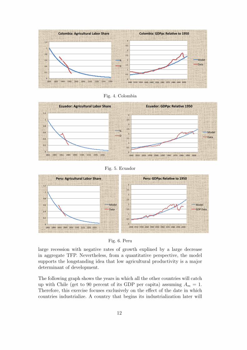
Fig. 4. Colombia

0

0.2

0.4

0.6

0.8

1

1.2

1855 1905 1955 2005 2055 2105 2155 2205 2255

Ecuador:AgriculturalLaborShare

Model

Data

0

0.5

1

1.5

2

2.5

3

3.5

4

1900 1910 1920 1930 1940 1950 1960 1970 1980 1990 2000

Ecuador:GDPpcRela1ve1950

Model

Data

Fig. 5. Ecuador

0

0.2

0.4

0.6

0.8

1

1.2

1855 1905 1955 2005 2055 2105 2155 2205 2255

Peru:AgriculturalLaborShare

Model

Data

0

0.5

1

1.5

2

2.5

3

3.5

4

1900 1910 1920 1930 1940 1950 1960 1970 1980 1990 2000

Peru:GDPpcRela.veto1950

Model

GDPData

Fig. 6. Peru

large recession with negative rates of growth explined by a large decreasein aggregate TFP. Nevertheless, from a quantitative perspective, the modelsupports the longstanding idea that low agricultural productivity is a majordeterminant of development.

The following graph shows the years in which all the other countries will catchup with Chile (get to 90 percent of its GDP per capita) assuming Am = 1.Therefore, this exercise focuses exclusively on the effect of the date in whichcountries industrialize. A country that begins its industrialization later will

12

0

0.2

0.4

0.6

0.8

1

1.2

1862 1912 1962 2012 2062 2112 2162 2212 2262

Paraguay:AgriculturalLaborShare

Model

Data

0

0.5

1

1.5

2

2.5

3

3.5

4

1900 1910 1920 1930 1940 1950 1960 1970 1980 1990 2000

Paraguay:GDPpcRela0veto1950

Model

Data

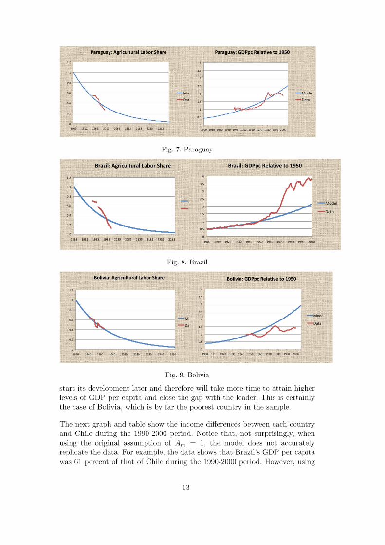
Fig. 7. Paraguay

0

0.2

0.4

0.6

0.8

1

1.2

1835 1885 1935 1985 2035 2085 2135 2185 2235 2285

Brazil:AgriculturalLaborShare

Model

Data

0

0.5

1

1.5

2

2.5

3

3.5

4

1900 1910 1920 1930 1940 1950 1960 1970 1980 1990 2000

Brazil:GDPpcRela0veto1950

Model

Data

Fig. 8. Brazil

0

0.2

0.4

0.6

0.8

1

1.2

1890 1940 1990 2040 2090 2140 2190 2240 2290

Bolivia:AgriculturalLaborShare

Model

Data

0

0.5

1

1.5

2

2.5

3

3.5

4

1900 1910 1920 1930 1940 1950 1960 1970 1980 1990 2000

Bolivia:GDPpcRela0veto1950

Model

Data

Fig. 9. Bolivia

start its development later and therefore will take more time to attain higherlevels of GDP per capita and close the gap with the leader. This is certainlythe case of Bolivia, which is by far the poorest country in the sample.

The next graph and table show the income differences between each countryand Chile during the 1990-2000 period. Notice that, not surprisingly, whenusing the original assumption of Am = 1, the model does not accuratelyreplicate the data. For example, the data shows that Brazil’s GDP per capitawas 61 percent of that of Chile during the 1990-2000 period. However, using

13

0.3

0.4

0.5

0.6

0.7

0.8

0.9

1

1771 1801 1831 1861 1891 1921 1951 1981 2011 2041 2071 2101 2131 2161 2191 2221 2251 2281

GDPpcRela+vetoChile

Brazil

Bolivia

Colombia

Peru

Ecuador

Paraguay

Fig. 10. Paths

0.3

0.4

0.5

0.6

0.7

0.8

0.9

1

1771 1801 1831 1861 1891 1921 1951 1981 2011 2041 2071 2101 2131 2161 2191 2221 2251 2281

GDPpcRela+vetoChile

Brazil

Bolivia

Colombia

Peru

Ecuador

Paraguay

Fig. 11. Catch up

Am = 1 for Brazil, the model predicts that number to be 85 percent. If weuse the manufacturing productivity values reported by Paus, Reinhardt, andRobinson (2003), however, the model predicts exactly 61 percent.

Unfortunately, values for Am were only available for Brazil, Colombia, andPeru. For Ecuador, Paraguay and Bolivia, we estimate the values that wouldgenerate the best fit of the data. These values are reported in column 5 ofTable 3.

14

Table 3Relative income in 1990-2000 with different values of non-agricultural TFP

Country Data M (Am = 1) M (actual Am) Actual Am

Brazil 0.6187 0.8507 0.6141 0.8289

Colombia 0.6762 0.8267 0.6231 0.8503

Ecuador 0.3779 0.7977 0.3766 0.63

Peru 0.3694 0.7865 0.345 0.5975

Paraguay 0.4175 0.7647 0.415 0.69

Bolivia 0.224 0.6502 0.2119 0.45

Table 4Percentage change of non-agricultural TFP to catch up with Chile in 2100

Country Aa Current Am Needed Am Dif

Brazil 0.6095 0.8289 0.98 18.23%

Colombia 0.5737 0.8503 0.99 16.42%

Ecuador 0.536 0.63 0.993 57.62%

Peru 0.5227 0.5975 0.994 66.34%

Paraguay 0.4987 0.69 1 44.93%

Bolivia 0.4024 0.45 1.03 128.89%

Finally, a typical question in the growth literature, in particular when weare interested in absolute convergence, is: How long would it take a countryto close its GDP per capita gap with the leader? Here we slightly modifythe question and ask: By how much should the non-agricultural TFP (Am)increase in each country in order to catch up with Chile by the end of thiscentury? In other words we simulate the value of Am that would allow eachcountry to catch up with Chile in 2100. The results are reported in Table 4.

Brazil, which is the country closer to Chile, will need Am = 0.98 to catch upwith it (get to the 90% of Chiles per capita GDP). That represents an 18.23percent increase in non-agricultural productivity. The same variable will haveto increase by 16.42 percent in Colombia to catch up with Chile in 2100. InBolivia, productivity in sectors like hydrocarbons, mining, manufacturing andothers would need to increase by 129 percent, if Bolivia aims to converge toChile in 2100.

15

4 Concluding Remarks

Using a simple model developed by GPR (2002) we show that differencesin agricultural and non-agricultural productivity can explain differences inincome per capita among a sub-sample of Latin American countries. We per-form several exercises comparing the development paths of Brazil, Colombia,Ecuador, Peru, Paraguay and Bolivia with the development path of Chile, ourbenchmark economy. The model generates series of output per capita (relativeto 1950) very similar to the ones displayed using Maddison’s (2001) data.

The basic structure of the GPR (2002) model is that of the one sector neo-classical growth model extended to include an explicit agricultural sector. Inthis framework, development is associated with industrialization. Industrial-ization happens only when the country experiences a structural transformation(namely an improvement on agricultural productivity) that withdraws employ-ment from the agricultural sector and moves it into the non-agricultural sector.Asymptotically, agricultures employment share shrinks to zero and the modelbecomes identical to the standard one-sector neoclassical growth model.

The results show that, according to our calibration, Chile started its industri-alization process in 1772, Brazil in 1836, Colombia in 1844, Ecuador in 1853,Peru in 1856, Paraguay in 1863 and Bolivia in 1891. Assuming the same level ofnon-agricultural productivity for all the economies, these countries will catchup with Chile in 2043, 2061, 2080, 2086, 2098, and 2146 respectively.

If we abandon the assumption of equal levels of non-agricultural productivityand, instead, we use the much lower values reported by Paus, Reinhardt, andRobinson (2003), we show that, for example, Brazil would have to increaseits non-agricultural TFP by 18.2 percent in order to catch up with Chile in2100. The poorest country, Bolivia, in turn, would need to increase its non-agricultural TFP by 129 percent if it aims to catch up with Chile in the sameyear.

Our research agenda includes the use of the model to study the effect ofinstitutional changes in agriculture that could increase or decrease agriculturalproductivity (e.g. agrarian reforms).

5 References

Barrientos, Paola. 2011. Convergence Clubs in Latin America: A HistoricalApproach. Unpublished manuscript, School of Economics and Management,University of Arhus, Denmark.

16

Caselli, F. and W.J. Coleman II, 2001. The US structural transformation andregional convergence: a reinterpretation. Journal of Political Economy 109 (3),584–616.

Caselli, F. 2005. Accounting for Cross-Country Income Differences. Chapter 9in Handbook of Economic Growth, P. Aghion and S. Durlauf, editors. Elsevier.

Dıaz Jose, Rolf Luders y Gert Wagner.1998. Economıa Chilena 1810-1995:Evolucion Cuantitativa del Producto Total y Sectorial, Documento de TrabajoNo. 186, PUC-Chile.

Echevarria, C., 1997. Changes in sectoral composition associated with eco-nomic growth. International Economic Review 38 (2), 431–452.

Galor, Oded. 1996. Convergence? Inferences from theoretical models. The Eco-nomic Journal, Vol. 106, No. 437, pp. 1056-1069.

Galor, Oded and David Weil. 2000. Population, Technology, and Growth: FromMalthusian Stagnation to the Demographic Transition and Beyond. AmericanEconomic Review, 90(4), pp: 806-828.

Glomm, G., 1992. A model of growth and migration. Canadian Journal ofEconomics 42 (4), 901–922.

Gollin, D. 2002. Getting Income Shares Right. Journal of Political Economy,Vol. 110 (2), pp. 458-474..

Gollin, Douglas, Stephen Parente, and Richard Rogerson. 2002. The Role ofAgriculture in Development, AEA Papers and Proceedings Vol. 92, No.2, pp:160-164.

Gollin, Douglas, Stephen Parente, and Richard Rogerson. 2004. Farmwork,Homework, and International Productivity Differences. Review of EconomicDynamics, Vol. 7, pp. 827-850.

Gollin, Douglas, Stephen Parente, and Richard Rogerson. 2007. The FoodProblem and the Evolution of International Income Levels. Journal of Mone-tary Economics, Vol. 54 (4), pp. 1230-1255.

Hansen, G., Prescott, E.C., 2002. Malthus to Solow. American Economic Re-view 92 (4), 1205–1217.

Johnston, Bruce F. and John W. Mellor. 1961. The role of agriculture ineconomic development. American Economic Review 51(4): 566-93.

Johnston, Bruce F. and Peter Kilby. 1975. Agriculture and Structural Trans-formation: Economic Strategies in Late-Developing Countries. New York: Ox-

17

ford University Press.

Kongsamut, P., Rebelo, S., Xie, D., 2001. Beyond balanced growth. Review ofEconomic Studies 68 (4), 869–882.

Laitner, J., 2000. Structural change and economic growth. Review of EconomicStudies 67 (July), 545–561.

Lucas Jr., R.E., 2000. Some Macroeconomics for the 21st Century. The Journalof Economic Perspectives, Vol. 14, No. 1. (Winter), pp. 159-168.

Lucas Jr., R.E., 2004. Life earnings and rural–urban Migration. Journal ofPolitical Economy 112 (1, part 2), S29–S59.

Maddison, Angus. 2001). The World Economy: A Millennial Perspec-tive, OECD.

Paus, Eva., Nola Reinhardt, and Michael Robinson. 2003. Trade Liberalizationand Productivity Gorwth in Latin American Manufacturing, 1970-98. PolicyReform, Vol 6(1), pp. 1-15.

Restuccia, Diego, Dennis T. Yang and Xiaodong Zhu. ”Agriculture and Aggre-gate Productivity: A Quantitative Cross-Country Analysis,” Journal of Mon-etary Economics, Volume 55 (2), March 2008, pp. 234-50.

Tamura, Robert (2002). Human capital and the switch from agriculture toindustry, Journal of Economic, Dynamics and Control, 27, pp. 207-242.

Timmer, C. Peter. 1988. The agricultural transformation. Chapter 8 in Hand-book of Development Economics, Vol. I, ed. H. Chenery and T.N. Srinivasan.Amsterdam: Elsevier Science Publishers.

Timmer, C. Peter. 2002. Agriculture and economic development. Chapter 29in Handbook of Agricultural Economics, Vol. 2A: Agriculture and Its ExternalLinkages, ed. Bruce L. Gardner and Gordon C. Rausser. Amsterdam: ElsevierScience Publishers.

18