DI

SC

US

SI

ON

P

AP

ER

S

ER

IE

S

Forschungsinstitut zur Zukunft der ArbeitInstitute for the Study of Labor

The Rise in Absenteeism:Disentangling the Impacts of Cohort, Age and Time

IZA DP No. 5091

July 2010

Erik BiørnSimen GaureSimen MarkussenKnut Røed

The Rise in Absenteeism: Disentangling the Impacts of

Cohort, Age and Time

Erik Biørn University of Oslo

Simen Gaure

Ragnar Frisch Centre for Economic Research

Simen Markussen Ragnar Frisch Centre for Economic Research

Knut Røed

Ragnar Frisch Centre for Economic Research and IZA

Discussion Paper No. 5091 July 2010

IZA

P.O. Box 7240 53072 Bonn

Germany

Phone: +49-228-3894-0 Fax: +49-228-3894-180

E-mail: iza@iza.org

Any opinions expressed here are those of the author(s) and not those of IZA. Research published in this series may include views on policy, but the institute itself takes no institutional policy positions. The Institute for the Study of Labor (IZA) in Bonn is a local and virtual international research center and a place of communication between science, politics and business. IZA is an independent nonprofit organization supported by Deutsche Post Foundation. The center is associated with the University of Bonn and offers a stimulating research environment through its international network, workshops and conferences, data service, project support, research visits and doctoral program. IZA engages in (i) original and internationally competitive research in all fields of labor economics, (ii) development of policy concepts, and (iii) dissemination of research results and concepts to the interested public. IZA Discussion Papers often represent preliminary work and are circulated to encourage discussion. Citation of such a paper should account for its provisional character. A revised version may be available directly from the author.

IZA Discussion Paper No. 5091 July 2010

ABSTRACT

The Rise in Absenteeism: Disentangling the Impacts of Cohort, Age and Time*

We examine the remarkable rise in absenteeism among Norwegian employees since the early 1990’s, with particular emphasis on disentangling the roles of cohort, age, and time. Based on a fixed effects model, we show that individual age-adjusted absence propensities have risen even more than aggregate absence rates from 1993 to 2005, debunking the popular hypothesis that the rise in absenteeism resulted from the inclusion of new cohorts – with weaker work-norms – into the workforce. We also reject the idea that the rise in absenteeism resulted from more successful integration of workers with poor health; on the contrary, a massive rise in disability rolls during the 1990’s suggest that poor-health workers have left the labor market in unprecedented numbers. JEL Classification: C23, C25, I38, J22 Keywords: sickness absence, endogenous selection, multicollinearity, fixed effects logit Corresponding author: Knut Røed Ragnar Frisch Centre for Economic Research Gaustadalléen 21 0349 Oslo Norway E-mail: knut.roed@frisch.uio.no

* This paper is part of the project “Absenteeism in Norway - Causes, Consequences, and Policy Implications”, financed by the Norwegian Research Council (grant #187924).

3

1. Introduction

During the last two decades, the rate at which Norwegian workers are absent from work

due to sickness has risen sharply; from around 4-5 percent of paid hours in the early

1990s to around 6.5 percent today (2010). The rise in absenteeism has occurred despite

general improvements in self-reported health conditions. According to Statistics Nor-

way’s level-of-living surveys, the proportion of the population reporting poor or very

poor health has declined from 10 per cent in 1995 to 8 per cent in 2005 among citizens

above 45 years, while it has remained stable at 3 per cent among younger citizens. Based

on a sample survey on self-reported health complaints and actual absence behavior in

1996 and 2003, Ihlebaek et al. (2007) found that while the prevalence of health com-

plaints remained stable, sickness absence rose by 65 percent.

Why has absenteeism risen so much? Generous sickness insurance – with a 100

percent replacement ratio for up to one year – can potentially explain why Norwegian

absence rates are high; but without a theory of gradual adjustment of behavior in re-

sponse to welfare state generosity (Lindbeck, 1995; Lindbeck et al., 1999), it cannot ex-

plain why they are rising. Today’s sickness insurance system, introduced in 1978, has

undergone no improvements in coverage or generosity over the last decades. Alternative

explanations abound, ranging from deteriorating work-norms or tougher work-

environments, to the inclusion of marginal (and less healthy) individuals in the work-

force. The latter explanation is of particular interest in a Norwegian context, since raising

marginal workers’ employment propensities – together with curbing absenteeism – has

been among the key goals of a tripartite “inclusive workplace agreement” between the

government and the national confederations of employers and employees. If the rise in

absenteeism resulted directly from the integration of marginal workers (who otherwise

4

could have claimed disability benefits) policy makers would view it as a sign of success –

not of failure.

The purpose of the present paper is to explore the empirical relevance of the vari-

ous explanations with a focus on disentangling cohort, age and time effects. Our empiri-

cal basis is individual register data on long-term absence spells (exceeding two weeks)

for virtually all workers in Norway over a 13 year period (1993-2005). The data consti-

tute a large unbalanced panel data set, with entry and exit of workers over time. While

the processes generating labor market entries and exits are of substantial interest in their

own right, they also represent a major problem when attempting to disentangle time, co-

hort and age effects in the absence pattern. A primary reason is that unobserved hetero-

geneity in ability and/or willingness to work is likely to be correlated both with the ob-

served absence propensity and with entry and exit decisions. If inappropriately accounted

for, this systematic sample selection will distort the estimated time, cohort and age ef-

fects. We address the sorting problem by using “fixed effects methods”, implying that we

identify age and time effects on the basis of “within-worker” variation only. However,

this strategy does not solve the endogenous selection problem caused by time-varying

shocks affecting absenteeism and labor market participation simultaneously. Our pre-

ferred strategy for dealing with this problem is to condition inference with respect to age

and time effects in absence behavior on the sample inclusion restriction that the worker is

employed not only in the current, but also in the subsequent year. Since the imposition of

this restriction clearly affects the interpretation of the estimated age and time effects, we

examine the robustness of our findings by alternatively also including all observed work-

er-years in the panel data set.

The fact that individual variations in absenteeism can be ascribed, inter alia, to a

combination of age and time effects brings the well-known collinearity problem caused

5

by the impossibility of “time-travel” to the forefront: Since current age is the difference

between current time and birth year, the two former are, for each individual, perfectly

correlated. This problem arises not only when age and time are represented quantitative-

ly, say in a linear model, but also when represented by sets of dummy variables, as we

will do here. While the thought-experiment of moving individuals from one particular

cohort to a time-environment experienced by another cohort is meaningful from a re-

search perspective, such an experiment can clearly not be evaluated on the basis of ob-

served data alone. In the present paper, we come to grips with this fundamental identifi-

cation problem by imposing a minimum interpretation (identification) constraint. In es-

sence, our basic idea is that we can identify the time (period) effects by imposing the

(empirically justified) constraint that there exists a short age interval over which the age

effects do not vary. Having identified the time effects, we can then easily back out the

age effects, and also shed some light on differences across birth-cohorts.

Theories of social change and norm formation tend to emphasize the predomi-

nant role of entering and exiting cohorts; see, e.g., the seminal paper by Ryder (1965). A

key hypothesis is that some central values are shaped by early socialization experiences

in late adolescence or early adulthood and are unlikely to change in middle age and

beyond (Gans and Silverstein, 2006). Lindbeck (1995, p. 11) hypothesizes that “changes

in habits, norms, attitudes, and ethics are particularly likely to occur when a new genera-

tion enters working life and forms its values on the basis of a new incentive structure.”

Hence, if norm change were the only major force driving the increase in sickness ab-

sence, we should expect younger cohorts – who have always worked under a generous

sickness insurance regime – to be stronger bearers of the new and weaker work-norm

than older cohorts. Changes in job demands, on the other hand, arguably occur in a real-

time dimension, thus affecting workers from all cohorts simultaneously. As a first ap-

6

proximation we might thus associate cohort-effects (estimable) with norm drift (latent)

and time-effects (estimable) with changes in job demands (latent). This may be overly

simplistic, though, both because norms are potentially malleable at any stage of adult life

and because changes in job demands may affect different cohorts differently. In other

words, we cannot a priori rule out that both work-norms and job demands vary across

cohorts as well as over time within cohorts.

A key finding of our paper is that individual absenteeism increased more strongly

over the period 1993-2005 than what can be read off from aggregate figures. And it is the

pure time-effect that dominates. While the individual absence propensity doubled be-

tween 1993 and 2003, holding age constant, for both men and women, it declined, by ap-

proximately 20 percent during 2004 and 2005. The influence of birth-cohort is evaluated

with great uncertainty, since we cannot properly disentangle behavioral differences

across cohorts from potential differences in their employment patterns. For example, a

cohort observed in their late 50’s and early 60’s may tend to consist of workers with low

absence rates either because the cohort is characterized by a particularly strong work-

norm to start with, or because cohort-members with weaker work-norms have already

been sorted out of employment. This problem is minimized by comparing cohorts in

their prime-age years, since the employment rates tend to be both high and stable across

cohorts (particularly for men) in this period. Focusing on cohorts that are prime aged dur-

ing our data window we show that younger cohorts tend to be less absent than older co-

horts, ceteris paribus. Hence, we find no evidence that work-norms have deteriorated

through the entry of new cohorts.

While our results suggest that men and women have been subject to similar time-

and cohort influences, we uncover substantial gender differences in the age profiles. For

men, the probability of becoming long-term absent rises somewhat during the 20’s and

7

early 30’s, is stable up to around age 50, after which it rises steeply. For women, the ab-

sence propensity rises sharply during the 20’s, declines during the 30’s, and then rises

again from the late 40’s. The “causal” impacts of ageing on absenteeism are larger than

indicated by the cross-sectional distribution of actual absence behavior across age groups.

This reflects that workers with poor health are systematically sorted out of employment

as they age and thus drop out of the panel under investigation.

The rest of the paper is organized as follows. Section 2 describes the institutional

setting, the data, and the design of our cohort-age/time panel. Section 3 presents our em-

pirical strategy and discusses model selection. Section 4 presents our key results, and

Section 5 evaluates robustness. Section 6 concludes.

2. Institutional setting and data

Most Norwegian workers enjoy full coverage of lost earnings due to sickness absence for

up to one year (100 percent replacement ratio). Absence spells lasting more than 3 days

need to be certified by a physician (some employers admit a higher limit, up to 8 days).

The first 16 days of sickness absence is paid for by the employer. After that, the bill is

picked up by the Social Security Administration (SSA). Our data do not contain the ab-

sence spells paid for by the employer; only spells paid for by the SSA, i.e., those exceed-

ing 16 days.1 The data, formally an unbalanced panel data set with the worker-year as the

observation unit, cover all Norwegian employees aged 20-66 (47 different annual ages)

from 1993 through 2005 (13 years), implying that employees born between 1928 and

1984 (57 different annual birth-cohorts) are included.2 A person is defined as employed

1 In 2005, the sickness absence paid for by SSA accounted for approximately 75 percent of all ab-sence days in Norway.

2 We exclude persons employed directly by the state for the reason that their sickness insurance payments were not recorded by the SSA at the beginning of our data period. Note also that until April 1 1998, the employer covered only the first 14 days of the absence spell (rather than the first 16). Hence, there is a break in our data series in 1998 causing a slight decline in the level of recorded absence.

8

in a given year if his/her annual earnings exceeded 144 000 NOK (approximately 24 000

USD) in that year (measured in 2009 value). A person is included in the sample in each

year he/she is observed as being employed in the above mentioned sense. Sickness ab-

sence is recorded as the number of absence days paid for by the SSA for each worker in

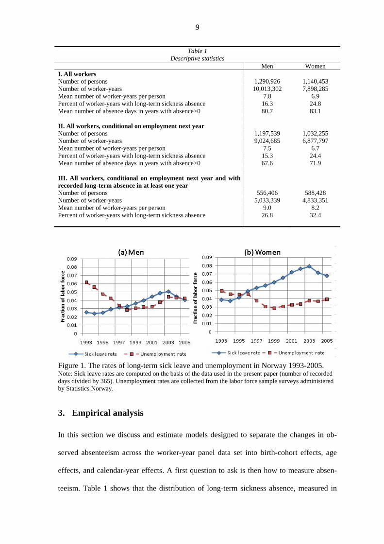
each year. Descriptive statistics for the dataset as a whole are given in Table 1, Panel I. In

total, around 2.4 million workers are included in our data, contributing close to 18 million

worker-years. On average, 16 percent of the men and 25 percent of the women expe-

rience a long-term absence spell each year. And conditional on having such a spell, the

average number of days is 81 for men and 83 for women. Almost half of the workers

have no recorded (long-term) absence spell during our observation window.

To put the development of absenteeism into perspective, Figure 1 shows the time

paths of long-term absence propensities and aggregate unemployment. Long-term absen-

teeism trended upwards until the year 2004. It then declined sharply in response to a

reform of the absence certification regulations which implied stronger activity require-

ments for workers with some remaining work capacity; see Markussen (2009a). Unem-

ployment declined from 1993 to 1998, and remained at a very low level until 2002. Dur-

ing the first half of our observation period, it has previously been suggested that the rec-

orded rise in absenteeism was somehow related to the tight labor market; see, e.g.,

Askildsen et al. (2005) and Nordberg and Røed (2009). However, from 2002 the rates of

absence and unemployment have moved more or less in tandem, which casts some doubt

on the hypothesis of pro-cyclicality in absence rates.

While the statistical analysis of absence behavior is based on the data summarized

in Table 1, we also draw on administrative data describing the evolvement of employ-

ment and disability insurance claims for all Norwegians. These data do not enter directly

into our statistical analysis, but are used to interpret our findings in Section 4 below.

9

Table 1 Descriptive statistics

Men Women I. All workers Number of persons 1,290,926 1,140,453 Number of worker-years 10,013,302 7,898,285 Mean number of worker-years per person 7.8 6.9 Percent of worker-years with long-term sickness absence 16.3 24.8 Mean number of absence days in years with absence>0 80.7 83.1 II. All workers, conditional on employment next year Number of persons 1,197,539 1,032,255 Number of worker-years 9,024,685 6,877,797 Mean number of worker-years per person 7.5 6.7 Percent of worker-years with long-term sickness absence 15.3 24.4 Mean number of absence days in years with absence>0 67.6 71.9 III. All workers, conditional on employment next year and with recorded long-term absence in at least one year

Number of persons 556,406 588,428 Number of worker-years 5,033,339 4,833,351 Mean number of worker-years per person 9.0 8.2 Percent of worker-years with long-term sickness absence 26.8 32.4

Figure 1. The rates of long-term sick leave and unemployment in Norway 1993-2005. Note: Sick leave rates are computed on the basis of the data used in the present paper (number of recorded days divided by 365). Unemployment rates are collected from the labor force sample surveys administered by Statistics Norway.

3. Empirical analysis

In this section we discuss and estimate models designed to separate the changes in ob-

served absenteeism across the worker-year panel data set into birth-cohort effects, age

effects, and calendar-year effects. A first question to ask is then how to measure absen-

teeism. Table 1 shows that the distribution of long-term sickness absence, measured in

10

days, is highly skewed, with an accumulation of zeros, whereas the positive observations

typically represent extensive absence. Therefore, if a fully parametric model were to be

used, the choice of functional form would become a challenge; for instance, a linear re-

gression model intended to explain the number of absence days would inadequately cap-

ture these data features. We also consider the frequency and the duration of spells to be

inappropriate as dependent variables, one reason being that, e.g., a low annual spell fre-

quency can follow from either a very low absence propensity (no absence at all) or a very

high absence propensity (absent all the time). Based on these considerations, we have de-

cided, in our basic empirical model, to explain the probability of experiencing at least

one long-term absence spell during an observation year. To assess robustness, however,

we also report key results when instead using linear regression with the total number of

absence days in each year as the dependent variable.

3.1 Modeling issues

In order to identify separate cohort, age, and time effects, we face two modeling chal-

lenges. The first is the problem of endogenous sorting into and out of our dataset, which

makes the panel grossly unbalanced. As time passes, new cohorts enter employment and

thereby the dataset (sample accretion), while others leave, e.g., due to disability, early

retirement, or death (sample attrition). These events do not occur randomly in relation to

the primary research problem of the study. There is a sorting mechanism which most

likely is correlated with our outcome variable, particularly because the persons who leave

the sample can be expected to be more inclined to be absent – even when belonging to

the same age group – than those staying. To ensure that the sorting problem do not cor-

rupt our attempts to identify time and age effects, we apply a statistical model that con-

trols for unobserved heterogeneity by including individual fixed effects. We recognize

that individual unobserved heterogeneity in absenteeism is generated by a complex (un-

11

modeled) stochastic mechanism, but we condition inference on the values of the hetero-

geneity variables actually realized. As a consequence, we exploit only the within-worker

variation in absenteeism. Specifically, we use a binomial conditional (fixed effects) logit

specification.3 Compared to alternative probability models, the logit model entails the

significant practical advantage that slope coefficients can be consistently estimated with-

out having to estimate the fixed effects (which, in our case would add up to almost 1.5

million coefficients).

The fixed effects approach is not without problems, however. Unbiased inference

requires that, conditional on the fixed effects, the determination of sample inclusion (em-

ployment) logically precedes the determination of sickness absence, i.e. that the joint

model of employment and absenteeism is recursive; see Biørn (2010) for an elaboration.

Although the individual fixed effects can be interpreted as representing all worker-

specific latent factors underlying absenteeism, such as basic health status, work-norm,

occupation, work-environment, and conduct of certifying doctor, to the extent that they

are approximately constant through our observation period, shocks to these variables may

affect both absence propensity and (subsequent) employment. In particular, we worry that

sickness absence may tend to be particularly prevalent in the last year of work-careers,

not only because the risk of being absent in that year is particularly high per se (due to

time and age effects), but also because long-term sickness absence – or the health shock

that triggered it – may cause the work career to end. We deal with this potential problem

by estimating the model without including last-year employment observations; i.e., by

conditioning our worker-year observations on workers being employed in the subsequent

year also. As a result, we lose approximately 10 percent of the male and 13 percent of the

3 This model is described and discussed in, e.g., Chamberlain (1984, Section 3.2), Lechner et al. (2008, Section 7.3), Baltagi (2008, Section 11.1), and Hilbe (2009, Section 13.4.1)

12

female worker-year observations; see descriptive statistics in Table 1, Panel II. While this

strategy may not solve the sorting problem entirely, it provides a sound foundation for

examining its empirical relevance, e.g., by comparing results from the conditional and

unconditional models (where the latter includes last-year employment observations).

The second modeling problem is that our explanatory variables are perfectly col-

linear. By definition, current time minus birth year equals current age. Hence, if these va-

riables occur additively in a (linear or non-linear) model, it apparently becomes impossi-

ble to identify the isolated impact of each variable separately. Technically speaking, this

is due to the fact that for any individual we get only one realization of the data-generating

process in the time domain. It is clearly a challenge to cope with this fundamental identi-

fication problem while seeking to recover potentially interesting “partial” age and time

effects with practical applicability. Even though time-travel is impossible in the real

world, it does make sense as a thought experiment, since the impacts of a purely hypo-

thetical time-travel may convey valuable information regarding the underlying forces be-

hind the rise in absenteeism. Our strategy for solving the multicollinearity problem is

based on the imposition of an additional (minimal) restriction on the age coefficients. But

before we explain that approach in more detail, we set up and estimate the more general

model, where age/time effects are allowed to vary from cohort to cohort. We call this a

“saturated model”, since it fully exploits the degrees of freedom in the time-age space.

The drawback of this general model is that time and age effects become completely inse-

parable, i.e., we can only estimate a single set of time-coefficients for each cohort, which

consequently must be interpreted either as age effects, as time effects or as a combination

of the two. The saturated model nevertheless provides a useful benchmark against which

we can evaluate (and test) the more restrictive model where age and time effects are re-

stricted to be separable and common to all cohorts.

13

3.2 Model selection and specification

Let yit be a dichotomous outcome measure equal to 1 if worker i had at least one long-

term absence spell in year t, and zero otherwise. The imposed logit form of the probabili-

ty implies that the log-odds of absence versus non-absence can be written as:

Pr 1| ,ln ,

Pr 0 | ,

1,..., ; 1928,...,1984; 1993,..., 2005

it ii ct

it i

y t

y t

i N c t

(1)

where i is a worker-specific fixed effect, and ct is the impact of being in year t for

members of cohort c. Note that this setup implies that each year is associated with a sepa-

rate coefficient for each cohort ( )ct . Apart from the imposed logit form with individual

and age/time effects entering additively, there is no functional form restriction on the way

age/time is assumed to affect absence propensity. There is, on the other hand, an impor-

tant restriction embedded in the assumption that the time profiles entering the logit expo-

nentials are the same for all workers belonging to the same cohort. Worker-specific

age/time coefficients ( ct replaced by it ) would have been infeasible, as they cannot be

uncovered from data with only one time series existing for each individual. Note, howev-

er, that the logit structure implies that individual effects and cohort effects actually inte-

ract in the sick-leave probability, though they are separable in the corresponding log-odds

ratio; see, e.g., Greene (2008, Section 23.11.1).

We estimate the cohort-specific age/time effects ( )ct by means of fixed effects

logit model with no less than 541 age/time dummy variables. Due to the inclusion of in-

dividual fixed effects, it is only workers with variation in the outcome variable that can

be used to identify the parameters of interest. Since around 54 percent of the men and 43

percent of the women in our data set never experience long-term absence during our ob-

servation window, the “effective dataset” is reduced to around 1.1 million individuals

14

with 10 million worker-years; see Table 1, Panel III for details. Figure 2 illustrates the

estimation results by taking a closer look at the absence behavior of four of the 57 co-

horts, namely those born in 1940, 1950, 1960, and 1970. These cohorts have in common

that they are observed for all the 13 years in our data-window, but of course at different

ages. In Figure 2, we plot the estimated cohort-specific age/time absence profiles together

with the observed absence rate by year for these four cohorts. Observed absence rates are

plotted for the effective dataset (workers with variation in the outcome variable) as well

as for all workers (including those with no absence in the observation window). The point

estimates are normalized such that all profiles equal observed absence frequencies in the

effective dataset in 1993. The graphs illustrate two important points. First, the rate of

long-term absence has increased significantly over time for members of all the four co-

horts (apart from a decline the last two calendar years), and the calendar-time patterns in

the estimated age/time effects are conspicuously similar across cohorts. For the prime

aged (represented in the graphs by the 1950, 1960, and the 1970 cohorts), in particular,

the age/time effects exhibit a similar time-pattern. This suggests that when pooling dif-

ferent cohorts in the data set, a sensible working hypothesis, potentially useful as an iden-

tification restriction, may be that time and age effects are cohort-invariant. The second

point to note by comparing the three graphs for each cohort in Figure 2 is that there are

large differences between the changes in observed absence behavior within cohorts (as

represented by the data), on the one hand, and the corresponding changes when the indi-

vidual heterogeneiety has been controlled for, i.e., within individuals (as represented by

the estimates), on the other. This suggests that sorting into and out of employment is of

paramount importance for understanding a cohort’s recorded aggregate absence over

time. Unsurprisingly, the sorting process is much more prevalent for older than for

15

younger cohorts: workers with high individual absence propensity are sorted out of em-

ployment as they age, and this sorting process intensifies at higher ages.

Figure 2. Estimated cohort-specific age/time effects from fixed effects model and ob-served absence rates by age and cohort. Selected cohorts only. Note: Estimated age/time effects are normalized by scaling the intercept in Equation (1) such that they are equal to actual absence rates in the (effective) analysis population 1993 (the first observation year for all the cohorts in the graph)

We now turn to a logit model with time and age coefficients a priori restricted to

be cohort invariant, by exploiting the working hypothesis referred to above. By restrict-

ing the model’s time/age pattern in this way, we can circumvent the identification prob-

lem inherent in Equation (1) that time effects perfectly mirror age effects and vice versa.

We retain, however, the worker-specific. The logit model then implies a log-odds ab-

sence versus non-absence ratio of the form

Pr 1| , ,ln ,

Pr 0 | , ,it i it

i t a itit i it

y t aa

y t a

(2)

16

where ita is a vector of age dummies (one for each yearly age). Since time and age is per-

fectly correlated at the individual level, we have a within-group collinearity in Equation

(2).4 Hence, even after imposing a zero restriction on a reference age and on a reference

calendar year, the parameters ( , )t a cannot be readily identified. From Theorem 3.2 in

Kupper et al. (1983) it follows that what can actually be identified in Equation (2) with-

out further restrictions are the differences between pairs of coefficients with the same dis-

tance; see Gaure (2010) for details. To illustrate, let ,a r denote the age coefficient asso-

ciated with age r. We can then readily identify the differences between any two differ-

ences with distance 1: , 1 , , 1 ,( ) ( )a s a s a r a r . However, in order to arrive at inter-

pretable marginal effects, we need to determine the value of a reference difference, in ad-

dition to selecting the trivial reference age. Since this reference acts as a normalization –

not a restriction – it is in some sense immaterial. However, the interpretation of each

coefficient set estimated in this way will depend heavily on which specific ages are se-

lected and the value assigned to the coefficient difference. Let a=r be the immaterial ref-

erence age ,( 0)a r , and let , 1 , , 1( )a r a r a r be the chosen reference difference.

Since every difference of distance 1 is identified, arbitrary differences from our referece

age are also identified by the identity

1

, , , 1 , , 1 , , 1 ,( ) ( ) ( )r S

a r S a r a t a t a r a r a r a rt r

S

(3)

The sum to the right is the partial effect of increasing age by one year from t to t+1, rela-

tive to increasing it from r to r+1. As all the terms on the right hand side are identified by

the above normalization, the left hand side is also identified. It is then clear that if we

4 Let ( , )r rt a be the reference year and reference age, respectively, with r r rc t a . Take a person

in cohort c at time t and age a (so tat t-a=c) with time dummies ( 1 for )j jt t j t and

( 1 for )j ja a j a . We then have that ( ) ( ) ( )r j r j r r rj jj t t j a a t t a a c c , which is

obviously constant within each individual.

17

knew a priori that there were no difference in age effects between r and r+1, we have that

,a r S can be interpreted directly as the effect of changing age from r (or from r+1) to

r+S, holding calendar time constant. If, on the other hand the assumption that

, 1 ,a r a r is incorrect, the interpretation error we make is proportional to the length of

the hypothetical age-travel S. The same considerations hold true for the time coefficients,

but the error is still proportional to the error we make in the interpretation of the age coef-

ficients. That is, the error we make when changing time by the amount S (without chang-

ing age) will be , 1 ,( )a r a rS . Thus, the error in the a priori assumption , 1 ,a r a r

propagates to the time coefficients, and is multiplied by the distance from their reference.

We are indeed going to impose a normalization restriction corresponding to a dif-

ference that we will claim is equal to zero. Note, however, that the model’s statistical va-

lidity – in terms of its ability to fit the data and make predictions – is not at all dependent

on the validity of this assumption. The restriction lies in the interpretation of the distinct

coefficient sets. Hence, its correctness will be crucial for our ability to assess the effects

of hypothetical time- or age traveling, but will have no impact whatsoever on our ability

to assess the overall effects of feasible movements across time and age (since feasible

movements always involve a change in both time and age). The reason why a valid re-

striction on a difference between two coefficients permits us to travel in time is highly

intuitive; if we know a priori that, say, , 1 ,a r a r , then it is obviously the case that the

change in absenteeism occurring as persons of age r become r+1 years identifies the pure

time effect of moving between the corresponding two calendar years. Having identified

the time effects for all years, it is then trivial to identify the remaining age effects.

The normalization we have chosen to apply in the current application builds on

the observation that there is a short age-span for which previous evidence indicates a

constant age effect; see, e.g., Markussen et al. (2009). In particular, there is a short period

18

around the age of 40 where the absence behavior does not seem to change at all and

where employment rates are also virtually constant. In our own data, we indeed find that

within-calendar-year differences in absence rates across all neighboring ages between 35

and 45 are small. Based upon a closer inspection of these differences, we have selected

the assumptions that there are no differences between age 37 and age 38 for men, and no

difference between age 42 and 43 for women.5 To examine the robustness of the resultant

coefficient interpretations, we also present interpretations based on alternative normaliza-

tions. As it turns out, the estimated calendar time and age effects are highly robust to-

wards reasonable variations in the identifying assumptions.

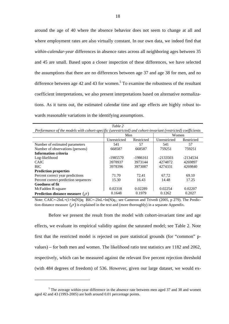
Table 2 Performance of the models with cohort-specific (unrestricted) and cohort-invariant (restricted) coefficients Men Women Unrestricted Restricted Unrestricted Restricted Number of estimated parameters 541 57 541 57 Number of observations (persons) 668587 668587 759251 759251 Information criteria Log-likelihood -1985570 -1986161 -2133503 -2134534 CAIC 3978937 3973144 4274872 4269897 BIC 3978396 3973087 4274331 4269840 Prediction properties Percent correct year predictions 71.70 72.41 67.72 69.10 Percent correct prediction sequences 15.30 16.43 14.48 17.25 Goodness of fit McFadden R-square 0.02318 0.02289 0.02254 0.02207 Prediction distance measure ( ) 0.1648 0.1979 0.1262 0.2027

Note: CAIC=-2lnL+(1+ln(N))q BIC=-2lnL+ln(N)q.; see Cameron and Trivedi (2005, p 279). The Predic-tion distance measure ( ) is explained in the text and (more thoroughly) in a separate Appendix.

Before we present the result from the model with cohort-invariant time and age

effects, we evaluate its empirical validity against the saturated model; see Table 2. Note

first that the restricted model is rejected on pure statistical grounds (for “common” p-

values) – for both men and women. The likelihood ratio test statistics are 1182 and 2062,

respectively, which can be measured against the relevant five percent rejection threshold

(with 484 degrees of freedom) of 536. However, given our large dataset, we would ex-

5 The average within-year difference in the absence rate between men aged 37 and 38 and women aged 42 and 43 (1993-2005) are both around 0.01 percentage points.

19

pect most model restrictions to be rejected, even when they are close approximations to

the true data generating process. The question we want to answer in our case is not really

whether the assumptions of common age and time effects are strictly true, but whether

they represent a sufficiently good approximation to the reality to be of help in our at-

tempts to explain changes in absenteeism over time. The various performance measures

reported in Table 2 indeed indicate that the restricted model performs well. According to

the two information criteria reported (CAIC and BIC), the restricted model clearly out-

performs the saturated model for both men and women.

We also report the two models’ prediction properties. Since the fixed effects

( )i are not identified, we are not able to make an ordinary prediction for each individual.

However, within an individual, the order of the probabilities is identified. If a person has

M observed positive outcomes, the obvious prediction based on our model is that the M

years with the highest probabilities of positive outcomes are observed with this result.

The number reported in Table 2 as “percent correct year predictions” is the percentage of

years with correctly predicted outcome, while the number recorded as “percent correct

prediction sequences” is the percentage of workers with all years correctly predicted. It is

clear from the results reported in Table 2 that the restricted model has higher score ac-

cording to this criterion than the more general model. We also use two measures of

goodness of fit. The first is McFadden's R-square, which is slightly higher for the satu-

rated model, reflecting its larger likelihood. The second ( ) is a prediction distance

measure. For each person we measure the distance between the predicted sequence and

the worst possible prediction. We then compute the normalized Kendall distance, the

number of adjacent exchange operations needed to transform one vector into another, and

normalize by dividing by the distance between the best and worst prediction. Finally, we

rescale such that is zero for random data, 1 for the perfect prediction and -1 for the

20

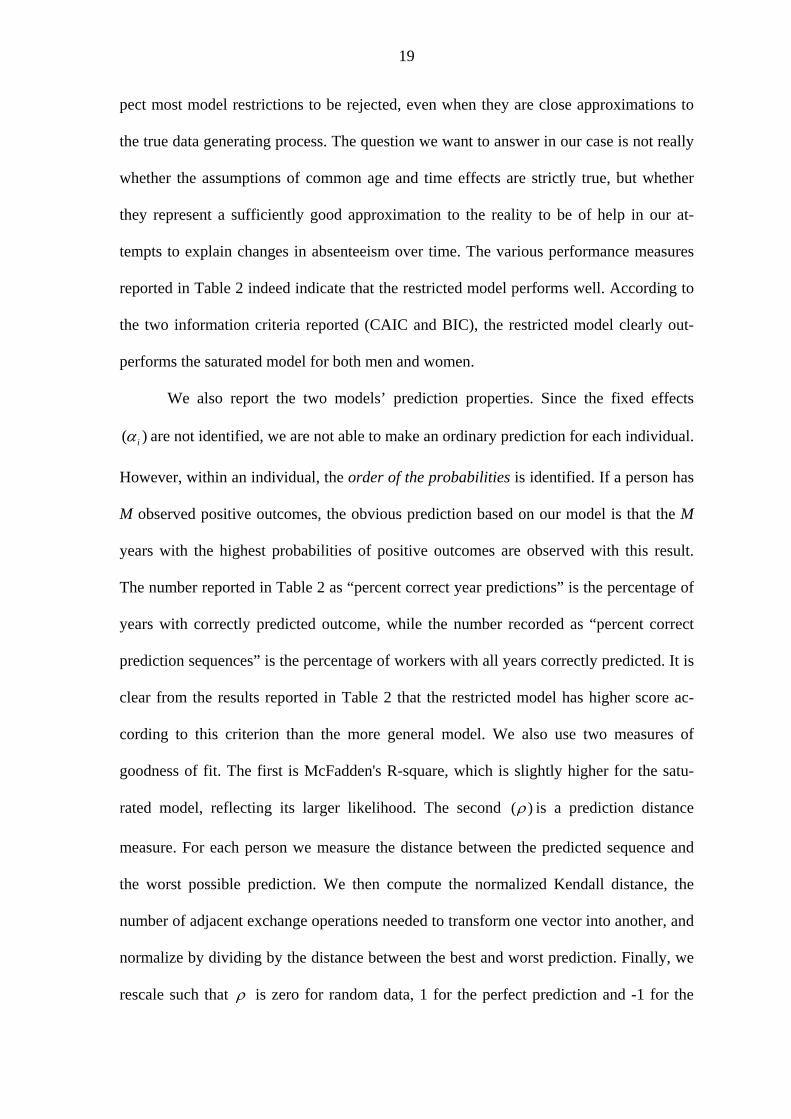
worst possible prediction; see the Appendix for details. Again, we find that the restricted

model outperforms the more general model.

Figure 3. Estimated cohort-specific age/time effects from saturated model and model with cohort-invariant time and age coefficients. Selected cohorts only. Note: Estimated age/time effects are normalized on actual absence rate in 1993 (the first observation year for all the cohorts in the graph)

Another way of assessing the performance of the restricted model is to compare

its cohort-specific age/time profiles with those of the more general model. In Figure 3,

this is done for the same four cohorts that we presented in Figure 2. For men, the re-

stricted model appears to perform extremely well. For women, we note a tendency for the

restricted model to over-estimate the rise in absenteeism for younger cohorts, while it un-

der-estimates it for older cohorts. We nevertheless conclude from these exercises that the

model with cohort-invariant time and age coefficients offers an appropriate tool for a

more detailed examination of the mechanisms behind changes in absenteeism over time.

21

4. Estimation results and implied cohort differences

Estimation results for the restricted model (Equation 2) are presented with 95 percent

confidence intervals. Figure 4 presents the estimated age effects for men and women, re-

spectively, together with the series of observed absence rates by age. Observed absence

rates are again plotted for the analysis population actually used to identify the parameters

of interest as well as for all workers. The point estimates are scaled such that the pre-

dicted absence rate exactly matches the observed absence rate in the (effective) analysis

population at the reference age (37-38 for men, 42-43 for women). It is evident that the

within-individual probability of becoming long-term absent rises much more strongly

with age than the between-individual probability (here represented by the data). The ex-

planation is that early labor market entrants – i.e., those who drop out from school early –

are negatively selected and have higher absence propensities than later entrants. For men,

we see a similar pattern at higher ages. The explanation for this phenomenon is that

workers with high absence propensity are systematically sorted out of the labor market as

they age. It may be noted from Figure 4 that there are some substantial differences in ab-

sence patterns between men and women, both with respect to the overall level and the

age-profile. Except at very young and very old ages, women tend to be much more absent

than men. And unsurprisingly, the difference is particularly marked during the reproduc-

tive phase of women’s lives. While it is natural to interpret the causal age gradient at

higher ages as reflecting deteriorating health, it is perhaps more difficult to understand

the sharp rise in absenteeism at early ages, particularly for men. We speculate that it is

related to tenure, job security, and learning; i.e., that workers make every effort to avoid

unnecessary sickness absence during the initial stages of employment where the cost of

absenteeism is particularly high – in terms of increased layoff risk and poorer career

prospects; see Markussen (2009b).

22

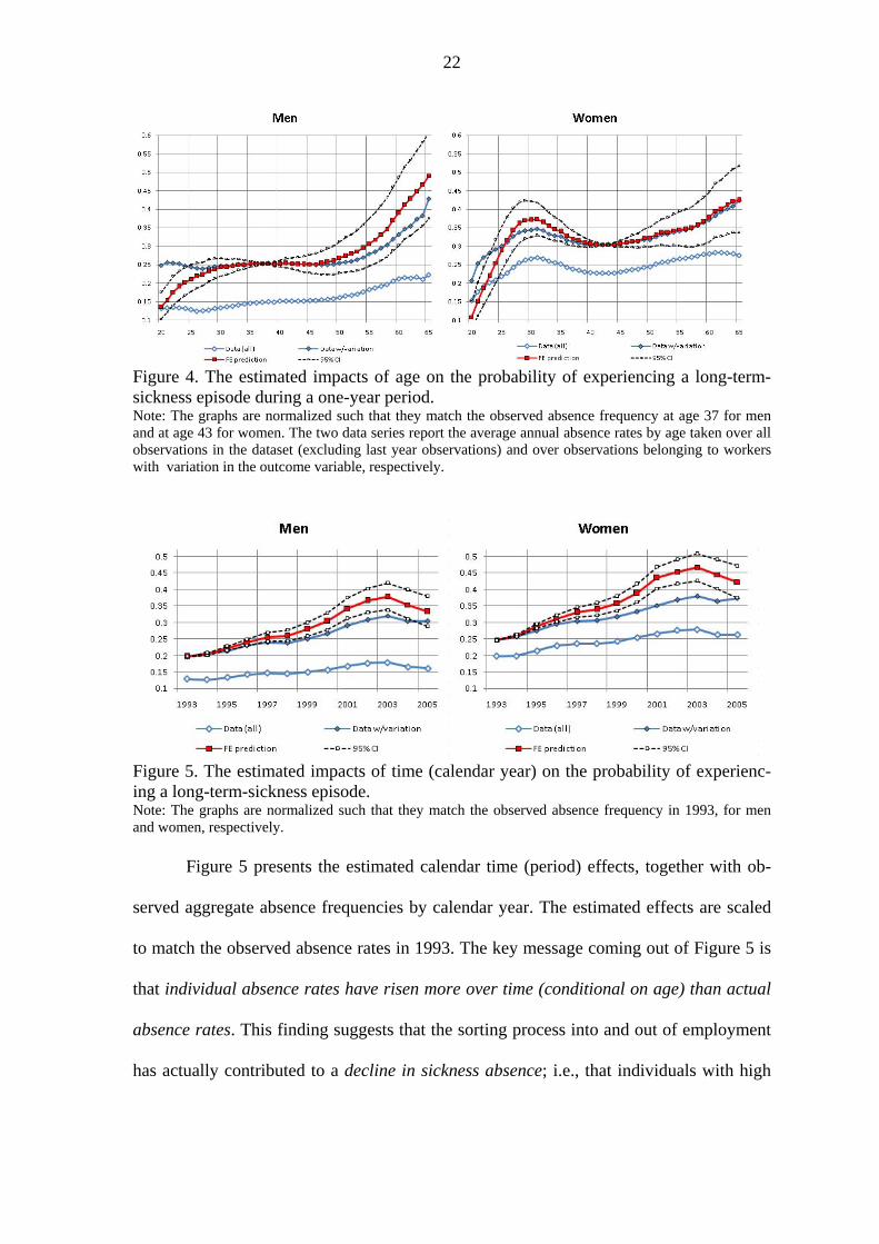
Figure 4. The estimated impacts of age on the probability of experiencing a long-term-sickness episode during a one-year period. Note: The graphs are normalized such that they match the observed absence frequency at age 37 for men and at age 43 for women. The two data series report the average annual absence rates by age taken over all observations in the dataset (excluding last year observations) and over observations belonging to workers with variation in the outcome variable, respectively.

Figure 5. The estimated impacts of time (calendar year) on the probability of experienc-ing a long-term-sickness episode. Note: The graphs are normalized such that they match the observed absence frequency in 1993, for men and women, respectively.

Figure 5 presents the estimated calendar time (period) effects, together with ob-

served aggregate absence frequencies by calendar year. The estimated effects are scaled

to match the observed absence rates in 1993. The key message coming out of Figure 5 is

that individual absence rates have risen more over time (conditional on age) than actual

absence rates. This finding suggests that the sorting process into and out of employment

has actually contributed to a decline in sickness absence; i.e., that individuals with high

23

individual absence propensity have been disproportionably pulled or pushed out of em-

ployment.

Our modeling framework does not offer any simple way of assessing the changes

in absence propensity across cohorts (conditional on time and age), since a cohort’s ab-

sence behavior during a limited time window is bound to reflect both the individual co-

hort-members intrinsic absence propensity and the sorting process determining which of

the cohort members that are employed within the selected time window (the distribution

of individual fixed effects). A cohort’s age-time-adjusted absence behavior may never-

theless convey useful information. Let cty be the observed mean cohort absence rate in a

particular year (including workers with only zero-absence observations); i.e.,

1 ,ctcy itN i c

y y

where ctN is the number of employed workers from cohort c in year t.

We compute a cohort-time-parameter ct by solving the equation

ˆ ˆexp( ) ˆ ˆln

ˆ ˆ 11 exp( )ct t t c ct

ct ct t t cctct t t c

yy

y

. (4)

We then normalize by computing

* exp( )

1 exp( )ct

ctct

, (5)

which summarizes the employed members of cohort c’s absence propensity in year t, ad-

justed for age and time effects. The two upper panels of Figure 6 shows the estimated

age-time adjusted absence propensities in 2005 *2005( )c by birth cohort for men and

women, respectively. The confidence intervals are computed on the basis of the non-

parametric bootstrap; i.e., we have re-sampled (with replacement) and re-estimated the

model 120 times – each time computing new vectors of absence propensities according to

Equations (3) and (4) – and then finally excluded the three most extreme results at each

24

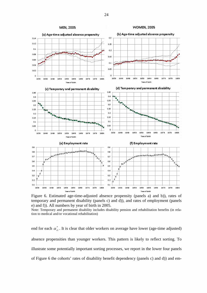
Figure 6. Estimated age-time-adjusted absence propensity (panels a) and b)), rates of temporary and permanent disability (panels c) and d)), and rates of employment (panels e) and f)). All numbers by year of birth in 2005. Note: Temporary and permanent disability includes disability pension and rehabilitation benefits (in rela-tion to medical and/or vocational rehabilitation)

end for each *ct . It is clear that older workers on average have lower (age-time adjusted)

absence propensities than younger workers. This pattern is likely to reflect sorting. To

illustrate some potentially important sorting processes, we report in the lower four panels

of Figure 6 the cohorts’ rates of disability benefit dependency (panels c) and d)) and em-

25

ployment (panels e) and f)) in 2005. The average absence propensity declines as a co-

hort’s employment rate rises during the years of school-to-work transitions (moving from

the extreme right in the graphs). This may suggest that workers who enter the labor mar-

ket in their early 20’s are adversely selected (in terms of their absence propensity). It de-

clines further when the cohort’s employment rate falls during the years of rising disability

benefit dependency (moving towards the extreme left in the graphs). It seems probable

that workers who are still employed in their late 50’s and early 60’s (born before 1955)

are favorably selected.

Given the systematic sorting out of the labor force and thus out of our analysis

population, it is perhaps surprising that the absence propensity among the remaining

workers do not decline more when we move towards the left in Figure 6, from younger to

older cohorts. One possible explanation is simply that younger cohorts are less absent

than older cohorts, ceteris paribus, e.g. because of health improvements or because work-

norms of younger cohorts have improved relative to older cohorts. In order to address the

issue of changes in behavior across cohorts, however, we really need to compare cohorts

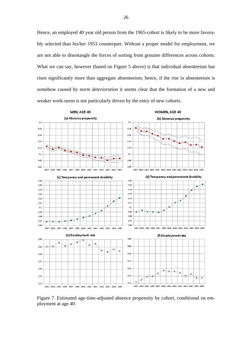
at similar employment levels. Figure 7 provides a comparison of the 1953-1965 birth co-

horts at age 40 (the other cohorts are not observed at age 40 in our data window), at

which point employment rates tend to peak within cohorts. For both men and women, we

find a significant decline in the cohorts’ absence propensity; see panels a) and b). Other

things equal, a member of the 1965-cohort is approximately 30 percent less likely to have

a long-term absence spell during a year than a member of the 1953-cohort. This finding

does apparently not support the idea that younger cohorts subscribe to a weaker work-

norm than older cohorts. However, Figure 7 also shows that there has been a tremendous

rise in disability rates at age 40 over these 13 birth-cohorts (panels b) and c)), and from

the 1960-cohort and onwards, there has also been a slight decline in employment rates.

26

Hence, an employed 40 year old person from the 1965-cohort is likely to be more favora-

bly selected than his/her 1953 counterpart. Without a proper model for employment, we

are not able to disentangle the forces of sorting from genuine differences across cohorts.

What we can say, however (based on Figure 5 above) is that individual absenteeism has

risen significantly more than aggregate absenteeism; hence, if the rise in absenteeism is

somehow caused by norm deterioration it seems clear that the formation of a new and

weaker work-norm is not particularly driven by the entry of new cohorts.

Figure 7. Estimated age-time-adjusted absence propensity by cohort, conditional on em-ployment at age 40.

27

5. Robustness

In this section, we examine the robustness of our results with respect to i) the inclusion of

individuals’ last employment year in the estimation, ii) the selection of interpretation re-

striction facilitating travels in time and age, and iii) the selection of outcome measure and

functional form. We focus on the robustness of the calendar year coefficients in this sec-

tion, given that these are the coefficients of greatest interest and noting that the degree of

robustness tends to be similar for the time and age coefficients. Note, however, that since

interpretation errors are proportional to the length of the time- or age travel, our age pro-

files are less robust towards interpretation errors than the time profiles for the simple rea-

son that they involve much longer journeys (while the estimated time-profile covers 13

years, the age profile covers 47 years).

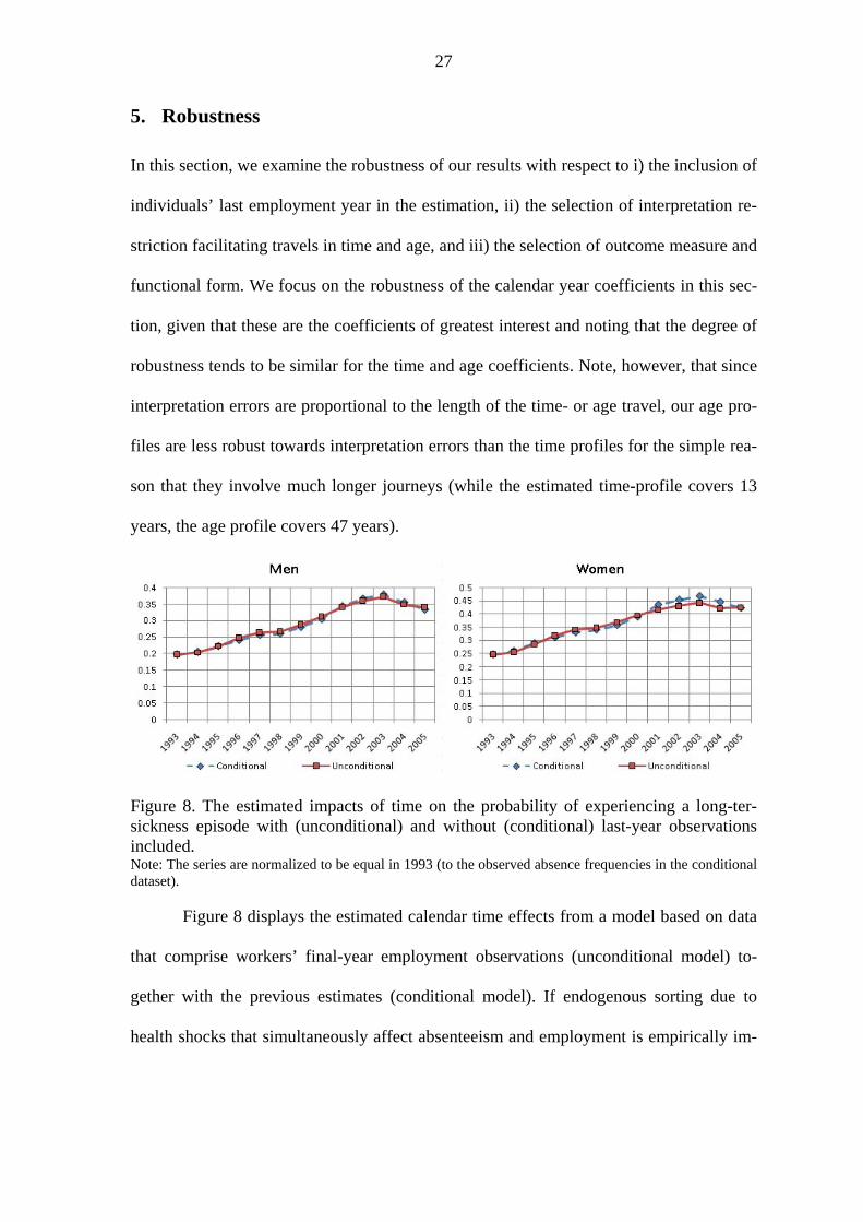
Figure 8. The estimated impacts of time on the probability of experiencing a long-ter- sickness episode with (unconditional) and without (conditional) last-year observations included. Note: The series are normalized to be equal in 1993 (to the observed absence frequencies in the conditional dataset). Figure 8 displays the estimated calendar time effects from a model based on data

that comprise workers’ final-year employment observations (unconditional model) to-

gether with the previous estimates (conditional model). If endogenous sorting due to

health shocks that simultaneously affect absenteeism and employment is empirically im-

28

portant, we would expect the inclusion of final-year observations to change results signif-

icantly. As it turns out, it does not. For men, the two series are hardly distinguishable.

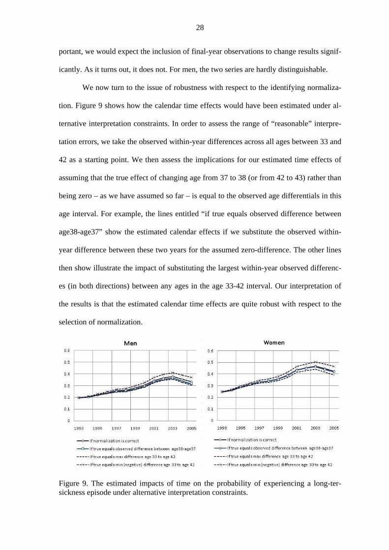
We now turn to the issue of robustness with respect to the identifying normaliza-

tion. Figure 9 shows how the calendar time effects would have been estimated under al-

ternative interpretation constraints. In order to assess the range of “reasonable” interpre-

tation errors, we take the observed within-year differences across all ages between 33 and

42 as a starting point. We then assess the implications for our estimated time effects of

assuming that the true effect of changing age from 37 to 38 (or from 42 to 43) rather than

being zero – as we have assumed so far – is equal to the observed age differentials in this

age interval. For example, the lines entitled “if true equals observed difference between

age38-age37” show the estimated calendar effects if we substitute the observed within-

year difference between these two years for the assumed zero-difference. The other lines

then show illustrate the impact of substituting the largest within-year observed differenc-

es (in both directions) between any ages in the age 33-42 interval. Our interpretation of

the results is that the estimated calendar time effects are quite robust with respect to the

selection of normalization.

Figure 9. The estimated impacts of time on the probability of experiencing a long-ter- sickness episode under alternative interpretation constraints.

29

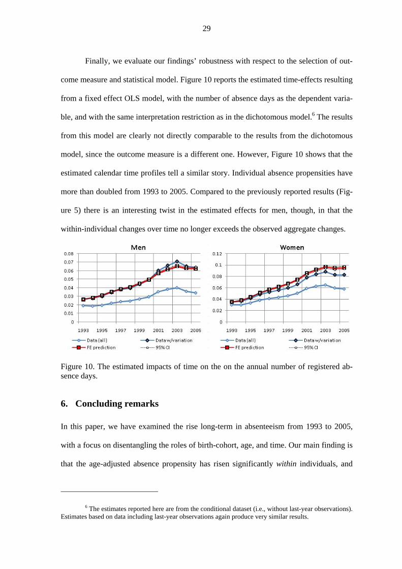
Finally, we evaluate our findings’ robustness with respect to the selection of out-

come measure and statistical model. Figure 10 reports the estimated time-effects resulting

from a fixed effect OLS model, with the number of absence days as the dependent varia-

ble, and with the same interpretation restriction as in the dichotomous model.6 The results

from this model are clearly not directly comparable to the results from the dichotomous

model, since the outcome measure is a different one. However, Figure 10 shows that the

estimated calendar time profiles tell a similar story. Individual absence propensities have

more than doubled from 1993 to 2005. Compared to the previously reported results (Fig-

ure 5) there is an interesting twist in the estimated effects for men, though, in that the

within-individual changes over time no longer exceeds the observed aggregate changes.

Figure 10. The estimated impacts of time on the on the annual number of registered ab-sence days.

6. Concluding remarks

In this paper, we have examined the rise long-term in absenteeism from 1993 to 2005,

with a focus on disentangling the roles of birth-cohort, age, and time. Our main finding is

that the age-adjusted absence propensity has risen significantly within individuals, and

6 The estimates reported here are from the conditional dataset (i.e., without last-year observations). Estimates based on data including last-year observations again produce very similar results.

30

this within-individual rise is actually larger than the aggregate rise in absenteeism. While

this finding does not allow us to identify a particular causal mechanism, it does make it

possible to rule out some popular explanations. We can reject the popular hypothesis that

the rise in absenteeism resulted from the entry of new cohorts into the labor market with

weaker work-norms than older cohorts. We can also reject the potentially reassuring idea

that it resulted from successful integration of marginal workers with poor health into the

workforce. Our findings actually point to the contrary; i.e., that workers with high ab-

sence propensity have been systematically sorted out of the labor market. This finding is

consistent with the fact that the fraction of the working-age population who were inactive

due to permanent or temporary disability rose markedly in during our data period, from

around 12 percent in 1993 to 16 percent in 2005. Our findings may thus indicate that the

problem of rising absenteeism among the still-employed workers in Norway is even more

worrying than indicated by aggregate statistics.

References

Askildsen, J. E., Bratberg, E. and Nilsen, Ø. A. (2005) Unemployment, Labour Force

Composition and Sickness Absence. A Panel Data Study. Health Economics, Vol.

14, No. 11, 1087-1101.

Baltagi, B. H. (2008) Econometric Analysis of Panel Data, Fourth Edition, Chichester: Wiley

Biørn, E. (2010) Identifying Trend and Age Effects in Sickness Absence from Individual

Data. Some Econometric Problems. Memorandum, Department of Economics,

University of Oslo.

Cameron, A. C and Trivedi, P. K. (2005) Microeconometrics. Methods and Applications.

Cambridge University Press, New York.

Chamberlain, G. (1984) Panel Data. In Handbook of Econometrics, Vol. 2, ed. by Z Gril-

31

liches and M. D. Intriligator. Amsterdam: North Holland, 1247-1318.

Gans, D., and Silverstein, M. (2006) Norms of Filial Responsibility for Aging Parents

Across Time and Generations. Journal of Marriage and Family, 68, 961-976.

Gaure, S. (2010) Dummy-encoding of Inherently Collinear Variables. Working Paper. In

progress.

Greene, W. H. (2008) Econometric Analysis. Sixth Edition. New Jersey. Prentice Hall.

Hilbe, J. M. (2009) Logistic Regression Models. New York: Chapman & Hall/CRC Press.

Ihlebaek, C., Brage, S., and Eriksen, H. R. (2007) Health Complaints and Sickness Ab-

sence in Norway, 1996-2003. Occupational Medicine, 57, 43-49.

Kupper, L. L., Janis, J. M., Salama, I. A., Yoshizawa, C. N. and Greenberg, B. G. (1983)

Age-Period-Cohort Analysis: An Illustration of the Problems in Assessing Inte-

raction in One Observation per Cell Data. Commun. Statist.-Theor. Meth. Vol. 12,

No. 23, 2779-2807.

Lechner, M., Lollivier, S., and Magnac, T. (2008) Parametric Binary Choice Models.

Chapter 7 in The Econometrics of Panel Data. Fundamentals and Recent

Developments in Theory and Practice, Third Edition, Heidelberg: Springer.

Lindbeck, A. (1995) Hazardous Welfare-State Dynamics. American Economic Review,

Papers and Proceedings, 85, 9-15.

Lindbeck, A., Nyberg, S., and Weibull, J. W. (1999) Social Norms and Economic Incen-

tives in the Welfare State. Quarterly Journal of Economics, 114, 1-35.

Markussen, S. (2009a) Closing the Gates? Evidence from a Natural Experiment on Phy-

sicians' Sickness Certification. Memorandum No. 19/2009, Department of Eco-

nomics, University of Oslo.

Markussen, S. (2009b) The Effects of Sick-Leaves on Earnings. Memorandum No.

20/2009, Department of Economics, University of Oslo.

32

Markussen, S., Røed, K., Røgeberg, O. J., and Gaure, S. (2009) The Anatomy of Absen-

teeism. IZA Discussion Paper No. 4240.

Nordberg, M. and Røed, K. (2009) Economic Incentives, Business Cycles, and Long-

Term Sickness Absence. Industrial Relations, Vol. 48, No. 2, 203-230.

Ryder, N. B. (1965) The Cohort as a Concept in the Study of Social Change. American

Sociological Review, 30, 843-861.

Appendix: The prediction distance measure ( )

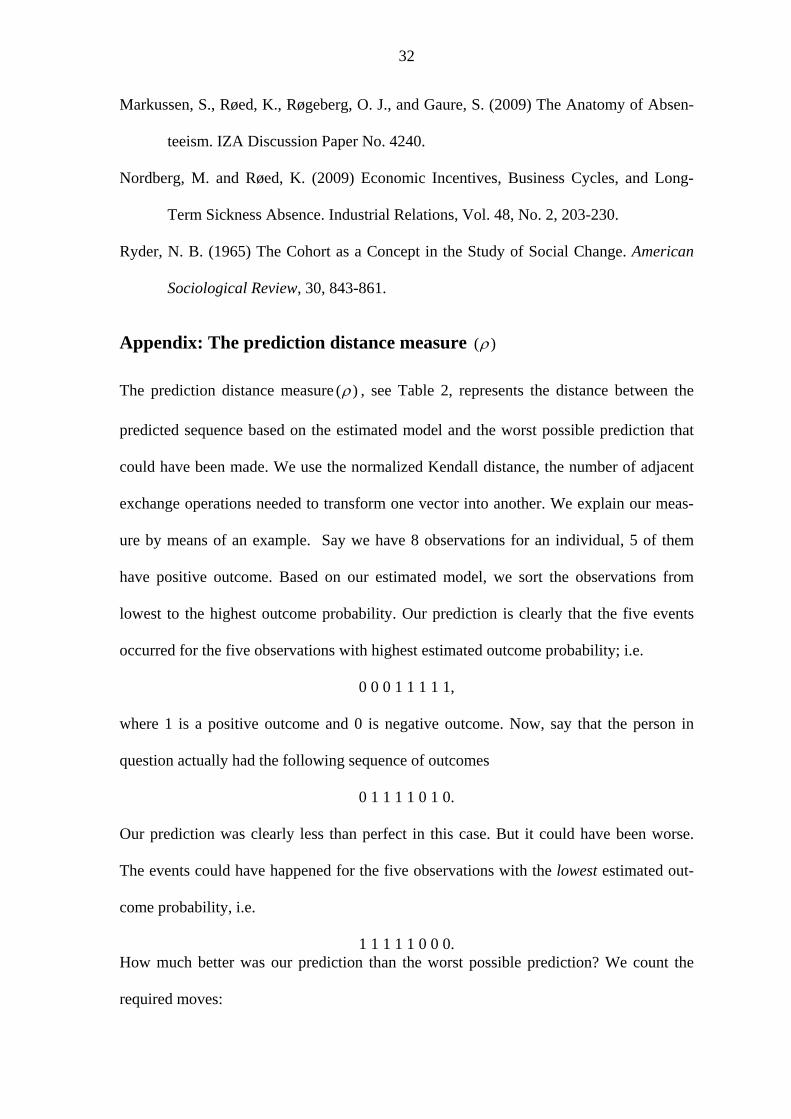
The prediction distance measure ( ) , see Table 2, represents the distance between the

predicted sequence based on the estimated model and the worst possible prediction that

could have been made. We use the normalized Kendall distance, the number of adjacent

exchange operations needed to transform one vector into another. We explain our meas-

ure by means of an example. Say we have 8 observations for an individual, 5 of them

have positive outcome. Based on our estimated model, we sort the observations from

lowest to the highest outcome probability. Our prediction is clearly that the five events

occurred for the five observations with highest estimated outcome probability; i.e.

0 0 0 1 1 1 1 1,

where 1 is a positive outcome and 0 is negative outcome. Now, say that the person in

question actually had the following sequence of outcomes

0 1 1 1 1 0 1 0.

Our prediction was clearly less than perfect in this case. But it could have been worse.

The events could have happened for the five observations with the lowest estimated out-

come probability, i.e.

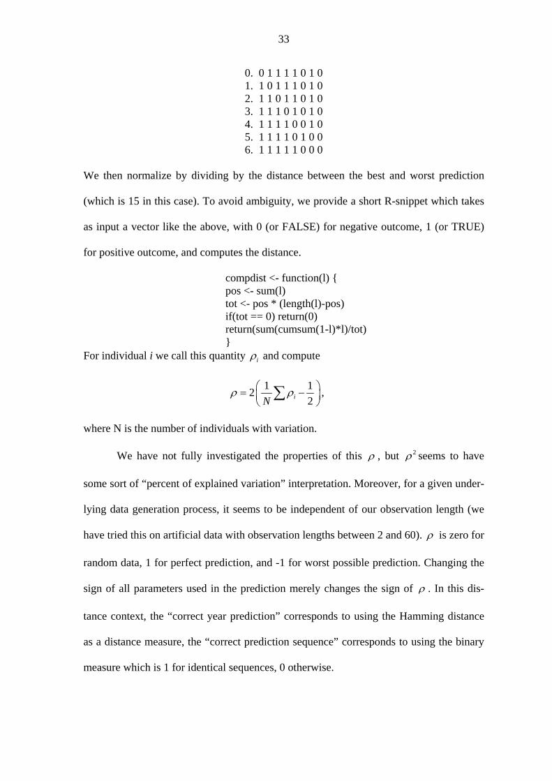
1 1 1 1 1 0 0 0. How much better was our prediction than the worst possible prediction? We count the

required moves:

33

0. 0 1 1 1 1 0 1 0 1. 1 0 1 1 1 0 1 0 2. 1 1 0 1 1 0 1 0 3. 1 1 1 0 1 0 1 0 4. 1 1 1 1 0 0 1 0 5. 1 1 1 1 0 1 0 0 6. 1 1 1 1 1 0 0 0

We then normalize by dividing by the distance between the best and worst prediction

(which is 15 in this case). To avoid ambiguity, we provide a short R-snippet which takes

as input a vector like the above, with 0 (or FALSE) for negative outcome, 1 (or TRUE)

for positive outcome, and computes the distance.

compdist <- function(l) { pos <- sum(l) tot <- pos * (length(l)-pos) if(tot == 0) return(0) return(sum(cumsum(1-l)*l)/tot) }

For individual i we call this quantity i and compute

1 1

22iN

,

where N is the number of individuals with variation.

We have not fully investigated the properties of this , but 2 seems to have

some sort of “percent of explained variation” interpretation. Moreover, for a given under-

lying data generation process, it seems to be independent of our observation length (we

have tried this on artificial data with observation lengths between 2 and 60). is zero for

random data, 1 for perfect prediction, and -1 for worst possible prediction. Changing the

sign of all parameters used in the prediction merely changes the sign of . In this dis-

tance context, the “correct year prediction” corresponds to using the Hamming distance

as a distance measure, the “correct prediction sequence” corresponds to using the binary

measure which is 1 for identical sequences, 0 otherwise.