6971 2018

March 2018

The Rise and Fall of Bioenergy Michael Hoel

Impressum:  

CESifo Working Papers ISSN 2364‐1428 (electronic version) Publisher and distributor: Munich Society for the Promotion of Economic Research ‐ CESifo GmbH The international platform of Ludwigs‐Maximilians University’s Center for Economic Studies and the ifo Institute Poschingerstr. 5, 81679 Munich, Germany Telephone +49 (0)89 2180‐2740, Telefax +49 (0)89 2180‐17845, email office@cesifo.de Editors: Clemens Fuest, Oliver Falck, Jasmin Gröschl www.cesifo‐group.org/wp   An electronic version of the paper may be downloaded  ∙ from the SSRN website:           www.SSRN.com ∙ from the RePEc website:          www.RePEc.org ∙ from the CESifo website:         www.CESifo‐group.org/wp    

 

CESifo Working Paper No. 6971 Category 10: Energy and Climate Economics

The Rise and Fall of Bioenergy

Abstract If bioenergy has a less negative impact on the climate than fossil energy, it may be optimal to have a significant increase in the use of bioenergy over time. Due to the difference in the way the climate is affected by the two types of energy, the future time path of the use of bioenergy may be non-monotonic: It may be optimal to first have an increase in its use, and later a reduction. Optimal taxes and subsidies are derived both for the first-best case and for the case of a constraint on the size of the fossil tax.

JEL-Codes: Q420, Q480, Q540, Q580.

Keywords: bioenergy, renewable energy, climate policy, carbon tax, second best, subsidies.

Michael Hoel

Department of Economics University of Oslo

P.O. Box 1095, Blindern Norway – 0317 Oslo mihoel@econ.uio.no

March 20, 2018 I gratefully acknowledge comments and suggestions from participants at conferences and seminars in Athens, Geilo, Munich, Oslo, Tilburg and Umeå. While carrying out this research I have been associated with CREE -Oslo Centre for Research on Environmentally friendly Energy. CREE is supported by the Research Council of Norway.

1 Introduction

In many countries there are various forms of direct and indirect subsidies

to biofuels and other types of bioenergy. Such policies are often justified by

an argument that bioenergy is "climate neutral", and that the production

and use of bioenergy gives a reduction in the use of fossil energy. There

are two problems with these arguments. First, recent contributions have

questioned whether the production and use of bioenergy is climate neutral

in the sense that it has no climate impact. Moreover, even if the production

and use of bioenergy had no climate impact, the argument for subsidizing

it is questionable. It is widely recognized among economists that a price

on carbon emissions, through a carbon tax or a price on tradeable emission

permits, is the most important policy instrument to reduce such emissions.

Standard economic reasoning also implies that in the absence of other market

failures, an appropriately set carbon price is the only instrument needed to

achieve an effi cient climate policy. If bioenergy had no direct climate impact,

it should therefore be neither taxed nor subsidized. A possible reason for

subsidizing bioenergy could be that tax on fossil energy is "too low", i.e.

lower than the Pigovian rate (equal to the marginal environmental cost of

carbon emissions).

To study these issues, this paper considers a simple model where fossil

fuels (henceforth called fossil energy) and bioenergy are perfect substitutes.

The climate effects of the two types of energy are discussed in Section 2.

Unlike fossil energy, bioenergy is climate neutral in the sense that it is possible

to have a constant positive use of bioenergy without this giving any change

over time in the carbon concentration in the atmosphere. This implies that

in a long-run steady state, we will (under conditions specified in section 3)

have positive bioenergy production and zero fossil energy production.

Although bioenergy is climate neutral in the sense given above, it has a

negative climate impact in the sense that for any given time path of fossil

energy, the carbon in the atmosphere is higher the higher is the level of the

2

time path (constant or varying over time) of the production of bioenergy.

Hence, both fossil energy and bioenergy have a negative climate impact, but

the dynamics of these impacts differ. In section 3 the first-best optimum is

derived, and it is shown that fossil energy production is zero in the long run,

while bioenergy production is positive and constant. Due to the difference

in how the climate is affected by the two types of energy, the time path of

bioenergy production towards its steady-state level may be non-monotonic.

Particular attention is given to the case in which marginal climate costs have

an inverse L property: zero (or small) for carbon contents in the atmosphere

below some threshold, and rapidly rising after the threshold is reached. In

this case bioenergy production will first rise, and later decline towards its

steady-state level.

To achieve the first-best optimum, bioenergy must have a non-negative

tax. In the limiting case of zero marginal climate costs for low levels of

carbon in the atmosphere the tax will be zero initially, but will eventually

become positive.

As mentioned above, the tax on fossil energy could for some reason be

constrained to be lower than its optimal value. The implications of such

a constraint for bioenergy production and bioenergy policies are studies in

section 4. In particular, it is shown that in this case it may be optimal to

subsidize bioenergy for all or some of the time. For the inverse L climate

cost function, it is optimal to subsidize bioenergy as long as carbon in the

atmosphere is below the threshold. Moreover, during this phase the subsidy

is increasing over time. However, once the threshold is reached the subsidy

will start to decline. In the long run the tax on bioenergy may be negative

(i.e. a subsidy) or positive, depending on parameters of the model.

Section 5 discusses the climate dynamics of bioenergy production in more

detail, before Section 6 concludes.

3

1.1 Related literature

While the present study focuses on taxes and subsidies as policy instruments,

there are several studies on the effects of a renewable portfolio standard

for bioenergy. A renewable portfolio standard in this case means that a

certain politically determined minimum percentage of the total energy use

must come from bioenergy. Such a renewable portfolio standard is equivalent

to a revenue neutral combination of a tax on fossil energy and a subsidy to

bioenergy, see e.g. Amundsen and Mortensen (2001) and Eggert and Greaker

(2012). A combination of a tax on fossil energy and a subsidy may be (second-

best) optimal if there is a constraint on the tax on fossil energy (see Section

4), but this combination will generally not be revenue neutral.

De Gorter and Just (2009) find that a renewable fuel standard may lead

to a decrease in the total use of fuel (oil and biofuel). This happens if the

elasticity of biofuels supply is lower than the elasticity of oil supply. The

effect of the policy is in this case not only to replace oil with biofuels, but

also to reduce total consumption of transport fuels, which by itself will reduce

climate costs. This result is reversed if the elasticity of biofuels supply is

higher than the elasticity of oil supply, or if a biofuels subsidy is imposed

rather than a renewable fuel standard.

If a renewable fuel standard is in place, adding a subsidy or a tax rebate

for biofuels will increase climate costs, even if there were no negative climate

effects from bioenergy. The reason is that if the ratio between fossil energy

and bioenergy is fixed due to the renewable portfolio standard, a subsidy to

bioenergy works as an implicit support to oil and, hence, GHG emissions

increase (see DeGorter and Just, 2010). The effects of combining several

policies related to bioenergy have also been studied by Eggert and Greaker

(2012) and Lapan and Moschini (2012).

Lapan and Moschini (2012) compare a renewable fuel standard with a

subsidy to biofuels, and find that the former welfare dominates the latter.

This result follows directly from the fact that a renewable fuel standard is

4

identical to a revenue neutral combination of a tax on oil and a subsidy to

biofuels, since there is an emission externality from the use of fossil fuels.

There are some contributions in the literature that analyze bioenergy poli-

cies in models with dynamic oil supply, see e.g. Chakravorty et al. (2008),

Chakravorty and Hubert (2013), Grafton et al. (2012), and Fischer and

Salant (2012). However, none of these studies includes negative climate ef-

fects from the use of bioenergy, which seems to be crucial when assessing the

effect of bioenergy policies on climate costs.

Climate effects from bioenergy are included in the analysis of Greaker et

al. (2014), where cumulative oil extraction depends on the policies used. An

important result is that whereas a non-declining tax on oil or a non-declining

subsidy to biofuel reduces cumulative oil extraction, a blending share has no

effect on cumulative oil extraction (as long as the implied share of fossil

is bounded away from zero). Such a blending mandate may nevertheless

contribute to lower GHG emissions, as this policy will increase consumer

prices and hence reduce the total fuel use at any time.

While most studies of bioenergy consider bioenergy from fuel crops, an

alternative is to use the harvest from standing forest to produce bioenergy.

Hoel and Sletten (2016) study climate policies for this type of bioenergy

when it is assumed to be a perfect substitute for fossil energy (as assumed

in the present study). However, unlike the present study they assume that

the relative climate impact of the two types of energy are constant over time.

Moreover, their main focus is on the long-run steady state, where there is no

production of fossil energy.

5

2 The climate effects of carbon energy and

bioenergy

The climate is affected by the amount of carbon in the atmosphere, and

burning of fossil fuels (i.e. the use of fossil energy) adds carbon to the at-

mosphere. As we shall see below, this is true also for bioenergy, although the

mechanism is somewhat different. For both types of energy, the model I use

gives a very crude and simple description of how the atmospheric carbon is

affected. The following quotation from Millner (2015) might help to justify

the somewhat drastic simplifications I use: "Like many economic models, our

is a fable in which reality is pushed to absurdly simplistic extremes in order

to cleanly illustrate a mechanism that may help explain real world policy

outcomes."

2.1 Atmospheric carbon from fossil energy

Using carbon energy gives an immediate release of carbon to the atmosphere.

Over time, some of this carbon is transferred to the ocean and other sinks.

However, a significant portion (about 25% according to e.g. Archer, 2005)

remains in the atmosphere for ever (or at least for thousands of years). In this

paper I simply assume that all the carbon released remains in the atmosphere

for ever. This simplification is of no importance for the long-run steady state,

but the details of the dynamics towards the steady state would be slightly

different if I had taken the partial depreciation into account.

In my model, x(t) measures the yearly production of fossil energy, and

Sx(t) measures the stock of carbon in the atmosphere caused by the produc-

tion of fossil energy. The relationship between the two is simply Sx(t) = x(t).

The dynamics of carbon in the atmosphere from fossil energy production is

illustrated in Figure 1. In this figure we first have constant production, then

production jumps up to a higher level, and finally it drops to low level. The

important point (to be contrasted with bioenergy production below) is that

6

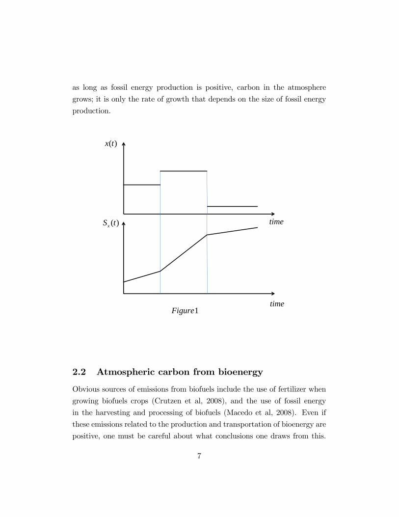
as long as fossil energy production is positive, carbon in the atmosphere

grows; it is only the rate of growth that depends on the size of fossil energy

production.

time

( )x t

( )xS t

1Figuretime

2.2 Atmospheric carbon from bioenergy

Obvious sources of emissions from biofuels include the use of fertilizer when

growing biofuels crops (Crutzen et al, 2008), and the use of fossil energy

in the harvesting and processing of biofuels (Macedo et al, 2008). Even if

these emissions related to the production and transportation of bioenergy are

positive, one must be careful about what conclusions one draws from this.

7

There are, after all, emissions related to practically all economic activity. It

is only if the emissions related to production and transportation of bioenergy

are larger per unit of general resources used (labor, capital etc.) than the

emissions related to these resources being used elsewhere in the economy that

one can conclude that increased use of bioenergy contributes to increased

climate costs.

Perhaps the most important source of greenhouse gas emissions from

bioenergy is related to land use changes. As pointed out by e. g. Fargione et

al. (2008), converting forests, peatlands, savannas, or grasslands to produce

crop-based bioenergy will give a large immediate release of carbon from plant

biomass and soils to the atmosphere.

In many cases bioenergy crops are grown on existing agricultural land, so

that there is little or no direct effect on carbon emissions. However, increasing

the production of bioenergy crops at the expense of food production raises

other concerns: Food prices may increase, with negative consequences for

low-income households world wide (see e.g. Chakravorty et al., 2008, and

Chakravorty et al., 2009). Moreover, reduced land for food production may

cause indirect land use changes: The increased value of land used for food

production may lead to forest clearing to convert land for food production.

This forest clearing will have the immediate effect of releasing carbon to the

atmosphere, and thus increase climate costs. Both Searchinger et al. (2008)

and Lapola et al. (2010) analyze indirect land-use change, and show that the

effect upon emissions may be of great significance.

In my model I treat direct land-use change and indirect land-use change

together. In particular, I assume that each unit of bioenergy production

requires ` units of land, and that each unit of land converted to bioenergy

production will reduce the carbon sequestered on this land by an amount

σ. Increasing the yearly production of bioenergy by one unit hence gives a

one-off increase in the amount of carbon in the atmosphere by σ` ≡ β units.

In the model, fossil energy and bioenergy are measured in the same units,

8

with 1 unit being equal to the amount of fossil energy that releases 1 unit of

carbon to the atmosphere. Hence the denomination of y is tons of carbon per

year. The denomination of ` is land units per y, and the denomination of σ is

tons of carbon per land unit. Hence, the denomination of β is tons of carbon

per y, i.e. tons of carbon/(tons of carbon per year), i.e. "years". Using this

approach, Greaker et al. (2014) show that estimates in the literature of `

and σ suggest that β typically will be in the range of about 9-24 years.

In the reasoning above it has been implicitly assumed that bioenergy is

based on fuel crops. An alternative to converting grazing land or forest land

into land for growing suitable crops for bioenergy production is to use the

harvests from standing forests to produce bioenergy. However, wood-based

bioenergy from standing forests is not unproblematic from a climatic point

of view. The carbon stored in the forest is highest when there is little or no

harvest from the forest, see e.g. van Kooten et al. (1995), or more recently,

Hoel et al. (2014) and the literature cited there. Hence, increasing the

harvest from a forest in order to produce more bioenergy may conflict with

the direct benefit of the forest as a sink of carbon.

Wood-based bioenergy may take many forms, including e.g. raw firewood,

processed charcoals, and pellets. The possibility of producing liquid bioen-

ergy from cellulosic biomass may also be a promising alternative to using fuel

crops, see e.g. Hill et al. (2006). To the extent that bioenergy is produced

from residuals that otherwise would gradually rot and release carbon, the

climate impact of this type of bioenergy is limited. If increased production

of bioenergy implies increased harvesting from the forest, the time path of

the carbon in the forest biomass will be shifted downwards, giving an un-

ambiguously negative climate effect (i.e. increased climate costs). This is

illustrated in figure 2, where g(F ) is a standard biological growth function

showing the growth of the forest as a function of its volume F (measured in

tons of carbon). With harvesting h the net growth is hence g(F )− h.

9

F

g( ),F h

F**F *F

**h*h

( )g F

2Figure

If yearly harvesting increases from a constant value h∗ to a new constant

value h∗∗, the forest volume will eventually decline from F ∗ = g−1(h∗) to

F ∗∗ = g−1(h∗∗). Assume that one unit increased bioenergy production im-

plies φ units increased harvest, implying that one unit permanent increase

of bioenergy production will give a permanent reduction of the volume of

the forest equal to −φ(g′)−1(h). Moreover, assume that a fraction ξ of the

carbon released from the forest is permanently added to the carbon in the

atmosphere. Then one unit permanent increase of bioenergy production will

give an immediate and permanent increase in the carbon in the atmosphere

equal to −ξφ(g′)−1(h) ≡ β. Also in this case, β is measured in years, and

in this case it will depend strongly on how intensively the forest initially is

harvested. If the initial harvest h is close to the maximal sustainable yield

10

value (i.e. close to max g(F )), −g′ will be small and hence −(g′)−1 and β

will be large.

In my model, y(t) measures the yearly production of bioenergy, and Sy(t)

measures the stock of carbon in the atmosphere caused by the production

of carbon energy. The relationship between the two is simply Sy(t) = βy(t).

Although such a relationship might be reasonable in the long run, it is of

course quite a drastic simplification in the short run. The relationship is

illustrated by the heavily drawn curve in Figure 3, with a similar time pattern

of energy production as for fossil energy production in Figure 1. The level

of carbon in the atmosphere depends on the size of bioenergy production,

but as long as bioenergy production is constant, carbon in the atmosphere

is also constant. This is in sharp contrast to the case of fossil fuel illustrated

in Figure 1, where carbon in the atmosphere was growing for any positive

production level.

11

time

y( )t

( )yS t

3Figuretime

In the formal model, and in Figure 3, a change in y(t) from one constant

level y1 to a new constant level y2 will immediately change Sy(t) from βy1

to βy2. In reality, the change in the amount of carbon to a new long-run

level will not be immediate. Hence, the adjustment is likely to look more like

the case illustrated by the dashed lines in Figure 3. I return to this issue in

Section 5, and discuss when the differences between the two cases (solid and

dashed curves in Figure 3) may be qualitatively important.

12

3 The optimal use of bioenergy

3.1 The model

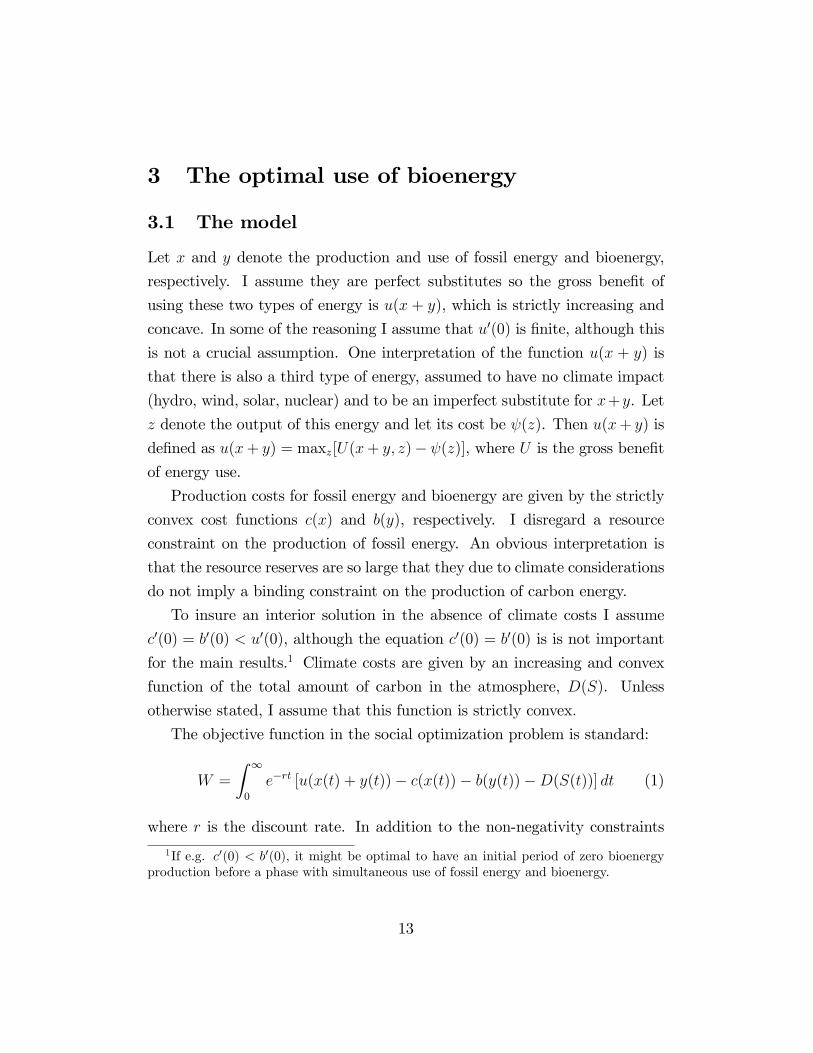
Let x and y denote the production and use of fossil energy and bioenergy,

respectively. I assume they are perfect substitutes so the gross benefit of

using these two types of energy is u(x + y), which is strictly increasing and

concave. In some of the reasoning I assume that u′(0) is finite, although this

is not a crucial assumption. One interpretation of the function u(x + y) is

that there is also a third type of energy, assumed to have no climate impact

(hydro, wind, solar, nuclear) and to be an imperfect substitute for x+y. Let

z denote the output of this energy and let its cost be ψ(z). Then u(x+ y) is

defined as u(x+ y) = maxz[U(x+ y, z)− ψ(z)], where U is the gross benefit

of energy use.

Production costs for fossil energy and bioenergy are given by the strictly

convex cost functions c(x) and b(y), respectively. I disregard a resource

constraint on the production of fossil energy. An obvious interpretation is

that the resource reserves are so large that they due to climate considerations

do not imply a binding constraint on the production of carbon energy.

To insure an interior solution in the absence of climate costs I assume

c′(0) = b′(0) < u′(0), although the equation c′(0) = b′(0) is is not important

for the main results.1 Climate costs are given by an increasing and convex

function of the total amount of carbon in the atmosphere, D(S). Unless

otherwise stated, I assume that this function is strictly convex.

The objective function in the social optimization problem is standard:

W =

∫ ∞0

e−rt [u(x(t) + y(t))− c(x(t))− b(y(t))−D(S(t))] dt (1)

where r is the discount rate. In addition to the non-negativity constraints

1If e.g. c′(0) < b′(0), it might be optimal to have an initial period of zero bioenergyproduction before a phase with simultaneous use of fossil energy and bioenergy.

13

on x and y, we have the following constraints (explained in section 2):

S(t) = Sx(t) + Sy(t) (2)

Sx(t) = x(t) (3)

Sy(t) = βy(t) (4)

Notice that with this formulation we have implicitly chosen units of fossil

fuel and carbon in the atmosphere in the same units, e.g. tons of carbon,

while the units of bioenergy are such that one unit of bioenergy is equally

useful to the user as one unit of fossil energy.

The current value Hamiltonian corresponding to the maximization of W

subject to (2)-(4) is (ignoring the time references)

H = u(x+ y)− c(x, y)−D(Sx + βy) + (−λ)x (5)

and the conditions for the optimum are

u′(x+ y)− c′(x)− λ ≤ 0 [ = 0 for x > 0] (6)

u′(x+ y)− b′(y)− βD′(S) ≤ 0 [ = 0 for y > 0] (7)

λ = rλ−D′(S) (8)

Limt→∞e−rtλ(t) = 0 (9)

3.2 Policy

The costate variable λ(t) may be interpreted as the optimal tax tax on fossil

energy in a market economy. From (8) and (9) we can derive

λ(t) =

∫ ∞0

e−rτD′(S(t+ τ))dτ (10)

This well-known formula for the optimal fossil tax, or social cost of carbon,

has a straightforward interpretation: The optimal fossil tax at time t is equal

14

to the discounted value of the marginal climate cost caused at all future dates

from one unit of fossil use at time t.

The term βD′ may be interpreted as the optimal tax on bioenergy. Clearly

this is always positive (or at least non-negative, but zero for any t when

D′(S(t)) = 0).

Using the taxes above, the first-best optimum will be achieved in a market

economy within the context of my model. In reality, it will be considerably

more diffi cult to achieve the first-best optimum. One reason for this is that

the parameter β in reality will differ considerably between different types of

bioenergy. This suggests heterogeneous tax rates across different types of

bioenergy. However, in practise it likely to be diffi cult to obtain accurate

information about the parameter β for all types of bioenergy.

An alternative, and in principle better, instrument to regulate the pro-

duction of bioenergy follows from standard principles: The social optimum

may be achieved by setting a Pigovian tax on all net carbon emissions to

the atmosphere. This tax should be equal to the climate cost given by (10),

and should be applied both to the emissions from fossil energy use and to

net emissions from using bioenergy (gross emissions minus growth of the

forests or bioenergy crops; i.e. a tax on gross emissions and a subsidy to

growth). With such a tax scheme the first-best outcome would in principle

be achieved (see e.g. Tahvonen, 1995, and Hoel and Sletten, 2016, for a

further discussion). However, in practice the government lacks detailed and

verifiable information about the net carbon flows from bioenergy at the micro

level (i.e. level of the individual farmer or forest owner), and it will therefore

in practice not be possible to reach the first-best solution using only a tax on

net carbon emission. Even without detailed and verifiable information about

volumes and growth at the micro level, the regulator may have reasonably

good data of volumes and growth at the aggregate level, and hence be able

to calculate an average β, and use this to calculate a tax on bioenergy. As

mentioned above, although this gives a first-best outcome in the my simple

15

model, this policy will in reality give a sub-optimal outcome.

In the rest of the paper I disregard the heterogeneity of β across different

types of bioenergy, and hence assume that the first best may be achieved by

appropriate energy taxes. In Section 4 I consider the possibility of constraints

on the taxes so that the first best nevertheless may not be achieved, and

calculate second-best policies.

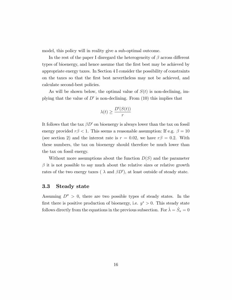
As will be shown below, the optimal value of S(t) is non-declining, im-

plying that the value of D′ is non-declining. From (10) this implies that

λ(t) ≥ D′(S(t))

r

It follows that the tax βD′ on bioenergy is always lower than the tax on fossil

energy provided rβ < 1. This seems a reasonable assumption: If e.g. β = 10

(see section 2) and the interest rate is r = 0.02, we have rβ = 0.2. With

these numbers, the tax on bioenergy should therefore be much lower than

the tax on fossil energy.

Without more assumptions about the function D(S) and the parameter

β it is not possible to say much about the relative sizes or relative growth

rates of the two energy taxes ( λ and βD′), at least outside of steady state.

3.3 Steady state

Assuming D′′ > 0, there are two possible types of steady states. In the

first there is positive production of bioenergy, i.e. y∗ > 0. This steady state

follows directly from the equations in the previous subsection. For λ = Sx = 0

16

we have

x∗ = 0 (11)

u′(y∗) = c′(0) + λ∗ (12)

u′(y∗) = b′(y∗) + βD′(S∗x + βy∗) (13)

λ∗ =1

rD′(S∗x + βy∗) (14)

In the long run, the optimal fossil tax is constant and exactly so high that

fossil energy production is zero. This level of the fossil tax is achieved by

cumulative fossil energy production giving so much carbon in the atmosphere

that discounted future damages are equal to this tax rate. Bioenergy will be

produced at the level that is privately optimal given a tax equal to βD′. The

ratio between this tax and the carbon tax is hence βr.

Since c′(0) < b′(y∗) for y∗ > 0, these equations can only be valid if

βD′ < λ∗, i.e. if rβ < 1. As mentioned above, this seems a reasonable

assumption, and if this inequality holds we hence have a steady state with

positive bioenergy production.

In Appendix A I show that if the initial value of Sx is suffi ciently small,

this steady state is reached asymptotically with monotonically rising values

of λ(t), Sx(t), and S(t).

If rβ > 1 the production of both fossil energy and bioenergy will be zero

in the steady state. Equations (11)-(14) remain valid, except that y∗ = 0,

and = is replaced by < in (13). Notice that even if y∗ = 0, it may be optimal

to have y(t) > 0 for some t. To see this, assume y(t) = 0 for all t. With

positive production of fossil energy λ(t) will be be positive and rising for

D′′ > 0 (see (10)). However, it may well be the case that D′ is small or even

zero for low values of Sx, implying that we may have βD′(S(t)) < λ(t) for

some t even if rβ > 1. But if this is the case it follows immediately from (6)

and (7) that x(t) > 0 and y(t) = 0 cannot be optimal. This contradiction

proves that even if rβ > 1, it may be optimal to have positive production of

17

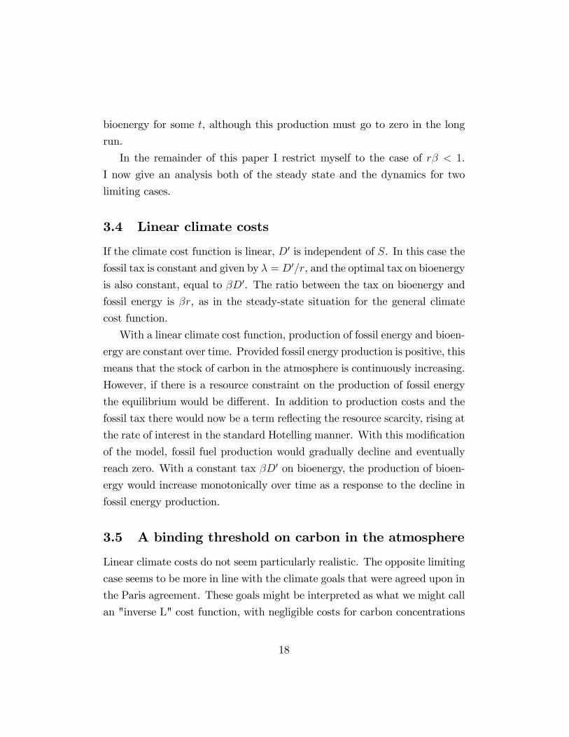
bioenergy for some t, although this production must go to zero in the long

run.

In the remainder of this paper I restrict myself to the case of rβ < 1.

I now give an analysis both of the steady state and the dynamics for two

limiting cases.

3.4 Linear climate costs

If the climate cost function is linear, D′ is independent of S. In this case the

fossil tax is constant and given by λ = D′/r, and the optimal tax on bioenergy

is also constant, equal to βD′. The ratio between the tax on bioenergy and

fossil energy is βr, as in the steady-state situation for the general climate

cost function.

With a linear climate cost function, production of fossil energy and bioen-

ergy are constant over time. Provided fossil energy production is positive, this

means that the stock of carbon in the atmosphere is continuously increasing.

However, if there is a resource constraint on the production of fossil energy

the equilibrium would be different. In addition to production costs and the

fossil tax there would now be a term reflecting the resource scarcity, rising at

the rate of interest in the standard Hotelling manner. With this modification

of the model, fossil fuel production would gradually decline and eventually

reach zero. With a constant tax βD′ on bioenergy, the production of bioen-

ergy would increase monotonically over time as a response to the decline in

fossil energy production.

3.5 A binding threshold on carbon in the atmosphere

Linear climate costs do not seem particularly realistic. The opposite limiting

case seems to be more in line with the climate goals that were agreed upon in

the Paris agreement. These goals might be interpreted as what we might call

an "inverse L" cost function, with negligible costs for carbon concentrations

18

(or temperature) below some threshold, and "infinitely" high costs above the

threshold. Hence, we therefor consider this case below. Assume now that

D′ = 0 for S < S and D′ = ”∞” for S > S. (Our results would not be

changed much if we instead assumed a small and constant marginal cost for

values of S below the threshold S.). The interpretation of D′ for this case is

that it is an endogenous shadow price associated with the constraint S ≤ S.

Provided Sx(0) is small enough, it follows from the monotonicity result

above that the solution will have two phases: First (before t1 in Figure 4)

S(t) < S and rising, and then a phase with S(t) = S.

x

4Figuretime

y

x y+

1t 2t

*y

,x y

Consider first the phase where S(t) < S. In this phase the carbon tax λ(t)

rises at the rate of interest, while the bioenergy tax βD′ is zero. This gives

(from (6) and (7)) a declining x(t), a rising y(t), and a declining x(t) + y(t),

19

as illustrated in Figure 4.

When S(t) reaches its upper limit S, the termD′ becomes positive, reduc-

ing y(t). As long as x(t) is positive, y(t)must be declining, since Sx(t)+βy(t)

is constant during this phase. In Figure 4 this phase lasts till t2, after which

we have the steady-state outcome (x, y) = (0, y∗). (In reality this phase is

reached only asymptotically; i.e. t2 = ”∞”).

The reason we get the "the rise and fall of bioenergy" as illustrated in

Figure 4 is the following. As long as carbon in the atmosphere is below the

threshold, there is no negative climate impact of using bioenergy, and since

its marginal utility increases as fossil energy production declines, the pro-

duction of bioenergy increases. However, once the threshold S is reached,

the production of bioenergy must be reduced to "make room for" the car-

bon released from the fossil energy use. In practise, this comes about by

reconverting land used for bioenergy production to forest land, and from

less intensive harvesting of standing forests, so the volume, and hence stored

carbon, of such forests increases.

4 Second-best policy

Assume that the energy taxes are θx(t) and θy(t), so that an interior market

equilibrium is given by

u′(x(t) + y(t)) = c′(x(t)) + θx(t) (15)

u′(x(t) + y(t)) = b′(y(t)) + θy(t) (16)

As discussed previously, this equilibrium will coincide with the social opti-

mum if the taxes θx(t) and θy(t) are equal to the λ(t) and βD′(S) derived in

section 3. Assume now that, for whatever reason, θx(t) is exogenously set at

a level satisfying

θx(t) <

∫ ∞0

e−rτD′(S(t+ τ))dτ (17)

20

In other words, there is an exogenous carbon tax that is lower than the social

cost of carbon.

For a given time path of y(t), (15) and (16) determine the time path of

x(t) (and of θy(t)). We write this relationship as x = x(y, θx). Choosing

y(t) to maximize our objective function (5) gives the following Hamiltonian

(ignoring the time references):

H = u(x(y, θx) + y)− c(x(y, θx))− b(y)−D(Sx + βy) + (−λ)x(y, θx) (18)

The conditions for an interior optimum are

u′(x+ y) = b′(y) + βD′(S) +

[(λ+ c′ − u′)∂x(y, θx)

∂y

](19)

λ = rλ−D′(S) (20)

Limt→∞e−rtλ(t) = 0 (21)

The costate variable λ(t) may as in the first-best case be interpreted as the

social cost of carbon. From (20) and (21) we can derive

λ(t) =

∫ ∞0

e−rτD′(S(t+ τ))dτ (22)

Define

k = −∂x(y, θx)

∂y(23)

From (15) and (16) it follows that k = u′′

u′′−c′′ , implying that k ∈ (0, 1).

Using the definitions above, it follows from (15) that (19) may be rewrit-

ten as

u′(x+ y) = b′(y) + βD′(S)− k[λ(t)− θx(t)]

Using (16) the second-best optimal tax on bioenergy follows:

θy(t) = βD′(S)− k[λ(t)− θx(t)] (24)

21

To interpret (24), it is useful to rewrite it as θy = βD′(S)−kλ+kθx. The

first term in this expression, βD′(S), measures the direct climate cost of pro-

ducing and using bioenergy. The second term, −kλ, represents the reducedclimate costs from fossil energy caused by the increased use of bioenergy. The

final term, kθx, represent a non-environmental indirect cost of increasing the

use of bioenergy: By increasing the use of bioenergy the use of fossil energy

declines. This reduction gives a social cost (ignoring the climate effect, since

this is taken care of by the second term), since the marginal benefit of using

fossil energy exceeds the marginal cost of supplying it. This difference is due

to the carbon tax, since the carbon tax is identical to the difference between

the user and producer price.

4.1 Steady state

Without any assumptions about the exogenous carbon tax θx(t), we cannot

know whether a steady state exists. Hence, we assume that θx(t) in the long

run is equal to (or approaches asymptotically) a constant value θ∗x. If this is

the case and D′′ > 0 there is a steady state given by

x∗ = 0 (25)

u′(y∗) = c′(0) + θ∗x (26)

u′(y∗) = b′(y∗) + θ∗y (27)

λ∗ =1

rD′(S∗x + βy∗) (28)

θ∗y = rβλ∗ − k[λ∗ − θ∗x] (29)

Since c′(0) < b′(y∗) for y∗ > 0, these equations can only be valid if θ∗y <

θ∗x. From the equations above it is clear that this inequality is identical to

rβ < k + (1 − k)θ∗x/λ∗. For θ∗x < λ∗ the r.h.s. of this inequality is smaller

than 1. Hence the condition for y∗ > 0 is stricter in the second-best case

than in the first-best optimum, and is stricter the larger is the relative fossil

22

tax distortion (i.e. the smaller is θ∗x/λ∗). In the remainder of this section I

assume that the inequality rβ < k + (1 − k)θ∗x/λ∗ holds. In other words, I

only consider cases where bioenergy production is positive in a steady state.

From the equations above we see that the sign of θ∗y is ambiguous. It

is positive (i.e. we have a tax on bioenergy in the long run) if rβ >

k (1− θ∗x/λ∗), and negative (i.e. a subsidy to bioenergy in the long run)if rβ < k (1− θ∗x/λ∗). In other words, with a small carbon tax distortion(θ∗x/λ

∗ close to 1) bioenergy should be taxed in the long run (as in the first-

best case), while bioenergy should be subsidized in the long run if the tax

distortion is suffi ciently high (θ∗x/λ∗ close to 0).

I assumed above that θx(t) in the long run was equal to (or approaches

asymptotically) a constant value θ∗x. Without more assumptions on the time

path of θx(t) is is of course not possible to say anything about the dynamics

toward the steady state. In the next section I shall nevertheless briefly con-

sider the dynamics of the second-best equilibrium for the case of an inverse L

damage function and a particular assumption about the time path of θx(t).

4.2 A binding threshold on carbon in the atmosphere

and a constant parameter of tax distortion.

Assume that the exogenous carbon tax develops in a manner that makes

the variable θx(t)λ(t)

, which is a measure of the tax distortion, constant over

time, denoted α. As in the first-best optimum, the equilibrium will have two

phases. First S(t) < S, and then a phase with S(t) = S.

Consider first the phase where S(t) < S. In this phase the fossil tax αλ(t)

rises at the rate of interest. Since D′ is zero in this phase, it follows from

(24) that θy = −k(1− α)λ. Hence, bioenergy is subsidized, and the subsidy

is increasing over time. This gives a declining x(t) and a rising y(t), as in

the first-best case.

When S(t) reaches its upper limit S, y(t) is declining for x(t) > 0, since

Sx(t)+βy(t) is constant during this phase. This is achieved trough a gradual

23

reduction in the subsidy to bioenergy (as D′ increases), which might even

eventually turn into a tax.

We assumed above that the fossil tax was exogenous and below the level

giving the social optimum. This type of assumption is quite often made

in various studies of second-best climate policies. One reason for such a

constraint on the fossil tax could be distributional concerns. Even if the

government intends to fully recycle the revenues from a carbon tax, each

voter may focus on the visible tax increase and not trust that the revenue

from the carbon tax will be recycled in a way compensating him or her.

Moreover, some persons will be hurt more by the carbon tax than others;

this will typically be those who consume more than the average share of

fossil fuels due to their current preferences or earlier investments (e.g. a

large house with a long commuting distance). On the production side, some

industries will bear a disproportionately high share of the total costs from

the carbon tax. Consumers with a high use of fossil fuels as well as workers

and owners in such high emission sectors will often be successful in lobbying

against a carbon tax.

In contrast, the costs of subsidizing renewable energy are likely to be less

visible to the typical voter and also be more evenly shared by everyone in

the economy. Sectors in the economy producing renewable energy or inputs

to this production will gain from a subsidy to renewable energy, and might

thus engage in lobbying for the use of such subsidies instead of a carbon tax.

These arguments suggest that it might be easier to obtain political support

for a subsidy to renewable energy than for a carbon tax.

Since fossil energy production in the long run is zero, there is no revenue

from the fossil energy tax in the long run. The only purpose of the tax in

the long run is to make it prohibitively expensive to produce fossil energy,

and hence avoid any fossil energy production. In such a situation, it can

obviously not be the fossil tax itself, and the distributional issues related

to the revenue from it, that raises political concerns. There may however

24

be distributional concerns related to the user cost of energy (be it fossil or

bio), and political objections to high energy prices. From (13) it immediately

follows that the long-run energy price u′(y∗) is higher the higher is the fossil

tax θ∗x. Hence, there are political arguments for a constraint on the fossil tax

even if there are no tax revenues collected and redistributed.

5 The climate effects of bioenergy

So far we have assumed Sy = βy, implying that any change in the level of

bioenergy production immediately gives a corresponding change of carbon in

the atmosphere. As mentioned in section 2.2, the change in the amount of

carbon to a new long-run level will not be immediate, and we will instead

get an adjustment as illustrated by the dashed lines in Figure 3.

A simple way to model a gradual adjustment as illustrated by the dashed

lines in Figure 3 would be to assume that Sy(t) develops according to

Sy(t) = δ (βy(t)− Sy(t)) (30)

where δ is a positive parameter.

With this modification it is straightforward to show that (5)-(10) remain

valid with the exception of (7), which is replaced by

u′(x+ y)− b′(y)− γ(t) ≤ 0 [ = 0 for y > 0]

where

γ(t) = δβ

∫ ∞0

e−(r+δ)τD′(S(t+ τ))dτ

25

Notice that

Limδ→∞γ(t) = βD′(S(t))

Limδ→0γ(t) = 0

Hence, if the speed of adjustment is suffi ciently high (large δ), the results

of our model will remain valid. On the other hand, with a very low speed of

adjustment (δ close to zero), production of bioenergy will be almost without

any climate impact, and the optimal tax on bioenergy will be close to zero.

Equation (30) implicitly assumed symmetry, in the sense that carbon

is reduced from the atmosphere when bioenergy production is reduced just

as fast as carbon in the atmosphere is increased when the production of

bioenergy is increased. This is obviously not realistic. Cutting down a forest

to make land available for bioenergy crops will give an immediate release of

carbon to the atmosphere. Converting farm land to forest land will on the

other hand only give a slow growth of carbon contained in the forest.

A limiting case of the asymmetry suggested above would be to replace

Sy(t) = βy(t) with Sy(t) = βmaxτ≤t y(τ). Clearly, with this assump-

tion there will be no climate impact of bioenergy for any t when y(t) <

maxτ≤t y(τ), so that the optimal value of y is then given by u′(x+y) = b′(y).

This implies that we will never have y(t) < 0. To see this, assume y(t) < 0 for

some t. It then follows from u′(x+y) = b′(y) and the fact that x(t) is declining

(due to λ(t) rising) that y(t) must be rising. This contradiction proves that

with the Sy(t) = βmaxτ≤t y(τ), the optimal outcome must satisfy y(t) ≥ 0

for all t. Replacing the assumption Sy(t) = βy(t) with Sy(t) = βmaxτ≤t y(τ)

is hence equivalent to keeping the assumption Sy(t) = βy(t) but adding the

constraint y(t) ≥ 0 for all t.

Assume that without the constraint y(t) ≥ 0 the optimal path of y(t) is

qualitatively as in Figure 4, i.e. that there is a period before the steady state

is reached where y is larger than the steady-state level y∗. This equilibrium is

26

not feasible with the constraint y(t) ≥ 0. One feasible outcome would be to

simply keep y(t) at its steady-state value y∗ once this is reached. Compared

with the unconstrained case, we would then get a loss in social welfare for

the time period when y(t) > y∗ without the constraint. This loss could be

reduced by letting y(t) increase to some value y∗∗ > y∗, as illustrated in

Figure 5. Doing this would come at the cost of a long-run loss in social

welfare, i.e. for all t where we would like to have y(t) < y∗∗ without the

constraint. With a positive discount rate, it is optimal to accept some long-

rune loss in order to make the near-term loss in social welfare smaller. This

intuitive description of the optimum is confirmed by the formal analysis given

in Appendix B.

x

5Figuretime

y

x y+

1t 2t

**y

,x y

27

6 Concluding remarks

In recent years it has become clear that the production of bioenergy in most

cases will have a negative direct climate impact. This suggests that contrary

to what is the case in many countries, bioenergy ought to be taxed, and

certainly not subsidized.

Ideally, all flows of carbon to the atmosphere should be taxed at the

same rate, and this same rate should be used to subsidize flows of carbon

from the atmosphere. For fossil energy this simply implies a uniform carbon

tax, as in this case there is no flow of carbon from the atmosphere to the

biosphere. However, for bioenergy there are generally flows of carbon be-

tween the biosphere and the atmosphere going in both direction. The ideal

tax/subsidy scheme for bioenergy is likely to be diffi cult or impossible to

achieve in practise. In the context of our simple model, the first-best social

optimum may nevertheless be achieved by appropriate taxes on both types of

energy. Due to the differences in dynamics of the climate impact of bioenergy

and fossil energy, the optimal taxes of the two types of energy may have very

different time paths.

If policy makers for some reason are not willing to tax carbon energy as

high as the climate considerations require, it may be optimal to subsidize

bioenergy. However, even if such a such a subsidy is (second-best) optimal

in the short run, it may be optimal to eventually reduce the subsidy and

perhaps tax bioenergy in the long run.

The difference in the dynamics of the climate impacts of bioenergy and

fossil energy have an important implication for the dynamics of the produc-

tion of the two types of energy. Both in the first-best and second-best case

it may be optimal to have an initially rising, but later declining, production

of bioenergy.

The present study has completely ignored the possibility of CCS (Carbon

Capture and Storage). An interesting extension would be to include the

possibility of CCS, both in a first-best and second-best setting.

28

Appendix A: The dynamics towards steady state.

For an interior solution it follows from (6) and (7) and the properties of the

functions that

x = x(λ−, Sx)+

(31)

y = y(λ+, Sx)−

(32)

It follows that

S = Sx + βy(λ, Sx) = S(λ+, Sx)+

(33)

To see that S is increasing in Sx, assume the opposite. Then it would follow

from (6) and (7) that an increase in Sx for given λ would make y higher or

unchanged, and hence increase S. This contradiction proves the last sigh in

(33)

The phase diagram in Figure 6 follows from (3) and (8). From (3) and

(31) it is clear that the line for x(λ, Sx) = 0 is upward sloping, and that Sxis zero above this line and positive below.

When λ = 0 it follows from (8) that

λ =1

rD′(Sx + βy(λ, Sx))

When x = 0 it follows from (7) that y is independent of λ, and since S and

D′ is higher the higher is Sx, the curve for λ = 0 must be upward sloping

above the line for x(λ, Sx) = 0. The slope below this line is not obvious, but

is of no importance. In any case we must have λ = rλ−D′(S(λ, Sx)) > 0 to

the left of the curve giving λ = 0.

If the initial value of Sx is higher than the steady-state value S∗x, the

optimal solution is trivial: We should have x = 0 for all t,and y constant and

determined by (7) for all t.

29

If the initial value of Sx is lower than the steady-state value S∗x, as in

Figure 6, the dynamics are as illustrated: Sx(t) and λ(t), and hence also S(t),

rise monotonically and asymptotically towards their steady-state values.

0λ =&

6Figure( )xS t

+

( )tλ

0xS =&

*xS(0)xS

−

+0

*λ

(0)λ

Appendix B: Non-declining bioenergy produc-

tion

Consider the same problem as in Section 3.1, but now with the additional

constraint y(t) ≥ 0. To analyze this problem, I treat y(t) as a state variable

30

and add a control variable w(t), with the relationship between the two being

y(t) = w(t). Moreover, we have the constraint that w(t) ≥ 0.

The current value Hamiltonian is now (ignoring time references and writ-

ten so the costate variables λ and σ are non-negative)

L = u(x+ y)− c(x)− b(y)−D(Sx + βy) + (−λ)x+ (−σ)w

Ignoring a possible initial jump upwards in y (with w being "very large" for

a "very short" time), the conditions for an interior optimum are now

u′(x+ y)− c′(x)− λ = 0 (34)

σ ≥ 0 [ = 0 for w > 0] (35)

λ = rλ−D′(S) (36)

σ = rσ + [u′ − b′ − βD′] (37)

Limt→∞e−rtλ(t) = 0 (38)

Limt→∞e−rtσ(t) = 0 (39)

It is immediately clear that x(t) is determined as before by (6) and (10),

i.e. u′(x+ y) = c′(x) +λ, where λ is the social cost of carbon. Hence, also in

this case x is monotonically declining.

The exact equilibrium for y(t) will depend on the function D(S). If the

equilibrium without the constraint y ≥ 0 never has y < 0 (e.g. as in the

case of D′′ = 0), the constraint y ≥ 0 is non-binding. In this case we will

have σ(t) = 0 for all t, and the conditions above give the same outcome as

in Section 3.1.

The interesting case is when it is optimal to have y(t) < 0 for some t in the

unconstrained case. For this case, the optimal solution for the constrained

case has three phases (or only two, see below).

In the first phase y(t) is increasing and σ(t) = 0. From the equations

31

above this implies that y is determined as before by (7), i.e. u′(x + y) =

b′(x) + βD′(S). In the second phase y is constant and σ > 0. The phase

starts with y being constant and u′(x+ y)− b′(y)− βD′(S) rising from zero

due to x declining. From (37) this implies that σ will start to rise. Initially,

σ > rσ. However, as D′ rises due to the increasing S, the term in brackets

in (37) will eventually become negative, making σ < rσ . This phase ends

when σ stops growing so that its steady state σ∗∗ is reached. From then on

we are in phase three with x = 0 and

u′(y∗∗) = b′(y∗∗) + βD′(S∗∗)− rσ∗∗ (40)

Four properties of the equilibrium are worth mentioning. First, the exis-

tence of the first phase depends on the initial conditions; if e.g. the initial

amount of fossil carbon in the atmosphere is suffi ciently high we would only

get the two last phases.

Second, the equilibrium described above relied on u′(x+y)−b′(y)−βD′(S)

changing from positive to negative as S increased. This will only occur if D

is suffi ciently convex. If D doses not have this property, the equilibrium will

be unaffected by the constraint y(t) ≥ 0, as explained above.

Third, the third phase will generally only be reached asymptotically.

However, with an inverse L damage cost function, a constant y and u′(x+y) =

c′(x) + λ must imply that x is reached in finite time since λ = rλ as long as

the threshold S has not been reached.

Finally, it is clear that the steady-state value y∗∗ given by (40) is larger

than the corresponding value y∗ in the unconstrained case (since σ∗∗ > 0).

The intuition of this result is explained in the main text.

32

References

Amundsen, E. and J. B. Mortensen (2001). The Danish Green CertificateSystem: some simple analytical results. Energy Economics, 23 , 489—509.

Archer, D. (2005). Fate of fossil fuel CO2 in geologic time. Journal ofGeophysical Research, 110 , C09S05.

Chakravarty, U., M. Hubert and L. Nostbakken (2009). Fuel versus food.Annual Review of Resource Economics, 1 , 545—663.

Chakravorty, U. and M. Hubert (2013). Global impacts of the biofuel man-date under a carbon tax. Americal Journal of Agricultural Economics, 95 ,282—288.

Chakravorty, U., B. Magne and M. Moreaux (2008). A dynamic model offood and clean energy. Journal of Economic Dynamics & Control , 32 (4),1181—1203.

Crutzen, P., A. Mosier, K. A. Smith and W. Winiwarter (2008). N2O releasefrom agro-biofuel production negates global warming reduction by replacingfossil fuels. Atmospheric Chemistry and Physics, 8 , 389—395.

De Gorter, H. and D. Just (2009). The economics of a blend mandate forbiofuels. American Journal of Agricultural Economics, 91 , 738—750.

De Gorter, H. and D. Just (2010). The Social Cost and Benefits of Biofuels:The Intersection of Environmental, Energy and Agricultural Policy. AppliedEconomic Perspectives and Policy, 32 , 4—32.

Eggert, H. and M. Greaker (2012). Trade policies for biofuels. Journal ofEnvironment and Development , 21 , 281—306.

Fargione, J., J. Hill, D. Tilman, S. Polasky and P. Hawthorne (2008). Landclearing and the biofuel carbon dept. Science, 319 , 1235—1238.

Fischer, C. and S. Salant (2012). Alternative Climate Policies and Intertem-poral Emissions Leakage: Quantifying the Green Paradox. Working Paper12-16, Resources for the Future.

33

Grafton, R. Q., T. Kompas and N. V. Long (2012). Substitution between Bio-fuels and Fossil Fuels: Is there a Green Paradox? Journal of EnvironmentalEconomics and Management , 64 (3), 328—341.

Greaker, M., M. Hoel and K. E. Rosendahl (2014). Does a Renewable FuelStandard for Biofuels Reduce Climate Costs? Journal of the Association ofEnvironmental and Resource Economists, 1 , 337—363.

Hill, J., E. Nelson, D. Tilman, S. Polasky and D. Tiffany (2006). Environ-mental, economic, and energetic costs and benefits of biodiesel and ethanolbiofuels. Proceedings of the National Academy of Sciences of the United Statesof America, 103 (30), 11206—11210.

Hoel, M., B. Holtsmark and K. Holtsmark (2014). Faustmann and the Cli-mate. Journal of Forest Economics, 20 , 192—210.

Hoel, M. and T. M. Sletten (2016). Climate and forests: The tradeoffbetweenforests as a source for producing bioenergy and as a carbon sink. Resourceand Energy Economics, 43 , 112—129.

Lapan, H. and G. Moschini (2010). Second-best biofuel policies and thewelfare effects of quantity mandates and subsidies. Journal of EnvironmentalEconomics and Management , 63 , 224—241.

Lapola, D. M., R. Schaldach, J. Alcamo, A. Bondeau, J. Koch, C. Koelkingand J. A. Priess (2010). Indirect land-use changes can overcome carbonsavings from biofuels in Brazil. PNAS , 107 , 3388—3393.

Macedo, I. C., J. Seabra and J. Silva (2008). Greenhouse gas emissions inthe production and use of ethanol from sugarcane in Brazil: The 2005/2006averages and a prediction for 2020. Biomass and Energy, 32 , 582—595.

Millner, A. (2015). Policy distortions due to heterogeneous beliefs: Somespeculative consequences for environmental policy. In Schneider, A. K., Fand J. Reichl (eds.), Political Economy and Instruments of EnvironmentalPolitics. MIT Press.

Searchinger, T., R. Heimlich, R. Houghton, F. Dong, A. Elobeid, J. Fabiosa,S. Tokgoz, D. Hayes and T.-H. Yu (2008). Use of U.S. Croplands for Biofu-els Increases Greenhouse Gases Through Emissions from Land-Use Change.Science, 319 , 1238—1241.

34

Tahvonen, O. (1995). Net national emissions, CO2 taxation and the role offorestry. Resource and Energy Economics, 17 , 307—315.

van Kooten, C., C. Binkley and G. Delcourt (1995). Effect of Carbon Taxesand Subsidies on Optimal Forest Rotation Age and Supply of Carbon Ser-vices. American Journal of Agricultural Economics, 77 , 365—374.

35