the riemann and extrinsic curvature tensors...
TRANSCRIPT
Class.Q.Grav. Vol.5(1988) pp.1193-1204 25-May-1987
THE RIEMANN AND EXTRINSIC CURVATURE TENSORS
IN THE REGGE CALCULUS
Leo Brewin†
Department of Physics
University of British Columbia
British Columbia, V6T 2A6
Canada
A detailed analysis of the Riemann tensor in the neighbourhood of one bone and of the
extrinsic curvature in the neighbourhood of one triangular face in a simplicial geometry is
presented. Unlike most previous analyses this analysis makes no reference to any particular
choice of smoothing scheme. Explicit formulae will be presented for both the Riemann
and extrinsic curvature tensors. These results are applied, using the formalism developed
in an earlier paper [1] , in deriving an exact formula for the integral extrinsic curvature.
It is argued that for integrals of R2, R3 · · · contributions must be expected from the legs,
vertices,... rather than just from the bones. This work provides the background material for
the following paper in which the Gauss-Codacci equation is applied to a Regge spacetime.
† Present address : Department of Mathematics
Monash University
Clayton, Vic. 3168
Australia
2
1. Introduction.
This is the first of two papers dealing with certain aspects of the Riemann and extrinsic
curvature tensors on a Regge spacetime. The basic aim is to produce a “3+1” formulation
of the Regge calculus.
In an earlier paper [1] a first order continuous time formulation of the Regge calculus was
developed. Unfortunately the evolution equations presented in that paper made reference
to the defects in the full 4-dimensional spacetime. If a “3+1” formulation is to be achieved
then it will be necessary to develop an expression for those defects in terms of the defects
on each leaf and of the extrinsic curvature of the foliation. It is our aim to present such a
relationship in this pair of papers.
In this paper the basic expression for the Riemann and extrinsic curvature tensors will
be presented. In the following paper these results will be employed in the development
of the Gauss-Codacci equation. It is from this expression that the relation linking the
4-defects with the 3-defects will be obtained.
Many authors [2,3,4,5,6,7,8,9] have previously provided derivations of the Riemann tensor
for simplicial geometries. In each of these papers the authors made one or more of the
following assumptions,
i) that the simplicial geometry may be explicitly approximated by a parameterized family of
smooth geometries,
ii) that the final expression for the Riemann tensor does not depend upon the choice of that
family,
iii) that the defect for a finite loop equals the sum of the defects for each of the infinitesimal
loops that make up that loop and
iv) that there is no interaction amongst neighbouring bones.
The last three assumptions are, arguably, the most important. The second assumption is
necessary when an explicit choice has been made for the smooth metric. It is quite possible
that the global properties of a singular metric may well depend upon the internal structure
of the singularity (see [10] ). The third assumption arises when formulae familiar from
continuum differential geometry are employed. For example, the change in a vector when

3
parallel transported around an infinitesimal loop is just a small rotation of that vector in
some plane. From this it is argued that the Riemann tensor is proportional to the defect for
this infinitesimal loop. However in the discrete geometry the defect must be calculated for a
finite loop drawn in the far flat regions. It is at this point that the third assumption is made.
The fourth assumption, that there is no interaction between neighbouring bones, allows one
to write, for example, the Hilbert action as a sum over each of the bones. It will be shown
in the last section § 6 that interactions between neighbouring bones must be expected.
The fundamental result, that the Hilbert and Regge actions are equal, can be no more valid
than each of the above assumptions. It is therefore important to try to remove some of these
assumptions. In this paper the last three assumptions will not be required.
There are only a handful of published papers [11,12,13,14,15,16] in which the extrinsic
curvature tensor for a simpilcial spacetime is discussed. The works of Porter [11,12] and
that of Williams [13] contain some approximate expressions for particular components of
Kµν . They obtain their expressions by identifying certain terms in the Regge field equations.
They do not, however, provide any general expression for all of the components of Kµν . Such
an expression is provided by Piran and Williams [14] and also by Friedmann and Jack [15] .
The method employed in both of these papers is based upon the construction of analogies
between the structure of certain tensor fields on a smooth spacetime and of those same fields
on a Regge spacetime. They first develop an analogy for the metric tensor. They then
develop analogies for the first time derivative of the metric, the lapse function and the shift
vectors. This leads directly to an expression for the Kµν .
The main difficulty with this approach is that there is no unique construction for the shift
vectors. Its not surprising then that the results of the two papers are not identical. In this
paper a well defined expression for the Kµν will be obtained by applying the usual formulae
to a family of smooth spacetimes.

4
2. Preliminaries.
Consider a general discrete time “3+1” Regge spacetime [1,17] and focus attention on the
4-dimensional region surrounding one timelike bone. This will consist of the set of worldtubes
adjacent to the bone and the (portions of the) pair of leaves that these worldtubes join. Each
worldtube has a tetrahedral cross section and their intersections with the two leaves are just
the various tetrahedra of those leaves. In the following analysis this sub-region will be treated
as if it where the whole spacetime.
Our aim is to compute the Riemann and extrinsic curvature tensors for this simple spacetime.
However as the metric and the embedding of the leaves in the spacetime need not be smooth
one can not apply the usual formulae. The approach to be adopted here is the usual technique
of applying the formulae to a continuous family of smooth spacetimes and then developing
a suitable limiting procedure. It will therefore be necessary to view the final results as
distributions rather than as ordinary functions.
Let M represent the spacetime, Ti, i = 1, 2, 3... the various worldtubes and Sx
, Sy
the upper
and lower leaves. The various tetrahedra of the leaves will be denoted by sx
i, sy
i, i = 1, 2, 3....
Suppose that sy
i and sy
j are a pair of adjacent tetrahedra in Sy
. Then their triangular
interface will be denoted by sy
ij . The timelike bone will be represented by σ. Its image
in Sy
will be denoted by σ′ and will represent the spacelike bone of Sy
(this is also the
spacelike leg in Sy
upon which σ stands). (Notice that these definitions differ from those
used in Brewin [1,17] .)
5
3. The metric.
Let the smooth family of metrics be denoted by gµν and let the associated smoothing pa-
rameter be #g. The limiting form of gµν as #g → 0 will be the original discrete metric of
M . Now in any Regge spacetime any vector that is parallel to the bone will suffer no change
when parallel transported around any loop. The gµν will be chosen so as to preserve this
symmetry. Thus it is always possible to choose two vectors, pµ and qµ, such that
gµν = gµν + pµpν − qµqν (3.1a)
with
pµ;ν = qµ;ν = 0 . (3.1b)
The two dimensional metric gµν is the metric of the 2-dimensional sheet that is perpendicular
to the bone σ. This sheet will be denoted by C. The metric on C is of Euclidian signature
and will, as #g → 0, be flat everywhere except at the point where C intersects the bone.
The vectors pµ and qµ will be chosen so that pµ is parallel to σ′.
The “3+1” decomposition of the metric is normally written as
gµν = hµν − nµnν (3.2a)
where nµ is the unit timelike normal to Sy
and hµν is the induced (smooth) 3-metric on Sy
.
Notice that nµ may be smoothed independently of gµν . The associated smoothing parameter
will be represented by #n. Notice also that since nµ = gµνnν it will be necessary to view
the nµ as being dependent on both #g and #n. Now since pµ is parallel to σ′ it is possible
to write
hµν = hµν + pµpν (3.2b)
for some 2-metric hµν . This 2-metric represents the metric of some 2-dimensional sheet
which, in general, will not coincide with C. This sheet will be represented by C ′.
6
4. The Riemann tensor.
The form of the metric in (3.1a,b) leads to an immediate simplification in the computation
of the Riemann tensor, namely
Rµναβ(g) = Rµ
ναβ(g) .
Now consider a small rectangle, drawn in C, and generated by the two vectors δxµ1 and δxµ2 .
Suppose vµ is any vector lying in the tangent space to C. When vµ is parallel transported
around this loop the net change in vµ will be equivalent to a rotation of vµ through some
small angle – the defect angle. Denote this angle by δα. It follows that
δvµ =
(
δα
δA
)
Uµν v
ν δA
where Uµν is the bivector of C and δA is the area of the loop. Now by writing
δA = Uαβ δxα1 δx
β2
it is easy to see that the components of the Riemann tensor are given by
Rµναβ(g) = d(g)Uµ
νUαβ (4.1)
where d(g) = δα/δA is the defect per unit area on C. This is the fundamental form of
the Riemann tensor for one timelike bone. Quite clearly the limit lim#g→0 d(g) does not
exist as a well defined ordinary function (the limit diverges for points on σ yet it vanishes
everywhere else). The correct approach would be to view the limit as a generalized function.
Thus lim#g→0 d(g) will be viewed as a Dirac distribution, with respect to the measure√−g,
with compact support on σ.
An important property of the defects for various small loops on C is that they are additive.
That is, the net defect for a loop composed of a number of smaller loops is just the sum
of the defects for the individual loops. This may be proved as follows. Denote the loop by
L and let this loop be composed of the smaller loops Li, i = 1, 2, 3.... Suppose the defects

7
associated with these loops are θ and θi respectively. Similarily let Uµν and Uµνi be the
associated bivectors. The Bianchi identities for this set of loops may be written as
exp(θUµν) =
∏
i
exp(θUµν)i .
But since each of the components of Uµν and Uµνi are equal (which may be proved by noting
that Uµν is tangent to C and pµ;ν = qµ;ν = 0 thus Uµν;α = 0) it is clear that the Bianchi
identities may be reduced to
θ =∑
i
θi
which proves the assertion.
Now imagine that the loop L is chosen as some large loop in the almost flat far regions of
C and that each of the Li is an infinitesimal loop. Then the θ of L will, as #g → 0, be
just the defect α of the original discrete spacetime M . Each of the θi may be accurately
approximated by d(g)δ2Ai where δ2Ai is the area of the loop Li. Thus it follows that the
above relation may be reduced, as #g → 0, to
α = lim#g→0
∫
Cd(g)
√
g d2x . (4.2)
This result establishes the link between the global defect of the discrete geometry and the
local defect of the smooth geometry. Combining (4.1) and (4.2) leads directly to
lim#g→0
∫
MR√−g d4x = 2αA (4.3)
where A is the area of σ. This particular result is not new but the method employed, which
avoids the use of any specific smoothing schemes, is new (cf. [5] ).
It is rather easy to see that this same method may also be applied to any spacelike bone.
However in this instance the geometry of C is hyperbolic rather than Euclidian.

8
5. The Extrinsic curvature tensor.
The extrinsic curvature tensor is normally defined by
Kµν = nµ;ν (5.1)
where nµ is the unit tangent vector to the geodesics normal to Sy
. On the interior of any one
tetrahedron the Kµν must vanish. However at the various interfaces between neighbouring
tetrahedra the Kµν when viewed as ordinary functions must be singular. By introducing
a smoothing scheme for the embedding of Sy
in M it is possible to re-interpret Kµν as
a generalized function in the neighbourhoods of the triangular interfaces. However the
behaviour of the Kµν in the neighbourhood of the bone σ′ of S
y
depends crucially upon the
smoothing scheme. Consequently the following analysis will apply only to the neighbourhood
of a typical triangular interface in Sy
.
Consider a typical pair of adjacent tetrahedra sy
1 and sy
2 of Sy
. Denote the triangular
interface between this pair by sy
12. Now consider some arbitrary path Γ(w), parameterized
by the proper distance w, joining some point P in sy
1 to some point Q in sy
2. Along Γ
the normal nµ is a well defined vector field varying smoothly with w. If nµ at P is parallel
transported to some intermediate point on Γ then it will be related to the actual nµ at that
point by a rotation, through some angle β, in a plane perpendicular to sy
12. The angle β
will, when both #g and #n are sufficiently small, depend only upon the distance measured
away from the interface sy
12 (ie. in the discrete space nµ changes only upon crossing the
interface).
The change in nµ arising from the parallel transportation of nµ along Γ will, therefore, be
given by
δnµ = (δβ)Wµνn
ν = nµ;ν δxν
where Wµν is the bivector of the 2-dimensional plane in Sy
and perpendicular to sy
12.
However
δβ =δβ
δstα δx
α

9
where s is the proper distance measured along the geodesic normal to sy
12 in Sy
and tα is
the unit tangent to that geodesic. Combining this expression, the previous expression and
(5.1) leads to
Kµν =
(
δβ
δs
)
Wµαn
αtν .
By choosing
Wµν = nµtν − tµnν
as a representation for Wµν the previous expression may be reduced to
Kµν =
(
δβ
δs
)
tµtν . (5.2)
This is the fundamental form of the extrinsic curvature tensor for a triangle sy
jk in Sy
. As
with d(g), the quantity δβ/δs is best viewed as a Dirac distribution with support on sy
jk as
#g,#n → 0.
Two important steps remain, firstly to identify the strength of this Dirac distribution and,
secondly to then express that strength in terms of the Cauchy data of a “3+1” formulation.
The first step will be achieved by evaluating a volume integral of K = Kµµ. For the second
step the formalism developed in a recent paper [17] will be used.
The trace of the extrinsic curvature is
K =δβ
δs. (5.3)
Now choose any 3-dimensional region Ωjk in Sy
that contains sy
jk but does not contain any
points of σ′. The integral of K throughout this region is
∫
Ωjk
K√h d3x =
∫
Ωjk
δβ
δs
√h d3x .
The volume element in the right hand integral may be written as dsd2B where d2B is the
element of area of sy
jk and s is the distance measured normal to sy
jk. As #g,#n are
reduced to zero the integral in ds is constant over sy
jk.
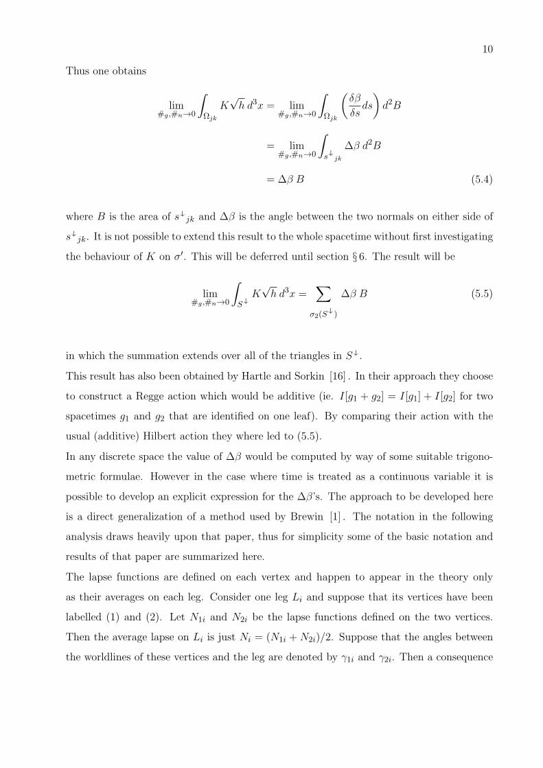
10
Thus one obtains
lim#g,#n→0
∫
Ωjk
K√h d3x = lim
#g,#n→0
∫
Ωjk
(
δβ
δsds
)
d2B
= lim#g,#n→0
∫
sy
jk
∆β d2B
= ∆β B (5.4)
where B is the area of sy
jk and ∆β is the angle between the two normals on either side of
sy
jk. It is not possible to extend this result to the whole spacetime without first investigating
the behaviour of K on σ′. This will be deferred until section § 6. The result will be
lim#g,#n→0
∫
Sy
K√h d3x =
∑
σ2(Sy
)
∆β B (5.5)
in which the summation extends over all of the triangles in Sy
.
This result has also been obtained by Hartle and Sorkin [16] . In their approach they choose
to construct a Regge action which would be additive (ie. I[g1 + g2] = I[g1] + I[g2] for two
spacetimes g1 and g2 that are identified on one leaf). By comparing their action with the
usual (additive) Hilbert action they where led to (5.5).
In any discrete space the value of ∆β would be computed by way of some suitable trigono-
metric formulae. However in the case where time is treated as a continuous variable it is
possible to develop an explicit expression for the ∆β’s. The approach to be developed here
is a direct generalization of a method used by Brewin [1] . The notation in the following
analysis draws heavily upon that paper, thus for simplicity some of the basic notation and
results of that paper are summarized here.
The lapse functions are defined on each vertex and happen to appear in the theory only
as their averages on each leg. Consider one leg Li and suppose that its vertices have been
labelled (1) and (2). Let N1i and N2i be the lapse functions defined on the two vertices.
Then the average lapse on Li is just Ni = (N1i +N2i)/2. Suppose that the angles between
the worldlines of these vertices and the leg are denoted by γ1i and γ2i. Then a consequence
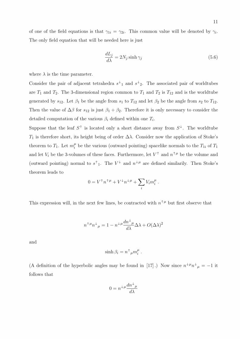
11
of one of the field equations is that γ1i = γ2i. This common value will be denoted by γi.
The only field equation that will be needed here is just
dLj
dλ= 2Nj sinh γj (5.6)
where λ is the time parameter.
Consider the pair of adjacent tetrahedra sy
1 and sy
2. The associated pair of worldtubes
are T1 and T2. The 3-dimensional region common to T1 and T2 is T12 and is the worldtube
generated by s12. Let β1 be the angle from s1 to T12 and let β2 be the angle from s2 to T12.
Then the value of ∆β for s12 is just β1 + β2. Therefore it is only necessary to consider the
detailed computation of the various βi defined within one Ti.
Suppose that the leaf Sx
is located only a short distance away from Sy
. The worldtube
T1 is therefore short, its height being of order ∆λ. Consider now the application of Stoke’s
theorem to T1. Let mµi be the various (outward pointing) spacelike normals to the T1i of T1
and let Vi be the 3-volumes of these faces. Furthermore, let Vx
and nx
µ be the volume and
(outward pointing) normal to sx
1. The Vy
and ny
µ are defined similarily. Then Stoke’s
theorem leads to
0 = Vx
nx
µ + Vy
ny
µ +∑
i
Vimµi .
This expression will, in the next few lines, be contracted with nx
µ but first observe that
nx
µny
µ = 1− ny
µdny
µ
dλ∆λ+O(∆λ)2
and
sinh βi = nx
µmµi .
(A definition of the hyperbolic angles may be found in [17] .) Now since ny
µny
µ = −1 it
follows that
0 = ny
µdny
µ
dλ

12
and consequently the contracted form of the above equation may be reduced to
0 = −∆V +∑
i
∆Vi sinh βi +O(∆λ)2
where ∆V = Vx
−Vy
and ∆Vi is the small value of Vi. The ∆Vi will be computed, accurate
to O(∆λ)2, as the product of the area of the base sy
1i with the average height of T1i. Denote
by ∆h(x)i the distance measured from the point x in s1i along the geodesic normal to s1i
in T1i (see Fig(1)). Let ∆hi be the average of ∆h(x)i over s1i and let Bi be the area of s1i,
then
∆Vi = Bi∆hi +O(∆λ)2
Now since ∆h(x)i is a linear function over s1i its average may be expressed as
∆hi =1
3
∑
j
∆hij
where ∆hij is the average of ∆h(x)i over each of the legs of s1i and the sum includes each
leg of s1i. The ∆hij associated with the leg Lj of T1i can be computed by projecting ∆hij
onto the timelike face generated by Lj . Thus if φij is the angle from this face to the base
s1i then
∆hij = Nj cosh γj coshφij∆λ .
In reference [1] it was shown that
sinhφij =2
Lj
∂Bi
∂Ljtanh γj
from which the coshφij may be easily obtained. Upon combining the above expressions one
finds that
∆V =∑
i
∑
j(i)
Bi
3Nj cosh γj coshφij sinh βi∆λ
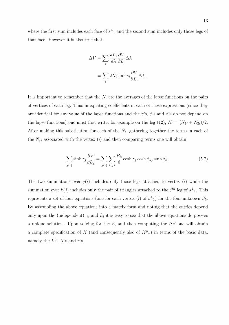
13
where the first sum includes each face of sy
1 and the second sum includes only those legs of
that face. However it is also true that
∆V =∑
i
dLi
dλ
∂V
∂Li∆λ
=∑
i
2Ni sinh γi∂V
∂Li∆λ .
It is important to remember that the Ni are the averages of the lapse functions on the pairs
of vertices of each leg. Thus in equating coefficients in each of these expressions (since they
are identical for any value of the lapse functions and the γ’s, φ’s and β’s do not depend on
the lapse functions) one must first write, for example on the leg (12), Ni = (N1i + N2i)/2.
After making this substitution for each of the Ni, gathering together the terms in each of
the Nij associated with the vertex (i) and then comparing terms one will obtain
∑
j(i)
sinh γj∂V
∂Lj=
∑
j(i)
∑
k(j)
Bk
6cosh γj coshφkj sinh βk . (5.7)
The two summations over j(i) includes only those legs attached to vertex (i) while the
summation over k(j) includes only the pair of triangles attached to the jth leg of sy
1. This
represents a set of four equations (one for each vertex (i) of sy
1) for the four unknown βk.
By assembling the above equations into a matrix form and noting that the entries depend
only upon the (independent) γi and Li it is easy to see that the above equations do possess
a unique solution. Upon solving for the βi and then computing the ∆β one will obtain
a complete specification of K (and consequently also of Kµν) in terms of the basic data,
namely the L’s, N ’s and γ’s.
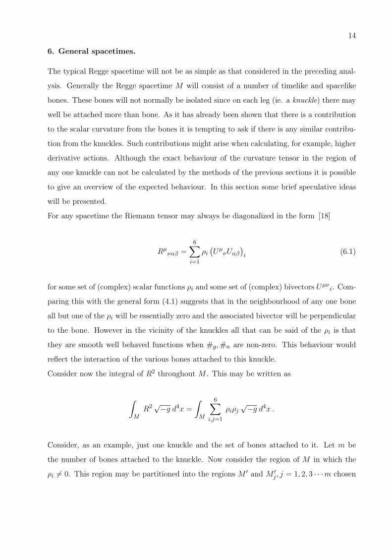
14
6. General spacetimes.
The typical Regge spacetime will not be as simple as that considered in the preceding anal-
ysis. Generally the Regge spacetime M will consist of a number of timelike and spacelike
bones. These bones will not normally be isolated since on each leg (ie. a knuckle) there may
well be attached more than bone. As it has already been shown that there is a contribution
to the scalar curvature from the bones it is tempting to ask if there is any similar contribu-
tion from the knuckles. Such contributions might arise when calculating, for example, higher
derivative actions. Although the exact behaviour of the curvature tensor in the region of
any one knuckle can not be calculated by the methods of the previous sections it is possible
to give an overview of the expected behaviour. In this section some brief speculative ideas
will be presented.
For any spacetime the Riemann tensor may always be diagonalized in the form [18]
Rµναβ =
6∑
i=1
ρi(
UµνUαβ
)
i(6.1)
for some set of (complex) scalar functions ρi and some set of (complex) bivectors Uµνi. Com-
paring this with the general form (4.1) suggests that in the neighbourhood of any one bone
all but one of the ρi will be essentially zero and the associated bivector will be perpendicular
to the bone. However in the vicinity of the knuckles all that can be said of the ρi is that
they are smooth well behaved functions when #g,#n are non-zero. This behaviour would
reflect the interaction of the various bones attached to this knuckle.
Consider now the integral of R2 throughout M . This may be written as
∫
MR2√−g d4x =
∫
M
6∑
i,j=1
ρiρj√−g d4x .
Consider, as an example, just one knuckle and the set of bones attached to it. Let m be
the number of bones attached to the knuckle. Now consider the region of M in which the
ρi 6= 0. This region may be partitioned into the regions M ′ and M ′j , j = 1, 2, 3 · · ·m chosen

15
so that M ′ is a thin tube enclosing the knuckle and the M ′j are thin slabs that enclose the
jth bone on the knuckle. The above integral may then be rewritten as
∫
MR2√−g d4x =
∫
M ′
6∑
i,j=1
ρiρj√−g d4x+
m∑
j=1
∫
M ′
j
6∑
i=1
ρ2i√−g d4x.
Let ρ be an estimate of the average of all of the ρi over all of the points in M ′. Similarily,
let ρj be an estimate of the average of all of the ρi throughout M′j . Let V (M ′) and V (M ′
j)
be the 4-volumes of M ′ and M ′j respectively. Then it follows that as #g → 0
V (M ′) ∼ L#3g
V (M ′j) ∼ Aj#
2g
where L is the length of the knuckle and Aj is the area of the bone inside M ′j . Since the
volume integral of R is known to be finite as #g → 0 it follows that
ρj ∼ #−2g
for each bone. Suppose that on the knuckle
ρ ∼ #−ng
for some unknown integer n. Using these estimates the above relation may be estimated as
∫
MR2√−g d4x ∼ L ·#−2n ·#3 +
m∑
j=1
Aj ·#−4 ·#2 .
If the right hand side is to remain finite as #g → 0 then n = 2.5. A similar analysis could
be used in estimating the behaviour of the ρi for higher powers of R. For R3 it would be
necessary to expect contributions from the vertices as well as the knuckles and bones of M .
Since n = 2.5 is necessary if the volume integral of R2 is to be finite it follows that for the
volume integral of R the contribution from the knuckle behaves like #1/2 and thus vanishes

16
as #g → 0. A direct consequence of this result is that for any well behaved function f over
M
lim#g→0
∫
Mf(x)R
√−g d4x = 2
∑
σ(M)
(fαA)σ
where f is the average of f over a bone and the summation extends over all of the bones in
the spacetime. This shows that for the Hilbert action integral, in which f = 1 throughout
M , one may proceed as if there were no interactions between neighbouring bones. This result
has been used by many other authors but without consideration of the contributions from
the knuckles and vertices.
A similar diagonalization may be used for the Kµν . Thus
Kµν =
3∑
i=1
τi (tµtν)i (6.2)
where the tµi are a particular set of unit orthogonal spatial vectors. In the vicinity of any
triangle all but one of the τi will be essentially zero and the associated tµi will be perpendicular
to that interface. It has already been argued that the functional form of the τi in the vicinity
of the interfaces between the triangles (ie. the knuckles) may be rather complicated. However
there are some important non-linear combinations of the Kµν that will require a detailed
knowledge of the τi in these regions. For example the combination
(Kµµ)
2 −KµνK
νµ =
∑
i 6=j
τiτj
is essentially non-zero only on the knuckles. Presumably this expression may be interpreted
as some distribution with support on the legs of the leaves. Such an interpretation may be
presented in a future paper.
Using techniques similar to that just presented it is not hard to show that contributions to
the integral of, for example, K2 may arise from the knuckles. If that integral is finite then it
follows that there will be no contributions from the knuckles in computing the integral of K
17
and that the simple result (5.4) may be immediately generalized to the result (5.5) of Hartle
and Sorkin [16] .
7. Acknowledgements.
I would like to thank Bill Unruh for his helpful suggestions. This work was completed under
NSERC grant 580441 for Bill Unruh.
18
References.
[1] Brewin, L.,
A continuous time formulation of the Regge calculus.
Class.Quantum Grav. Vol.5(1988)pp.839-847
[2] Regge, T.,
General Relativity without coordinates.
Il Nuovo Cimento. Vol.XIX(1961)pp.558-571.
[3] Wheeler, J.A.,
Geometrodynamics and the issue of the final state.
In Relativity, Groups and Topology edited by C. DeWitt and B. DeWitt, (Gordon and
Breach, New York, 1964).
[4] Cheuk-Yin Wong,
Application of Regge Calculus to the Schwarzschild and Reissner-Nordstrøm geometries at
the moment of time symmetry.
J.Math.Phys. Vol.12(1971)pp.70-78.
[5] Sorkin, R.,
The time evolution problem in the Regge calculus.
Phys.Rev.D Vol.12(1975)p.385.
[6] Sokolov, D.D. and Starobinskii, A.A.,
The structure of the curvature tensor at conical singularities.
Sov.Phys.Dokl. Vol.22(1977)pp.312-314.
[7] Rocek, M. and Williams, R.M.,
Introduction to Quantum Regge Calculus.
In Quantum structure of space and time., ed. M.J. Duff and C.J. Isham, (Cambridge Uni-
versity Press, 1982)pp.105-116.
[8] Friedberg, R. and Lee, T.D.
Derivation of Regge’s action from Einstein’s theory of General Relativity.
Nulc.Phys.B Vol.242(1984)pp.145-166.
19
[9] Hamber, H.W. and Williams, R.M.,
Higher derivative quantum gravity on a simplicial lattice.
Nucl.Phys.B Vol.248(1984)pp.392-414.
[10] Geroch, R. and Traschen, J.,
Strings and other distributional sources in General Relativity.
Phys.Rev.D Vol.36(1987)pp.1017-1031.
[11] Porter, J.,
A new approach to the Regge calculus. I. Formalism.
Class.Quantum Grav. Vol.4(1987)pp.375-389.
[12] Porter, J.,
A new approach to the Regge calculus. II. Application to spherically symmetric vacuum
spacetimes.
Class.Quantum Grav. Vol.4(1987)pp.391-410.
[13] Williams, R.M.,
Quantum Regge calculus in the Lorentzian domain and its Hamiltonian formulation.
Class.Quantum Grav. Vol.3(1986)pp.853-869.
[14] Piran, T. and Williams, R.M.,
Three-plus-one formulation of Regge calculus.
Phys.Rev.D. Vol.33(1986)pp.1622-1633.
[15] Friedmann, J.L. and Jack, I.,
3+1 Regge calculus with conserved momentum and Hamiltonian constraints.
J.Math.Phys. Vol.27(1986)pp.2973-2986.
[16] Hartle, J.B. and Sorkin, R.,
Boundary terms in the action for the Regge calculus.
GRG, Vol.13,No.6(1981)pp.541-549.
[17] Brewin, L.,
Some Friedmann cosmologies via the Regge calculus.
Class.Quantum Grav. Vol.4(1987)pp.899-928.

20
[18] Petrov, A.Z.,
Invariant classification of gravitational fields.
In Recent developments in General Relativity, (Pergamon Press Ltd, Oxford, 1962).
Figures
Fig 1. The timelike face T1i of the worldtube T1. The dotted line on the interior of T1i is a segment
of the geodesic normal to the base (123) and passing through the mid-point of (12).