Working Paper 2014:28 Department of Economics School of Economics and Management

The Return of the Original Phillips Curve? An Assessment of Lars E. O. Svensson’s Critique of the Riksbank’s Inflation Targeting, 1997-2012

Fredrik N. G. Andersson Lars Jonung August 2014 Revised: December 2015

1

The Return of the Original Phillips curve?

Why Lars E O Svensson’s Critique of the Riksbank’s Inflation

Targeting is Misleading

By FREDRIK N.G. ANDERSSON AND LARS JONUNG

We assess Lars E O Svensson’s prominent critique of the Swedish Riksbank. We reject his two major claims: first that the Riksbank has anchored inflation expectations at the 2 percent inflation target, and second, that the original version of the Phillips curve, based constant inflation expectations, is appropriate to calculate the unemployment effects of monetary policy. We find his conclusion that the Riksbank’s policy has contributed to an average of 38 000 more unemployed every year 1997-2011 misleading. We also show that the inflation targeting of the Riksbank 1995-2014 is successful compared to previous

monetary regimes. (JEL D84, E24, E31, E52, E58).

* Lund University, P.O. Box 7082, 220 07 Lund, Sweden (ngf.andersson@nek.lu.se, lars.jonung@nek.lu.se).

Acknowledgment

We have benefitted from discussion with Bengt Assarsson, Claes Berg, Michael Bergman, Villy Bergström, Robert Boije, Urban

Bäckström, Mats Dillén, David Edgerton, Daniel Ekeblom, Karolina Ekholm, Martin Flodén, Niklas Frank, Klas Fregert, Oskar

Grevesmühl, Jesper Hansson, Per Jansson, Kristian Jönsson, John Hassler, Daniel Heymann, Michael Hutchison, Axel Leijonhufvud,

Assar Lindbeck, Stefan Palmqvist, Irma Rosenberg, Joakim Sonnegård, Hans Tson Söderström, Ulf Söderström, Eskil Wadensjö,

Anders Vredin, Pär Österholm and seminar participants at Konjunkturinstitutet, Stockholm. The usual disclaimer holds. Our exchange

of views with Lars E O Svensson in various Swedish media in 2014 has developed our arguments.

We thank Barbara Burton for a skillful translation into English. This report is part of a research project “What can we expect of

expectations? Modelling expectations using microdata” with financial support from the Jan Wallander and Tom Hedelius Foundation.

The aim of this study is to examine Lars E O Svensson’s prominent critique of the

Swedish Riksbank’s monetary policy, summarized in Svensson (2015). In recent years, he

has energetically and consistently put forward his views - first as a member of the

Executive Board of the Riksbank from 2007 to 2013 and since May 2013 as an

independent researcher.1 His arguments, which have attracted considerable media

attention, have raised the level of debate on monetary matters and probably impacted on

the policy of the Riksbank in recent years. His views deserve close attention.

1

See Svensson’s many contributions in Swedish at http://ekonomistas.se/author/leosven/.

2

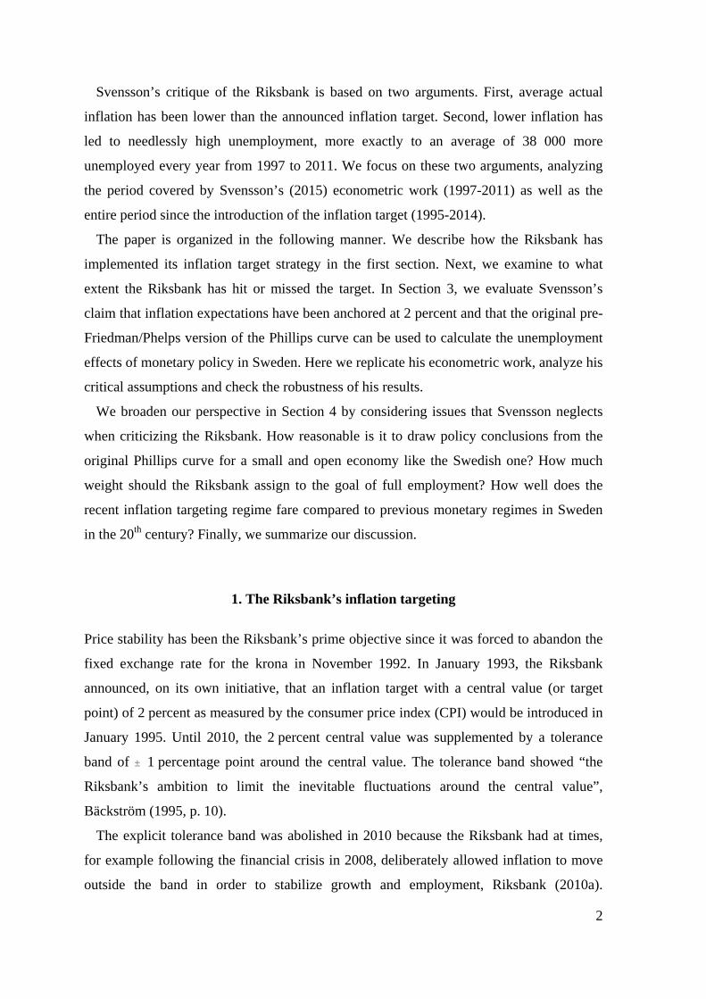
Svensson’s critique of the Riksbank is based on two arguments. First, average actual

inflation has been lower than the announced inflation target. Second, lower inflation has

led to needlessly high unemployment, more exactly to an average of 38 000 more

unemployed every year from 1997 to 2011. We focus on these two arguments, analyzing

the period covered by Svensson’s (2015) econometric work (1997-2011) as well as the

entire period since the introduction of the inflation target (1995-2014).

The paper is organized in the following manner. We describe how the Riksbank has

implemented its inflation target strategy in the first section. Next, we examine to what

extent the Riksbank has hit or missed the target. In Section 3, we evaluate Svensson’s

claim that inflation expectations have been anchored at 2 percent and that the original pre-

Friedman/Phelps version of the Phillips curve can be used to calculate the unemployment

effects of monetary policy in Sweden. Here we replicate his econometric work, analyze his

critical assumptions and check the robustness of his results.

We broaden our perspective in Section 4 by considering issues that Svensson neglects

when criticizing the Riksbank. How reasonable is it to draw policy conclusions from the

original Phillips curve for a small and open economy like the Swedish one? How much

weight should the Riksbank assign to the goal of full employment? How well does the

recent inflation targeting regime fare compared to previous monetary regimes in Sweden

in the 20th century? Finally, we summarize our discussion.

1. The Riksbank’s inflation targeting

Price stability has been the Riksbank’s prime objective since it was forced to abandon the

fixed exchange rate for the krona in November 1992. In January 1993, the Riksbank

announced, on its own initiative, that an inflation target with a central value (or target

point) of 2 percent as measured by the consumer price index (CPI) would be introduced in

January 1995. Until 2010, the 2 percent central value was supplemented by a tolerance

band of ± 1 percentage point around the central value. The tolerance band showed “the

Riksbank’s ambition to limit the inevitable fluctuations around the central value”,

Bäckström (1995, p. 10).

The explicit tolerance band was abolished in 2010 because the Riksbank had at times,

for example following the financial crisis in 2008, deliberately allowed inflation to move

outside the band in order to stabilize growth and employment, Riksbank (2010a).

3

Removing the tolerance band did not change the implementation of the Riksbank’s

monetary policy.

As monetary policy affects inflation with a time lag of a few years, the Riksbank sets its

repo rate such that “inflation is expected to be reasonably close to the target in two years”,

Riksbank (2010b, p. 6). The Riksbank also takes the short-term effects of monetary policy

on growth and employment into account. Thus, the Riksbank can temporarily allow

inflation to deviate from the central value in order to stabilize the overall economy,

Heikensten (1999) and Riksbank (2010b, c and 2013). The average inflation outcome can

for this reason deviate from the central value if the economy is hit by a set of asymmetric

shocks, either negative or positive ones.

In the short run, CPI-inflation is directly affected by changes in the Riksbank’s repo rate

via interest costs on owner-occupied housing. If the repo rate is raised, CPI-inflation

increases. Likewise, if the repo rate is reduced, CPI-inflation decreases. In other words,

when the Riksbank reduces the repo rate with the aim of raising inflation over the medium

term, the short-run inflation effect is the opposite.2 The Riksbank disregards this effect of

a change in the repo rate on CPI-inflation by focusing on the medium- to long-term

inflation horizon, because “to try to counteract a reduction in CPI created by the direct

effects of interest rate cuts with further cuts would, in terms of monetary policy, be

tantamount to chasing one’s own tail”, (Heikensten 1999, p.10). In the long run, when

presumably repo rate increases and decreases have been of the same magnitude, the

average interest rate effect on CPI-inflation will be close zero.

The Riksbank adopts different measures of the underlying rate of inflation to eliminate

the short-run interest rate effect on CPI-inflation. A key measure here is CPIF-inflation

which is calculated assuming a fixed mortgage interest rate. This index is used in the

Riksbank’s DSGE-model of the Swedish economy and in its monetary policy decisions.3 4

Svensson (2013b) stresses that CPIF is an important inflation measure for the Riksbank.

Following the large reductions of the repo rate in 2008 and 2009 and consequently a

decline in CPI-inflation, he noted “there is a generally accepted principle that over the

coming few years it is CPIF-inflation that is relevant. The reason for this is that in the

2

Palmqvist (2013) stresses that the CPI for Sweden is more sensitive to changes in the repo rate than the CPI of other countries. 3

The DSGE-model used by the Riksbank is described in Adolfson et al (2013). 4

CPIF was introduced as a measure of underlying inflation in 2008. See Hansson and others (2008). Other measures of underlying inflation were previously used, but these “removed a little too much” (Riksbank 2010c, p. 60). As these measures removed too much, we have based our examination on CPIF for the entire period. See also Wickman-Parak (2008).

4

short term, CPI-inflation is affected directly by the Riksbank’s own policy-rate

adjustments and monetary policy should not react to these temporary effects”.5, 6

Since 1999, a price stability objective has been inscribed in the Riksbank Act.

According to the preparatory works for the Act, this objective should “be interpreted in

terms of change, not in absolute terms, i.e. the objective should be stated as a target for the

inflation rate rather than as a target for the absolute price level", (Bill 1997/98:40, p. 53).7

Thus, if inflation deviates from the central value, the Riksbank should not compensate for

this deviation. The Riksbank does not respond to undershooting with overshooting or vice

versa. In short, there is no memory built into the inflation target: bygones are bygones. At

each decision point, the repo rate is set to achieve a future inflation rate without any

considerations of the past outcome. Consequently, a comparison between the inflation

outcome and the central value “does not necessarily show how well monetary policy has

been conducted”, Riksbank (2013).

To sum up, the Riksbank’s view of the inflation target, as its official documents make

clear, is as follows: since 1995, the objective has been to hold CPI-inflation as close to the

2 percent central value as possible, within an explicit tolerance band up to 2010, and

within an implicit band thereafter. Minor deviations from the central value do not mean

that the Riksbank has missed or disregarded its inflation target. The Riksbank has

sometimes deliberately allowed CPI-inflation to deviate from the central value to support

growth and high employment. CPIF is thus an alternative and better inflation measure than

CPI when evaluating Swedish monetary policy over the medium-run.

2. Has the Riksbank missed its inflation target?

In this section we analyze the average inflation outcome compared to the inflation target

because this comparison represents a key element in Svensson’s critique of the Riksbank.

Unlike Svensson, who focuses on CPI-inflation, we also examine CPIF-inflation for the

reasons given above. In addition to these two measures of inflation, the perceived rate of

5

The same argument is given by Bergström and Boije (2005). 6

Other central banks exclude mortgage costs as well. The Bank of England and the European Central Bank use price indices where mortgage costs are not included while the Reserve Bank of Australia and the Reserve Bank of New Zealand target underlying inflation where the mortgage costs effect has been eliminated. For an international comparison see for example Pétursson (2004).

7 At the monetary policy meeting of the Riksbank board in February 2009, Lars E O Svensson and Svante Öberg discussed whether

the Riksbank would temporarily gain by switching to a price level stability objective. Öberg thought that such a step would damage the Riksbank’s credibility. No change was made.

5

inflation by households is of vital interest. This measure is obtained through surveys,

where a representative selection of the public answers the question: “compared with 12

months ago, how many percent higher do you think prices are now?” The perceived rate of

inflation is a valuable complement to official price indices as households to a major extent

base their expectations of future inflation on their perceived rates of present inflation.8

Again we emphasize that the average inflation outcome is not necessarily a good measure

of how successful the Riksbank has been in meeting its target since the Riksbank at times

has deliberately allowed inflation to deviate from the central value.

Table 1 shows average inflation and deviations from the central value for three periods,

the entire inflation targeting period 1995-2014, the years examined by Svensson (2015)

1997-2011, and the period preceding the financial crisis 1995-2008. Figure 1 depicts the

inflation rate according to these three series and the tolerance band surrounding the central

value up to 2010.9 The difference between CPI-inflation and CPIF-inflation (i.e. the effect

of changes in the mortgage interest rate) is depicted in Figure 2 together with changes in

the Riksbank’s repo rate.

CPI-inflation, the principal measure studied by Svensson, displays the lowest rate of

inflation, regardless of the choice of period. Average CPI-inflation is between 0.5 and 0.7

percentage points below the central value of 2 percent depending on the period examined.

The main part of this deviation is explained by the downward trend in the repo rate, and

the subsequent decline the mortgage interest rates, since the end of the 1990s, which is

reflected in Figure 2.10 After 1998, there is an almost perfect correlation between the

difference between CPI-inflation and CPIF-inflation and changes in the repo rate. In other

words, changes in the mortgage cost of owner-occupied home follow closely changes in

the Riksbank’s repo rate.

[FIGURES 1 and 2]

CPIF-inflation, which assumes fixed mortgage cost, is between 0.1 and 0.3 percentage

points below the central value. If we disregard the large shocks associated with the global

8

Jonung (1981) argues that perceived inflation is an excellent complement to Statistic Sweden’s official consumer price index. On this point see also Jonung and Laidler (1988).

9 Our data sources are described in Appendix 1.

10 Irma Rosenberg (2007), as a member of the Executive Board of the Riksbank, explained it thus: “between 1995 and 2006,

inflation averaged 1.3 percent measured with CPI. Inflation measured with UND1X, on which we normally base monetary policy, averaged 1.7 percent in the same period. … Regardless of the measure used, the price stability objective as given in the law of the Riksbank has been achieved. On average, however, inflation has been lower than the inflation target defined by the Riksbank”. (In 2008, CPIF replaced UND1X as a measure of the underlying rate of inflation.)

6

financial crisis and the European debt crisis, average CPIF-inflation is 1.9 percent. It

deviates only -0.1 percentage points from the 2 percent central value.

Judging from Figure 1, the Riksbank has been successful in stabilizing average inflation

close to 2 percent. The large reduction in inflation in 2009 following the financial crisis

and the increase in inflation during 2011 is mostly due to changes in the mortgage interest

rate, influenced by the Riksbank’s repo rate. We regard the small difference between

actual inflation and the target as a sign of a successful inflation targeting.

Turning to the perceived rate of inflation, the average is about the same or somewhat

higher than the central value of 2 percent. Thus, households’ perceived inflation has on

average been very close to the central value. Here too the Riksbank deserves a clear pass.

[TABLE 1]

We summarize our results as follows. Based on the Riksbank’s goal of keeping inflation

within a tolerance band of plus/minus one percentage point from the central value of 2

percent, the Riksbank has on average met its inflation target according to our three

measures of inflation from 1995 to 2014. CPIF-inflation is 1.7 percent, only -0.3

percentage points from the target if we, like the Riksbank, exclude the effect on inflation

of changes on the mortgage rate. Svensson’s (2013a) claim that the Riksbank has

“systematically disregarded the inflation target by allowing an average inflation that is

significantly lower than the target of 2 percent” is not supported by the data.

Svensson’s view that the Riksbank must hit 2 percent on average to fulfil its target

implies that the Riksbank should behave as a price level targeter - not as an inflation

targeter. This is a misleading view as the Riksbank’s strategy is based on inflation

targeting where bygone “misses” are bygones. Thus, the Riksbank does not compensate

any over- or undershooting in the past in order to stay at exactly the target value.

In addition, when the deviations from the central value are as small as in Table 1,

potential measurement errors in the data should be considered. According to Statistics

Sweden’s estimates, the margin of error in the annual estimates of CPI-inflation is ± 0.3

percentage points.11 Furthermore, in 2005, Statistics Sweden introduced a change in the

method of calculating indices for inflation that affected the weights in CPI and CPIF. This

affected the estimates of inflation: both CPI- and CPIF-inflation are on average 0.2

11

http://www.scb.se/Statistik/PR/PR0101/_dokument/PR0101_BS_2013.pdf.

7

percentage points lower using the new methodology to construct the price indices

compared to the old methodology.12 This difference in the inflation rate is small, but as our

measures of inflation deviate relatively little from the central value, the impact on the

margin of error from the change in method are not negligible. In our view, to be able to

say with certainty that inflation has deviated from the central value, average inflation

deviations should be considerably larger than in Table 1.13

3. Has the original Phillips curve returned?

Svensson (2015) claims that there is a stable long-run non-vertical Phillips curve for

Sweden – similar to the original Phillips (1958) curve. Using this curve, he concludes that

the policy of the Riksbank has contributed to 38 000 more people being unemployed on

average every year. The original curve, assuming constant inflation expectations over

time, was the prime target in Friedman (1968), where he presented the expectations-

augmented Phillips curve, commonly classified as the neoclassical version of the Phillips

curve. By introducing error-learning or adaptive expectations, Friedman rejected the

assumption of constant expectations leading to the conclusion that the short-run Phillips

curve is unstable and the long-run Phillips curve is vertical.

We examine the robustness of Svensson’s econometric analysis, in particular his crucial

assumption of constant inflation expectations anchored at the central value of 2 percent.

This assumption is central for his assertion that the Riksbank’s policy, by undershooting

the target rate, has contributed to persistently higher unemployment.

We begin by estimating different Phillips curves – Svensson’s version of the original

Phillips curve along with the New Keynesian Phillips curve and the neoclassical Phillips

curve - in Section 3.1. We replicate Svensson’s results, and test his assumption that

inflation expectations have been anchored at 2 percent. Next, in Section 3.2, we bring the

inflation expectations of different groups, households, firms and unions, into the

12

Here our basis is the period 1995Q1 to 2004Q4, i.e. the period for which we have inflation data under both the old and the new method. Inflation data for the period after 2005 Q1 are only available under the new method.

13 Econometric work based on survey data on the perceived and expected rate of inflation uses commonly averages over the

respondents given numerical values. This approach, adopted in Figure 1 and 2, ignores the uncertainty that the respondents assign to

their replies. People associate their perceived and expected rates with considerable uncertainty as demonstrated in Jonung (1986). For

example, where the perceived inflation rate is 2.2 percent as in Table 2, there is an unknown confidence interval surrounding this point

estimate that should be kept in mind when using the survey responses to evaluate the Riksbank’s inflation targeting.

8

econometric analysis. We summarize our results and discuss the policy use of the Phillips

curve in Section 3.3.

3.1 Estimating the Phillips curve

The expectations-augmented Phillips curve is given by::

∗ , (1)

where is inflation, expected inflation, ∗ the unemployment gap, i.e. how

much actual unemployment ( ) deviates from equilibrium unemployment ( ∗ , is a

parameter with a positive value and is a supply shock.14 Svensson (2015) assumes that

both inflation expectations and equilibrium unemployment are constant. Imposing these

two assumptions, Svensson estimates the following econometric model:

(2)

where is the short-run slope of the Phillips curve and represents the long-run slope

of the Phillip’s curve.15 The long-run parameter is the main parameter of interest as

Svensson uses it to calculate the long-run unemployment effect.

Svensson estimates the model using quarterly inflation at an annual rate for the period

1997Q4 to 2011Q4. The inflation target was introduced in 1995Q1, but Svensson argues

that inflation expectations did not become constant until the end of 1997. For this reason,

he excludes the first years of the inflation targeting regime.

In Column 1 in Table 2, we replicate Svensson’s results. The estimated short-run

parameter is -2.68 and the long-run parameter is -0.80, almost identical to Svensson’s

estimates of -2.70 and -0.81. We also estimate the same model for CPIF-inflation for

which the estimated long-run parameter is -0.34 and the estimated short-run parameter -

0.53.16 As discussed previously, the only difference between CPIF and CPI is that the

inflation effect of changes in the mortgage interest rate is excluded from CPIF. Part of the

correlation between unemployment and CPI-inflation is therefore a correlation between

14

See equation (1) in Svensson (2015). 15

As a robustness check, we also estimate Phillips curves using the Riksbank’s estimate of equilibrium unemployment. These estimates are similar to the ones presented above. The assumption of constant equilibrium unemployment has no major effect on the results.

16 CPIF was introduced in 2008, replacing CPIX. There are no major differences between the results for CPIF and CPIX, thus we

only show the results for CPIF.

9

the mortgage rate and unemployment. We can interpret this correlation as a Taylor-rule

effect since the mortgage rate is highly correlated with the repo rate (the correlation

between the repo rate and the 5-year mortgage rate is 0.90). As shown by Figure 3, the

changes in the repo rate, in turn, are highly correlated with changes in unemployment as

predicted by the Taylor-rule. The correlation is especially strong during the sample period

Svensson studies. The correlation is lower before 1997Q4 and after 2011Q4.

These results clearly show that changes in unemployment induced the Riksbank to

change the repo rate, which in turn affected the mortgage rate and through its effect on the

cost of owner occupied homes the rate of CPI-inflation. Thus, it is misleading to claim that

the correlation between CPI-inflation and unemployment is only a Phillips curve effect as

this correlation also captures the Riksbank’s response to changes in the business cycle,

that is in unemployment.

[FIGURE 3]

As there is a clear relationship between unemployment and the Riksbank’s monetary

policy, the estimated adjusted R2 is relatively high for the CPI-inflation model (0.27). For

CPIF-inflation adjusted R2 declines to a mere 0.04. Most of the correlation between CPI-

inflation and unemployment is thus related to the Riksbank’s response to unemployment

rather than to the relationship between consumer prices and unemployment, i.e. the

Phillips curve effect. The very low R2 for CPIF-inflation of 0.04 suggests that the simple

Phillips curve is of little use for drawing policy conclusions.

Svensson argues that inflation expectations were anchored at 2 percent during the period

1997Q4-2011Q4. We test this claim by expanding the sample to include the full inflation

targeting period from 1995Q1 to 2014Q3 (last observation available at the time of data

collection) to carry out two breakpoint tests (Quandt-Andrews and Bai-Perron breakpoint

tests) to examine if there is a significant break in the parameters. According to Svensson,

we should expect one break in 1997Q4 and one in 2011Q4. The first test (Quandt-

Andrews) only allows for one breakpoint while the second test (Bai-Perron) can detect

several breakpoints. Given the limited sample, we restrict the test to detect a maximum of

two breakpoints.17

17

Expanding the data set runs into a problem as the method to calculate the unemployment rate was revised in 2010 by Statistics Sweden. Svensson uses the old unemployment rate in his study. So far we have done the same. But for recent years only the new unemployment rate is available, forcing us to use the new series from now on. However, this does not alter the results as shown in Columns 3 and 4 in Table 2.

10

Estimates for the full inflation targeting period are displayed in Columns 5 and 6 in

Table 2. The two breakpoint tests demonstrate that the Phillips curve is not stable as there

are breaks in the parameters over time. The first breakpoint occurs in 1998Q1, close to the

breakpoint in 1997Q4 selected by Svensson. The second breakpoint takes place in

2008Q4, not in 2011Q4 according to Svensson.

The breakpoint tests suggest the Phillips curve is not stable for the entire period 1997-

2011, indicating that the curve is not useful for calculating the effect of inflation on

unemployment as Svensson does. The breakpoint in 2008Q4 coincides with the break in

the relationship between the repo rate and the unemployment rate displayed in Figure 3.

As argued above, it is likely that the global financial crisis changed the Riksbank’s

response to changes in unemployment.

We also estimate the model for 1998Q1-2008Q4, the period for which our tests indicate

that the model is stable. Applying the breakpoint tests to these new regressions, we find

another break, this time in 2007Q4. Again, this brings us back to our previous conclusion

that the simple original Phillips curve is a faulty guide for policy evaluations as it changes

shape continuously.

[TABLE 2]

The neoclassical and new-Keynesian Phillips curves

Next, we expand the model by including actual inflation expectations – as measured by

two different surveys - to examine Svensson’s claim that his data on inflation expectations

have no significant effect in his regression model and that he can consequently assume

that inflation expectations are constant.

Figure 4 shows inflation expectations with a one-year horizon for four major groups in

Swedish society: households, employer organizations, unions and firms for 1995-2014.

Data on expected inflation of firms is collected by the National Institute of Economic

Research (NIER) and on expected inflation of labor market organizations one year ahead

by TNS Sifo Prospera. These are calculated as the average of inflation expectations held

by employer organizations and by unions. The NIER data is based on a representative

sample of 6,000 firms. The Prospera data includes approximately 50 labor market

organizations (the actual number varies over time). As a large sample size implies data of

11

higher quality than data from a small sample, we expect the NIER data to be a more

reliable estimate of inflation expectations than the Prospera data.

[FIGURE 4]

Figure 4 also depicts the rate of inflation that employer organizations and unions expect

two years and five years ahead.18 Inflation expectations have fluctuated between 0.5 and 4

percent during this period. One-year-ahead expected inflation is more volatile than the

two-year and five-year-ahead expected inflation. Firms often have slightly lower inflation

expectations than the other groups while the opposite holds for households. Data on

inflation expectations in Sweden as shown in Figure 4 clearly demonstrate that expected

inflation has not been constant over time. Svensson’s crucial assumption of constant

inflation expectations is not consistent with actual data for major groups in Swedish

society.19

We estimate two expectations augmented Phillips curves - the New-Keynesian Phillips

curve and the neoclassical Phillips curve - using actual expectations. Following Svensson

for the New Keynesian Phillips curve, we estimate the following model:

| (3)

where | is the expected inflation rate in period t-1 for period (t-1)+4, i.e.

expected inflation one year ahead. To avoid problems with endogeneity, we follow

Svensson’s approach and lag inflation expectations one quarter compared to what the

theoretical model predicts.

For the neoclassical Phillips curve, we estimate the following model:

| , (4)

where | is the expected inflation rate in period t-4 for period t, i.e. expected

inflation one year ago.

A potential econometric problem when including inflation expectations is that Svensson

measures inflation as the quarterly increase in the price index, while inflation expectations

18

Households answer the question “how many percent do you think prices will rise in the next 12 months”. Employer organizations and unions answer the question “how much inflation do you expect in Sweden… measured as the percentage change in the consumer price index”.

19 Svensson (2015) includes data on inflation expectations. However, these are derived from surveys of a small and unrepresentative

group of actors in the private sector. He finds this measure of expectations insignificant in his estimates. Contrary to his result, our estimates of the Phillips curve show that as a rule actual inflation expectations are significant.

12

measures the expected yearly inflation rate (i.e. four quarters ahead). The quarterly

inflation rate and the yearly inflation rates are related but they follow slightly different

processes. Let us calculate the quarterly inflation rate as:

4 (5)

where P is the price index, in this case the CPI, seasonally adjusted. Also, let us calculate

the yearly inflation rate as:

∑ . (6)

As seen from equation (6), the yearly inflation rate is the sum of four quarterly inflation

rates. The yearly inflation rate is smoother than the quarterly inflation rate since some of

the short-term volatility in the quarterly rate cancels out in the summation of the quarterly

rates. More important, the yearly inflation rate is phase-shifted between one or two

quarters compared to the quarterly inflation rate. Quarterly inflation commonly

peaks/bottoms out about one to two quarters ahead of the annual inflation rate.20 In fact, a

Granger causality test shows that the quarterly inflation rate Granger causes the annual

inflation rate. This phase-shift may bias the parameter estimates downwards and make

them less significant.

The phase shift is illustrated in Figure 5a and Figure 5b, depicting quarterly and annual

CPI-inflation and CPIF-inflation, respectively. Here quarterly inflation is more volatile

than annual inflation. The phase shift is also visible. For example, during the financial

crisis in 2008/09, CPI-inflation fell sharply. Quarterly CPI-inflation bottomed out in

2009Q1 while annual inflation bottomed out first in 2009Q3.

[FIGURE 5]

There is no simple method to solve the phase-shift problem. Svensson chooses to ignore

it by mixing quarterly inflation with annual inflation expectations. Svensson’s

combination of yearly and quarterly data on inflation causes a well-known problem with

overlapping data. Overlapping data usually makes the errors in the model auto-correlated.

An endogeneity problem may also emerge, biasing the parameter estimates. The only way

to avoid overlapping data when using yearly inflation is to use yearly data observations for

20

A similar example concerning GDP growth is given by Bank of Canada. See http://www.bankofcanada.ca/core-functions/monetary-policy/framework/measuring-economic-growth.

13

all variables involved. In our case, this approach is not feasible as we have too few data

points.

Given that there is no simple solution to this econometric problem, we adopt two

approaches. First, we estimate, similar to Svensson, the model mixing quarterly inflation

with yearly inflation expectations. Second, we also estimate the model with yearly

inflation and inflation expectations from quarterly data and use instrumental variables to

address any potential endogeneity problem.21 Our main conclusions hold irrespective of

which method we adopt: inflation expectations are significant in the Phillips curve –

contrary to Svensson’s claim of the opposite.

Estimates of the New Keynesian Phillips curve for CPI-inflation 1997Q4-2011Q4 are

shown in Columns 1 and 2 in Table 3. Firms’ inflation expectations are significant in the

model at the 1 percent significance level, while the unemployment rate has no significant

effect once firms’ inflation expectations are included. Prospera’s inflation expectations are

not significant in the model, which is potentially caused by the phase-shift in the data. A

Granger causality test reveals that firms’ inflation expectations Granger cause inflation

expectations of labor market organizations by approximately one quarter, suggesting that

firms may be better informed than labor market organizations. From a technical point of

view this result also lends some support to the view that the phase-shift problem has a

larger impact on the model when we use the inflation expectations from labor market

organizations compared to those of firms. For the neoclassical model, inflation

expectations have no significant effect, irrespective of which measure of inflation

expectations adopted.

Expanding the sample to the full inflation targeting period, we find that the inflation

expectations of firms are significant both in the New Keynesian and the neoclassical

models. Expectations of employer organizations and unions are only significant at the 10

percent level in the New Keynesian model. Similar to the original Phillips curve we find

two breakpoints – one in 1998Q1 and one in 2008Q4.

These two breakpoints emerge - not by the effect of inflation expectations changing as

Svensson argues - but because the relationship between the unemployment rate and the

repo rate (i.e. Riksbank’s reaction function) changed after the Great Recession. Turning to

CPIF-inflation (see Table 4), we find no breakpoints once inflation expectations are

included in the model. Moreover, looking at the full inflation targeting period for which

21

These results are available upon request from the authors.

14

we have the most data and thus the most accurate parameter estimates, we find inflation

expectations to be significant. For the firms, inflation expectations are significant both in

the New Keynesian model and the neoclassical model at the 5 percent significance level.

Inflation expectations of labor market organizations are significant at the 10 percent level

for the neoclassical model. The unemployment rate is in 6 out 8 cases not significant in the

models once inflation expectations are included.

These results for CPIF-inflation lend support to our previous conclusion that we cannot

rule out the case that inflation expectations are time varying. But, and perhaps most

importantly, the explanatory power of all models is low, irrespective of how we model

CPI- and CPIF-inflation. The simple Phillips curve model, with or without data on

inflation expectations, is obviously not suitable for drawing policy conclusions.

[TABLE 3 and 4]

3.2 Inflation expectations and expectation errors

According to Svensson’s analysis the expectations gap, i.e. the difference between

inflation and expected inflation should be negative and the unemployment gap should be

positive. In this section we analyze if his view is supported by the data.

We reconfigure the Phillips curve model in equation (1) so that the “expectations gap”

or the expectations error, i.e. the deviation between actual inflation and expected inflation,

is on the left hand side and the unemployment gap on the right hand side:

∗ . (10)

In the Neoclassical model, the expectations gap is the difference between current

inflation and expected inflation in the preceding period, in our case four quarters before

( | ). In the New Keynesian model, the expectations gap is given as the difference

between current inflation and expected future inflation ( | ).

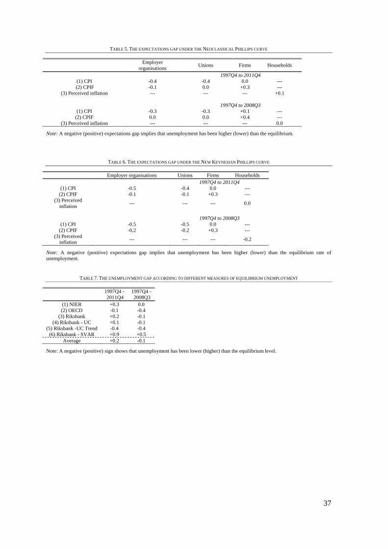
The expectations gap for the Neoclassical Phillips curve is shown in Table 5 and for the

New Keynesian Phillips curve in Table 6. The expectations gap is estimated for two

periods: 1997-2011, the period Svensson (2015) studies, and 1997-2008, the period before

15

the financial crisis.22 A minus sign means that actual inflation is lower than expected

inflation and a plus sign indicates that actual inflation is higher than expected inflation.

[TABLES 5 and 6]

The expectations gap measured by CPI-inflation is negative when we look at the

inflation expectations of employer organizations and unions, regardless of the model and

time period selected. The expectations gap is negative because these groups have

misjudged the future repo rate and its impact on the cost of housing.23 With respect to

CPIF-inflation, the expectations gap is between -0.3 and 0.0 for the two groups, depending

on the time period.

Based on the inflation expectations of firms, the expectations gap is 0.0 for CPI-inflation

and +0.3 for CPIF-inflation. This result indicates that average unemployment has been

below equilibrium unemployment on average. Households’ expectations gap is between

0.0 and +0.1, i.e. both positive and negative, but very close to zero.

Available data on inflation expectations do not provide any clear answer to the question

of whether the expectations error is negative, zero or positive.24 However, the gap is small

in all cases as displayed in Table 5 and 6. Svensson’s conclusions about the expectations

error and the employment gap are thus not robust.

One of Svensson’s key arguments is that the negative expectations error, assuming

constant inflation expectations, has caused wages to increase “too” rapidly. This claim is

not supported by data on real unit labor cost. The average yearly change in the real unit

labor cost is negative, -0.3 percent for the full period (1997Q4-2011Q4) and -0.2 percent

for the period before the financial crisis (1997Q4-2008Q3). The average change in the real

unit labor cost supports our conclusion that inflation expectations have adjusted to changes

in inflation and that real wages have not increased “too” fast.

Instead of examining the expectations gap or expectations error on the left hand side of

equation (10), we can analyze the unemployment gap, i.e. the difference between actual

unemployment and equilibrium unemployment, the right hand side of equation (10). If the

22

As the questions about inflation expectations are constructed in different ways, we compare inflation expectations held by employer organizations, unions and firms with CPI- and CPIF-inflation and expected inflation of households with their perceived inflation.

23 This is evident from the correlation of 0.9 between the forecast errors for these two groups for CPI-inflation and for the repo rate.

24 Flodén (2012) finds that the expectations held by firms are the most reliable measure for explaining nominal wage growth. Which

inflation expectations – for example those of the business sector or those of the public – that are the most relevant to use in empirical work depends on the issue to be addressed.

16

gap is negative, unemployment has been lower than the equilibrium unemployment. If the

gap is positive, unemployment has been higher. As the expectations gap of the Phillips

curve in Tables 5 and 6 is small, we expect that the unemployment gap to be small as well.

All estimates of equilibrium unemployment are notoriously uncertain. According to the

Riksbank, it lies within the interval 5-7.5 percent. As the estimates are imprecise, we use

six different measures of equilibrium unemployment in our calculations: the NIER and the

OECD measure and four estimates by the Riksbank; see Table 7. Svensson (2015) uses

measure number (3) in Table 7.

[TABLE 7]

The average unemployment gap lies within the interval of -0.4 and +0.9 percentage

points, depending on the measure of equilibrium unemployment we use and the period

analyzed. If we consider the first three unemployment gaps in Table 7 – that of NIER and

of OECD and the estimate from the Riksbank that Svensson has chosen – the

unemployment gap is between -0.1 and +0.3 for the entire period 1997-2011. For the

period preceding the financial crisis, the average gap is between -0.4 and 0.0. Here

registered unemployment has been lower than equilibrium unemployment according to

these measures. When we take an average of all these unemployment gaps, the gap is +0.2

for 1997-2011 and -0.1 for the period preceding the financial crisis.

Taken together, these figures demonstrate that the deviations from equilibrium

unemployment are small. They usually lie within the interval of -0.2 and +0.2. Thus, there

is no support for Svensson’s claim that the unemployment gap has been as large as +0.8

percentage points.

Svensson (2012, 2015) maintains that the Riksbank has overestimated equilibrium

unemployment by 0.75 percentage points. The source for his argument is that the average

expectations gap is negative if inflation expectations are assumed to be constant over time

at 2 percent. However, as the average unemployment gap is near zero, Svensson is pushed

to the conclusion that the Riksbank has overestimated equilibrium unemployment. This is

necessary to enable his model and his assumption of constant inflation expectations to be

combined within a consistent framework. Thus, in practice Svensson is forced to reject not

only the Riksbank’s estimates of equilibrium unemployment, but also those of the OECD

and the NIER, which largely coincide with the measures of the Riksbank.

17

We do not find any support in our estimates that the Riksbank has overestimated

equilibrium unemployment when we use actual data on inflation expectations. Instead, our

results show that both the average expectations gap and the average unemployment gap

have been near zero. From these numbers, we conclude that Svensson (2012, 2015) relies

too heavily on his assumption of constant inflation expectations in his critique of the

Riksbank.

3.3. How useful is the Phillips curve for monetary policy evaluation?

Our main conclusion that it is not possible to claim that the Riksbank has contributed to

making 38 000 people unemployed on average every year is supported by Söderström and

Vredin (2013). Using the Riksbank’s DSGE-model, the Ramses model, they reach the

following conclusion on the issue of whether monetary policy has contributed to any long-

term employment effects: “the honest answer is that we simply do not know, not even

when we use the best scientific methods available and even if we accept one of these

calculations, it does not necessarily mean that monetary policy could have been conducted

in a better way when the decisions were actually made”.

The European Central Bank (2014), in a survey of the use of Phillips curves in monetary

policy analysis and decision-making, finds that uncertainty relating to both model

specification and the measure of slack in the economy reduces the reliability and thus the

usefulness of the Phillips curve. Similarly, Jürgen Stark from the ECB stresses that

reduced form models such as the Phillips curve short-circuit the workings of a complex

economy (Fuhrer et al, 2009). Stock and Watson (2010) make a similar remark concerning

the US record; “the history of the inflation forecasting literature is one of apparently stable

relationships falling apart upon publication.” Our estimates of various versions of the

Phillips curve for Sweden during recent decades are in line with these remarks pertaining

to the euro area and the United States.

Another warning against using a Phillips curve approach for evaluating monetary policy

stems from Goodhart’s law.25 According to this “law”, any statistical correlation between

a few economic variables will disappear once policy-makers try to exploit the correlation

for policy purposes. In other words, any perceived stable correlation between

unemployment and inflation is likely to evaporate if the Riksbank tries to reduce

25

Goodhart’s law is basically a version of the Lucas critique applied to monetary policy, see, for example Chrystal and Mizen (2003).

18

unemployment by increasing inflation – even if there was ex ante evidence of a stable

long-run non-vertical Phillips curve.

4. The inflation target in a broader perspective

4.1. Monetary policy and unemployment in a globalized world

How much economic policy autonomy does Sweden have in influencing the domestic

business cycle and thus domestic unemployment? To what extent can monetary policy

mitigate external shocks such as that one in 2009, when Sweden’s exports of goods fell by

18 percent? Could this loss in exports be rapidly replaced by higher domestic consumption

and investment using a lower interest rate? A substantial part of the decline in growth

since the financial crisis erupted can be attributed to slower export growth. Between 2010

and 2014, real private consumption grew by an average of 2.2 percent a year, close to the

average growth rate of 2.8 percent between 1995 and 2007. Real export growth, however,

declined from an average of 7.2 percent a year between 1995 and 2007 to an average of

4.4 percent a year between 2010 and 2014.26

To illustrate the Swedish business cycle’s international dependence, we estimate a

simple model where Swedish unemployment is set as a function of unemployment in the

United States and the euro area. As a comparison, we estimate the same model for

Australia and Canada. As Sweden, Australia and Canada are small economies compared to

the United States and the euro area, it is reasonable to assume that these countries do not

influence the business cycle in the United States or the euro area. The model we estimate

is the following one:

∑ ∑ , (11)

where u is the change in the unemployment ratio, i stands for Sweden, Australia or

Canada, and t is the time period. We estimate the model for the period 1997 Q4-2013 Q4.

The results are summarized in Table 8.

According to Table 8, external shocks explain between 59 and 61 percent of the

variation in the unemployment rate. For Australia, the share of the variation explained by

the United States and the euro area is lower, probably because Australian exports are more

dependent on the Chinese economy. The high international dependence for the Swedish

26

Data collected from www.scb.se

19

and Canadian economies demonstrates how difficult it is for a small open economy to

avoid a sharp international downturn. There is room for an expansionary monetary policy,

but its impact will be limited.

What does this tell us about Svensson’s criticism of the Riksbank? Svensson does not

take Sweden’s position as a small, open economy, heavily dependent on external

economic influences affecting exports, imports and the financial markets, sufficiently into

account. Implicitly, he uses a model for a closed economy. When evaluating the inflation

target policy of the Riksbank, external shocks and developments should be explicitly

incorporated in the analysis.

[TABLE 8]

4.2. How many objectives should the Riksbank have?

The global financial crisis has revealed a fundamental conflict between financial

stability and inflation targeting. This conflict arises when the central bank stabilizes

inflation based on a consumer price index and simultaneously allows a rapid rise in asset

prices. Developments in the United States before, during and after the financial crisis can

serve as an example of this trade-off, see e.g. Borio (2012) and Leijonhufvud (2007).

Financial stability is a necessary precondition for inflation stability (or monetary

stability). With respect to Sweden, we are of the opinion that the Riksbank must have

financial stability as its primary objective in order to pursue its inflation target. The first

objective is a precondition for the second one. This insight is evident from the Riksbank

Act describing the Riksbank’s tasks. The Riksbank is given the task of promoting a safe

and efficient payments system while maintaining price stability.

Each financial crisis in the past has forced the Riksbank and the Government to

intervene and support the financial system as lenders of last resort. The Riksbank has a

monopoly on producing central bank money, which is the key to the resolution of financial

crises. The history of financial crises in Sweden indicates that the Riksbank should have

financial stability as a most important objective, even though other institutions may also

be assigned the task of promoting financial stability.

When Svensson focuses on unemployment in his criticism of the Riksbank, he shifts the

focus from inflation to employment as a goal for the Riksbank. Indirectly, he introduces a

third objective for the Riksbank, namely high employment. Even though employment is

20

intended to be a secondary monetary policy objective, subject to the primary objective of

price stability within the framework of a flexible inflation target policy, there is a

substantial risk that employment will once again emerge as a key monetary policy

objective. There would thus be three objectives – a difficult situation to manage with clear

risks of conflicts and inconsistencies between the objectives.

Swedish economic policy history provides an important insight about the choice of goals

for monetary policy. When the primary objective of Swedish stabilization policy was full

employment, the social partners were able to achieve high nominal wage increases,

knowing that the Government and the Riksbank would create the inflation required to

make full employment possible. The accommodation policy of the 1970s and 1980s

illustrates the vicious circle of price and wage increases that emerged when the Riksbank

had to pursue such a policy of full employment.

A key lesson from the experience of accommodation and from financial crises is that the

Riksbank should focus on nominal factors such as inflation, the money supply and the

volume of credit, not on real factors such as growth and unemployment. The divorce

between monetary policy and employment policy occurred when inflation was made the

primary economic policy goal around 1990. One reason for making the Riksbank

independent was that it could be given a clearly defined goal – and be made responsible

for it. The Riksbank’s independence would be threatened in the long run if it were to be

involved again in unemployment policy.27

4.3. What does the long-run perspective say about the inflation target?

Svensson takes a short-run view as he examines the policy of the Riksbank only after

1995. It is valuable to supplement this perspective with a longer one. In other words, we

should compare the outcome of the regime of inflation targeting with the performance of

other monetary policy regimes.

There is a unique data source that can be exploited for this purpose, namely data on

Swedish collective agreements that cover the whole economy. According to Fregert and

Jonung (2008), the characteristics of the central collective agreements make it possible to

compare different monetary regimes. They demonstrate that the length and content of the

collective agreements reflect the employers’ and the employees’ expectations about future

27

According to Orphanides (2013), monetary policy in many countries is currently under threat by being burdened with too many objectives.

21

macroeconomic developments. When the social partners expect high and volatile inflation,

the length of wage agreements will be short and vice versa. The length of the wage

agreements is thus an indicator of the state of inflation expectations.

The pattern for the period 1908-2008, as studied by Fregert and Jonung, shows two

periods with long-lasting collective agreements: the gold standard before World War I and

the inflation target policy after 1995. The other stabilization policy regimes are associated

with greater macroeconomic uncertainty. The inflation target policy after 1995 is the only

period in modern times with a long stretch of consistent three-year agreements.

We would like to emphasize that the three-year agreements have survived the global

financial crisis that hit the Swedish economy in 2008-10. The social partners concluded a

special agreement, the so-called crisis agreement, to handle this shock in the short run. But

the long-run agreement remained in force, i.e. the partners did not blame domestic

monetary and fiscal policy for the crisis.

Table 9 displays CPI-inflation and GDP per capita growth during five different

monetary policy regimes – the gold standard 1873-1913, the interwar years 1920-38,

Bretton Woods 1951-73, the accommodation regime 1974-92 and the inflation targeting of

1995-2013. Based on Table 9, the inflation and growth outcomes during the inflation

targeting policy have been relatively favorable, combining high growth with low inflation,

particularly when compared to the accommodation policy of the 1970s and the 1980s.

[TABLE 9]

Furthermore, Sweden’s macroeconomic performance under the recent inflation targeting

regime has been strong. GDP has increased in real terms by 55 percent between 1995 and

2013, comparable with growth in the United States and the United Kingdom, and higher

than growth in Germany or the euro area as a whole. Real wages have grown on average

by 1.9 percent a year. Exports as a share of GDP have grown from 36 percent in 1994 to

peak at 53 percent in 2008. These numbers compare favorably to those of other countries.

During the period of inflation targeting, Sweden has carried out a substantial fiscal

consolidation and introduced a fiscal framework. The inflation targeting regime has been

supported by the fiscal regime and vice versa.28 On the negative side, however, there has

been a prolonged increase in real house prices – 144 percent between 1995 and 2012. This

28

On the role of the fiscal regime, see Jonung (2015).

22

rise is unprecedented in recent times and a possible sign of threatening financial

imbalances. To sum up, the Riksbank’s inflation targeting stands out as successful – at

least so far.

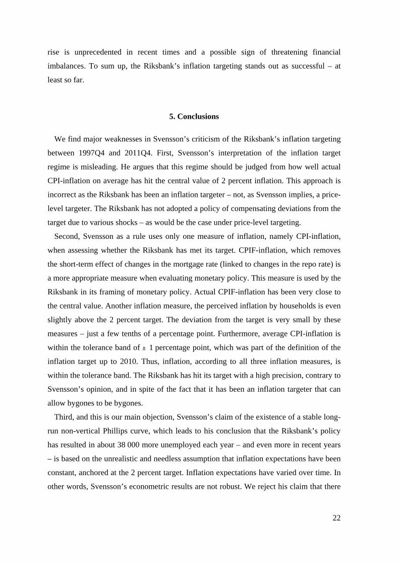
5. Conclusions

We find major weaknesses in Svensson’s criticism of the Riksbank’s inflation targeting

between 1997Q4 and 2011Q4. First, Svensson’s interpretation of the inflation target

regime is misleading. He argues that this regime should be judged from how well actual

CPI-inflation on average has hit the central value of 2 percent inflation. This approach is

incorrect as the Riksbank has been an inflation targeter – not, as Svensson implies, a price-

level targeter. The Riksbank has not adopted a policy of compensating deviations from the

target due to various shocks – as would be the case under price-level targeting.

Second, Svensson as a rule uses only one measure of inflation, namely CPI-inflation,

when assessing whether the Riksbank has met its target. CPIF-inflation, which removes

the short-term effect of changes in the mortgage rate (linked to changes in the repo rate) is

a more appropriate measure when evaluating monetary policy. This measure is used by the

Riksbank in its framing of monetary policy. Actual CPIF-inflation has been very close to

the central value. Another inflation measure, the perceived inflation by households is even

slightly above the 2 percent target. The deviation from the target is very small by these

measures – just a few tenths of a percentage point. Furthermore, average CPI-inflation is

within the tolerance band of ± 1 percentage point, which was part of the definition of the

inflation target up to 2010. Thus, inflation, according to all three inflation measures, is

within the tolerance band. The Riksbank has hit its target with a high precision, contrary to

Svensson’s opinion, and in spite of the fact that it has been an inflation targeter that can

allow bygones to be bygones.

Third, and this is our main objection, Svensson’s claim of the existence of a stable long-

run non-vertical Phillips curve, which leads to his conclusion that the Riksbank’s policy

has resulted in about 38 000 more unemployed each year – and even more in recent years

– is based on the unrealistic and needless assumption that inflation expectations have been

constant, anchored at the 2 percent target. Inflation expectations have varied over time. In

other words, Svensson’s econometric results are not robust. We reject his claim that there

23

is a stable long-run non-vertical Phillips curve for Sweden. The Friedman/Phelps version

of the Phillips curve stands out as superior to the original specification used by Svensson.

In addition to these objections, we bring out three perspectives not considered by

Svensson. First, the Phillips curve is too simple a model for assessing the effects of

monetary policy on unemployment in a small open economy like Sweden. A more

sophisticated model is needed that at least includes external economic influences. In a

deep global crisis, like the Great Recession, unemployment in Sweden is primarily

determined by international developments. The Riksbank has not much scope to influence

Swedish unemployment via monetary policy.

Second, under the Swedish Riksbank Act, the Riksbank has two objectives: financial

stability and price stability. Monetary policy would be overburdened by adding full

employment to the list of monetary policy goals which is the case when the Riksbank is

blamed for employment losses.

Third, Svensson has a short-run perspective as he is looking at the years 1997-2011.

When we compare the Riksbank’s recent inflation targeting regime with monetary policy

regimes over the past 100 years, the Riksbank has clearly been successful in the past

fifteen years. Sweden has not had such stable and low inflation combined with high

economic growth since the pre-World War I gold standard.

All in all, Svensson should be praised for initiating an important debate about Swedish

monetary policy. However, a careful examination shows that his conclusions do not hold.

Most importantly, his claim of establishing a stable long-run non-vertical Phillips curve

that can be exploited for monetary policy purpose is not supported by the data.

Although we find Lars E O Svensson’s critique of the Riksbank misleading, our views

should not be interpreted as an endorsement of the Riksbank's policy. There are reasons to

criticize the conduct of Swedish monetary policy but they should not be based on

Svensson’s approach.

24

REFERENCES

Adolfson, Malin, Stefan Laseen, Lawrence Christiano, Mathias Trabandt and Karl Walentin.

2013. "Ramses II - Model Description". Swedish Riksbank Occasional Paper Series, 12.

Andersson, Björn, Stefan Palmqvist, and Pär Österholm. 2012. The Riksbank’s attainment of

its inflation target over a longer period of time”. Swedish Riksbank Economic

Commentaries, 4.

Bergström, Villy, and Robert Boije. 2005. “Monetary policy and unemployment”. Swedish

Riksbank Economic Review 2005 4, 15-48.

Borio, Claudio. 2012. “The financial cycle and macroeconomics: what have we learnt?”, BIS

working paper, 395.

Bäckström, Urban. 1995, “Price stability and monetary policy”, Riksbank Quarterly Review

1, 5-11.

Chrystal, K. Alec, and Paul D. Mizen. 2003. “Goodhart’s law: its origins, meaning and

implications for monetary policy”, In Paul Mizen, ed., Central banking, monetary theory

and practice. Essays in honour of Charles Goodhart, volume 1, Edward Elgar,

Cheltenham.

European Central Bank. 2014. “The Phillips curve relationship in the euro area”, European

Central Bank Monthly Bulletin, July, pp. 99-114.

Flodén, Martin. 2012. “A note on Swedish inflation and inflation expectations”,

http://people.su.se/~mflod/files/swedishinflation.pdf.

Fregert, Klas and Lars Jonung. 2008. “Inflation targeting is a success, so far: 100 years of

evidence from Swedish wage contracts”, Economics: The Open-Access, Open-Assessment

E-Journal 2, 2008-31.

25

Friedman, Milton. 1968. “The role of monetary policy”. The American Economic Review 58

(1), 1-17.

Fuhrer Jeff, Yolanda K. Kodrzuncki, Jane Sneddon Little and Giovanni P. Olivei. 2009.

“Understanding inflation and implications for monetary policy: A Phillips curve

retrospective”. Cambridge: MIT Press.

Hansson, Jesper, Jesper Johansson and Stefan Palmqvist. 2008. “Why do we need measures

of underlying inflation?”, Swedish Riksbank Economic Review 2, 23-41.

Heikensten, Lars. 1999. “The Riksbank’s inflation target – clarification and evalutation”,

Swedish Riksbank Quarterly Review 1, 5-17.

Jonung, Lars. 1981, “Perceived and expected rates of inflation in Sweden”, American

Economic Review 5, 961-68.

Jonung, Lars. 1986. “Uncertainty of inflationary perceptions and expectations” Journal of

Economic Psychology 4, 315-25.

Jonung, Lars. 2015. “Reforming the fiscal framework: The case of Sweden 1973-2013”, In

Torben. Andersen, Michael. Bergman and Svend Hougard Jensen, eds. Reform Capacity

and Macroeconomic Performance in the Nordic Countries, Oxford University Press.

Jonung, Lars and David Laidler. 1988. Are perceptions of inflation rational? Some evidence

for Sweden”, American Economic Review 78(5), 1080-87.

Jonung, Lars and Erik Wadensjö. 1980. “The Swedish Phillips curve”, Skandinaviska

Enskilda Banken Quarterly Review, 1-2.

Leijonhufvud, Axel. 2007. “The perils of inflation targeting”, June.

http://www.voxeu.org/article/perils-inflation-targeting.

Orphanides, Athanasios. 2013. “Is monetary policy overburdened?”, BIS working papers,

26

435.

Palmqvist, Stefan. (2013). “Konsumentprisindex i Sverige och Kanada är inte så lika”,

Blogg 20/11 2013. Retrieved 16/2-2014.

http://ekonomistas.se/2013/11/20/konsumentprisindex-i-sverige-och-kanada-ar-inte-sa-lika/

Pétursson Thorarinn G. 2004. “Formulation of inflation targeting around the world”.

Sedlabanki Island Monetary Bulleting 2004 (1), 57-84.

Phillips, Alban W. 1958, “The relationship between unemployment and the rate of change of

money wage rates, in the United Kingdom, 1861-1957. “ Economica 25, 283-299.

Regeringens proposition (1997/98:40), Riksbankens ställning.

Riksbanken (2010a), “Monetary policy in Sweden”. Press release 3 June 2010.

http://www.riksbank.se/Upload/Dokument_riksbank/Kat_publicerat/Pressmeddelanden/2010

/nr27e.pdf

Riksbanken (2010b), Monetary policy in Sweden, Stockholm.

Riksbanken (2010c), Monetary policy report, July 2010, Stockholm.

Riksbanken (2013), Account of monetary policy 2012, Stockholm.

Rosenberg, Irma. (2007), “Monetary policy and the labor market”. Speech, Simra

Stockholm, 22/5-2007.

http://www.riksbank.se/en/Press-and-published/Speeches/2007/Rosenberg-Monetary-

policy-and-the-labor-market/

Schön Lennart and Olle Krantz. 2012. “Swedish historical national accounts 1560-2010”.

Lund Papers in Economic History, 123. Lund University.

Stock. James and Mark Watson. 2010. “Modeling inflation after the crisis”, NBER working

27

paper 16488.

Svensson, Lars E. O. 2012. “Correcting the Riksbank's estimate of the long-run sustainable

rate of unemployment,” Appendix 2 of Riksbank July 2012 Minutes.

Svensson, Lars E. O. 2013a. “Sammantagna reala konsekvenser av Riksbankens

penningpolitik”, Blogg Ekonomistas 11/4-2013. Retrieved 02/16-2014.

http://ekonomistas.se/2013/11/04/sammantagna-reala-konsekvenser-av-riksbankens-

penningpolitik/

Svensson, Lars E. O. 2013b. “Reservation against the account of monetary policy 2012”.

Appendix B to the minutes of the Executive Board meeting no. 7, 19 March 2013.

Svensson, Lars E. O. 2015. “The possible unemployment cost of average inflation below a

credible target”, American Economic Journal: Macroeconomics, 7(1): 258-96.

Söderström Ulf and Anders Vredin. 2013. “Inflation, unemployment and monetary policy”.

Riksbank Economic Commentaries, no 1.

Wickman-Parak, Barbro. 2008. “The Riksbank’s inflation target”, speech at Swedbank,

Stockholm 06/09-2008.

28

II. Figures

FIGURE 1. ANNUAL CPI- AND CPI-INFLATION AND PERCEIVED INFLATION 1995Q1-2014Q3

‐2

‐1

0

1

2

3

4

5

6

71995Q1

1995Q4

1996Q3

1997Q2

1998Q1

1998Q4

1999Q3

2000Q2

2001Q1

2001Q4

2002Q3

2003Q2

2004Q1

2004Q4

2005Q3

2006Q2

2007Q1

2007Q4

2008Q3

2009Q2

2010Q1

2010Q4

2011Q3

2012Q2

2013Q1

2013Q4

2014Q3

Per

cen

t

(1) CPI (2) CPIF (3) Perceived inflation Tolerance interval, 1995‐2009

29

FIGURE 2. THE DIFFERENCE BETWEEN ANNUAL CPI- AND CPIF-INFLATION AND THE CHANGE IN THE RIKSBANK’S REPO-RATE, 1995Q1 TO

2014Q3.

‐6.0

‐5.0

‐4.0

‐3.0

‐2.0

‐1.0

0.0

1.0

2.0

3.0

1995Q1

1995Q4

1996Q3

1997Q2

1998Q1

1998Q4

1999Q3

2000Q2

2001Q1

2001Q4

2002Q3

2003Q2

2004Q1

2004Q4

2005Q3

2006Q2

2007Q1

2007Q4

2008Q3

2009Q2

2010Q1

2010Q4

2011Q3

2012Q2

2013Q1

2013Q4

2014Q3

Difference between CPI and CPIF Change in repo‐rate

30

FIGURE 3. THE RATE OF UNEMPLOYMENT AND THE RIKSBANK’S REPO-RATE, 1995Q1 TO 2014Q1

‐4

‐2

0

2

4

6

8

10

0

2

4

6

8

10

12

14

1995Q1

1995Q4

1996Q3

1997Q2

1998Q1

1998Q4

1999Q3

2000Q2

2001Q1

2001Q4

2002Q3

2003Q2

2004Q1

2004Q4

2005Q3

2006Q2

2007Q1

2007Q4

2008Q3

2009Q2

2010Q1

2010Q4

2011Q3

2012Q2

2013Q1

2013Q4

2014Q3

Unemployment rate (left axis) Repo‐rate (right axis)

31

FIGURE 4. EXPECTED INFLATION RATES OF HOUSEHOLDS AND FIRMS, 12-MONTH AHEAD, AND EXPECTED RATES OF EMPLOYER

ORGANIZATIONS AND UNIONS, 12-MONTH, 2-YEAR AND 5-YEAR AHEAD.

Note: No data are available for employer organizations and union expectations for three quarters: 1995Q1, 1995Q4 and 2001Q3.

0.0

0.5

1.0

1.5

2.0

2.5

3.0

3.5

4.0

4.5

1995Q1

1995Q3

1996Q1

1996Q3

1997Q1

1997Q3

1998Q1

1998Q3

1999Q1

1999Q3

2000Q1

2000Q3

2001Q1

2001Q3

2002Q1

2002Q3

2003Q1

2003Q3

2004Q1

2004Q3

2005Q1

2005Q3

2006Q1

2006Q3

2007Q1

2007Q3

2008Q1

2008Q3

2009Q1

2009Q3

2010Q1

2010Q3

2011Q1

2011Q3

2012Q1

2012Q3

2013Q1

Per

cen

t

Employer organisations, 1 year Employer organisations, 2 years Employer organisations, 5 years

Labour organisations, 1 year Labour organisations, 2 years Labour organisations, 5 years

Households, 1 year Firms, 1 year

32

FIGURE 5A. QUARTERLY AND

ANNUAL CPI-INFLATION, 1995-2011.

FIGURE 5B. QUARTERLY AND ANNUAL CPIF-INFLATION, 1995 – 2011.

‐5

‐3

‐1

1

3

5

7

1995Q1

1995Q4

1996Q3

1997Q2

1998Q1

1998Q4

1999Q3

2000Q2

2001Q1

2001Q4

2002Q3

2003Q2

2004Q1

2004Q4

2005Q3

2006Q2

2007Q1

2007Q4

2008Q3

2009Q2

2010Q1

2010Q4

2011Q3

Per

cen

t

CPI inflation, annual CPI inflation, quarterly

‐5

‐3

‐1

1

3

5

7

1995Q1

1995Q4

1996Q3

1997Q2

1998Q1

1998Q4

1999Q3

2000Q2

2001Q1

2001Q4

2002Q3

2003Q2

2004Q1

2004Q4

2005Q3

2006Q2

2007Q1

2007Q4

2008Q3

2009Q2

2010Q1

2010Q4

2011Q3

Per

cen

t

CPIF inflation, annual CPIF inflation, quarterly

33

III. TABLES

TABLE 1. AVERAGE CPI-; CPIF- AND PERCEIVED INFLATION AND DEVIATION FROM THE CENTRAL VALUE

1995Q1 – 2014Q3 1995Q1 – 2008Q3 1997Q4 – 2011Q4 Average inflation

(1) CPI 1.3 1.5 1.5 (2) CPIF 1.7 1.9 1.8

(3) Perceived inflation 2.2 2.0 2.3 Deviation from the central value

(1) CPI -0.7 -0.5 -0.5 (2) CPIF -0.3 -0.1 -0.2

(3) Perceived inflation +0.2 ± 0 +0.3

Source: Andersson, Palmqvist and Österholm (2012) and National Institute of Economic Research.

34

TABLE 2. ESTIMATES OF ORIGINAL PHILLIPS CURVE WITH CONSTANT INFLATION EXPECTATIONS

Price index CPI CPIF CPI CPIF CPI CPIF CPI CPIF Inflation expectations Constant Constant Constant Constant Constant Constant Constant Constant Unemployment rate Old Old New New New New New New

Time period 97Q4-11Q4

97Q4-11Q4

97Q4-11Q4

97Q4-11Q4

95Q1-14Q3

95Q1-14Q3

98Q1-08Q4

98Q1-08Q4

(1) (2) (3) (4) (5) (6) (7) (8)

7.14*** (1.25)

4.14*** (1.14)

6.77*** (1.31)

4.10*** (1.12)

3.73*** (1.24)

2.27** (1.01)

8.96*** (1.16)

5.76*** (1.08)

-0.80***

(0.17) -0.34** (0.15)

-0.74*** (0.18)

-0.33** (0.15)

-0.32** (0.16)

-0.08 (0.12)

-1.08*** (0.16)

-0.58*** (0.15)

-2.68***

(0.82) -0.53 (0.49)

-2.51*** (0.85)

-0.38 (0.51)

-1.95*** (0.77)

-0.34 (0.37)

-1.99** (0.74)

-0.85 (0.73)

--- --- --- --- --- --- --- ---

| --- --- --- --- --- --- --- ---

| --- --- --- --- --- --- --- ---

Adjusted R2 0.27 0.04 0.24 0.04 0.14 -0.01 0.36 0.13 Quandt-Andrews breakpoint test

07Q4 No 07Q4 No 98Q1 98Q1 No No

Bai-Perron breakpoint test

07Q4 06Q4, 08Q4

07Q4 06Q2, 08Q4

98Q1, 08Q4

98Q1, 08Q4

07Q3 07Q3

Note: Models with autocorrelated residuals have been corrected using Newey Wests robust standard errors.

Source: Authors’ own estimations.

*** Significant at the 1 percent level.

** Significant at the 5 percent level.

* Significant at the 10 percent level.

35

TABLE 3. ESTIMATES OF EXPECTATIONS AUGMENTED PHILLIPS CURVES USING CPI-INFLATION

Model NK NK Neo Neo NK NK Neo Neo Price index CPI CPI CPI CPI CPI CPI CPI CPI

Inflation expectations Firms Labor market

Firms Labor market

Firms Labor market

Firms Labor market

Unemployment rate New New New New New New New New

Time period 97Q4-11Q4

97Q4-11Q4

97Q4-11Q4

97Q4-11Q4

95Q1-14Q3

95Q1-14Q3

95Q1-14Q3

95Q1-14Q3

(1) (2) (3) (4)a (5) (6)a (7)a (8)a

1.40

(2.09) 7.92*** (2.17)

6.57*** (1.97)

8.12*** (1.83)

1.79* (0.97)

2.74* 3.15*** (1.02)

4.27* (1.57)

-0.32 (0.22)

-0.83*** (0.22)

-0.73*** (0.21)

-0.78*** (0.19)

-0.29** (0.13)

-0.32** (0.15)

-0.40** (0.15)

-0.46** (0.19)

-1.19 (0.79)

-2.50*** (0.74)

-2.56*** (0.80)

-1.82* (0.84)

-1.51*** (0.57)

-2.10**** (0.73)

-2.80*** (0.89)

-2.39** (0.92)

| 1.54*** (0.48)

-0.24 (0.41)

1.13*** (0.19)

0.52* (0.29)

--- ---

| --- ---

0.07 (0.52)

-0.57 (0.48)

--- --- 0.73*** (0.27)

0.20 (0.37)

Adjusted R2 0.36 0.24 0.23 0.25 0.36 0.19 0.22 0.18 Quandt-Andrews breakpoint test

No 07Q4 08Q4 07Q4 No 08Q4 08Q4 No

Bai-Perron breakpoint test

No 07Q4 08Q4 07Q4 No 07Q4, 08Q4

98Q1, 08Q4

99Q1, 08Q4

Note: Models with autocorrelated residuals have been corrected using Newey West’s robust standard errors.

Source: Authors’ own estimations.

*** Significant at the 1 percent level.

** Significant at the 5 percent level.

* Significant at the 10 percent level.

36

TABLE 4. ESTIMATES OF EXPECTATIONS AUGMENTED PHILLIPS CURVES USING CPIF-INFLATION

Model NK NK Neo Neo NK NK Neo Neo

Price index CPIF CPIF CPIF CPIF CPIF CPIF CPIF CPIF

Inflation expectations Firms Labor market

Firms Labor market

Firms Labor market

Firms Labor market

Unemployment rate New New New New New New New New

Time period 97Q4-11Q4

97Q4-11Q4

97Q4-11Q4

97Q4-11Q4

95Q1-14Q3

95Q1-14Q3

95Q1-14Q3

95Q1-14Q3

(1) (2) (3) (4) (5) (6) (7) (8)

3.61* (1.89)

5.31*** (1.80)

3.69** (1.63)

3.46** (1.45)

1.38* (0.82)

1.91* (1.02)

1.90** (0.77)

1.95** (0.94)

-0.29 (0.20)

-0.42** (0.19)

-0.30* (0.17)

-0.32** (0.16)

-0.07 (0.09)

-0.09 (0.10)

-0.13 (0.09)

-0.19* (0.11)

-0.26 (0.71)

-0.36 (0.61)

-0.49 (0.66)

-0.74 (0.77)

-0.14 (0.48)

-0.37 (0.51)

-0.90* (0.54)

-1.18* (0.66)

| 0.14

(0.43) -0.29 (0.34)

--- --- 0.53** (0.20)

0.24 (0.23)

--- ---

| --- ---

0.17 (0.43)

0.31 (0.38)

--- --- 0.47** (0.21)

0.56* (0.28)

Adjusted R2 0.03 0.04 0.03 0.04 0.06 0.00 0.04 0.04 Quandt-Andrews breakpoint test

No No No No No No No No

Bai-Perron breakpoint test

No No No No No No No No

Note: Models with autocorrelated residuals have been corrected using Newey West’s robust standard errors.

Source: Authors’ own estimations.

*** Significant at the 1 percent level.

** Significant at the 5 percent level.

* Significant at the 10 percent level.

37

TABLE 5. THE EXPECTATIONS GAP UNDER THE NEOCLASSICAL PHILLIPS CURVE

Employer organisations

Unions Firms Households

1997Q4 to 2011Q4 (1) CPI -0.4 -0.4 0.0 ---

(2) CPIF -0.1 0.0 +0.3 --- (3) Perceived inflation --- --- --- +0.1

1997Q4 to 2008Q3

(1) CPI -0.3 -0.3 +0.1 --- (2) CPIF 0.0 0.0 +0.4 ---

(3) Perceived inflation --- --- --- 0.0

Note: A negative (positive) expectations gap implies that unemployment has been higher (lower) than the equilibrium.

TABLE 6. THE EXPECTATIONS GAP UNDER THE NEW KEYNESIAN PHILLIPS CURVE

Employer organisations Unions Firms Households 1997Q4 to 2011Q4

(1) CPI -0.5 -0.4 0.0 --- (2) CPIF -0.1 -0.1 +0.3 ---

(3) Perceived inflation

--- --- --- 0.0

1997Q4 to 2008Q3

(1) CPI -0.5 -0.5 0.0 --- (2) CPIF -0.2 -0.2 +0.3 ---

(3) Perceived inflation

--- --- --- -0.2

Note: A negative (positive) expectations gap implies that unemployment has been higher (lower) than the equilibrium rate of unemployment.

TABLE 7. THE UNEMPLOYMENT GAP ACCORDING TO DIFFERENT MEASURES OF EQUILIBRIUM UNEMPLOYMENT

1997Q4 - 2011Q4

1997Q4 - 2008Q3

(1) NIER +0.3 0.0 (2) OECD -0.1 -0.4

(3) Riksbank +0.2 -0.1 (4) Riksbank - UC +0.1 -0.1

(5) Riksbank -UC Trend -0.4 -0.4 (6) Riksbank - SVAR +0.9 +0.5

Average +0.2 -0.1

Note: A negative (positive) sign shows that unemployment has been lower (higher) than the equilibrium level.

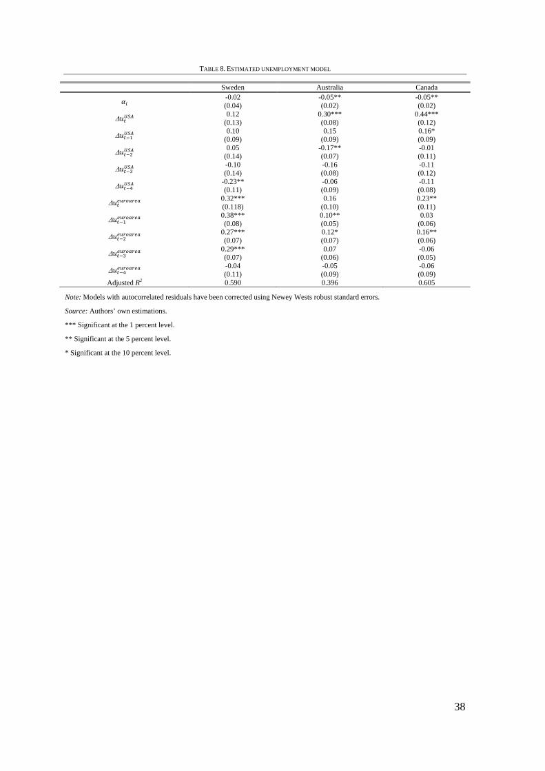
38

TABLE 8. ESTIMATED UNEMPLOYMENT MODEL

Sweden Australia Canada

-0.02 (0.04)

-0.05** (0.02)

-0.05** (0.02)

0.12

(0.13) 0.30*** (0.08)

0.44*** (0.12)

0.10

(0.09) 0.15

(0.09) 0.16* (0.09)

0.05

(0.14) -0.17** (0.07)

-0.01 (0.11)

-0.10 (0.14)

-0.16 (0.08)

-0.11 (0.12)

-0.23** (0.11)

-0.06 (0.09)

-0.11 (0.08)

0.32*** (0.118)

0.16 (0.10)

0.23** (0.11)

0.38*** (0.08)

0.10** (0.05)

0.03 (0.06)

0.27*** (0.07)

0.12* (0.07)

0.16** (0.06)

0.29*** (0.07)

0.07 (0.06)

-0.06 (0.05)

-0.04 (0.11)

-0.05 (0.09)

-0.06 (0.09)

Adjusted R2 0.590 0.396 0.605

Note: Models with autocorrelated residuals have been corrected using Newey Wests robust standard errors.

Source: Authors’ own estimations.

*** Significant at the 1 percent level.

** Significant at the 5 percent level.

* Significant at the 10 percent level.

39

TABLE 9. AVERAGE ANNUAL CPI-INFLATION AND GDP PER CAPITA GROWTH DURING FIVE MONETARY POLICY REGIMES

CPI-inflation GDP / capita Gold standard, 1873-1913 0.4 1.8 Interwar years, 1920-38 -2.3 3.0 Bretton Woods, 1951-73 4.7 2.9

Accommodation policy, 1974-92 8.4 1.3 Inflation target, 1995-2013 1.4 2.1

40

Appendix 1

Time series Data source

Inflation

CPI Andersson, Palmqvist and Österholm (2012) and

Statistics Sweden.

CPIF Andersson, Palmqvist and Österholm (2012) and

Statistics Sweden.

Perceived inflation NIER

United States CPI Thomson Reuters Datastream. Code:

USCONPRCE

Euro area HICP Thomson Reuters Datastream. Code: EMCPHARMF

Expected inflation

Employers’ and labour organisations’

expectations

TNS Sifo Prospera

http://www.prospera.se/

Households’ expectations NIER

Firms’ expectations Inflation report 2003:4 and Monetary policy

report, October 2013

Equilibrium Unemployment

NIER NIER 2013

The Riksbank Monetary policy report October 2010

UC, UC-trend and SVAR estimates of the

Riksbank Monetary policy report, July 2012

OECD OECD.stat

Unemployment

Unemployment, Sweden, old method Monetary policy report, July 2012

Unemployment, Sweden, new method Monetary policy report, February 2013

Unemployment, euro area Thomson Reuters Datastream. Code:

EKESUNEMO

Unemployment, USA Thomson Reuters Datastream. Code:

USUN%TOTQ

Unemployment, Australia Thomson Reuters Datastream. Code:

AUUN%TOTQ

Unemployment, Canada Thomson Reuters Datastream. Code:

CNUN%TOTQ

GDP / capita 1873-1992. Schön L and O Krantz (2012).

41

1993-2013. Statistics Sweden

Real unit labour cost

Real unit labour cost. Thomson Reuters Datastream. Code:

SDESF2W8h

Note: Monthly data has been converted to quarterly by taking the average over the monthly observations.