the residential pattern of military personnel associated
TRANSCRIPT

University of Nebraska at Omaha University of Nebraska at Omaha
DigitalCommons@UNO DigitalCommons@UNO
Student Work
7-1-1971
The residential pattern of military personnel associated with The residential pattern of military personnel associated with
Offutt Air Force Base, Nebraska, 1970 Offutt Air Force Base, Nebraska, 1970
Donald C. Rundquist University of Nebraska at Omaha
Follow this and additional works at: https://digitalcommons.unomaha.edu/studentwork
Recommended Citation Recommended Citation Rundquist, Donald C., "The residential pattern of military personnel associated with Offutt Air Force Base, Nebraska, 1970" (1971). Student Work. 673. https://digitalcommons.unomaha.edu/studentwork/673
This Thesis is brought to you for free and open access by DigitalCommons@UNO. It has been accepted for inclusion in Student Work by an authorized administrator of DigitalCommons@UNO. For more information, please contact [email protected].

THE RESIDENTIAL PATTERN OF MILITARY PERSONNEL ASSOCIATED WITH OFFUTT AIR FORCE BASE,
• NEBRASKA, 1970
A Thesis Presented to the
Department of Geography-Geology and the
Faculty of the Graduate College University of Nebraska at Omaha
In Partial Fulfillment of the Requirements for the Degree
Master of Arts
byDonald C, Rundquist
July, 1971

UMI Number: EP73313
All rights reserved
INFORMATION TO ALL USERS The quality of this reproduction is dependent upon the quality of the copy submitted.
In the unlikely event that the author did not send a complete manuscript and there are missing pages, these will be noted. Also, if material had to be removed,
a note will indicate the deletion.
Dissertafen Publishing
UMI EP73313
Published by ProQuest LLC (2015). Copyright in the Dissertation held by the Author.
Microform Edition © ProQuest LLC.All rights reserved. This work is protected against
unauthorized copying under Title 17, United States Code
ProQuest'ProQuest LLC.
789 East Eisenhower Parkway P.O. Box 1346
Ann Arbor, Ml 48106-1346

Accepted for the faculty of The Graduate College of the University of Nebraska at Omaha, in partial fulfillment of the requirements for the degree Master of Arts.
Graduate Committee
Chairman
Department

ii
ACKNOWLEDGEMENTS
The author is deeply indebted to Dr. Harold J. Retallick for his part in the preparation of this thesis. Dr. Retallick*s advice, assistance, professionalism, patience, and understanding are sincerely appreciated .
Others also played vital roles in the realization of this work.The assistance and inspiration of Mr. Chris L. Jung, especially in the early stages of the paper, are appreciated. Mr. Lee C. Bush donated much of his time to assisting the author with the computer applications, and he, too, deserves much thanks, Mr. Charles R. Gildersleeve rendered , assistance with the statistical techniques, and his efforts are appreciated.
Thanks is also expressed to the personnel of the Computer Center of the University, of Nebraska at Omaha, and to the many persons at Offutt Air Force Base who were so helpful.
iii
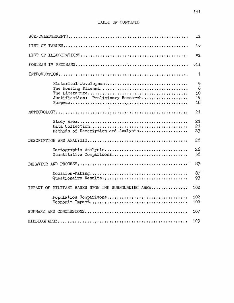
TABLE OF CONTENTS
ACKNOWLEDGEMENTS........... iiLIST OF TABLES.......................................... ivLIST OF ILLUSTRATIONS........... viFORTRAN IV PROGRAMS....................'....................... viiINTRODUCTION.................................................. 1
Historical Development............................... ^The Housing Dilemma...................... *......... 6The Literature....................................... 10Justifications Preliminary Research............. 1^Purpose........... 18
METHODOLOGY..................... 21Study Area............... 21Data Collection. ..................... 21Methods of Description and Analysis.................. 23
DESCRIPTION AND ANALYSIS...................................... 26Cartographic Analysis................................ 26Quantitative Comparisons ........................ $6
BEHAVIOR AND PROCESS...... 87Decision-Making................. 8?Questionaire Results ........ 93
IMPACT OF MILITARY BASES UPON THE SURROUNDING AREA.............. 102Population Comparisons.......... 102Economic Impact...................... 104
SUMMARY AND CONCLUSIONS........................ '........ 107BIBLIOGRAPHY................................ 109

iv
LIST OF TABLES
Table PageI. Housing Units vs. Military Personnel, 1965-1970............ 8II. Air Force Rank Structure..................... 9
III. Officer Totals by City and Town............. *..... 28IV. Percentage Totals for Each City and Town by Officer Rank.... 29V. Percentage of All Officers in Each City or T o m ....... 38VI. Enlisted Totals by City and Town ................ 40
VII. Percentage Totals for Each City and Town by Enlisted Rank... 41VIII. Percentage of All Enlisted Men in Each City or Town........ 53IX. Number and Percentage of All Offutt Servicemen in Each City
or Town. ............................... 54X. Comparison of Mean Centers............. *................. 60XI. Average Distance From Offutt.......... 64XII. Standard Distance Deviations.......... 68XIII. Number of Each Rank per Zone...................... 71XIV. Percentage of Each Rank per Zone.......... 72XV. Percentage of Each Rank per SDD.............. 73
XVI. Mean Distances: Actual vs. Expected...... 81XVII. Total Randomness Indices and Total Deviations.............. 83
XVIII. Regression Analysis ................ 86XIX. Officer and Airman Pay Scales .................... 90XX. Housing Types Selected by Offutt Personnel ... 9i
XXI. Number of Responses by Rank................ 96
XXII. Reasons Given for Residential Location Choice............... 97XXIII. Reasons Cited Under "Other" Response........... 99

V
Table PageXXIV. Home Community of Respondents............................ 100XXV. Housing Types of Respondents. ........... 101
vi
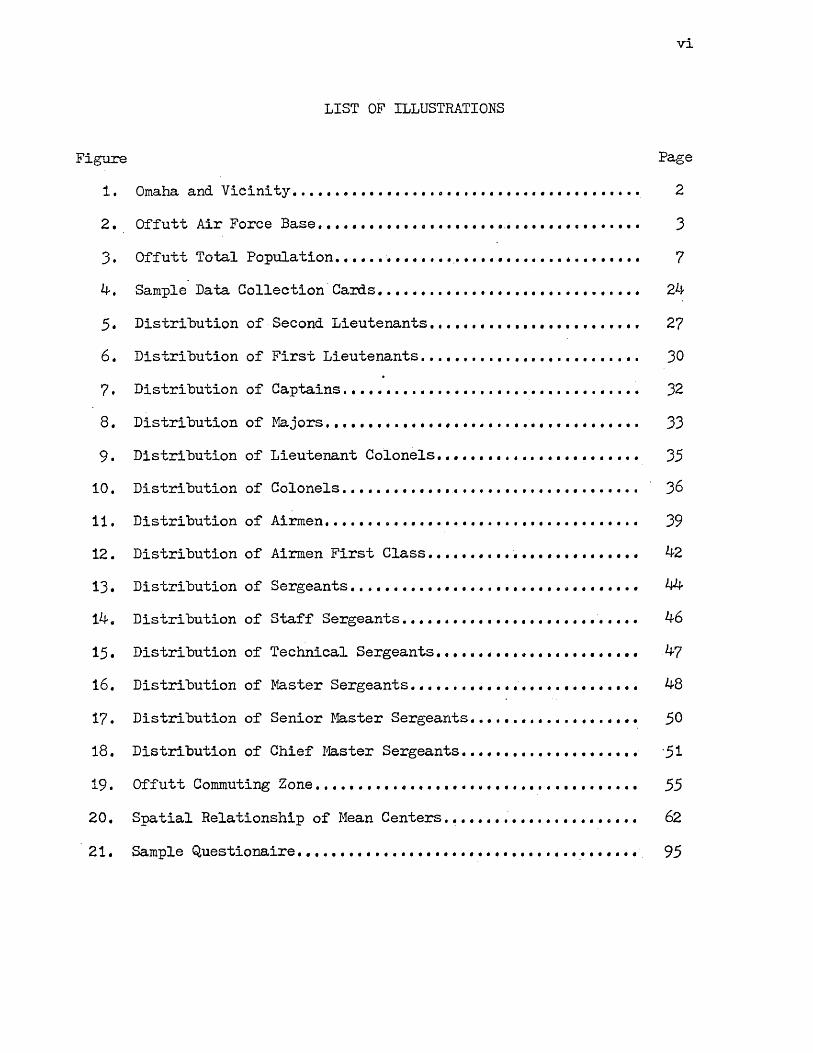
LIST OF ILLUSTRATIONS
Figure Page1. Omaha and Vicinity ........ 22. Offutt Air Force Base..................... 33. Offutt Total Population . •..... *....... 74. Sample Data Collection Cards........... 245. Distribution of Second Lieutenants.................. 276. Distribution of First Lieutenants......................... 307. Distribution of Captains.................................. 328. Distribution of Majors ....... 339. Distribution of Lieutenant Colonels.. ...... 3510. Distribution of Colonels............ ' 36
11. Distribution of Airmen............ 3912. Distribution of Airmen First Class 4213. Distribution of Sergeants... 4414. Distribution of Staff Sergeants. .............. 4615. Distribution of Technical Sergeants ....... 4716. Distribution of Master Sergeants. ......... 4817. Distribution of Senior Master Sergeants ..... 5018. Distribution of Chief Master Sergeants. . -51
19. Offutt Commuting Zone.................................... 5520. Spatial Relationship of Mean Centers.. ............. 6221. Sample Questionaire........ 95
vii
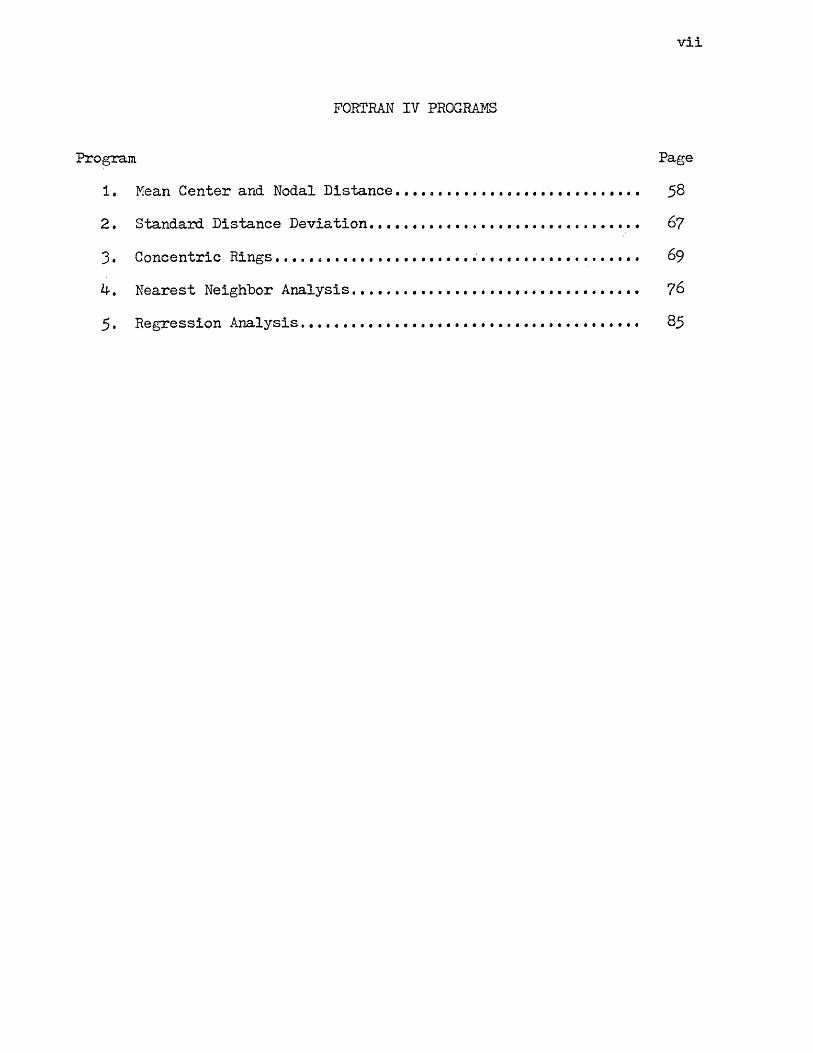
FORTRAN IV PROGRAMS
Program Page1. Mean Center and Nodal Distance.............. 58
2. Standard Distance Deviation.............................. 67
3. Concentric Rings....................... 69
Nearest Neighbor Analysis.................. 76
5 . Regression Analysis...................................... 85

INTRODUCTION
"A particular method of inspecting data is known to all scholars as the geographic method, based on charting the limits or range of phenomena, features, or traits that have a localized distribution on the earth."* Geographers have long been concerned with the distribution of phenomena, whether they be species of trees, refugees, cities, land use, resources, glaciers, farms, ethnic groups, religions, or a myriad of other examples, and distributional analyses are fundamental to the discipline of geography. During the infancy of geography as a discipline, the studies of distributions were mainly descriptive, but as the subject grew and became, more sophisticated, comparison with other patterns and explanation became important. As Taaffe has noted, the geographer still describes and analyzes patterns found on maps, but behavior and process are becoming important considerations.̂ This paper, too, is designed to study the patterns found on maps, that is, the residential patterns associated with the military personnel of Offutt Air Force Base, Nebraska, Process is also one of the considerations .
At the end of the working day, thousands of automobiles leave the four gates of Offutt Air Force Base, a i,907-acre installation near Omaha, Nebraska (Figures 1 and 2), and begin the trek toward several of the base’s "urban dormitories. Air Force people are an integral
Carl Sauer, "The Education of a Geographer," in Land and Life, edited by John Leighly, Berkeley: University of California Press,1967. p. 39^.
^Edward J. Taaffe (ed.), Geography* Englewood Cliffs, N.J.: Pren-tice-Hall, Inc., 1970, p. 8.

2
OfVIAHA AMD V8CSMBTY
AV'a m e s
CARTER LAKE V?
(IOWA) /
BLONDO
OMAHABOYSTOWN WEST BROADWAY
STPOPS
COUNCILBLUFFS
ST
[ALSTON
/ D O UGLAS- - - - - - IOWACHANDLER NEBRASKA
CHILPSX \R DIGILES RD
IELLEVUEAPILLi
HWX.
SCALE IN MILES FIGURE 1

3

If
part of the Omaha-Council Bluffs, Iowa, metropolitan area, and most of the civilians have had. some contact with the military individual, whether in one*s neighborhood, the schools, church, or just a casual meeting on the street. This phenomenon, the military base and Its relationship to a civilian community, offers many possibilities for - research. This thesis, however, is concerned with only one, the location of the residences of Offutt*s personnel with respect to individual rank, and possible reasons for their choices.
Historical Development
Offutt Air Force Base, Headquarters for the Strategic Air Command since its inception in 19^3, has a long history, dating back to July 23, 1888, when the United States Congress and President Cleveland authorized the purchase of land for an Army post, and appropriated $ 2 0 0 , 0 0 0 . 3 In 1891, President Harrison directed that the new fort be named in honor of Major General George Crook, and on June 28, 1896, the first four companies of the U.S. Army Infantry arrived. During the Spanish- American War-, Fort Crook was a recruiting center and way station for troops on their way to Cuba, and later, the Philippines.
Fort Crook acquired its first air power in 1918 with the arrival of the 61st Balloon Company, a combat reconnaissance unit. The first dirt runways and steel hanger were completed by 1921, and two DeHaviland DH-^B’s began carrying mail from the post. In 192^, the air field
^For the historical discussion, reference is made to "A Chronology of Offutt Air Force Base," Offutt Air Force Base Publication 210-1-1, and "Offutt Air Force Base and SAC Headquarters Base Guide, 1969-1970," Published by Sun Newspapers, Omaha, Nebraska.

5
portion of Fort Crook was renamed "Offutt Field," in honor of First Lieutenant Jarvis J. Offutt, Omaha*s first air casualty of World War I.
About 500 acres and all flying facilities were leased to the Martin Bomber Company in 19M for the construction of a bomber plant, which reached full-scale production about one year later* Also during World War II, Fort Crook was a Prisoner of War camp for Italian prisoners.
In 19^6# Fort Crook was transferred to the Army#s Second Air Force, and the entire installation was renamed Offutt Field, The total strength of the post in late 19^7 was 7^5 military, and 3^0 civil service employees,
Offutt Field was transferred to the newly-created Department of the Air Force in January of 19^8, and m s renamed "Offutt Air Force Base," It became the Headquarters for the Strategic Air Command (hereafter referred to as SAC) later in the same year.
Today, Offutt is the home of four Air Force Wings; 3902nd Air Base Wing, 3x& Weather Wing, 5^4th Aerospace Reconnaissance Technical Wing, and the 55th Strategic Reconnaissance Wing,^ The 3902nd is the administrative and operational support wing for Offutt, 3rd Weather operates Global Weather Central for SAC, the 5^th is one of SAC8s primary intelligence units, and the 55th SRW’s mission is reconnaissance and to maintain the Airborne Command Post, "Looking G l a s s , Other units assigned to Offutt include the 1st Aerospace Communications Group,
^A wing is composed of four or more squadrons, (two or more groups), and can operate as an independent unit without outside support,
5ln the event the SAC underground command post and the alternate command posts are destroyed, the "Looking Glass" aircraft, an EC- 135Stratotanker, can assume command of SAC,

6
1911 Communications Squadron, ^27 Field Training Detachment, and the British Royal Air Force Detachment (Strike Command RAF).
The Housing Dilemma
The military and civilian population of Offutt Air Force Base has continued to increase through the years (Figure 3), and overcrowded Base housing first "became a problem during the 1950®s, when many on- base housing projects were begun.6 Housing was Offutt9s most critical problem in i960, as there were only 832 government units available, with an estimated 6,169 families requiring housing. The total personnel assigned to Offutt in I960 was over 10,000, with an additional 159000 dependents,? Government housing construction continued through the 1960cs, with many projects reaching completion. For a comparison of the I965-I97O period, consult Table I on page 8. From this table, it . can be seen that the total military strength in 1970 was 12,239* It is interesting to note that the available barracks space at this time was 3,22^, but the barracks were only 72% occupied. This is an indication that many of the single Airmen (Sergeants, E-4, and above) have chosen to move off the base, and find housing elsewhere (for rank comparisons, see Table II).®
It can easily be seen from the above' figures that on-base federal family housing cannot possibly accommodate all of the Offutt personnel, and many are forced to find housing within the surrounding communities,
£°The source of Figure 3 is James Bresette, "Omaha and Offutt Spur Sarpy." Omaha World-Herald. September 239 1970* P* 23*
?"A Chronology of Offutt Air Force Base,” on. cit.®In order to reside off-base, an enlisted man must be a Sergeant
(E-4) or above, or else married. Any Officer can live off-base.

L .................... .... .. ... j , .......
1950 1955 1960 1965Y©ars
— 1 1970
F l @ U i E 3,

8
TABLE IHOUSING UNITS VS. MILITARY PERSONNEL, 1965-1970
Year Number of Housing Units Militarv Pers-
1965 2,102 9*7651966 2,09^ 10,w1967 2,202 9,8881968 2,381 10,7951969 2,381 10,935*1970 2,381 12,239*
^Indicates strength for the specific day of December 25. All other figures are the average for the month of December.Data courtesy of SSgt Kermit Cox, Offutt Air Force Base Information Office.

9
TABLE II AIR FORCE RANK STRUCTURE
Grade Rank Name Abbreviation*E-l Airman Basic ABE-2 Airman ArnnE-3 Airman First Class A1CE—4 Sergeant SgtE-5 Staff Sergeant SSgtE-6 Technical Sergeant TSgtE-? Master Sergeant MSgtE-8 Senior Master Sergeant SMSE-9 Chief Master Sergeant CMS
Warrant Officer WO0-1 Second Lieutenant 2Lt0-2 First Lieutenant ILt0-3 Captain Capt0-4 Major Majo-5 Lieutenant Colonel LC0-6 Colonel Col0-7 Brigadier General BG0-3 Major General MG0-9 Lieutenant General LG0-10 General Gen
*Used in some of the tables and figures in the text.

10
although some do so by personal preference. It is this dispersion of military personnel into the civilian populace with which this thesis is concerned, and it is a geographic problem of large proportion.
The Literature
An extensive review of the geographic literature indicates a scarcity of work done on distributions of military personnel within a civilian community. One unpublished study, by David B. Cole of the United States Air Force Academy, has dealt with a problem similar to that of this t h e s i s *9 Cole, studying Lowry Air Force Base, Denver, Colorado, originally hypothesized that Air Force families tend to cluster in a civilian community, and considered factors influencing the decisionmaking that led to the observable residential patterns. From a random sample of 365 Air Force families, he found no evidence of rank segregation in housing patterns, and suggested that the Air Force structure breaks down in neighborhood groupings in a civilian community.Cole did find some evidence of clustering, however, in the inner-city, where mostly enlisted men lived, due to the lower rents. He used Nearest Neighbor Analysis in describing his distribution, which refuted the original hypothesis, as only one of the six areas of Denver that were studied had an "R” value (index of randomness) that inferred clustering. The other five had R values inferring a uniform distribution of Air Force families. As a complementary hypothesis, then, Cole suggested
^David B . Cole, "Military Residential Patterns in a Civilian Community," Presented at the Annual Meeting, Great Plains-Rocky Mountain Division, Association of American Geographers, U.S. Air Force Academy, Colorado Springs, Colorado, October, 1970.

ii
that those who live off-base generally desire greater interaction with the civilian community, and, therefore, resist military clustering.
Cole used an open-ended questionaire in studying the decisionmaking process of residential choice, and found that the joumey-to- work was an important consideration to Air Force people. Most families preferred a 10 to 15 minute drive to the base. Many planned to retire in the area of Denver, and considered this in their choice of residence. Nearness to schools was another important consideration by most.
Tito relatively recent geography Masters Theses have studied problems of cities and their relationship to military installations. R.H. Pietz investigated the economic impact of the Cherry Point (North Carolina) U.S. Marine Corps Air Station upon the local settlement.10 Residential patterns are not discussed in detail, but the author notes that the Cherry Point marines tend to live near the base, while the civilian workers tend to commute at least 20 miles. He attributes this to the fact that the marines are expected to respond to national emergencies, and can better do so from a nearby residential position. Also, the marines are more accustomed to the aircraft noise-nuisance.
Louise K. Monaghan studied Warner Robins Air Force Base in relation11to the adjacent city of Warner Robins, Georgia. This work is largely
an historical account of the city growth as a result of the military
^Reuel H. Pietz, "The Impact of the Cherry Point Marine Corps Air Station Upon Local Settlement," Unpublished Masters Thesis, East Carolina College, 1964.
ilLouise K. Monaghan, "Military Bases as Nuclei for Urbanization: Warner Robins, Georgia," Unpublished Masters Thesis, University of Tennessee, 1968.
12
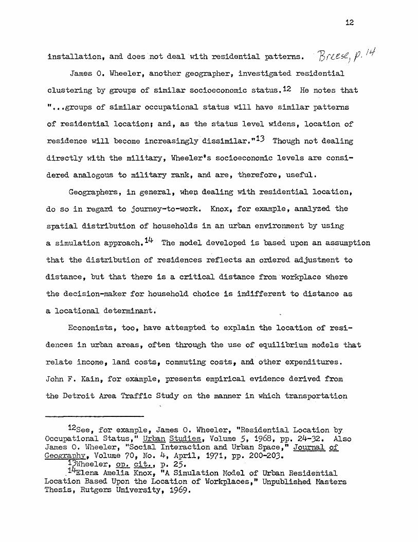
installation, and does not deal with residential patterns. p . ^
James 0. Wheeler, another geographer, investigated residential clustering hy groups of similar socioeconomic status.12 He notes that "...groups of similar occupational status will have similar patterns of residential location; and, as the status level widens, location of residence will become increasingly d i s s i m i l a r . " ^ Though not dealing directly with the military, Wheeler*s socioeconomic levels are considered analogous to military rank, and are, therefore, useful.
Geographers, in general, when dealing with residential location, do so in regard to joumey-to-work. Knox, for example, analyzed the spatial distribution of households in an urban environment by using a simulation approach.^ The model developed is based upon an assumption that the distribution of residences reflects an ordered adjustment to distance, but that there is a critical distance from workplace where the decision-maker for household choice is indifferent to distance as a locational determinant.
Economists, too, have attempted to explain the location of residences in urban areas, often through the use of equilibrium models that relate income, land costs, commuting costs, and other expenditures.John F. Kain, for example, presents empirical evidence derived from the Detroit Area Traffic Study on the manner in which transportation
^See, for example, James 0. Wheeler, "Residential Location by Occupational Status," Urban Studies. Volume 5, 1968, pp. 2^-32. Also James 0. Wheeler, "Social Interaction and Urban Space," Journal of Geography, Volume 70, No. April, 1971, pp. 200-203.
3»3wheeler, on. cit.. p. 25.,̂ -TElena Amelia Knox, "A Simulation Model of Urban Residential
Location Based Upon the Location of Workplaces," Unpublished Masters Thesis, Rutgers University, 1969.

13
costs influence residential location.^ The hypothesis of his residential location model, supported by the Detroit data, is that households substitute journey-to-work expenditures for rent. Ira Lowry*s model considers adequate site space for domestic activities to be of equal importance with commuting costs.16 Models proposed by Alonso and Wingo appear to be similar in attempting to explain residential location.17
Sociologists are active in residential pattern research, and, like the economists, tend to view residential location as a function of the joumey-to-work. J. Douglas CarrQll, after a study of over 72,000 industrial, workers, stated in 19^9> "We have established evidence of the tendency on the part of workers to minimize the distance between home and w o r k . " 18 He noted in 1952 that the result "...is an important factor conditioning total residential, arrangement of urban populations19 Loewenstein, too, views workplace as an important factor in the spatial distribution of residences, as the household head attempts to minimize his journey-to-work.^O other sociologists, such as the Duncan*s, relate
15John F. Kain, "The Journey to Work as a Determinant of Residential Location," Papers and Proceedings of the Regional Science Association. Volume 9s 1962, pp. 137-160.
l6lra S. Lowry, A Model of Metropolis, Santa Monica: The RandCorporation, 1964.
l?William Alonso, Location and Land Use: Toward a General Theoryof Land Rent, Cambridge: Harvard University Press, 1964. Also LowdonWingo, Transportation and Urban Land. Washington, D.C.: Resources forthe Future, Inc., 1961.
18J. Douglas Carroll, Jr., "Some Aspects of the Home-Work Relationships of Industrial Workers," Land Economics, Volume 25» No. 4, November, 1949, pp. 414-422 (quoted statement, p. 422).
I7J. Douglas Carroll, Jr., "The Relation of Homes to Work Places and the Spatial Pattern of Cities," Social Forces. Volume 30> March,1952, p. 271.
2°Louis K. Loewenstein, "The Industry of Employment: A NeglectedFactor in the Spatial Distribution of Residences in Urban Areas," American Journal of Economics and Sociology. Volume 24, No. 2, April, 1965* pp. i57~l62. Also Louis K. Loewenstein, The Location of Residences and Work Places in Urban Areas. New York: The Scarecrow Press, Inc., 1965.

14
socioeconomic status to residential s e g r e g a t i o n . ^
Gerald Breese, Bureau of Urban Research, Princeton University, collaborating with several co-authors, has produced a large volume dealing with the impact of large industrial and military installations upon nearby a r e a s . ^2 One of the five case studies investigates Dover Air Force Base, Delaware, after its reactivation in 1952.^ The distribution of Air Force families was studied using a 5Q?o sample, and one result m s that the military tend to live as close as possible to the base. The survey indicated that 8 ^ of the military families live within ten miles of the base, but analyses by individual rank were not undertaken.
One can note that specific works are few, but there are some general sources available. Little work has been done within the field of geography with regard to military distributions, and none have studied distributions by individual rank. It seems safe, then, to label this thesis as "basic research."
Justification: Preliminary Research
Is there a problem to be resolved in regard to Offutt Air Force Base, and if so, is it a justifiable one? The author completed a preliminary study on the subject of Offutt9s off-base residential patterns
p 4^ See, for example, Otis D. and Beverley Duncan, "Residential Distribution and Occupational Stratification," found in Paul K. Hatt and Albert Reiss (eds.), Cities and Society, Glencoe, Illinois: TheFree Press, 1959•
22Gerald Breese, et al, The Impact of Large Installations on Nearby Areas, Beverly Hills: Sage Publications, Inc., 19&5*
23The author of the Dover study is Lt. James E. Whelan, CEC, USN.

15
in the Fall of 1969. ^ This smaller paper utilized August 30, 19&9»
data for all 2,559 Officers assigned to Offutt at that time, and September, 1969t data for a sample (1,871) of the enlisted personnel.The source material from 'which the addresses were extracted was of a lesser caliber than that used for this thesis, but it did prove useful. The Officer addresses were derived from the base Officer Information Directory, a compilation of all Officers assigned to Offutt.^ A sample of the enlisted personnel was taken from the Roster of Enlisted P e r s o n n e l . 26 This immense volume was somewhat incomplete, but did allow some comparison with the Officers.
It should be noted that the unit of analysis for this preliminary research was the 1970 Census Tract. After this initial attempt, the author concluded that the Census Tract was inadequate, as the desired precision in plotting was lacking using a unit of analysis and mapping chloroplethically. Some of the findings of the earlier work that led to this thesis are, however, deemed worthy of mention at this time.
In studying the Officers, the author eliminated those that lived on-base in federal housing or barracks, as well as those for whom no address was given in the Officer Information Directory. From the original 2 ,559, then, 1,507 valid addresses remained, and were plotted within the Census Tracts. No other refinement of location was made,
^Donald C. Rundquist, ’’The Distribution of Military Personnel Around Offutt Air Force Base, Nebraska," Unpublished Research Paper, University of Nebraska at Omaha, January, 1970.
25Officer Information Directory. Headquarters Strategic Air Command and Offutt Air Force Base, Nebraska, August 30, 19&9*
26Rgster of Enlisted Personnel. Offutt Air Force Base, Nebraska, September, 1969. Obtained through the courtesy of the Offutt Air Force Base Transition Office,
16
and mapping was, as already mentioned, chloroplethic.One important finding of the preliminary paper was the "rank-
progression,” or pattern, and it was noted that in the case of Bellevue, as rank declined, the percentage of each Officer rank in Bellevue also declined, while the percentage in Omaha generally increased. Whereas £&.3% of all Colonels living off-"base chose Bellevue for residence,75% of the Lieutenant Colonels, 67>2% of the Majors, 6̂ .3% of the Captains, 65»3% of the First Lieutenants, and 6l.5% of the Second Lieutenants chose that same city. No/ting Officers in Omaha, it was found that 7*8% of the Colonels, 12.2% of the Lieutenant Colonels, 10.2% of the Majors, 17*3% of the Captains, 21,2% of the First Lieutenants, and 2J% of the Second Lieutenants selected that city. Finally, there was a higher percentage of Majors and Captains living in Papillion than any other rank, so one can readily see that there are perceptible patterns reflected in these percentages.
When the percentage of all Officers in each city or town was con- • sidered, there was an overwhelming majority in one city. Bellevue contained 67 *2% of all the Officers that lived off-base, while Omaha had 1^.7%, and Papillion was third with 13 A%, . The remaining towns containing Officers had only 1% or less of the total.
The rank-progression was not as ordered in the case of the Airmen, but some patterns were evident. The enlisted statistics were compiled from four representative squadrons, two rather large, and two small.27 All of the enlisted men within these organizations were considered.
27 a squadron is the basic administrative unit of the Air Force.It is a group of men organized under a commander to perform a specific function.

17
One problem, though, was the 'large number of men for whom no address was given in the Roster of Enlisted Personnel. After culling these from the total sample, only 434 valid addresses remained, but they do offer some insight into the enlisted residential distribution.
The Omaha percentages, from the rank of Master Sergeant through Airman First Class, begin to hint at a pattern, with 26,5% of the Master Sergeants, 40,*1% of the Technical Sergeants, 45.9^ of the Staff Sergeants, and 53 'V% of the Sergeants living off-base, choosing Omaha. Airman First Class was not a part of the progression, with a percentage of 40.4. Bellevue's enlisted figures, showed that 6l,&% of the Master Sergeants, 5k *6$% of the Technical Sergeants, 32.6% of the Staff Sergeants, 36 ,Wo of the Sergeants, and 48.9% of all Airmen First Class reside in that city, The ranks of Chief Master Sergeant, Senior Master Sergeant, and Airman are not included in this discussion since too few addresses were available to insure validity.
A much more diversified distribution was noted for the Airmen than the Officers in the preliminary study. Whereas for Officers, only three cities had percentages above 1% (Bellevue, Omaha, and Papillion), the enlisted exceeded 1% in six communities (Omaha, Bellevue, Plattsmouth, Council Bluffs, LaVista, and Papillion). The enlisted figures, too, showed no overwhelming majority in any one city, with 44.7% in Omaha, 38.7% in Bellevue, 6,6$% in Plattsmouth, 5*6$% in Council Bluffs, 2 ,Wo in LaVista, and 1.6% in Papillion. Therefore, it seemed that the enlisted personnel tended to disperse to a greater degree. These were the main findings of the preliminary research, which was designed to test the validity of the original idea for the thesis.

18
There were some inconsistencies in the original research which have been adjusted in the thesis. One of the most prominent was the need for a more precise designation of particular city. In the preliminary study, for example, if a person lived outside the Omaha city limits but had an Omaha mailing address, he was considered a part of the Omaha total. Much more exact labeling is utilized in the thesis, and to be included in the Omaha total (or any city’s statistics), one has to actually live, within the city limits. Also, the enlisted sample was very small in terms of the total enlisted personnel at Offutt, and the data source was not complete, or kept totally current. Both of these problems have been rectified, since the total population of Offutt is examined in the thesis, and the data source is very accurate. Though there were some problems in the preliminary study, it certainly identified a distribution problem, and attested to the validity, warranting investigation in much greater detail.
Purpose
As Cole noted in the study of Lowry Air Force Base and the Denver environs, "The choice of residence is a behavioral process which is often part of a larger spatial pattern bearing certain definable relationships. Many regularities are evident in the distribution of military residences, as will be seen later in this thesis. Cole’s original hypothesis (refer to page 10), although disproven, stated that residences of Air Force families tend to cluster in a civilian
28Cole, op. cit.. p. 1.
19
c o m m u n i t y .29 This study advances that hypothesis one step further, proposing that the military rank of the individual is very important in residential location, and that there are residential clusters according to rank. The author also suggests that rank plays a role in the type of housing selected; apartment, single-family, or trailer, as well as the distance traveled to work.
The first obligation of the geographer is to deal with the concept of "where." Exactly where do the Offutt Air Force Base personnel live?. There are certainly several secondary or allied problems associated with this thesis, but the cartographic representation of the spatial distribution of the off-base residential locations of all Offutt military personnel, and the associated quantitative applications, are of prime importance.30 Most of the local citizenry, as well as the military personnel themselves, have vague notions as to where most of the Air Force people reside in and around the Omaha area, but no work, to the knowledge of this writer, has discussed this large military distribution in exact terms.
While the mapping and quantitative measures comprise the main
29Ibid.30Generals, Warrant Officers, Airmen Basic, and OSI Special Agents
are generally ignored in this paper, for various reasons. All Generals live in government housing, so they are unimportant to the study. Warrant Officer is a dying rank, as the Air Force is eliminating it. A Warrant Officer is a former enlisted man who had been promoted to an Officer grade, but ranks below a Second Lieutenant. There are only a few Warrant Officers at Offutt, and most live in government housing. Airmen Basic are also excluded from the thesis since there are only 4 living off-base (3 in Omaha and 1 in Fremont). Airmen Basic (E-l) are usually disciplinary cases, since all new enlisted men are automatically awarded the rank of Airman (E-2) upon completion of basic training. The ranks of the OSI Special Agents (roughly analogous to a military FBI) are kept classified, so these men cannot be studied in terms of residential location.
20
intention of the thesis, the author notes other features inherent in the problem, such as the types of housing generally chosen by certain ranks, distances traveled (thus establishing a "Commuting Zone" for Offutt), some comparisons of clusters of military and the transportation arteries (as each rank distribution is discussed), and a brief discussion of the considerable economic impact of Offutt Air Force Base on the Omaha area. A most important question, too, will be deliberated, that is, why do these individuals choose to settle where they.do?The analysis of this question is.based upon the results of a question- aire circulated at random by the author during late 1970 at Offutt.

21
METHODOLOGY
Study Area
When the original idea for this thesis was conceived, some thought was given to using a specific area of study, such as the Omaha Standard Metropolitan Statistical Area, and noting military residential patterns within that unit. Granted, this division would include most of Offutt°s personnel, and would "be a valid study, hut this writer, in an effort to uncover the exact distribution, chose not to limit the study area in this manner. Hence, the geographic boundaries for this paper are unlimited, and are defined only by the maximum distance in all directions that an individual is willing to travel daily to Offutt for work. The Omaha urbanized area will, however, receive the most investigation since the bulk of the personnel live within that area.
Data Collection
In an attempt to map the military distribution with as much precision as possible, it was felt that the total population of the base should be used, rather than just a sample. With that decision, a search of Offutt facilities began for a composite, up-to-date listing of all military personnel on the base. This directory had to contain, at minimum, 'the rank and home address of each person. Logically, the search led to the Base Accounting and Finance Office, since this unit utilizes the required information in distributing the payroll checks. After an explanation of intent, the Finance Officer agreed to relinquish the January 7» 1970» edition of the Master File Listing:, a weekly

22
computer print-out.31 This is the most accurate listing found on the "base, as individuals make certain that the Finance Office has their correct rank and address to insure both the proper amount of pay and - receipt of the cheek. The Master File Listing contains the name, rank, and address of each military individual assigned to Offutt Air Force Base. The author m s fortunate to obtain these massive volumes that offer a wealth of information to the geographer. Without this directory, the study would have been much more difficult.
The first step in the solution of any problem is to collect the data, and, in this case, it proved to be a very formidable task. The author scrutinized approximately 16,600 enlisted names and addresses, and an additional 4,500 Officer entries, for a total of 21,100, From these, personnel living on the base in barracks or federal family-type housing were eliminated, as well as those individuals not assigned to Offutt.32 Only the rank of the personnel living on-base was recorded, and they were counted. Also eliminated were those persons having their payroll checks sent to their respective organizations (or squadrons). Some individuals pick up their checks personally at the Finance Office, and these, too, were eliminated. All of these eliminations were grouped in a category coded "SA" ("squadron address"), and counted for statistical purposes. One other example of an address noted only for, statistical reasons is "Box 19» Bellevue," Addresses such as these were
3*The print-out consists of two listings; one for Officers and one for Airmen.
32The personnel of such places as Ellsworth and Whiteman Air Force Bases, Scribner and Chandler Air Force Stations, and other small detachments that the Offutt Finance Office supports are also listed in the Master File Listing.

23
coded "Cl” ("cannot identify"), Also grouped in the "Cl" category, were those few addresses which could not be identified due to keypunch error, and the ones that simply could not be located. All other valid, normal addresses were recorded in the manner illustrated on page 2U-
(Figure *0.The method of noting the addresses on small cards was an effec
tive one for this problem. It allowed rapid sorting in many different ways, such as by rank, type of housing chosen, street, or city. Some thought was given to a keypunched. 80-column card for each entry, but accessibility to a keypunch machine at the time of data collection, as well as the time involved in keypunching that many entries and cards, tended to discourage further consideration of the method.
After all the pertinent data had been collected, each address had to be mapped.^ The mapping was done by using an acetate sheet for each rank, and placing it over the base map,3^ The finished maps utilize point data and proportional circles (point symbols). They are, therefore, quantitative.
Methods of Description and Analysis
After a map for a particular rank was completed, it was placed over a large sheet of arithmetic graph paper. The x and y coordinates for each point (or residence) were recorded, and later a card was key-
33phis process was facilitated by first sorting the addresses by rank, and then by streets, so all numbers on a given street for a certain rank could be mapped at one time.
3^he "Omaha and Vicinity" map, published by the Omaha City Planning Department, October 23$ 19&9» "was used as the base map. The date of this map corresponds closely with the date of the data, thus insuring validity.

SAMPLE DATA COLLECTION CARDS
.(Apartment) (Rank: 1
(Street Name) (Street Number) (City: Bellevue)
Galvin Rd. N. 202________
33 T-
Betz1100
.(Rank: 01=2Lt)
FIGURE k

25
punched,for each point. These x and y values are the foundation for several quantitative measures utilized in this thesis to aid in describing the distributions for each rank. The derivations include Mean Center, "Nodal Distance," Standard Distance Deviation* "Concentric Zone Analysis," Nearest Neighbor Analysis, and basic Linear Regression. All calculations were done by computer, utilizing the Fortran IV language.
The quantitative methods mentioned above allowed accurate description of the distributions in terms of the center of each, the dispersion or spread, numbers in zones away from the center, the index of randomness or general description of the distribution, and its alignment. Without statistical methods and computer applications, the large numbers of data studied in this paper would have been cumbersome, and the total population of Offutt could not have been analyzed in any detail.

26
DESCRIPTION AND ANALYSIS
Cartogra-phic Analysis
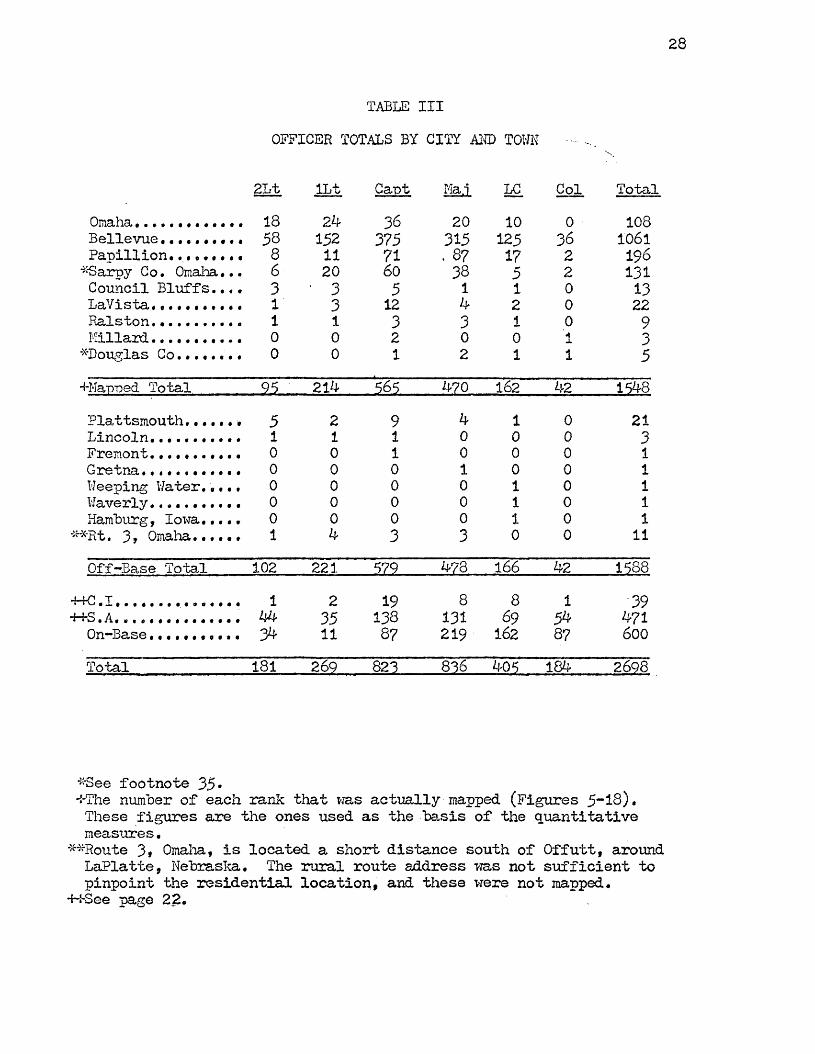
The homes of Air Force personnel are found in nearly all parts of the Omaha urbanized area, as well as other communities located some distance away from Offutt. All those living in the Omaha urbanized area were mapped, while those in communities farther away were recorded for statistical purposes, and the location of the community was mapped to aid in delimiting Offutt®s Commuting Zone.^-5 A total of 1,548 Officer and 2,474 enlisted residences were mapped (total, 4,022), and are recorded in Figures 5 through 18.
Considering Officers first, reference is made to Tables III and IV, in addition to Figures 5 through 10. Figure 5 illustrates the distribution of Second Lieutenants in and around Omaha. One can see some concentration along Galvin Road and Highway 73“75 in Bellevue, and the southern of Papillion.Each of these areas contains numerous apartment complexes. Table III lists 58 Second Lieutenants in Bellevue, which Table IV converts to 5^*86^.
Residences of First Lieutenants axe depicted in Figure 6. Again, there is some concentration in Bellevue along Galvin Road and Highway
3^The Omaha urbanized area is taken here to include Omaha, Bellevue, Papillion, Council Bluffs, LaVista, Ralston, Hillard, Carter Lake,"Sarpy County Omaha," and the immediate Douglas County area around Omaha. The label, "Sarpy County Omaha," was contrived by the author to describe that area south of Omaha in Saxpy County that appears to be more closely tied with Omaha than Bellevue, but is a part of neither.
38p0r reference to street names and the communities around Omaha that are mentioned in the text, refer to Figure 1, page 2. The communities not located in the immediate Omaha area are shown in Figure 19.
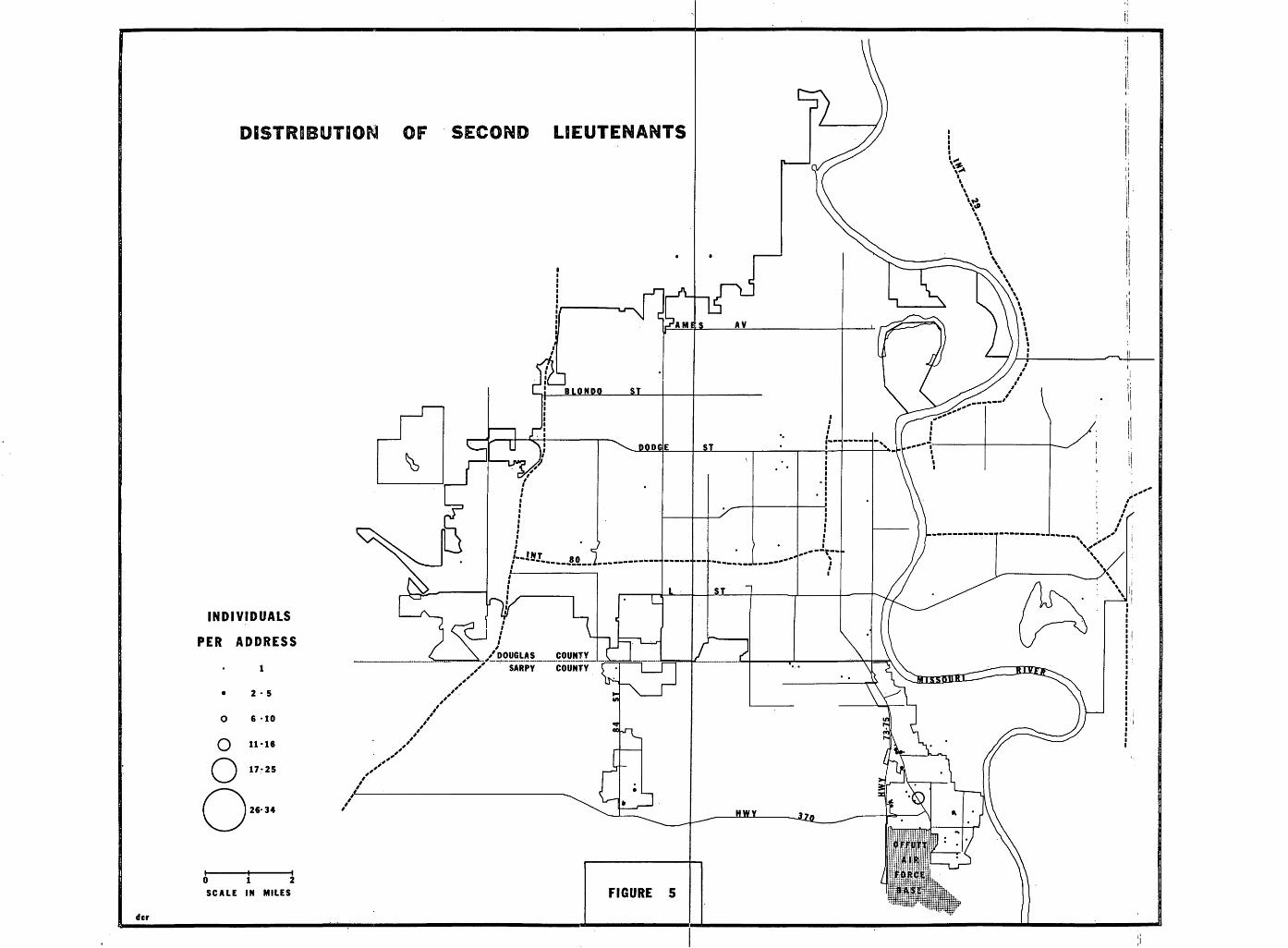
DISTRIBUTION OF SECOND LIEUTENANTS
AV
BLONPO 11
PODG
I ST
ST
INDIVIDUALS
PER ADDRESS/D O U G L A S COUNTY
SARPY COUNTY
6 10
17-25
26-34 H W Y
FIGURE 5S C A L E IN MILES
dcr
28
TABLE III OFFICER TOTALS BY CITY AND TOWN
2Lt lLt Cant Ma.i LC Col TotalOmaha............. 18 24 36 20 10 0 108Bellevue.......... 58 152 375 315 125 36 1061Paoillion......... 8 11 71 . 87 17 2 196“'•■Sarpy Co. Omaha... 6 20 60 38 5 2 131Council Bluffs.... 3 • 3 5 1 1 0 13LaVista. 1 3 12 4 2 0 22Ralston,.......... 1 1 3 3 1 0 9Millard........... 0 0 2 0 0 1 3^Douglas Co........ 0 0 1 2 1 1 5•fMa-p-ped Total_______ 95 214 565 470 162 42 1548Plattsmouth....... 5 2 9 4 1 0 21Lincoln........... 1 1 1 0 0 0 3Fremont........... 0 0 1 0 0 0 1G r e t n a 0 0 0 1 0 0 1Weeping Water....,0 0 0 0 1 0 1Waverly........... 0 0 0 0 1 0 1Hamburg, Iowa.. . . . 0 0 0 0 1 0 1
**Rt. 3, Omaha 1 4 3 3 0 0 11Off-Base Total 102 221 579 478 166 42 1588
++C.I 1 2 19 8 8 1 39++S.A............. 44 35 138 131 69 54 471On-Base........... 34 11 87 219 162 87 600Total 181 269 823 836 405 184 2698
*See footnote 35•*fThe number of each rank that was actually mapped (Figures 5~18). These figures are the ones used as the basis of the quantitative measures.
**Route 3, Omaha, is located a short, distance south of Offutt, around LaPlatte, Nebraska. The rural route address m s not sufficient to pinpoint the residential location, and these were not mapped.
•H-See page 22.

29
TABLE IVPERCENTAGE TOTALS FOR EACH CITY AND T O M BY OFFICER RANK
2Lt IL.tOmaha...... l? .6k 10.85Bellevue........ ■ 56.86 68.77Papillion....... ?.8k 4.97Sarpy Co. Omaha.. 5.88 9.04Council Bluffs... 2.94 1.35LaVista.......... 0.98 1.35Ralston. 0.98 0.45Millard......... 0 0Douglas Co....... 0 0Plattsmouth...... 4.90 0.90
Lincoln....•••••• 0.98 0.45Fremont......... 0 0Gretna........ 0 0Weeping Water.... 0 0Waverly...... 0 0Hamburg, Iowa.... 0 0Rt. J , Omaha..... 0 .98 1.80
Cant Mai LG Col6.21 4.18 6.02 0
64.76 65.89 75.30 85.7112.26 18.20 10.24 4.7610.36 ?. 94 3.01 4 ,760.86 0.20 0.60 02 .0 7 0.83 1.20 00.51 0.62 0.60 00.34 0 0 2 .380.17 0.41 0.60 2.381.55 0.83 0.60 00.17 0 0 00.17 0 0 00 0.20 0 00 0 0.60 00 0 0.60 00 0 0.60 00.51 0.62 0 0

DISTRIBUTION OF FIRST LIEUTENANTS
AV
IIB L O N D O
STDOPG
f NT
ST
INDIVIDUALS
PER ADDRESS/D O U G L A S
SARPY
6 10
11-16
17-25
26-34 H W Y
FIGURE 6SC A L E IN MILES
dcr

31
73~75• Also note that there is an increased population south of Mission Street in Bellevue, which is the older portion of the city. In Omaha, one can detect some clustering along the Interstate 80 system, while in "Sarpy County Omaha" (hereafter "SCO"), the Chandler Road area contains many occurrences. All of these areas have ready access to Offutt. Table III lists 152 First Lieutenants (or 68.77%, Table IV) In Bellevue. Table IV shows 10.85% in Omaha, and a comparatively high 9*04% in "SCO,"
The homes of 5^5 Captains are shown in Figure 7, which the author views as one of the more interesting distributions. The area of Bellevue that lies between Galvin Road and Highway 73”75> and slightly north of Highway 370 contains a relatively new single-family development called "Twin Ridge." This area contains a very dense population of Captains. The eastern side of Galvin, too, has attracted many Captains, again, due to the numerous apartments there. Note the concentrations located south of 29th Avenue in Bellevue (an area of many apartments and a large trailer court), south of Highway 370 between Bellevue and Papillion (a new subdivision where only Captains and Majors are represented), and at the opposite ends of Papillion. Bellevue contains 64.76% of all the Captains residing off-base, Papillion 12.26%, and "SCO" has 10.3® (Table IV).
Like Captains, Majors (Figure 8) are heavily concentrated in cer- tain parts of Bellevue, especially in the "Twin Ridge" development.There are some occurrences slightly outside the Bellevue city limit on the east (a new high-class development called "Fontenelle Hills"), but these are included in the Bellevue totals since only Fontenelle Forest lies between the city and the river in that area, and these

DISTRIBUTION OF CAPTAINS
AV
11
11
[NT
ST
INDIVIDUALS
PER ADDRESS/ DOUGLAS COUNTY
COUNTYSARPY
6 -10
111617-25
26-34 JUKI
FIGURE 7S C AL E IN MILES
dcr
13

DISTRIBUTION OF MAJORS
AV'AMI
BLOWPO
POPG ST
lUT
ST
INDIVIDUALS
PER ADDRESS/P O U G L A S COUNTY
SARPY COUNTY
r* f
6 -10
11-16
17-25
26-34 HW Y
FIGURE 8S C A L E IN MILES
dcr

34
occurrences are few in number. There are also clusters located south of Gregg and Jewel Roads in Bellevue. Note, too, the relative lack of Majors south of Mission Street. Majors are distributed in the same manner as Captains in Papillion, and make up a rather high 18.20^ of the total there. The majority (65.89^)> though, live in Bellevue, with only 4.18^ in Omaha proper (Table IV).
Figure 9 illustrates the distribution of Lieutenant Colonels, which resembles that of Captains and Majors, but on a smaller scale.Over 75^ of all Lieutenant Colonels live in Bellevue, with slightly over 10^ in Papillion (Table IV). Like the other Officer ranks, Lieutenant Colonels have easy access to Offutt via Galvin Road, Highway 73-75, and Highway 370.
Only 42 Colonels live off-base (Table III), and 85.71$ are in Bellevue (Table IV). Again, Colonels are located (Figure 10) in the same immediate areas as the previous three ranks, but there are fewer Colonels.
Summarizing the residential locations of Officers, one can make some interesting comparisons. The Omaha and Bellevue statistics are almost inverted in terms of highs and lows for each; the lowest rank, Second Lieutenant, has the highest Omaha percentage, while it has the lowest Bellevue percentage (Table IV). Generally speaking, as rank increases from Second Lieutenant, the percentage of each higher rank living in Omaha decreases. Note, that the progression is nearly perfect. In Bellevue, the reverse Is true. As rank increases, the percentages of succeeding ranks living there increases. Once again, the progression Is nearly perfect.

DISTRIBUTION OF LIEUTENANT COLONEI
AV'A M I- S
BLONDO
ST
/N T
INDIVIDUALS
PER ADDRESS/D O U G L A S COUNTY
SARPY COUNTY
6 -10
11-16
17-25
26-34 HWY
FIGURES C A L E IN MILES
dcr

DISTRIBUTION OF COLONELS
'Ii!
AVA ME
STBLONPO
PODG
T— ■1ST
rrINDIVIDUALS
PER ADDRESS/D O U G L A S COUNTY
COUNTYSARPY
6 10
1116
17-25
26-34
OFFUTT
liliiiiFORCE
B A S ES C A L E IN MILES FIGURE 10dcr

37
While Bellevue contains i,06l of the 1,588 Offutt Officers that reside off-base, Omaha lias 108, Papillion 196, and "SCO” 131 (Table III). Papillion, the second-leading community in terms of number of Officers, contains many more Captains and Majors (158) than any other ranks. This is also reflected in Table IV, which shows 12.26% of all Captains and 18.20% of all Majors living in Papillion.
Table V summarises the residential location of all Officers. It can be seen that Bellevue contains 66.81% of the Officers, while Papillion is second with 12.34%, "SCO”, third with 8.24%, and only 6.80% of the Officers reside in Omaha. Only two other communities, LaVista and Plattsmouth, are above 1%, while eleven are below 1%.
Some distinct differences become apparent as the distributions of the enlisted ranks are compared to the Officers. Figure 11, for example, illustrates the distribution of the lowest enlisted rank, Airman (E-2), and some differences can be seen. First, there is only 1 occurrence in Papillion, which is somewhat characteristic of all the enlisted maps. There are Airmen (E-2) in Bellevue, but none in the newer "Twin Ridge" area mentioned earlier, where Captains, Majors, Lieutenant Colonels, and Colonels predominate. Note in Figure 11 that the occurrences are more numerous in Omaha than elsewhere, especially along 13th and 24th Streets, both rather commercialized main streets, and Interstate 480. Table VI lists 35 Airmen (E-2) in Omaha, compared to 20 in Bellevue, or 49.2^ compared to 28.16% (Table VII).
The residences of Airmen First Class are depicted in Figure 12, and again, some unique patterns are evident. Note, for example, the large number of points located north of Dodge Street, and even north

38
TABLE VPERCENTAGE OF ALL OFFICERS IN EACH CITY OR TOWN
Bellevue• 6 6 . 8 1Papillion.................... 12.3**Sarpy Co. Omaha................ -8,2^Omaha. ...... 6.80LaVista. .........«••• 1.38P l a t t s m o u t h . 1.32Council Bluffs, .... 0.81Rt. 3? Omaha. ..... 0.69Ralston....... ............... 0.56Douglas C o . . 0.31Hillard... Lincoln.•. All Others
0.180.180 .06 (each)

DISTRIBUTION OF AIRMEN
INDIVIDUALS
PER ADDRESS
1• 2 - 5
o 6 -10
o 11-16o 17-25
26-34
/ DOUGLAS COUNTY
SARPY COUNTY
0 1 2 SC ALE IN MILES FIGURE 11
Li:

40
TABLE VIENLISTED TOTALS BY CITY AND TOWN
Aim A1C Sgt SSgt TSgt MSgt SMS CMS TotalOmaha* ............. 35 183 388 264 62 26 5 3 966Bellevue........... 20 100 259 313 144 110 61 46 1053Sarpy Co. Omaha.... i 17 44 84 33 22 9 7 217Council Bluffs..... i 5 20 37 30 8 5 1 107Papillion..... • i 4 5 5 9 3 4 0 31LaVista. 0 0 15 47 8 3 0 1 74Ralston............ 0 1 0 4 0 2 1 0 8Millard 0 1 1 1 1 0 0 0 4Douglas Co......... 0 1 •6 0 3 1 1 0 12Carter Lake........ 0 0 0 0 0 2 0 0 2
Manned Total 58 312 738 755 290 177 86 58 2474Plattsmouth........ 10 53 80 113 56 13 6 4 340Lincoln. 1 0 2 3 A
0. 2 0 1 10Unadilla........ 0 1 0 0 0 0 0 0 1Waterloo........... 1 0 0 0 0 0 0 0 1Murray............. O 0 4 1 1 0 0 0 6L o u i s v i l l e • 0 0 1 0 0 0 0 0 1Valley..... 0 0 1 0 0 0 0 0 1Ashland•••••••••••« 0 0 0 1 0 0 0 0 iUnion...... 0 0 0 1 0 0 . 0 0 1Auburn...... 0 0 0 2 0 0 0 0 2Fremont............ 0 0 0 1 0 0 0 0 1Gretna.•••••••••... 0 0 0 0 1 0 0 0 1Uahoo............. 0 0 0 0 1 0 0 0 1Rt. 3> Omaha...... 1 2 13 25 9 3 0 2 55Glenwood, Iowa..... .0 1 1 0 0 1 0 0 3Silver City, Iowa.• 0 1 0 0 0 0 0 0 1
Off-Base Total 71 375 840 902 . 359 _ 19.6 . 92 .6 5 2900C.I .......................................................................... 1 5 8 15 10 10 2 2 53S.A........... 88 83 99 242 212 124: 55 39 942On-Base 246 1020 891 433 473 419 132 105 3719Total 40 6 1483 1838 1592 1034 749 281 211 7614

TABLE VIIPERCENTAGE TOTALS FOR EACH CITY AND TOWN BY ENLISTED RANK
Amn A1C Sgt SSgt TSftt IlSgt SMS CMSOmaha..... 49.29 48.80 46.19 29.26 17.27 13.26 5.43 4.61Bellevue..... 23.16 2 6.66 30.83 34.70 40.11 56.12 66.30 70.76Sarpy Co. Omaha. 1.40 4.53 5.23 9.31 9.19 11.22 9.78 10.76Council Bluffs.. 1.40 1.33 2.38 4.10 8.35 4.08 5.43 1.53Papillion...... 1.40 1.06 0.59 0.55 2.50 1.53 4.34 0LaVista........ 0 0 1.78 5.21 2.22 1.53 0 1.53Ralston........ 0 0.26 0 0.44 0 1.02 1.08 0Millard........ 0 0.26 0.11 0.11 0.2 7 0 0 0Douglas County.. 0 0.26 0.?1 0 0.83 0.51 1.08 0Carter Lake..... 0 0 0 0 0 1.02 0 0Plattsmouth..... 14.08 15.46 9.52 12.52 15.59 6.63 6.52 6.15Lincoln........ 1.40 0 0.23 0.33 0.27 1.02 0 1.53Unadilla....... 0 0.26 0 0 0 0 0 0Waterloo........ 1.40 0 0 0 0 0 0 0Murray......... 0 0 0.47 0.11 0.27 0 0 0Louisville...... 0 0 0.11 0 0 0 0 0Valley.......... 0 0 0.11 0 0 0 0 0Ashland........ 0 0 0 0.11 0 0 0 0Union........... 0 0 0 0.11 0 0 0 0Auburn..... 0 0 0 0.22 0 0 0 0Fremont........ 0 0 0 0.11 0 0 0 0Gretna......... 0 0 0 •O' 0.27 0 0 0Wahoo......... . 0 0 0 0 0.27 0 0 0Rt» 3, Omaha.... 1.40 0.53 1.54 2.77 2.50 1.53 0 3.07Glenvrood , Ioua. • 0 0.26 0.11 .0 0 0.51 0 0Silver City, la. 0 0.26 0 0 0 0 0 0

DISTRIBUTION OF AIRMEN FIRST CLASS
INDIVIDUALS
PER ADDRESS
• 1
• 2 - 5
o 6 10
o 11-16o 17-25
26-34
0 1 2 SC AL E IN MILES
der
AMES
JEbu iB LO N DO_______ST
l :
/DOUGLAS COUNTYSARPY COUNTY
FIGURE 12

43
of Ames Avenue (4500 north) in Omaha. The Interstate '80 system, including 480, again shows its attraction for residential location, as do 13th and 24th Streets. The area slightly west of Interstate 480, lying between Dodge and Center Streets, contains many apartment buildings, and many are older with low rent. Hansen, in studying recurring vacancies of Omaha apartments over a six month period, found 173 total apartments in the area bounded by 9 th , 36th, Blondo, and Pacific S t r e e t s . This area was much higher in terms of recurring vacancies than any other studied. He also found that the area had the lowest rent in Omaha, and that rental costs increase west of 3&th Street. McCormick, et al, found similar results in their apartment study.3^ Interstate 480 is the generally-accepted western boundary of the Omaha Central Business District, so this pattern (Figure 12) is understandable, especially when this low rank and associated pay are considered. There are some occurrences, too, east of 24th Street and south of Ames, in the Omaha ghetto area. Table VII lists 48,80^ of all Airmen First Class as residing in Omaha.
Figure 13, the "Distribution of Sergeants,” has a pattern of great density. The numbers in Bellevue, especially south of Mission Street, are more evident. The 13th Street, 24th Street, and interstate areas in Omaha are heavily populated with Sergeants, as is North Omaha (north of Dodge). Table VI shows 388 Sergeants in Omaha, and 259 in Bellevue.
3?Ronald L. Hansen, "A Study of Furnished Apartments of Omaha,” Unpublished Research Paper, University of Nebraska at Omaha, June, 1970.
3%. McCormick, C. Pick, and R. McWilliams, "Apartment Rents: Oneand Two Bedroom Unfurnished (in Omaha)," Unpublished Research Paper, University of Nebraska at Omaha, July, 1970.

DISTRIBUTION OF SERGEANTS
AV
IIB LO N DO
POPG
/NT
ST
INDIVIDUALS
PER ADDRESS/P O U G L A S COUNTY
SARPY COUNTY
6 *10
11*16
17-25
26-34 HW Y
FIGURE 13SC A L E IN MILES
dcr

Figure 14, which contains a greater number of points than any other map in the thesis, illustrates the residential locations of Staff Sergeants. Note that the concentration south of Mission Street in Bellevue is heavier (especially along 29th Avenue), while that in the Dodge Street-Interstate 480 area is less than in the two previous maps. The distribution north of Dodge Street is, however, still fairly dense. There are several occurrences south of Ames and east of 24th (ghetto), and the eastern ■§■ of LaVista and the Chandler Road area contain many Staff Sergeants, The unique feature of this map, though, is the relatively large number in Council Bluffs. Again, note the lack of enlisted persons In Papillion, where over 12^ of all Officers live. For the first time in the enlisted comparisons, the Bellevue percentage is higher than that for Omaha; 34.70 compared to 29.26 (Table VII) for Staff Sergeants.
Technical Sergeants® homes are mapped in Figure 15, which shows that the lessening trend to' live along Interstate 480 near Dodge Street has continued from the previous map of Staff Sergeants. In fact, the greater numbers in Bellevue and less in Omaha has become much more evident. Percentages have turned heavily in favor of Bellevue; 40.li to 17.27 for Omaha (Table VII). Note, too, the cluster of Technical Sergeants in Council Bluffs, south of the interstate.
Figure 16, Master Sergeants, appears similar to Figure 15, but contains fewer overall occurrences. The trend away from Omaha and toward Bellevue has continued, and there are some Master Sergeants living in the “Twin Ridge” subdivision in Bellevue, where Officers predominate. The concentration in extreme south*Bellevue remains heavy.

DISTRIBUTION OF STAFF SERGEANTS
AV
B.UULM.
POPG
ItIT
INDIVIDUALS
PER ADDRESS/D O U G L A S COUNTY
SARPY COUNTY
6 -10
11-16
17-25
26-34
FIGURESC A L E IN MILES
der

DISTRIBUTION OF TECHNICAL SERGEANTS
INDIVIDUALS
PER ADDRESS
• 1
• 2 - 5
o 6 -10
o 11-16o 17-25
26*34
0 1 2 SC A L E IN MILES
dcr
AMES AV
/D OUGLAS COUNTY
SARPY COUNTY
FIGURE 15

DISTRIBUTION OF MASTER SERGEANTS
V*
AV
POPC
I NT
SThrINDIVIDUALS
PER ADDRESS/P O U C L A S COUNTY
SARPY COUNTY
6 -10
11-16
17-25
26-34 HW Y
FIGURE 16S C A L E IN MILES
dcr

49
The unique aspect of Figure 16 is that for the first time, some residences have "been noted in Carter Lake, Iowa. This happens to be the only rank with members in that community. Table VII lists 56.1Z% of all Master Sergeants in Bellevue.
Senior Master Sergeants, shown in Figure 17, are distributed somewhat evenly in Bellevue, with only 5 occurrences in Omaha. A total of 66.3^ of all the Senior Master Sergeants live in Bellevue (Table VII).
The final rank distribution, that of Chief Master Sergeants, is presented in Figure 18. Bellevue continues to predominate, as 70.7^ of all Chief Master Sergeants live there, with only 4.6i^ in Omaha, but 10.7^ in "SCO.”
In summarizing the enlisted distributions, reference is made to Table VII. The Omaha-Bellevue relationship for Officers has continued into the enlisted ranks. The lowest rank, Airman, has the highest percentage in Omaha (49.29), while the highest enlisted rank, Chief Master Sergeant, has the lowest Omaha percentage (4,6l). Between these diverse ranks, there is a perfect decreasing progression of percentages. For Bellevue, the situation is reversed, though not perfectly ordered. The Bellevue percentage for Airman is 28.16, and is 26.66 for Airman First Class. From Airman First Class through Chief Master Sergeant, the Bellevue percentages increase. So, like Officers, as enlisted rank increases, the percentage in Bellevue increases, and the percentage in Omaha decreases. In short, the lower ranks of both groups (Officer and Airmen) are morec frequent in Omaha, and the higher ranks occur more frequently in Bellevue.

DISTRIBUTION OF SENIOR MASTER SERGEA
INDIVIDUALS
PER ADDRESS
• 2 • 5
o 6 -10
o 11-16o 17-25
26-34
0 1 2 S C A L E IN MILES
BLONPO ST
T
/DOUGLAS COUNTY
SARPY COUNTY
111flllil
FIGURE 17

DISTRIBUTION OF CHIEF MASTER SERGEANTS
iT 3AV'A M E S
BLONPO
STPOPG
IN T
INDIVIDUALS
PER ADDRESS/D O U G L A S COUNTY
COUNTYSARPY
6 -10
11-16
17-25
26-34 H W Y .
OFFUTT
11R F p RC E
BAS EFIGURE 18S C A L E IN MILES
dcr

52
Other percentages worth noting in Table VII include the fairly constant figures for Staff Sergeants and higher ranks in "SCO" (about 10%). The Plattsmouth percentages are also relatively high, reaching in excess of. 15% for Airmen First Glass and Technical Sergeants.
Table VIII summarizes all the enlisted distributions by individual community. While Bellevue was the overwhelming choice of the Officers (66.81%), the Airmen are about equally divided between that city and Omaha? 36.31% 'to 33*31%» Plattsmouth, the sixth-ranked Officer community, is third-ranked by the enlisted (11.72%), while the second-ranked Officer choice, Papillion, is a meager 8th for Airmen (l.06%). "SCO” is about the same for both groups.
Table IX divides the entire Offutt off-base population into the numbers and percentages living in each community. Bellevue is first with 47.10% of all Offutt servicemen, followed by Omaha (23.93^)» and Plattsmouth (8.04%).
The analysis of the residential locations of the Offutt personnel has led to the establishment of a "sphere of residential influence," or commuting zone for the base. Figure 19 shows all of the communities where Offutt servicemen live and commute daily to work, except those that are a part of the Omaha urbanized area, which is within the northern edge of the boundary as shown. It is interesting to compare the distances traveled to the south and west of Offutt with those to the east and north. Offutt personnel travel greater distances to the south and west for reasons unknown to the author, and it seems rather unusual that the commuting zone is not centered on the base. It can be seen, however, that the military personnel travel considerable distances

53
TABLE VIIIPERCENTAGE OF ALL ENLISTED MEN IN EACH CITY OR TOWN
Bellevue..........*. 36*31O m a h a ’33•31 P l a t t s m o u t h 11.?2 Sarpy Co. Omaha..... 7*^8Council BluTfs...... 3« 68LaVista............ 2.55Rt. 3* Omaha....... 1.89Papillion........... 1.06Douglas Co.......... O.MLincoln...........*. 0.3̂ *Ralston....... 0.2 7Murray.............• 0.20Millard........... 0.13Glenwood, Iowa...... 0.10 .Carter Lake......... 0.06AuburnOthers
0.060.03 (each)

54
TABLE IXNUMBER AND PERCENTAGE OF ALL OFFUTT SERVICEMEN IN EACH CITY OR TOWN
City Number PercentaBellevue. . . . . . . . . 2114 47.10Omaha....*•••••• 1074 23.93Plattsmouth,.... 361 8.04Sarpy Co. Omaha. 348 7.75Papillion.•••••• 227 5.05Council Bluffs.. 120 2.67LaVista.•••••••• 96 2.13Rt, 3» Omaha.... 66 1.47Ralston.• • • • • • * • 17 0.37Douglas Co • • • • • • , 0.37Lincoln. 13 0.28Millard......... 7 0.15Each of the other cities represented contains less than 0 , 15% o f the total*

©Waterloo
Wahoo Offutt,
Louisville PlsttsWuth
i Waverly Murray
UnionLincoln
HamburgUnadilla
rn
4Scale: 1 in. to 17 mi. North dcr
FIGURE 19

56
daily to Offutt.Figures 5 through 18 and Tables III through VIII serve as exam
ples of the tendency of Air Force personnel to cluster according to the Officer or Airman category, as well as by individual rank. Wheeler*s hypothesis as to widening status levels leading to dissimilar residential groupings, then, appears to be a valid one in the case of Offutt*s personnel (see page 12), but these military distributions must be analyzed in quantitative terms before a conclusion can be reached.39
Quantitative Comparisons
The distributions illustrated in Figures 5 through 18 were studied quantitatively, in terms of several simple descriptive statistical techniques. The first, Mean Center, is a centrographic measure, or one of central, tendency, which Hart defines as "...the degree to which units of a distribution tend to cluster around a given point,. .[which].. • permits the use of a single typical value to describe an entire mass of d a t a . T h u s , we can simply call the Mean Center the “average point” in our distributions, and this measure was the first one applied to each Air Force rank.
Mean Center is derived by summing all x values and dividing the sum by N (the total number of x values), and summing all y values and dividing the sum by N. The resulting x and y values define the Mean Center, or mean point. The cards for each rank, each one containing
39wheeler, "Residential Location by Occupational Status," op.cit._, p. 25.
^°John Fraser Hart, "Central Tendency in Areal Distributions," Economic Geography. Volume 30, January, 195^» P*
57
an x and y for each Air Force residence, were input, and this measure was calculated by computer using Program i, page 5 Q ,^
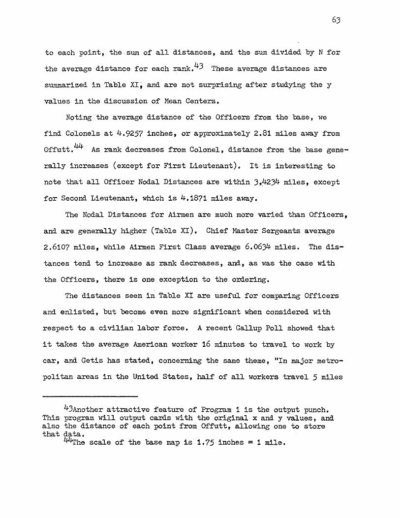
Table X is a summary of the Mean Centers for each rank, from which one can discern some interesting patterns. The x mean for Airmen, for example, begins with the rank of Airman (27,6638), proceeds to Airman First Class (27.865*0, and to Sergeant (27*7625). If the value for Airman First Class was only slightly lower, all of the x means would be perfectly ordered, from the lowest rank (and lowest mean) to the highest rank (and highest mean). The exception appears insignificant, and one can generalize by stating that as rank increases, the mean point of each rank moves eastward, or closer to the base (up the abscissa), since the assigned x value for Offutt is 30*2 (explanation to come in discussion of Nodal Distance).
The y means for Airmen as shown in Table X are almost as perfectly ordered as the x means, but the progression is inverted, that is, as rank increases, the value of the y mean decreases (down the ordinal scale since Offutt•s y = 1.3). This simply illustrates the fact that the lower ranks tend to live farther from the base, as will be more clearly seen in the discussion of Nodal Distance. Airman First Class is again slightly too high in terms of its y value, while Airman is only 0.02 too low, to allow perfect ordering of the y means.
The x means for Officers show consistent values, as their range is only 1.669^, while the range of the Airmen x means is 2.122k (Table X).
M aii programs were written by Mr. Lee C, Bushj Department of Geography, University of Nebraska at Omaha, in collaboration with the author.

58
Program is Mean Center and Nodal Distance
DIMENSION X(500),Y(500),D(500)ASX=0ASY=0AD=0IFIN=0IC0UNT=0READ 100, I0BS,X0,Y0,IR
100 FORMAT(15 f2F5.1115)1 IF(lOBS-(lCOUNT+500))3,3,22 IFIN=500
C-0 TO 43 IFIN=IOBS-ICOUNT4 DO 10 I=1,IFIN
READ 101,X(l),Y(l)101 FORMAT(5X,2F5.15
ASX=ASX+X(I)ASY=ASY+Y(I)D(l)=SQRT(((x(l)-X0)*«2)+((Y(l)-Y0)**2)+0,00001)ad=ad+d (i )
10 CONTINUEIF( 500-IC0UNT) 12,12,11
11 PRINT 200200 FORMAT(1H1,$ MEAN CENTER NODAL DIST PR0GRAM$)
PRINT 201,IR201 F0RMAT(1X,$RANK = $,I5,/,1X,$0BS X Y D 0FFUTT$)12 DO 50 J=1,IFIN
JCOUNT=J+ICOUNTPRINT 102,JC0UNT,X(j),Y(j),D(j)
102 F0RMAT(IX,15,3^5 .1)50 CONTINUE
TYPE 500500 FORMAT(lX,$PREPARE CARD PUNCH$)
PAUSEDO 60 K=1,IFIN KC OUNT=K+IC OUNTPUNCH 103,XC0UNT,X(k ),Y(k ),D(k )
103 FORMAT(15,3x5 .1)60 CONTINUE
IC OUNT=ICOUNT+500if(iobs-icount) 14,13,15
15 type 501501 FORMAT( IX, $ PL ACE NEXT GROUP OF DATA CARDS IN READER$)
GO TO 113 PRINT 104
104 F0RMAT(1X,$ERR0R AD 13$)14 AMX=ASX/(I0BS*1.0)
AMY=ASY/(I0BS*1.0)ATD=AD/(lOBSn.)

59
Program 1 (cont.)
PRINT 105105 FORMAT(1H1, $X MN GTR Y MN CTR AVE D$)
PRINT 106,AHX,AMY,ATD106 FORMAT( IX ,3F10.4)
STOPEND

60
TABLE X COMPARISON OF MSAN CENTERS
Rank X Mean Y Mean2Lt 27.9600 7.1547ILt 28.8832 5.7215Capt 27.5708 5-4929Maj 27.2830 5.2770LC 28.24-38 5*4895Col 28.9524- 5.1952Amn 27.6638 10.7034A1C 27.8654 11.1484sgt 27.7625 10.7203ssgt 27.9621 9.5060TSgt 28.5910 7.9538KSgt 28.9102 6.7808SMS 29.0814 5.1977CMS 29.7862 5.0672

61
There is, however, no orderly progression.The Officer y mean values are interesting in that they are all
”5” values except Second Lieutenant, and the range is only 1.9918 (enlisted range for y means = 6.0812!). There is a progression of the ordinal scale values beginning at Second Lieutenant, with decreasing numbers throughout. Lieutenant Colonel is the lone exception to the general rule. Again, the lower ranks are farther up the ordinal scale from Offutt.
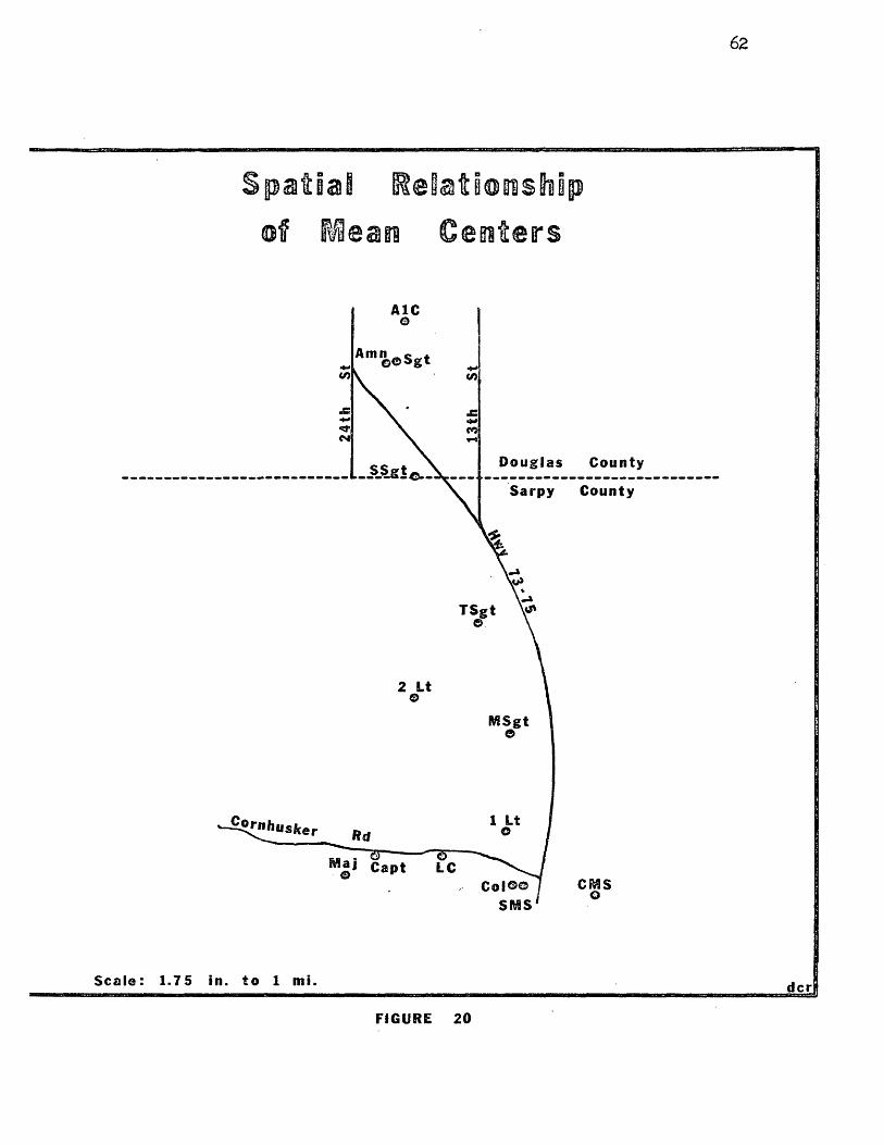
In reviewing the Mean Centers by referring to Figure 20, one can say that they are aligned in a general northwest-southeast direction, with the lower ranks farther north (especially the enlisted means).The three lowest enlisted ranks are well within Douglas County in terms of the mean points, and the fourth is on the county line, while the means for all other ranks are in Sarpy County. The Officer ranks tend to^align themselves along Comhusker Road, with Captain, Major, and Lieutenant Colonel mean points showing the effect of their numbers in Papillion.
Program 1 (page 58) calculated Nodal Distance in addition to Mean Center. Nodal Distance, or the average distance of a distribution from a given point or node (in this case, Offutt), was easily derived since the x and y values for each point were already determined and stored on cards. All that remained was to assign an x and y value to
I 2 2Offutt, and add the c = V a + b formula, or Pythagorean Theorem, to the program.^ The computer then calculated the distance from Offutt
^The values for Offutt, x = 30.2 and y = 1.3» were assigned to the center area of the base, which is approximately the crossing point of the two perpendicular runways (see Figure 2).
62
Spatial Relatiomsiiip ©f Mem Centers
A1C
Douglas County
Sarpy County
TSgt
2 I t
1 Lt
LC
Scale: 1.75 in. to 1 mi. , _
FIGURE 20
63
to each point, the sum of all distances, and the sum divided by N for the average distance for each r a n k . These average distances are summarized in Table XI, and are not surprising after studying the y values in the discussion of Mean Centers.
Noting the average distance of the Officers from the base, we find Colonels at *K9257 inches, or approximately 2.81 miles away from Offutt.^ As rank decreases from Colonel, distance from the base generally increases (except for First Lieutenant). It is interesting to note that all Officer Nodal Distances are within 3*^23^ miles, except for Second Lieutenant, which is 4,1871 miles away.
The Nodal Distances for Airmen are much more varied than Officers, and are generally higher (Table XI), Chief Master Sergeants average 2.6107 miles, while Airmen First Class average 6.0634 miles. The distances tend to increase as rank decreases, and, as was the case with the Officers, there is one exception to the ordering.
The distances seen in Table XI axe useful for comparing Officers and enlisted, but become even more significant when considered with respect to a civilian labor force. A recent Gallup Poll showed that it takes the average American worker 16 minutes to travel to work by cax, and Getis has stated, concerning the same theme, "In major metropolitan areas in the United States, half of all workers travel 5 miles
^3Another attractive feature of Program 1 is the output punch.This program will output cards with the original x and y values, and also the distance of each point from Offutt, allowing one to store that data.
^^he scale of the base map is 1.75 inches = 1 mile.

64
TABLE XIAVERAGE DISTANCE FROM OFFUTT
RankDistance(inches)
Distance(miles)
2Lt 7.3275 4.1871ILt 5.5275 3.1585Capt 5.9911 3.4234Maj 5.9582 3.4046LC 5.6503 3.2287Col 4.9257 2.8146Amn 10.2863 5.8778A1C 10.6110 6.0634Sgt 10.3391 5.9080SSgt 9.3389 5.3365TSgt 7.8116 4.4637MSgt 6.6452 3.7972SMS 5.1032 2.9161CMS 4.5688 2.6107

65
or less to their work."^ Table XI shows that only 4 of the 1^ Air Force ranks average more than 5 miles from Offutt, and all 4 are enlisted ranks. Berry and Horton, in their discussion of the residential location decision, state, "The lower the income, the more constrained will be the choice. Thus, people of lower status live closer to their work than people of higher status."4' While applicable to a civilian populace, this statement is untrue in regard to Offutt8s population.In fact, Table XI indicates that the reverse is true. Further study is needed before a generalization, concerning all military off-base residential distances can be made, thus determining the possible uniqueness of the Offutt case.
Once the Mean Center of a distribution was determined, the Standard Distance Deviation (hereafter SDD) was used to describe the dispersion or spread of the residences of a particular Air Force rank about that mean. SDD is the quadratic average of distances from the Mean Center to each point, or:
/ j: (di - me)2V N
The larger the SDD, the greater the dispersion of residences about the mean point, and vice-versa.
^Arthur Getis, "Residential Location and the Journey From Work," Proceedings of the Association of American Geographers. Volume 1, 1969,p. 5 6.
^°Brian J.L. Berry and Frank E. Horton, Geographic Perspectives on Urban Systems (With Integrated Readings), Englewood Cliffs, N.J.: Prentice-Hall, Inc., 1970, p. 313.
66
Program 2, page 6?, m s written to calculate SDD. The only required inputs are the same x°s and y's used before, and the Mean Center for each rank distribution. Again using the Pythagorean Theorem, the computer calculates the distance from the Mean Center to each point (d^ - me), and, therefore, SDD. Program 2 also utilizes an output punch, and the d (distance) is stored upon cards. These data cards are then input with Program 3 in this series of calculations.
Table XII is a synopsis of the SDD*s according to rank. One can see that the highest SDD is that for Staff Sergeant (7.5947 inches or 4.3398 miles), and there is an ordered decrease in the deviations on both sides of Staff Sergeant. While Staff Sergeant has the greatest spread about the mean, Chief Master Sergeant has the least (4.7639
Inches or 2.7222 miles). The Officer SDD#s are more uniform (values of 5 inches), with only Second Lieutenant not seeiliing to fit with the' others (6.9849 inches).
Program 3» page 699 was written to further refine the dispersion about the mean. This "Concentric Ring" program calculated (using the d from the SDD derivation) the number of Air Force residences in each half-deviation out to four standard deviations (8 "zones"), thus allowing further comparison of one rank with another in terms of spread.^
Three tables have been constructed to analyze the zone distributions.Table XIII summarizes the number of individuals by rank per zone, Table
✓
XIV does the same, but in terms of per cent, and Table XV breaks the
^Program 3 also outputs "Z Score" values. This measure is the actual distance from the Mean Center to each point divided by the SDD.

67
Program 2: Standard Distance Deviation
DIMENSION X(500),Y(500),D(500)SSD=0IFIN=0IC0UNT==0READ 100,IOBS,AMX,AMY,IR
100 F0RMAT(l5,2F10.4,I5)1 IF(IOBS-(ICOUNT+500))3,3122 IFIN=500
GO TO 43 IFIN=IOBS-ICOUNT4 DO 10 I=1,IFIN
READ 101,X(l),Y(l)101 FORMAT(5X,2F5.1)
X(l)=(X(l)-AMX)y (i )=(y (i )-a m y)D(l)=SQRT((x(l)**2 )+(Y(l)**2 )+0.00001) SSD=SSD+(D(l)**2)
10 CONTINUE IF(i-ICOUNT)12,11,1311 PRINT 300
300 FORMAT(IX,$ERR0R ON 11$)13 PRINT 200,IR
200 FORMAT(1H1,$STD DIST PROG RANK « $,15)PRINT 201
201 F0RMAT(1X,$0BS X Y D$)12 DO 50 J=1,IFIN
JCOUNT=J-fICOUNTPRINT 102,JCOUNT,X(j),Y(j),D(j)
102 FORMAT(IX,15,3F5.1)50 CONTINUE
TYPE 500500 FORMAT (IX, $ PREPARE CARD PUNCH$)
PAUSEDO 60 K=1,IFIN KCOUNT=K+ICOUNTPUNCH 103, KCOUNT,X(K),Y(K),D(K)
103 F0RMAT(I5,3F5.1)60 CONTINUE
ICOUNT=ICOUNT+500 IF(l0BS-IC0UNT)l4,14,15
15 TYPE 501501 FORMAT(IX,$PLACE NEXT GROUP OF DATA CARDS IN READER$)
PAUSEGO TO 1
14 SDD=SQRT(SSD/(IOBS*l.0))PRINT 104,SDD
104 FORMAT(IX,/,IX,$STD DIST DEV = $,1F10.4)STOPEND

68
TABLE XXI STANDARD DISTANCE DEVIATIONS
Rank SDD (inches) SDD (miles)2Lt 6.9849 3.9913 ' ^
}
lLt 5.4694 . 3.1253Capt 5.8993 3.3710Ma 3 5.6953 3.2544 3LG 5 .886 -̂ 3.3636 0}Col 5.24-59 2.9976 &
Ann 6.8129 3.8930 2A1G 6.9675 3.9814 7Sgt 7.2996 4.1712 / 2SSgt 7.594-7 4.3398 HTSgt 7.3109 4.1776MSgt 7.174-8 4.0998 nSMS 5.4475 3.1128 3CMS 4.7639 2.7222 /

Program 3: Concentric Kings
DIMENSION IH(8),D(500)READ 100,IOBS,SDD,IRANK
100 FORMAT(15, IF 10.4,15 )'ICOUNT=0IFIN=0 DO 1 1=1,8i h(i )=o
1 CONTINUE2 IF(IOBS-(ICOUNT+500))3,3,43 IFIN=IOBS-ICOUNT
GO TO 54 IFIN=5005 READ 101, (D(j) , J=1,IFIN)
101 F0RMAT(15X,1F5.1)B=0.5DO 10 K=1,IFINd (k )=(d (k )/s d d)
• IF (D(K)-B) 11,11,1211 IH(l)=IH(l)+l
GO TO 1012 IF(d (k )-(2*B)) 13,13,1413 IH(2)=IH(.2)+1
GO TO 1014 if(d(k)-(3*b)) 15,15,1615 IH(3)=IH(3)+1
GO TO 1016 IF(D(K)-(4*B)) 17,17,1817 IH(4)=IH(4)+1
GO TO 1018 if(d(k)-(5*b)) 19,19,2019 ih(5)=ih(5)+1
GO TO 1020 IF(D(K)-(B*6)) 21,21,2221 IH(6)=IH(6)+1
GO TO 1022 IF(d(kM3*7)) 23,23,2423 IH(7)=IH(7)+1
GO TO 1024 IH(8)=IH(8)+1 10 CONTINUE
PRINT 102102 FORMAT(1H1,$CONCENTRIC RING PROGRAM$,/,IX,$Z SCORES
DO 50 L=1, IFINLCNT=L+ICOUNT PRINT 103, LCNT,D(L)
103 FORMAT(IX,15,1F10.4)50 CONTINUE
ICOUNT=IC0UNT+500

70
Program 3 (cont.)
IF(I0BS-IC0UNT)31,2,2 31 PRINT 104,IRANK104 F0RMAT(IX,$Z0NE DISTRIBUTION FOR RANK $,15)
PRINT 105,(lH(M),M=1,8)105 format(ix,116,717)
PRINT 106106 FORMAT(7X,$ 1 2 3 4 5 6
STOPEND
7 8$)

71
TABLE XIII NUMBER OF EACH RAM! PER ZONE
Rank Zone - 1______2______3______42LtlLtCantRajLCColAmnAiCSgtSSgtTSgtMSgtSMSam
21 . 46 18 6 4 0 090 83 6 23 9 1 2185 241 78 38 10 10 383 254 97 23 6 5 284 44 1 24 4 3 22 6 11 1 2 0 0 1
15 21 20 1 1 0 075 9 6 124 12 4 1 0173 226 292 38 8 0 1168 261 254 67 5 0 054 175 33 14 11 1 244 95 14 12 9 3 034 35 3 9 4 0 125 24 3 1 2 2 0
O O
O O
O vH
OO
OO
OO
O-
H

72
TABLE XIV PERCENTAGE OF EACH RANK PER ZONE
Rank Zone 1 2 . 3 4 5 6 7 8
2Lt 22.10 48.42 18.94 6.31 4.21 0 0 0lLt 42.0 5 38.78 2.80 10.74 4.20 0,46 0.93 0Capt 32.74 42.65 13.80 6.72 1,76 1.76 0.53 0Haj 17.65 54.04 20.63 4.89 1.27 1.06 0.42 0LC 51.85 27.16 0.6l 14.81 2.46 1.85 1.23 0Col 61.90 26.19 2.38 4.76 0 0 2.38 2.38
Arnn 2 5* 86 36.20 34.48 1.72 1.72 0 0 0AiC 24.03 30.76 39.74 3.84 1.28 0.32 0 0Sgt 23.44 30.62 39.56 5.14 1.08 0 0.13 0SSgt 22.25 34.56 33.64 8.87 0.66 0 0 0TSgtMSgt
18.62 60.34 11.37 4.82 3.79 0.34 0,68 024.85 53.67 7.90 6.77 5.08 1.69 0 0
SMS 39.53 40.69 3.48 10.46 4,65 0 1.16 0CMS 43.10 41.37 5.17 1.72 3.44 3.44 0 1.72

73
TABLE XVPERCENTAGE OF EACH RANK PER SDD (2 ZONES)
Rank SDD 1 2 ....... 3 ____ 4Jo 2Lt 70.52 25.25 4.21 04 lit 80.83 13.5** 4.66 0.93-7 Capt 75.39 20.52 3.52 0.53dT 71.69 25.52 2.33 0.42- LC 79.01 15.42 4.31 1.23
Col 88.09 7.14 0 4.76^ Amn 62.06 36.20 1.72 0V A1C 5^.79 43.58 1.60 0-■ Sgt 54.06 44.70 1.08 0.13<-*' SSgt 56.81 42.51 0.66 0' '3 TSgt 78.96 16.19 4.13 0.68/ MSgt 78.52 14.67 6.77 0B SMS 80.22 13.9^ 4.65 1.16/ CMS 84.47 6.89 6.88 1.72

7^
zones up into SDD*s.In reviewing Table XIV, the enlisted figures show that Chief Master
Sergeants have the greatest clustering in the immediate vicinity of the mean (43.10% in Zone l), as was indicated by the very low SDD (Table XII), while Technical Sergeants have the least (only 18.62% in Zone l). The others have slightly over 20% in Zone 1, except for Senior Master Sergeants at 39»53^« The two highest enlisted ranks, then, have the greatest concentration at the center.
The rank of Colonel is very.highly concentrated in Zone 1 (61.90%, Table XIV), while Major is not (17.65%). As was the case with the enlisted, the "middle" ranks have the lowest percentages in Zone 1, and the two highest ranks have the highest percentages. The increases are ordered on both sides of the lowest percentages (Technical Sergeant and Major).
The ranks with the highest percentages in Zone 2 have the lowest in Zone 1. Majors have 5^*0Wo in Zone 2, while Technical Sergeantsplace a high 60,34% there (again, Zone 2 is the outermost f- of thefirst SDD). Also, Colonel had the highest in Zone 1, and is lowest in Zone 2 (for Officers), but Chief Master Sergeant (highest Zone 1 enlisted) is not the lowest Zone 2 enlisted. Colonels, then, show great clustering within 1 SDD from the mean point.
Zone 3 contains a wide range of values for both Officers and Airmen, while Zone 4 is comparatively constant.* Zones 5*6»7* and 8 range only from 0 to 5*08%.
Table XV is a summary of the zones in terms of the appropriateSDD (Zones 1 and 2 = SDD 1, Zones 3 and 4 = SDD 2, etc.). This table’

75
attests to the normality or abnormality of each distribution, as a "normal" distribution should have 68% of the occurrences within i standard deviation, 95% of the values should differ from the mean by less than 2 standard deviations, and 95% of the points should be located
hOwithin 3 deviations. Observing the enlisted values in Table XV, one can note that only the four highest ranks are above 68% for the first SDD, while the others are in the 52-60 range. The Chief Master Sergeants present an interesting example, as 84.47% are within 1 SDD, but only 91.36% are within 2 SDD*s. .The lowest enlisted ranks have the highest 2-SDD totals? Airman - 98.26, Airman First Class - 98.37> Sergeant - 98.76, and Staff Sergeant - 99.32! These ranks had the higher SDD * s (Table XII), possibly explaining the high percentages within the first two SDD*s.
The SDD 1 totals for Officers are all above 70.52%. The highest 2-SDD total is that for Major (97.21%), while the lowest is for First Lieutenant (94.37% )•
Once the mean and the dispersion about that mean became known, a requirement existed for classifying the distribution according to randomness, clustering, or uniformity. For this, the author utilized a parametric Nearest Neighbor Analysis for each rank, and Program 4 (page 76) was developed in response.
The first, second, and third nearest neighbor for each point (or residence) was determined, again using the original x and y coordinates and the already-discussed Pythagorean Theorem. The distances between
^John E. Freund, Modem Elementary Statistics. Englewood Cliffs, N.J.: Prentice-Hall, Inc., i960, p. 92.

76
Program Nearest Neighbor Analysis
DIMENSION X(500),Y(500),D(500),SN(3)DO 300 11=1,3SN(1)=0SN(2)=0sn(3)=oIMIN=0AMIN=0BMAX=1000.READ 100,RANK,IOBS,AREA
100 format( 1F5 .0,115 ,-lP10*1)READ 101,(X(l),Y(l),1=1,IOBS)
101 FORMAT(5X,2F5.l)C SELECT FIRST XY POINT
PRINT 200200 FORMAT(1H1,$P0INT NN DISTANCE$)
1 DO 10 J=l,IOBS2 DO 20 K=l,IOBS
D(k )=SQRT(((X(k )-X(J))**2)+((Y(k )-Y(J))**2)+0.00001)20 CONTINUEC RAISE D(J) TO MAX TO ELIM ZERO D AND SEARCH FOR MIN D
3 D(J)=BMAX IGO=l
29 AMIN=10000.DO 25 L=l,IOBS IF(D(L)-AMIN)22,25,25
22 AMIN=D(l )IMIN=L
25 CONTINUESN(IGO)=SN(IGO)+D(IMIN)d (i m i n)=bmaxIGO=IGO+l IF(IGO-3)29,29,10
10 CONTINUE PRINT 203
203 FORMAT(lX,$CUM OF MINIMUM NEIGHBORS$,/,1X,$1ST$,7X,$2ND$,7X,$3RD$) PRINT 2O^,SN(l),SN(2),SN(30
2C& F0RMAT(3F10.2)SNfl)=SN(l ) / (IOBS*l.)SN(2)=SN(2)/(IOBS*l.)SN(3)=SN(3)/(IOBS*l.)H=1.07^6/(SQRT(l0BS/AREA))R=0.5000/(SQRT(IOBS/AREA))RR=0.750/CSQRT(IOBS/AREA))RRR=0.9375/(SQRT(IOBS/AREA))C=0.1TI=(SN(1)+SN(2)+SN(3))/(r+rr+r rr)TDH=SQRT( ( ( SN( 1)-H) **2 W ( SN( 2 )-H ) *^2 )+( ( SN( 3 ) ~H) **2 ) )TDR=SQRT(((SN(1)-R)**2)+((SN(2)~RR)**2)+((SN(3)~RRR)**2))

77
Program 4 (cont.)
TDC=SQRT( ( ( SN( 1 )■-C )**2 )+( ( SN(2 )■-C )**2 )+( ( SN( 3)-C ) **2 ) )PRINT 109,RANK
109 FORMAT(1H1,$NEAREST NEIGHBOR PROGRAM, RANK$,1F5.0)PRINT 110, SN(l),SN(2)fSN(3)
110 FORMAT(IX,$MEAN DISTANCES FOR 1 2 3$,/,24X,3F7.l)PRINT 120
120 FORMAT(1X,$EXPEGTED INDEXES$)PRINT 121,H,H,H
121 FORMAT(IX,$HEXAGON$,18X,1F6.1,IX,1F6.1,IX,1F6.1)PRINT 122,R,RR,RRR
122 FORMAT(IX,$RANDOM$,19X,1F6.1,IX,1F6.1,IX,1F6.l)PRINT 123,C,C,C
123 FORMAT(IX,$CLUSTER$,18X,1F6.1,IX,1F6.1,IX,1F6.1)PRINT 124,TI
124 FORMAT(IX,$TOTAL RANDOMNESS INDEX = $,1F10.5)PRINT 125,TDH
125 FORMAT(lX,$HEX DEV = $,4X,1F10.5)PRINT 126,TDR
126 FORMAT(IX,$RANDOM DEV = $,1X,1F10.5)PRINT 127,TDC
127 FORMAT(IX,$CLUSTER DEV = $,1F10.5)300 CONTINUE
STOPEND

78
nearest neighbors were printed-out, and retained. All distances for first nearest neighbors were summed, and divided by N to determine a mean distance. The same was done for second and third nearest neigh^ bors. Next, mean density (m) was computed.
NB = A
whereN = the number of points A = area
The area used was that within the margins of the original base map (before reduction), 1^35•8 square inches.
After m became known, the expected indices or expected mean distances for first, second, and third nearest neighbors for hexagonal (uniform), random, and clustered were calculated using the following formulae:^
5 JL0246H m
5Rl m
5R2 m
5 , 0,9325. R3~ m
^Numerator values provided by Mr. Charles R. Gildersleeve, Assistant Professor of Geography, University of Nebraska at Omaha, in his course, Geography Concepts (502): Quantitative Methods.

79
D̂ , = a constant, 0.1
wheress mean expected under a hexagonal pattern= hypothetical mean random for first nearest neighbor (^^2= second
nearest neighbor, etc.)= ideal expected under a clustered distribution, which is zero, but a minimum value of 0.1 was assigned.
The "Randomness Index" was computed by comparing the actual mean distances to the expected. The formulae are
t> _ dnni Ri “ ----5 -nnl
whereR^ = Randomness Index for first nearest neighbors
d ^ ^ = actual mean for first nearest neighbors Dnn ̂= expected index for first nearest neighbors
and
-p _ ̂ nn22 " Z---
®nn2
R- = d°n3
°nn3
^The Randomness Index calculation was not a part of Program and computations were done manually.

80
Program ^ also calculated the "Total Randomness Index," which is the sum of the actual means divided by the sum of the expected values, or:
£ dT T
The final step in the Nearest Neighbor Analysis was to calculate "Total Deviation" (of actual mean distances from hexagonal, random, and clustered) using:
TD = £ (d - D)2
The smallest deviation indicates that the distribution is closest to either hexagonal, random, or clustered. If the smallest deviation is from random, for example, then the distribution is random, etc.
Noting Table XVI, one can first compare the actual mean distances for first, second, and third nearest neighbors for each rank. In both cases, Officer and Airmen, the lowest and highest rank have the greatest mean distances. This can, it appears, be simply explained by the fact that these four ranks have fewer total occurrences (see mapped totals, Tables III and VI) than the others, and since mean distance is the sum of all distances for first nearest neighbor divided by N (and the same for second and third), the means should be higher if the N is lower. This notion receives some support from the actual mean distances for Captains, Majors, Sergeants, and Staff Sergeants. These, ranks had the greatest number of observations (and greatest density), and, therefore, the lowest mean distances.

81
TABLE XVIMEAN DISTANCES: ACTUAL VS. EXPECTED*
• Actual Expected Expected Exn. RandomnessMean Hexagonal Random ci. Index
Rank NN-1 2 3 1 2 3 1 2 3 All 1 2 32Lt 0.5 0.9 l.i 4.2 4.2 4.2 1.9 2.9 3.6 0.1 .26 .31 .31^lLt 0.3 0,4 0.5 2.8 2.8 2.8 1.3 1.9 2.4 0.1 .23 .21 .21Ca.pt 0.1 0.3 0.4 1.7 1.7 1.7 0.8 1.2 1.5 0.1 .13 .25 .27Maj 0.1 0.2 0.3 1.9 1.9 1.9 0.9 1.3 1.6 0.1 .11 .15 .19LC 0.4 0.5 0.7 3.2 3.2 3.2 1.5 2.2 2.8 0.1 .27 .23 .25Col 0.7 1.2 1.6 6.3 6.3 6.3 2.9 4.4 5.5 0.1 .24 .27 .29Ann 1.0 1.3 1.6 5.3 5.3 5*3 2.5 3.7 4.7 0.1 .40 .35 .34 /A1C 0.3 0.5 0.6 2.3 2.3 2.3 1.1 1.6 2.0 0.1 .27 .31 .30Sgt. 0.2 0.3 0.4 1.5 1.5 1.5 0.7 1.0 1.3 0.1 .29 .30 .31SSgt 0.2 0.3 0.3 1.5 1.5 1.5 0.7 1.0 1.3 0.1 .29 .30 .23TSgt 0.3 0.5. 0.6 2.4 2.4 2.4 1.1 1.7 2.1 .0.1 .27 .29 .29MSgt 0.4 0.6 0.9 3.1 3.1 3.1 1.4 2.1 2.7 0.1 .29 .29 .33SMS 0.5 0.9 1.2 4.4 4.4 4.4 2.0 3.1 3.8 0.1 .25 .29 .31CMS 0.7 1.1 1.4 5.3 5.3 5.3 2.5 3.7 ^.7 0.1 .28 .30 .30
-̂ Distances, expressed in inches.

82
The actual mean distances in Table XVI can he compared to the expected means for a hexagonal, random, or clustered distribution.In all cases, the actual means are well below the expected for hexagonal, as they are in the case of the random. The actual means are closer to that expected in a clustered distribution, suggesting that the rank distributions tend to be clustered, but the Total Deviations must be analyzed before a final decision can be made.
The Randomness Index for first, second, and third nearest neighbors for each rank is also seen in Table XVI. This index is, as was previously mentioned, the ratio of the mean of the observations to what is expected for randomness. If the ratio is i, then the distribution is random. If it is greater than 1, it tends toward hexagonality, while less than 1 indicates a tendency toward clustering. All of the Randomness Indices in Table XVI are well below 1 (in fact, all are less than 0.5)» once again indicating clusterings.
Total Randomness Index, shown in Table XVII, is merely a composite Randomness Index (sum of actuals divided by sum of expected). These indices for all ranks are also very low, and all are less than 0.^.
The Total Deviations from each distributional type, hexagonal, random, and clustered, were calculated, and are summarized in Table XVII. The deviation from perfectly clustered is smallest in the case of all ranks. Therefore, it appears that the distribution of each rank in the Omaha urbanized area can only be classified as clustered.
The final quantitative method used in analyzing the data was abasic Regression Analysis-. This technique allows one to visualize
</the relationship between x and y, or the general alignment of the

83
TABLE XVIITOTAL RANDOMNESS INDICES AMD TOTAL DEVIATIONS
Total Deviation Deviation DeviationRandomness from from from
Bank Index Hexagonal Random Clustered2Lt 0.29826 5-78925 3.52711 1.36845 ■ILt 0.20385 4.15798 2.67902 0,52426Capt 0.22714 2.51496 1.59151 0.32670Maj 0.17867 2.86147 1.86057 0.25389LC 0.23731 4.65350 2.95569 0.74856Col 0.28067 8.83184 5.44429 1.99833Amn 0.36297 6.99437 4 .15030 2.15544A1C 0.29954 3.18999 1.94610 0.68061Sgt 0.26389 2.13595 1.32913 0.32416SSgt 0.25653 2.12360 1.32999 O .30058TSgt 0.29813 3.31058 2.02930 0.69815MSgt 0.30981 4.20604 2,52928 1.02402SMS 0.28831 6.13417 3.76177 1.39097CMS 0.29590 7.41391 4 .56220 1.74074

Ok
distribution in terms of a regression line, where:
y = a + bx
andb = the slope of the line, or alignment (as used here),
which is the
covariance of x and y variance of x
Program 5 (page 85) was used in calculating b, or the "Least Squares Line. ”51
The "Least Squares Line" was utilized by the author in perhaps a unique way, that is, only to describe the general alignment of the distributions. Since the y axis was placed in a north-south position, and the abscissa is, of course, perpendicular (or east-west), then b gives one the general geographical alignment of each distribution.
Table XVIII contains the slope values for each rank. The most apparent feature of the table is that all of the b values are negatives, indicating that all rank distributions are aligned in a northwest- southeast direction, which is perhaps obvious upon inspection of Figures 5 through 18. The table, though, gives one the degree of slope for each rank; the higher the b, the steeper the slope (more north-south). Table XVIII also contains the a°s (y-intersects) for reference.
^Program 5 will also calculate R (Coefficient of Regression) and Standard Error, as well as list the residuals from regression, but these measures were not considered important to this study.

100
101
102501
103
104
2
105
106
1073200
85
Program 5s Regression Analysis
DIMENSION Y(500),X(500)COMMON SUBRT PRINT 100FORMAT(1H1,IX,$REGRESSION-RESIDUAL PROGRAM^)DO 200 111=1,3 XY=0READ 101, IOBS FORMAT(14)DO 50 1=1,IOBS READ 102,Y(I),X(I)FORMAT(5X,2F5.1)CONTINUECALL AM(Y,YM,YSD,SYY,IOBS)PRINT 103,YM,YSDFORMAT(IX,$Y MEAN = $,Fl4.6,$ STD DEV = $,Fl4.8)CALL AM(X,XM,X3D,SXX,I0BS)PRINT 104,XM,XSDFORMAT(IX,$ X MEAN = $,Fl4.6,$ STD DEV = $,Fl4.8)DO 2 K=1,I0BSxy=xy+((y (k )-y m )*(x (k )-x m ))CONTINUER=XY/(SQRT(SXX*SYY))B=XY/SXXa=y m-(b*x m )SE=SQRT((((IOBS*l.)-l.)/((lOBS*l.)-2.))*(YSD**2)*(1.-(R**2))) PRINT 105,R,A,B,SEFORMAT(IX,$R= $,F7.4,$ A = $,F12.4,$ B= $,F12.4,$ STE = $,F10.4) PRINT 106FORMAT(IX,$NBR$,6X,$Y$,6X,$YEST$,5X,$X$,?X,$RES$,4X,$S RES$)DO 3 L=l,IOBS EY=A+(B*X(L))res=y (l )-eySRES=RES/SEPRINT 107,L,Y(L),EY,X(L),RES,SRES F0RMAT(1X,I4,2X,4F11.3,F11.5)CONTINUECONTINUESTOPEND

86
TABLE XVIII REGRESSION ANALYSIS
Rank a b2Lt 30.1983 -0.3128lLt 31.^938 -O.4563Capt .30.7039 -0.5704Maj 30.1952 -0.5519LC 31.8933 -0.6648*Col 36.7668 -1.5042Amn 32.24-75 -0.4282AiC 31.1880 -0.2980Sgt 31.1630 -0.3183SSgt 30.3345 -0.2496TSgt 30.7566 -0.2723MSgt 31.3001 -O.3525SMS 31.7635 -0.5160CMS 31.6580 -0.3694
, *The values for Colonel are unrealistic, and could have "been caused by the low number of total occurrences (only 42) in conjunction with the N-l (i degree of freedom) used in calculating a*

87
BEHAVIOR AND PROCESS
Decision-Making
"Spatial behavior, exactly as any other behavior, is determined by preferences only."-^ The study of preferences, or decision-making, has been recognized by geographers, and some have even attempted to build spatial choice models in an effort to predict spatial behavior in a system.<53 it is conceivable, and would certainly be interesting, to attempt a model for Offutt*s military population in terms of their residential choices, but such work is beyond the scope of this paper.There are, however, several factors that must be considered which modify the idealized preference, since Offutt and the Omaha area appear unique in some ways.
When the Air Force member begins his tour of duty at Offutt, he usually finds that the housing situation is somewhat difficult. If he is a single Airman or Officer, there is no real problem as barracks space is generally available, should that be desired.^4 The married serviceman, though, often faces difficulty since only Staff Sergeants or higher, and Captains and above are eligible for government family housing, but adequate rank by no means insures space since there is a critical shortage (see page 6). As a result, large numbers of personnel
-^Gerard Rushton, "Analysis of Spatial Behavior by Revealed Space Preference," Annals of the Association of American Geographers. Volume 59» Number 2, June, 19&9* p. 400.
53see, in addition to Rushton, Donald Demko and Ronald Briggs, "A Model of Spatial Choice and Related Operational Considerations," Proceedings of the Association of American Geographers. Volume 3* 1971* pp. ^9-52.
5^Single Airmen (E-l, E-2, and E-3) must live on base (see footnote 8).

88
face the decision as to proper housing within the civilian- community.The military situation appears to cause some peculiarity in re
gard to factors influencing the decision. One such unique factor is "sponsorship." A career serviceman experiences many "Permanent Changes of Station" (PCS) during his years in uniform. He is usually alerted as to his pending move several months in advance, and a sponsor, often a man of equal rank, is assigned to him at the new base. The duties of the sponsor include writing to the man, and generally providing information about the new base, while making some advance preparation for the incoming person's family. In terms of off-base housing, the residential locale of the sponsor could thus influence the decision of the new assignee.
Availability of housing plays an important role in the Offutt area. This shortage is a common complaint, and is largely part of the impact of such a large base upon the civilian communities around it.
Another factor in the military residential decision is organizational assignment. Many of Offutt's personnel spend a few days in one of the area's motels while they begin work, and continue to search for adequate shelter. Often, the new assignee will be influenced by a coworker in the new squadron. The question usually is, "Have you found housing yet?" If the answer is no, the reply is often, "I know of a vacant apartment in our building," or, "There is a house for rent in our block." This process, which also causes-persons established in the area to move, is very read, and would be an interesting correlative study (squadron assignment compared to residential location). But these factors, especially the first, appear somewhat unique to the
89
military, and there are other, more important considerations.Brian Berry, with reference to a civilian urban group, notes:
The principal determinants of their choice of housing are three in number: the price ofthe dwelling unit (either rent or purchase); the type of residence; and its location, both in terms of neighborhood environment and in relation to place of work. These determinants have parallels in the attributes of the individual making the choice of housing; the amount he is prepared to pay for housing, which depends on his income; the housing he needs, which depends on his marital status and family size (i.e., his stage in the life cycle); his life style preferences, which will affect the type of. neighbor he wants; and finally, where he works and how close to the job he must live.-5 ̂
The decision-making factors suggested by Berry appear to operate similarly in the military instance, and warrant some elaboration.
The first, and probably most obvious, consideration in the search for housing is cost, which establishes the limitations as to the type of housing selected, as well as the general social class or environment of the neighborhood in which a particular household unit is lo-' cated. An Airman (E-2), for example, cannot afford to buy, or even rent in many cases, a house according to his rate of pay (see Table XIX). He, therefore, becomes restricted to an apartment (usually one of low cost) or a rented trailer. Conversely, a high-ranking Non-Commisioned Officer (E-8 or E-9) or an Officer (Captain or higher)
/
can easily afford a high-class apartment, a rented house, and even to buy a house. Thus, some of the patterns evident in Table XX begin to be more comprehensible.
-̂ -̂ Berry and Horton, or. cit.. p. 311.

90
Source:
TABLE XIXy
OFFICER AND AIRMAN PAY SCALES
MONTHLY RATES OF PAY OF COMMISSIONED OFFICERSYEARS OF SERVICE
Pay Grade Under 2 Over 2 Over 3 Over 4 Over 6 Over 8 Over 100-10 ..... 2111.40 2185.80 2185.80 2185.80 2185.80 2269.50 2269.500-9 ...... 1871.40 1920.60 1961.70 1961.70 1961.70 2011.20 2011.200-8 ...... 1695.00 1745.70 1787.40 1787.40 1787.40 1920.60 1920.600-7 ...... 1408.20 1504.20 1504.20 1504.20 1571.10 1571.10 1662.600-6 ...... 1043.70 1147.20 1221.90 1221.90 1221.90 1221.90 1221.900-5 ...... 834.60 980.70 1047.90 1047.90 1047.90 1047.90 1080.300-4 .... 704.10 856.50 914.40 914.40 930.60 972.30 1038.300-3* ..... 654.30 731.10 781.20 864.90 906.00 938.70 989.100-2* ..... 524.40 622.80 748.20 773.10 789.30 789.30 789.300-1* ..... 450.60 499.20 622.80 622.80 622.80 622.80 622.80
YEAftS OF SERVICE
Pay Grade Over 12 Over 14 Over 16 Over 18 Over 20 Over 22 Over 260-10 ..... 2443.50 2443.50 2618.40 2618.40 2793.30 2793.30 2967.600-9 ...... 2094.60 2094.60 2269.50 2269.50 2443.50 2443.50 2618.400-8 ;..... 2011.20 2011.20 2094.60 2185.80 2269.50 2361.00 2361.000-7 ...... 1662.60 1745.70 1920.60 2052.60 2052.60 2052.60 2052.600-6 ...... 1221.90 1263.30 1463.10 1537.80 1571.10 1662.60 1803.300-5 ...... 1137.90 1213.80 1304.70 1379.70 1421.10 1471.20 1471.200-4 ...... 1097.10 1147.20 1197.00 1230.30 1230.30 1230.30 1230.300-3* ..... 1038.30 1063.80 1063.80 1063.80 1063.80 1063.80 1063.800-2* ..... 789.30 789.30 789.30 789.30 789.30 789.30 789.30O-l* ... 622,80 622.80 622.80 622.80 622.80 622.80 622.80*Does not apply to officers who have been credited with aver 4 years' active service as enlisted members.
M O N T H L Y RATES OF PAYYEARS OF SERVICE
Pay Grade Under 2 Over 2 Over 3 Over 4 Over 6 Over 8 Over 10 Over 12E-9........ $701.40 $717.60E-8........ $588.60 605.10 621.00E-7........ $369.90 $443.40 $459.90 $476.10 $492.30 507.90 524.10 540.90E-6........ 318.90 387.30 403.20 419.70 435.90 451.80 468.30 492.30E-5........ 275.40 339.30 355.50 371.70 395.40 411.60 427.80 443.40E-4........ 231.60 290.10 306.60 330.60 347.10E-3........ 167.70 233.70 249.90 266.40E-*>........ 138.30 193.50E-1........E-1 Under
4 months .133.20124.50
177.00 __
YEARS OF SERVICEPay Grade Over 1 4 Over 16 Over 18 Over 20 Over 22 Over 24 Over 26E-9........ $734,10 $750.30 $767.10 $782.10 $823.50 $823.50 $903.60E-8........ 637.50 653.70 669.30 685.80 726.30 726.30 807.00E-7........ 564.90 580.80 597.00 605.10 645.60 645,60 726,30E-6........ 507.90 524.10 532.50E-5................ 451.80E-4......................E-3......................E-2......................E-1......................
"Airman9s Pay Guide," January 1, 1970, and "Officer’s Pay Guide," January 1, 1971#
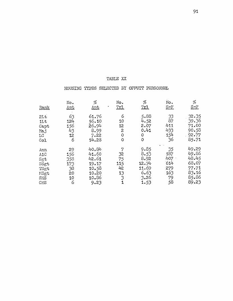
TABLE XXHOUSING TYPES SELECTED BY OFFUTT PERSONNEL
No. % No. of/O No. <Rank Ant Ant Trl Trl S-F S-F2Lt 63 61.76 6 5.88 33 32.35ILt 124 56.10 10 4.52 87 39.36Capt 156 26.94 12 2.07 411 71.00Maj 43 8.99 2 0.41 433 90.53LC 12 7.22 0 0 154 . 92.77Col 6 14.28 0 0 36 85.71
Amn 29 40.84 7 9.85 35 49.29A1C 156 4-1.60 32 8.53 187 11-9.86Sgt 358 42.61 75 8.92 407 ' 48 .45SSgt 173 19.17 115 12.74 614 68.0?TSgt 38 10.58 42 11.69 279 77.71USgt 20 10.20 13 6.63 163 83.16SMS 10 10.86 3 3.26 79 85.86CMS 6 9.23 1 1.53 58 89.23

92
The rank as a predictive factor in housing type and social class of the unit is not, of course, valid in all instances. Many'of Offutt#s lower-grade enlisted personnel have working wives, and many hold part- time civilian jobs, thus widening their range of choice of housing.Also, the accustomed life style may play a deterrent role in a "rank- predictive analysis," but the method probably holds true in most cases, as is shown in Table XX.
As Berry suggests, one®s stage in the life cycle is an important factor in the type of housing seLected. Airmen (E-2), Airmen First Glass, Sergeants, some Staff Sergeants, Second Lieutenants, First Lieutenants, and some Captains tend to be younger, with small families, if any at all. An apartment is often adequate, and Table XX shows that these ranks have the highest percentages in apartments. The persons of other ranks are usually older, with larger families and older children that require more room, thus explaining the higher percentages in single-family houses for these higher ranks.
Looking at Table XX more closely, one can note that the percentage of Officers living in apartments and trailers generally increases as rank decreases, while the percentage in houses increases as rank increases. Note also that the rank of Colonel does not exactly fit the progression. This is probably because Colonels are usually the oldest of all the ranks studied, and most have already raised a family that has since left home, so they tend to move back to the apartments, as less room is needed.
The enlisted statistics found in Table XX are also worthy of some discussion. The ranks of Chief Master Sergeant, Senior Master Sergeant,
93
Master Sergeant, and Technical Sergeant all have about 10% in apartments , while Staff Sergeant has 19.17%. The lowest three ranks have slightly over 40% in apartments, and, as was previously stated, the percentage in apartments tends to increase as rank decreases.56 Regarding trailers, the lowest five enlisted ranks range from 8.53% to 12.74%. Very few individuals of higher ranks live in trailers. There is a general increase in single-family percentages as rank increases, as was the case with Officers.
Berry*s final point (page 89.) > that of proximity to work, was discussed earlier.. It was determined that distances generally increase as rank decreases, and that the average distance traveled daily is usually less than 5 miles (10 of the 14 ranks). Joumey-to-work is an important factor in residential location decision, as the previous figures indicate.
Q.uestionaire Results
Why do the patterns that have been illustrated in Figures 5 through 18 exist, and what do the military individuals, themselves, consider to be the most important factors in residential location decision? Why, then, does the military man settle where he has? In an attempt to
56A11 of the statistics for Table XX were derived from the individual's stated address. If an apartment number was listed followingthe street address, that individual was added, of course, to the apartment statistics. The author, however, is inclined to believe that the apartment statistics for the three lowest enlisted ranks are lower than they should be, and the single-family figures are too high (especially for Airman and Airman First Class). This error could arise due to omission of an apartment number when listing one's address, and was possibly done frequently enough to cause these somewhat unrealistic figures.

94
answer these questions, the author interviewed 186 Offutt servicemen by means of the questionaire shown as Figure 21. The questionaires were distributed by hand on a random basis. They comprise, however, only a 4.14% sample of the total 4,488 individuals that reside off-base, but the answers given serve as a good foundation for judgement as to the decision process.
The reasons listed on the questionaire by the author were patterned, to some degree, after those suggested by Cole.57 Space was left for the respondent to cite other reasons for residential choice that were not listed by the writer. The individual had only to state his rank, check what type of housing he maintains, what'community he lives within, and why he chose his residence. He was told to cite as many reasons as were applicable. The final question pertained to base housing, and was included only to solicit opinion on that topic.
Table XXI is an evaluation of the responses in terms of rank. The most frequently cited reason for residential location was "clean and quiet neighborhood” (76), followed by "closeness to Offutt" (58), "nearness to good roads allowing easy access to the base" (48), and "it was the only available location at the time” (42). More Airmen responded than Officers (137 to 49)» but note that all but one of the "all I could afford" responses are by those of the enlisted ranks.
Table XXII summarizes these responses in terms of percentages."Glean and quiet neighborhood" accounted for 21.2% of all 358 responses, and, although this was the most important consideration, there appeared
5?Cole, OT3. cit. t p. 12.

95
SAMPLE QUESTIONAIRE
Rank
Please Check the A-p-pronriate Statements
I reside off-base, and live in a(n); apartment rented house house which I own myself trailer other (please specify)__
I live within the city of: _Omaha Bellevue Papillion Plattsmouth other (please specify)
I chose my residential location because: I wanted to be as close to Offutt as possible. I wanted to locate close to a school for my children. I like to be far from the base when Ifm off-duty. _it is a clean and quiet neighborhood. it is out of the city. it was all I could afford. it was the only available location at the time. it was of easy access to good roads leading to the base. a friend of mine lived -there. I plan to retire in this area. it is near my part-time job. it was the only place I could live, as I feel there
is local racial discrimination. . other (please specify)____________________________
If I could, I would. __live on the base in federal housing. not live on the base.
Use the space below for any other comments you may have.FIGURE 21

96
TABLE XXI NUMBER OF RESPONSES BY RANK
Rank *A B G D E F G H I J K L M2Lt 1 0 0 1 0 0 0 0 0 0 0 • 0 1lLt 3 0 0 1 0 1 2 2 0 0 0 0 0Capt 10 6 1 13 1 0 2 9 1 0 0 0 3Maj 5 k 1 8 1 0 1 2 2 0 1 0 kLG 2 J> 0 1 0 0 0 1 0 1 0 0 2Col 1 0 0 1 0 0 0 0 0 0 0 0 0
+SA 0 0 0 0 0 0 1 0 0 0 0 0 1Amn 0 ' 0 0 0 0 1 0 1 0 0 0 0 0A1G 2 0 5 6 1 5 k 3 0 0 1 0 0Sgt 12 1 k 13 k 10 10 10 k 0 3 0 6SSgt 5 9 22 5 5 13 Ik 5 0 0 0 6TSgt 6 3 0 5 2 3 7 3. 0 0 0 0 kMSgt 1 2 1 2 0 2 l 2 1 0 0 0 1SMS 0 0 0 2 0 0 l 0 0 1 0 0 0CMS 1 0 0 1 0 0 0 1 0 0 0 0 0
*Key to ResponsesA - as close to Offutt as possible B - close to a school for my children G - like to be far from the base when I*m off-duty D - clean and quiet neighborhoodE - out of the cityF - all I could affordG - the only available location at the timeH - of easy access to good roads leading to the base I - a friend of mine lived there J - plan to retire in this area K - near my part-time jobL - only place I could live; local racial discriminationM - other; see Table XXIII
+OSI Special Agent

97
TABLE XXIIREASONS GIVEN FOR RESIDENTIAL LOCATION CHOICE
Reason % of Total Responses*-- Clean and quiet neighborhood. ...... 21.2_Close to Offutt. ....... 16.2-Near good roads leading to base................ 13*4Only available location. ..... 11.7
-Other. ........ 7*3- All I could afford ...... 7.5-Close to schools ..... 6.7- Like to be far from the b a s e 5*9Out of the city ......... 3*9A friend lived t h e r e 3*6Near part-time job, .... 1.4Plan to retire in this area.................... 0.6Racial Discrimination. ...... •••• 0
*There were 353 total responses, for an average of 1.92 responses per person.
»

98
to be much thought given to the joumey-to-work, as the "close to Offutt" response and "good access roads" choice totaled 16.2$ and 13.4$ respectively. "Only thing available" was fourth with 11.?$, and "other" was fifth at 7.8$. As noted, the "other" responses are elaborated upon in Table XXIII.
The respondents appeared to constitute a fairly good cross-section of Offutt servicemen in terms of the community where they reside, types of housing selected, and rank. Table XXIV summarizes the community-of- origin figures, showing 46,2$ coming from Bellevue, 32.3$ from Omaha,v
5*9$ from Plattsmouth, and 5*4$ from Papillion (compare with Table IX). Other communities were also represented. Housing types of the respondents by rank are listed in Table XXV, and persons from all types are represented.
The final entry on the questionaire concerned base housing. It is interesting to note that 144 said that they would not want base housing even if it was available, and only 37 stated that they would accept it (5 did not respond to this question).

TABLE XXIIIREASONS CITED UNDER "OTHER" RESPONSE
Reason No.Close to wife * s job........................ 4Base housing u n a v a i l a b l e 3Close to the university... 3Base housing inadequate.................... 2Near church. ...... 2Bought a trailer in that location.«....•••• 2Good quality schools ...... 1*x'?lan to stay in area when separated. •••••.. 1No rioting or burning...................... iArea is free of dogs and kids.............. 1Near stores.....*.... .................. . 1Area is good for night l i f e 1 Needed a large h o u s e i Liked the yard and t r e e s 1Personal reasons •....... 1Scenic drive to work. ........ 1Close enough to ride bike to work.......... iNo special r e a s o n . 1
*A "first-term" Airman? not a career serviceman, therefore, not "retirement," but "separation."

100
TABLE XXIVHOME COMMUNITY OF RESPONDENTS
No. % .of Total46.2
60 32.3Plattsmouth. 11 5.9
5 >Sarpy Go. Omaha.......... 2.7
2.71.6
Rt. 3 1 Omaha.............. 1.6Council Bluffs........... 0.5
0.5Douglas Co............... 0.5
*

lOi
TABLE XXV HOUSING TYPES OP RESPONDENTS
. Rank AptRentedHouse
Self-OwnedHouse
2Lt 2 0 1ILt 2 2 1C'apt 1 b 16Maj 2 0 13LG 0 0 3Col 0 0 1SA 0 0 0
Aim 1 1 0A 1C 10 5 0Sgt 2? 4 2SSgt 2^ 11 10TSgt 4 0 8MSgt 1 3 2SMS 0 1 1CHS 0 0 1^Lives with a relative. Response -
Trailer Other Total0 0 31 0 60 0 210 0 150 0 30 0 12 0 20 0 21 0 164 i* 3810 0 552 0 1 ^1 0 ?0 0 20 0 1
“all I can afford."

102
IMPACT OF MILITARY BASES UPON THE SURROUNDING AREA
Population Comparisons
The impact of a large military installation upon the surrounding area is manifest in several ways. One of the more readily-seen changes is in the population growth of the region. Whelan noted in his study of Dover Air Force Base, Delaware, that population increased in minor civil divisions (representative districts) around Dover Air Force Base from 12.2% up to 319*2% over the .1950“i960 decade.58 Pietz also recorded remarkable population growth figures for Craven County, North Carolina, after the Cherry Point Station was built in 1 9 ^ 1 During the 19^0-1950 decade, the population of Craven County increased at a rate of 1,379%, while 1950-1960 saw a 5 ^ increase.^
This great population increase can benefit the economy of an area, but problems often arise from this type of "overnight" growth. The city of Plattsburgh, New York, for instance, thought that an Air Force Base would boost its sagging economy, which it did, but the population spurted from 20,000 to 35,000 almost overnight, and a severe housing shortage was the result,^1 Frownfelter noted that while the economic impact of Fort Wolters on the city of Mineral Wells, Texas, was immense, the great influx of military personnel had other effects, such as dependent children causing school overcrowding.^ Thus, the impact that
-5%reese, op. cit., p. 309*^pPietz, pp. cit., p. 62.Zkid, p. 63.
61"Air Base Goads a Town to Grow," Business Week, July 27, 1957, p» 1^4* 62james 0. Frownfelter, "The Economic Impact of Fort Wolters, Texas,
on the City of Mineral Wells, Texas." Unpublished Research Paper, University of Nebraska at Omaha,* April, 1970*

103
large numbers of people associated with a military installation will have on an area is not to be underestimated.
Offutt Air Force Base has stimulated’ population growth in the Omaha area, and especially in Sarpy County.
In the 1950*s» Sarpy County8s population nearly doubled. In the 19608s, it more than doubled. Preliminary 1970 census figures indicate that during the last 10 years Sarpycs population rose from 31,391 to 65,^30, an increase of 109.2 per Cent. Sarpy now ranks eighth among the 10 fastest growing counties in the nation,
What are the forces behind this burgeoning population growth? The close proximity of Sarpy County to the city of Omaha is certainly a catalyst for growth, as Sarpy serves as a "dormitory” for many Omaha workers. But Offutt appears equally important, and, as Bresette noted, "The population of the county also closely parallels the growth of Offutt...."^4' Bellevue had only 3*800 people in 1950» and today it has 21,500, while LaVista, which did not exist in 1950, now has a population of 4,381.^ Considering all military, civilian, and dependent personnel, the Offutt population exceeds 35*000, making it the third largest "city" in Nebraska. 00 Reference to any of the population maps (Figures 5“18) presented earlier in this thesis certainly lends credence
^3James Bresette, "Omaha and Offutt Spur Sarpy," Omaha World-Herald. Wednesday, September 23* 1970, p. 21.
^Ibid. p. 22.65"SAC Pumps 8Lifeblood8 in Economy," in "SAC and the Community,"
Special Supplement to the South Omaha Sun. Section C, March 18, 1971*P . 12Gy
° John Taylor, "Third City Helps Put Go Into Economy of Metro Area," in "SACt 25 Years on Guard," Special Supplement to the Omaha World- Herald, March 21, 1971* p. 13*

10**
to the notion that military personnel are an integral part of the county, and Offutt surely is an important factor in the physical growth of Sarpy County and its cities.
Economic Impact
The physical growth, or population impact, of a military installation usually is a "boon to the economy of the area. Whelan studied the economic changes through time in Dover, Delaware, and found labor force increases of 325% during the 1950~1960 decade (the base opened in 1952).^ These large increases were in the fields of transportation, communications, and public utilities. Whelan noted, "It is probably in the field of retail trade that the prescience of the Air Force has most significantly affected the trading growth of the Dover area."Retail sales in Dover increased 85.*$ from 19^8 to 195^ (a* period ofbase buildup), and several new shopping centers were built in the early
6q1960#s . In 19^1, the "...Air Base payroll accounted for approximately one third of the total wages in the county....
Pietz stated that the wages of the civilian employees and the marines at Cherry Point, which were more than $60 million in 1 9 are very important to the local e c o n o m y . H e also noted that the adjacent city of Havelock is completely dependent upon the Air Station.^
^Breese, op. cit.. p. 323*° Ibid. p. 327.69ibid, p. 330.7°Ibid, p. 327.71pietz, op. cit.. p. 116.72Ibid, p. 117.

105
Offutt Air Force Base is a very substantial factor in the economy of the Omaha area.
In Fiscal Year 1965, ^he Offutt civilian payroll for 1,300 employees amounted to approximately $11 million while 10,500 officers and enlisted men received over $70 million in paychecks. Coupled with the $36.8 million spent by Offutt for locally purchased material and services, Offutt Air Force Base was directly responsible for bringing over $117.8 million in new funds into the Omaha area from 1 July 6^ to 30 June 65.^
For comparison, consider these figures for Fiscal Year 1970. Offutt®s payroll was $1^3.7 million, with an additional $18.8 million spent on local procurement purchases.7^ Of the $18.8 million, $15.2 million was spent within 50 miles of Offutt, and $6.8 million was paid to small businesses.75 The $1^3*7 million payroll was spent as follows: Food -22.7%9 Housing - 23.5%» Transportation - 1^,2%, Clothing, Recreation, and Education - 22.3^» Taxes, Insurance, and Misc. - V7*3?oP^
While Offutt is important to the economy of the Omaha area in general, it is essential to the city of Bellevue in particular. Young studied the influence of Offutt upon Bellevue, and estimated that base personnel spend $2,33^,875 Per month in Bellevue.77 He investigated
73Henry R. Blair, "The Economic Impact of Offutt Air Force Base on the Douglas-Sarpy County Area," Unpublished Research Paper, University of Omaha, May 2, 1966, p. 3 . See also, John E. Lynch, Local Economic Development After Military Base Closures. New York: Praeger Publishers,1970, p. 315* Lynch lists the Offutt monthly payroll at $6,267,000 for military, and $1,171,000 for the civilian employees.
7^"SAC Pumps •Lifeblood® in Economy," op. cit.. p. 12C.75Ibid.76raylor, op. cit.« p. 13.77Robert W. Young, "Bellevue-Offutt Air Force Base-Bellevue: A
Study of Influence," Unpublished Reseaxch Paper, University of Nebraska at Omaha, January, 1970, p. 7.

106
Bellevue shopping areas, counting cars with Base decals, and found results that range from 40% to 66$> of all cars. Young noted,too, the impact funds, over $3 million, that Bellevue receives each year for federal dependent students.
The overall impact of Offutt is vast, but the economic impact is especially important. Should the base ever close, the area's economy, and especially that of Bellevue, would be severely impaired.

10?
SUMMARY AND CONCLUSIONS
This thesis has examined the off-base residential locations of ^,022 Offutt Air Force Base military personnel, and noted the regularities in the distributions, both in terms of an Officer-Airman di- • chotomy, and by individual rank. The original hypothesis, that military rank is important in residential location, and that there are clusters according to rank, has been illustrated in Figures 5 through 18. The distributions have also shown that the main traffic arteries are a factor in residential location. "Rank-progressions" were noted in terms of community of residence, and predictable patterns have emerged. The role of rank in the selection of housing type was found important. Rank is also a factor in distance traveled daily to work at Offutt, but unlike a civilian populace, those of lower status tend to travel a greater distance. A "commuting zone" for the base was established.The quantitative comparisons revealed a number of regularities in this military population, from the alignment of the Mean Centers to the clustering tendencies. Some reasons for residential decision-making were suggested, and the tremendous impact of Offutt on this area was also•discussed.
It is hoped that this study has shed some light on a subject that has been generally neglected by geographers. While there is much work to be done on the topic of the dispersion of military personnel into a civilian community, this analysis of Offutt Air Force Base has shown that there are many consistent or regular relationships. Interesting complementary studies could include a Nearest Neighbor Analysis in terms

108
of individual communities, a study of percentages of servicemen living in apartment complexes located throughout the Omaha metropolitan area, a correlation analysis of travel-time and military rank, housing types selected with regard to the community that they are located within, and residential location compared to squadron assignment. Many other avenues of inquiry remain open, and this paper may stimulate more new ideas.

109
BIBLIOGRAPHY
"A Chronology of Offutt.Air Force Base." Offutt Air Force Base Publication, 210-1-1, January 1, 1962.
"Air Base Goads a Town to Grow." Business Week, July 27, 1957» pp. jM-150."Airman’s Pay Guide." January 1, 1970, Personal Affairs Office, Offutt
Air Force Base, Nebraska.Alonso, William. Location and Land Use. Cambridge! Harvard University
Press, 1964.Berry, Brian J.L. and Horton, Frank E. Geographic Perspectives on
Urban Systems (With Integrated Readings). Englewood Cliffs, N.J.: Prentice-Hall, Inc., 1970.
Blair, Henry R. "The Economic Impact of Offutt Air Force Base on theDouglas-Sarpy County Area." Unpublished Research Paper, University of Omaha, May 2, 1966.
Boyer, W.R. "Bellevue, Nebraska: Problems of Growth and Expansion."Unpublished Research Paper, University of Nebraska at Omaha, January 8 , 1970.
J Breese, Gerald, et al. The Impact of Large Installations on NearbyAreas. Beverly Hills, California: Sage Publications, Inc., 1965.
Bresette, James. "Omaha and Offutt Spur Sarpy." Omaha World-Herald. Wednesday, September 23» 1970, p. 21.
Carroll, J. Douglas, Jr. "Some Aspects of the Home-Work Relationships of Industrial Workers." Land Economics. Volume 25, Number 4, November, 1949, pp. 414-422.
_______. "The Relation of Homes to Work Places and the Spatial Patternof Cities." Social Forces. Volume 30, March, 1952.
/cole, David B. "Military Residential Patterns in a Civilian Community." Unpublished Research Paper, Presented at the Annual Meeting, Great
„ Plains-Rocky Mountain Division, Association of American Geographers, U.S. Air Force Academy, Colorado Springs, Colorado, October, 1970.
Cole, John P. and King, C.A.M. Quantitative Geography: Techniquesand Theories in Geography. New York: John Wiley and Sons, Ltd.,1969.
Demko, Donald and Briggs, Ronald. "A Model of Spatial Choice and Related Operational Considerations." Proceedings of the Association of American Geographers. Volume 3, 1971, pp. 49“52.

110
Duncan, Otis D. and Duncan, Beverley. "Residential. Distribution andOccupational Stratification." In Hatt, Paxil K. and Reiss, Albert J., Jr. (eds.), Cities and Society. Glencoe, Illinois: The FreePress, 1959•
______. "The Measurement of Intra-City Locational and ResidentialPatterns." Journal of Regional Science. Volume 2, Number 2, i960, PP. 37-54.
Enlisted Master File Listing. Accounting and Finance Office, Offutt Air Force Base, Nebraska, January 7, 1970.
"Fact Book: December, 1970." 3902 Air Base Wing, Offutt Air ForceBase, Nebraska.
Frexind, John E. Modem Elementary Statistics. Englewood Cliffs, N.J.: Prentice-Hall, Inc., i960. ,
Frownfelter, James 0. "The Economic Impact of Fort Wolters, Texas, on the City of Mineral Wells, Texas." Unpublished Research Paper, University of Nebraska at Omaha, April, 1970.
Getis, Arthur. "Residential Location and the Journey From Work."Proceedings of the Association of American Geographers. Volume1, 1969, pp. 55-59.
Hansen, Ronald L. "A Study of Furnished Apartments of Omaha." Unpublished Research Paper, University of Nebraska at Omaha, June, 1970.
Haxt, John Fraser. "Central Tendency in Areal Distributions." • Economic Geography, Volume 30, January, 1954, pp. 48-59•
Johnson, James H. Urban Geography: An Introductory Analysis. NewYork: Pergamon Press, 1967; Esp. Chp. 7? "Residential Suburbs:The Journey to Work."
Kain, John F. "The Journey to Work as a Determinant of ResidentialLocation." Papers and Proceedings of the Regional Science Association. Volume 9, 1962, pp. 137-160.
King, Leslie J. Statistical Analysis in Geography. Englewood Cliffs, N.J.: Prentice-Hall, Inc., 1969.
Knox, Elena Amelia. "A Simulation Model of Urban Residential Location Based Upon the Location of Workplaces." Unpublished Master's Thesis, Rutgers University, 1969.
Liepmann, Kate K. The Journey to Work: Its Significance for Industrialand Community Life. London: Kegan Paul, Trench, Trubner, andCo., Ltd., 1945.

Ill
Loewenstein, Louis K. "The Industry of Employment: A Neglected Factorin the Spatial Distribution of Residences in Urban Areas." American Journal of Economics and Sociology. Volume 2 k, Number 2, April,1965> PP« 157-162.
___________. The Location of Residences and Work Places in Urban Areas.New York: The Scarecrow Press, Inc., 1965.
Lowry, Ira. A Model of Metropolis. Santa Monica, California: TheRand Corporation, 196^.
JLynch, John E. Local Economic Development After Military Base Closures. ̂ New York: Praeger Publishers, 1970.McCormick, B., Pick, C., and McWilliams, R. "Apartment Rents: One
and Two Bedroom Unfurnished (in Omaha)," Unpublished Research Paper, University of Nebraska at Omaha, July, 1970.
"Military Training." Lackland Military Training Center, Lackland Air Force Base, Texas, May, 1966.
x/ Monaghan, Louise K. "Military Bases as Nuclei for Urbanization: WarnerRobins, Georgia." Unpublished Master’s Thesis, University of Tennessee, 1968.
Murphy, Raymond E. The American City: An Urban Geography. New York:McGraw-Hill, Inc., 1966} Esp. Chp. 18: "Urban Residential Patterns."
Officer Information Directory. Headquarters Strategic Air Command and Offutt Air Force Base, Nebraska, August 30, 1969*
Officer Master File Listing. Accounting and Finance Office, Offutt Air Force Base, Nebraska, January 7» 1970.
"Officer’s Pay Guide." January 1, 1971* Personal Affairs Office, Offutt Air Force Base, Nebraska.
"Offutt Air Force Base and SAC Headquarters Base Guide, 1969-1970." Published by Sun Newspapers, Omaha, Nebraska.
^Pietz, Reuel Henry. "The Impact of the Cherry Point Marine Corps Air Station Upon Local Settlement." Unpublished Master’s Thesis,East Carolina College, 196^.
Roster of Enlisted Personnel. Offutt Air Force Base, Nebraska, September, 1969.
Rundquist, Donald C. "The Distribution of Military Personnel Around Offutt Air Force Base, Nebraska." Unpublished Research Paper, University of Nebraska at Omaha, January 8, 1970.

112
Rushton, Gerard. "Analysis of Spatial Behavior by Revealed Space Preference." Annals of the Association of American Geographers. Volume 59> Number 2, June, 19&9> PP« 391-^00.
"SAG Pumps 8Lifeblood® in Economy.” In "SAG and the Community," Special Supplement to the South Omaha Sun, Section G, March 18, 1971* p. 12C.
Sauer, Carl 0. "The Education of a Geographer." In Leighly, John,Land and Life. Berkeley: University of California Press, 1967,pp. 389-^0^.
Schnore, Leo F. The Urban Scene: Human Ecology and Demography. New Yorks The Free Press, 1985? Esp, Chp. 19s "The Separation of Home and Works A Problem for Human Ecology."
Taaffe, Edward J. Geography. Englewood Cliffs, N.J.: Prentice-Hall,Inc., 1970.
Taylor, John. "Third City Helps Put Go Into Economy of Metro Area."In "SAG: 25 Years on Guard," Special Supplement to the Omaha World-Herald. March 21, 1971.
^/wheeler, James 0. "Residential Location by Occupational Status." Urban Studies, Volume 5> 19&8, pp. 2^-32.
_______. "Social Interaction and Urban Space." Journal of Geography.Volume 70, Number 4, April, 1971s pp. 200-203.
Wingo, Lowdon, Jr. Transportation and Urban Land. Washington, D.G.: Resources for the Future, Inc., 1961.
Young, Robert W. "Bellevue-Offutt Air Force Base-Bellevue: A Studyof Influence." Unpublished Research Paper, University of Nebraska at Omaha, January, 1970.