the remote sensing monitoring program of indonesia’s ... · the remote sensing monitoring program...
TRANSCRIPT

The Remote Sensing Monitoring
Program of Indonesia’s Naional Carbon Accouning System:Methodology and Products
LEMBAGA PENERBANGAN
DAN ANTARIKSA NASIONAL
Indonesian Naional Insitute of Aeronauics and Space


The Remote Sensing Monitoring
Program of Indonesia’s Naional Carbon Accouning System:Methodology and Products
June 2014

The Remote Sensing Monitoring Program of Indonesia’s Naional Carbon Accouning System: Methodology and Products4
ACKNOWLEDGEMENTS
The work summarised in this document has resulted from contribuions from numerous people and insituions over many years. INCAS program was conceived in partnership between Indonesian and Australian government Agencies, with Kementerian Kehutanan (Ministry of Forestry/MoF) as the Indonesian Execuing Agency. In 2009, MoF Director of Forest Resource Inventory and Monitoring in the Directorate General of Forest Planning, Dr. Ir. Hermawan Indrabudi M.Sc., invited Lembaga Penerbangan dan Antariksa Nasional (Naional Insitute of Aeronauics and Space/LAPAN) to a key implementaion meeing in recogniion of LAPAN’s remote sensing roles. LAPAN’s Deputy Chairman for Remote Sensing Afairs, Ir. Nur Hidayat, Dipl.Ing, commited to provide technical staf and faciliies to develop the remote sensing program. We are grateful for the sustained support of LAPAN management. The remote sensing program has also beneited from support and input from other agencies; Unit Kerja Presiden Bidang Pengawasan dan Pengendalian Pembangunan (Presidenial Work Unit on Overseeing and Controlling Development/UKP4), Kementerian Perencanaan Pembangunan Nasional (Ministry of Naional Development Planning/Bappenas), MoF, Badan Informasi Geospasial (Geospaial Informaion Agency/BIG), and from experts based in provinces throughout Indonesia. INCAS has been managed and supported through Indonesia-Australia Forest Carbon Partnership (IAFCP) since 2009; the managers and staf of IAFCP played a crucial role in supporing the infrastructure and aciviies of the remote sensing program. CSIRO Australia has provided sustained technical support and training, and other internaional experts have provided valuable input. The authors and editors are grateful to all those who have contributed to the work and progress of the program.
This report should be referenced as follows:
LAPAN (2014). The Remote Sensing Monitoring Program of Indonesia’s Naional Carbon Accouning System: Methodology and Products, Version 1. LAPAN-IAFCP. Jakarta.
Principal authors and reviewers of this document:
Dr. Orbita Roswiniari and Raih Dewani (LAPAN) and Suzanne Furby and Jeremy Wallace (CSIRO).
Contacts:
Contacts: Arum Tjahjaningsih ([email protected]), Kusiyo ([email protected]).
Cover picture:
Forests cover and change map of Indonesia produced by LCCA

The Remote Sensing Monitoring Program of Indonesia’s Naional Carbon Accouning System: Methodology and Products 5
This list acknowledges the management and processing team who have contributed directly to the data processing, methods development and creaion of the products described in this document:
1. LAPAN
Dr. Orbita Roswiniari, Dr. Bambang Trisaki, Raih Dewani, Arum Tjahjaningsih, Kusiyo, D Heri Sulyantara, Taik Karika, Ita Carolita, Sri Harini Pramono, I Made Parsa, Dianovita, Mulia Inda Rahayu, Sukentyas Estui Siwi, Marendra Eko Budiono, Sii Hawariyyah, Inggit Lolita Sari, Sigit Pranotowijoyo, Ediyanta Purba, Hedy Izmaya, Yusron, Novie Indriasari, Danang Surya Candra, Yudhi Prabowo, Alif Nurmareta, Fadilah Rahmawai W., Asma Ramli, Ellina Tria Novitasari, Salira Vidyan, Haryo Surya Ganesha, Yoyok Bambang Irawan, Purbo Alam Prakoso, Nedy Dwiyandi, Indra Stevanus, Paksy Premandika, Choirin Nisak, Fachrizal Ahmad Sumardjo, Fitri Anggorowai, Hardi Trisiono, M Ferdhiansyah Noor, Eddy Winarto, Supraikno, Ogi Gumelar, Babag Purbantoro, Heru Noviar, Mukhoriyah, Silvia Anwar, Soko Budoyo, Emiyai, Joko Santo Cahyono, Iskandar Efendy, Gagat Nugroho, Nelly Dyahwathi, Nursani Gultom, Kuncoro T., Djahroni, Andri Susanto, Rossi Hamzah, Dwi Nurcahyo Ari Putro, Bayu Bajra and Sarip Hidayat.
2. MoF
Belinda Arunawai, Rinaldi Immanuddin, Wahyu Catur Adinugroho, Donny Wicaksono, Sudirman Sudradjat, Retnosari Yusnita, Muhammad Yazid, Anna Tosiani and Virni Budi Arifani.
3. BIG
Sumaryono, Mulyanto Darmawan, Habib Subagio, Sri Harini, Prita Brada Bumi and Jaka Suryanta.
4. Local Expert (Authority of Forestry at Province and Regency level)
Erizal, Hasvia, Rini Anggraeni, Melisa Elizabeth Pasalbessy, Fatur Fatkhurohman, Dheny Trie Wahyu Sampurno, Edy Mulyadi, Lyna Mardiana, Yuliarsah, Sutardi, Joseph Boseren, Sahabuddin, Rina Puspitasari, Era Rante, Irmadi Nahib, Rahmat Zukra, Philipus Maxi, Budi Rario, Yan Hendrie and C. John G. Andreys.
5. IAFCP
Anne Casson, Thomas Harvey, Septa Febrina Heksaputri and Nofaldi.
6. CSIRO
Suzanne Furby, Jeremy Wallace, Tony Traylen, Drew Devereux, Simon Collings and Nat Raisbeck-Brown.

The Remote Sensing Monitoring Program of Indonesia’s Naional Carbon Accouning System: Methodology and Products6
TABLE OF CONTENTS
ACKNOWLEDGEMENT 4
TABLE OF CONTENTS 6
1. INTRODUCTION 9
2. LCCA STATUS AND FUTURE DIRECTIONS 11
3. SAMPLE RESULTS 13
4. OVERVIEW OF OPERATING METHODOLOGY 15
5. SOURCES OF DATA AND INFORMATION 17
5.1 Landsat imagery 17
5.2 High resoluion imagery 18
5.3 Expert knowledge and map data 18
6. DETAILED METHODOLOGY - IMAGE PREPARATION 21
6.1 Scene selecion 21
6.2 High resoluion imagery 25
6.3 Geometric base and correcion 28
6.3.1 Ortho-reciicaion base and digital elevaion model 29
6.3.2 Correlaion matching and Master ground control points 29
6.3.3 Ortho-reciicaion of individual images 31
6.4 Radiometric correcion - BRDF 35
6.5 Radiometric correcion - terrain 36
6.6 Cloud masking 39
6.7 Mosaicing 47
7. DETAILED METHODOLOGY - FOREST EXTENT AND CHANGE MAPPING 53
7.1 Forest base mapping 53
7.1.1 Straiicaion 54
7.1.2 Deriving Indices for Separaing Forest and Non-Forest Cover 55
7.1.3 Seing Thresholds for Separaing Forest and Non-Forest Cover 57
7.1.4 Base mapping results: example 60

The Remote Sensing Monitoring Program of Indonesia’s Naional Carbon Accouning System: Methodology and Products 7
7.2 Matching: forest classiicaion for other years 63
7.3 Muli temporal classiicaion 68
7.4 Descripion of products 74
8. REVIEW OF THE PRODUCTS 79
8.1 Expert review 79
8.2 Issues and acions ideniied 83
8.2.1 Cover type - palms 83
8.2.2 Cover type - wetlands 83
8.2.3 Cover type - shrublands 84
8.2.4 Cover type - deciduous forest 84
8.2.5 Cover type and management - forest management pracices 84
8.2.6 Learning errors - processing and skill improvement 85
8.3 Product improvement 86
9. REFERENCES 91

The Remote Sensing Monitoring Program of Indonesia’s Naional Carbon Accouning System: Methodology and Products8

The Remote Sensing Monitoring Program of Indonesia’s Naional Carbon Accouning System: Methodology and Products 9
1. INTRODUCTION
The Land Cover Change Analysis program (LCCA) is the remote sensing monitoring component of Indonesia’s Naional Carbon Accouning System (INCAS). The body of this report provides a summary of the methods and products of the LCCA. This secion provides a brief background of INCAS and its LCCA.
Figure 1.1. Forest extent and change map 2000-2009 for Indonesia produced by the LCCA. Dark green indicates areas that were always forest from
2000 to 2009, red shows forest loss between 2000 and 2009 while yellow indicates forest gain in the same period. [source: INCAS poster, Workshop on
Earth Observaion Satellite Data to Support REDD+ Implementaion in Indonesia, February 2014]
Planning for the INCAS program commenced in 2008 as a collaboraion between the Indonesian and Australian Governments. The aim was to build a credible and sustainable system in Indonesia to account for greenhouse gas (GHG) and allow for robust emissions reporing from Indonesia’s land sector, with full naional coverage. It was undertaken in response to naional and internaional policy drivers with a focus on forests and forest change. Indonesia’s forests are globally signiicant in terms of carbon storage and other values. Esimates suggest that the land sector has been the largest contributor to the naion’s GHG emissions. Accurate esimaion of deforestaion rates has been a focus for local, naional and internaional interest.
Decreasing rates of forest loss, improving forest management and establishing reforestaion programs all present opportuniies for Indonesia to beneit from internaional iniiaives such as REDD+ (Reducing Emissions from Deforestaion and Forest Degradaion and the role of conservaion, sustainable management and enhancement of forest carbon stocks). REDD+ is intended to provide economic incenives for these acions. In 2009, President Yudhoyono pledged to reduce Indonesia’s GHG emissions by up to 26% below business as usual levels in 2020, with consideraion of increasing this to 41% with suicient internaional support. Following this the Government of Indonesia (GoI) signed a Leter of Intent with the Government of Norway, entering into a partnership on REDD+. A naional system for monitoring and reporing forest change is required for paricipaion in such programs. Naional policy drivers and internaional reporing requirements on Monitoring, Reporing, and Veriicaion (MRV) also require such a system.
Work on INCAS commenced in 2009 under the Indonesia-Australia Forest Carbon Partnership (IAFCP). The program consists of two major technical components; the remote sensing component, and the emissions esimaion component. The remote sensing component, LCCA, provides spaially detailed monitoring for the whole country of changes in forest area over ime using satellite remote sensing imagery. The emissions esimaion component

The Remote Sensing Monitoring Program of Indonesia’s Naional Carbon Accouning System: Methodology and Products10
includes forest biomass measurement, forest disturbance mapping, and carbon stock assessment and emissions esimaions to produce GHG accounts. In both components, the iniial approach was to transfer and adapt knowledge and experience from Australia’s naional system (Cacceta et al 2013) to build operaional systems and capacity in Indonesia. The Ministry of Forestry (MoF) is the lead GoI partner for the overall INCAS program and leader of the emissions esimaion component. The LCCA remote sensing program is led by the Indonesian Naional Insitute of Aeronauics and Space (LAPAN) in collaboraion with MoF, the Indonesian Geospaial Informaion Agency (BIG), the IAFCP and others. Through IAFCP, internaional experise has been provided to develop the LCCA program at LAPAN. CSIRO Australia has provided sustained technical support and training. The program has also had signiicant input and interacion with Professor Mathew Hansen of the University of Maryland and his group, who have conducted workshops and training with input from other internaional experts.
The monitoring system was designed in response to exising and anicipated internaional agreements and frameworks, including developments from the Kyoto protocol, IPCC guidelines and expectaions for REDD+. The design requirements included (a) naional coverage (b) sub-hectare spaial resoluion (c) capacity to monitor historic changes over at least ten years, and to coninue monitoring into the future. Landsat imagery, on account of its resoluion and historic archive, was the only feasible data source to meet these requirements. Access to and processing of Landsat imagery were iniial prioriies for implemening the system.
The iniial objecive of the LCCA was to map the extent of forested land and the annual changes in the extent for the whole of Indonesia for the 10-year period from 2000-2009 to provide inputs for carbon accouning aciviies. For this purpose forest cover is deined as physical land cover irrespecive of tenure; as a collecion of trees with height greater than 5 metres and having greater than 30% canopy cover. Plantaions of oil palm and coconut palm are considered as non-forest. All other land cover is considered non-forest. LCCA does not produce classiicaions of forest type from satellite imagery; forest type informaion in INCAS is provided from MoF during the the biomass and emissions esimaion process.
Commencing in 2009, Landsat data were sourced, assembled and processed to meet this primary objecive. The LCCA data and products have since been extended to include recent ‘update’ years and now cover the period 2000-2012, with a commitment to complete 2013. A consistent, systemaic forest monitoring approach is being applied to the whole of Indonesia for this period. Historic data were sourced from archives in Thailand, Australia and the United States as well as LAPAN’s own Landsat archive. Since the LCCA program began, LAPAN has greatly expanded and strengthened Indonesia’s data recepion and archiving capaciies through relaionships with internaional agencies including the United States Geological Survey (USGS). Data received and archived in Indonesia will be used for future updates of the LCCA. Landsat 8 imagery is already received by LAPAN and likely to be the main monitoring data source for coming years. Other data sources have been considered to coninue and complement the program, and LCCA methods can be applied or adapted to other opical data. In addiion to providing forest change products for carbon accouning, the image and mosaic products from LCCA will have wide applicaion to land use management and local government spaial planning in Indonesia.
Since work on the LCCA remote sensing component commenced, there have been signiicant developments in the variety and availability of remote sensing data systems and in computaional capacity. LCCA has incorporated a ‘coninuous improvement’ approach to adapt and evolve the system while maintaining consistency for monitoring purposes. Internaionally, the importance of forest monitoring has driven eforts to coordinate and improve access to satellite observaional data for this purpose through the Global Earth Observaion System of Systems (GEOSS) and the Global Forest Observaions Iniiaive (GFOI). Indonesia has been a key contributor to these aciviies and its experience in developing the LCCA is highly relevant.
This document provides a detailed summary of LCCA data, methods and products. The protocols for quality assurance and archiving are also described. Detailed descripions of individual programs with operator manual level informaion will be produced in a separate document; referred to here as the Operaional Manual.
The Remote Sensing Monitoring Program of Indonesia’s Naional Carbon Accouning System: Methodology and Products 11
2. LCCA STATUS AND FUTURE DIRECTIONS
The INCAS-LCCA program is ongoing. The IAFCP has supported the development of the methodology as well as developing the capability, capacity and infrastructure at LAPAN to allow for the coninuaion of the LCCA as an operaional program within LAPAN.
By the middle of 2014, annual forest extent and change products for Indonesia from 2000-2012 will have been produced. The efort to iniiate the program and to process this historical data has been considerable, but from the middle of 2014 the program will move to a single-year ‘annual update’ mode where much less efort is required. There is a commitment by LAPAN to coninue the processing to produce an update using 2013 data. Discussions around extending the ime series back to 1990 are ongoing.
The technical capacity and data streams exist to coninue the annual updates of LCCA into the future. Technical challenges of new data sources, such as Landsat 8 imagery, are being addressed.
Insituional support is equally important for coninuity of the program – it is important that a clear mandate for the LCCA exists and key to this will be an evident strong demand from stakeholders for the generaion of credible land cover change products.
Resourcing levels to perform an annual update (the process of adding one year sequenially to the ime series) can be esimated based on recent milestone progress in the LCCA. Currently, three new years (2010-2012) are being added across the whole country over a period of approximately seven months by an experienced team, many contribuing in part-ime roles. The total efort is equivalent to approximately 14 full ime staf. This would indicate that an experienced team of around six staf should be able to complete an annual update within six months. In pracice a larger team will be needed, as it will be vital to maintain skilled staf within the team, and to plan for training and succession of staf.
As well as rouine update aciviies, an ongoing INCAS-LCCA should involve coninuous improvement aciviies in a research component. This will include aciviies to evaluate new methods and to incorporate new data, and possibly to examine distribuion of products in diferent forms. It will include research aimed at improving the accuracy of the products and at improving the eiciency of creaing the products.
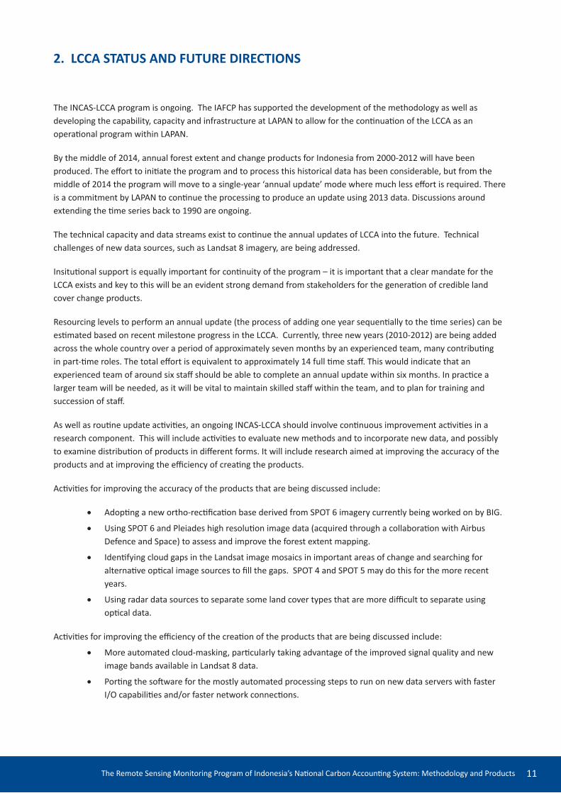
Aciviies for improving the accuracy of the products that are being discussed include:
• Adoping a new ortho-reciicaion base derived from SPOT 6 imagery currently being worked on by BIG.
• Using SPOT 6 and Pleiades high resoluion image data (acquired through a collaboraion with Airbus Defence and Space) to assess and improve the forest extent mapping.
• Idenifying cloud gaps in the Landsat image mosaics in important areas of change and searching for alternaive opical image sources to ill the gaps. SPOT 4 and SPOT 5 may do this for the more recent years.
• Using radar data sources to separate some land cover types that are more diicult to separate using opical data.
Aciviies for improving the eiciency of the creaion of the products that are being discussed include:
• More automated cloud-masking, paricularly taking advantage of the improved signal quality and new image bands available in Landsat 8 data.
• Poring the sotware for the mostly automated processing steps to run on new data servers with faster I/O capabiliies and/or faster network connecions.

The Remote Sensing Monitoring Program of Indonesia’s Naional Carbon Accouning System: Methodology and Products12
To guide the coninuous improvement process, feedback from the data users and data processing team should be sought to idenify the issues that have the biggest efect on the eiciency or suitability of the products. Research tasks will be designed to develop and test new methods against the current results for both accuracy and eiciency. If new methods, or new data sources, prove to be beter, training in the new processing will be provided to the processing teams and the operaional methodology updated. This cycle of evaluaing, tesing and improving can be coninued throughout the program life.
In parallel with improving the methodology, the infrastructure for data processing, data archiving and data delivery should be reviewed. Substanial improvements in technology have already been adopted in the LCCA through developments in LAPAN’s Remote Sensing Technology and Data Centre. Muli-CPU blade server computaional technology has become available for the most computaionally intensive steps in the processing and the data archive is being transferred to new, faster servers in the Data Centre.
There is also a need to educate the user community about the current products – their strengths and limitaions for paricular purposes and seek feedback on how best to deliver informaion products for applicaions other than the original carbon accouning purpose.
The INCAS-LCCA is one of a number of programs being developed for forest monitoring purposes both within and outside Indonesia. A formal accuracy assessment process should be developed to compare diferent products, noing that they will most likely have diferent purposes and diferent policy drivers. For example, LAPAN are developing a rapid response, ‘early warning’ forest detecion methodology. The temporal resoluion is much iner and the spaial resoluion is much coarser than the INCAS-LCCA. The accuracy requirement is also lower. All areas of possible forest clearing are detected and provided to local/regional agencies for on-ground veriicaion. Only those areas that are conirmed by these sources are acted upon. Opportuniies for coordinaion and cooperaion between these two projects are being considered as well as with other research aciviies.
Finally, the LAPAN team now has the capability to consider developing new products to complement the current forest extent and annual change maps. Such developments must be undertaken in collaboraion with the other stakeholders, and will typically involve other data in addiion to remote sensing.
The Remote Sensing Monitoring Program of Indonesia’s Naional Carbon Accouning System: Methodology and Products 13
3. SAMPLE RESULTS
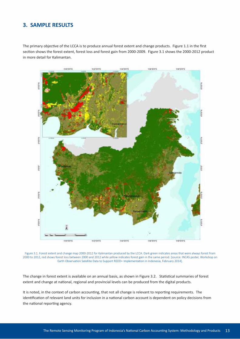
The primary objecive of the LCCA is to produce annual forest extent and change products. Figure 1.1 in the irst secion shows the forest extent, forest loss and forest gain from 2000-2009. Figure 3.1 shows the 2000-2012 product in more detail for Kalimantan.
Figure 3.1. Forest extent and change map 2000-2012 for Kalimantan produced by the LCCA. Dark green indicates areas that were always forest from
2000 to 2012, red shows forest loss between 2000 and 2012 while yellow indicates forest gain in the same period. [source: INCAS poster, Workshop on
Earth Observaion Satellite Data to Support REDD+ Implementaion in Indonesia, February 2014].
The change in forest extent is available on an annual basis, as shown in Figure 3.2. Staisical summaries of forest extent and change at naional, regional and provincial levels can be produced from the digital products.
It is noted, in the context of carbon accouning, that not all change is relevant to reporing requirements. The ideniicaion of relevant land units for inclusion in a naional carbon account is dependent on policy decisions from the naional reporing agency.

The Remote Sensing Monitoring Program of Indonesia’s Naional Carbon Accouning System: Methodology and Products14
Some of the datasets assembled during the LCCA processing are useful products for a range of other applicaions. The individual geometrically and radiometrically corrected images are available along with corresponding cloud masks. Regional and naional mosaics are also available. An example is shown in igure 3.3.
Figure 3.2. Forest extent and change map 2000-2012 for a region in Central Kalimantan produced by the LCCA. Dark green indicates areas that were
always forest from 2000 to 2012, shades of red, orange, yellow and pink show forest loss between 2000 and 2012. Each shade corresponds to a
diferent year (e.g 2000-2001, 2001-2002, ... , 2011-2012). Shades of green, blue and purple indicate reforestaion in the same period. [source: INCAS poster, Workshop on Earth Observaion Satellite Data to Support REDD+ Implementaion in Indonesia, February 2014].
Figure 3.3. 2007 Landsat mosaic of Nusa Tenggara with bands 3,4,5 in BGR. The area shown is approximately 1500km by 500km. Black areas within the islands indicate areas of missing data due to cloud in 2007.

The Remote Sensing Monitoring Program of Indonesia’s Naional Carbon Accouning System: Methodology and Products 15
Figure 4.1. Flowchart of the steps in the INCAS-LCCA processing sequence. The steps in blue form the data preparaion processing performed on individual images. The steps in orange form the forest extent and change mapping processing performed on the image mosaics. Ater every step a
quality assurance process is performed to check the accuracy of that processing step. If accuracy requirements are not met, the data is reprocessed. The inal step is a review of the products.
4. OVERVIEW OF OPERATING METHODOLOGY
There are a number of steps to produce the annual forest extent and change maps; the outputs from each step typically are required inputs for the subsequent step. The progression of processing steps is shown in the lowchart in Figure 4.1. Each of these steps is described in greater detail in secions below.
First the images to be used in the LCCA are selected. Not every image available in archives is suitable or needed for the processing. The selected images must be aligned geographically to each other and to other map data. Correcions to make the image values more consistent through ime are then made. Contaminaing data – such as cloud and shadow, haze, smoke and image noise - that obscure the ground cover are then masked from the images. The individual images are then mosaiced into larger units – mosaic iles – to streamline the subsequent processing. Together these steps form the data preparaion stage of the processing (Secion 6 below). These preparaions make the image data suitable for use for a range of applicaions.
There are three steps to making the annual forest extent and change products from the image mosaics (Secion 7). Firstly ground-truth data – expert knowledge and high resoluion images – are used to associate the image signals with forest and not forest cover to create a forest base for a single year in a very hands-on approach. Then a semi-automated matching process is used to ‘match’ the data for other years to the base. In the inal step, knowledge of the temporal growth paterns in forest and non-forest cover types is used in a mathemaical model to reine the single-date results to provide more reliable change detecion.

The Remote Sensing Monitoring Program of Indonesia’s Naional Carbon Accouning System: Methodology and Products16
The inal step in the processing is to review the products, both to gain feedback on their accuracy and to understand their strengths and limitaions for paricular purposes. This review can suggest strategies for improving the products in the future.
Ater each step in the processing there is a quality assurance (QA) process to check that the method has been correctly applied and that the results meet required accuracy standards. If an image does not meet the standards for that step, the cause is invesigated and the image reprocessed to correct the problem and checked again. The next step is not commenced unil the current step is successfully completed. The quality assurance checks also ensure consistency between data processed by diferent team members and at diferent imes during the project.
An image database idenifying each selected image is created. This is used to track the progress of each image through the data preparaion and quality assurance checks. Summary informaion from this database is used to report overall progress and idenify botlenecks or delays in the processing. The imely creaion of the products relies on good management of the processing using such data.
A comprehensive data archive has been created in the LAPAN Data Centre for the LCCA. Systemaic archives are created for output images and products for each processing step. The archive includes processing iles which enable each step of the processing to be audited, and reproduced if necessary. The product archive includes a full record of each version of the processing; both the original 2000-2009 products and the improved and updated 2000-2012 products are archived so that any version of the products can be reproduced.
A processing team with experience in the use of satellite imagery has been trained to perform the processing steps and the quality assurance checks using the methodology described in this document, as per the detailed instrucions in the ‘Operaional Manual’. Some team members specialise in paricular steps and are able to train new team members. This ability to learn then teach the processing methodology is paricularly important in long-running operaional programs as some people will move on to other aciviies and be replaced by new team members. This dedicated image analysis team is supported by people with local knowledge of the land cover in each region when the forest base is created. These local experts do not need experience with satellite imagery, although it is an advantage.

The Remote Sensing Monitoring Program of Indonesia’s Naional Carbon Accouning System: Methodology and Products 17
5. SOURCES OF DATA AND INFORMATION
5.1 Landsat imagery
As noted in Secion 1, Landsat imagery was chosen as the only feasible data source to provide monitoring informaion for the implementaion of LCCA. Landsat 5 (LS-5) and Landsat 7 (LS-7) were operaional in the period. LS-5 is the preferred source for most of the period due to a technical problem with the scan line corrector (‘SLC-of’) which afected LS-7 from mid-2003. However in cases where cloud cover afects available LS-5 imagery, LS-7 imagery may be more useful. Both instruments have collected regular repeat coverage every 16 days over the period, but not all overpasses had been received and archived. Due to the frequency of cloud coverage over Indonesia, and other data quality problems it was desirable to have access to the most complete archive possible prior to selecion of scenes for the LCCA (see Secion 6.1 for descripion of scene selecion).
The most complete archive of LS-5 imagery for western Indonesia for the period was held at Thailand’s GISTDA receiving staion; Australia’s archive, held at Geoscience Australia (GA) covers far eastern Indonesia (Papua to eastern Nusa Tenggara) with LS-5 and LS-7 imagery. LAPAN’s receiving staion at Parepare covers all of Indonesia, except for the very western ip of Sumatra, but only limited scenes had been archived. The main source of data for the central region was thus the USGS archive, which was far from complete for LS-5 as it consists of a sample of scenes selected for on-board storage and downloaded in the US. GA coordinated the image acquisiion of Landsat imagery from these internaional data agencies in collaboraion with the LCCA scene selecion process described in Secion 6.1. All selected data was delivered to Indonesia for processing within LCCA. Secion 6.1 also provides detail on the numbers of scenes sourced from these various archives.
Figure 5.1. Indicaive extent of spaial coverage of the GISTDA and GA Landsat archives. Lapan’s receiving staion recepion disk covers the full extent of Indonesia except for the northwest ip of Sumatra.
With respect to more recent and future data, it should be noted that the data recepion, archiving and availability in Indonesia has advanced dramaically since the LCCA commenced. In part this progress is a result of the experience in implemening the LCCA. Landsat 8 (LS-8) is now operaional and complete coverage of Indonesia including western Sumatra is received, archived and rouinely ortho-reciied by LAPAN. This has arisen through collaboraion with USGS which has assisted LAPAN in implemening an internaional-standard processing stream for the imagery. LAPAN has also negoiated recepion of higher resoluion SPOT-4, SPOT-5, SPOT-6 and Pleiades imagery in collaboraion with Airbus Defence and Space.

The Remote Sensing Monitoring Program of Indonesia’s Naional Carbon Accouning System: Methodology and Products18
5.2 High resoluion imagery
Samples of high resoluion satellite imagery were acquired for the LCCA. These were used for purposes of accurate interpretaion of land cover in the forest mapping and forest review stages of the program. These tasks required an image resoluion which could provide esimates of tree density, and indicaions of height from shadow. A resoluion of two metres or beter is required for these purposes. Air photography was not available, so commercial high resoluion satellite imagery provided the only opion.
Limited archives were available at the ime from the Ikonos satellite (which commenced operaion in 2006), GEO-eye, Quickbird and WorldView satellites. With addiional support from IAFCP, samples of high resoluion imagery were purchased over Kalimantan, Sumatra, Papua and Sulawesi for the forest base workshops conducted in 2011-2012. The criteria for image selecion and the uses of the data are described in Secion 6.2 below and in Secion 7. All data were purchased with a muli-user licence which allowed distribuion of copies to GoI agencies including LAPAN, MoF, BIG and the Presidenial Working Unit for Supervision and Management of Development (UKP4). Further detail on the number and locaion of images is found in Secion 6.2. Images were not purchased by the program for the remaining regions of Indonesia due to developments in data policy and data availability as described in Secion 6.1.
5.3 Expert knowledge and map data
Informaion from experts with knowledge of regional land cover and land use was a criical input to the forest base mapping (Secion 7.1) and product review (Secion 8) as successive regions were processed. Typically three to ive ground experts formed part of the base mapping team for each region. The MoF assisted with provision of its staf and with suggesions for regionally based experts. Staf from BIG also assisted in this role for all regions. These ground experts were asked to bring any relevant exising GIS data, maps or ground site informaion to assist in the forest mapping processes. In combinaion with the high resoluion imagery, and the available maps, this human experise with regional knowledge provided essenial guidance to the producion and assessment of the forest extent base maps.

The Remote Sensing Monitoring Program of Indonesia’s Naional Carbon Accouning System: Methodology and Products 19
6. DETAILED METHODOLOGY – IMAGE PREPARATION
This secion describes all stages of the selecion, processing and QA of Landsat scenes which are conducted prior to the forest extent mapping stages. The products from the image preparaion stages used in subsequent steps of LCCA are corrected annual mosaic images for all regions of Indonesia. Products produced within the image preparaion include ortho-reciied and radiometrically corrected individual scenes, and processing iles which record the details of all processing steps and which are suicient to provide an audit record of the numerical processing, and to reproduce each step if required. All such iles are in the LCCA archive at LAPAN.
6.1 Scene selecion
To map annual forest extent and change we require one cloud-free view of the land cover each calendar year. A single clear image is ideal and suicient, but due to cloud cover this is a rare occurrence in tropical regions like Indonesia. The aim of the scene selecion is to provide annual coverages of Indonesia with maximum cloud-free land area using the minimum number of scenes. The selecion criteria were designed to provide best inputs to the subsequent forest extent mapping process. The speciicaions allow for selecion of several images within each path/row to achieve a composite mosaic for each year, but this number is limited in anicipaion of the manual efort required in parts of the image preparaion processing.
The land area of Indonesia is covered by approximately 220 Landsat scenes (Figure 6.1.1) from paths 100-131. Many of these scenes include large areas of water. The Landsat satellite revisits each orbit path every 16 days, so where the archive is complete, there are approximately twenty-two images per year for each path/row to choose from. The historic archives available to the LCCA typically contain less than this as described in Secion 5.
Figure 6.1.1. Landsat path/row coverage of Indonesia
Image selecion is best done by visual assessment of high-quality browse images. The full set of browse images from the archives described in Secion 5 was provided to the LCCA and is archived. Experience tells us that image cloud cover staisics typically provided with browse images are unreliable for scene selecion. The summary staisics do not provide any informaion on the spaial distribuion of the cloud in an image – and this is an important consideraion. For example, an image with 50% cloud cover all in the north will be usable in the south and easy to ‘cloud mask’. An

The Remote Sensing Monitoring Program of Indonesia’s Naional Carbon Accouning System: Methodology and Products20
image with patchy 50% cloud over the whole scene is likely to be contaminated by atmospheric efects and shadow and diicult to mask and use. More obviously, in images covering small islands, a small proporion of cloud over the land areas may make an image useless for LCCA purposes, while cloud areas over ocean are irrelevant.
To make the image selecion, all image dates for the paricular path/row and calendar year should be available as high-quality browse images. The best images are those that are completely free of any data problems, and which provide the best discriminaion of forest cover. Besides cloud cover, other data quality issues include, but are not limited to, data errors (e.g. line drop-out), smoke and extensive looding.
Sensor quality is also considered. Prior to August 1999, Landsat 5 is the only opion. Unil the Landsat 7 scan line corrector (SLC-of) problem, LS-5 and LS-7 both provide suitable imagery. LS-7 is the preferred choice where cloud and other data quality issues are acceptable. From July 2003, all LS-7 images have the SLC-of problem producing stripes of missing data. The preference is for LS-5 imagery, but where cloud problems are signiicant LS-7 images are considered. Between November 2011 and June 2013 only LS-7 SLC-of data is available. From July 2013, Landsat 8 is the preferred sensor.
In most parts of Indonesia for most years, cloud-free land area is the primary consideraion for selecion. Where there is a choice of cloud-free images, the ime of year of the available images can also be considered. In many regions images from the dry season provide best discriminaion between forest and non-forest land cover and are chosen where possible. In parts of Java and Nusa Tenggara the forest is deciduous, losing its leaves in the dry season, and images from a slightly weter ime are preferred.
Early in the project, the processing level of the source images was also considered. Path level images (L1G – nominal orientaion) were preferred over automaically ortho-reciied images (L1T) as the accuracy and reliability of the L1T products did not meet the registraion speciicaions. Over the life of the project, the automated processing systems have improved and processing level is less of an issue.
Generally, for each path/row and year up to 4 scenes are selected; more are considered with LS-7 SLC-of data and in areas where cloud-free imagery is known to be rare. A ‘primary’ image is selected with the biggest coniguous cloud-free areas. If this scene is completely cloud free over land areas, then no further images are required for that path/row and year. All subsequent images are chosen to complement the primary image, i.e. have clear data where the primary is cloudy, to build the composite with maximum cloud-free area. Where choice exists, temporal consistency down paths and close dates across rows are preferred. Haze requires atenion – it is not always clearly visible in the browse imagery.
As an example of applying the scene selecion criteria, Figure 6.1.2 shows the browse images for all available LS-5 scenes for path/row 100/065 in 2004. LS-5 is the preferred opion as LS-7 is SLC-of. Clearly, cloud or data problems afect many images.

The Remote Sensing Monitoring Program of Indonesia’s Naional Carbon Accouning System: Methodology and Products 21
Figure 6.1.2. Browse images for all available LS-5 images in path/row 100/065 in 2004.
Figure 6.1.3 shows the three most likely candidate images for selecion in more detail. The irst candidate image is cloud-free in the north-east and approximately 70% cloud free in the south. The cloud in the north-west is in large patches rather than scatered which is easier to mask. Close inspecion of the second candidate image shows that although the south appears cloud-free in the thumbnail, there is evidence of haze (bluish-purple smudges) in the larger view. The third candidate image is clear in the south and also in the central west where the irst candidate image is cloudy. Together the irst and third candidate images provide cloud free coverage for nearly the enire scene. The north-west has remaining areas of cloud. The review of the remaining browse images concentrates on this region. Unfortunately there are no candidates that ix this and so the scene selecion stays at two for this path/row in 2004.

The Remote Sensing Monitoring Program of Indonesia’s Naional Carbon Accouning System: Methodology and Products22
Candidate image 1 (12 Feb 2004) - top row
centre in Figure 6.1.2
Candidate image 2 (9 Sep 2004) – 3rd
row right in
Figure 6.1.2
Candidate image 3 (22 Aug 2004) – 4th
row
centre in Figure 6.1.2
Figure 6.1.3. The three most clear browse images for 100/65 in 2004.
The result of the scene selecion process is a list of images to be used – for each path/row for each year. Large areas with no clear imagery can also be noted. For QA, the list of selecions and the full set of browse images can be passed to another person for review.
Once the scene selecions are inal, the full versions of the selected images are obtained from the diferent source archives, each with their own data formats, and imported into a standard format for subsequent processing. The list of images is imported into the INCAS-LCCA database. This database records informaion about the image – locaion, date, and source – and monitors the progress of processing through the image preparaion and QA steps. Figure 6.1.4 shows a snapshot of part of the database and Figure 6.1.5 shows a summary report derived from the database.

The Remote Sensing Monitoring Program of Indonesia’s Naional Carbon Accouning System: Methodology and Products 23
Figure 6.1.4: Snapshot of a page of the image database. As well as idenifying all of the images selected, it tracks the process of the image through each processing and QA step.
Figure 6.1.5. Sample summary reports derived from the database for tracking progress at a management level.

The Remote Sensing Monitoring Program of Indonesia’s Naional Carbon Accouning System: Methodology and Products24
Summaries of the images used in the INCAS–LCCA can be extracted from this database. Figure 6.1.6 illustrates the number of images selected for each path/row across Indonesia in 2008. A small number of images over land areas indicates either that good clear images are available, or that few suitable images are available. The amount of clear land (ater cloud masking) that results from these selecions is shown in the mosaicing secion (Secion 6.7) of this document. Figure 6.1.7 provides a summary of the numbers of images by region.
Figure 6.1.6. Number of images selected for 2008. White shows no suitable data available, red shows one selected image, yellow shows two selected
images, blue shows three selected images and green shows four or more selected images.
Figure 6.1.7. Number of Landsat images selected for each year from 2000-2009 across Indonesia
As at April 2014, there are 6553 Landsat images in the INCAS-LCCA archive for years 2000 to 2012. The Landsat image data was sourced from three outside archives (Thailand (GISTDA) – 893 scenes, Australia (GA) – 974 scenes, the United States of America (USGS) – 4436 scenes, as well as the Indonesian (LAPAN) archive – 250 scenes. For images acquired from December 2012, the LAPAN archive will be the primary data source.

The Remote Sensing Monitoring Program of Indonesia’s Naional Carbon Accouning System: Methodology and Products 25
Figure 6.2.1: Landsat and high resoluion imagery for a sample area in central Kalimantan. Top let: 2009 Landsat TM image (25m) bands 3,4,5 in BGR. Top right: Pan-sharpened SPOT 5 image (2.5 and 10m). Botom-let: Pan-sharpened SPOT 6 (1.5m). Botom-right: Pan-sharpened Quickbird
(0.6m and 2m). Individual trees can be seen in the Quickbird and SPOT 6 imagery which is suitable for LCCA purposes. Land cover can be inferred from the SPOT 5 imagery but more interpretaion is required.
6.2 High resoluion imagery
Ground-truth informaion for training the forest extent mapping and for accuracy assessment is provided by local experts from each region of Indonesia. This is assisted by the interpretaion of high resoluion imagery.
The resoluion, locaion and date of acquisiion determine the usefulness of high resoluion imagery for INCAS-LCCA. Visible and near infra-red imagery is suitable for determining land cover. Higher spectral resoluion is of limited value for this purpose.
The spaial resoluion must be ine enough to idenify individual tree crowns and land use types. In ine resoluion imagery the presence, or absence, of disinct shadows give an indicaion of vegetaion height. A spaial resoluion of 2m or iner is required. Suitable sources of imagery include aerial photography (variable), IKONOS (approx 4m muli-spectral, approx 1m panchromaic), Quickbird, WorldView 2, GeoEye1, Pleiades (approx 2m muli-spectral, 0.5m panchromaic) and Spot 6 (1.5m muli-spectral and panchromaic). Other sources such as SPOT-5 (10m muli-spectral, 5m regular panchromaic or 2.5m super mode panchromaic), ALOS (10m muli-spectral (AVNIR) and 2.5m panchromaic (PRISM)) and RapidEye (6.5m) are less suitable for idenifying trees and tree height, but may be useful for broad land cover interpretaion. Figure 6.2.1 shows some sample imagery.
For INCAS-LCCA forest extent mapping purposes, image dates closest in ime to the date of the Landsat mosaic chosen for the ‘forest base’ are the most useful (Secion 7.1). 2008 is generally the target year as it was the most recent for which Landsat mosaics were produced at the ime the forest processing started. Choosing a recent year allows access to local memory of land cover and condiion from site visits rather than having to rely exclusively on high resoluion imagery for developing the classiicaion.

The Remote Sensing Monitoring Program of Indonesia’s Naional Carbon Accouning System: Methodology and Products26
High resoluion imagery is expensive to acquire and archives do not provide complete coverage. Sample images in key locaions were selected in locaions which were best for the purpose, considering images already held by GoI. At the beginning of the project litle high resoluion data was available. Images were selected and purchased by IAFCP for the INCAS-LCCA for Kalimantan, Sumatra, Papua and Sulawesi. For Java, imagery that had been purchased by the Ministry of Agriculture was available for use by LAPAN– the coverage is shown in Figure 6.2.2. Similar imagery held for Nusa Tenggara could not be used because of license restricions. Extensive use was also made of the imagery available in Google Earth(TM) for Java and Nusa Tenggara. The resoluion of the imagery in Google Earth(TM) varies signiicantly, but is high for much of Java and parts of Nusa Tenggara. Litle high resoluion imagery is available for Maluku, either commercially or publicly, and more emphasis was placed on seeking local expert input.
The high resoluion images for Kalimantan, Sumatra, Papua and Sulawesi were selected to contain cloud-free samples of all important cover types. It is important that the images contain muliple cover types and/or a mixture of tree density so that boundaries between land cover classes can be interpreted. Extra images were purchased in areas of rapid change and uncertainty about cover type. High resoluion image locaions were selected by comparing a browse library of available images to the LCCA Landsat mosaics. Locaions were selected with high local variability in the Landsat mosaics (muliple cover types) and relaively clear data in the high resoluion imagery. As many land cover types and groupings were covered as possible within budget limitaions. Figure 6.2.3 shows the high-resoluion image locaions for the four regions. In total, 271 high resoluion images were purchased for the LCCA.
Figure 6.2.2. Locaions of IKONOS (red) and GeoEye1 (light blue) imagery for Java available to LAPAN from the Ministry of Agriculture; background: 2008 Landsat TM mosaic (bands 3, 4, 5 in BGR).

The Remote Sensing Monitoring Program of Indonesia’s Naional Carbon Accouning System: Methodology and Products 27
Figure 6.2.3. Locaions and numbers of high resoluion imagery (closed red squares) provided by IAFCP for four regions shown on 2008 Landsat TM mosaics (bands 3, 4, 5 in BGR). The open red and blue polygons show the locaions of high resoluion imagery already held by LAPAN.
Sumatra:
77 Quickbird, Ikonos, World View-2 (2006 to 2009).
Kalimantan:
53 Quickbird, Ikonos, World View-2, and Geo Eye-1
(2001 to 2010, mostly 2007 to 2009).
Papua:
62 Quickbird, Ikonos, World View-2, and GeoEye
(2006 to 2011).
Sulawesi:
79 Quickbird and World View-2 (2006 to 2011).

The Remote Sensing Monitoring Program of Indonesia’s Naional Carbon Accouning System: Methodology and Products28
6.3 Geometric base and correcion
In recent years there have been rapid developments in programs to improve the availability and standards of reciied Landsat imagery. At the ime of INCAS planning and commencement this was not the case; selecion of a geometric reference base for Indonesia, and procedures for accurate geometric correcion were recognised as of basic importance.
Accurate scene registraion within and between years is essenial for a monitoring program so that misregistraion errors are not confused with land cover change (Townshend et al. 1992). The efects of misregistraion in the ime series of imagery are illustrated in Figure 6.3.1. Forest versus not forest maps from two years are compared to idenify change. The two maps are well registered in the picture on let and one map has been shited one pixel to the right and one pixel down in the picture on the right. The small and narrow areas of change indicated on the let image are likely to be correct, while more false change (due to misregistraion) is shown on the right. Although the net area of land cover change (total clearing subtract total regrowth) would be the same, the maps and staisics of change from the misregistered image pair would be incorrect, and unsuitable for carbon accouning.
Figure 6.3.1. A comparison of forest and change maps from two ime periods. The two images which produced the let map were well registered; the pair on the right have been produced from the same images where one has been shited to simulate misregistraion efects on the change maps.
Automated, or at least semi-automated, generaion of ground control points (GCPs) by comparing a new image base to an agreed base image is the most eicient way of achieving good image to image registraion. Ideally the base imagery would have high locaional accuracy so that the image data can be compared to spaially referenced data from other sources.
As the equator passes through Indonesia a decision needed to be made within the LCCA about the projecion for the individual images. For convenience and consistency all images within the LCCA are referenced to NUTM coordinates (WGS84 datum). In NUTM zones, the equator has a northing coordinate of zero. Areas south of the equator within the the LCCA thus have negaive coordinates. If conversion to SUTM is required for any reason, only a simple constant shit (or ofset) in northing is required. All images are resampled to 25m pixel size for simple alignment with metric map scales and area calculaions. The inal products are converted to geodeic projecion to allow mosaicing across the whole country. A pixel size of 0.00025 degrees is selected.

The Remote Sensing Monitoring Program of Indonesia’s Naional Carbon Accouning System: Methodology and Products 29
6.3.1 Ortho-reciicaion base and digital elevaion model
There was no GoI ortho-reciicaion image base for the whole of Indonesia when this project started in 2009. Therefore the Global Land Survey 2000 (GLS2000) data (USGS 2009, htp://glcf.umd.edu/data/gls/) was selected for
this purpose. The GLS2000 is formed from Landsat 7 ETM+ images and is a reprocessed version of the Global Land Cover Facility (GLCF) 2000 GeoCover(TM) collecion (Tucker et al 2004) using Shutle Radar Topography Mission (SRTM) digital topography and improved geodeic control (Gutman et al. 2008). The data is provided in GeoTIFF format with a UTM projecion using the WGS-84 datum at 30m pixel resoluion.
Individual images comprising GLS2000 were downloaded from the USGS by GA in May and June 2009 and mosaiced together within UTM zones. The associated metadata ideniies the images as:
PRODUCT_NAME = “GLS-2000 Ver1.0”
PRODUCT_ELEVATION_DATA = “GLS-DEM Ver1.0”
The 2000 GeoCover(TM) product has been assessed as having a locaional accuracy RMS error of 50m. Subsequent studies suggest that some images may exhibit errors considerably greater than 40-50m, paricularly over mountainous areas and where the original DEM was of poor quality. The GLS2000 product was designed to address these limitaions.
Some isolated image-to-image misregistraion was discovered in adjoining images in parts of Indonesia during the INCAS–LCCA processing. In such regions, a new image for one or both path/rows was carefully processed and the well-registered images used to correct (overwrite) the GLS2000 product locally. Some parts of the GLS2000 base are quite cloudy. A mosaic was formed from cloud-masked images of Papua that have been processed as part of this project and used to replace cloudy data in the base for the LCCA.
At the present ime the issue of a more accurate Indonesian ortho-reciicaion base is being pursued as part of other GoI projects. Once a new base is established, a transformaion from the current LCCA base to the new one can be established for each region and the essenial data and products transformed.
The digital elevaion model (DEM) used in the ortho-reciicaion processing is the SRTM-DEM version 3 at 90m pixel resoluion, downloaded in May 2009. It is also used in the terrain-illuminaion correct step.
6.3.2 Correlaion matching and Master ground control points
To register a new image to the base, correlaion matching is used to locate predeined physical features from the ortho-reciied base image in the new image. The coordinates of the center of these features are then used as the GCPs to formulate the transformaion between the new image and the base.
A library of these predeined feature locaions was created for every path/row for Indonesia. In the INCAS-LCCA these locaions are called ‘Master GCPs’. They are also referred to as ‘GCP chips’ in some applicaions. The later terminology usually refers to a small image window or subset (say 64 lines by 64 pixels) that is stored in a database. In the LCCA, only the feature locaion is stored and the data from the image window is read from the base image as required during processing. This allows lexibility in the feature window size.
Tradiionally, GCPs were points, such as a road intersecion or a sharp corner of some region, which could be uniquely indeniied in two images or in an image and a map. GCP features for correlaion matching are larger clear physical shapes that can be ideniied in two images. If the images shapes are on top of each other, the correlaion between the image windows is high. If the shapes are slightly shited in any direcion, the correlaion between the image windows is lower. The higher the contrast between the shape and the background, the more quickly the correlaion

The Remote Sensing Monitoring Program of Indonesia’s Naional Carbon Accouning System: Methodology and Products30
will decrease (or the more subtle a shit that can be detected). The shape must also be disinct in both east-west and north-south direcions so that the change in correlaion will be sensiive to misregistraion in any direcion. The shape must also be big enough compared to the window size to dominate in the correlaion calculaions. In the LCCA, Master GCP features are ideniied as the centre point of a ten line by ten pixel window. Figure 6.3.2 shows some examples of Master GCP features.
In correlaion matching to locate the feature in a new image, the locaion to search for each feature is restricted to a twenty line by twenty pixel window around coordinates predicted by a simple linear relaionship ited to a small number of manually located staring GCPs. This is eicient computaionally but also minimizes false matches to features with a similar shape elsewhere within the image.
Figure 6.3.2. Some examples of Master GCP features from Kalimantan that are used in the correlaion matching to generate GCPs. The whole region inside the yellow box forms the feature window. Band 7 of the ortho-reciicaion base image is shown in this display, but the correlaion is performed
over several image bands.
The Master GCPs used in the LCCA were collected manually by visual inspecion of the mosaiced ortho-reciicaion base images. As well as being disinct shapes with high contrast to the background, Master GCPs also need to be features that are stable through ime so that they can be used with any image dates. For example, natural clearings in a forest created by rocky outcrops are beter than the edge of forest nearest to expanding agricultural lands. A disinct curve or peninsular in a rocky coastline is beter than part of the waterline on a wide beach with a big idal range. A bend in a river in the mountains that is ightly constrained by terrain is beter than a bend in the same river in the low lat lands where looding over successive wet seasons can change the main channel.

The Remote Sensing Monitoring Program of Indonesia’s Naional Carbon Accouning System: Methodology and Products 31
GCP chips were also obtained from USGS at the same ime as the GLS2000 data was downloaded and evaluated for use in the LCCA. Inspecion of these chips showed that many were ire fronts. They had very high spectral contrast within the chip image date, but no temporal stability and so were unsuitable for the LCCA. As a result, the LCCA adopted a manual selecion process as described above. As locaing Master GCP selecion needs to be done once only, adoping a manual approach did not impose a high overhead.
A Master GCP ile for an image is a thus text ile which contains a list of geographic coordinates (easing and northing) in the UTM zone applicable for that image. The ile name records the path/row and the UTM zone to which it applies. Where images overlap UTM zone boundaries, Master GCP iles for both zones are stored.
Two sets of Master GCPs were selected. One – the Master Registraion GCPs – serve to generate ground control points for iing the ortho-reciicaion model, as described in the next secion. The other – the Master Check GCPs – serve as sets of independent check points that are used during the quality assurance stage to assess how well the processed image is registered to the base. Typically about 100 points for each image were selected for Master Registraion GCPs, and about 60 for Master Check GCP’s. These numbers (if all are matched) are more than required for registraion, but condiions in Indonesia (especially cloud) required such numbers for eicient reciicaion processing (below). The Master Registraion GCP iles and Master Check GCP iles for all images are stored in the LCCA archive at LAPAN.
6.3.3 Ortho-reciicaion of individual images
Prior to subsequent processing in the LCCA, all Landsat images must be ortho-reciied and registered to the geometric base. The aim of this process is to produce individually reciied images, which will eventually result in a consistently-registered ime series of imagery for all of Indonesia. As noted in Secion 6.1, historic images were provided from diferent archives and with diferent levels of processing. The preferred processing level for historic imagery was path-oriented (nominal orientaion) to enable full ortho-reciicaion correcion within LCCA. Path-oriented images are referred to as ‘raw’ images in this secion. In some cases, selected images were only available as Level 1T (L1T) ortho-corrected. This secion describes the ortho-reciicaion process for path images. L1T images at the ime were generally not registered to the base to LCCA standards and reprocessing was oten required. Processing for these L1T images is also described below.
The ortho-reciicaion processing applies correlaion matching to ind in the overpass image the pixel locaions which correspond to the base coordinate locaions in the Master GCP ile. The correlaion calculaions are performed using image bands 3, 4 5, and 7. Details of operator inputs to this process are described below. The result is a new ile of GCP points for the speciic image which contains only well-matched GCP locaions in base map and raw image coordinates. Heights of the selected GCPs are then found from the DEM and atached.
These selected points are used in a single program (‘geo-correct’) which its a sequence of three models in the actual ortho-reciicaion process of the raw image. The details are found in Wu (2008). This approach achieves accurate ortho-reciicaion without the requirement for sensor and orbital ephemeris informaion, only an approximate satellite height. The approach has been compared to established implementaions using satellite orbital modelling and results agree very closely; for LCCA purposes they are idenical. The resampling kernel used is 16-point sinc with Kaiser windowing.
The inputs to ortho-reciicaion are a raw overpass image, the base mosaic for the appropriate NUTM zone, the corresponding DEM, and the Master Registraion GCP ile for the overpass image. The major outputs are the ortho-reciied image, and the new inal reciicaion GCP ile with heights which was used. Other iles including the interim GCP iles and iles providing diagnosics on the model iing are also produced and forwarded for QA. Within the LCCA, sotware has been developed by LAPAN to simplify the operator processing and the generaion of diagnosics for QA.
The Remote Sensing Monitoring Program of Indonesia’s Naional Carbon Accouning System: Methodology and Products32
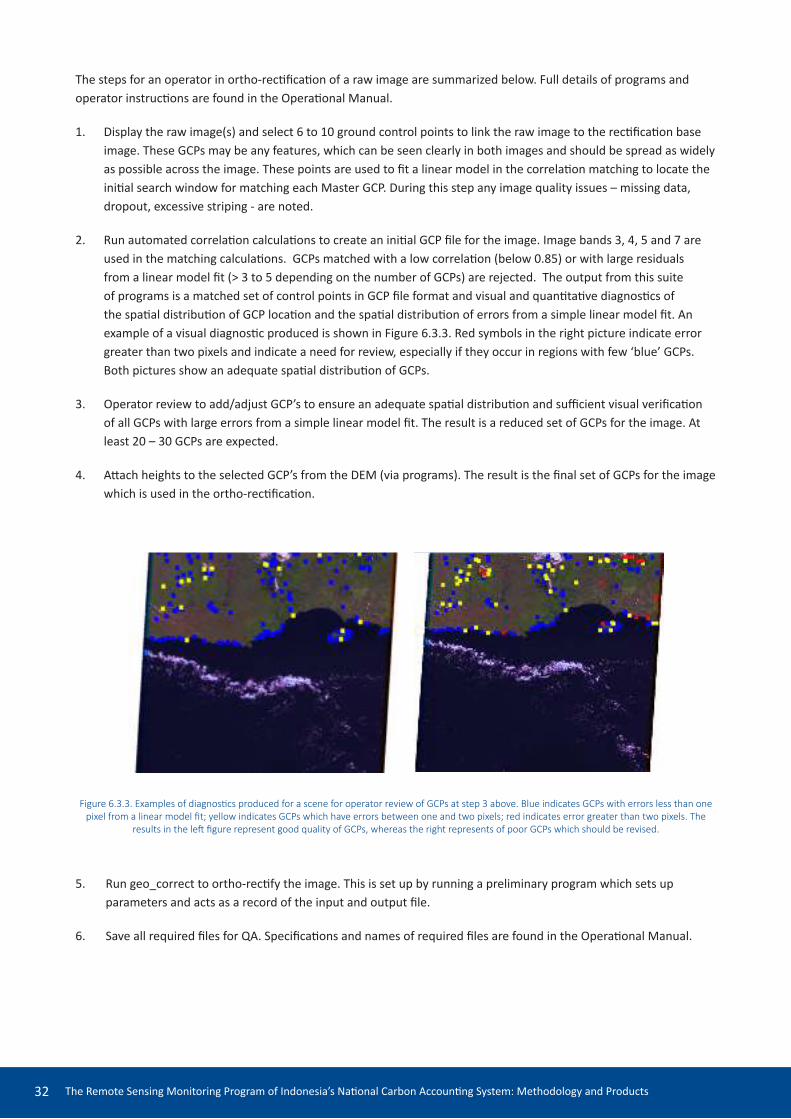
The steps for an operator in ortho-reciicaion of a raw image are summarized below. Full details of programs and operator instrucions are found in the Operaional Manual.
1. Display the raw image(s) and select 6 to 10 ground control points to link the raw image to the reciicaion base image. These GCPs may be any features, which can be seen clearly in both images and should be spread as widely as possible across the image. These points are used to it a linear model in the correlaion matching to locate the iniial search window for matching each Master GCP. During this step any image quality issues – missing data, dropout, excessive striping - are noted.
2. Run automated correlaion calculaions to create an iniial GCP ile for the image. Image bands 3, 4, 5 and 7 are used in the matching calculaions. GCPs matched with a low correlaion (below 0.85) or with large residuals from a linear model it (> 3 to 5 depending on the number of GCPs) are rejected. The output from this suite of programs is a matched set of control points in GCP ile format and visual and quanitaive diagnosics of the spaial distribuion of GCP locaion and the spaial distribuion of errors from a simple linear model it. An example of a visual diagnosic produced is shown in Figure 6.3.3. Red symbols in the right picture indicate error greater than two pixels and indicate a need for review, especially if they occur in regions with few ‘blue’ GCPs. Both pictures show an adequate spaial distribuion of GCPs.
3. Operator review to add/adjust GCP’s to ensure an adequate spaial distribuion and suicient visual veriicaion of all GCPs with large errors from a simple linear model it. The result is a reduced set of GCPs for the image. At least 20 – 30 GCPs are expected.
4. Atach heights to the selected GCP’s from the DEM (via programs). The result is the inal set of GCPs for the image which is used in the ortho-reciicaion.
Figure 6.3.3. Examples of diagnosics produced for a scene for operator review of GCPs at step 3 above. Blue indicates GCPs with errors less than one pixel from a linear model it; yellow indicates GCPs which have errors between one and two pixels; red indicates error greater than two pixels. The
results in the let igure represent good quality of GCPs, whereas the right represents of poor GCPs which should be revised.
5. Run geo_correct to ortho-recify the image. This is set up by running a preliminary program which sets up parameters and acts as a record of the input and output ile.
6. Save all required iles for QA. Speciicaions and names of required iles are found in the Operaional Manual.

The Remote Sensing Monitoring Program of Indonesia’s Naional Carbon Accouning System: Methodology and Products 33
Images which were supplied as L1T have already been through an ortho-correcion process. Ater imporing they are resampled to 25m pixel size and the QA process applied as described below for the images ortho-reciied by the LCCA team. Approximately 80% of L1T images were well registered to the base, although this percentage was lower for images with only small islands or extensive cloud with only limited clear land area. If an L1T image was found to be poorly matched to the base, a set of GCPs was derived for the image manually. A linear model only was ited to these GCPs to re-recify and resample the image. QA was then performed on the new result. This was found to produce saisfactory results in nearly all cases. In recent years, the consistency of automated Landsat processing by USGS and other agencies has improved following feedback from the LCCA program to USGS. LAPAN has implemented USGS processing of Landsat images currently received in Indonesia, and it is anicipated that images from this processing will be also submited to the same QA process.
Ortho-reciicaion QA is carried out by a nominated group of independent staf. The inal result is criically dependent on the operator’s checking and decisions for the accepted GCPs during the processing. The requirement for acceptable registraion to the base is that the overall misregistraion be less than one pixel with no systemaic paterns in the shits between the new image and the base. For example, if the whole image is shited half a pixel to the right of the base, then the registraion is not acceptable even though the shit is less than one pixel. If the shits are in random direcions, overall residuals of half a pixel are acceptable.
The registraion is assessed both visually and quanitaively. The correlaion calculaions are repeated between the ortho-reciied image and the base image at Master Check GCP locaions. These check GCP locaions are independent of the Master Registraion GCP locaions. The size of the correlaion value and the size of the residuals from a simple linear it are used to exclude poorly matched features from the staisical summaries. The RMS error and pictures of the spaial distribuion of the well matched Check GCP locaions, size of shits and direcion of shits are produced – similar to those produced during the generaion of the original GCPs for the model iing. If these summaries show an acceptable registraion, only a quick visual inspecion is performed. If the summaries show possible problems a much more detailed visual inspecion is performed to diagnose the problem and suggest possible soluions.
The inal check of the reciied image is visual: one band of the reciied image (usually band 5 or 7) is overlaid on the corresponding band of the base in red and green, while standard image displays of both are viewed simultaneously. The QA operator will zoom to diferent parts of the image and check for any evidence of misregistraion in unchanged features; the standard image displays provide guidance on cloud and changes in land cover which may be ignored. An example of the two-image red-green visual display is shown in Figure 6.3.4. Here dark and yellow colours indicate dark and bright areas which are ‘unchanged’ in brightness; red and green tones indicate change in brightness at that locaion. The displacement of roads and river edge in the let image is clear evidence of misregistraion, while the right image appears well registered on these clear linear features. There are noiceable red areas in the river in the right image which would be carefully examined at QA. These are likely to result from changes in river level or turbidity rather than misregistraion, in which case QA would pass this porion of the image. Note also the red and green coloured areas which result from land cover change. Where an image fails QA, it is returned to the ortho stage with comments and pictures such as shown in this igure, to assist in reinement of the selected GCPs.

The Remote Sensing Monitoring Program of Indonesia’s Naional Carbon Accouning System: Methodology and Products34
Figure 6.3.4. Detail of ortho-reciicaion QA visual checking, using a display of a reciied image band and base image band in red and green. Dark and yellow colours indicate dark and bright areas which are ‘unchanged’; red and green tones indicate change in brightness at that locaion, The
displacement of roads and river edge in the let igure is evidence of misregistraion, while the right image does not show such displacement. The let ortho image would be failed at QA. These images are of Papua.
Archiving of iles is the inal stage of the ortho process; the iles to be archived are described in the Operaional Manual.

The Remote Sensing Monitoring Program of Indonesia’s Naional Carbon Accouning System: Methodology and Products 35
Figure 6.4.1. Detail of two overlapping images from south-west Java (bands 4,5,3 in RGB) before and ater correcion.
(a) image before TOA and BRDF correction
(b) Image after TOA and BRDF correction
6.4 Radiometric correcion - BRDF
The digital numbers recorded in Landsat images are afected by on-board processing parameters, the distance to the radiaion source (the sun), angular efects due to variaions in solar incidence angles and viewing angles. The variaions due to angular efects are known as the bidirecional relectance distribuion funcion (BRDF) of the sensed surface, and are dependent on the land cover and wavelength. BRDF manifests as slight variaion across an image and can be seen most obviously as ‘edge efects’ in uncorrected mosaics (Figure 6.4.1). In order to apply subsequent numerical classiicaion processing in LCCA it is desirable that digital values are consistent over space and ime.
In the LCCA program, correcion procedures are applied to each image following ortho-reciicaion, using informaion extracted from the image metadata iles; solar posiion and angles are calculated from the date and ime of overpass. The required inputs are the ortho-recfied Landsat image, and the image metadata ile which is supplied in a range of formats depending on the original image source. The outputs are the corrected image and an ancillary ile recording the correcion parameters extracted from the metadata iles in a common format.
The iniial correcion (implemented through the program sun_correct.exe) performs two steps. It corrects to scaled top-of-atmosphere (TOA) values using processing coeicients recorded in the metatdata and earth-sun distance calculated from the overpass date and ime (Vermote et. al. 1994). The program then applies a BRDF correcion to all bands of the image. A common two-kernel empirical BRDF funcion is applied to all images (Danaher et. al. 2001). The kernel funcions and coeicients are the same as that used in Australia’s NCAS processing (Furby 2002) which was opimised to correct for BRDF over forest land cover. The results were evaluated in the early stages of the LCCA on images from diferent parts of Indonesia and found to produce an acceptable correcion. An example of two overlapping images before and ater this correcion is presented in Figure 6.4.1; the efect of the correcion in reducing the edge between images is clearly seen. The result is a corrected image (referred to in the LCCA as the ‘BRDF-corrected image’) which is then submited for QA.
The QA process for BRDF-correcion involves checking of the ilenames and contents and visual inspecion of the output images. The BRDF process is essenially fully automated and QA failures are few. The correcion is applied immediately ater the ortho-reciicaion step and it is the BRDF-corrected image that is viewed during the ortho-reciicaion QA.

The Remote Sensing Monitoring Program of Indonesia’s Naional Carbon Accouning System: Methodology and Products36
6.5 Radiometric correcion - terrain
Indonesia is a mountainous country and terrain illuminaion efects can be seen in most remote sensing images used in the LCCA. Within a single image, variaions in slope and aspect will result in variaions in incident energy, and thus afect the relected energy and the recorded digital number in the Landsat image. This is seen in visual images of mountainous areas (e.g. Figure 6.4.1 above) - slopes facing away from the sun appear darker and the slopes facing towards the sun appear brighter, even when they have a common land cover. Sun angles vary with date, so that between images from diferent dates (e.g. adjacent images in mosaic) these terrain illuminaion efects will vary in direcion, locaion and magnitude. It is essenial to correct for these terrain efects before atemping to apply a numerical land cover classiicaion to imagery from mountainous areas.
Terrain illuminaion correcion is implemented in the LCCA and applied to individual images ater the BRDF correcion described above. The inputs required are the ‘BRDF-corrected’ image, the sun angle parameters in the common ile format produced during the BRDF-correcion and a digital elevaion model (DEM). The DEM used in the LCCA is the SRTM-DEM at 90m resoluion. This was the best available DEM with naional coverage when the project commenced. The SRTM is generally co-registered well with the LCCA geometric base, but does have some large areas of low quality data (spaial artefacts). The principal output is the ‘terrain-corrected’ image. The correcion parameters and a ‘line-of-sight’ image recording the angle below which the input solar illuminaion is blocked by terrain are also archived.
(a) Image before terrain illumination process
(b) Image after terrain illumination process
Figure 6.5.1: Sample image area from West Java before and ater the terrain illuminaion correcion. Bands 4, 5, 3 shown in RGB.
Line-of-sight (LOS) calculaions are run in a separate step to idenify areas of true shadow. In areas with very steep slopes, there may be areas of true shadow which do not receive direct illuminaion. Data from these pixels cannot be corrected and are essenially ‘missing’. Their locaion can be determined from the DEM and solar posiion; they are ideniied in the ‘line-of-sight’ (LOS) calculaion step and later replaced with null values.
The mathemaical method to perform terrain correcions is described in Wu et al (2004); it implements a modiicaion of the C-correcion of Teillet et al (1982). If the angles (slope and aspect) of the surface for each pixel are known, and correcion coeicients for the land cover type are known or can be esimated, correcion can be applied. Slope and aspect are derived from the DEM. Esimaion of correcion coeicients for each band is a crucial step; these are ideally esimated for each image for the land cover type of greatest interest - forest cover in the LCCA. If images are cloud

The Remote Sensing Monitoring Program of Indonesia’s Naional Carbon Accouning System: Methodology and Products 37
free, this coeicient esimaion step can be automated using only the BRDF-corrected image, the DEM and a raster mask of forest extent image.
In Indonesia, cloud coverage afects almost every image, so operator intervenion is required. Two approaches are available for coeicient esimaion. In both cases the results are submited for QA.
1. The original and preferred approach; coeicients are esimated for each scene from an operator-selected sample of pixels. The operator must select by digiising sample areas from the image; the sample pixels should include forest cover, cloud free and include areas of varying terrain (angles). A program to esimate coeicients is then run, coeicients are examined, the correcion is applied and the results examined.
2. Use of default ‘library’ correcion coeicients. This is applied when the standard approach fails for any reason (typically when cloud or haze coverage makes selecion of suicient samples for esimaion impossible). A default set of coeicients is applied. Images are allocated to one of ive classes according to their amount of terrain variaion. An ‘average’ set of coeicients for each class has been created from parameters successfully esimated (passed QA) in the LCCA from diferent parts of Indonesia. These coeicient sets and the path/rows in each terrain class are recorded in the Operaional Manual.
For an operator, the basic steps in performing terrain correcion of an image using the standard approach are summarised below and in Figure 6.5.2. If library coeicients are used they will be input at step 6 below.
1) Ensure the BRDF-corrected images, the DEM image and a forest mask are available.
2) Calculate a line-of-sight image in preparaion for terrain-illuminaion correcion.
3) Create a vector ile to idenify clear pixels in region of terrain efects as training samples for the esimaion of the coeicients for the correcion.
4) Merge the training vector and forest masks to idenify the candidate pixels to use in the coeicient esimaion.
5) Esimate the parameters for the terrain illuminaion correcion.
6) Apply terrain illuminaion correcion to the image.
7) Prepare the data for QA
8) Archive the inal image and ancillary data (as passes the QA assessment).

The Remote Sensing Monitoring Program of Indonesia’s Naional Carbon Accouning System: Methodology and Products38
Figure 6.5.2. Flowchart of the terrain-illuminaion correcion process
A small number of ‘lat’ regions in Indonesia have been ideniied where terrain variaion is so small that correcion is not required. The BRDF-corrected image is simply renamed. The path/row numbers of these images are listed in the Operaional Manual.
The QA process for terrain illuminaion correcion is performed by an experienced independent team member. The operator submits output iles, and any operator-deined vector iles. These include outputs from the LOS processing.
The primary QA process is visual assessment of side-by-side images before and ater correcion, assessing the LOS areas and results in areas of diferent terrain for all bands. The correcion coeicients are also checked against expected ranges. Efects of poor coeicient esimaion are usually obvious and corrected by the operators prior to submission. QA will fail images if visually obvious terrain-illuminaion efects remain that do not correspond to artefacts in the DEM. It is noted here that DEM limitaions in resoluion, quality and in some cases registraion, result is some local artefacts which cannot be corrected. Following QA, all iles are archived. The terrain-corrected image is then used in subsequent processing steps.
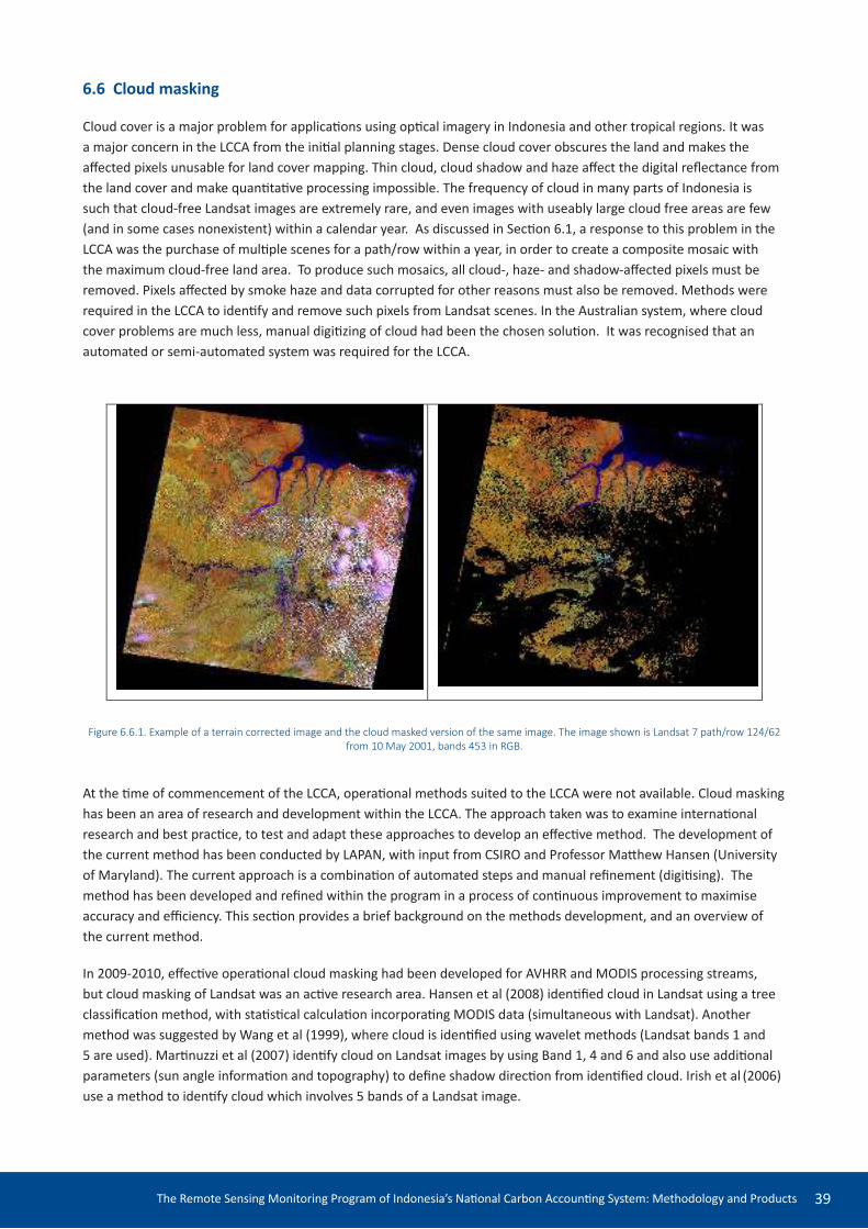
The Remote Sensing Monitoring Program of Indonesia’s Naional Carbon Accouning System: Methodology and Products 39
6.6 Cloud masking
Cloud cover is a major problem for applicaions using opical imagery in Indonesia and other tropical regions. It was a major concern in the LCCA from the iniial planning stages. Dense cloud cover obscures the land and makes the afected pixels unusable for land cover mapping. Thin cloud, cloud shadow and haze afect the digital relectance from the land cover and make quanitaive processing impossible. The frequency of cloud in many parts of Indonesia is such that cloud-free Landsat images are extremely rare, and even images with useably large cloud free areas are few (and in some cases nonexistent) within a calendar year. As discussed in Secion 6.1, a response to this problem in the LCCA was the purchase of muliple scenes for a path/row within a year, in order to create a composite mosaic with the maximum cloud-free land area. To produce such mosaics, all cloud-, haze- and shadow-afected pixels must be removed. Pixels afected by smoke haze and data corrupted for other reasons must also be removed. Methods were required in the LCCA to idenify and remove such pixels from Landsat scenes. In the Australian system, where cloud cover problems are much less, manual digiizing of cloud had been the chosen soluion. It was recognised that an automated or semi-automated system was required for the LCCA.
Figure 6.6.1. Example of a terrain corrected image and the cloud masked version of the same image. The image shown is Landsat 7 path/row 124/62 from 10 May 2001, bands 453 in RGB.
At the ime of commencement of the LCCA, operaional methods suited to the LCCA were not available. Cloud masking has been an area of research and development within the LCCA. The approach taken was to examine internaional research and best pracice, to test and adapt these approaches to develop an efecive method. The development of the current method has been conducted by LAPAN, with input from CSIRO and Professor Mathew Hansen (University of Maryland). The current approach is a combinaion of automated steps and manual reinement (digiising). The method has been developed and reined within the program in a process of coninuous improvement to maximise accuracy and eiciency. This secion provides a brief background on the methods development, and an overview of the current method.
In 2009-2010, efecive operaional cloud masking had been developed for AVHRR and MODIS processing streams, but cloud masking of Landsat was an acive research area. Hansen et al (2008) ideniied cloud in Landsat using a tree classiicaion method, with staisical calculaion incorporaing MODIS data (simultaneous with Landsat). Another method was suggested by Wang et al (1999), where cloud is ideniied using wavelet methods (Landsat bands 1 and 5 are used). Marinuzzi et al (2007) idenify cloud on Landsat images by using Band 1, 4 and 6 and also use addiional parameters (sun angle informaion and topography) to deine shadow direcion from ideniied cloud. Irish et al (2006) use a method to idenify cloud which involves 5 bands of a Landsat image.

The Remote Sensing Monitoring Program of Indonesia’s Naional Carbon Accouning System: Methodology and Products40
In terms of operaing internaional systems at that ime, Professor Mathew Hansen (then at South Dakota State University (SDSU)) was developing an automated tree-based cloud masking step within a Landsat ime series processing stream, and was a collaboraive partner in the INCAS-LCCA. His method was semi-supervised, involving the generaion of trees from training data where each branch of the tree was a split on a spectral index and threshold. Eventually by these successive index-threshold splits, each pixel was classiied as cloud-afected or not. The result was a cloud mask for the image. At SDSU, the index-threshold rules determined from training data were ixed and applied to calibrated imagery within a processing stream. In December 2010, through the INCAS collaboraion, Hansen provided a training course at LAPAN in this tree-based approach, and how to train and implement it in commercial sotware package. In pracice, the method proved diicult to implement in the LCCA; results (the masks from decision trees) from diferent operators proved highly variable. When trees derived from one set of images were applied to other images the results were oten unsaisfactory. In the SDSU system, a common tree is derived from training on very numerous Landsat images. SDSU assisted further by applying their own sotware in the US to a sample of 25 LCCA terrain-corrected images. The results worked well in many but not all situaions of cloud, shadow and land cover in Indonesia, and it was diicult to apply improvements directly to the results. This experience provided valuable learnings to the LCCA; in paricular idenifying the thermal band as important for detecion of thin high cloud and also providing experience in applying indices and thresholds to the problem.
In response to these problems, LAPAN commenced development of a method which combines rules from spectral indices and angular informaion to produce a cloud mask. The development commenced with tesing of indices and thresholds to idenify cloud, haze and shadow from clear land cover using staisical methods. A combinaion of index-threshold rules were ideniied, thresholds selected and applied to images, and the results evaluated. This process ideniied cloud/shadow and land cover combinaions where cloud masking was diicult, and those which were efecively masked by diferent indices. Land cover types which were erroneously masked (commission errors) were also ideniied. These indings were used to iterate the analysis process and to idenify new, potenially more efecive indices.
In general, it was found that bright clouds were efecively masked by brightness ‘albedo’ indices but that thresholds which ideniied all such cloud typically resulted in errors of commision by masking areas of bright land cover (such as roads or bare dry land). Cloud shadow areas are ‘dark’, but variable according to cloud density and land cover; masking such areas usually resulted in commission errors (over-masking) of ‘dark’ land covers such as dark forest or irrigated rice ields. Clouds and their shadows are of course linked and the locaion of one can be predicted from the other if the solar posiion and cloud height are known. This informaion was used to remove many errors of commission by using solar angle informaion (extracted from the satellite metadata), and esimates for the range of pixel displacement between a cloud and its shadow (arising from cloud height) derived from numerous images in Indonesia. The albedo values for smaller or thinner clouds or near the edges of thick cloud tend to overlap those for some ground covers. ‘Possible’ cloud is ideniied by a second, lower albedo threshold. Such areas are added to the mask if they are ‘close’ to the bright clouds or ‘paired’ with a shadow feature. The logical rules to implement this reinement may be described as follows:
1. Bright pixels are classiied as ‘cloud’ using an albedo index-threshold rule; thresholds are chosen (‘certain’ and ‘possible’) to classify all visible cloud. Bare land is excluded from these pixels using another index-threshold rule. A threshold applied to the thermal image band is chosen to classify thin cloud as ‘certain’ cloud.
2. Dark pixels are classiied as ‘shadow’ with water excluded using index rules, similarly.
3. Angular reinement. The regions found in (1) and (2) are ‘grown’ by a bufer within the program to include possible thin cloud/shadow and mixed pixels and to allow for varying cloud heights. The relaionship between a cloud pixel and its shadow is calculated from sun angles as a displacement in number of pixels in x and y direcions.
(a) From pixels classiied as ‘possible cloud’, the posiion of corresponding shadow is predicted, if these pixels are not classiied as ‘shadow’ in (2), the cloud classiicaion is assumed to be an error and removed.

The Remote Sensing Monitoring Program of Indonesia’s Naional Carbon Accouning System: Methodology and Products 41
(b) From pixels classiied as ‘shadow’, the posiion of corresponding cloud is predicted, if these pixels are not classiied as cloud in (1), the shadow classiicaion is assumed to be an error and removed.
[Allowance for missing matches near image borders is made in this step; it is also noted that the missing data from LS-7 SLC-of images afects this part of the algorithm as matching pixels for cloud or shadow may be missing.]
4. Filling; small gaps within and between cloud and shadow regions are illed. Fixed thresholds deine ‘small’.
5. Remaining classiied pixels are ‘grown’ by a bufer to ensure mixed pixels are included. The default bufer ‘grow distance’ is 3 pixels.
The rules are implemented in a single sotware program. In the iniial development and tesing of the approach, operators were required to set thresholds manually for each image, using interpretaion on screen to classify cloud and shadow; the angular reinement correcion was then run. With experience, default thresholds were ideniied, used as staring values and found oten to be efecive. Now three sets of default thresholds for the indices have been recorded. A program is run which automaically produces three versions of the automated mask. The operator selects the best for subsequent steps – or if none are saisfactory, is required to reset thresholds manually.
Following this processing, the resuling cloud and shadow masks are examined visually and a manual digiising step is typically carried out to remove any remaining unmasked bad data (most oten haze); or to idenify any large areas of commission. The results of the digiising and original masks are combined and then used to relabel pixels in a masked copy of the image using supplied programs.
The processing steps are described and illustrated below.
Step 1: Run a batch script that uses the cloud masking program (LPNcloudshadow_v8). Input data iles are (1) the terrain corrected Landsat image (2) a text ile generated at earlier steps which contains solar posiion informaion (3) the default thresholds sets. The outputs are separate cloud and shadow mask iles; these are single band raster classiicaion iles. Three sets are iniially produced using the default parameters; only the best is kept.
The index formulas used are as follows:
(a) To idenify bright cloud, two indices are combined, a simple brightness and a second index which helps to retain bright bare ground areas
B1+B2+B3)/3 >Ta1,Ta2 and (2*B1-B2-B3+2*B4-2*B7) > Tb
Where B1...B7 are the digital numbers for the Landsat bands, Ta1 , Ta2 and T
b are certain and possible
thresholds for the albedo and bare land indices respecively
(b) To idenify high cold cirrus cloud, which may be thin and omited by (a) above, a simple threshold (Tc ) is
applied to the Landsat thermal band
B6 < Tc
(c) To idenify shadow (dark) two indices are used in combinaion. The second index helps to separate water from shadow
(B4+B5)/2 < Ts) and (B2+B3-B5) < T
w
Ts
and Tw
are referred to as the shadow threshold and the ‘water’ threshold respecively

The Remote Sensing Monitoring Program of Indonesia’s Naional Carbon Accouning System: Methodology and Products42
As noted above, sets of default thresholds have been deined for this step. They can be seen below with angular informaion from a paricular image.
_def1 _def2 _def3
Table 6.6.1. Default threshold coeicient sets used in running the cloud masking program
The ‘best’ thresholds are not necessarily the ones that produce the most accurate masks. They are the ones that produce a result that can be corrected with the least amount of manual digiising efort. For example, small scatered clouds are very ime consuming to digiise so it is beter to set the thresholds to mask all such cloud and perhaps ‘over-mask’ roads or recently cleared land where these can be corrected with a few large polygons. Similarly, a large area of thin haze may be omited from the automaic mask to prevent over masking of agricultural lands because it can be digiised with a single polygon.

The Remote Sensing Monitoring Program of Indonesia’s Naional Carbon Accouning System: Methodology and Products 43
Examples of thresholding seing for the components of the cloud and shadow masking indices are shown in igures below.
Image L5_116059_090606 Brightness index mask (red) with a threshold (Ta1) of
45
Image L5_116059_090606 Brightness index mask (red) with a threshold (Ta1) of
40
Image L5_116059_090606
Brightness index mask (red) with a threshold (Ta1) of
30
Image L5_122059_090807 original Brightness index mask (red) with a threshold (Ta1) of
25
Figure 6.6.2. Paired input images (let) and masked brightness index (right) in red produced using the indicated brightness threshold. Bands 453 in RGB.

The Remote Sensing Monitoring Program of Indonesia’s Naional Carbon Accouning System: Methodology and Products44
In Figure 6.6.2, it can be seen that haze in the second image may not be completely masked, while in the upper right of the two lower images some ‘over-masking’ of bright land as cloud (errors of commission) are apparent. In the botom image this occurs in a cloud-free area and can be quickly corrected with manual digiizing at the next stage.
Image L5_116059_090606 Thermal mask (yellow) with a threshold (Tc) of 115
Figure 6.6.3. Paired input images (let) and masked thermal index (right) in yellow produced using the thermal image only.
Bands 453 in RGB
Figure 6.6.4 Paired input images (let) and masked shadow index (right) in pink produced using the indicated brightness threshold. Bands 453 in RGB
Figure 6.6.5. Further example of an image and its masked shadow index showing the efect of varying the threshold. The mask is covering dark areas associated with terrain which have remained ater terrain correcion; adjusing the threshold removes most of this error while sill masking the true
shadow. Bands 453 in RGB.
L5_116059_090606 Shadow mask (pink) with a threshold (Ts) of 55
Image L5_116059_090606 Shadow mask (pink) with a
threshold (Ts) of 55
Shadow mask (pink) with a
threshold (Ts) of 45

The Remote Sensing Monitoring Program of Indonesia’s Naional Carbon Accouning System: Methodology and Products 45
Step 2. Operator must review the results by visual inspecion. A good set of threshold-derived masks will cover all visible cloud and shadow with minimal commission error, or with errors which can be easily digiised and corrected in the subsequent steps. Errors such as shown in Figure 6.6.5 (centre) will indicate that revision of thresholds is required, and the operator will be required to perform manual threshold adjustment.
Step 3. Digiising to edit the cloud and shadow masks. The operator must check for errors of omission and commission. Vector outlines are digiised manually to add areas to the mask and delete errors of commission; the vectors are known as the ‘add’ and ‘delete’ vectors. All omission errors (bad data which remains ater masking) are important and must be removed. It is desirable to remove commission errors as they represent masked good data which otherwise will not be used. Typical errors of omission will be thin haze and shadow; oten these afect large coniguous areas and can be digiised quickly. Causes of commission errors are various, relaing to land cover as well as cloud and shadow signatures, and may occur as many small areas. Where commission errors occur in cloud-free regions (Figure 6.6.2), they can be corrected easily. Where commission errors occur as small patches within patches of true cloud and shadow, the digiising efort may be considered too great. An example is shown below.
Original Image L7_120066_290612. This is an LS-7
SLC-off image. Only land is at top right.
The masked image image before editing
Detail of above: area indicated by the red rectangle
above
Detail of above; same area as at left
Figure 6.6.6. Example. Input image and outputs from the automated cloud masking program prior to ediing. Bands 453 in RGB.

The Remote Sensing Monitoring Program of Indonesia’s Naional Carbon Accouning System: Methodology and Products46
Figure 6.6.7. Example of manual digiising correcion of cloud masks. Input image and outputs from the automated cloud masking program together with manual edits (vectors). Bands 453 in RGB.
Further detail of original Image
L7_120066_290612
Cloudmasked image for same area as at left. Yellow
lines indicate digitised cloud areas to be added to
the cloud mask
Detail of original image showing digitised
commission errors which are deleted from the
mask.
Same area and same vectors as at left on the maked
image from thresholded masking program
Step 4. Combining masks and creaion of the inal masked image for QA is done by running a program; the inputs are the terrain-corrected image, selected mask raster iles and the two ‘add’ and ‘delete’ vector iles. The output is the masked image, and new ‘inal mask’ iles produced from modifying the input masks with the vector deleions and addiions. Creaing inal raster masks allows them to be applied to other versions of the image, for example to mask the BRDF-corrected image.
QA for cloud masking is conducted by an independent experienced operator who essenially begins at step 2 above, examing the image, the vectors, and the cloud masked image. Experienced operators can readily detect whether any problems are likely to be ixed by revising the thresholds for cloud or shadow. In such cases, the image will fail and the operator should be advised of the suggested changes to be tried. If the threshold classiicaion appears adequate, and some errors remain, then vector ediing is required. Any unmasked cloud or shadow data requires correcion; and ‘overmasking’ will be assessed and, if signiicant and correcible with reasonable efort, the vector ile must be revised. Revisions to the vectors are usually performed by the QA operator.

The Remote Sensing Monitoring Program of Indonesia’s Naional Carbon Accouning System: Methodology and Products 47
6.7 Mosaicing
The mosaic process produces a composite of all LCCA images within a ixed spaial extent for each year of LCCA coverage. These mosaic units form the basis for subsequent processing and products. Mosaicing can start when cloud masking of all LCCA images within the mosaic area for a year is completed. Within the mosaic process, muliple cloud-masked images within each path/row for that year are composited. The result is a single image, the ‘mosaic image’ for that year, covering the speciied extents with minimum missing data. Only the six muli-spectral image bands are in the mosaic. The thermal image band is not retained ater cloud masking is complete.
The mosaic extents are deined in NUTM projecion. They have been modiied from standard UTM map zones in order to include complete islands or island groups of Indonesia as far as possible. They are referred to as INCAS-LCCA mosaic iles, and named for the standard map zone with greatest area within the mosaic. There are 13 standard LCCA mosaic iles covering Indonesia (Figure 6.7.1).
Figure 6.7.1: LCCA mosaic iles for Indonesia
As with the individual images, all mosaics within the LCCA are referenced to NUTM coordinates (WGS84 datum). If conversion to SUTM is required for any reason, only a simple constant shit (or ofset) in northing is required. Table 6.7.1 lists the extents of the standard LCCA mosaics in NUTM coordinates. These extents include an overlap with adjacent mosaic iles. The ile size for each mosaic ile as a six-band Landsat mosaic is very large. For convenience in storage and processing, each mosaic ile is divided further into standard ‘quadrants’ with a maximum ile size of 2Gb (named e.g. 48C_nw for the northwest quadrant within mosaic ile 48C). The names and extents of these quadrants are found in the Operaional Manual.

The Remote Sensing Monitoring Program of Indonesia’s Naional Carbon Accouning System: Methodology and Products48
Table 6.7.1 . The extent of LCCA Mosaic Tiles; coordinates are all deined in WGS84, NUTM projecion in the zone number indicated by mosaic name
Descripion Map Sheet ID Top Let Botom Right
Sumatra NW 47N 0, 750 000 950 000, -100 000Sumatra SW 47S 300 000, 50 000 950 000, -600 000Sumatra E 48C 100 000, 415 000 930 000, -750 000Kalimantan W 49N 50 000, 550 000 930 000, -500 000Java 49S -210 000, -530 000 960 000, -1 000 000Kalimantan E 50N 90 000, 550 000 800 000, -560 000Nusa Tenggara W 50S 150 000, -450000 800 000, -1 100 000Sulawesi 51N -40 000, 280 000 875 000, -790 000Nusa Tenggara E 51S -10 000, -675 000 1 000 000, -1 250 000Maluku N 52N -100 000, 621 000 780 000, -350 000Maluku S 52S 75 000, -250 000 920 000, -1 000 000Papua W 53C -100 000, 50 000 760 000, -840 000Papua C 54C -30 000, -110 000 580 000, -1 100 000
The creaion of the mosaics proceeds as follows.
First, all of the cloud masked images within the mosaic extents from the chosen year are assembled. The majority will have been reciied to the required projecion for that zone. Edge images and images in overlap areas which require reprojecion are ideniied, and are reprojected using cubic convoluion resampling. The operator will display all images from the same path/row and perform a visual assessment, with paricular atenion to any visual edge efects within an image and comparison of the locaion of clear areas. If any areas of data within a scene are judged to be poor quality for any reason, a simple vector is drawn and a program is run to mask these areas. The most common cause for this is subtle haze efects which are not detected in the masking step that are observed when observing data from the same area on two or more dates. Areas of scatered clear data where another image has complete clear data may also be manually excluded from the mosaic by this process. Low resoluion ‘snapshot pictures’ are created from each image to allow faster comparison of images and the creaion simple simulated mosaics.
The next step in mosaicing is to determine a priority order for mosaicing of images over the whole ile. Within path overlaps and where muliple images are available within a path/row, choices are made about the data from image is retained in the mosaic. The purpose of this process is to produce the best possible mosaic for subsequent numerical processing in the LCCA. The output from this step is a ‘mosaic order’ list which speciies which images are to be mosaiced on top of others. Data pixels from higher scenes will be used, but any missing data pixels in these will be illed from lower order scenes in the list where such data exists. The result is a composite mosaic for the year with minimal missing data – remaining areas of missing data will be those for which no good data exists in that year ater the image selecion and processing steps described above.
A set of rules to determine the overlay order has been deined. The consideraions include:
a) haze-free, dry images are preferred over cloudy or green images or images with other issues;
b) images with large unmasked data areas are selected above images with small areas of data, but...
c) images with coniguous clear areas (perhaps only in a porion of a whole image) may be selected above images with scatered missing data throughout;
d) LS-7 SLC-on images are preferred over LS-5
e) LS-5 images are preferred to LS-7 SLC-of images

The Remote Sensing Monitoring Program of Indonesia’s Naional Carbon Accouning System: Methodology and Products 49
The result of these decisions is the ‘mosaic order list ile’ - which is a list of input images (cloud masked scenes) in mosaic order for the mosaic ile. This overlay order is copied for overlapping mosaic iles so that the overlay order is consistent across the whole country within each calendar year.
The inal step is to create the mosaic itself, by running the mosaicing program. The inputs to the program are the masked images and the order list ile. Two output iles are produced: the six-band mosaic for the ile in four or six ‘quadrant’ pieces depending on ile sizes; and a two-band ‘mosaic-date’ image of the same dimension which records for each pixel the date and path/row of the source image from which its data has come. Even ater using all available images, typical mosaics will sill contain some missing data due to cloud. The results of the mosaic process for Sumatra in 2008, the mosaic image and raster mosaic dates image, can be seen in Figure 6.7.2. Figure 6.7.3 shows the mosaic for Java for 2008.
(a)
(b)
Figure 6.7.2. (a) Mosaic of Sumatra in 2008 (combined from 47N, 47C and 48C mosaic iles); bands 453 in RGB. (b) Mosaic date informaion displayed in colour (the example pixel values indicate the source was from path/row image 130/57 acquired on 31 May 2008).
Figure 6.7.3. Display of mosaic Landsat Image for Java in 2008 (mosaic ile 49S); bands 453 in RGB, black areas over land indicate missing data for that year.

The Remote Sensing Monitoring Program of Indonesia’s Naional Carbon Accouning System: Methodology and Products50
Mosaicing QA is performed by the QA team. The QA process involves irst checking the completeness of the data ile and the overlap order ile of image dates. The next stage is to check visually the Landsat image mosaic by displaying the result of mosaic along with the date image mosaic. The inal mosaic is compared to the simulated mosaic from the ‘snapshot’ pictures to ensure that no data has been omited or incorrectly located. Adjoining quadrants are compared with each other and with adjoining mosaic iles that are already complete to ensure the same overlay order in the overlaps. The QA team may reject and return to operator if any problems are detected. Provided all available scenes have been used, QA may suggest a change in order of mosaic, or removal (masking) of speciic problem areas from an input image.
Once the mosaic has passed QA, it will be archived for use as an input for the next stages. Terrain-corrected mosaic images have already been produced for all of Indonesia for each year from 2000 to 2009. Mosaics for 2010 to 2012 will be complete in the middle of 2014. These are archived at LAPAN.
The frequency of cloud-free data can also be summarised. The missing data in mosaics over the 13 years can be used to esimate and illustrate the frequency of cloud problems within a year for data in various areas within the LCCA processing region. The data may also be summarised year by year to provide the proporion or area of cloud free data for each island group. In combinaion with summaries of the numbers of input images, these data might be used to predict the proporion of cloud-free imagery if full archives are available (as will be the case with LS-8) and if more frequent opical data were available.
Figures 6.7.4 and 6.7.5 show spaial summaries of the amount of clear land in the ten years from 2000 to 2009. Table 6.7.2 shows area summaries. Each pixel is coloured according to the number of years in which there was clear data suitable for forest mapping. Shades of green indicate pixels with data in all or most of the 10 years. Shades of blue indicate pixels with data in around half of the 10 years. Shades of yellow (3), orange (2), pink (1) and red (0) indicate pixels with data in few of the 10 years. Not surprisingly, the drier regions of Indonesia have clear data in more years. Some of the mountainous areas have the least data available. In parts of Papua, this may be the result of over-masking of snow and ice. The Riau and Jambi provinces in Sumatra also show low data coverage, most likely due to smoke haze. Such summaries can be used to prioriise searches for alternaive data sources. For example, due to alitude and/or slope consideraions broad scale land use change is unlikely in mountainous regions and so may be a low priority.
10 9 8 7 6 5
4 3 2 1 0
Figure 6.7.4. Display of the number of years from 2000 to 2009 with data suitable for forest mapping for the whole of Indonesia. As shown in the legend, shades of green indicate that there is clear data in most years; shades of blue indicate that there is clear data in around half the years; shades
of yellow, orange and red indicate clear data in only a few years.

The Remote Sensing Monitoring Program of Indonesia’s Naional Carbon Accouning System: Methodology and Products 51
Figure 6.7.5. Display of the number of years from 2000 to 2009 with data suitable for forest mapping for sample regions in more detail. As shown in the legend in Figure 6.7.4, shades of green indicate that there is clear data in most years; shades of blue indicate that there is clear data in around half
the years; shades of yellow, orange and red indicate clear data in only a few years.
Table 6.7.2 . Percentage land area with equal to or greater than ‘years of clear data’ data density by region
Years
of Clear Data
Whole of Indonesia
Sumatra Kalimantan Java SulawesiNusa
TenggaraMaluku Papua
1 98.44 99.81 99.34 99.99 99.22 99.99 99.36 94.552 95.85 99.17 97.30 99.95 96.44 99.97 97.62 87.813 91.33 97.32 92.54 99.72 91.60 99.867 94.20 78.46
4 84.16 93.05 83.72 99.08 84.71 99.51 88.09 66.65
5 74.30 85.87 70.71 97.54 75.69 98.70 78.42 53.286 62.24 75.67 54.81 94.33 64.13 97.11 65.28 39.397 48.80 62.16 38.40 89.24 49.97 94.11 49.60 26.018 35.54 46.82 23.93 81.87 34.32 89.44 33.05 14.759 23.21 30.30 12.59 70.07 19.10 81.32 18.14 6.51
10 10.94 12.03 4.28 42.90 6.15 63.848 6.82 1.50
The current LCCA mosaics produced from the terrain corrected and cloud-masked data are the inputs to forest mapping processes. Using the mosaic list ile and data archived at LAPAN it is also possible to produce mosaic products using the BRDF-corrected imagery prior to terrain correcion as inputs. These mosaics may be preferred for some purposes including visual interpretaion.

The Remote Sensing Monitoring Program of Indonesia’s Naional Carbon Accouning System: Methodology and Products52

The Remote Sensing Monitoring Program of Indonesia’s Naional Carbon Accouning System: Methodology and Products 53
7. DETAILED METHODOLOGY - FOREST EXTENT AND CHANGE MAPPING
This secion describes the LCCA processing methods to produce the forest extent maps from all years of the mosaiced data. Three major stages are described. The irst stage is the creaion of a ‘forest base’ probability image for a chosen single year. In this stage, a ‘irst’ forest probability map is created using supervised classiicaion methods applied to the LCCA mosaics for that year. The process requires expert input to advise on land cover, and applicaion of staisical procedures to derive the classiied forest probability map. Operator judgment is used to evaluate and reine threshold parameters in the image classiicaion process. The staisical procedures are essenially mulivariate discriminate analyses; in paricular canonical variate analysis (CVA) and related procedures. CVA is described in Campbell and Atchley 1981; and further described in applicaions using image data in Cacceta et al 2007, Furby et al 2010. In the second stage of processing, referred to as ‘Matching’, this base probability image is then the input to a semi-automated classiicaion which produces forest probability images for the remaining years in the ime series. In the third stage, these single-date forest probability images are then combined using a fully automated muli-temporal classiicaion model to produce reined forest probability maps for each year. The mathemaical framework for this process is known as a condiional probability network (CPN) (Lauritzen 1992, Lauritzen & Spiegelhalter 1988). Development and applicaion of CPNs to land and forest monitoring is described in Kiiveri & Cacceta (1998) and Kiiveri et al (2001, 2003). Furby (2002) describes in detail the applicaion of CVA and CPN within Australia’s forest monitoring system.
Numerous methods exist for image classiicaion. In the LCCA, a simple index and threshold image classiicaion methodology is used to produce the single-date probability images. The approach is opimised locally for diferent vegetaion and land use communiies at the base mapping stage, through applicaion of CVA and related rouines. One advantage of this approach is that the methodology is much more easily understood and adjusted to local circumstances by the operators at the base mapping stage. A second advantage of this approach is that it can be applied through the matching process to other years in the automated matching process. This is both eicient and criically important in maintaining consistency over ime. Temporal consistency is a paramount consideraion in a monitoring system of this kind; within the LCCA, temporal consistency is further improved by the muli-temporal processing stage. It has been shown that, once combined with the muli-temporal processing model in the third stage, the index-threshold classiier used in the irst and second stages provide results as accurate as applying far more complex iniial classiicaion methodologies (O’Connell and Cacceta 2009).
7.1 Forest base mapping
The base mapping uses a combinaion of data inputs and knowledge to guide and tune the local classiicaions (see Secions 5, 6.2). Experts with knowledge of ground cover in the region provided criical inputs through interpretaion of high resoluion images and Landsat mosaics, supported by maps and ground photographs where available. The base mapping process for each region was conducted as a dedicated workshop typically over three weeks, where image processing and staisical experts worked closely with the regional experts in an integrated team. The forest base workshop is a manually intensive process, but is carried out only once for each region to create the base. For adding other years to an exising ime series, only the second and third stages, which are semi and fully automated, need be performed.
The irst step in forest base mapping is to select the ‘base year’ for the process. In the LCCA, at least three years of mosaics were required to be completed prior to the base mapping; typically mosaics for 2008, 2006 and an earlier year (2000 or 2001) were available. Year 2008 was generally the desired choice as it was close in date to most of the high resoluion images. Further, as the most recent available mosaic, it was most relevant to recent experience and

The Remote Sensing Monitoring Program of Indonesia’s Naional Carbon Accouning System: Methodology and Products54
memory of the ground experts. Missing data in mosaics was however an important consideraion, as it is desirable that the base mapping be as complete as possible. Where cloud cover was signiicant, an alternaive base year was chosen, someimes only for sub-regions in the mosaic.
There are three main steps in creaing a base forest probability image:
1. Dividing the region into straiicaions zones. The forest base analysis and classiicaion are carried out separately within each straiicaion zone.
2. Deriving indices to discriminate between forest and non-forest cover for each straiicaion zone. This process applies staisical analyses to training samples covering the range of forest and non-forest covers within the zone.
3. Seing thresholds for these indices that in combinaion idenify certain forest cover, certain non-forest cover and the uncertain spectral region for each straiicaion zone for the base year. Diferent thresholds may be used for some image dates within the base year mosaic.
Each of these steps will be discussed in more detail below.
7.1.1 Straiicaion.
The land use and land cover (including forest and non-forest vegetaion) varies greatly across Indonesia – from the drier tropical savannas in Nusa Tenggara to the wet peat forest of Sumatra and Kalimantan and the high alitude vegetaion in Papua. A single image classiier cannot successfully separate all these diferent land cover types simultaneously. Instead, the approach adopted in the LCCA is to subdivide (or straify) the whole area into smaller regions (zones) within which the mix of land covers and land uses are much simpler. The classiier can then be directed (by analysis) to separate the forest and non-forest cover types which occur within that region; e.g. dryland forest and dryland non-forest land uses, or coconut palms from mangrove and wetland forests, or rice crops from wetland forest.
Figure 7.1.1 shows the straiicaion zones for Kalimantan. The light orange ‘background’ colour shows the central mountainous dryland forest straiicaion zone. The darker orange zone at the botom right was wetland forest in the 1990s which was cleared for agriculture as part of the larger ‘transmigraion’ area on Kalimantan. Litle natural forest remains in this zone. The red area next to it is predominantly the original wetland forest with only small patches of agriculture and setlements. The small purple zones next to the dark orange zone are regions of rubber plantaions. Rubber is very diferent in the images to other forest plantaions. The colours in the satellite image on the right of Figure 7.1.1 look quite diferent between these four zones and so it logical to treat them separately in the forest mapping process.
Figure 7.1.1. LCCA inal straiicaions zones for Kalimantan (let) and a zoomed-in display of the boundaries overlayed on the 2008 Landsat TM mosaic image (bands 5, 4, 3 in RGB) on the right.

The Remote Sensing Monitoring Program of Indonesia’s Naional Carbon Accouning System: Methodology and Products 55
Soil, climate, terrain and geology feature prominently in the factors that cause regional diferences in land cover and land use. Access to datasets or expert knowledge of these can assist in the straiicaion process. Broad variaions in vegetaion spectral response and agricultural land use can be ideniied iniially from inspecion of the image mosaics. Regional experts with knowledge of land use and forest types provide criical input to the straiicaion of a region. Straiicaion zones are iteraively reined within a base workshop. Analysis of training sites from within the zones and review of iniial forest mapping (described below) may suggest addiion of further straiicaion zones or changes in boundaries to improve the accuracy of the forest maps. The inal straiicaion zones, as vector and raster maps, are the archived outputs of this step.
7.1.2 Deriving indices for separaing forest and non-forest cover
Indices - linear combinaions of the Landsat image bands for separaing forest and non-forest land covers - are opimised locally for each straiicaion zone. The index derivaion process is driven by ground truth informaion – sample areas of forest and non-forest vegetaion cover are selected from the image mosaic of the base year using ground truth informaion. Comprehensive samples of forest and non-forest cover are required within each straiicaion zone. Ground truth data includes high resoluion satellite imagery (1-2m resoluion) in which tree and non-tree cover is evident (Figure 7.1.2). Local experts who have a deep familiarity with the region and its land cover are criical. Based their knowledge, and viewing the high resoluion data along with Landsat mosaics, interpretaions of land cover are extrapolated spaially. These sample areas are indeniied in the Landsat image mosaic as training site polygons and labeled. The analyses are directed towards discriminaing between the paricular training sites used. Provided that the sites are representaive of the cover in the images, the indices and thresholds that separate the training sites will separate all forest and non-forest cover in that zone.
Figure 7.1.2. Landsat TM satellite image (let) with bands 4, 5, 3 in RGB and a high resoluion image of the same area. The yellow outlines show forest and not forest training samples (sites) ideniied in each image.
As noted above, the image year selected for the forest base analyses is typically the one closest in date to most of the ground truth imagery and as close to the present as possible, to relate best to the memory of the local experts. One or two other image years may be included in these index derivaion analyses so as to represent the seasonal variaion in the ime series. The advantages of including the extra images in the iniial processing are that indices are found that work over a range of years, not just opimised for the condiions present in any paricular year, or the need to account for variaions in condiions between years is established very early in the process.

The Remote Sensing Monitoring Program of Indonesia’s Naional Carbon Accouning System: Methodology and Products56
Staisical analyses are applied to idenify the required spectral indices. Canonical variate analyses are performed using the training data to derive suitable indices for discriminaing between forest and non-forest cover. A CVA inds the linear combinaions of the image bands that maximise the diferences between training sites relaive to the variaion within the sites. The canonical vectors give the direcions of maximum site separability and the canonical roots give a measure of the amount of site separaion in these direcions. The canonical vectors, which are linear combinaions of image bands, form the basis of the indices to be used. The usual canonical variate analysis will ind the canonical vectors that best separate each of the training sites from every other training site. The canonical variate analysis can be modiied to focus on the separaion of paricular groups of reference sites (forest and non-forest) rather than between all the sites. This is done using contrast vectors to focus on supplied groupings of the reference sites.
Index Coefficients Proportion of
Separation Provided
Image A
Proportion of
Separation Provided
Image B
-0.035 0.34 -0.068 -0.078 100% -
-4 34 -7 -8 99.92% -
-1 8 -2 –2 99.25% -
0 4 -1 –1 99.34% 74.22%
0 1 0 0 74.10% 97.58%
-0.068 0.26 0.013 0.003 - 100%
-7 26 1 0 - 99.96%
-1 3 0 0 75.28% 99.29%
-1 4 -1 -1 96.61% 65.59%
-1 4 1 1 38.15% 92.38%
-1 4 0 0 75.37% 99.74%
-1 5 0 0 75.27% 99.67%
0 3 -1 –1 92.29% 55.50%
0 5 -1 –1 99.25% 83.24%
0 6 -1 –1 97.34% 87.99%
0 7 -1 –1 95.17% 90.74%
0 8 -1 –1 93.17% 92.45%
Figure 7.1.3. Top let: Sample canonical variate means plot. Site that are ploted close together are spectrally similar and sites are ploted further apart are more separable. The dashed lines separate most of the forest sites from most of the non-forest sites. Top Right: Contrast groups to derive
indices for the lines of best separaion. Botom Let: Table showing index smoothing for robustness through ime. Botom Right: Resuling index plot.

The Remote Sensing Monitoring Program of Indonesia’s Naional Carbon Accouning System: Methodology and Products 57
The canonical vectors found by this process relate speciically to the paricular training sites and image dates used in the analyses. The vectors are simpliied, or smoothed, to make them more robust over the range of cover types and image dates. In this process, smoothed vectors, or indices, are sought that perform well over all of the selected representaive image dates. Informaion staisics allow alternaive indices to be compared. Figure 7.1.3 summarises outputs from the CVA and index-smoothing rouines. This process can also be used to compare global vegetaion indices (e.g. NDVI) as well as indices from similar straiicaion zones (Figure 7.1.4).
As well as producing a paricular index or indices for separaing forest and non-forest cover, the analyses also provide an objecive measure of the number of indices required for adequate discriminaion. The analyses have shown that for Landsat TM images the majority of the separaion is obtained with a single index. However, a second masking index is always required to separate paricular problemaic cover types. Occasionally three indices are required.
It is noted here, and expanded below, that perfect separaion is rarely provided by the indices for all pixels. The analysis indicates index values where classiicaion is ‘uncertain’ (Figure 7.1.4). This is relected in the classiicaion as probabiliies as discussed below.
Figure 7.1.4. Index Plots from global indices (NDVI and Landsat TM band 5) and smoothed locally opimal indices. The green box in each is the certain forest spectral region – it contains only forest training sites. Outside the blue box is the certain non-forest spectral region – it contains only non-forest
training sites. Between the two boxes is the uncertain spectral region – it contains both forest and non-forest training sites. The beter the indices separate forest and non-forest cover, the smaller the uncertain region will be. Here the local indices perform beter than the global indices.
7.1.3 Seing thresholds for separaing forest and non-forest cover
Having found appropriate indices to separate forest and non-forest cover for a zone, it remains to set thresholds for each year to allow pixels to be assigned probabiliies of forest (and non-forest) cover based on the values of the indices. These thresholds are set manually for the base year.
It will generally be the case that there is some spectral overlap between forest and non-forest training sites in each straiicaion zone, or at least a coninuum of index values. There will be a range of index values that correspond to pixels that can conidently be labelled as forest, (or conversely, couldn’t possibly be non-forest cover). There will also be a range of index values that correspond to pixels that can clearly be only non-forest cover. In between, there will also be a range of index values, where a pixel could be either forest or non-forest – a region of uncertainty. An example is shown in Figure 7.1.4. The green rectangle shows the certain forest region. The blue rectangle shows the combined certain forest and uncertain region. Outside the blue rectangle is the certain non-forest region.
As well as deining the edge of these three pariions of the image, the thresholds determine the probability assigned to each pixel. Pixels with index values in the certain forest spectral region are assigned a probability of forest cover of one (100%). Pixels with index values in the certain non-forest region are assigned a probability of forest cover of zero. Pixels with index values in the uncertain spectral region are assigned a probability of forest cover between

The Remote Sensing Monitoring Program of Indonesia’s Naional Carbon Accouning System: Methodology and Products58
Figure 7.1.5. Illustraion of threshold reinement from image displays which combine interpretaion of ground truth with classiicaion results(lower let). Thresholds are adjusted unil best results are achieved.
one and zero based on the closeness to the certain forest thresholds. The thresholds need to be set ensure that the probabiliies are high (or low) enough within the uncertain area. Iniial thresholds are set by inspecion of the index plots.
Reinement of the iniial esimates of the thresholds is conducted using image displays as in Figure 7.1.5. Operators assess whether there are cover types (image pixels) that are not adequately represented in the training data. This is an important process in which ground knowledge provides important input; operators may view, assess and discuss results of adjusing thresholds to minimise misclassiicaion and set appropriate probabiliies within the ‘uncertain’ zone. This assessment, by comparison of results from neighbouring zones, efecively opimizes use of ground truth over a wider area and may generate reinement of zone boundaries.
Yellow: p(forest) > 0Green = 0 excluded by index 1Red = 0 excluded by index 2
Index 1 + thresholds Index 2 + thresholds
Thresholds are set separately for each straiicaion zone, even if the same indices are applied to several straiicaion zones. It may also be necessary to locally adjust the thresholds for diferent image dates within a straiicaion zone, if the seasonal or atmospheric condiions are very diferent. Sub-zones are deined by intersecing the image date boundaries for the mosaic with the straiicaion zone boundaries.
When a saisfactory set of thresholds are obtained for a zone, it is saved and a forest probability image is created from this ile and the mosaic image, and reviewed. The forest cover probability images for the individual zones are overlaid as part of inal QA for the base. Zones and thresholds may be reined at this stage.

The Remote Sensing Monitoring Program of Indonesia’s Naional Carbon Accouning System: Methodology and Products 59
Within each zone, QA is essenially carried out by the team during this stage as a coninuous process by viewing alternaive results on screens, with reference to ground experts and to results from neighbouring zones. Examples of displays used in this process are shown in Figure 7.1.6. Beyond the areas of the LCCA high resoluion coverage, Google Earth(TM) is used in this assessment.
Landsat image
High resolution image
Forest probability
Landsat image
High resolution image
Forest probability
Figure 7.1.6. Two examples from Sulawesi for QA checking of classiicaion results. The base forest probability image is compared to Landsat image and high resoluion image. In these examples the high resoluion imagery is from Google Earth(TM)
The inal outputs from the base mapping are: a inal set of straiicaion zones in raster and vector format; a set of index-thresholds iles for each zone (and subzone); and the inal map of probabiliies for the region. QA is required to check these iles, the mosaic control program and the mosaic results. Examples of results are shown below.
Spectral separaion is impossible for some desired classes of forest (or non-forest) where the spectral signals overlap. In such cases other data or knowledge must be employed to correctly label such cover classes. An addiional process in the base mapping process and QA, which coninues in subsequent QA steps, is the ideniicaion of cover classes in diferent regions which result in errors in the forest probabiliies. Examples of problems of this type are:
• Some kinds of non-forest plantaion such as oil-palm - mature palms are ideniied as forest in probability image.
• Deciduous forest, e.g. cinnamon and teak forest, which may be incorrectly classiied depending on the season of imagery.
• Rice crops in some growing phases someimes have high probability and may be ideniied as forest.
• Fluctuaing water levels in wetlands create varying signals, some of which may be confused with forest.
In general, the locaion of these areas is restricted, and correcion approaches using other data may be employed – see Secion 8.

The Remote Sensing Monitoring Program of Indonesia’s Naional Carbon Accouning System: Methodology and Products60
7.1.4 Base mapping results: example
The results of the base mapping for Sulawesi, produced from base year 2008, are illustrated below. Figure 7.1.7 shows the mosaic and the straiicaion zones for the island. Figure 7.1.8 shows the base forest probability image. Figures 71.9, 7.1.10 and 7.1.11 show samples of the forest base map and high-resoluion imagery. Displays like these are used in the QA of the forest base probability image.
Figure 7.1.7. Sulawesi mosaic 2008 (let, bands 453 in RGB) and straiicaion zones (right)
Figure 7.1.8. Base forest probability image for Sulawesi. It is formed mostly from the 2008 Landsat mosaic with zone 6 from the 2006 Landsat mosaic. The red colour indicates probability calculated as 100% in base mapping; the blue colour indicates probability 0 (non-forest). Other colours indicate
the probability is between 0 and 100% as per the scale bar shown.
0
100

The Remote Sensing Monitoring Program of Indonesia’s Naional Carbon Accouning System: Methodology and Products 61
Figure 7.1.9. Example: Base forest extent (probability>50%) compared to high-resoluion imagery. Detail from Sulawesi.
Figure 7.1.10. Example: Base forest extent (probability>50%) compared to high-resoluion imagery. Detail from Sulawesi.
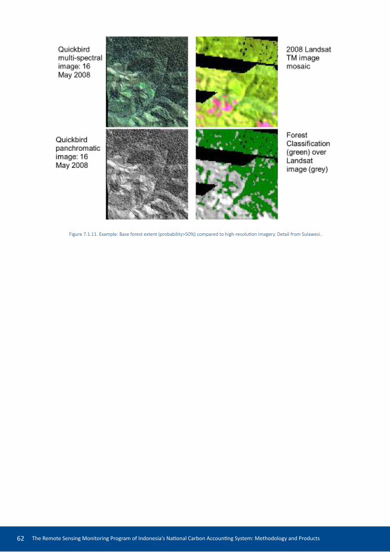
The Remote Sensing Monitoring Program of Indonesia’s Naional Carbon Accouning System: Methodology and Products62
Figure 7.1.11. Example: Base forest extent (probability>50%) compared to high-resoluion imagery. Detail from Sulawesi.

The Remote Sensing Monitoring Program of Indonesia’s Naional Carbon Accouning System: Methodology and Products 63
7.2 Matching: forest classiicaion for other years
Following the base mapping, a semi-automated matching process is applied to the LCCA mosaics to derive forest cover probabiliies for the other years. As described above, the indices used in the base mapping are developed by analysis; which typically considers more than one year. In the automated matching, it is assumed that the derived indices can be applied to their zone in all years – the matching process is run to set appropriate thresholds for each of the years, which can be applied to produce the classiicaion for that year. The matching process is applied in the Australian forest monitoring system (Cacceta et al. 2007, 2013); it has advantages of eiciency, of removing operator judgement and maintaining temporal consistency. Occasionally the automaion does not produce adequate results and some manual adjustment of thresholds is required.
This process requires as inputs the index-threshold iles for each zone, as well as the Landsat mosaic for the new year. The forest map probabiliies from an exising year are also required; iniially this is the base map as described above. Training regions are selected by operators for each zone, and within these regions the matching algorithm adjusts thresholds to produce a best match of probabiliies to the base using a criterion of minimum sum of absolute diferences. These matched thresholds allow probabiliies to be assigned to pixels to produce a forest probability map for the new date. Figure 7.2.1 illustrates this process.
Figure 7.2.1. Illustraion of the matching process. The top row shows the 2007 base year for a small region in Sulawesi and the same area in the 2009 image mosaic. A matching region is also shown by the yellow box. The two rows below show probability images on
the let. The let most probability image is for the 2007 base and is the same in both rows. The middle probability image is for the 2009 image. At the top, the probability image is calculated by applying the thresholds for the 2007 image. Below is the result of
adjusing the thresholds using the matching process. The image on the right in each row is the diference between the 2009 and 2007 probability image. Shades of green indicate litle diference between the two probability images. The remaining red and blue areas in
the botom row correspond to areas of change observed between the two Landsat image mosaics.

The Remote Sensing Monitoring Program of Indonesia’s Naional Carbon Accouning System: Methodology and Products64
The selecion of an exising date of probabiliies to which other years are matched is done by consideraions such as:
• In regions where a lot of land use change is expected between the images in the ime series, the ideal base image is one closest in ime to the ‘new’ image data so that there is the least change between the images being compared. We may prefer to match the 2009 imagery to a 2008 base, then 2010 to 2009. This is the strategy that was used for Kalimantan and Sumatra.
• In areas where the spectral change is mostly seasonal change in non-forest land use, a ixed (or common) base is preferred for overall consistency. All years would be matched to the irst forest base, 2008 say. This strategy was used for the remaining regions of Indonesia.
The QA team advises and may review the most suitable forest base probability image for each ‘new’ year.
Efecively, for the training ‘matching region’ and indices supplied, the matching program produces the best possible reproducion of the base probability image, according to the ‘minimum diference’ criterion. The program requires reasonable staring values of thresholds and these are provided from exising base thresholds iles for the zone. Thresholds are iteraively adjusted unil the best match (minimum sum of absolute diferences) is found.
Matching regions are selected for each zone. They need to be created by operators, and may produce varying results. In pracice, since the matching is automated, a number of regions for each zone are typically selected, and the best results chosen. Criteria for selecing matching regions to produce good results applicable to whole zone are as follows:
• they should be representaive of the whole sub-zone,
• contain suicient areas of forest and non-forest cover (in both the new and base image); and
• should not include a large proporion of areas of change in forest extent between the current and base years whenever possible.
Figure 7.2.2. Example of matching regions (rectangles) for zone 4 (red boundary) in Kalimantan overlaid on (a) base mosaic 2008 , and (b) mosaic from 2009. The yellow box is likely to be best because it include various types of land cover, others are dominated by a
reduced set of land cover such as mangrove, primary forest or areas outside the zone. Bands 453 in RGB.
An example of matching regions is shown in Figure 7.2.2.
(a)
(b)
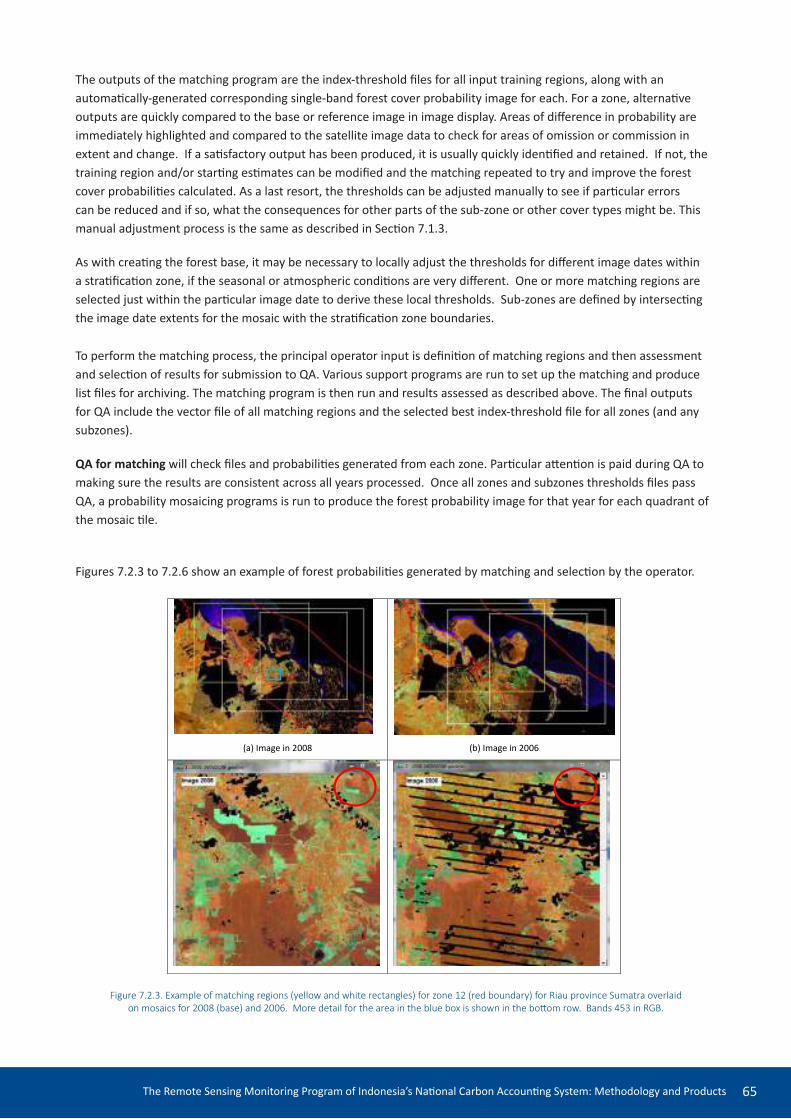
The Remote Sensing Monitoring Program of Indonesia’s Naional Carbon Accouning System: Methodology and Products 65
The outputs of the matching program are the index-threshold iles for all input training regions, along with an automaically-generated corresponding single-band forest cover probability image for each. For a zone, alternaive outputs are quickly compared to the base or reference image in image display. Areas of diference in probability are immediately highlighted and compared to the satellite image data to check for areas of omission or commission in extent and change. If a saisfactory output has been produced, it is usually quickly ideniied and retained. If not, the training region and/or staring esimates can be modiied and the matching repeated to try and improve the forest cover probabiliies calculated. As a last resort, the thresholds can be adjusted manually to see if paricular errors can be reduced and if so, what the consequences for other parts of the sub-zone or other cover types might be. This manual adjustment process is the same as described in Secion 7.1.3.
As with creaing the forest base, it may be necessary to locally adjust the thresholds for diferent image dates within a straiicaion zone, if the seasonal or atmospheric condiions are very diferent. One or more matching regions are selected just within the paricular image date to derive these local thresholds. Sub-zones are deined by intersecing the image date extents for the mosaic with the straiicaion zone boundaries.
To perform the matching process, the principal operator input is deiniion of matching regions and then assessment and selecion of results for submission to QA. Various support programs are run to set up the matching and produce list iles for archiving. The matching program is then run and results assessed as described above. The inal outputs for QA include the vector ile of all matching regions and the selected best index-threshold ile for all zones (and any subzones).
QA for matching will check iles and probabiliies generated from each zone. Paricular atenion is paid during QA to making sure the results are consistent across all years processed. Once all zones and subzones thresholds iles pass QA, a probability mosaicing programs is run to produce the forest probability image for that year for each quadrant of the mosaic ile.
Figures 7.2.3 to 7.2.6 show an example of forest probabiliies generated by matching and selecion by the operator.
(a) Image in 2008
(b) Image in 2006
Figure 7.2.3. Example of matching regions (yellow and white rectangles) for zone 12 (red boundary) for Riau province Sumatra overlaid on mosaics for 2008 (base) and 2006. More detail for the area in the blue box is shown in the botom row. Bands 453 in RGB.

The Remote Sensing Monitoring Program of Indonesia’s Naional Carbon Accouning System: Methodology and Products66
Figure 7.2.4. Example of index displays for the 2008 forest base and two outputs for 2006 from the matching process. The display shown combines in red and green the results from two indices (see Figure 7.1.5). Yellow areas indicate high forest probabiliies from both indices; black zero probability;
areas of red and green are excluded by one index and would get zero probability of forest cover. The area in the red circle in the lower map (version123) has under-classiied forest in this area compared with the base and the imagery. The top map (version121) is a beter result.
Index display from 2008 (forest base) in red and
green.
Index display from 2006 in red and green from
matching region 121.
Index display from 2006 in red and green from
matching region 123.
Based on comparison illustrated above, the results from the version 121 matching region were selected in this case. The matching program saves the indices and thresholds that correspond to each result in a text ile like that shown in Figure 7.2.5. Figure 7.2.6 shows the corresponding probability images calculated from the index displays in Figure 7.2.4 for the 2008 base and the ‘best’ 2006 result.
Figure 7.2.5. Example of an index-threshold text ile output from matching

The Remote Sensing Monitoring Program of Indonesia’s Naional Carbon Accouning System: Methodology and Products 67
Figure 7.2.7. Example. Output forest probability map for 2006 produced by matching for the area above, compared to the 2008 base
probabiliies. Red indicates high probabiliies (near 100%) while blue indicates probability zero. Missing data is shown in black.

The Remote Sensing Monitoring Program of Indonesia’s Naional Carbon Accouning System: Methodology and Products68
7.3 Muli temporal classiicaion
The individual year classiicaions of forest probabiliies are combined and reined in this stage using a mathemaical approach which combines the enire ime series of probabiliies, along with probabilisic weights relaing to accuracy, temporal change and each pixel’s neighbouring probabiliies. The output is a second set of probability images, the inal forest probabiliies, which can be thresholded and diferenced to provide extent and change maps. Models which describe probabilisic relaionships between data of this kind are known as Bayesian networks. Condiional probability networks (CPNs) are used to perform the muli-temporal processing. The CPN provides a computaional framework to combine uncertain data (relaive likelihoods derived from satellite image data from individual years). CPNs allow for the assessment and propagaion of uncertainty from muliple sources of data of varying quality or accuracy (Cacceta, 1997). The scheme for combining data was based upon techniques presented by Lauritzen and Spiegelhalter (1988) and Lauritzen (1992).
The moivaion for this processing step in a monitoring context can be summarised as follows. Each classiicaion map will contain some errors. For detecing changes between two or more maps, any errors in each map will result in erroneous changes when diferencing of hard classiicaion labels is used. Other informaion may be used to modify the probabiliies. Knowledge of temporal growth paterns in forest and non-forest land cover types provides the opportunity to improve the results of the ‘single-date’ classiicaions using a muli-temporal processing scheme. The CPN processing aims to
• improve consistency of the forest mapping from year to year so that there is less error in the land cover change products due to errors in the individual years;
• infer the most likely land cover type or land cover change year in areas of missing data due to cloud cover (missing data will be illed with a best esimate using the ime series); and
• resolve the uncertainty in the land cover at some dates by considering the informaion from the full ime series.
A key concept in using a muli-temporal processing scheme is that trees take ime to grow. A forest cannot grow and be harvested in only one year, or even two or three years. If the spectral signal is similar to forest in one year, but not the year before nor the year ater, it is unlikely to be forest. If a region is truly forest it will be forest for many years. It may stay forest (always high forest probability) or be cleared for another land use (a sequence of high forest probabiliies followed by a sudden change to a sequence of low or zero forest probabiliies). A new forest plantaion or a region of forest recovering from a severe ire will have a period of low or zero forest probabiliies followed by a year or two of increasing forest probabiliies followed by several years of high forest probability. Each of these circumstances has a clear temporal signature, as illustrated in Figure 7.3.1.
A signature that varies very rapidly between forest and non-forest cover or shows forest cover only for a single year is a very unlikely long-term trend for genuine forest cover. Temporal rules are used to weight against such areas being labelled as forest cover in any year. This strategy signiicantly reduces the amount of false change detected when comparing any two years. Similarly the temporal rules use the whole temporal sequence of probabiliies to infer the cover type of areas with ‘uncertain’ probabiliies in one or more years.

The Remote Sensing Monitoring Program of Indonesia’s Naional Carbon Accouning System: Methodology and Products 69
Figure 7.3.1. Schemaic diagram of temporal paterns of probabiliies over ime for forest and non-forest cover, and for clearing and regrowth of forest. The graphic botom right shows where this temporal patern informaion is used in the muli-temporal classiicaion model (see Figure 7.3.2).
The muli-temporal processing also uses the probabiliies for the whole ime series to infer the most likely land cover or land cover change date for years when there is no data such as in cloud gaps.
The CPN model used in the LCCA can be represented by a graph (Figure 7.3.2), where the nodes of the graph represent variables, and the edges (arrows in Figure 7.3.2) of the graph represent (condiional) independence assumpions between the variables. Note that in this example, as we do in pracice, the structure of the network is assumed. Figure 7.3.2 is further discussed below.
Neighbourhood rules
Figure 7.3.2. A pictorial representaion of a condiional probability network as a graph as applied to the forest extent and change mapping analyses. The annual sequence is represented in columns from let to right.
The botom row of Figure 7.3.2 represents the true maps of forest cover at each year; these are the desired outputs but cannot be observed directly. Values for the true maps can be inferred from the other variables. The top row is the satellite imagery. From the satellite imagery we obtain the middle row - the forest probabiliies produced from the individual year mosaics (esimates of the true forest cover maps) – through the forest base and between year matching processing.

The Remote Sensing Monitoring Program of Indonesia’s Naional Carbon Accouning System: Methodology and Products70
Figure 7.3.3. An image pair from the wet (let) and dry (right) seasons. Landsat TM bands 5,4 and 3 are shown in RGB. The graphic at the far right shows where the single-date classiicaion accuracy is used in the muli-temporal classiicaion model (Figure 7.3.2).
The graph edges or ‘arrows’ represent relaionships between the variables. Observing a paricular value for a variable provides some informaion about all the other variables to which it is connected. For example, in Figure 7.3.2, a verical orange arrow (‘edge’) connecing a single-year classiicaion with the true map of the same year represents the esimated accuracies for cover types in that ‘single-date’ classiicaion (see below). The horizontal blue arrows represent knowledge about the temporal progressions in land cover, as per Figure 7.3.1. In the case of forest cover mapping, the strength of the relaionships depends on the ime interval between the image dates. For example, less change would be expected between images a few months apart than between images several years apart.
The rules, or the relaionships between the variables, are expressed in terms of condiional probability tables. These tables (or parameters) need to be speciied. There are three types of rules, or tables, in the CPN model being used. Error rates tables link the esimated forest cover to the true forest cover at each date (verical arrows in Figure 7.3.2). Temporal rules link the true forest cover maps through ime (horizontal arrows in Figure 7.3.2). Neighbourhood rules link a pixel to its neighbouring pixels (curved arrows in Figure 7.3.2).
The temporal rules describe the relaionship between the successive true forest cover maps; and represent probabiliies that (e.g.) a forest pixel may be converted to non-forest within one year. In the current LCCA processing, these values are ixed. The probability of land cover change and the probability of land cover not changing are 0.06 and 0.94 respecively for both forest and non-forest. These parameters have been set by experimentaion to minimise the mapping of false change without omiing too much true change.
The error rates tables describe the accuracy of the forest cover maps derived from the indices and thresholds. Formally they are the probability of labelling a pixel as forest given that the true ground cover is forest and the probability of labelling a pixel as non-forest given that the true ground cover is non-forest. Both of these probabiliies have been set to 0.88 for Indonesia. Due to the way the thresholds are set to avoid omission and commission errors, this constant high value is appropriate. However this value may be modiied as discussed below.
If an image from a non-opimal ime of year is used, as illustrated in Figure 7.3.3, then the discriminaion between forest and non-forest cover may be afected. The forest appears in shades of darker green in both the images and occurs mostly in the top right of the area displayed. The image to the let is from the wet season. There is a mixture of shades of green in the forest as well as a range of shades of green throughout the adjoining agricultural lands. The image to the right is from the dry season. There are fewer shades of green in the forest and much less green in the agricultural lands. There is much greater separaion between the forest signal and the non-forest signal in the dry season image and there will be much less uncertainty and error in the classiicaion. To represent this in the muli-
The Remote Sensing Monitoring Program of Indonesia’s Naional Carbon Accouning System: Methodology and Products 71
temporal classiicaion model the error rates for the wet season image can be reduced to 0.83 or 0.75 for one or both cover types, if required. This modiicaion is only applied for years where the analyses showed reduced discriminaion between the forest and non-forest sites for most straiicaion zones. A value of 0.83 is tested irst, then 0.75 or 0.65.
Spaial probability rules (neighbourhood rules) are also implemented within the CPN. Small areas of one or two pixels classiied diferently from the majority of neighbours (e.g. as non-forest surrounded by forest) are likely to be mixed pixels or incorrect and to result in false changes over ime. Neighbourhood rules (weights based on neighbouring pixels, Kiiveri and Cacceta, 1998) modify the output probabiliies of such pixels. The weighings used are the same as implemented in the Australian forest monitoring system.
Figure 7.3.4 shows the efect of the CPN on the single-date probabiliies, and on illing cloud gaps. Data from the ive years from 2001 to 2005 are displayed. The image data shows an area in Central Kalimantan which contains wetland forest. The south-east (botom right) has been cleared for agriculture in the 1990s. Small areas are sill being cleared in the remaining natural forest. The second row in the igure shows the single-date forest probabiliies for this region for each year. Red is certain forest and dark blue is certain non-forest. The other colours show uncertain regions. Yellows and oranges indicate high probability of forest cover, light blues low probability of forest cover and green is about 50%. Black shows areas with no data – cloud gaps. The third row in the igure shows the reined probabiliies from the CPN processing, using the same colour display as the single-date probabiliies. The uncertain areas have been resolved (only red and dark blue colours are seen) and the most likely probabiliies now ill the cloud gaps.
The fourth row in the igure shows the forest extent and change products created from the CPN-reined probabiliies.

The Remote Sensing Monitoring Program of Indonesia’s Naional Carbon Accouning System: Methodology and Products72
Figure 7.3.5. A display of satellite images (top row – bands 453 in RGB), single-date forest cover probabiliies (second row – red is certain forest, through orange, yellow, green and light blue to dark blue as certain non-forest; black is no data due to cloud), reined forest cover probabiliies from
the CPN (third row – same colours as second row), forest extent and change products derived from the CPN probabiliies (fourth row – green is forest in both years, red is forest loss, blue is forest gain and the light background is non-forest in both years) and forest extent and change products derived
from the single-date forest probabiliies (botom row – same colours as fourth row with grey showing areas of missing data where change could not be calculated). The region shown is from the Central Kalimantan province.

The Remote Sensing Monitoring Program of Indonesia’s Naional Carbon Accouning System: Methodology and Products 73
Probabiliies above 50% are labelled as forest and the remainder non-forest within each year; the class labels are then compared to show forest loss and gain. Dark green areas are forest in both years compared, with forest loss shown in red and forest gain shown in blue. The light background colour is non-forest in both years. Disinct areas of forest loss and gain are apparent in each annual interval, most paricularly forest loss between 2002 and 2003. For comparison, the botom row in the igure shows the forest extent and change displays calculated directly from the single-date input probabiliies using the same threshold for forest and non-forest. Areas where change could not be calculated because one or other of the years has missing data are shown in grey. More change is shown in these ‘single-date’ change comparisons and many of these areas not also ideniied as change from the CPN probabiliies licker between forest and non-forest cover in each year. The missing data and ‘licker change’ problem in comparison with the CPN outputs clearly illustrate the value of the CPN processing for monitoring.
This processing is very computaionally intensive (more than a day on a regular desktop computer) and so is performed on a high-performance blade server cluster computer system where muliple processors perform the computaions in parallel. This reduces the compute ime to less than one hour. Spaially the processing units are the quadrants for each mosaic ile to it within memory limitaions on the cluster.
CPN processing commences when the matching process is complete for all ime periods for the mosaic. In update mode, the new dates are added and the enire ime series is reprocessed. The outputs from the muli-temporal processing are the temporal set of forest probability images, one for each year, where the probabiliies of forest cover have been reined by the rules to provide temporally consistent esimates.
The products for forest extent and change maps which are derived from these outputs are described in Secion 7.4. The feedback from reviews of the 2000-2009 products is discussed in Secion 8.
The Remote Sensing Monitoring Program of Indonesia’s Naional Carbon Accouning System: Methodology and Products74
7.4 Descripion of Products
As noted above, the outputs from the muli-temporal processing are raster probability images, one for each year, where the probabiliies of forest cover have been reined by the rules to provide temporally consistent cover esimates.
The inal products required are maps (or masks) that are indicators of forest extent at each year, and forest loss (clearing) and forest gain (revegetaion) between successive years. The ime series of probabiliies are processed together to produce these products as binary raster maps; coded as (1) or (0). These can be displayed as convenional maps (below). In the conversion process, thresholds are applied to each year’s probabiliies to produce the extent map and diferencing of these results to produce the annual change products. It is noted here that the CPN processing ills almost all areas where data were missing in the mosaics, but that in this conversion, any pixels for which there was no input data in any year are recoded to 99 in the conversion. The conversion process is fully automated.
The products are produced in both the local NUTM projecion and geodeic projecion. The iles in the geodeic projecion are mosaiced into whole island regions. The resoluion of all LCCA products in NUTM is 25m, in geodeic it is 0.000025 degrees.
The key products created are:
• Forest extent maps for each year (2000, 2001, 2002, ...)
• Forest loss maps for each annual period (2000-2001, 2001-2002, ...)
• Forest gain maps for each annual period (2000-2001, 2001-2002, ...)
• Year of irst forest loss
• Year of irst forest gain
The year of forest irst forest loss and gain are stored as integers counted from the beginning of the ime series. For example, a change in the 2000-2001 interval is stored as 1 and 2001-2002 is stored as 2.
Staisical summaries at naional, regional and local scales can be calculated directly from these products in GIS systems. Staisical and map summaries may be produced by a range of users for various purposes. Staisical summaries are not standard LCCA products, but examples are provided here for illustraion.
An example of each product is presented and discussed below.
Annual Forest Extent. Figure 7.4.1 shows the 2009 forest extent product for Indonesia, and for Kalimantan as a regional example. There is a forest extent product for each year in the ime series.

The Remote Sensing Monitoring Program of Indonesia’s Naional Carbon Accouning System: Methodology and Products 75
Figure 7.4.1. Illustraion of forest extent (2009) at naional, regional and local scale. The local scale includes comparison with Landsat and high resoluion imagery.
Annual forest loss and gain. Forest loss (clearing or harvesing) and forest gain (regrowth or replaning) products are produced for each annual interval in the ime series, e.g. 2000-2001, 2001 – 2002. This can be displayed as total forest change over a number of years as in Figure 7.4.2, and Figure 7.4.3, or year by year change maps as in Figure 7.4.4.

The Remote Sensing Monitoring Program of Indonesia’s Naional Carbon Accouning System: Methodology and Products76
Figure 7.4.2. Total forest loss and gain 2000-2009 at naional scale from the LCCA. Dark green indicates areas that were always forest from 2000 to 2009, red shows forest loss between 2000 and 2009 while yellow indicates forest gain in the same period. [source: INCAS poster, Workshop on Earth
Observaion Satellite Data to Support REDD+ Implementaion in Indonesia, February 2014]
Figure 7.4.3 Forest loss and gain for 2000-2009 at regional scale. Dark green indicates areas that were always forest from 2000 to 2009, red shows forest loss between 2000 and 2009 while yellow indicates forest gain in the same period. [source: INCAS poster, Workshop on Earth Observaion
Satellite Data to Support REDD+ Implementaion in Indonesia, February 2014]

The Remote Sensing Monitoring Program of Indonesia’s Naional Carbon Accouning System: Methodology and Products 77
Figure 7.4.4 Forest loss and gain for 2002-2003 at local scale. The region shown is in the Central Kalimantan province. As in the igures above, green is forest in 2002, red is forest loss from 2002 to 2003 and yellow is forest gain from 2002 to 2003. The background colour is non-forest.
Figure 7.4.5. Year of irst forest loss and gain at regional scale coloured by year of change as indicated in the legend above.
Year of irst forest loss and gain. This product ideniies the year of irst change in forest cover within the ime series. It was developed speciically for the carbon accouning stage of the INCAS program. In the forest gain product, it provides a planing date for new plantaions or a regrowth date for disturbed forest. In the forest loss product it provides a year of disturbance. Deciding whether the date is the irst disturbance of natural forest or the harvest date of already disturbed forest or a plantaion requires some outside knowledge of the state of the forest at the beginning of the ime series.

The Remote Sensing Monitoring Program of Indonesia’s Naional Carbon Accouning System: Methodology and Products78
Staisical summaries. The area of forested land or forest extent change can be calculated from the LCCA products and presented in tabular and graph formats. Once again, these summaries can be made at naional, regional and local levels as shown in Table 7.4.1 and Figure 7.4.6. These examples are provided for illustraion purposes only and are not inal results.
Time Period Forest Loss (hectares) Forest Gain (hectares)2000-2001 46002.977 75737.9292001-2002 111206.196 104178.5232002-2003 155917.199 102938.2272003-2004 145241.838 111251.4472004-2005 119986.428 114067.9852005-2006 195822.295 60392.2662006-2007 183959.252 57955.6072007-2008 231188.88 40375.6922008-2009 238340.948 64201.398
Table 7.4.1: Sample Forest Change Summary for Sulawesi
Figure 7.4.6. Sample graph of total areas of naional forest loss and gain by year, 2000-2009.

The Remote Sensing Monitoring Program of Indonesia’s Naional Carbon Accouning System: Methodology and Products 79
8. REVIEW OF THE PRODUCTS
A key element of any mapping program is the accuracy of the maps produced. A formal accuracy assessment methodology – for both forest extent and change – is yet to be agreed. Understanding of accuracy, uncertainty and error is criical for use of maps in diferent policy contexts. Understanding of error also may feed back into a coninuous improvement process. In the LCCA, there has been formal interacion with local experts to get feedback on the 2000-2009 version of the products. We are acing on the issues ideniied in this feedback to improve the accuracy of the 2000-2012 version of the products. The review process, which combines ground knowledge and the image processing experience which generated the products, fulils two major roles within coninuous improvement. They are:
1. it may idenify errors which can be corrected by revising steps in the current process (e.g. straiicaion or thresholds for a zone), or it may idenify errors or uncertainies which suggest need for invesigaion of new methods.
2. it may idenify and locate paricular ground cover types where spectral data cannot adequately classify the desired cover types, and errors in the extent of change results. Locaion of these cover types (e.g. by drawing vectors) provides a basis to remove paricular errors of this kind, and, where required for paricular purposes, to seek other informaion to idenify and reduce such errors as far as possible.
This secion of the documentaion describes in some detail the review process to date. It provides summaries and examples of the major issues ideniied and how this informaion has been used to improve the new products.
8.1 Expert review
A product review workshop was held for each island region, namely Kalimantan, Sumatra, Papua, Sulawesi, Java, Nusa Tenggara and North and South Maluku. There were three main aims for these workshops:
(i) to get feedback on the accuracy of the forest extent and change products, idenifying issues that we could ix and issues that must be accepted as limitaions of the methodology;
(ii) for the irst prospecive users to get an understanding of the strengths and limitaions of the products; and
(iii) to start to understand what ancillary data is required to use these products for the purpose of carbon accouning.
Carbon accouning rules typically require consideraion of why or how the land cover changes – is it human-induced land use change (perhaps from natural forest to rice cropping) or land cover change caused by nature (perhaps a tsunami washes away mangrove forest). Our satellite mapping ‘sees’ what has changed and when, but has less informaion on how or why the change occurred. This ‘atribuion’ of the land cover change is considered more completely as part of the carbon accouning part of the INCAS program, but some of the ideas were introduced at these workshops to discover if there were datasets available that would aid in the atribuion.
The main outcomes from the forest review workshops are annotated forest change maps and an acion list for the processing team of issues that should be considered when the products are next updated. During the workshop, the annotaion occurs on paper maps printed from the digital products as can be seen in Figure 8.1.1. These regions are later digiised for easy overlay on the electronic products. Issues for acion are ideniied in lists like that shown in Table 8.1.1.
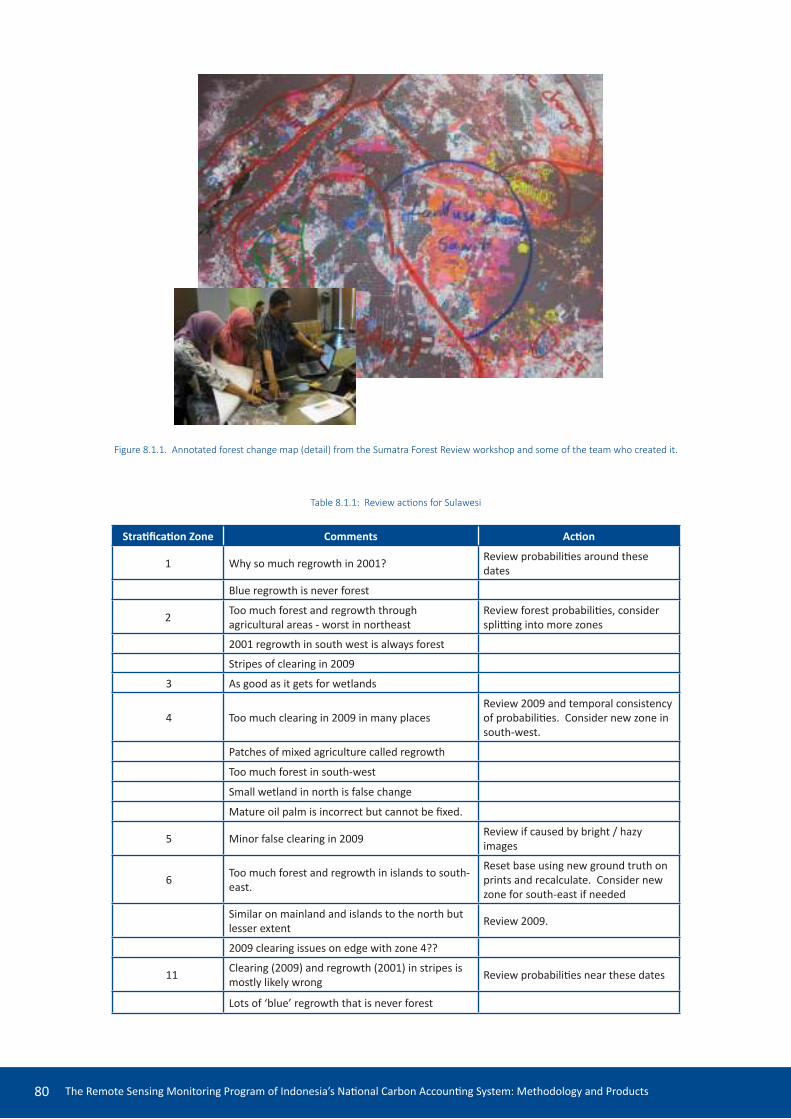
The Remote Sensing Monitoring Program of Indonesia’s Naional Carbon Accouning System: Methodology and Products80
Figure 8.1.1. Annotated forest change map (detail) from the Sumatra Forest Review workshop and some of the team who created it.
Table 8.1.1: Review acions for Sulawesi
Straiicaion Zone Comments Acion
1 Why so much regrowth in 2001? Review probabiliies around these dates
Blue regrowth is never forest
2 Too much forest and regrowth through agricultural areas - worst in northeast
Review forest probabiliies, consider spliing into more zones
2001 regrowth in south west is always forest
Stripes of clearing in 2009
3 As good as it gets for wetlands
4 Too much clearing in 2009 in many placesReview 2009 and temporal consistency of probabiliies. Consider new zone in south-west.
Patches of mixed agriculture called regrowth
Too much forest in south-west
Small wetland in north is false change
Mature oil palm is incorrect but cannot be ixed.
5 Minor false clearing in 2009 Review if caused by bright / hazy images
6Too much forest and regrowth in islands to south-east.
Reset base using new ground truth on prints and recalculate. Consider new zone for south-east if needed
Similar on mainland and islands to the north but
lesser extentReview 2009.
2009 clearing issues on edge with zone 4??
11 Clearing (2009) and regrowth (2001) in stripes is mostly likely wrong Review probabiliies near these dates
Lots of ‘blue’ regrowth that is never forest

The Remote Sensing Monitoring Program of Indonesia’s Naional Carbon Accouning System: Methodology and Products 81
Forest review workshops are a collaboraive efort between expert groups. Paricipants include:
• People from LAPAN who are part of the processing teams who make the products. They are the experts in how the products were made, and what cover types could and couldn’t be easily separated in the available image data.
• People from the MoF represening the teams who will be potenial users of the data for both carbon accouning and other purposes.
• People from naional and local agencies who know the land cover and the land use in the regions being reviewed.
Some of the people from the MoF and from the regions were part of the team providing local input to the creaion of the forest base and some were people new to the project at this review stage.
Maps of iniial forest extent and the year of irst forest loss or forest gain (see Figure 8.1.2) were printed in large format to cover the whole region being reviewed at a scale where local change events and landmarks could be recognised by the team.
The experts come together around the printed maps. The ground experts consider where the maps are right and where the maps are wrong:
• Is the forest extent broadly correct? Are there areas of forest that are omited? Are there regions mapped as forest that are not forest?
• Is the change extent and iming broadly correct? Are there areas mapped as change that were always forest or never forest? Are the areas of known change included in the maps?
• Is there ancillary data that can be accessed by the processing team to support the expert opinions? Can this data be used to help with atribuing the cause of the change?
The data analysis experts consider the areas where the maps are found to be inaccurate. Together with the ground experts, they consider if the errors can be ixed. Are they caused by limitaions in the separability of some cover types in the available satellite imagery? Is it because of how the forest (or non-forest cover) grows, e.g. deciduous forest, or how the forest is managed, e.g. teak and cinnamon? Is it because of some error or misunderstanding in the data processing and the methodology can be improved? The acion lists (Table 8.1.1) are the summaries of these discussions.
Figure 8.1.2: Year of irst forest loss and gain at regional scale coloured by year of change as indicated in the legend above.

The Remote Sensing Monitoring Program of Indonesia’s Naional Carbon Accouning System: Methodology and Products82
The conversaions are recorded by annotaing the printed maps (Figure 8.1.3). This includes an outline of the region being discussed and a very short descripion of the issue (a true cover type, date of change or conirmaion of the change and the new cover type). Any ancillary datasets relaing to the issue are collected. A digiising person is assigned to each working group who will later convert the drawings to vectors. Oten the printed maps are scanned as an addiional record of the process.
Although they do not provide a formal accuracy assessment, these forest review workshops provide invaluable feedback on errors in the products, both in forest extent, land use change and the iming of the change.
Figure 8.1.3. Annotaion of forest extent and change maps during the forest review workshops.

The Remote Sensing Monitoring Program of Indonesia’s Naional Carbon Accouning System: Methodology and Products 83
8.2. Issues and acions ideniied
The main issues recognised during the forest review workshops are discussed below. They relate to problemaic cover types (palms, wetlands, shrubs, deciduous forest, some forest management pracices) where operaional soluions are suggested, and to ‘processing learning errors’ which highlighted where current operator processes could be improved.
8.2.1 Cover type - palms
Young palms are spectrally separable from forest cover types in the Landsat image data, but the spectral signal of mature palms typically becomes more like the spectral signal of some of the true forest. This is essenially a limitaion of the current products, but various strategies are considered to restrict the consequences of the error.
In Kalimantan and Sumatra the most common types of palms are oil palms (sawit). The clearing of forest prior to the planing of new oil palm is accurately detected and the land cover of the new oil palm plantaion is mapped as non-forest for the irst three to ive years. Ater that, the plantaion signal becomes more like forest and plantaions appear as forest regrowth in the LCCA products. The simplest strategy here is to obtain or produce an oil palm extent map from another source. The oil palm map can be used to mask the regrowth in the LCCA product and the LCCA product can return a date of planing for new oil palm plantaions. An alternaive is to invesigate palm mapping using other data sources (e.g. radar data) and integrate such data products into the LCCA processing stream.
Coconut palms (kelapa) are common in Sumatra and other parts of Indonesia. There are far fewer new plantaions than for oil palm so most of the exising palm fall into the ‘mature’ category. They are also frequently grown together with tree crops in ‘mixed’ agricultural areas. Straiicaion zones are used to separate the major coconut palm cropping areas from the surrounding forest. Large commercial planings predominantly occur in low lying coastal areas with boundaries that can be relaively easily deined. These regions may include coastal mangroves; however mangrove forests and coconut palms are spectrally separable. In the smaller, ‘mixed planings’ regions the forest extent is either under- or over-esimated depending on whether there are more tree crops / natural forest or more palms.
Sagu and nipah palms are found naturally mixed into the forest in Papua. Spectrally they are very similar to forest, paricularly when it is wet, and their co-occurrence with trees tests ‘canopy density’ limits in the deiniion of forest. They are part of the long-term natural cover and so temporal paterns cannot be used to separate the palms from the forest. Typically the regions are labelled forest which avoids inconsistencies causing false change.
8.2.2 Cover type -wetlands
In the wet season when wetlands are full of water, the spectral signal is very diferent to forest. In the dry, when the surface is bare of water, the spectral signal is also very diferent to forest. In between these two imes, the cover is oten green vegetaion (grasses or reeds) growing in shallow surface water. This paricular mixture of green vegetaion and dark water signals appears very similar to the spectral signature of wetland forest types. What makes the forest diferent to wetlands is that the spectral signal from the wetland forest is relaively constant from year to year and from season to season but the signal of the other wetland vegetaion varies from season to season and year to year. However, if the best available images are during the transiion from wet to dry for several years in sequence, a sequence of ‘forest-like’ signals build and wetlands can be misclassiied as forest. As this signal doesn’t persist for as long as true forest, the products tend to show muliple regrowth and clearing events over many wetland areas.
Similar spectral confusion can arise in rice growing areas. When the paddy is looded or completely dry, the spectral signal is very diferent to forest. When there is a mixture of water and green shoots, the spectral signal becomes more like forest. When the water recedes and there is just green crop, the signal is diferent to forest again. Unlike wetlands,

The Remote Sensing Monitoring Program of Indonesia’s Naional Carbon Accouning System: Methodology and Products84
major rice growing areas are geographically well separated from forest and straiicaion zone boundaries can usually be used to provide separaion from forested areas. Wetlands tend to be much more ‘mixed’ into natural forest environments and straiicaion is not an eicient opion. However, knowledge of these wetland locaions as a spaial database can be built up using imagery and other data. Sourcing or developing a separate wetlands map (perhaps considering only wet season imagery and terrain) and using it to mask the false change is currently the recommended strategy.
8.2.3 Cover type - shrublands
The main diference between trees and shrubs is height; hence shrublands are excluded from forests by the height component of the forest deiniion. The Landsat imagery provides no informaion on vegetaion height. Ground truth informaion (the shadows in high resoluion imagery give an indicaion of feature height) and local knowledge are used to idenify the major regions of shrubs with litle (below 30%) or no tree cover. Straiicaion zone boundaries are again used to separate such regions from forest (more than 30% trees even if some shrubs are also present). Where there is a natural separaion of trees and shrubs or historical land clearing has created an ariicial separaion, this strategy is efecive. Where there is a coninuum of cover from trees to shrubs, a choice is made to map the area as either forest or not forest depending on which minimises the error in the overall forest extent.
8.2.4 Cover type - deciduous forest
Deciduous forests lose their leaves during some part of the year. In Indonesia such species usually lose their leaves during the dry season. This occurs with teak (jai) forests, predominantly in the eastern half of Java and other species in eastern Java, Bali and parts of Nusa Tenggara and Maluku. If imagery is captured during the dry season, there is litle or no canopy and the majority of the signal is from the ground below the tree. The signal is very unlike forest. In the wet season, there is full canopy cover and a strong forest signal. As several image dates are required to build cloud-free composite images within each year, there is limited ability to select seasonally-consistent image dates. Local knowledge has been used to create straiicaions zones that separate deciduous forest from other forest types. Within these zones we try to use the understorey signal to map deciduous forest as forest even in the dry season. Even with these strategies, the amount of false change mapped is higher in deciduous forests than in non-deciduous forests.
8.2.5 Cover type and management - forest management pracices
There are two main examples of forest management pracices afecing the accuracy of the forest extent and change mapping. The irst example is teak (jai) forest management. The quality of the wood depends on the amount of sunlight it receives. Trees are planted further apart to minimise the shadow of one tree falling on another tree, decreasing canopy density in a plantaion. The ground beneath and between the trees is used for other agricultural crops, further confusing the signal received. Combined with the deciduous nature of the teak forests in some regions, these forests are diicult to map consistently. There are errors in both forest extent and change in such forests. Straiicaion zone boundaries are used to separate these forests from other cover, but the recommended soluion is to seek or develop an independent teak forest extent map. As a very high value imber resource, informaion on its extent is likely to be available. Depending on quality and currency, such a map may be used to mask false change rather than adjusing the forest extent.
The other example of forest management pracices causing more error is in cinnamon forests. Coppicing - cuing young tree stems down to near ground level to encourage many new shoots - is used to maximise the area of new young bark that contains the cinnamon spice. The cuing in cinnamon forests can occur every two to three years. Images acquired ater cuing show bare stumps and litle or no canopy. Large plantaion areas have litle or no

The Remote Sensing Monitoring Program of Indonesia’s Naional Carbon Accouning System: Methodology and Products 85
temporal consistency in their forest / not forest signal. Again, straiicaion zones are used to separate the major plantaions in Sumatra and atempts made to treat the ‘cut’ signal as forest. Natural cinnamon has a less regular cuing patern and there is usually enough canopy and surrounding trees to allow more reliable mapping.
8.2.6 Learning errors – processing and skills improvement
It should be noted that the irst naional products (2000-2009) were created by teams trying to both master new processing methodologies and adapt those methodologies from an Australian / internaional applicaion to Indonesian speciic condiions while being required to meet ight processing deadlines.
Processing errors were made iniially that the now-experienced teams would detect and correct before product creaion, but the learning experience requires inding the consequences of those mistakes to develop the judgement and understanding of how to look for the errors and either prevent them or discover and ix them in a imely fashion.
Many of the ideniied errors all fall into the ‘easily ixable’ category. Strategies, in the form of processing sotware, operator review and QA, have been developed to prevent many of these errors. In the update processing (for years 2010-2012) these strategies have already been implemented and the errors themselves are being corrected at the same ime as the new data is being processed. Improvements in eiciency and product consistency have resulted.

The Remote Sensing Monitoring Program of Indonesia’s Naional Carbon Accouning System: Methodology and Products86
8.3 Product improvement
There are two aspects to a ‘coninuous improvement’ program. One aspect is to take feedback from product review and any formal accuracy assessments and review the data processing to correct as many of the errors as possible. How this is being done in the LCCA program is discussed here. The second aspect of ‘coninuous improvement’ is to review the methodology and the eiciency of its implementaion to make the processing as eicient and accurate as possible. The plans for this are discussed as part of Secion 2 ‘Status and Future Direcions’.
The relevant outcomes from the Forest Review workshops are a list of problems found in the products for a paricular region and the spaial locaion of the errors (Figure 8.1.1 and Table 8.1.1 in the preceding secion). From these lists we can prioriise acions to address the problems. The factors considered in deciding what acion to take and when include:
• the spaial extent of the problem;
• the availability of a soluion;
• the ime required to implement the soluion; and
• the sensiivity of the subsequent purpose (or purposes) to the problem.
Fixing a problem that covers a large area spaially will provide a greater improvement to the products overall than working irst on problems that are very localised. However, the size of the error is not the only consideraion. Oten local problems have quite simple soluions that are quick to implement. For example, several areas of mangrove forest along the south-east coast of Sumatra were mapped as non-forest in the 2000-2009 (version 1) products. The extent of the area omited from the forest extent is quite small compared to the area of false change in cinnamon forests in south western parts of Sumatra (Figure 8.3.1).
Figure 8.3.2 shows the original straiicaion zone map for Sumatra. There are straiicaion zones for mangroves in the north-east (zone 28) and mangroves versus coconut palms along the eastern part of the north coast (zone 2), but no such straiicaion zone in the south-east. The soluion to the omited mangrove forests is simply to create a new mangroves zone (now called zone 29) and copy the indices from the exising mangrove zone. Experience in other parts of Indonesia shows that mangrove forest can be mapped very accurately when suitable straiicaion zones are used.
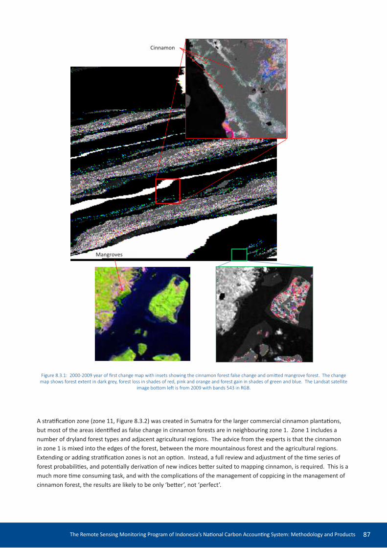
The Remote Sensing Monitoring Program of Indonesia’s Naional Carbon Accouning System: Methodology and Products 87
Cinnamon
Mangroves
Figure 8.3.1: 2000-2009 year of irst change map with insets showing the cinnamon forest false change and omited mangrove forest. The change map shows forest extent in dark grey, forest loss in shades of red, pink and orange and forest gain in shades of green and blue. The Landsat satellite
image botom let is from 2009 with bands 543 in RGB.
A straiicaion zone (zone 11, Figure 8.3.2) was created in Sumatra for the larger commercial cinnamon plantaions, but most of the areas ideniied as false change in cinnamon forests are in neighbouring zone 1. Zone 1 includes a number of dryland forest types and adjacent agricultural regions. The advice from the experts is that the cinnamon in zone 1 is mixed into the edges of the forest, between the more mountainous forest and the agricultural regions. Extending or adding straiicaion zones is not an opion. Instead, a full review and adjustment of the ime series of forest probabiliies, and potenially derivaion of new indices beter suited to mapping cinnamon, is required. This is a much more ime consuming task, and with the complicaions of the management of coppicing in the management of cinnamon forest, the results are likely to be only ‘beter’, not ‘perfect’.

The Remote Sensing Monitoring Program of Indonesia’s Naional Carbon Accouning System: Methodology and Products88
Figure 8.3.3. Original and improved year of irst change maps for the inset areas in Figure 8.3.1. The change map shows forest extent in dark green (top) or dark grey (botom), forest loss in shades of red, pink and orange and forest gain in shades of green and blue. In version 2, the mangrove
forests are no longer omited and the cinnamon forests appear as stable forest instead of forest regrowth.
Figure 8.3.2. Straiicaion zone map from creaing the Sumatra 2000-2009 (version 1) products.
Both of these problems were addressed and improved in creaing the 2000-2012 (version 2) products for Sumatra. Figure 8.3.3 shows the new products.
Version 1 (2000-2009)
Version 2 (2000-2012)
Version 1 (2000-2009)
Version 2 (2000-2012)

The Remote Sensing Monitoring Program of Indonesia’s Naional Carbon Accouning System: Methodology and Products 89
The most eicient ime to make correcions to the processing and products is when an addiional year is being added to the ime series. Correcions to the version 1 products were made for each island group as part of the update when data for 2010, 2011 and 2012 were added to the ime series. The expert reviews can be revisited, comparing the original and new products. The lists of issues with the products are updated to recognise the correcions, and perhaps new issues that are now apparent once other issues are resolved are added. Policy consideraions of diferent users may provide clear prioriies for eforts to implement correcions, either within the image processing stream or by using other data. For carbon accouning, a means to idenify oil palm from forest (as discussed above) may be a high priority, while for coastal habitat management, accurate maps of mangroves may be a priority.
This intenion is an ongoing program of reviewing the products, both informally and formally when possible, and acing on the feedback from those reviews to improve the products over ime.

The Remote Sensing Monitoring Program of Indonesia’s Naional Carbon Accouning System: Methodology and Products90

The Remote Sensing Monitoring Program of Indonesia’s Naional Carbon Accouning System: Methodology and Products 91
9. REFERENCES
Cacceta, P. A., Furby, S. L., O’Connell, J., Wallace, J. F. and Wu, X. (2007). Coninental Monitoring: 34 Years of Land Cover Change Using Landsat Imagery. Paper presented at the 32nd Internaional Symposium on Remote Sensing of Environment, June 25-29, 2007, San Jose. Costa Rica.
Cacceta P.A. 1997, Remote sensing, geographic informaion systems (GIS) and Bayesian knowledge-based methods for monitoring land condiion. Ph.D. thesis. School of Compuing, Curin University of Technology, Perth, WA, Australia.
Cacceta, P.A. Furby, S.L, Wallace, J.F., Wu, X, Richards, G., and Waterworth, R. 2013. Long-Term Monitoring of Australian Land Cover Change Using Landsat Data: Development, Implementaion, and Operaion. In: Achard F. & Hansen M.C (eds). Global Forest Monitoring from earth Observaion, chapter 13. Taylor & Francis. New York.
Campbell, N.A., and Atchley W.R. 1981. The geometry of canonical variate analysis. Syst. Zool. 30(3): 268-280.
Danaher, T., Wu, X. and Campbell, N. A. (2001). Bidirecional Relectance Distribuion Funcion Approaches to Radiometric Calibraion of Landsat TM Imagery. In: Proceedings of the Internaional Geoscience and Remote Sensing Society Symposium, Sydney, Australia, July 2001.
Furby, S.L. 2002. Land Cover Change: Speciicaion for remote sensing analysis. Naional Carbon Accouning System Technical Report 9. Australian Greenhouse Oice, Canberra.
Furby, S.L, Cacceta, P.A. and Wallace, J.F. 2010. Salinity Monitoring in Western Australia using Remotely Sensed and Other Spaial Data. J Environ. Quality, 39, pp16-25.
Gutman, G., Byrnes, R., Masek, J., Covington, S., Jusice, C., Franks, S., and Headley, R.. 2008. Towards Monitoring Land-cover and Land-use Changes at a Global Scale: The Global Land Survey 2005. Photogrammetric Engineering & Remote Sensing, January 2008.
Hansen M.C, Roy D.P., Lindquist E., Adusei B., Jusice C.O., and Altstat, A. 2008. A Method For Integraing MODIS and Landsat Data for Systemaic Monitoring of Forest Cover Change in The Congo Basin. Remote Sensing of Environment, 112, 2495-2513.
Irish, R.R., Barker, J.L., Goward S.N.,and Arvidson, T. 2006. Characterizaion of the Landsat -7 ETM+ Automatwd Cloud-Cover Assessment (ACCA) Algorithm. Photogrammetric Engineering and Remote Sensing, 72, no 10, pp1179-1188.
Kiiveri, H.T., and Cacceta, P.A. 1998. Image fusion with condiional probability networks for monitoring salinisaion of farmland. Digial Signal Processing. 8(4):225–230.
Kiiveri, H.T., Cacceta, P.A., and Evans F.H. 2001. Use of condiional probability networks for environmental monitoring. Internaional Journal of Remote Sensing. 22(7):1173–1190.
Kiiveri, H.T., Cacceta, P.A., N.A. Campbell, Evans F.H., Furby S.L., and Wallace, J.F. 2003. Environmental monitoring using a ime series of satellite images and other spaial data sets. p. 49–62. In: D.D. Denison et al (eds) Nonlinear esimaion and classiicaion by lecture notes in staisics. Springer Verlag, New York.
Lauritzen, S.L. 1992. Propagaion of probabiliies, means and variances in mixed graphical associaion models. Journal of the American Staisical Associaion. 87(420):1098-1108.
Lauritzen, S.L., and D.J. Spiegelhalter. 1988. Local computaions with probabiliies on graphical structures and their applicaion to expert systems. Journal of the Royal Staisical Society. Series B 50(2):157-224.

The INCAS-LCCA Remote Sensing Monitoring Program: Methodology and Products92
Marinuzzi S, Gould, W.A., and Ramos González O.M. 2007. Creaing Cloud-Free Landsat ETM+ Data Sets in Tropical Landscapes: Cloud and Cloud-Shadow Removal, USFS IITF-GTR32.
O’Connell, J. and Cacceta, P. A. (2009), Tesing of Alternate Classiicaion Procedures within an Operaional, Satellite based, Forest Monitoring System. In: ‘Innovaions in Remote Sensing and Photogrammetry’, Lecture Notes in Geoinformaion and Cartography, 121-132, Springer Verlag Berlin Heidelberg, ISBN 978-3-540-88265-7.
Teillet, P.M., Guindon, B., Goodenough, D.G., 1982, On the Slope-Aspect Correcion of Mulispectral Scanner Data, Canadian Journal of Remote Sensing, 8(2), 84-106.
Townshend, J. R. G., C. O. Jusice, W. Li, C. Gurney, and J. McManus, 1992. The impact of misregistraion on the detecion of changes in landcover. IEEE Transacion on Geoscience and Remote Sensing, 30:1054–1060.
Tucker, Compton, J., Grant, Denelle M., and Dykstra, Jon D. (2004). NASA’s Global Orthoreciied Landsat Data Set, Photogrammetric engineering and Remote Sensing, Vol 70, No. 3, March 2004, pp.313-322.
USGS 2009, Global Land Survey, 2000, Landsat ETM+, USGS, Sioux Falls, South Dakota.
Vermote, E., D. Tanré, J. L. Deuzé, M. Herman, and J.J. Morcrete, Second Simulaion of the Satellite Signal in the Solar Spectrum (6S), 6S User Guide Version 0, April 1994.
Wang, B, Ono, A, Muramatsu, K, and Fujiwara, N. Automated Detecion and Removal of Clouds and Their Shadow from Landsat TM Images. IEICE Trans. Inf. & Systems, 28, E82-D, pp453-460.
Wu, X., Furby, S. and Wallace, J.F. 2004. An approach for terrain illuminaion correcion. In: Proceedings of the 12th
Australasian Photogrammetry and Remote Sensing Conference. Fremantle Western Australia.
Wu, X. (2008). A Simpliied Ortho-Reciicaion Approach for Satellite Imagery. In: Proceedings of the XXI Congress of the Internaional Society for Photogrammetry and Remote Sensing Vol.IIIa, pp.1-6, 3-11 July, 2008.Beijing, China.


