the reliability of voluntary disclosures: evidence from...

The Reliability of Voluntary Disclosures:

Evidence from Hedge Funds�

Andrew J. Patton, Tarun Ramadorai, and Michael Streat�eldy

First Draft: 27 September 2011.

Current Draft: 4 November 2011

Abstract

We analyze the reliability of voluntary disclosures of �nancial information, focusing on widely-

employed publicly available hedge fund databases. Tracking changes to statements of historical

performance recorded at di¤erent points in time between 2007 and 2011, we �nd that histor-

ical returns are routinely revised. These revisions are not merely random or corrections of

earlier mistakes; they are partly forecastable by fund characteristics. Funds that revise their

performance histories signi�cantly and predictably underperform those that have never revised,

suggesting that unreliable disclosures constitute a valuable source of information for current

and potential investors. These results speak to current debates about mandatory disclosures by

�nancial institutions to market regulators.

�We thank John Campbell, Evan Dudley, Terry Lyons, Ludovic Phalippou, Neil Shephard and seminar participantsat UNC-Chapel Hill and Vanderbilt University for comments and suggestions. Sushant Vale provided excellentresearch assistance.

yPatton is at Department of Economics, Duke University, and Oxford-Man Institute of Quantitative Finance.Email: [email protected]. Ramadorai is at Saïd Business School, Oxford-Man Institute, and CEPR.Email: [email protected]. Streat�eld is at Saïd Business School and Oxford-Man Institute. Email:michael.streat�[email protected]

I. Introduction

In January 2011 the Securities and Exchange Commission proposed a rule requiring U.S.-based

hedge funds to provide regular reports on their performance, trading positions, and counterparties

to a new �nancial stability panel established under the Dodd-Frank Act. A modi�ed version of this

proposal was voted for adoption in October 2011, and will be phased in starting late 2012. The

proposal requires detailed quarterly reports (using new Form PF) for 200 or so large hedge funds

� those managing over U.S.$1.5 billion �which collectively account for over 80% of total hedge

fund assets under management; and for smaller hedge funds, these reports will be less detailed, and

required only annually. The proposal states clearly that the reports would only be available to the

regulator, with no provisions in the proposal regarding reporting to funds�investors. Nevertheless,

hedge funds argued against the proposal, citing concerns that the government regulator responsible

for collecting the reports could not guarantee that their contents would not eventually be made

public.1

The economic theory literature almost uniformly predicts that providing more information

to consumers is welfare enhancing (an early example is Stigler (1961), also see Jin and Leslie

(2003, 2009) and references therein). Hedge funds, however, are notoriously protective of their

proprietary trading models and positions, and generally disclose only limited information, even to

their own investors. One important piece of information that many hedge funds do o¤er to a wider

audience is their monthly investment performance. This information (as well as information on

fund characteristics and assets under management),2 is self-reported by thousands of individual

hedge funds to one or more publicly available databases. These databases are widely used by

researchers, current and prospective investors, and the media. As SEC rules preclude advertising

by hedge funds, disclosing past performance and fund size to these publicly available databases is

thought to be one of the few channels that hedge funds can use to market themselves to potential

new investors (see Jorion and Schwarz (2010) for example).

In this paper, we examine the reliability of these voluntary disclosures by hedge funds, by track-

ing changes to statements of performance in the publicly available hedge fund databases recorded

at di¤erent points in time between 2007 and 2011. In each �vintage� of these databases,3 hedge

1See SEC press releases 2011-23 and 2011-226, available at www.sec.gov/news/press.shtml. For response from thehedge fund industry, see �Hedge Funds Gird to Fight Proposals on Disclosure�, Wall Street Journal, February 3 2011.

2Note that the information provided does not include the holdings or trading strategies of the fund.3This has links with the �real time data�literature in macroeconomics, see Croushore (2011) for a recent survey.

1

funds provide information on their performance from the time they began reporting to the database

until the most recent period. We �nd evidence that in successive vintages of these databases, older

performance records (pertaining to periods as far back as �fteen years) of hedge funds are routinely

revised. This behavior is widespread: nearly 40% of the 18,382 hedge funds in our sample have

revised their previous returns by at least 0.01% at least once, and over 20% of funds have revised a

previous monthly return by at least 0.5%. While positive revisions are also commonplace, negative

revisions are more likely and larger when they occur, i.e., on average, initially provided returns

present a more rosy picture of hedge fund performance than �nally revised performance. Moreover,

these revisions are not random, indeed, we employ information on the characteristics and past

performance of hedge funds to predict them. For example, funds in the Emerging Markets style

are signi�cantly more likely to have revised their histories of returns than Fixed Income funds, and

larger funds, more volatile funds, and less liquid funds are all more likely to revise.

To provide an example of the sort of episode to which we refer, consider the (anonymized but

true) case of Hedge Fund X, which was incorporated in the early 1990s. Four months later the fund

began reporting to a database, and a year after inception it reported assets under management

(AUM) in the top quintile of all funds. In the mid 2000s, the fund experienced a troubled quarter

and saw its AUM halve in value. It then ceased reporting AUM �gures. The fund�s performance

recovered, and during the last quarter of 2008 it reported a particularly good double digit return,

putting it in the top decile of funds. However a few months later this high return was revised

downward signi�cantly, into a large negative return. A similar pattern emerged later that year,

when a previously reported high month return was substantially adjusted downward in a later

vintage, along with two other past returns altered. A further sequence of poor returns was then

revealed, and the fund was �nally reported as closed in 2009.

The example provided above suggests that these revisions should be interpreted as negative

signals by investors, that is, that they are manifestations of the asymmetric information problem

embedded in voluntary disclosures of �nancial information. However, it is entirely possible that

revisions are innocuous despite being systematically associated with particular fund characteristics.

For example, they may simply be corrections of earlier mistakes, and therefore contain no informa-

tion about future fund performance. To better understand the information content of revisions, at

each vintage of data we categorize hedge funds into those that have revised their return histories

at least once (revisers) and the remainder (non-revisers). We �nd that on average, revising funds

signi�cantly underperform non-revising funds, and there is a far greater risk of experiencing a large

2

negative return when investing in a revising fund. In short, this method reveals in real time that

funds with unreliable reported returns are likely to underperform in the future. The �nding is

virtually unchanged by risk-adjustment using various models, not greatly a¤ected by varying the

threshold for detecting signi�cant revisions, stronger for revisions pertaining to periods far back in

time, stronger for funds with higher levels of asset illiquidity, and robust to various other changes in

parameter values. The results from these robustness checks also provide evidence that performance

di¤erentials are higher for more illiquid funds, but that they are not merely re�ections of more

accurate subsequent data on historical values of illiquid securities held by funds.

Our analysis suggests that mandatory, audited disclosures by hedge funds, such as those pro-

posed by the SEC earlier this year, could be bene�cial to investors and not just regulators. Two

links with the issue of information disclosure in health economics are noteworthy. Jin and Leslie

(2003) use the 1998 implementation of a rule that restaurants in Los Angeles prominently display

standardized hygiene �grade� cards to study this issue. They �nd that the increase in the infor-

mation provided to consumers made them more sensitive to hygiene scores, and caused them to

substitute away from low to high hygiene establishments, thus raising overall hygiene levels across

all restaurants. To draw a parallel with our hedge fund application, the mandatory and timely

provision of accurate performance data may enable investors to better distinguish between high

and low skill funds, thus generating signi�cant welfare improvements by raising quality standards

for investment management.

An alternative perspective considers the appropriate form of the mandated disclosure. Dranove,

et al. (2003) analyze the use of publicly available �report cards�(which measure not only health

outcomes, but also the initial health of patients) on individual doctors and hospitals in New York

and Pennsylvania in the early 1990s. These were introduced with the aim of enabling patients to

identify the best health care providers, and to provide an incentive for these health care providers

to improve the quality of care o¤ered. However, the authors �nd that report cards lead to more

surgeries for healthier patients, where the gains are lower and the costs the same, and the substi-

tution of less invasive procedures in place of surgeries for sicker patients, leading to worse health

outcomes. This suggests that health care providers acquire �inside information�on the patient�s

initial health after having seen them, and may decline to treat patients that are riskier in per-

son than on paper, as this would lead to a low report card score. This evidence raises questions

about the potential impacts of mandatory hedge fund disclosures. Assume that hedge funds are

more highly skilled at valuing illiquid assets than regulators, who establish standardized valuation

3

methods for mandatory disclosures. Then standardization may lead to funds avoiding assets that

they deem to be under-valued relative to the standardized valuation method, even if these are in

reality worthwhile investments. This substitution away from such illiquid assets could in turn lead

to lower liquidity and e¢ ciency of these asset markets.

A solution might be to design a disclosure system that allows funds some �exibility in the choice

of valuation method used to report performance, despite the presence of a standard method. The

presence of a standardized, transparent method for valuing illiquid assets in hedge fund portfolios

may make investors more sensitive to the use of other valuation methods, and may increase the

overall quality of pricing such assets, but with exemptions provided if requested and justi�ed. For

example, a hedge fund may have a good reason to decide to price an illiquid asset using a non-

standard method, and if the standard method is well-known and understood, then the reasons for

using a di¤erent approach would need to be made clear to investors. Thus a standard approach

may provide a lower bound on the quality of method for pricing an illiquid asset.

The remainder of the paper is structured as follows. In Section II we review the related literature.

In Section III, we describe the data and introduce how we determine revisions. Section IV outlines

our methodology. We present our main empirical results in Section V, and some robustness checks

in Section VI. Section VII concludes. An internet appendix contains additional analyses.

II. Related Literature

Several previous authors have noted problems with self-reported hedge fund returns. The fact that

hedge fund managers voluntarily disclose returns to hedge fund databases means that they get

to choose if and when to start reporting, and when to stop reporting. This leads to substantial

data biases not seen in traditional data sets, such as listed equities or registered mutual funds.

Ackermann, McEnally and Ravenscraft (1999), Fung and Hsieh (2000), Fung and Hsieh (2009) and

Liang (2000) provide an overview of these biases such as survivorship, self-selection and back�ll.

Self-reporting also leads to the possibility of using di¤erent models to value assets, as well as the

possibility of earnings smoothing. For example, Getmansky, Lo and Makarov (2004) document

high serial correlation in reported hedge fund returns relative to other �nancial asset returns, and

consider various reasons such as underlying asset illiquidity to explain this. Asness, Krail and Liew

(2001) note that the presence of serial correlation leads reported returns to appear less risky and

less correlated with other assets than they truly are, thus providing an incentive for hedge fund

managers to intentionally �smooth�their reported returns, a form of earnings management for the

4

hedge fund industry. Bollen and Pool (2008) extend Getmansky, Lo and Makarov (2004) to consider

autocorrelation patterns that change with the sign of the return on the fund, with the hypothesis

being that hedge fund managers have a greater incentive to smooth losses than gains, and they �nd

evidence of this in their analysis. This �nding is reinforced using a di¤erent approach in Bollen

and Pool (2009), who document that there are substantially fewer reported monthly returns that

are small and negative than one might expect. When aggregating to bimonthly returns no such

problem arises, suggesting that the relative lack of small negative returns in the data is caused by

temporarily overstated returns. Agarwal, Daniel and Naik (2011) �nd evidence that hedge funds

tend to underreport returns during the calendar year, leading to a spike in reported returns in

December that cannot be explained using risk-based factors. The motivation for doing so is that

hedge funds are paid incentive fees once a year based on annual performance. This �nding echoes a

similar result for quarter-end returns for mutual funds, see Carhart et al. (2002). While our paper is

related to this stream of research, the empirical phenomenon we document might be better labeled

�history management�rather than earnings management.

The literature has also considered the role of mandatory disclosures for hedge funds. For a

unique, and brief, period in 2006 before the rule was vacated, the SEC required hedge funds to

disclose a variety of information such as potential con�icts of interest, and past legal and regulatory

problems. These Form ADV disclosures were designed to deter fraud, or control operational risk

more generally. Brown, Goetzmann, Liang and Schwarz (2008) report evidence that these manda-

tory disclosures of information related to operational risk were bene�cial to investors. The authors

�nd that the information in these disclosures enabled investors to select managers that went on to

have better performance, and that con�icts identi�ed in the Form ADV �lings were correlated with

other �ags for operational risks.

Our analysis of changes in the reported histories of hedge fund returns is also related to

Ljungqvist, Malloy and Marston (2009), who study changes in the I/B/E/S database of analysts�

stock recommendations. These authors document that up to 20% of matched observations are

altered from one database to the next, using annual vintages of the IBES database from 2001-2007.

Like us, they �nd that these revisions are not random: recommendations that were further from

the consensus, or from �all star�analysts, were more likely to be revised than others, and undoing

these changes reduces the persistence in the performance of analyst recommendations. While the

focus of these authors was primarily to illuminate problems of replicability in academic research,

our concerns run deeper on account of the environment of limited disclosure for hedge funds. This

5

environment generates a greater reliance on self-reported hedge fund data. We demonstrate that

hedge fund return revisions could skew allocations by investors reliant on the initial return pre-

sented. Moreover, the signi�cantly lower future returns and greater downside risks in troubled times

of funds with unreliable (revised) disclosures suggests that the issue that we identify represents a

source of risk to hedge fund investors, and quite possibly a broader systemic risk.

Our paper also contributes to a growing list of examples highlighting the bene�ts of an inde-

pendent auditor or regulator for �nancial institutions. In related work on banking supervision,

Danielsson, et al. (2001) note that under Basel II European banks were given the choice of using

a standardized model to measure their risk exposures, which were used in setting their capital

requirements, or using their own in-house models. These in-house models were subject to audit by

the banking regulator, but due to the complexity of each bank�s models it is questionable whether it

was possible or feasible for the regulator to properly monitor their e¤ectiveness. After the �nancial

crisis, it was noted in the press and in the �nance literature that these models appear to have

under-estimated the true risk of many banks�positions. Most recently, researchers and regulators

have called into question the market for corporate bond ratings (see Gri¢ n and Tang (2011) and

Bolton, et al. (2011), for example). Before their bonds can be purchased by portfolio managers

and other large investors, corporations usually need to get a credit rating from one of the three

big ratings agencies: Standard & Poors, Moodys or Fitch. These ratings agencies are all notion-

ally independent of the corporates requesting the rating, but the way that ratings agencies are

compensated and the repeated nature of the interactions between the corporates and the agencies

have lead some, e.g. Bolton, et al. (2011), to question whether they should be considered truly

independent. In the wake of the recent �nancial crisis, when certain bond products that had been

given the highest possible rating turned out to be worthless, more discussions have taken place

about reforming the credit rating industry.

Finally, it is worth noting here that in addition to issues of �nancial stability, information on

the trading strategies and positions of hedge funds also has implications for how they are compen-

sated. Foster and Young (2010) show theoretically the di¢ culty of devising a performance-based

compensation contract for hedge fund managers that rewards skilled managers but not unskilled

managers. With only returns histories made available for performance evaluation, unskilled man-

agers can mimic skilled managers arbitrarily well simply by taking on an investment with a small

probability of a large crash. Foster and Young (2010) argue that transparency of positions, not

just performance, is needed to separate skilled managers from unskilled managers.

6

III. Data

III.A. Consolidated Hedge Fund and Fund-of-Fund Data

We employ a large cross-section of hedge funds and funds-of-funds over the period from January

1994 to May 2011, which is consolidated from data in the TASS, HFR, CISDM, Morningstar, and

BarclayHedge databases. Appendix A contains details of the process followed to consolidate these

data. The funds in the combined database come from a broad range of vendor-classi�ed strategies,

which are consolidated into ten main strategy groups: Security Selection, Macro, Relative Value,

Directional Traders, Funds-of-Funds, Multi-Process, Emerging Markets, Fixed Income, Managed

Futures, and Other (a catch-all category for the remaining funds).4 The set contains both live and

dead funds. Returns and assets under management (AUM) are reported monthly, and returns are

net of management and incentive fees.

III.B. Hedge Fund Database Vintages

Hedge fund data update their databases from time to time. These updates not only include the

incremental changes since the previously published version, but also the entire history of returns

for each fund including incremental changes. This allows us to compare reported histories across

vintages of these databases at various points in time. We compare a total of 40 vintages of the

di¤erent databases between July 2007 and May 2011.5 At each of these vintages v 2 f1; 2; : : : 40g,

we track changes to returns for all available databases. Not every database is updated with the

same periodicity, and in those cases the newer vintage is simply set to the previous one (thus forcing

zero detected changes).

We apply some standard �lters to the data before analysis. First, we remove 82 funds with very

large or small returns to eliminate a possible source of error (truncating between monthly return

limits of -90%, and +200%).6 Second, we remove 186 funds that report data only quarterly. Third,

we remove funds with insu¢ cient return histories (less than 12 months) and missing fund level

data (such as no �Strategy�or �O¤shore� indicators recorded). Fourth, as less than one-third of

Morningstar funds passed these quality �lters, we remove the remaining 832 Morningstar funds to

4The mapping between these broad strategies and the detailed strategies provided in the databases is reported inthe appendix.

5Vintages were collected in July 2007, and then monthly from January 2008 to May 2011, with February andNovember 2009 omitted due to data download errors.

6Although -100 would be the natural choice, we used -90 to speci�cally remove cases in which data providers uselarge negative returns as placeholders for missing observations.

7

ensure su¢ cient depth by database. The �nal cleaned dataset contains 18,382 unique hedge funds.

Table I shows some characteristics of the sample. On average, funds report for �ve years, have

US $104 MM in assets, and generate returns of approximately 7.7% per annum. Slightly over

a quarter of them are Funds-of-Funds, with Security Selection and Managed Futures being the

predominant hedge fund strategies represented in the data. Approximately one-third of the funds

are from the TASS database, with the CISDM database accounting for the smallest share of the

four databases represented in our �nal sample, at just under 10% of funds.

[Insert Table I here]

III.C. Changes: Revisions, Deletions and Additions

We compare return histories across successive vintages and group changes into three categories, in a

similar fashion to Ljungqvist, Malloy and Marston (2009). The �rst category is �Revisions�: has a

fund changed return observations between successive vintages? We ensure that these are signi�cant

revisions by only considering those above 1 basis point in size (we subsequently check robustness to

increasing this �lter), so that we do not count rounding errors as revisions (a possibility if a fund

moves, say, from reporting returns with 4 decimal point precision to 2 decimal point precision).

The second category is �Additions�: are returns added for funds in successive vintages? This is an

attempt to capture extensions of the past history of funds. The third category is �Deletions�: are

returns deleted that have been reported and present in prior vintages?

To provide a concrete example, consider Retv, the return at vintage v (normally we would

index this by fund i for month t but we disregard this for ease of exposition). Let v � 1 indicate

the previously available vintage for the database in which the fund�s data was reported (this may

not necessarily be immediately one vintage prior as not all databases update simultaneously). A

deletion implies that a return goes missing between vintages, e.g., Retv�1 was reported but Retv

was not. An addition implies that a �new�return appears in a later vintage, i.e., Retv�1 was not in

the database, but Retv is present. Clearly there are legitimate circumstances in which this would

happen, such when a new fund launches or when new return updates are provided for months

between the dates at which the two vintages were captured. In order to rule these cases out when

counting additions we exclude all fund launches (in which there is no return for the entire fund

in the preceding vintage) and exclude return months within 12 months from the vintage v � 1 (to

8

avoid picking up late reporting).7 Turning to revisions, we consider cases in which both Retv�1

and Retv are available but are not equal to each other. As mentioned above, we �lter out small

changes (less than 1 basis point) that may occur on account of rounding errors. As a robustness

check, we rede�ne a signi�cant revision as one that is at least 10, 50, or 100 basis points, with

minimal changes to our results.

Table II shows the prevalence of these three di¤erent types of changes to funds�return histories.

Over 40% of funds have one of the three types of changes described above (�Any Change�). Of

these, revisions of pre-existing data are the most frequent, at 38%, followed by deletions at 6% and

additions at 2%. (Some funds have multiple types of changes, and so the sum of the individual

categories is greater than the �Any Change� proportion.) This large percentage of funds with

revisions demonstrates that this is a widespread problem: funds that have had at least one change

in their reported history manage around 46% of the average total assets under management (this

number peaks at $1.8 trillion in June 2008).

Panels B and C of Table II report summary statistics on the size of revisions observed in our

sample. We observe 38% of funds revising their returns at least once by at least 1 basis point,

and 22% of funds revise at least once by at least 50 basis points. Across all revisions, the mean

and median absolute changes are 82 and 13 basis points respectively. These �gures are large in

absolute terms, and particularly so when compared with the average monthly return of 64 basis

points observed in our sample.

[Insert Table II here ]

III.D. Hedge Fund Return Factors

To make appropriate risk adjustments in analyzing portfolio performance for the revising and

non-revising funds, we calculate alphas via the widely-used Fung and Hsieh seven-factor model

for hedge fund returns (Fung and Hsieh (2001)). The Fung-Hsieh factors have been shown to

have considerable explanatory power for hedge fund and fund-of-funds returns. They comprise

four market related factors: an equity market factor (S&P 500); equity size factor (Russell 2000

7For example, consider the case in which vintage v � 1 for a fund was captured in June 2009, and this vintageshows fund histories up to February 2009. The next vintage v is captured in August 2009 and this vintage shows fundhistories up to July 2009. We would disregard any additions of data occurring after the month of June 2008 whencomputing the additions for this fund. So for example, if March 2009 and April 2009 returns are missing in v � 1but present in v, these months would not be counted as additions, to ensure that we do not capture late updates ofreturns by the fund�s manager to the database provider. Our focus for additions is back�lling of past history ratherthan short-term lags in fund reporting.

9

less S&P 500); bond market factor using a constant-maturity adjusted ten-year Treasury bond

yield; bond credit spread factor, using change in Moody�s BAA credit spread over a constant-

maturity adjusted ten-year Treasury bond yield; and three trend-following strategy factors formed

from excess returns on portfolios of lookback straddle options for bonds (PTFSBD), currencies

(PTFSFX), and commodities (PTFSCOM)8. In robustness checks, we also include an eighth factor

for emerging markets, namely MSCI Emerging Market index returns, and employ the Fama-French-

Carhart and Pastor-Stambaugh models as alternatives.

IV. Methodology

We begin by documenting the characteristics of funds that are prone to changing their return

histories. The main part of the analysis focuses on the most prevalent category of changes, namely

revisions. We �rst check whether revisions are biased in a particular direction. We then form

portfolios of reviser and non-reviser funds to ascertain the information content of revisions for

future performance and shortfalls. Finally, we document the di¤erences between initially perceived

and �nal histories (�rst in versus last shown) to better understand how an investor using the

database would see di¤erent pictures of hedge fund performance at di¤erent vintages of the data.

IV.A. The Determinants of History Changes

Our �rst step is to combine all three types of changes to fund histories, and assign a �1�to any

fund which experiences one of these changes across any two vintages of data. Assigning a �0�to

all other funds, we then estimate a cross-sectional fund level probit regression, conditioning this

variable (which we label Changei for fund i) on various fund characteristics (described in the next

section, constructed using data from the last available vintage for the fund, and denoted by the

vector Xi below):

Changei = �+X0i� + ui (IV.1)

We estimate this equation using probit models separately for the three di¤erent change types,

namely additions, deletions and revisions. In this speci�cation, the right-hand side comprises pure

8Data for the trend following factors can be found on David Hsieh�s website(http://faculty.fuqua.duke.edu/sdah7/HFRFData.htm). Datastream and the Federal Reserve website aresources for the equity and bond factors respectively.

10

cross-sectional variables, but we consider factors that vary across both funds and time, such as prior

fund performance, in the speci�cation described below which explains changes at each vintage.

In the vintage level speci�cation outlined in equation (IV.2), we focus only on explaining revi-

sions. The right-hand-side variables are computed at vintage v � 1 to explain revisions occurring

between vintages v � 1 and v, to ensure that we are capturing the conditions prevailing prior to

revisions.9

Revi;v = �+X0i;v�1� + ui;v (IV.2)

IV.A.1. Performance and Characteristics

The variables that we employ as determinants of hedge fund return changes can be broadly cat-

egorized into performance and fund characteristics. This subsection brie�y explains the variables

employed in each category.

Performance We employ four performance measures to explain changes in hedge fund return

histories. First, we use assets under management (AUM) to study whether changes are more

likely to occur for larger or smaller hedge funds. We rank funds by their lifetime average AUM

(computed using data at the �nal vintage available for the fund). Second, we use the average of

lifetime returns for each fund (computed using data at the �nal vintage available for the fund). This

is to capture the possibility that weaker performing funds might resort to changes to recast their

histories. Third, we use the standard deviation of lifetime returns (computed using data at the �nal

vintage available for the fund). Funds with more volatile returns might experience pressure to delete

or recast disappointing performance. Finally, we use a measure of return smoothing suggested by

Getmansky, Lo and Makarov (2004), namely the �rst-order autocorrelation coe¢ cient of lifetime

returns. In all cases the ranks of the funds are standardized between 0 and 1.

Characteristics We also consider a variety of fund characteristics as explanatory variables. We

include dummies for the ten hedge fund strategies into which the funds are grouped. Di¤erences in

volatility and liquidity occasioned by the use of these di¤erent strategies, as well as di¤erential access

9Standard errors are clustered by database in equation (IV.1) and by vintage in equation (IV.2). The former isto control for the possibility that errors across funds are correlated according to the database since some databasesmay be systematically worse than others at permitting revisions.The latter is to control for the possibility that thereare certain periods in which unexplained revisions are more likely to be correlated, such as during the crisis.

11

to information about these strategies (for example, Emerging Markets) might lead to di¤erences

in the propensity to alter data. We also consider an indicator for whether the fund is o¤shore or

onshore, as funds in o¤shore jurisdictions may be subject to less scrutiny. We include a variable

that captures the lockup restrictions imposed by the fund on its investors. These restrictions

provide liquidity safeguards for the fund manager but also may allow managers to hide from the

reputational consequences of changing data within the period of the lockup. Finally, we include an

indicator for whether the fund has any audit information available in the database.10

Other Variables Finally, we include two other variables that may in�uence the likelihood of

revisions. We employ dummies for each of the four databases in the study, as the controls (such as

veri�cation of returns pre-loading) implemented by each database vendor may di¤er, and in�uence

the propensity for changes. We also include a variable which computes the maximum number of

returns in fund i�s lifetime history. If there is a small �xed chance of data capture error, then a

longer return history provides more exposure to return revisions. Of course, this is also a measure

of the age of a fund, so this variable has multiple interpretations. The internet appendix contains

descriptive statistics for several of these variables.

IV.B. Explaining the Direction of Revisions

Having examined the broad determinants of history changes and revisions, we next investigate

whether there is a bias in the direction of revisions. To do so, we determine the net number of

positive versus negative revisions for each fund over the sample, and use this information to create

a indicator variable for revision direction. This indicator, REVDIRi, is assigned +1 if fund i had

more positive than negative revisions, and -1 if the opposite occurs. Funds with no revisions have

the indicator set as zero. A small portion of funds have exactly equal positive and negative number

of revisions and these funds were dropped for this exercise (860 funds or 4.6% of the sample).

We model the characteristics of revising funds, relative to no change at all, using a multinomial

logistic regression with a similar structure to equation (IV.1). Namely, with no revisions as the

base outcome:

10Underlying databases di¤er in the types and level of information they provide, with some providing the date oflast audit, other providing annual audit �ags, and yet others providing auditor names. Our indicator takes the value�1�if any audit information is available for the fund, and zero otherwise.

12

ln(Pr[REVDIRi = j j X]Pr[REVDIRi = 0 j X]

) = �jj0 +X0�jj0, j 2 f�1;+1g (IV.3)

IV.C. Are Revisions Informative About Future Performance?

We next analyze whether identifying revisions in performance histories is useful for forecasting

future performance. The null hypothesis is that these revisions are innocuous and provide no

information about future returns. One alternative is that they are an indicator of either poor

operational controls or of dishonesty, both of which provide negative information about revising

funds. (See Brown et al. (2008) on operational risk and hedge fund returns.) A third possibility

is that revisions are a sign of honesty, in the sense that revisers �fess up�to past mistakes. In this

case, we might expect performance to be higher for revisers than non-revisers.

To consider these hypotheses rigorously, we employ two methods to determine the performance

di¤erentials between revising and non-revising funds. Our �rst approach is to form portfolios of

the returns of funds based on their revision behaviour. We consider two groups, �reviser� funds

that have revised at least once, and �non-reviser�funds that have had no revisions up until a given

vintage. At each vintage, beginning at the second, we classify funds into these two groups, note

the date of the vintage, and track all subsequent returns in the reviser and non-reviser portfolios.

Note that this is a real-time strategy: consider the example of a revision occurring in August

2008, when compared with the previous August 2007 vintage �we would add the revising fund

to the reviser portfolio and track its returns from September 2008 onwards. Thus, the non-reviser

portfolio contains funds that never revise across all vintages that we consider, as well as funds

that have not yet been identi�ed as revisers. That is, if fund i revises for the �rst time at vintage

v, its performance prior to the date of capture of this vintage will be included in the non-reviser

portfolio. However, once the fund joins the reviser portfolio it permanently drops out of the non-

reviser portfolio. Within each portfolio, we weight all monthly returns of funds equally, computing

a time-series of portfolio returns.

The second approach that we adopt is to understand the impact of a subsequently revised

history by undoing the impact of revisions. We do so by comparing the initially reported return

for fund i in month t with that return in the last vintage of the database. This analysis attempts

to answer the following question: if an investor only looked at a return expressed by the fund�s

portfolio manager the �rst time it was made public, how does this di¤er from what a researcher

sees in the database at the last available vintage?

13

V. Results

V.A. The Determinants of History Changes

Tables III and IV show the results of estimating the probit regression equation IV.1 for di¤erent

change types. These regressions present the marginal e¤ects of each continuous right hand side

variable, that is, the change in probability that results from an in�nitesimal change in each of these

variables. For dummy variables, such as o¤shore, the e¤ect is captured for the discrete change of

the variable from 0 to 1.

Table III looks at whether a fund made any changes (revisions, additions, deletions). We

�nd that asset size and return autocorrelation are positive and signi�cant determinants of a fund�s

propensity to report a change in history.11 The number of returns present for a fund has a signi�cant

e¤ect on the propensity to make a change, although this could be simply a mechanical e¤ect as

described above. Turning to the strategy indicators Funds-of-Funds show the highest chance of

reporting changes. This is perhaps unsurprising: Fund-of-Fund performance numbers are a function

of underlying hedge fund performance numbers, suggesting that their revisions may simply be a

function of revisions in their underlying hedge fund holdings. Furthermore, an increase in the

restrictions on removing capital from the fund has a positive and signi�cant e¤ect on the propensity

to report changes in histories. This may be correlated with greater asset illiquidity, as suggested

by Aragon (2007), or constitute evidence that having a �longer period in which to hide� prior

to withdrawals by investors shields funds from the adverse consequences of revisions. Finally,

fund performance rank is negatively correlated with the propensity to make any changes at the

10% signi�cance level, suggesting that poorer performing funds are associated with revisions. The

direction of causality is unclear from this analysis and we investigate it in greater detail below.

[Insert Tables III and IV here.]

Table IV focuses solely on revisions, and generates similar results to those in the previous

table. As revisions are the largest component of fund changes as seen in Table II, this is perhaps

unsurprising. The presence of audit information, re�ected in the audit �ag, has a large positive

and marginally signi�cant coe¢ cient. At �rst glance this seems counter-intuitive, as one might

expect that funds not subject to audits would have more latitude to change returns. However, it

11Although these marginal e¤ects are focused on the median rank, we con�rm in the appendix that these e¤ectsare present when considering other quantiles.

14

may be the case that auditing could trigger corrections in returns �alternatively frequent changes

in returns might prompt investors to press for funds to undergo audits.12

V.B. The Determinants of the Direction of Revisions

We have shown that larger funds with smoother returns and weaker performance histories tend to

revise more. We now analyze whether these revisions are biased in a speci�c direction. Table V

shows the drivers of negative or positive net counts of revisions relative to the base comparison

group of funds that did not revise at all.

[Insert Table V here.]

In Table VI Panel A, the presence of an audit �ag signi�cantly raises the chance of having

a revision (the probability of the base category falls by 16.3%). The impact is greater for more

negative revisions as can be seen from the greater change of 9.5% relative to the 6.7% seen for more

positive revisions.

For the continuous variables in Panel B, we consider the impact of moving from the 25th to the

75th quartile of the lifetime variables. The AUM and return autocorrelation variables con�rm the

results in Table IV, namely that larger funds and funds with smoother returns make more revisions,

but for neither variable does this appear to a¤ect the direction of revisions.

The impact of average returns on revision direction is signi�cant, though with a di¤ering sign

depending on whether we measure the average return over the entire life of the fund or only over

the period until the date of the previous vintage. In the former case, poor performance is associated

with more negative revisions, (18.4% for the 0.25 rank compared with 13.1% for the 0.75 rank). In

the latter case, considered in Table VII, we �nd that average returns are estimated with a positive

coe¢ cient, suggesting that funds with better past performance are more likely to revise returns.

Taking these �ndings together, this foreshadows a result from the next section: funds that revise

their returns tend to perform poorly in periods subsequent to revisions.

Using information from the previous vintage enables us to include an indicator variable for

whether the fund reported a revision in the previous vintage. We report results from that speci�ca-

tion in Table VII Panel B. We �nd that the coe¢ cient on this indicator variable is highly signi�cant,

revealing that some funds are regular revisers of their returns.

12 In the internet appendix we also consider additions and deletions. Given the smaller number of observationsavailable, these results are not as clear cut.

15

[Insert Tables VI and VII here.]

V.C. Di¤erences between revisers and non-revisers

Figure I plots the cumulative performance of the reviser and non-reviser portfolios constructed as

described in section IV.C. Panel A shows that the returns of the revisers are clearly substantially

lower than those of non-revisers. This di¤erence is economically substantial with a di¤erence of

11.2% emerging after just over three years. In Section VI.C below we verify that this di¤erence is

not driven by di¤erences in fund characteristics.

[Insert Figure I here.]

Figure I Panel B shows that the reviser portfolio experiences very signi�cant out�ows beginning

in August-September 2008, during the Lehman collapse. The impact of big out�ows and subsequent

�re sales of fund assets might be one potential reason for the poor performance of the reviser

portfolio (see Coval and Sta¤ord (2007) and Jotikasthira et al. (2011) for evidence of the importance

of this mechanism). The �ows may also simply be responding to poor performance, a la DeLong

et al. (1990).

We check whether these performance di¤erentials are statistically signi�cant, and whether they

merely represent di¤erences in exposures to risk factors of the reviser and non-reviser portfolios.

Table VIII shows that the return di¤erence between these portfolios is highly signi�cant and robust

to the use of di¤erent risk-adjustment models. The alpha on the Fung-Hsieh seven factor model of

the non-reviser-reviser di¤erence is 0.23% per month, or 2.8% per annum net of all fees and costs.

We plot the cumulative alpha from the Fung-Hsieh seven factor model in Figure II, and �nd that it

resembles the plot of raw returns: the non-revisers consistently out-perform the revisers. We also

risk-adjusted using the Fama-French three factor model, as well as augmented variants including

momentum and liquidity factors. The results remain robust to these alternative risk-adjustment

methods as can be seen in Panel B of Table VIII.

[Insert Table VIII here.]

[Insert Figure II here.]

If revisions are a signal of unreliable information and operational risk in the fund, we might

also expect to see di¤erences in the tail risk of revisers relative to non-revisers. The dramatic

out�ows from the reviser portfolio suggest that these di¤erences may be stark. To con�rm this, we

16

employ the historical simulation method, in which we estimate the bottom decile of performance

from all returns seen from the beginning of the reviser portfolio up until each date, moving through

time (this is done at the individual fund level within each of the portfolios). We also average the

returns falling below these empirically computed decile thresholds to arrive at an expected shortfall

measure. Figure III Panels A and B plots these measures for the cross section of underlying funds

of the respective portfolios.

[Insert Figure III here.]

The �gures show that the empirical bottom decile and the expected shortfall of the reviser

portfolio is virtually always below the non-reviser portfolio over the entire period for both portfolio

and cross-sectional measures. There is a dramatic divergence during the crisis with the empirical

percentile and the expected shortfall collapsing in the months of October and November 2008.

While the tail risk of the revisers at the fund level recovers and seems quite similar to that of the

non-revisers in the more recent periods, this could be attributed to the weakest funds having been

eliminated from the portfolio during the period of the crisis. Overall, it appears from this analysis

that investors are at greater downside risk when investing in funds that revise their returns. We

also checked the results using lower percentile thresholds, and the conclusions are similar.

We now take a di¤erent approach and compare the �initial�perceived and ��nal�histories for all

fund across the entire time horizon. Figure IV shows that while the �rst vintage appears in July

2007, revisions occur across the entire possible range of return history from 1994 to 2011. The bars

show the average positive and negative di¤erences between initial and �nal histories pertaining to

each month of the return data, averaged across all revising funds. A positive (negative) di¤erence

indicates that the �nal return is higher than the initial return, i.e., returns have been revised up

(down). It appears (from the pink dashed lines, which plot periods when average hedge fund returns

across all 18,382 funds are lower than two standard deviations away from the mean) that there is

a greater tendency to revise past reported returns during periods of extremely negative average

returns.

[Insert Figure IV here.]

Figure V shows clearly that the cumulative di¤erence between �nal and initial returns has a

signi�cant negative trend. Fund performance histories appear initially good, but in periods of stress

the true, more sobering, performance is revealed. This suggests the danger of prospective investors

17

being wooed into making decisions based on initially reported histories which are then subsequently

revised.

[Insert Figure V here.]

VI. Robustness Checks

In this section we present the results of several robustness checks of our �ndings on the di¤erence

in performance between funds that have revised their returns at least once and those that have

not. We vary several of the parameters in our analysis, and double-sort the funds by various

characteristics as well as the reviser and non-reviser categories.

VI.A. Varying the minimum size of the revision

The �rst parameter that we vary is the minimum size of revision that we consider to be signi�cant.

Our base case is a 0.01% revision, but we consider 0.1%, 0.5% and 1% as alternatives. Panel A of

Table IX reveals that the return di¤erences reported in Table VIII persist, and indeed the results

are slightly stronger when we only consider funds with larger revisions in our set of revisers.

[Insert Table IX here.]

VI.B. Varying the minimum age of the revision

Next, we vary our treatment of revisions that are close to the vintage date. We de�ne the �recency�

of a revision k as the number of months between the reporting date and vintage date. For example

if the vintage of the data is January 2009, and the return for the month of January 2008 was

revised, k = 12 for this revision. Using k as a threshold, we denote a fund as a reviser only when

it makes revisions beyond k months in the past. In our base results we set k � 1; and so include

all revisions, and when we increase this to k > 3; for example, we exclude any revisions that were

observed within three months of the reporting date. Doing so reduces the impact of reported

returns that were relatively quickly revised, giving a �free pass�to small k revisions, to allow for

the possibility that funds may employ �estimated�returns for recent time periods. Such estimated

returns could be revised on account of accounting procedures, or because of the re-valuation of

illiquid securities in light of more accurate information. As k increases we reduce the likelihood

that we are picking up revisions of such estimates.

18

Panel B of Table IX, shows that the results become slightly stronger as k increases, peaking at

k > 6, and descending slightly for k > 12, but still higher than unrestricted k. It is worth noting

here that when we exclude revisions we take additional care with two cases. First, we do not simply

add the funds with revisions below the k threshold to the non-reviser portfolio. This is to ensure

that potentially illiquid funds who revise their most recent returns are not being compared with

high-k revisers; rather we compare �true�non-revisers with high-k revisers. Second, in any given

vintage, we do not include funds in both reviser and non-reviser portfolios if they simultaneously

conduct low- and high-k revisions.13 This is to allow for the possibility of a benign AUM or

valuation error found months ago that could, in some cases, cause a cascade of revisions. For

example, an incorrectly processed share corporate event could trigger o¤ such a case. Despite these

exclusions, high-k revisions are associated with signi�cant return di¤erentials between revisers and

non-revisers.

VI.C. Two-way sorts on fund characteristics

In our earlier analysis, we detected that reviser and non-reviser funds have di¤erent characteristics.

To see if these characteristics are associated with the return di¤erentials between the groups, we

double-sort according to these characteristics as well as the reviser-non-reviser classi�cation. The

important characteristics for our purposes include commonly employed proxies for the illiquidity of

the fund�s assets, namely the �rst autocorrelation of fund returns (a measure of the smoothness of

the fund�s returns a la Getmansky, Lo and Makarov (2004)), the total lockup period imposed by

the fund (see Aragon (2007)) and the size of the fund.

The reason we do this robustness check is to check if our measure of revisions is simply another

measure of underlying fund asset illiquidity. If funds with illiquid assets were more prone to revising

their returns for benign reasons, and they were more severely a¤ected during the crisis, then this

would provide an alternative explanation for our results. To be more speci�c, if this were the

case, we would expect to see no di¤erences between revisers and non-revisers within each portfolio

of funds (independently) double-sorted by illiquidity proxies (autocorrelation, lockup, fund size),

but pronounced di¤erences across these illiquidity-sorted groups. If, however, we continue to see

variation in reviser and non-reviser portfolio returns within these groups, this would suggest that

13Of course, if they conduct only a a high-k revision in a subsequent vintage they would then be included in thereviser portfolio.

19

the revisions provide orthogonal information to underlying asset illiquidity.14

To implement this test, we double sort portfolios by our revisions measure and above and

below median lifetime return autocorrelation, lockup reported at the �nal vintage and (one-month

lagged) AUM across all funds reporting in each period. Figure VI re-plots the �gures for reviser and

non-reviser funds that fall above and below these breakpoints. The �gures indicate that revisers

appear to consistently underperform the non-revisers within each of these double-sorted portfolios.

This is con�rmed by the di¤erences in the alphas of these portfolios in Table X, which are all

statistically signi�cant, at varying degrees. An interesting observation here is that the reviser-non-

reviser di¤erences are particularly stark among funds that have illiquid underlying investments.

Getmansky, Lo and Makarov (2004), for example, highlight that their measure of return smoothness

could be either on account of true asset illiquidity or deliberate return-smoothing among funds.

Our result that smooth-return-revisers have worse performance than smooth-return-non-revisers

suggests that our measure may allow investors to discriminate between these two possibilities for

observed return smoothness.

[Insert Table X here.]

VII. Conclusions

This paper examines the reliability of voluntary disclosures of performance information by hedge

funds. We do so by tracking revisions to historical performance records by hedge funds in several

publicly available hedge fund databases. We �nd evidence that in successive vintages of these

databases, older performance records (pertaining to periods as far back as �fteen years) of hedge

funds are routinely revised. These revisions are widespread, with nearly 40% of the 18,382 hedge

funds in our sample (managing around 45% of average total assets) having revised their historical

returns at least once. These revisions are not merely random reporting errors: they are partly

predictable using information on the characteristics and past performance of hedge funds, with

larger, more volatile, and less liquid funds more likely to revise their returns. Most interestingly,

detecting that a fund has revised one of its past returns helps us to predict that it will subsequently

underperform funds that have never revised their returns.

14Of course if these proxies for illiquidity are not as good a measure of underlying asset illiquidity as our revisionsmeasure, it is possible that the explanation might still apply. In that case, the interpretation is that we have found abetter measure of asset illiquidity - although the other robustness checks (especially varying k) militate against thisexplanation.

20

Recent policy debates on the pros and cons of imposing stricter reporting requirements on

hedge funds have raised various arguments. The bene�ts of disclosures include market regulators

having a better view on the systemic risks in �nancial markets, and investors and regulators being

able to better determine the true, risk-adjusted, performance of the fund. The costs include the

administrative burden of preparing such reports, and the risk of leakage of valuable proprietary

information, in the form of trading strategies and portfolio holdings. Our analysis suggests that

mandatory, audited disclosures by hedge funds, such as those proposed by the SEC earlier this

year and due to be implemented in 2012, would be bene�cial to regulators. It would be worth

considering how these reporting guidelines (which currently only apply to funds� disclosures to

regulators) could also apply to disclosures to prospective and current investors, in order to help

them make more informed investment decisions.

21

References

Ackermann, Carl, Richard McEnally, and David Ravenscraft, 1999, The performance of hedge

funds: Risk, return, and incentives, Journal of Finance 54, 833-874.

Agarwal, Vikas, Daniel, Naveen D. and Naik, Narayan Y., 2009, Role of managerial incentives and

discretion in hedge fund performance, Journal of Finance 64, 2221-2256.

Agarwal, Vikas, Daniel, Naveen D. and Naik, Narayan Y., 2011, Do Hedge Funds Manage Their

Reported Returns?, Review of Financial Studies 24, 3281-3320.

Aggarwal, Rajesh K., and Philippe Jorion, 2010, Hidden Survivorship in Hedge Fund Returns,

Financial Analysts Journal 66, 69-74.

Aragon, George O., 2007, Share restrictions and asset pricing: Evidence from the hedge fund

industry, Journal of Financial Economics 83, 33-58.

Asness, Cli¤ S., Robert Krail, and John M. Liew, 2001, Do hedge funds hedge?, Journal of Portfolio

Management 28, 6-19.

Berk, Jonathan B., and Richard C. Green, 2004, Mutual fund �ows and performance in rational

markets, Journal of Political Economy 112, 1269-1295.

Bollen, Nicolas P. B., and Veronika K. Pool, 2008, Conditional return smoothing in the hedge fund

industry, Journal of Financial and Quantitative Analysis 43, 267-298.

Bollen, Nicolas P. B., and Veronika K. Pool, 2009, Do Hedge Fund Managers Misreport Returns?

Evidence from the Pooled Distribution, Journal of Finance 64, 2257-2288.

Bolton, Patrick, Xavier Freixas, and Joel Shapiro, 2011, The Credit Ratings Game, Journal of

Finance, forthcoming.

Brown, S., W. Goetzmann, B. Liang, and C. Schwarz, 2008, Mandatory Disclosure and Operational

Risk: Evidence from Hedge Fund Registration, Journal of Finance 63, 2785-2815.

Carhart, Mark M., Jennifer N. Carpenter, Anthony W. Lynch, and David K. Musto, 2002, Mutual

fund survivorship, Review of Financial Studies 15, 1439-1463.

Coval, J., and E. Sta¤ord, 2007, Asset �re sales (and purchases) in equity markets, Journal of

Financial Economics 86, 479-512.

22

Croushore, Dean, 2011, Frontiers of Real-Time Data Analysis, Journal of Economic Literature 49,

72-100.

Daníelsson, Jón, Paul Embrechts, Charles Goodhart, Con Keating, Felix Muennich, Olivier Renault

and Hyun Song Shin, 2001, An Academic Response to Basel II, London School of Economics,

Financial Markets Group Special Paper No. 130.

De Long, J. Bradford, Andrei Shleifer, Lawrence H. Summers, and Robert J. Waldmann, 1990,

Positive feedback investment strategies and destabilizing rational speculation, Journal of Finance

45, 379-395.

Dranove, David, Daniel Kessler, Mark McClellan, and Mark Satterthwaite, 2003, Is More Informa-

tion Better? The E¤ects of �Report Cards�on Health Care Providers, Journal of Political Economy

111, 555-588.

Foster, Dean P., and H. Peyton Young, 2010, Gaming performance fees by portfolio managers,

Quarterly Journal of Economics 125, 1435-1458.

Fung, William, and David A. Hsieh, 2000, Performance characteristics of hedge funds and com-

modity funds: Natural vs. Spurious biases, Journal of Financial and Quantitative Analysis 35,

291-307.

Fung, William, and David A. Hsieh, 2001, The risk in hedge fund strategies: Theory and evidence

from trend followers, Review of Financial Studies 14, 313-341.

Fung, William, and David A. Hsieh, 2009, Measurement Biases in Hedge Fund Performance Data:

An Update, Financial Analysts Journal 65, 36-38.

Getmansky, Mila, Andrew W. Lo, and Igor Makarov, 2004, An econometric model of serial corre-

lation and illiquidity in hedge fund returns, Journal of Financial Economics 74, 529-609.

Gri¢ n, John and Dragon Tang, 2011, Did Credit Rating Agencies Use Biased Assumptions?,

American Economic Review, 125-130.

Jin, Ginger Zhe, and Phillip Leslie, 2003, The E¤ect of Information on Product Quality: Evidence

from Restaurant Hygiene Grade Cards, Quarterly Journal of Economics 118, 409-451.

Jin, Ginger Zhe, and Phillip Leslie, 2009, Reputational Incentives for Restaurant Hygiene, American

Economic Journal: Microeconomics, 236-267.

23

Jorion, Philippe, and Christopher Schwarz, 2010, Strategic Motives for Hedge Fund Advertising,

working paper, University of California, Irvine.

Jotikasthira, Pab, Christian T. Lundblad, and Tarun Ramadorai, 2011, Asset �re sales and pur-

chases and the international transmission of funding shocks, SSRN eLibrary no. 1523628, Unpub-

lished working paper.

Liang, Bing, 2000, Hedge Funds: The Living and the Dead, Journal of Financial & Quantitative

Analysis 35, 309-326.

Liang, Bing, 2003, The accuracy of hedge fund returns, Journal of Portfolio Management 29,

111-122.

Ljungqvist, Alexander, Christopher Malloy, and Felicia Marston, 2009, Rewriting history, Journal

of Finance 64, 1935-1960.

Stigler, George J., 1961, The Economics of Information, Journal of Political Economy, 213�225.

24

25

Table IDescriptive Statistics

This table shows the breakdown of the eligible funds as at May 2011. AUM refers to assets undermanagement.

Panel A: Fund Breakdown

FundCount

Vintagecount

Avg AUMUS$ MM

AvgReturn

Avgmonths of

returns

18,382 40 104.19 0.640 66.42

Panel B: Strategy Breakdown

Fund Count Count%

Security Selection 3,009 16.37%

Macro 1,201 6.53%

Relative Value 250 1.36%

Directional Traders 2,358 12.83%

Funds of Funds 4,846 26.36%

Multi-Process 1,877 10.21%

Emerging 821 4.47%

Fixed Income 957 5.21%

Other 174 0.95%

Managed Futures 2,889 15.72%

18,382 100.00%

Panel C: Database Breakdown

Fund Count Count%

TASS 6,604 35.93%

HFR 4,742 25.80%

CISDM 1,698 9.24%

BarclayHedge 5,338 29.04%

- -

18,382 100.00%

26

Table IISummary Statistics of Return Changes

This table shows the breakdown of the changes in returns between successive vintages where data isavailable for that database. Let Ret v be the return at vintage v. Deletion (Del) means a return goes missingbetween vintages: Ret v-1 was available but Ret v is not available. Addition (Add) means a return appears ina later vintage: Ret v-1 was missing but Ret v is available not missing (NaN). (Add excludes fund launches,first time a return appears for that fund, and funds entering within 12 months from vintage v-1 date to notpick up late reporting.) Revision (Rev) means return has changed: both Ret v-1 and Ret v are available butare not equal to each other. (Rev excludes absolute revisions <= 0.01 to avoid spurious changes in significantdigits in reporting e.g. from 2 to 4 decimal places.) Any Change means the fund experienced at least one ofthe change types (Del, Add, Rev) in the period of analysis.

Panel A: Changes Breakdown at Fund Level

Fund CountAny Change

CountDeletions

CountAdditions

CountRevisions

Count

Funds 18,382 7,421 1,078 370 6,906

% of Total Funds 40.4% 5.9% 2.0% 37.6%

Panel B: Size of Revisions

Revisions Count

Fund Count at least 0.01% at least 0.1% at least 0.5%

Funds 18,382 6,906 5,803 3,972

% of Total Funds 37.6% 31.6% 21.6%

Panel C: Summary Statistics of Number of Revisions

RevisionsAbsoluteRevisions

PositiveRevisions

NegativeRevisions

Count 87,504 87,504 42,815 44,689

Mean -0.044 0.815 0.788 -0.841

Median -0.020 0.130 0.130 -0.134

99th perc 6.449 10.700 10.454 -0.014

95th perc 1.585 3.386 3.240 -0.020

75th perc 0.128 0.480 0.470 -0.050

25th perc -0.140 0.050 0.050 -0.486

5th perc -1.770 0.020 0.020 -3.500

1st perc -7.190 0.013 0.013 -10.942

27

Table IIIProbit Regression for Any Changes

The table shows the marginal effects from a probit regression. The dependent variable is the dummyreflecting whether a fund had any change (Deletion, Revision or Addition) over the period of all the vintages.This is explained by the rank of lifetime variables of average assets under management, average return,return standard deviation, return first auto correlation (rho1) and the number of returns the fund reported(lifen). Other relevant fund variables are an offshore dummy, total restrictions variable (measured as the sumof the reported lockup periods) and an audit information flag. Relevant control dummies of fund strategy anddatabase of fund are included. Regressors are described in the text. dF/dx is for discrete change of dummyvariable from 0 to 1, and the slope at the mean for continuous variables. Standard errors estimated byclustering by database. The number of stars * denote significance at 10%, 5% and 1% respectively.

Change dF/dx Mean Robust SE z

lifeaumavgrank 0.236 0.500 0.051 4.640 ***

liferetavgrank -0.090 0.500 0.054 -1.650 *

liferetstdrank 0.066 0.500 0.041 1.600

rho1rank 0.117 0.500 0.015 7.870 ***

lifen 0.002 66.422 0.000 4.750 ***

offshore -0.007 0.501 0.006 -1.180

lockup 0.000 164.623 0.000 5.050 ***

audit 0.174 0.712 0.089 1.840 *

DB HFR -0.015 0.258 0.009 -1.730 *

DB CISDM -0.065 0.092 0.073 -0.870

DB BarclayHedge 0.104 0.290 0.011 9.430 ***

Macro 0.084 0.065 0.007 11.930 ***

Relative Value 0.185 0.014 0.058 3.160 ***

Directional Traders -0.005 0.128 0.014 -0.380

Fund-of-Funds 0.218 0.264 0.016 13.390 ***

Multi-Process 0.057 0.102 0.017 3.500 ***

Emerging 0.118 0.045 0.010 12.120 ***

Fixed Income 0.031 0.052 0.034 0.940

Other 0.128 0.009 0.117 1.110

Managed Futures 0.118 0.157 0.042 2.830 ***

Number observations 18,382

Log pseudolikelihood -10,965.23

Pseudo R2 11.56%

28

Table IVProbit Regression for Revisions

The table shows the marginal effects from a probit regression. The dependent variable is the dummyreflecting whether a fund had a Revision over the period of all the vintages. This is explained by the rank oflifetime variables of average assets under management, average return, return standard deviation, return firstauto correlation (rho1) and the number of returns the fund reported (lifen). Other relevant fund variables arean offshore dummy, total restrictions variable (measured as the sum of the reported lockup periods) and anaudit information flag. Relevant control dummies of fund strategy and database of fund are included.Regressors are described in the text. dF/dx is for discrete change of dummy variable from 0 to 1, and theslope at the mean for continuous variables. Standard errors estimated by clustering by database. The numberof stars * denote significance at 10%, 5% and 1% respectively.

Revisions dF/dx Mean Robust SE z

lifeaumavgrank 0.247 0.500 0.055 4.480 ***

liferetavgrank -0.081 0.500 0.044 -1.840 *

liferetstdrank 0.073 0.500 0.041 1.770 *

rho1rank 0.119 0.500 0.017 6.900 ***

lifen 0.002 66.422 0.000 4.360 ***

offshore -0.021 0.501 0.005 -4.040 ***

lockup 0.000 164.623 0.000 7.130 ***

audit 0.172 0.712 0.097 1.660 *

DB HFR -0.015 0.258 0.007 -2.020 **

DB CISDM -0.043 0.092 0.081 -0.520

DB BarclayHedge 0.118 0.290 0.011 10.760 ***

Macro 0.080 0.065 0.007 12.050 ***

Relative Value 0.179 0.014 0.057 3.180 ***

Directional Traders -0.006 0.128 0.011 -0.540

Fund-of-Funds 0.209 0.264 0.011 19.690 ***

Multi-Process 0.066 0.102 0.018 3.680 ***

Emerging 0.112 0.045 0.006 19.820 ***

Fixed Income 0.018 0.052 0.040 0.470

Other 0.113 0.009 0.108 1.070

Managed Futures 0.124 0.157 0.045 2.810 ***



Pseudo R2 11.60%

29

Table VMultinomial Logistic Regression on Revision Direction

These are coefficients from a multinomial logit regression on revision direction relative to no change at all.Revision Direction is the net number of positive or negative revisions experienced by a fund. The base caseof zeros refers to funds having no revisions at all. Funds with exactly equal positive and negative revisionswere dropped (4.6% of funds). Regressors are as in Table IV. Standard errors estimated by clustering bydatabase.

Panel A. More negative revisions

-1 to 0 Coeff Robust SE z

lifeaumavgrank 1.079 0.194 5.550 ***

liferetavgrank -0.788 0.299 -2.640 ***

liferetstdrank 0.510 0.125 4.070 ***

rho1rank 0.555 0.065 8.590 ***

lifen 0.009 0.002 4.160 ***

offshore -0.095 0.047 -2.030 **

lockup 0.001 0.000 4.190 ***

audit 0.934 0.539 1.730 *

DB HFR 0.100 0.031 3.270 ***

DB CISDM -0.027 0.418 -0.060

DB BarclayHedge 0.768 0.032 24.340 ***

Macro 0.326 0.061 5.390 ***

Relative Value 0.668 0.158 4.240 ***

Directional Traders -0.161 0.079 -2.040 **

Fund-of-Funds 0.884 0.093 9.470 ***

Multi-Process 0.136 0.093 1.460

Emerging 0.429 0.064 6.740 ***

Fixed Income -0.084 0.187 -0.450

Other 0.295 0.311 0.950

Managed Futures 0.548 0.258 2.120 **

constant -4.073 0.444 -9.170 ***

30

Panel B. More positive revisions

+1 to 0 Coeff Robust SE z

lifeaumavgrank 1.100 0.326 3.380 ***

liferetavgrank 0.071 0.124 0.570

liferetstdrank 0.065 0.240 0.270

rho1rank 0.587 0.089 6.600 ***

lifen 0.008 0.002 4.890 ***

offshore -0.167 0.038 -4.340 ***

lockup 0.001 0.000 5.040 ***

audit 0.690 0.483 1.430

DB HFR -0.201 0.027 -7.590 ***

DB CISDM -0.467 0.389 -1.200

DB BarclayHedge 0.262 0.059 4.430 ***

Macro 0.415 0.028 15.030 ***

Relative Value 0.882 0.394 2.240 **

Directional Traders 0.088 0.038 2.340 **

Fund-of-Funds 0.946 0.062 15.150 ***

Multi-Process 0.359 0.126 2.850 ***

Emerging 0.651 0.071 9.220 ***

Fixed Income 0.160 0.185 0.870

Other 0.663 0.502 1.320

Managed Futures 0.519 0.177 2.930 ***

constant -3.832 0.308 -12.430 ***

Panel C. Regression statistics



Pseudo R2 9.23%

31

Table VIChange in Predictions for Revision Direction

The panels below show changes in predicted probabilities in the revision direction multinomial logitregression, where -1 indicates more negative revisions, 1 for more positive revisions in the fund and 0 for norevisions at all. Panel A shows impact of the Audit flag dummy and Panel B shows a change from 1st to 3rdquartile in lifetime ranks. Confidence intervals are estimated by the delta method.

Panel A: Audit

Audit flag

Audit No Audit Diff 95% CI for Diff

Pr(y=-1|x): 0.189 0.093 0.095 [ 0.0810, 0.1098]

Pr(y=1|x): 0.182 0.115 0.067 [ 0.0518, 0.0824]

Pr(y=0|x): 0.630 0.792 -0.163 [-0.1821, -0.1428]

Panel B: Change in quartiles

Lifetime Average AUM

AUM 0.75 AUM 0.25 Diff 95% CI for Diff

Pr(y=-1|x): 0.186 0.129 0.057 [ 0.0462, 0.0679]

Pr(y=1|x): 0.194 0.133 0.061 [ 0.0496, 0.0719]

Pr(y=0|x): 0.620 0.738 -0.118 [-0.1323, -0.1032]

Lifetime Return Average

Ret 0.75 Ret 0.25 Diff 95% CI for Diff

Pr(y=-1|x): 0.131 0.184 -0.053 [-0.0636, -0.0421]

Pr(y=1|x): 0.168 0.154 0.015 [ 0.0036, 0.0258]

Pr(y=0|x): 0.700 0.662 0.038 [ 0.0238, 0.0524]

Lifetime Return Standard Deviation

Std 0.75 Std 0.25 Diff 95% CI for Diff

Pr(y=-1|x): 0.173 0.140 0.033 [ 0.0217, 0.0438]

Pr(y=1|x): 0.160 0.162 -0.002 [-0.0133, 0.0092]

Pr(y=0|x): 0.667 0.698 -0.031 [-0.0455, -0.0159]

Lifetime Return First Autocorrelation

Rho 0.75 Rho 0.25 Diff 95% CI for Diff

Pr(y=-1|x): 0.171 0.142 0.029 [ 0.0184, 0.0397]

Pr(y=1|x): 0.178 0.146 0.033 [ 0.0219, 0.0435]

Pr(y=0|x): 0.651 0.713 -0.062 [-0.0759, -0.0477]

32

Table VIIProbit Regression for Revisions at Vintage Level

The table extends Table IV, showing the marginal effects from a probit regression of Revisions, by nowindexing data at a vintage level. The dependent variable is the dummy reflecting whether a fund had aRevision between the last available vintage (indicated by v-1) and the current vintage v. This is explained bythe rank of lifetime variables up to v-1 of average assets under management, average return, return standarddeviation, return first auto correlation (rho1) and the number of returns the fund reported. Other relevantfund variables are an offshore dummy, total restrictions variable (measured as sum of reported lockupperiods) and an audit information flag. Relevant control dummies of fund strategy and database of fund areincluded. Regressors are described in the text. dF/dx is for discrete change of dummy variable from 0 to 1,and the slope at the mean for continuous variables. Standard errors estimated by clustering by vintage. Thenumber of stars * denote significance at 10%, 5% and 1% respectively. Panel B is similar to Panel A butadds a dummy if the fund had a Revision in the prior vintage.

Panel A. Probit regression without lag indicator


vintage v-1 AUM rank 0.0496 0.500 0.00656 19.640 ***

vintage v-1 return rank 0.0157 0.500 0.00457 4.160 ***

vintage v-1 ret std rank 0.0053 0.500 0.00305 1.660 *

vintage v-1 ret rho1 rank 0.0169 0.500 0.00379 4.700 ***

vintage v-1 return count 0.0001 63.746 0.00001 7.460 ***

offshore -0.0046 0.503 0.00122 -3.760 ***

lockup 0.0000 171.416 0.00000 11.490 ***

audit 0.0305 0.691 0.00256 11.900 ***

DB HFR 0.0051 0.258 0.00223 2.450 **

DB BarclayHedge -0.0249 0.098 0.00858 -1.830 *

Macro 0.0251 0.284 0.00593 3.530 ***

Relative Value 0.0238 0.065 0.00213 11.270 ***

Directional Traders 0.0232 0.013 0.00449 7.970 ***

Fund-of-Funds -0.0048 0.128 0.00168 -3.100 ***

Multi-Process 0.0597 0.262 0.00662 28.050 ***

Emerging 0.0102 0.093 0.00232 4.690 ***

Fixed Income 0.0134 0.043 0.00286 7.190 ***

Other 0.0060 0.051 0.00151 4.100 ***

Managed Futures 0.0245 0.009 0.00459 9.360 ***



Pseudo R2 9.74%

33

Panel B. Probit regression with prior vintage revision indicator


vintage v-1 AUM rank 0.0313 0.50 0.00565 15.260 ***

vintage v-1 return rank 0.0138 0.50 0.00477 4.060 ***

vintage v-1 ret std rank 0.0017 0.50 0.00264 0.610

vintage v-1 ret rho1 rank 0.0086 0.50 0.00252 3.550 ***

vintage v-1 return count 0.0000 63.77 0.00001 3.920 ***

prior vintage revision dummy 0.2345 0.068 0.02101 16.990 ***

offshore -0.0031 0.502 0.00111 -2.650 ***

lockup 0.0000 171.214 0.00000 6.450 ***

audit 0.0220 0.691 0.00257 10.520 ***

DB HFR 0.0023 0.256 0.00184 1.290

DB BarclayHedge -0.0249 0.098 0.00620 -1.920 *

Macro 0.0160 0.285 0.00527 2.560 **

Relative Value 0.0147 0.065 0.00200 8.390 ***

Directional Traders 0.0147 0.013 0.00406 5.600 ***

Fund-of-Funds -0.0020 0.128 0.00134 -1.610

Multi-Process 0.0355 0.262 0.00597 18.800 ***

Emerging 0.0078 0.093 0.00221 3.660 ***

Fixed Income 0.0097 0.043 0.00271 5.550 ***

Other 0.0043 0.051 0.00133 3.260 ***

Managed Futures 0.0145 0.009 0.00384 6.200 ***



Pseudo R2 21.58%

34

Table VIIIRegressions on Return Differences between Portfolios

This table shows the significance of the differences in returns between the Non-Reviser and Reviserportfolios. The monthly return differences are analysed against different risk models. Panel A uses factorsfrom the Fung-Hsieh model, such as a market model using S&P 500, four of the market related Fung-Hsiehfactors, and then the Fung-Hsieh 7 and 8 Factor model. Panel B uses an alternate specification with theFama-French 3 factor model, and then adds a momentum factor, and finally the Pastor-Stambaugh Liquidityfactor. The PS-Liquidity factors are only available to December 2010. Newey-West heteroskedasticity andautocorrelation robust standard errors (with three lags) are used. Regression betas are shown with t-statisticsshown in brackets beneath. Alpha significance is denoted by stars at 10% (*), 5% (**) and 1% (***)respectively.

Panel A: Return differences (Fung-Hsieh Model)

Factors Constant Market FH 4 FH 7 FH 8

Constant 0.256*** 0.252*** 0.235*** 0.229*** 0.228***

(3.388) (4.202) (2.993) (2.877) (2.922)

SP500 - 0.019 0.017 0.018 0.015

- (1.631) (1.166) (1.422) (0.952)

SMB - - 0.028 0.025 0.026

- - (2.025) (1.532) (1.464)

BOND10YR - - -0.163 -0.288 -0.280

- - (-0.930) (-1.049) (-0.993)

CREDSPR - - 0.043 -0.026 -0.007

- - (0.244) (-0.107) (-0.026)

PTFSBD - - - -0.288 -0.288

- - - (-0.439) (-0.439)

PTFSFX - - - 0.950 0.944

- - - (1.763) (1.785)

PTFSCOM - - - -1.471 -1.457

- - - (-2.147) (-2.133)

EMERGING - - - - 0.003

- - - - (0.200)

Num. Observations 40 40 40 40 40

Adjusted R-Squared 6.11% 2.69% 7.38% 4.49%

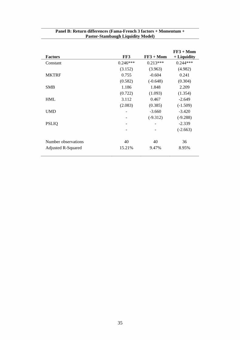
35

Panel B: Return differences (Fama-French 3 factors + Momentum +Pastor-Stambaugh Liquidity Model)

Factors FF3 FF3 + MomFF3 + Mom+ Liquidity

Constant 0.246*** 0.213*** 0.244***

(3.152) (3.963) (4.982)

MKTRF 0.755 -0.604 0.241

(0.582) (-0.648) (0.304)

SMB 1.186 1.848 2.209

(0.722) (1.093) (1.354)

HML 3.112 0.467 -2.649

(2.083) (0.385) (-1.509)

UMD - -3.660 -3.420

- (-9.312) (-9.288)

PSLIQ - - -2.339

- - (-2.663)

Number observations 40 40 36

Adjusted R-Squared 15.21% 9.47% 8.95%

36

Table IXRobustness Checks on Return Differences between Portfolios

This table shows the significance of the differences in returns between the non-reviser and reviser portfoliosfor different parameter choices as robustness checks. The monthly return differences are analysed using theFung-Hsieh 7 Factor model as a base model. Panel A shows the impact of using different levels ofsignificance before a revision is noted between vintages. So only absolute revisions greater than the toleranceparameter are treated as significant. These are in basis points i.e. 0.01%. Panel B shows the impact ofexcluding recent revisions near the vintage date. So only revisions at least k months of the vintage date areincluded. Newey-West heteroskedasticity and autocorrelation robust standard errors (with three lags) areused. Regression betas are shown with t-statistics shown in brackets beneath. Alpha significance is denotedby stars at 10% (*), 5% (**) and 1% (***) respectively.

Panel A: Significance of Revision (Fung-Hsieh 7 Factor Model )

Minimum Significance of Revisions

Factors 1 bp 10 bp 50 bp 100 bp

Constant 0.229*** 0.252*** 0.241*** 0.258***

(2.877) (3.043) (2.768) (2.741)

SP500 0.018 0.018 -0.001 -0.004

(1.422) (1.428) (-0.086) (-0.261)

SMB 0.025 0.023 0.011 0.016

(1.532) (1.260) (0.591) (0.720)

BOND10YR -0.288 -0.138 -0.062 0.114

(-1.049) (-0.498) (-0.199) (0.297)

CREDSPR -0.026 0.127 0.367 0.509

(-0.107) (0.482) (1.255) (1.380)

PTFSBD -0.288 -0.086 0.175 0.608

(-0.439) (-0.137) (0.249) (0.712)

PTFSFX 0.950 0.950 0.885 1.104

(1.763) (2.086) (1.929) (1.546)

PTFSCOM -1.471 -1.410 -1.266 -1.767

(-2.147) (-2.202) (-1.890) (-1.627)

Num. Observations 40 40 40 40

R-Squared 24.00% 19.21% 23.61% 30.40%

Adjusted R-Squared 7.38% 1.54% 6.90% 15.17%

37

Panel B: Recency of Revision (Fung-Hsieh 7 Factor Model )

Minimum Recency of Revisions

Factors k = 1 k > 3 k > 6 k > 12

Constant 0.229*** 0.284*** 0.301*** 0.247***

(2.877) (3.396) (3.459) (2.881)

SP500 0.018 -0.000 -0.009 -0.009

(1.422) (-0.024) (-0.673) (-0.679)

SMB 0.025 0.030 0.041 0.062

(1.532) (2.005) (2.276) (1.992)

BOND10YR -0.288 -0.313 -0.268 -0.334

(-1.049) (-1.212) (-1.069) (-1.257)

CREDSPR -0.026 -0.023 0.059 -0.004

(-0.107) (-0.119) (0.338) (-0.024)

PTFSBD -0.288 -0.232 -0.137 -0.073

(-0.439) (-0.338) (-0.189) (-0.092)

PTFSFX 0.950 0.910 0.856 1.366

(1.763) (1.637) (1.589) (1.969)

PTFSCOM -1.471 -1.017 -1.002 -1.934

(-2.147) (-1.509) (-1.509) (-2.253)

Num. Observations 40 40 40 40

R-Squared 24.00% 14.46% 18.53% 24.85%

Adjusted R-Squared 7.38% -4.25% 0.71% 8.41%

38

Table XRobustness Checks on Return Differences by Fund Characteristic

This table shows the results of a robustness check on the differences in returns between the non-reviser andreviser using the cross section of certain fund characteristics. The monthly return differences, split into above(Hi) and below (Lo) median groups for certain characteristics, are analysed using the Fung-Hsieh 7 Factormodel as a base model. The first characteristic, Rho1, splits the funds in the respective portfolios into theabove and below median lifetime first return autocorrelation, where the cross-sectional median is computedacross all funds reporting in the period. For example, the first column for Rho1 marked Hi compares thedifference in returns between non-reviser and reviser funds that are above the median lifetime Rho1 value.The next characteristic shows the funds split by the lockup period as at the last available vintage. Finally,Fund Size shows the fund split by AUM level in the prior period. Returns are equally weighted in portfolios.Newey-West heteroskedasticity and autocorrelation robust standard errors (with three lags) are used.Regression betas are shown with t-statistics shown in brackets beneath.

Characteristic

Rho1 Lockup Fund Size

Factors Hi Lo Hi Lo Hi Lo

Constant 0.283*** 0.111* 0.331*** 0.139* 0.207*** 0.220**

(3.479) (1.689) (3.646) (1.928) (2.746) (2.190)

SP500 0.042 0.008 0.070 -0.015 -0.014 -0.028

(3.898) (0.473) (11.591) (-0.685) (-0.980) (-1.035)

SMB 0.017 0.029 0.025 0.021 0.057 0.089

(1.043) (1.415) (1.705) (1.126) (2.651) (2.375)

BOND10YR -0.376 -0.463 0.043 -0.569 -0.768 -0.235

(-1.405) (-1.778) (0.151) (-1.727) (-2.797) (-0.962)

CREDSPR -0.134 -0.438 0.075 -0.436 -0.228 0.279

(-0.563) (-2.032) (0.254) (-1.921) (-1.518) (1.075)

PTFSBD -0.011 -1.291 0.199 -1.398 -0.549 -0.072

(-0.019) (-1.858) (0.318) (-1.852) (-0.815) (-0.087)

PTFSFX 0.954 1.322 1.070 0.769 -0.070 0.660

(1.764) (2.487) (1.990) (1.202) (-0.120) (0.847)

PTFSCOM -1.323 -2.449 -0.876 -2.355 0.043 -0.785

(-1.907) (-3.373) (-1.228) (-2.997) (0.070) (-0.651)

Num. Observations 40 40 40 40 40 40

R-Squared 46.75% 41.22% 59.61% 34.84% 29.52% 21.66%

Adjusted R-Squared 35.10% 28.36% 50.78% 20.58% 14.10% 4.52%

39

Figure IPortfolio Performance – Revisers and Non-Revisers

The figure shows the cumulative performance of the reviser and non-reviser portfolios. The non-reviserportfolio holds performance of funds that never revise between vintages plus the early records of fundsbefore they become revisers. For example, if a fund first revises at vintage v; its earlier performance will beincluded in the non-reviser portfolio as it had not yet been classified as a reviser. But once it joins the reviserportfolio it stays out of the non-reviser portfolio. The index is based to 100 at 31 December 2007, just beforethe second vintage starts. Returns are equally weighted in portfolios. Flows calculations use average assetsacross vintages.

Panel A. Revision Portfolio Indices: Returns

40

Panel B. Revision Portfolio Indices: Flows

41

Figure IICumulative Alpha

The figure plots cumulative alphas using the Fung-Hsieh 7 Factor model for the respective Reviser portfolioand Non-Reviser portfolio. The index is based to 100 at 31 December 2007, just before the second vintagestarts.

42

Figure IIITail Risk Percentiles for Reviser and Non-Reviser Portfolios

The figure shows the bottom decile tail statistics for the Reviser portfolio and Non-Reviser portfolio. Panel Ashows the empirical bottom decile for the portfolio fund returns using historical simulation. Panel B showsthe average return of those portfolio fund returns in this bottom decile as a measure of expected shortfall.

Panel A. Tail Risk Bottom Decile – Portfolio’s Fund Returns

43

Panel B. Tail Risk Average over Bottom Decile – Portfolio’s Fund Returns

44

Figure IVDifferences between “True” and Initial Returns

The figure shows the mean positive and negative return differences between the last expression of the returnat the most recent available vintage (denoted “True”) and the first time the return is expressed in a database(denoted Initial). Significant differences only are shown (so zero differences and minor differences due tochanges in expression of significant digits for the same return value are excluded). The vertical pink dashedlines are the points at which mean hedge fund returns in the universe are negative, and two standarddeviations below the time-series mean. The horizontal lines are two standard deviations of the positive andnegative revisions.

45

Figure VCumulative Differences between “True” and Initial Returns

The figure shows the cumulative average return differences between the last expression of the return at themost recent available vintage (denoted “True”) and the first time the return is expressed in a database(denoted Initial). Significant differences only are shown. The index is based to 100 at the time of the start ofthe return data, January 1994.

46

Figure VIPortfolio Performance – Revisers and Non-revisers Characteristic Checks

The figure shows the cumulative performance of the reviser and non-reviser portfolios, split into above andbelow median groups, for certain characteristics. Panel A splits the funds in the respective portfolios intothose above and below the median lifetime first return autocorrelation (Rho1) in each period, where thecross-sectional median is computed across all funds reporting in the period. For example, the reviser - HighRho1 portfolio plots cumulative mean returns for all funds that have revised at least once and are above themedian lifetime Rho1 level. Panel B shows the funds split by the lockup period as at the last availablevintage. Panel C shows the fund split by median AUM level in the prior period. The index is based to 100 at31 December 2007, just before the second vintage starts. Returns are equally weighted in portfolios.

Panel A: Revision Portfolio Indices: Returns split by Characteristic: Rho1

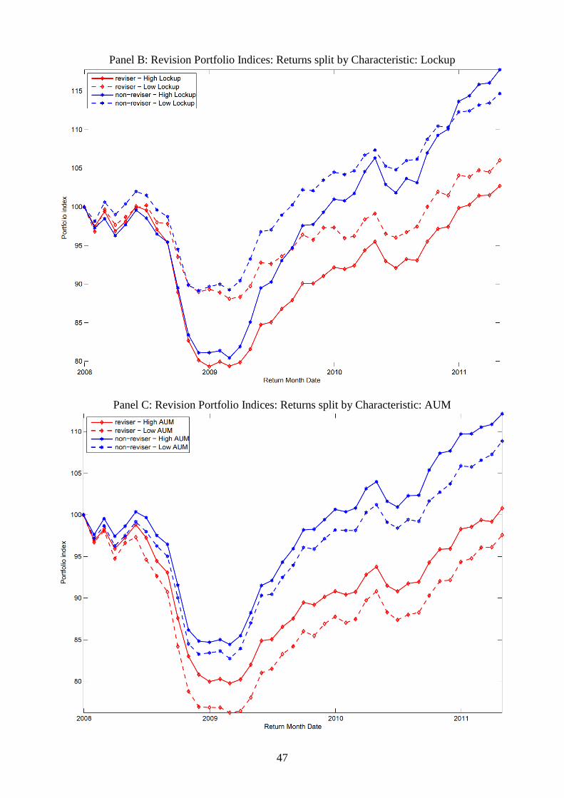
47

Panel B: Revision Portfolio Indices: Returns split by Characteristic: Lockup

Panel C: Revision Portfolio Indices: Returns split by Characteristic: AUM

the reliability of voluntary disclosures: evidence from...

Documents