THE RELATIVE VALUATION OF CAPS AND SWAPTIONS:

THEORY AND EMPIRICAL EVIDENCE

Francis A. LongstaffPedro Santa-Clara

Eduardo S. Schwartz∗

Initial version: August 1999.Current version: September 2000.

∗ The Anderson School at UCLA, Box 951481, Los Angeles, CA 90095-1481. Corre-sponding author’s email address: francis.longstaff@anderson.ucla.edu. We acknowl-edge the capable research assistance of Martin Dierker and Bing Han. We are gratefulfor the comments of seminar participants at Capital Management Sciences, ChaseManhattan Bank, Countrywide, Credit Suisse First Boston, Daiwa Securities, M.I.T,the Nippon Finance Association, the Norinchukin Bank, the Portuguese Finance Net-work meetings, Risk Magazine Conferences in Boston, London, and New York, Sa-lomon Smith Barney in London and New York, Simplex Capital, and Sumitomo Bank.We are particularly grateful for the comments and suggestions of Alan Brace, QiangDai, Yoshihiro Mikami, Joao Pedro Nunes, Soetojo Tanudjaja, Toshiki Yotsuzuka,an anonymous referee, and the editor, Rene Stulz. All errors are our responsibility.Copyright 2000.

ABSTRACT

Although traded as distinct products, caps and swaptions are linked byno-arbitrage relations through the correlation structure of interest rates.Using a string market model framework, we solve for the correlation ma-trix implied by the swaptions market and examine the relative valuationof caps and swaptions. The results indicate that swaption prices are gen-erated by four factors and that implied correlations are generally lowerthan historical correlations. We find evidence that long-dated swaptionsare priced inconsistently and that there were major distortions in theswaptions market during the hedge-fund crisis of late 1998. We also findthat cap prices periodically deviate significantly from the no-arbitragevalues implied by the swaptions market.

1. INTRODUCTION

The growth in interest-rate swaps during the past decade has led to the creationand rapid expansion of markets for two important types of swap-related derivatives:interest-rate caps and swaptions. These OTC derivatives are widely used by manyfirms to manage their interest-rate risk exposure and collectively represent the largestclass of fixed-income options in the financial markets. The International Swaps andDerivatives Association (ISDA) estimates that the total notional amount of caps andswaptions outstanding at the end of 1997 was over $4.9 trillion, which was more than300 times the $15 billion notional of all Chicago Board of Trade Treasury note andbond futures options combined.

Caps and swaptions are generally traded as separate products in the financial mar-kets, and the models used to value caps are typically different from those used tovalue swaptions. Furthermore, most Wall Street firms use a piecemeal approachin calibrating their models for caps and swaptions, making it difficult to evaluatewhether these derivatives are fairly priced relative to each other. Financial theory,however, implies no-arbitrage relations which must be satisfied by cap and swaptionprices. Specifically, a cap can be represented as a portfolio of options on individualforward rates. In contrast, a swaption can be viewed as an option on a portfolioof individual forward rates. Because of this, standard option pricing theory suchas Merton (1973) implies that the relation between cap and swaption prices, or be-tween different swaption prices, is driven primarily by the correlation structure ofthe forward rates. Given a unified valuation framework capturing these correlations,the no-arbitrage relations among cap and swaption prices can be tested directly.

This paper conducts an empirical analysis of the relative valuation of caps andswaptions using an extensive data set of interest-rate option prices. As the valuationframework, we use a string market model of the term structure of interest rateswhich blends the market-model framework of Brace, Gatarek, and Musiela (1997)and Jamshidian (1997) with the string-shock framework of Santa-Clara and Sornette(2000), Goldstein (2000), and Longstaff and Schwartz (2000). This approach hasthe important advantages of incorporating correlations directly into the model in asimple way and providing a unified framework for valuing fixed-income derivatives.The empirical approach taken in the paper consists of first solving for the covariancematrix implied by the market prices of all traded swaptions. This is the matrixequivalent of the familiar technique of solving for the implied volatility of an option.Once the implied covariance matrix has been identified, we can directly examine theimplications for the relative values of caps and swaptions.

The empirical results provide a number of interesting insights into the fixed-incomederivatives market. We find evidence of four statistically significant factors in thecovariance matrix implied from market swaption prices. This contrasts with resultsbased on historical covariance matrices which typically find only two to three factors,but is consistent with more recent evidence by Knez, Litterman, and Scheinkman

1

(1994). Our results indicate that the market considers factors that contribute littleto the unconditional volatility of term structure movements, but represent a majorsource of conditional volatility during periods of market stress. Our results alsoindicate that the correlations among forward rates implied from swaption pricestend to be lower than those observed historically.

We then examine the relative valuation of swaptions and find that most swaptionstend to be valued fairly relative to each other. The major exception is during thetwelve-week period immediately following the announcement in September 1998 ofmassive trading losses at Long Term Capital Management. During this turbulentperiod, there is strong evidence of significant distortions in the quoted prices of manyswaptions, a finding independently corroborated by interviews with many fixed-income derivatives traders. We also find that long-dated swaptions generally tendto be undervalued relative to other swaptions throughout the sample period.

Turning to the relative valuation of caps and swaptions, we find that the mediandifferences between model and market cap prices are close to zero. The distributionof differences, however, is skewed towards the right and all of the mean differences arepositive and significant. This suggests that caps are typically valued fairly relativeto swaptions, but that there are periodically large discrepancies between the twomarkets. This is particularly true during the hedge-fund crisis during late 1998.

Finally, we contrast the hedging performance of the string market model with thatof the standard Black model often used in practice. Despite using only four hedgingportfolios to hedge all of the swaptions in the sample, the string market modelperforms slightly better than the Black model which uses a different hedge portfoliofor each of the 34 swaptions in our sample.

The remainder of this paper is organized as follows. Section 2 provides a briefintroduction to cap and swaption markets. Section 3 describes the string marketmodel framework used to value interest-rate derivatives. Section 4 discusses the data.Section 5 presents the empirical results. Section 6 compares the implications of thestring model for fixed-income derivatives with those of the Black model. Section 7summarizes the results and makes concluding remarks.

2. THE CAPS AND SWAPTIONS MARKETS

This section provides a brief introduction to the caps and swaptions markets. Wefirst describe the characteristics of caps and explain how they are used in the financialmarkets. We then discuss the features of swaptions and their uses.

2.1 The Caps Market.

Many financial market participants enter into financial contracts in which they pay orreceive cash flows tied to some floating rate such as Libor. To hedge the risk created

2

by the variability of the floating rate, firms often enter into derivative contracts thatare essentially calls or puts on the level of the Libor rate. These types of derivativesare known as interest-rate caps and floors.

Specifically, a cap gives its holder a series of European call options or caplets on theLibor rate, where each caplet has the same strike price as the others, but a differentexpiration date.1 Typically, the expiration dates for the caplets are on the samecycle as the frequency of the underlying Libor rate. For example, a five-year capon three-month Libor struck at six percent represents a portfolio of 19 separatelyexercisable caplets with quarterly maturities ranging from 1/2 to five years, whereeach caplet has a strike price of .06.2 The cash flow associated with a caplet expiringat time T is (a/360)max(0, L(τ, T )−K) where a is the actual number of days duringthe period from τ to T , L(τ, T ) is the value at time τ of the Libor rate applicablefrom time τ to T , and K is the strike price. Note that while the cash flow on thiscaplet is received at time T , the Libor rate is determined at time τ , which meansthat there is no uncertainty about the cash flow from the caplet after Libor is set attime τ . The series of cash flows from the cap provides a hedge for an investor who ispaying Libor on a quarterly or semiannual floating-rate note, where each quarterlyor semiannual caplet hedges an individual floating coupon payment. In additionto caps, market participants often use interest-rate floors. These are similar tocaps, except that the cash flow from an individual floorlet with expiration date Tis (a/360)max(0, K −L(τ, T )). Thus, floors are essentially a series of European putoptions on the Libor rate. The market for interest-rate caps and floors is genericallytermed the caps market.

Market prices for caps and floors are universally quoted relative to the Black (1976)model. Specifically, letD(t, T ) denote the value at time t of a discount bond maturingat time T , and let F (t, τ, T ) denote the value at time t for the Libor forward rateapplicable to the period from time τ to T . Since L(τ, T ) = F (τ, τ, T ), a caplet can beviewed as an option on an individual Libor forward rate. Applying the Black modelto this forward rate results in the following closed-form expression for the time-zerovalue of a caplet with expiration date T

D(0, T )a

360

hF (0, τ, T )N(d)−K N

¡d−

√σ2τ/2

¢i, (1)

where

d =ln¡F (0, τ, T )/K

¢+√σ2τ/2√

σ2τ

1For many currencies, the market convention is for the cap to be on the three-monthLibor rate. In some markets, however, caps may be on the six-month Libor rate.For example, Yen caps with maturities greater than one year are usually on thesix-month Libor rate.2The standard market convention is to omit the first caplet since the cash flow fromthis caplet is set at time t = 0 and is not stochastic.

3

and

F (0, τ, T ) =360

a

µD(0, τ)

D(0, T )− 1¶

and where σ is the volatility of changes in the logarithm of the forward rate. Withthis closed-form solution, the price of a cap is given by summing the values of theconstituent caplets. Thus, a cap is simply a portfolio of individual options, each on adifferent forward Libor rate. The market convention is to quote cap prices in termsof the implied value of σ which sets the Black model price equal to the market price.Note that the convention of quoting cap prices in terms of the implied volatility fromthe Black model does not necessarily mean that market participants view the Blackmodel as the most appropriate model for caps. Rather, implied volatilities fromthe Black model are simply a more convenient way of quoting prices, since impliedvolatilities tend to be more stable over time than the actual dollar price at which acap would be traded.

2.2 The Swaptions Market.

The underlying instrument for a swaption is an interest rate swap. In a standardswap, two counterparties agree to exchange a stream of cash flows over some specifiedperiod of time. One counterparty receives a fixed annuity and pays the other astream of floating cash flows tied to the three-month Libor rate. Counterparties areidentified as either receiving fixed or paying fixed in the swap. Although principalis not exchanged at the end of a swap, it is often more intuitive to think of a swapas involving a mutual exchange of $1 at the end of the swap. From this perspective,the cash flows from the fixed leg are identical to those from a bond with coupon rateequal to the swap rate, while the cash flows from the floating leg are identical tothose from a floating rate note. Thus, a swap can be viewed as exchanging a fixedrate coupon bond for a floating rate note.3

At the time a swap is initiated, the coupon rate on the fixed leg of the swap isspecified. Intuitively, this rate is chosen to make the present value of the fixedleg equal to the present value of the floating leg. To illustrate how the fixed rate isdetermined, designate the current date as time zero and the final maturity date of theswap as time T . The fixed rate at which a new swap with maturity T can be executedis known as the constant maturity swap rate and we denote it by FSR(0, 0, T ), wherethe first argument refers to time zero, the second argument denotes the start dateof the swap which is time zero for a standard swap, and T is the final maturity dateof the swap. Once a swap is executed, then fixed payments of FSR(0, 0, T )/2 are

3For discussions about the economic role that interest-rate swaps play in finan-cial markets, see Bicksler and Chen (1986), Turnbull (1987), Smith, Smithson, andWakeman (1988), Wall and Pringle (1989), Macfarlane, Ross, and Showers (1991),Sundaresan (1991), Litzenberger (1992), Sun, Sundaresan, and Wang (1993), andGupta and Subrahmanyam (2000).

4

made semiannually at times .50, 1.00, 1.50, . . . , T − .50, and T . Floating paymentsare made quarterly at times .25, .50, .75, . . . , T − .25, and T and are equal to a/360times the three-month Libor rate at the beginning of the quarter, where a is theactual number of days during the quarter. This feature is termed setting in advanceand paying in arrears. Abstracting from credit issues, a floating rate note payingthree-month Libor quarterly must be worth par at each quarterly Libor reset date.Since the initial value of a swap is zero, the initial value of the fixed leg must alsobe worth par. Setting the time-zero values of the two legs equal to each other andsolving for the swap rate gives

FSR(0, 0, T ) = 2

∙1−D(0, T )A(0, 0, T )

¸, (2)

where A(0, 0, T ) =P2T

i=1D(0, i/2) is the present value of an annuity with first pay-ment six months after the start date and final payment at time T . Swap rates arecontinuously available from a wide variety of sources for standard swap maturitiessuch as 2, 3, 4, 5, 7, 10, 12, 15, 20, 25, and 30 years.

For many swaptions, the underlying swap has a forward start date. In a forwardswap with a start date of τ , fixed payments are made at time τ + .50, τ + 1.00, τ +1.50, . . . , T − .50, and T and floating rate payments are made at times τ + .25, τ +.50, τ+.75, . . . , T−.25, and T . At the start date τ , the value of the floating leg equalspar. Discounting this time-τ value back to time zero implies that the time-zero valueof the floating cash flows is D(0, τ). Since the forward swap has a time-zero value ofzero, the time-zero value of the fixed leg must also equal D(0, τ). This implies thatthe forward swap rate FSR(0, τ, T ) must satisfy

FSR(0, τ, T ) = 2

∙D(0, τ)−D(0, T )

A(0, τ, T )

¸. (3)

After a swap is executed, the coupon rate on the fixed leg may no longer equal thecurrent market swap rate and the value of the swap can deviate from zero. LetV (t, τ, T, c) be the value at time t to the counterparty receiving fixed in a swap withforward start date τ ≥ t and final maturity date T , where the coupon rate on thefixed leg is c. The value of this forward swap is given by

V (t, τ, T, c) =c

2

2(T−τ)Xi=1

D(t, τ + i/2) +D(t, T )−D(t, τ), (4)

where the first two terms in this expression represent the value of the fixed leg of theswap, and the third term is the present value of the floating leg which will be worthpar at time τ . For t > τ , the swap no longer has a forward start date and the valueof the swap on semiannual fixed coupon payment dates is given by the expression

5

V (t, τ, T, c) =c

2

2(T−t)Xi=1

D(t, τ + i/2) +D(t, T )− 1. (5)

Note that in either case, the value of the swap is just a linear combination of zero-coupon bond prices.

Swaptions or swap options allow their holder to enter into a swap with a prespecifiedfixed coupon rate, or to cancel an existing swap. Intuitively, swaptions can alsobe viewed as calls or puts on coupon bonds. Natural end users of swaptions aregovernment agencies and firms coming to the capital markets to borrow funds. Theseentities use swaptions for the same reasons many firms issue callable or puttabledebt–to cancel a swap with an above-market coupon rate or to enter into a newswap at a below-market coupon rate.

There are two basic types of European swaptions.4 The first is the option to enter aswap and receive fixed. For example, let τ be the expiration date of the swaption, cbe the coupon rate on the swap, and T be the final maturity date on the swap. Theholder of this option has the right at time τ to enter into a swap with a remainingterm of T − τ , and receive the fixed annuity of c. Since the value of the floatingleg will be par at time τ , this option is equivalent to a call option on a bond witha coupon rate of c and a remaining maturity of T − τ where the strike price of thecall is $1. This option is generally called a τ into T − τ receivers swaption, where τis the maturity of the option and T − τ is the tenor of the underlying swap. Thisswaption is also known as a τ by T receivers swaption. Note that if the option holderis paying fixed at rate c in a swap with a final maturity date of T , then exercisingthis option has the effect of canceling the original swap at time τ since the two fixedand two floating legs cancel each other out. Observe, however, that when the optionis used to cancel the swap at time τ , the current fixed for floating coupon exchangeis made first.

The second type of swaption is the option to enter a swap and pay fixed, and thecash flows associated with this option parallel those described above. An optionwhich gives the option holder the right to enter into a swap at time τ with finalmaturity date at time T and pay fixed is generally termed a τ into T − τ or a τby T payers swaption. Again, this option is equivalent to a put option on a couponbond where the strike price is the value of the floating leg at time τ of $1. A τ byT payers swaption can be used to cancel an existing swap with final maturity dateat time T where the option holder is receiving fixed at rate c.

From the symmetry of the European payoff functions, it is easily shown that a longposition in a τ by T receivers swaption and a short position in a τ by T payers

4For a discussion of the characteristics of American-style swaptions, see Longstaff,Santa-Clara, and Schwartz (2000).

6

swaption with the same coupon has the same payoff as receiving fixed in a forwardswap with start date τ and coupon rate c. A standard no-arbitrage argument givesthe receivers/payers parity result that at time t, 0 ≤ t ≤ τ , the value of the forwardswap must equal the value of the receivers swaption minus the value of the payersswaption. When the coupon rate c equals the forward swap rate FSR(t, τ, T ), theforward swap is worth zero and the receivers and payers swaptions have identicalvalues. In this case, the swaptions are said to be at the money forward.

As in the caps markets, the convention in the swaptions market is to quote pricesin terms of their implied volatility relative to a standard pricing model. In swaptionmarkets, prices are quoted as implied volatilities relative to the Black (1976) modelas applied to the forward swap rate. Again, this does not mean that the marketviews this model as the most accurate model for swaptions. To illustrate how pricesare quoted in the swaptions market, consider a τ by T European payers swaptionwhere the fixed coupon rate equals c. Under the assumption that the forward swaprate follows a lognormal process under the annuity measure (the measure where thevalue of the annuity A(t, τ, T ) is used as the numeraire), the Black model impliesthat the value of this swaption at time zero is

1

2A(0, τ, T )

hFSR(0, τ, T )N(d)− cN(d− σ√τ)

i, (6)

where

d =ln(FSR(0, τ, T )/c) + σ2τ/2

σ√τ

,

whereN(·) is again the cumulative standard normal distribution function and σ is thevolatility of the logarithm of the forward swap rate. The value of the correspondingreceivers swaption is given from the receivers/payers parity result. In the specialcase where the swaption is at-the-money forward, c = FSR(0, τ, T ) and equation (6)reduces to

¡D(0, τ)−D(0, T )¢ £2N ¡σ√τ/2¢− 1¤ . (7)

Since this receivers swaption is at the money forward, the value of the correspondingpayers swaption is identical. When an at-the-money-forward swaption is quotedat an implied volatility of σ, the actual price that is paid by the purchaser of theswaption is given by substituting σ into equation (7).5

5Smith (1991) describes the application of the Black (1976) model to Europeanswaptions. Jamshidian (1997), Brace, Gatarek, and Musiela (1997), and othersdemonstrate that the Black model for swaptions can be derived within an internally-consistent no-arbitrage model of the term structure in which the numeraire is thevalue of an annuity.

7

In the previous section, we showed that caps are simple portfolios of options on indi-vidual forward rates. In contrast, swaptions can be viewed as options on portfoliosof forward rates. To see this, recall that a swaption is an option on the forward swaprate in the Black (1976) model. Furthermore, forward swap rates can be expressed asnearly linear functions of individual forward rates, where the weights are related tothe durations of the cash flows from the fixed leg of the swap.6 From this, it followsthat the swaption can be thought of as an option on a linear combination or portfo-lio of forward rates. Merton (1973) presents a number of no-arbitrage propositionsincluding the well-known result that the value of an option on a portfolio must beless than or equal to that of a corresponding portfolio of options. This inequality isstrict if the assets underlying the individual options are not perfectly correlated. Al-though the forward swap rate is only approximately linear in the individual forwardrates, the key implication of the Merton result, namely that the relative value of aportfolio of options and an option on a portfolio is determined by the correlationsbetween the underlying assets, is directly applicable to caps and swaptions. This keyimplication motivates many of the empirical tests later in the paper. In particular,we solve for the correlation matrix among forwards implied by a set of swaptionprices, and then examine the extent to which other fixed-income options satisfy theno-arbitrage restrictions imposed by the correlation structure of forwards.

Finally, while both caps and swaptions are quoted in terms of the Black (1976) model,it should be recognized that the Black model is being actually used in different waysin these markets. In particular, the caps market uses the forward short-term Liborrate as the underlying state variable in the Black model, while the swaptions marketuses longer-term forward swap rates. Since forward swap rates are nearly linear inindividual forward rates, the lognormality assumption implicit in the Black modelcannot hold simultaneously for both individual forward rates and forward swap rates,since a linear combination of lognormal variates is not lognormal. This is the sense inwhich the two markets use different models; the inputs used in the Black model differacross the two markets. In addition, since the volatilities used in the Black modelare for fundamentally different rates, direct comparisons between the quoted impliedvolatilities of caps and swaptions are invalid. This has important implications forthe risk management of portfolios of caps and swaptions.

3. THE VALUATION FRAMEWORK

In this section, we develop a general string market model for valuing fixed-incomederivatives such as caps and swaptions. We then describe how to invert the modelto solve for the implied covariance matrix that best fits observed market prices.

6This well-known rule of thumb or approximation can be obtained by differentiatingthe expression for the forward swap rate in equation (3) with respect to either spotor forward rates. For example, see Fabozzi (1993, Chapter 5).

8

3.1 The String Market Model.

In a series of recent papers, Jamshidian (1997), Brace, Gatarek, and Musiela (1997),and others develop term structure models in which either Libor forward rates orforward swap rates are taken to be fundamental and their dynamics modeled di-rectly using a Heath, Jarrow, and Morton (1992) framework. This class of mod-els is often referred to as market models since they are based on the forwards ofobservable term rates in the market rather than on instantaneous forward rates.This approach has the advantage of solving some technical problems associated withcontinuously-compounded lognormal rates as well as paralleling the standard practi-tioner approach of basing models on term rates. Libor-based and swap-based marketmodels have been applied to a variety of interest-rate derivative valuation problems.Because the structure of these models is closely related to that of the Heath, Jarrow,and Morton framework, they share many of the same calibration issues and havetypically only been implemented with a small number of factors.

In another recent literature, Kennedy (1994, 1997), Santa-Clara and Sornette (2000),Goldstein (2000), and Longstaff and Schwartz (2000) model the evolution of the termstructure as a stochastic string. In this approach, each point along the term structureis a distinct random variable with its own dynamics, but which may be correlatedwith the other points along the term structure. Thus, string models are inherentlyhigh-dimensional models. Surprisingly, however, string models can actually be mucheasier to calibrate than models with fewer factors. The reason for this is that stringmodels are directly parameterized by the correlation function for the points along thestring. This direct approach is generally much more parsimonious than the standardapproach of parameterizing the elements of a matrix of diffusion coefficients. Theadvantages of the string model approach to parameterization become increasinglyimportant as the number of factors driving the term structure increases. Santa-Claraand Sornette show that the string model approach generalizes the Heath, Jarrow,and Morton (1992) framework for instantaneous forward rates while preserving itsintuitive structure and appeal.

In this paper, we blend the market model setup with the string model approachof calibration to develop a valuation framework for fixed-income derivatives. Thisapproach has the advantage of allowing us to develop the model in terms of theforward Libor rates which underlie the prices of caps and swaptions. At the sametime, this approach makes it possible to directly model the correlation structureamong Libor forwards in a simple way even when there are a large number of factors.Capturing the correlation structure is particularly important in this study; recallfrom earlier discussion that the correlation structure among forwards plays a centralrole in determining the relative valuation of caps and swaptions. We designate thisvaluation framework the string market model (SMM).

In this model, we take the Libor forward rates out to ten years Fi ≡ F (t, Ti, Ti +1/2), Ti = i/2, i = 1, 2, . . . , 19, to be the fundamental variables driving the termstructure. Similarly to Black (1976), we assume that the risk-neutral dynamics for

9

each forward rate are given by

dFi = αi Fi dt+ σi Fi dZi, (8)

where αi is an unspecified drift function, σi is a deterministic volatility function,dZi is a standard Brownian motion specific to this particular forward rate, andt ≤ Ti.

7 Note that while each forward rate has its own dZi term, these dZi termsare correlated across forwards. The correlation of the Brownian motions togetherwith the volatility functions determine the covariance matrix of forwards Σ. This isdifferent from traditional implementations of multi-factor models which use severaluncorrelated Brownian motions to shock each forward rate. This seemingly minordistinction actually has a number of important implications for the estimation ofmodel parameters from market data.

To model the covariance structure among forwards in a parsimonious but economi-cally sensible way, we make the assumption that the covariance between dFi/Fi anddFj/Fj is time homogeneous in the sense that it depends only on Ti− t and Tj − t.8Furthermore, since our objective is to apply the model to swaps which make fixedpayments semiannually, we make the simplifying assumption that these covariancesare constant over six-month intervals. With these assumptions, the problem of cap-turing the covariance structure among forwards reduces to specifying a 19 by 19time-homogenous covariance matrix Σ.

One of the key differences between this string market model and traditional multi-factor models is that our approach allows the parameters of the model to be uniquelyidentified frommarket data. For example, if there areN forward rates, the covariancematrix Σ has only N(N + 1)/2 distinct parameters. Thus, market prices of fixed-income derivatives contain information on at most N(N + 1)/2 covariances, and nomore than N(N +1)/2 parameters can be uniquely identified from the market data.Since the string market model is parameterized by Σ, the parameters of the modelare econometrically identified. In contrast, a typical implementation with constantcoefficients of a traditional N-factor model of the form

7We assume that the initial value of Fi is positive and that the unspecified αi termsare such that standard conditions guaranteeing the existence and uniqueness of astrong solution to equation (8) are satisfied. These conditions are described inKaratzas and Shreve (1988, Chapter 5). In addition, we assume that αi is suchthat Fi is non-negative for all t ≤ Ti.8Although the assumption of time homogeneity imposes additional structure on themodel, it has the advantage of being more consistent with traditional dynamicterm structure models in which interest rates are determined by the fundamentalstate of the economy. In addition, time homogeneity facilitates econometric estima-tion because of the stationarity of the model’s specification. For discussions of theadvantages of time-homogeneous models, see Andersen and Andreasen (2000) andLongstaff, Santa-Clara, and Schwartz (2000).

10

dFi = αiFidt+ σi1FidZ1 + σi2FidZ2 + . . .+ σiNFidZN , (9)

would require N parameters for each of the N forwards, resulting in a total of N2

parameters. Given that there are only N(N + 1)/2 < N2 separate covariancesamong the forwards, the general specification in equation (9) cannot be identifiedusing market information unless additional structure is placed on the model. Similarproblems also occur when there are fewer factors than forwards. By specifying thecovariance or correlation matrix among forwards directly, the string market modelavoids these identification problems. String models also have the advantage of beingmore parsimonious. For example, up toN×K parameters would be needed to specifya traditional K-factor model. In contrast, only K(K + 1)/2 parameters would beneeded to specify a string market model with rank K.9

Although the string is specified in terms of the forward Libor rates, it is much moreefficient to implement the model using discount bond prices. By definition,

Fi =360

a

∙D(t, Ti)

D(t, Ti + 1/2)− 1¸. (10)

Thus, the forward rates Fi can all be expressed as functions of the vector of discountbond prices with maturities .50, 1, . . . , 10. Conversely, these discount bond pricescan be expressed as functions of the string of forward rates, assuming that standardinvertibility conditions are satisfied.10 Applying Ito’s Lemma to the vector D ofdiscount bond prices gives

dD = r D dt+ J−1 σ F dZ, (11)

where r is the spot rate, σ F dZ is the vector formed by stacking the individualterms σi(t, Ti) Fi dZi in the forward rate dynamics in equation (8), and J

−1 is theinverse of the Jacobian matrix for the mapping from discount bond prices to forwardrates. Since each forward depends only on two discount bond prices, this Jacobianmatrix has the following simple banded diagonal form.11

9These types of identification problems parallel those which occur in general affineterm structure models. The specification and identification issues associated withaffine term structure models are discussed in an important recent paper by Dai andSingleton (2000).

10The primary condition is that the determinant of the Jacobian matrix for the map-ping from discount bond prices to forward swap rates be non-zero. If this conditionis satisfied, local invertibility is implied by the Inverse Function Theorem.

11For notational simplicity, discount bonds are expressed as functions of their matu-rity date in the Jacobian matrix. The Jacobian matrix represents the derivative ofthe 19 forwards F.50, F1.00, F1.50, . . . , F9.50 with respect to the discount bond prices

11

J =

− D(.50)D2(1.00) 0 0 . . . 0 0 0

1D(1.50) − D(1.00)

D2(1.50) 0 . . . 0 0 0

0 1D(2.00) − D(1.50)

D2(2.00) . . . 0 0 0

......

.... . .

......

...

0 0 0 . . . 1D(9.50) − D(9.00)

D2(9.50) 0

0 0 0 . . . 0 1D(10.00) − D(9.50)

D2(10.00)

It is important to observe that the drift term rD in equation (11) does not dependon the drift term αi in equation (8). The reason for this is that discount bondsare traded assets in this complete markets setting and their instantaneous expectedreturn is equal to the spot rate under the risk-neutral measure.12 Thus, this stringmarket model formulation has the advantage of allowing us to avoid specifying thecomplicated drift term αi, making the model numerically easier to work with thanformulations based entirely on forward rates. Again, since our objective is a discrete-time implementation of this model, we make the simplifying assumption that r equalsthe yield on the shortest-maturity bond at each time period.13

The dynamics forD in equation (11) provide a complete specification of the evolutionof the term structure. This string market model is arbitrage free in the sense that itfits the initial term structure exactly and the expected rate of return on all discountbonds equals the spot rate under the risk-neutral pricing measure. Furthermore, themodel allows each point along the curve to be a separate factor, but also allows for

D(1.00), D(1.50), D(2.00), . . . , D(10.00). Since σ(Ti − t) = 0 for Ti ≤ .50, D(.50)is not stochastic and does not affect the diffusion term in equation (11).

12The bond market is complete in the sense that there are as many traded bondsas there are sources of risk. Thus, while no discount bond is a redundant asset, themarket is complete and all fixed income derivatives can be priced under a risk-neutralmeasure in which the expected returns on all bonds equals the riskless rate. For adiscussion of this point, see Santa-Clara and Sornette (2000).

13Extensive numerical tests indicate that this discretization assumption has littleeffect on the results; we find that this approach gives values for European swaptionsthat are virtually identical to those implied by their closed-form solutions.

12

a general correlation structure through Σ. To complete the parameterization of themodel, we need only specify Σ in a way that matches the market or the historicalbehavior of forward rates.

3.2 Implied Covariance Matrices.

Rather than specifying the covariance matrix Σ exogenously, our approach is tosolve for the implied matrix Σ that best fits the observed market prices of someset of market data. Specifically, we imply the covariance matrix from the set of allobserved European swaption prices.

In solving for the implied covariance matrix, it is important to note that a covari-ance matrix must be positive definite (or at least positive semidefinite) to be welldefined. This means that care must be taken in designing the algorithm by which thecovariance matrix is implied from the data to insure than this condition is satisfied.Standard results in linear algebra imply that a matrix is positive definite if, and onlyif, the eigenvalues of the matrix are all positive.14

Motivated by this necessary and sufficient condition, we use the following procedureto specify the implied covariance matrix. First, we estimate the historical correlationmatrix of percentage changes in forward rates H from a time series of forward ratestaken from a five-year period prior to the beginning of the sample period used inour study.15 We then decompose the historical correlation matrix into its spectralrepresentation H = UΛU 0, where U is the matrix of eigenvectors and Λ is a diagonalmatrix of eigenvalues. Finally, we make the identifying assumption that the impliedcovariance matrix is of the form Σ = UΨU 0, where Ψ is a diagonal matrix with non-negative elements. This assumption places an intuitive structure on the space ofadmissible implied covariance matrices.16 Specifically, if the eigenvectors are viewedas factors, then this assumption is equivalent to assuming that the factors that gen-erate the historical correlation matrix also generate the implied covariance matrix,but that the implied variances of these factors may differ from their historical values.Viewed this way, the identification assumption is simply the economically intuitiverequirement that the market prices swaptions based on the factors which drive termstructure movements. Extensive numerical tests suggest that virtually any realisticimplied correlation matrix can be closely approximated by this representation.17

14For example, see Noble and Daniel (1977).

15We implement this procedure using the historical correlation matrix rather thanthe covariance matrix to simplify the scaling of implied eigenvalues. We have alsoimplemented this procedure using the historical covariance matrix. Not surprisingly,the eigenvectors from the historical covariance matrix are very similar to those ob-tained from the historical correlation matrix.16This assumption is equivalent to requiring that the historical correlation matrix Hand the implied covariance matrix Σ commute, that is, HΣ = ΣH. We are gratefulto Bing Han for this observation.

17We note that there are alternative ways of specifying the correlation matrix. For

13

Given this specification, the problem of finding the implied covariance matrix reducesto solving for the implied eigenvalues along the main diagonal of Ψ that best fit themarket data. Since there are typically far more swaptions than eigenvalues, we solvefor the implied eigenvalues by standard numerical optimization where the objectivefunction is the root mean squared error (RMSE) of the percentage differences be-tween the market price and the model price, taken over all swaptions. Specifically,for a given choice of the elements of the diagonal matrix Ψ, we form the estimatedcovariance matrix UΨU 0 and then simulate 2,000 paths of the vector of discountbond prices using the string market model dynamics in equation (11). In simulatingcorrelated Brownian motions, we use antithetic variates to reduce simulation noise.The time homogeneity of the model is implemented in the following way. Duringthe first six-month simulation interval, the full 19 by 19 versions of the matrices Σand J are used to simulate the dynamics of the 19 forward rates. After six months,however, the first forward becomes the spot rate, leaving only 18 forward rates tosimulate during the second six month period. Because of the time homogeneity ofthe model, the relevant 18 by 18 covariance matrix is given by taking the first 18rows and columns of Σ; the last row and column is dropped from the covariancematrix Σ. Similarly, the first row and column are dropped from the Jacobian sincethey involve derivatives with respect to the first forward which has now become thespot rate. This process is repeated until the last six-month period when only thefinal forward rate remains to be simulated.

Using the paths generated, we then value the individual at-the-money-forward Eu-ropean swaptions by simulation and evaluate the RMSE. In simulating the prices ofswaptions, we use the following procedure. First, recall that since we simulate theevolution of the full vector of discount bond prices of all maturities ranging up to10 years, these bond values are available at the expiration date τ of the swaptionfor each of the simulated paths of the term structure. From these discount bondprices at time τ , we can calculate the value of the underlying swap for each path.Specifically, the value of the swap V (τ, τ, T, c) at time τ is given by the expression

V (τ, τ, T, c) =c

2

2(T−τ)Xi=1

D(τ, τ + i/2) +D(τ, T )− 1, (12)

example, Rebonato (1999) independently offers a method to construct correlationmatrices among forward rates. In the context of our framework, however, Rebonato’sapproach would require optimizing over a large number of parameters (e.g. in a four-factor model, his approach would require optimization over a set of 19× (4−1) = 57parameters) and is computationally infeasible. We also explored alternative waysof specifying the implied covariance matrix. For example, we examined a variety ofspecifications where the covariance between the i-th and j-th forwards is of the formea+bTiea+bTje−λ|Ti−Tj |, where a, b, and λ are calibrated to best fit swaption pricesbased on a RMSE criterion. These and other similar types of specifications generallyperformed poorly in terms of their RMSEs relative to the specification used in thispaper.

14

where c is the fixed coupon rate of the swap which is equal to the forward swap rateFSR(0, τ, T ) defined by equation (3). Thus, the value of the underlying swap at theexpiration date τ of the swaption is easily calculated using the vector of discountbond prices. Once the value of the underlying swap at time τ is determined, thecash flow from the swaption at time τ is simply max(0, V (τ, τ, T, c)) for a receiversswaption and max(0,−V (τ, τ, T, c)) for a payers swaption. For each path, we thendiscount the cash flow from the option by multiplying by the compounded money-market factor

Q2τ−1i=0 D(i, i + 1/2). Finally, we average the discounted cash flows

over all paths. Since at-the-money-forward receivers and payers swaptions have thesame value, we use the average of the simulated receivers and payers swaptions asthe simulated value of the swaption.

We iterate this entire process over different choices of the eigenvalues until conver-gence is obtained, using the same seed for the random number generator at eachiteration to preserve the differentiability of the objective function with respect tothe eigenvalue. Although 19 implied eigenvalues are required for the covariance ma-trix Σ to be of full rank, implied covariance matrices of lower rank can easily benested in this specification by solving for the first N eigenvalues and then settingthe remaining 19−N equal to zero.18

4. THE DATA

In conducting this study, we use three types of data: Libor and swap data defining theterm structure of interest rates, market implied volatilities for European swaptions,and market implied volatilities for Libor interest-rate caps. Together with the termstructure data, these implied volatilities define the market prices of swaptions andcaps. The source of all data is the Bloomberg system which collects and aggregatesmarket quotations from a number of brokers and dealers in the OTC swap andfixed-income derivatives market.

18Although the numerical optimization is conceptually straightforward, there are anumber of ways in which the search algorithm can be accelerated. For example,a least squares algorithm similar to Longstaff and Schwartz (2000) can be used toapproximate forward swap rates as linear functions of the individual forward rates.Given a covariance matrix, this linear approximation then implies closed-form ex-pressions for the variance of individual forward swap rates at the expiration dates ofthe swaptions, which can then be used to provide a closed-form approximation to thevalue of the swaption. This closed-form approximation can then be corrected for biasby an iterative process of comparing the simulated values given by the string marketmodel to those implied by this approximation, and then adjusting the approxima-tion. The implied eigenvalues can then be determined by optimizing the closed-formapproximation rather than having to resimulate paths of the term structure at eachiteration. With this type of algorithm, solving for the implied eigenvalues typicallytakes less than 10 seconds using a 750 MHz Pentium III processor.

15

The term structure data consists of weekly observations (Friday closing) for the six-month and one-year Libor rates as well as midmarket two-year, three-year, four-year,five-year, seven-year and ten-year par swap rates for the period from January 17,1992 to July 2, 1999. These maturities are the standard maturities for which swaprates are quoted in the market. From these rates, we solve for the term structureof six-month Libor forward rates out to ten years in the following way. We firstuse the six-month and one-year Libor rates to solve for the six-month and one-year par rates. We then use a standard cubic spline algorithm to interpolate thepar curve at semiannual intervals. Finally, we solve for six-month forward rates bybootstrapping the interpolated par curve.19 Table 1 reports summary statistics forthe Libor forward rates for the in-sample period from January 24, 1997 to July 2,1999. The term structures of Libor forward rates from this period are also graphedin Figure 1. The term structure data for the five-year ex-ante period from January17, 1992 to January 17, 1997 is used to estimate the historical correlation matrix Hfrom which the eigenvectors used in solving for the implied covariance matrices aredetermined. This ex-ante correlation matrix is shown in Table 2; all of the in-sampleresults are based on this ex-ante correlation matrix. Note that the correlationsare generally smooth monotonically-decreasing functions of the distance betweenforward rates. One interesting exception is the correlation between the first andsecond forwards; the first two forwards display a significant amount of independentvariation, hinting at money-market factors not present in longer-term forward rates.

The swaption data consists of weekly midmarket implied volatilities for 34 at-the-money-forward European swaptions for the in-sample period from January 24, 1997to July 2, 1999. These 34 swaptions represent all of the standard quoted τ byT European swaption structures where the final maturity date of the underlyingswap is less than or equal to ten years, T ≤ 10. As described earlier, the marketconvention is to quote swaption prices in terms of their implied volatility relativeto the Black (1976) model for at-the-money-forward European swaptions given inequation (7); the market prices of these swaptions are given by substituting theimplied volatilities into the Black model. Table 3 provides summary statistics forthe implied volatilities. Figure 2 graphs the implied volatilities over time; Figure 3shows a number of examples of the shape of the swaption implied volatility surfaceat different points in time during the sample period.

Observe that there is a significant spike in these implied volatilities during the Fall of1998. This spike coincides with the hedge-fund crisis precipitated by the announce-ment in early September 1998 of massive trading losses by Long Term Capital Man-agement (LTCM). The sudden threat to the solvency of LTCM, which had beenwidely viewed as a premier client by many Wall Street firms, created a near panic in

19Following the market convention, we discount cash flows using the swap curve asif it were the riskless term structure. Since the cash flows from both legs of a swapare discounted using this curve, however, this convention has little or no effect onvaluation results.

16

the financial markets. In the subsequent weeks, a number of other highly-leveragedhedge funds also announced that they had experienced large trading losses on posi-tions similar to those held by LTCM. Examples of these funds included ConvergenceCapital Management, Ellington Capital Management, D. E. Shaw & Co., and MKPCapital Management. In an effort to stabilize the market, the Federal Reserve Bankof New York persuaded a consortium of 16 investment and commercial banks toinject $3.6 billion into LTCM in exchange for virtually all of the remaining equityin the fund. The prompt action by the Federal Reserve, announced to the marketson September 24, 1998, allowed LTCM to avoid insolvency and reduced the pressureon the fund to unwind trading positions at illiquid fire-sale prices, which would haveexacerbated the problems at other hedge funds to which the consortium membershad considerable risk exposure.

The interest-rate cap data consists of weekly midmarket implied volatilities for two-year, three-year, four-year, five-year, seven-year, and ten-year caps for the sameperiod as for the swaptions data, January 24, 1997 to July 2, 1999. By marketconvention, the strike price of a T -year cap is simply the T -year swap rate. Toparallel the features of swaptions and to simplify the analysis, we assume that capsare on the six-month Libor rate rather than the three-month rate.20 The marketprices of caps are then given by substituting the implied volatility into the Blackmodel (1976) given in equation (1), where T − τ = 1/2. Table 4 presents summarystatistics for the market cap volatilities during the sample period. The impliedvolatilities display a time series pattern similar to those observed for swaptions.Figure 4 also graphs the time series of cap volatilities.

5. THE EMPIRICAL RESULTS

In this section, we report the empirical results from the study. First, we examinehow many implied factors are required to explain the market prices of swaptions. Wethen study the relative valuation of swaptions in the string market model. Finally,we examine the relative valuation of both caps and swaptions in the string marketmodel.

5.1 How Many Implied Factors?

Many researchers have studied the question of how many factors or principal com-ponents are needed to capture the historical variation in the term structure. Forexample, recent papers by Litterman and Scheinkman (1991) and others find that

20This assumption is relatively innocuous. We have spoken with several caps dealerswho indicated that the implied volatilities for caps on six-month Libor would typi-cally be equal to or perhaps an eighth to a quarter below the implied volatility fora cap on three-month Libor. Diagnostic tests presented later in the paper indicatethat this assumption has virtually no effect on the empirical results.

17

most of the variation in term structure movements is explained by two or three fac-tors. One important recent exception is Knez, Litterman, and Scheinkman (1994)who find evidence of a significant fourth factor affecting short-term interest rates.

An important advantage of our approach is that it offers a completely differentperspective on this issue. Rather than focusing on the number of factors in historicalterm structure data, we infer from swaption prices the actual number of factors thatmarket participants view as important influences on the term structure. Since theimplied factor structure is forward looking, the number of implied factors need notbe the same as those obtained historically. Intuitively, this approach is analogous tothe familiar technique of solving for the implied volatility in option prices; impliedvolatilities typically do not equal estimates of volatility based on historical data, andoften provide more accurate forecasts of future volatility.21

We estimate the implied number of factors using an incremental likelihood ratio testbased on all 128 weekly observations for each of the 34 European swaptions in thedata set. Recall that when all but the first N eigenvalues in the diagonal matrix Ψare equal to zero, the implied covariance matrix is of rank N , or equivalently, theimplied covariance matrix is generated by N factors. For a given value of N , andfor the i-th week i = 1, 2, . . . , 128, we use the procedure described in Section 3.2 tosolve for the N implied eigenvalues that minimize the sum of squared percentageswaption pricing errors, where the percentage errors are defined as the differencesbetween the simulated and market values of each swaption, expressed as a percentageof the market value of the swaption. Note that these pricing errors arise becausewe are trying to fit 34 swaption prices with only N < 34 parameters. Thus, theseerrors have an interpretation very similar to that of the residuals from a non-linearleast squares regression. We repeat the process of solving for the N eigenvalues thatminimize the sum of squared percentage pricing errors for each of the 128 weeks inthe sample period. Adding the sum of squared errors over all 128 weeks gives thetotal sum of squared errors. We then repeat this entire procedure for the case ofN +1 eigenvalues, where the same seed for the random number generator is used forall values of N to insure comparability in the results. Under the null hypothesis ofequality, 128× 34 = 4, 352 times the difference between the logarithms of the sum ofsquared errors for N and N +1 factors is asymptotically distributed as a chi-squarevariate with 128 degrees of freedom.

21We note that other researchers have also used the approach of backing out factorsfrom asset prices such as bonds. Important recent examples of this approach includeLongstaff and Schwartz (1992), Chen and Scott (1993), Pearson and Sun (1994),Duffie and Singleton (1997), de Jong and Santa-Clara (1999), Dai and Singleton(2000), Duffee (2000), and many others. Our approach differs in that we use theinformation in swaption prices to address the question of the number of factors.Intuitively, it is clear that since swaptions have nonlinear payoffs, their prices maycontain more information about market estimates of the conditional volatility offactors than can be recovered from bond prices alone.

18

Table 5 reports the results from the incremental pairwise comparisons as N rangesfrom one to seven. As shown, the pairwise comparisons are statistically significantfor two vs. one, three vs. two, and four vs. three factors, and are insignificantfor all of the other comparisons. These results imply that there are four significantfactors underlying the covariance matrix of forwards used by the market in thepricing of European swaptions. These results contrast with the earlier empirical workmentioned above which finds only two to three factors in historical term structuremovements. It is important to mention, however, that most of these earlier studiesfocus on Treasury bonds while our results apply to the swap curve. Thus, it ispossible that the existence of a credit factor influencing swap rates but not Treasuryrates could reconcile our results with those obtained by earlier researchers. Becauseof these results, all of our subsequent analysis is based on implied covariance matricesgenerated by four eigenvalues, resulting in four-factor or rank-four implied covariancematrices.

As a robustness check, we also conduct the incremental likelihood ratio tests usingonly the first half of the sample period (64 weeks) and also using only the secondhalf of the sample period (64 weeks). Since the hedge-fund crisis of Fall 1998 oc-curred entirely during the second half of the sample period, this diagnostic addresseswhether the results about the number of factors are specific to this volatile period.As shown, however, the subperiod results are similar to those for the entire period.In both the first and second subperiod, the likelihood ratio tests find evidence offour statistically significant factors. Thus, the results about the number of factorsare not artifacts of the hedge-fund crisis of Fall 1998.22

To provide some insight into the four implied factors that market participants view asdriving the term structure, Figure 5 graphs the first four eigenvectors, which definethe weights of the first four factors, from the historical correlation matrix in Table 2.As illustrated, these factors closely resemble those found in earlier papers. The firstfactor essentially generates parallel shifts in the term structure. The second factorgenerates shifts in the slope of the term structure. The third factor is a curvaturefactor which generates movements in the term structure where short-term and long-term rates move in opposite directions from the mid-term rates. Finally, the fourthfactor primarily affects the shape of the very short end of the term structure, possiblyreflecting the influence of the Federal Reserve or other monetary authorities. Thus,this fourth factor has an interpretation very similar to the fourth factor found byKnez, Litterman, and Scheinkman (1994) in their study of short-term rates.

22It is interesting to note that the four significant factors during the first half ofthe sample are the first, second, third, and fifth, while the four significant factorsduring the entire sample period and during the second half of the sample periodare the first, second, third, and fourth. Thus, one could argue that as many as fivefactors could occasionally be needed to describe swaption prices. We take the moreparsimonious view that there are only four significant factors based on the resultsfor the full sample period.

19

Since the eigenvectors used in solving for the implied covariance matrix have theinterpretation of term structure factors, the fitted eigenvalues can be viewed as theimplied variances of the factors. To illustrate this, Figure 6 graphs the time seriesof fitted values for each of the four eigenvalues used to define the implied covariancematrix. The first eigenvalue shows the relative volatility over time of the parallel shiftfactor. The volatility of this factor was very stable during much of 1997, decreasedsomewhat during the early part of 1998, and then increased significantly during theFall of 1998 when the financial stability of a number of highly-visible hedge fundswas threatened by severe trading losses. The volatility of the term structure slopefactor decreased significantly during 1997, and was quite low during most of 1998. Inthe Fall of 1998, however, the volatility of this factor suddenly increased by a factorof nearly ten, but then quickly returned to levels near those at the beginning of thesample period. The volatility of the curvature factor shows a pattern similar to thatof the slope factor; the volatility decreases significantly during 1997, is generally lowduring most of 1998, and then spikes dramatically during the Fall of 1998. The be-havior of the volatility of the short-term or fourth factor suggests one possible way ofreconciling these results with the historical evidence on the number of factors. Theimplied volatility of this fourth factor is often quite small and can actually be zero.During periods of market stress such as the Fall of 1998, however, the volatility ofthis factor can suddenly increase and become a major source of term structure move-ments. Thus, the time series pattern of the volatility of the fourth factor suggeststhat this may be more of an event-related factor that only becomes important inperiods of extreme market stress. Since historical analysis of the number of factorsis typically based on unconditional tests, factors which have time-varying volatilitiesthat are usually small or zero may not show up in these types of standard tests.Despite this, these factors could represent a serious source of conditional volatilityrisk to market participants who would appropriately incorporate their effects intothe market prices of swaptions. Recent papers by Jagannathan and Sun (1999)and Hull (1999) independently confirm that three factors are not sufficient to fullycapture the pricing of interest rate caps and swaptions. Peterson, Stapleton, andSubrahmanyam (2000) find that going from one to two term structure factors has asignificant effect on the valuation of swaptions.

5.2 The Implied Correlation Matrix.

As discussed, the implied eigenvalues uniquely determine the implied covariancematrix. In this sense, our approach is simply the matrix version of the familiar tech-nique of inverting option prices to solve for the implied volatility of the underlyingasset. One natural question that arises is how closely the implied correlation matrixmatches the historical correlation matrix. To compare the two, we do the following.Based on the results of the likelihood ratio tests in the previous section, we set N = 4and use the corresponding four implied eigenvalues for each week to define a diagonalmatrix Ψ for each week. This diagonal matrix Ψ has the four implied eigenvaluesas the first four elements along the diagonal, and zeros as the remaining diagonal

20

elements. From Ψ and the historical matrix of eigenvectors U , the implied covariancematrix for that week is defined by Σ = UΨU 0. Standardizing the covariance matrixgives the implied correlation matrix for that week. We repeat this process for all 128weeks in the sample, resulting in a series of 128 implied correlation matrices.

To obtain summary measures of implied correlations, we then compute the matrix ofaverage implied correlations by simply taking the time series average of each elementin the implied correlation matrix over all 128 weeks. We then take the differencebetween the matrix of average implied correlations and the historical correlationmatrix in Table 2 and report these differences in Table 6. To provide some sense ofthe time series variation in these differences, Table 7 reports the matrix of standarddeviations of the implied correlations.

As shown in Table 6, there are clearly systematic differences between the histori-cal and implied correlations. The differences along the main diagonal are all zero,of course, since the main diagonals of both the implied and historical correlationmatrices consist of ones. As we move away from the main diagonal, however, thedifferences are almost all negative, which means that the implied correlations tendto be lower than the historical correlations. Most of the differences are on the orderof .05 to .10, but a few are as large as .20. The largest differences are typically forthe correlation of two to three year forwards with seven to nine year forwards. Theonly notable positive difference is for the correlation between the first and secondforwards.

Table 7 shows that there is a fair amount of time series variation in the impliedcorrelations, indicating that the implied correlation matrix is not constant over time.In general, however, the standard deviations do not appear to be excessively variable;most of the standard deviations range from .05 to .20. The largest standard deviationis for the correlation between the first and second forward. Intuitively, however, itis this correlation that is likely to be the hardest to estimate since it only affects oneof the swaptions; all of the other correlations affect multiple swaption values.

5.3 The Relative Valuation of Swaptions.

The structure of the string market model imposes a number of constraints on thedynamic evolution of the term structure. Because of this, it is important to examinehow well the model is able to describe the underlying structure of market swaptionprices. Recall that the string market model is attempting to explain the cross-sectionof 34 swaption prices using only four parameters each period. Thus, the model placesa number of overidentifying restrictions of swaption prices and the pricing errors fromfitting the string market model provide insights into how well these overidentifyingrestrictions are satisfied by the data.

To address this issue, Figure 7 graphs the RMSEs for the 34 swaptions in the sam-ple for each of the 128 weeks in the sample period. Recall that these RMSEs arecomputed by first estimating the four eigenvalues that best fit the market swaptionprices for that week, pricing the swaptions by simulating paths of the string market

21

model, and then taking the percentage differences between the market and modelprices. As illustrated, the RMSEs from this time-homogeneous string market modelare generally very small; the model typically captures the shape of the swaptionvolatility surface quite closely. Leaving out the exceptional period in the Fall of1998, the RMSEs are generally between two to three percent. These RMSEs areroughly about one-third to one-half of the size of the bid-offer spread.23 The medianRMSE is 3.10 percent and the standard deviation of the RMSEs is 2.98 percent.

Although the string market model fits the swaptions market well during most ofthe sample period, the Fall of 1998 is clearly a major outlier. During this period,the RMSE spikes up to as high as 16 percent. The period during which the RMSEexceeds five percent begins with the week of September 11, 1998. Interestingly, this isjust a few days after the well-publicized letter from John Meriwether to the investorsof LTCM informing them that the fund had lost 52 percent of its capital throughthe end of August due to major trading losses in a number of markets. The RMSEsremain consistently above five percent for the ten-week period from September 11,1998 to November 13, 1998, which closely align with the period during which mostof the uncertainty about the survival of many of the hedge funds involved in thecrisis was being resolved.

The failure of the string market model to capture the shape of the swaptions volatil-ity surface during this period raises two possibilities: either the time-homogeneousspecification of the string market model is too restrictive, or quoted prices in theswaptions market were inconsistent with the absence of arbitrage. Although wecannot completely resolve this classical “joint-hypothesis” problem, we have con-ducted extensive interviews with many swaptions traders who experienced this pe-riod. These traders generally made two points. First, because of the turbulence inthe market, the liquidity in the swaptions market was less than typical, and the qual-ity of the market quotations collected by Bloomberg could be questioned. Secondly,there was an almost uniform belief among traders that there were in fact arbitrageopportunities in the markets. Many traders during this period felt that the fear ofa complete market meltdown prevented them from executing trades that otherwisewould have been viewed as highly profitable during ordinary circumstances.24

Going beyond the overall RMSEs, it is also useful to examine the valuation errors forindividual swaptions. While the overall RMSEs are generally small and the fittingprocedure requires pricing errors to have a mean close to zero, individual swaptions

23Bloomberg reports that the typical bid-offer spread for these swaptions is about oneunit of Black-model implied volatility; for a typical implied volatility of 16 percent,a one-percent volatility bid-offer spread represents about six percent of the value ofan at-the-money-forward swaption.24Liu and Longstaff (2000) demonstrate that rational investors facing realistic marginconstraints may actually choose to underinvest in arbitrages, or avoid investing in anarbitrage altogether, because of the risk that the arbitrage opportunity may widenfurther before it ultimately converges.

22

could still potentially display systematic patterns of mispricing. To investigate thispossibility, Table 8 reports summary statistics for the pricing errors of individualswaption structures.

As shown, there are some clear patterns in the valuation errors. First of all, many ofthe valuation errors are highly serially correlated, implying that deviations betweenthe model and market prices are persistent. Generally, the most persistent errors arefor the swaptions with five years to maturity, while the least-persistent errors occurfor the swaptions with one, two, or three years to maturity.25

Table 8 shows that while many of the means for the individual swaption valuationerrors are significantly different from zero (after correcting the standard errors forserial correlation), the largest valuation errors occur for the swaptions with five yearsto maturity. In addition, the means for these five-year swaptions are all positive andgreater than four percent. Note that the large positive means for these swaptionsresults in most of the other means being negative since there is an implicit adding-up-to-zero constraint imposed by the fitting procedure. Although smaller in magnitude,the mean differences for the swaptions with two years to maturity are also generallysignificantly different from zero. Another interesting feature of the valuation errorsis that they tend to be skewed. This can easily be seen by comparing the meanvaluation errors with the median errors. Note that the distribution of valuationerrors tends to be skewed towards smaller values for short-maturity swaptions andtowards larger values for long-maturity swaptions. Taken together, these resultsstrongly suggest that there are significant and predictable valuation errors.

5.4 The Relative Valuation of Caps and Swaptions.

In the string market model, cash flows from fixed-income derivatives can be expressedin terms of the fundamental forward rates defining the term structure. Thus, oncethe covariance matrix Σ has been estimated from the market prices of swaptions,the values of other fixed-income derivatives such as caps are uniquely determined bythe string market model. In this sense, by parameterizing the model with swaptionprices, which are essentially options on baskets of forwards, the model implies pricesfor caps, which can be viewed as baskets of options on individual forward rates. As inMerton (1973), the covariance matrix Σ determines the relation between the pricesof options on portfolios and portfolios of options. It is important to note that therelation between swaption and cap prices implied by the model is a contemporaneousone; the prices of caps at time t in the model are implied from the prices of swaptionsat time t. In this sense, the relative value relation implied by the model between capsand swaptions is similar to the put/call parity formula for options which also places

25It is important to note, however, that some of the persistence in these pricing errorsmay arise because the data consists of weekly observations of swaption prices wherethe maturities are typically multiple years. Thus, the overlapping nature of the datamay induce serial correlation in the estimated pricing errors. We are grateful tothe referee for pointing out this potential source of serial correlation in the pricingerrors.

23

restrictions on the relative values of simultaneously-observed call and put prices.

The main diagonal of the implied covariance matrix represents the implied varianceof the individual forward rates as they roll down in maturity and become the spotrate. In particular, the implied variance of each forward rate during the last periodbefore it becomes the spot rate is the first element on the diagonal, the impliedvariance of each forward rate during the next-to-last period before it become thespot rate is given by the second element on the diagonal, etc. Since this provides acomplete specification of the volatility of all forwards, the main diagonal uniquelydetermines the values of individual caplets (conditional on the number of eigenvaluesfitted), which then determine the values of caps. Thus, once the model is fitted tothe swaptions market, we can directly examine the implications for the valuation ofcaps. In the absence of arbitrage, the values of caps implied by the swaptions marketshould match the actual market prices of caps.

To examine the relative valuation of caps and swaptions, we use the main diagonalof the implied covariance matrix and solve for the implied values of two-year, three-year, four-year, five-year, seven-year, and ten-year at-the-money caps, using theBlack model given in equation (1) and the initial term structure to value individualcaplets. Since the Black model gives a closed-form expression for caplet prices, we donot need to solve for caps prices by simulation. The use of the Black model for pricingcaplets is appropriate here since the lognormal dynamics for forward rates given inequation (8) imply that the Black model holds for individual caplets, since capletsare simple European options on individual forward rates. Note that the varianceused in the Black model for valuing a caplet is simply the average variance for thecorresponding forward rate from the present until the forward becomes the spot rate.Thus, the variance for the caplet maturing in six months is the first diagonal element,the variance for the caplet maturing in twelve months is the average of the first andsecond diagonal elements, etc. We repeat this procedure for each of the 128 weeksin the sample period and report summary statistics for the differences between themarket and implied prices in Table 9.

As illustrated, the hypothesis that market cap prices match the values implied by theswaption market is rejected for all of the maturities. The mean percentage pricingerrors range from a high of 23.326 for the two-year caps down to 5.665 for the five-year caps. The positive means imply that the market cap prices are undervaluedrelative to swaptions. Note that these percentage pricing errors also tend to displaya significant amount of persistence as evidenced by their first-order serial correlationcoefficients.

A different perspective is obtained by focusing on the median values of the pricingdifferences. The median pricing errors are all within three percent of zero, and theoverall median is only .862, which suggests that the caps and swaptions marketsare usually consistent; the significant mean percentage pricing are primarily due toperiodic large positive errors, resulting in a skewed, somewhat bimodal distributionof errors.

24

As an additional diagnostic, we also recompute the pricing errors under the assump-tion that the Black volatilities for caps on six-month Libor are .25 volatility pointsbelow those for caps on three-month Libor. Recall from the earlier discussion thatthere could be a slight difference in the quoted volatilities for caps on six-month Li-bor rather than on three-month Libor. The results, however, are virtually the sameas those reported in Table 9.

As another test of the Merton (1973) no-arbitrage bounds, we recompute the per-centage pricing differences under the assumption that the correlations between allforwards equals one. This is done by fitting only a single implied eigenvalue to themarket prices of the swaptions; all of the remaining eigenvalues are set equal to zero.This specification results in a rank-one covariance matrix, which in turn, impliesperfect correlation among all forward rates. Following Merton, it is easily shownthat the model price from the one-factor model should provide a lower bound for thevalue of a cap. This is directly an implication of the fact that the value of a portfolioof options should be greater than or equal to the value of an option on a portfolio.Thus, no-arbitrage considerations imply that the percent pricing differences fromthe one-factor model should all be positive. Table 10 reports summary statistics forthese one-factor pricing differences. As shown, virtually all of the cap prices satisfythis no-arbitrage bound. The mean and median values of the percentage pricingdifferences are now all negative. Of the 128× 34 = 4, 352 observations, only 8 or .18percent are positive.

In summary, the evidence suggests that while caps and swaptions almost alwayssatisfy the strictest no-arbitrage restriction of Merton (1973), the values of caps andswaptions are frequently inconsistent with each other. This is consistent with Hull(1999) who independently finds that a set of cap and swaptions prices for a singleday in August 1999 cannot be reconciled within the context of a three-factor model.Similarly, Jagannathan and Sun (1999) find that caps and swaptions appear signif-icantly mispriced in a three-factor Cox, Ingersoll, and Ross (1985) framework. Ourresults suggest the possibility that while buy-and-hold arbitrages may not be feasi-ble, dynamic trading strategies exploiting inconsistencies in the relative valuation ofcaps and swaptions may be profitable.

6. A COMPARISON TO THE BLACK MODEL

In this paper, we have examined the relative valuation of caps and swaptions usinga multi-factor string market model of the term structure. As an additional issue, itis also useful to contrast the performance of the multi-factor string market modelwith the standard Black model often applied to caps and swaptions in practice.

Before making any comparisons, however, it is important to first understand thekey differences between the two modeling approaches. The string market modelis a unified multi-factor framework in which the same calibration is used, for ex-

25

ample, in pricing and hedging all of the swaptions in the sample. In contrast, 34separate specifications of the Black model are needed to price and hedge the 34swaptions in the sample, each specification with a different forward swap rate as theunderlying factor, and each with a distinct volatility calibration. In this context,the Black model is more appropriately viewed as a collection of different univariatemodels, where the relationship between the underlying factors is left unspecified.26

In contrast, the string market model provides a complete unified description of themultivariate relationships among all points along the term structure.

The piecemeal way in which the Black model is typically used results in many limita-tions to its applicability. Because the Black model requires a different calibration foreach swaption, it does not place any overidentifying restrictions on swaption prices.For example, even if 34 different versions of the Black are fitted exactly to the pricesof the 34 swaptions in the sample, these calibrations tell us nothing about whatthe price of a 35th swaption would be if it were introduced into the sample. Thus,the Black model cannot be extended to other swaptions with different maturities,expiration dates, or strike prices. In practice, the volatilities or prices of the 34original swaptions would be interpolated or extrapolated to price a 35th swaption.It is important to note, however, that it is the assumptions about interpolation orextrapolation that determine the pricing of the 35th swaption in this situation, notthe Black model. In contrast, once calibrated, the string market model can be usedto price any other fixed-income derivative such as a swaption with a different matu-rity, exercise date, or strike price, interest-rate caps, exotic interest rate options withpayoffs that depend on multiple forward rates, and even American-style swaptions.

Another problem with the way that the Black model is applied in practice is thatit cannot be used to hedge portfolios of options. Since each swaption has its ownunderlying asset in the Black model, a swaption can only be hedged with its ownassociated forward swap. Thus, hedging the 34 swaptions in the sample requires 34distinct hedging instruments. Since the relationships between different forward ratesare left unspecified in the Black framework, there is no clear way in which the risks ofdifferent swaptions can be aggregated without making ad hoc auxiliary assumptionsunrelated to the Black model itself. In a strict sense, it is not appropriate to aggregatethe hedge ratios that are computed using different calibrations of the Black modelsince there is no guarantee that the different calibrations will be internally consistent.Thus, the Black model provides no guidance on how one swaption can be hedgedwith another. This implies that cross-hedging is not possible using only the Black

26Because the 34 forward swaps underlying the 34 swaptions in our sample can beexpressed in terms of just 19 distinct forward rates, it is tempting to argue that thedimensionality of the Black model cannot be higher than the number of forward rates.Since Black model volatilities can be specified arbitrarily, however, these volatilitiesmay not be linked by the dependence of the forward swap rates on a common setof forward rates. Hence, the Black model is best viewed as a collection of modelswhich may not be strictly compatible with each other.

26

model.27 In contrast, the string market model implies that all risks can be hedgedusing four factors and that the risks of different types of fixed-income derivatives canbe directly aggregated at a portfolio level.

While the Black model places no overidentifying restrictions on prices, it is possibleto contrast the two models in terms of their abilities to hedge fixed-income deriva-tives. The Black model implies that changes in swaption values are driven entirelyby changes in the corresponding underlying forward swap rate.28 This means thatchanges in 34 distinct forward swap rates would be needed to explain the variationin the prices of the 34 swaptions in the sample. In contrast, the string market modelimplies that the variation in the prices of the 34 swaptions can be explained in termsof the changes of only four factors. Thus, the string model attempts to explain thevariation in swaption prices using far fewer state variables than this interpretationof the Black model.

To compare the two models, we do the following. Using only information availableat time t, we solve for the hedge ratios for each swaption with respect to the statevariables. In the Black model, the underlying state variable is the forward swap rateand the hedge ratio is given analytically by differentiating the pricing expression.In the string market model, the hedge ratios for the four factors are computed bysimulation by varying the initial curve at time t and recomputing swaption prices.In doing this, we use the eigenvalues from time t and the eigenvectors determinedfrom the ex ante period prior to the beginning of the sample period; all of theinformation used in computing hedge ratios at time t in the string market model isobservable at time t. We then solve for the pricing errors for both models by takingthe change in swaption prices from time t to t+1 and subtracting the change in thehedging portfolio over the same period, where the change in the hedging portfoliois given from the hedge ratios and the changes in the individual state variables.Since we only have data on at-the-money-forward swaptions rather than repeatedobservations on the prices of a specific swaption, we make the identifying assumptionthat the volatility for the swaption at time t+ 1 is the same as the volatility for theat-the-money-forward swaption at time t + 1 in computing price changes.29 Thesedifferences directly measure the hedging errors resulting from using the hedge ratiosand hedging instruments implied by the two models over a one week horizon.

27In practice, the risk of fixed income derivative portfolios are often calculated bycomputing the sensitivity of Black model prices to changes in individual forwardrates. Note, however, that this approach is much more consistent with the stringmarket model than with the Black model.28It is easily shown from the Black model expression in equation (6) that changesin the forward swap rate are spanned by the returns on two separate portfolios ofzero-coupon bonds with values D(t, τ)−D(t, T ) and A(t, τ, T ) respectively.29This assumption is not very restrictive. We have also repeated the tests using onlythe subsample for which the swaption is at the money at both times t and t+1. Theresults are very similar to those reported.

27

Intuitively, one might suspect that the Black model would perform much better inthis hedging analysis since it hedges with the 34 specific underlying forward swapswhile the string market model uses only four hedges for all 34 swaptions. Surprisingly,however, the string market model actually performs slightly better than the Blackmodel. For the case of receivers swaptions, the Black model explains 89.28 percentof the variability in the price changes for the 34 swaptions over the 127 week period.In contrast, the string market model explains 89.35 percent of the variability in theprice changes.30 For the case of payers swaptions, the Black model explains 92.46percent of the variability in the price changes while the string market model explains92.48 percent. We acknowledge, of course, that the differences in the explanatorypower between the two models is economically quite small and only affect the fourthdecimal place. Nevertheless, they are still impressive when one considers that thestring market model is able to result in a slightly better hedge while using 30 fewerhedging instruments.

Intuitively, the reason why the common factors driving term structure movements inthe string market model have incremental power in explaining swaption price changesis not hard to understand. In the Black model, the volatility of forward swap ratesis assumed to be constant. In the string market model, however, forward swap ratesare essentially baskets of individual forward rates. As the composition of the basketchanges over time, either as the option approaches maturity or as the swaption movesaway from being at-the-money forward, the string market model captures the factthat the revised basket should have a different volatility. Thus, the string marketmodel is better able to capture the variation in swaption implied volatilities overtime.31 Several recent papers also confirm that the hedging performance of single-factor term-structure models is inferior to that of multi-factor models; for example,see Gupta (1999) and Driessen, Klassen, and Melenberg (2000).

30The percent of variability is computed by simply taking one minus the ratio of thevariance of the hedging errors divided by the variance of the actual price changes.This measure is essentially the R2 for the hedge.

31We acknowledge, of course, that some of the variation in implied volatilities isprobably due to stochastic volatility, which neither the Black nor the string marketmodel incorporate.

28

7. CONCLUSION

Using a string market model framework calibrated to swaptions market data, westudy the relative pricing of swaptions and interest-rate caps. We find evidencethat the market considers the risk of four factors in the valuation of swaptions.This contrasts with earlier work documenting that two to three factors capturesthe historical behavior of term structure movements. Our results suggest that themarket may consider factors that may contribute little to the unconditional varianceof term structure movements, but may periodically contribute in a major way to theconditional variance of term structure movements.

Focusing on the valuation of swaptions, we find that swaption prices are generallywell described by the time-homogeneous string market model with the exception ofthe short period during the hedge-fund crisis of late 1998. We also find evidencethat long-dated swaptions in particular appear to be slightly undervalued by themarket. While we stop short of claiming that there are arbitrage opportunities inthis market, the results clearly suggest the need for additional research.

Finally, we examine the relative valuation of caps and swaptions using the time-homogeneous string market model. Once the covariance structure among forwardshas been implied from the market prices of swaptions, cap prices are determined fromthe main diagonal of the implied covariance matrix. This simple restriction is testeddirectly by comparing the prices of caps implied by the fitted string market modelto their market prices. We find that while the median differences between the twomarkets are close to zero, there can be large differences between the two, particularlyduring periods of market stress. Again, since our results are based on market quo-tations rather than actual transactions, we cannot definitively conclude that thereare arbitrage opportunities across the caps and swaptions market. These results,however, clearly indicate the possibility that differences in the way that models arecalibrated and used in the caps market and the swaptions market may introduce awedge between the relative prices of these important fixed-income derivatives.

29

REFERENCES

Andersen, L., and J. Andreasen, 2000, Factor Dependence of Bermudan Swaption Prices:Fact or Fiction?, Working Paper, General Re Financial Products.

Bicksler, J. and A. H. Chen, 1986, An Economic Analysis of Interest Rate Swaps,Journal of Finance 41, 645-655.

Black, F., 1976, The Pricing of Commodity Contracts, Journal of Financial Economics3, 167-179.

Brace, A., D. Gatarek, and M. Musiela, 1997, The Market Model of Interest RateDynamics, Mathematical Finance 7, 127-155.

Chen, R-R. and L. Scott, 1993, Maximum Likelihood Estimation for a MultifactorEquilibrium Model of the Term Structure of Interest Rates, Journal of Fixed Income3, 14-31.

Cox, J., J. Ingersoll, and S. Ross, 1985, A Theory of the Term Structure of InterestRates, Econometrica 53, 385-407.

Dai, Q. and K. Singleton, 2000, Specification Analysis of Affine Term Structure Models,The Journal of Finance, forthcoming.

De Jong, F. and P. Santa-Clara, 1999, The Dynamics of the Forward Interest RateCurve: A Formulation with State Variables, Journal of Financial and QuantitativeAnalysis 34, 131-157.

Driessen, J., P. Klaassen, and B. Melenberg, 2000, The Performance of Multi-FactorTerm Structure Models for Pricing and Hedging Caps and Swaptions, Working Pa-per, Tilburg University.

Duffee, G., 2000, Term Premia and Interest Rate Forecasts in Affine Models, WorkingPaper, the University of California at Berkeley.

Duffie, D. and K. Singleton, 1997, An Econometric Model of the Term Structure ofInterest Rate Swap Yields, The Journal of Finance 52, 1287-1321.

Goldstein, R., 2000, The Term Structure of Interest Rates as a Random Field, TheReview of Financial Studies 13, 365-384.

Gupta, A., 1999, An Examination of the Static and Dynamic Accuracy of Interest RateOption Pricing Models in the Cap-Floor Market, Working Paper, Case WesternReserve University.

Gupta, A. and M. Subrahmanyam, 2000, An Empirical Investigation of the Convex-

ity Bias in the Pricing of Interest Rate Swaps, Journal of Financial Economics,forthcoming.

Heath, D., R. Jarrow, and A. Morton, 1992, Bond Pricing and the Term Structure ofInterest Rates, Econometrica 60, 77-106.

Hull, J. and A. White, 1999, Forward Rate Volatilities, Swap Rate Volatilities, and theImplementation of the Libor Market Model, Working Paper, University of Toronto.

Jagannathan, R. and G. Sun, 1999, Valuation of Swaps, Caps, and Swaptions, WorkingPaper, Northwestern University.

Jamshidian, F., 1997, Libor and Swap Market Models and Measures, Finance andStochastics 1, 290-330.

Karatzas, I. and S. Shreve, 1988, Brownian Motion and Stochastic Calculus, SpringerVerlag Inc., New York, NY.

Kennedy, D., 1994, The Term Structure of Interest Rates as a Gaussian Random Field,Mathematical Finance 4, 247-258.

Kennedy, D., 1997, Characterizing Gaussian Models of the Term Structure of InterestRates, Mathematical Finance 7, 107-118.

Knez, P., R. Litterman, and J. Scheinkman, 1994, Explorations into Factors ExplainingMoney Market Returns, The Journal of Finance 49, 1861-1882.

Litterman, R. and J. Scheinkman, 1991, Common Factors Affecting Bond Returns, TheJournal of Fixed Income 1, 54-61.

Litzenberger, R., 1992, Swaps: Plain and Fanciful, The Journal of Finance 42, 831-850.

Liu, J. and F. Longstaff, 2000, Losing Money on Arbitrages: Optimal Dynamic Portfo-lio Choice in Markets with Arbitrage Opportunities, Working Paper, University ofCalifornia at Los Angeles.

Longstaff, F. and E. Schwartz, 1992, Interest Rate Volatility and the Term Structure:A Two-Factor General Equilibrium Model, The Journal of Finance 47, 1259-1282.

Longstaff, F. and E. Schwartz, 2000, Pricing American Options by Simulation: A SimpleLeast Squares Approach, The Review of Financial Studies, Forthcoming.

Longstaff, F., P. Santa-Clara, and E. S. Schwartz, 2000, Throwing Away a Billion Dol-lars: The Cost of Suboptimal Exercise Strategies in the Swaptions Market, WorkingPaper, UCLA.

Macfarlane, J., D. Ross, and J. Showers, 1991, The Interest Rate Swap Market: Yield

Mathematics, Terminology, and Conventions, in Interest Rate Swaps, ed. Carl R.Beidleman, (Business One Irwin, Homewood, IL).

Merton, R. C., 1973, The Theory of Rational Option Pricing, Bell Journal of Economicsand Management Science 4, 141-183.

Noble, B. and J. Daniel, 1977, Applied Linear Algebra, 2nd Ed., (Prentice-Hall, Inc.,Englewood Cliffs, NJ.)

Pearson, N. and T-S. Sun, 1994, An Empirical Examination of the Cox, Ingersoll, andRoss Model of the Term Structure of Interest Rates Using the Method of MaximumLikelihood, The Journal of Finance 54, 929-959.

Peterson, S., R. Stapleton, and M. Subrahmanyam, 1999, The Valuation of American-style Swaptions in a Two-Factor Spot-Futures Model, Working Paper, New YorkUniversity.

Rebonato, R., 1999, On the Simultaneous Calibration of Multi-Factor Log-NormalInterest-Rate Models to Black Volatilities and to the Correlation Matrix, Journalof Computational Finance 2, 5-27.

Santa-Clara, P. and D. Sornette, 2000, The Dynamics of the Forward Interest RateCurve with Stochastic String Shocks, The Review of Financial Studies, forthcoming.

Smith, C. W., C. W. Smithson, and L. M. Wakeman, 1988, The Market for InterestRate Swaps, Financial Management 17, 34-44.

Smith, D. , 1991, A Simple Method for Pricing Interest Rate Swaptions, FinancialAnalysts Journal, May-June, 72-76.

Sun, T., S. M. Sundaresan, and C. Wang, 1993, Interest Rate Swaps: An EmpiricalInvestigation, Journal of Financial Economics 36, 77-99.

Sundaresan, S. M., 1991, Valuation of Swaps, in Sarkis J. Khoury, ed., Recent Devel-opments in International Banking and Finance, vol 5, New York: Elsevier SciencePublishers.

Turnbull, S., 1987, Swaps: Zero-Sum Game?, Financial Management 16, 15-21.

Wall, L. D. and J. J. Pringle, 1989, Alternative Explanations of Interest Rate Swaps:A Theoretical and Empirical Analysis, Financial Management 16, 15-21

Table 1

Summary Statistics for Six-Month Libor Forward Rates. The data set consists of weekly observations for each of the indicated six-monthLibor forward rates for the period from January 24, 1997 to July 2, 1999. The forward rates are computed from the six-month and one-year Liborrates as well as the two-year, three-year, four-year, five-year, seven-year and ten-year midmarket swap rates using a cubic spline to interpolate thepar curve and then bootstrapping the forward curve. All data is obtained from the Bloomberg system. The weekly data for interest rates representsFriday closing rates. The forwards are denoted by the number of years until the beginning of the period covered by the six-month forward rate. Thetotal number of observations in the sample is 128.

Standard SerialForward Mean Deviation Minimum Median Maximum Correlation

.50 5.752 .501 4.406 5.840 6.714 .9741.00 5.917 .522 4.511 5.941 7.004 .9501.50 5.993 .614 4.367 5.982 7.275 .9622.00 6.071 .615 4.549 6.042 7.374 .9622.50 6.129 .557 4.885 6.061 7.324 .9643.00 6.184 .513 5.130 6.086 7.289 .9653.50 6.248 .519 5.212 6.122 7.373 .9644.00 6.307 .524 5.285 6.152 7.449 .9634.50 6.361 .529 5.349 6.192 7.518 .9625.00 6.409 .534 5.402 6.232 7.579 .9625.50 6.451 .538 5.445 6.260 7.632 .9616.00 6.488 .540 5.478 6.296 7.677 .9616.50 6.519 .542 5.499 6.322 7.713 .9607.00 6.543 .541 5.509 6.351 7.740 .9587.50 6.561 .540 5.508 6.357 7.757 .9548.00 6.572 .538 5.494 6.373 7.765 .9498.50 6.576 .535 5.467 6.396 7.761 .9419.00 6.573 .533 5.428 6.413 7.746 .9299.50 6.562 .531 5.376 6.413 7.719 .912

Table 2

Correlation Matrix of Log Changes in Six-Month Libor Forward Rates. The correlation matrix is based on weekly changes in the logarithmof individual six-month Libor forward rates for the ex ante period from January 17, 1992 to January 17, 1997. The forward rates are computed fromthe six-month and one-year Libor rates as well as the two-year, three-year, four-year, five-year, seven-year and ten-year midmarket swap rates usinga cubic spline to interpolate the par curve and then bootstrapping the forward curve. All data is obtained from the Bloomberg system. The weeklydata for interest rates represents Friday closing rates. The horizons of the six-month forward rates used to compute the correlation matrix range from.50 years to 9.50 years forward, giving a total of 19 time series of forward rates. The total number of observations is 262.

.50 1.00 1.50 2.00 2.50 3.00 3.50 4.00 4.50 5.00 5.50 6.00 6.50 7.00 7.50 8.00 8.50 9.00 9.50

.50 1.0001.00 .340 1.0001.50 .579 .950 1.0002.00 .547 .946 .995 1.0002.50 .544 .904 .964 .983 1.0003.00 .519 .812 .883 .918 .975 1.0003.50 .476 .771 .841 .884 .954 .996 1.0004.00 .440 .731 .800 .849 .929 .984 .996 1.0004.50 .410 .692 .762 .815 .901 .967 .986 .997 1.0005.00 .388 .656 .727 .781 .871 .944 .969 .986 .996 1.0005.50 .373 .621 .693 .747 .838 .914 .943 .966 .983 .995 1.0006.00 .365 .585 .659 .711 .798 .873 .905 .933 .957 .978 .994 1.0006.50 .360 .546 .621 .668 .747 .816 .850 .882 .912 .942 .970 .991 1.0007.00 .358 .501 .576 .615 .681 .739 .773 .807 .844 .882 .922 .960 .988 1.0007.50 .355 .448 .522 .551 .600 .643 .674 .709 .749 .796 .847 .901 .950 .986 1.0008.00 .349 .391 .462 .479 .507 .531 .557 .591 .634 .686 .748 .816 .884 .944 .986 1.0008.50 .340 .333 .400 .404 .411 .414 .434 .465 .508 .564 .633 .712 .797 .879 .945 .987 1.0009.00 .329 .279 .341 .333 .320 .302 .315 .343 .385 .442 .515 .603 .700 .799 .886 .952 .989 1.0009.50 .317 .233 .290 .271 .239 .202 .209 .232 .271 .329 .404 .497 .603 .714 .819 .903 .961 .991 1.000

Table 3

Summary Statistics for OTCMarket At-The-Money-Forward European Swaption Volatilities.The data set consists of 128 weekly observations from January 24, 1997 to July 2, 1999 of midmarket impliedBlack-model volatilities for the indicated N into M at-the-money-forward European swaption structure,where N denotes years until option expiration and M denotes the length of the underlying swap in years.

Standard SerialN M Mean Deviation Minimum Median Maximum Correlation

.50 1.00 14.60 3.37 9.70 13.50 27.00 .9261.00 1.00 16.10 2.98 11.80 15.35 11.80 .9452.00 1.00 16.66 2.27 13.10 16.20 13.10 .9403.00 1.00 16.42 1.99 13.00 16.10 13.00 .9324.00 1.00 16.08 1.72 13.00 15.95 13.00 .9415.00 1.00 15.73 1.48 12.90 15.70 12.90 .933

.50 2.00 15.35 3.10 10.40 14.45 10.40 .9191.00 2.00 16.08 2.59 12.20 15.50 12.20 .9432.00 2.00 16.31 2.05 13.00 16.00 13.00 .9363.00 2.00 16.02 1.74 12.90 15.85 12.90 .9394.00 2.00 15.70 1.51 12.80 15.70 12.80 .9315.00 2.00 15.38 1.34 12.70 15.50 12.70 .925

.50 3.00 15.34 2.93 10.60 14.65 10.60 .9131.00 3.00 15.89 2.35 12.20 15.30 12.20 .9372.00 3.00 16.00 1.84 12.90 15.70 12.90 .9333.00 3.00 15.72 1.57 12.80 15.65 12.80 .9274.00 3.00 15.42 1.37 12.70 15.50 12.70 .9295.00 3.00 15.09 1.23 12.60 15.20 12.60 .920

.50 4.00 15.32 2.73 10.80 14.70 10.80 .9061.00 4.00 15.67 2.14 12.10 15.30 12.10 .9302.00 4.00 15.72 1.64 12.80 15.65 12.80 .9333.00 4.00 15.45 1.42 12.70 15.50 12.70 .9304.00 4.00 15.14 1.27 12.60 15.20 12.60 .9185.00 4.00 14.80 1.14 12.50 15.00 12.50 .917

.50 5.00 15.30 2.57 11.00 14.70 11.00 .8971.00 5.00 15.42 1.93 12.00 15.20 12.00 .9262.00 5.00 15.45 1.49 12.70 15.40 12.70 .9243.00 5.00 15.18 1.32 12.60 15.25 12.60 .9324.00 5.00 14.85 1.18 12.50 15.00 12.50 .9195.00 5.00 14.48 1.04 12.50 14.70 12.50 .909

.50 7.00 15.09 2.41 11.00 14.60 11.00 .8871.00 7.00 15.10 1.71 12.00 15.00 12.00 .9142.00 7.00 15.03 1.38 12.40 15.05 12.40 .9213.00 7.00 14.77 1.24 12.30 14.90 12.30 .913

Table 4

Summary Statistics for OTC Market Libor Interest-Rate Cap Volatilities. The data set consists of 128 weekly observations from January24, 1997 to July 2, 1999 of midmarket implied Black-model volatilities for the indicated cap maturities. All data is obtained from Bloomberg.

Cap Standard SerialMaturity Mean Deviation Minimum Median Maximum Correlation

2 Year 15.34 3.19 10.60 14.25 28.00 .9453 Year 16.43 2.75 12.10 15.60 25.20 .9404 Year 16.75 2.41 12.50 16.10 23.50 .9325 Year 16.84 2.21 12.90 16.30 22.75 .9417 Year 16.46 1.86 12.75 16.15 20.87 .93310 Year 15.97 1.55 12.60 15.90 19.75 .919

Table 5

Likelihood Ratio Tests for the Number of Implied Factors in European Swaption Prices.This table reports the likelihood ratio test statistics from pairwise incremental comparisons of thenumber of factors. In each case, we solve for the N implied eigenvalues that minimize the sum ofsquared errors for the swaption prices and then compare with the sum of squared errors obtained bysolving for the N + 1 implied eigenvalues that best fit the data. The difference between the sum ofsquared errors is asymptotically χ2128 under the null hypothesis of equality for the full sample, andχ264 for the two half samples. For a given vector of eigenvalues, the sum of squared errors is given byfirst forming the implied covariance matrix from the diagonal matrix of eigenvalues and the historicaleigenvectors, simulating 2,000 paths of evolution of the term structure using the string model, andthen solving for the individual swaption values by simulation. In generating simulated paths, the sameseed for the random number generator is used to insure comparability across the number of factors.The data set consists of 128 weekly observations of 34 swaption values for the period from January24, 1997 to July 2, 1999, giving a total of 4,352 observations. The critical value of χ2128 is 168.1332 atthe 99% level. The critical value of χ264 is 93.2169 at the 99% level.

N Factors N + 1 Factors Test Statistic p-Value

Full Sample Period

1 2 3352.183 .0002 3 2220.194 .0003 4 284.847 .0004 5 86.211 .9985 6 13.204 1.0006 7 21.991 1.0007 8 3.959 1.000

First Half of the Sample Period

1 2 4481.614 .0002 3 1699.481 .0003 4 76.549 .1354 5 137.540 .0005 6 24.084 1.0006 7 24.516 1.0007 8 7.324 1.000

Second Half of the Sample Period

1 2 2377.247 .0002 3 922.156 .0003 4 162.201 .0004 5 17.689 1.0005 6 2.048 1.0006 7 7.505 1.0007 8 .607 1.000

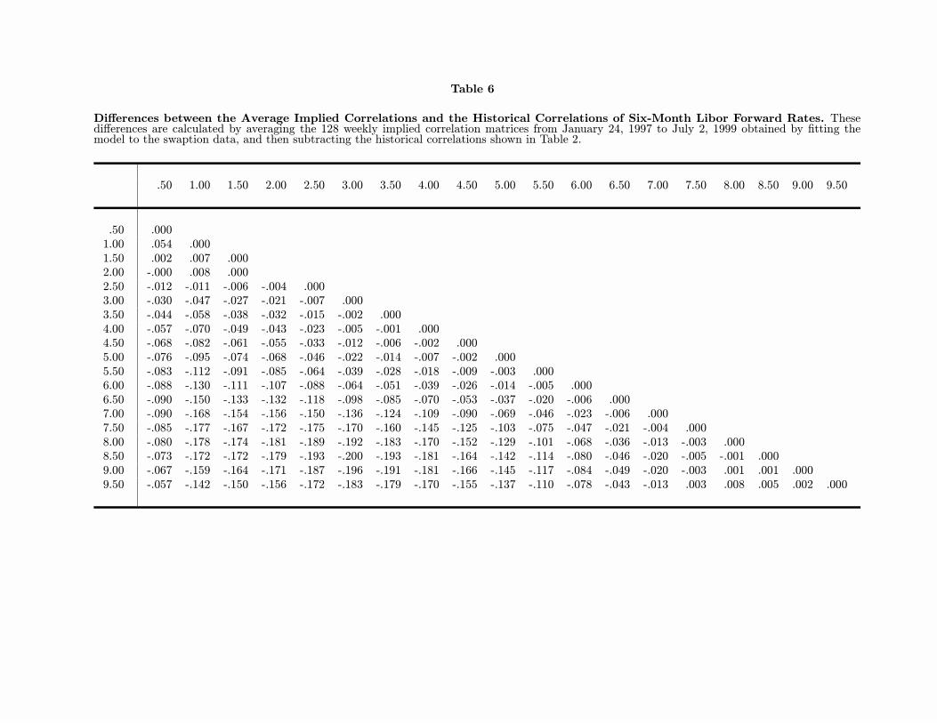
Table 6

Differences between the Average Implied Correlations and the Historical Correlations of Six-Month Libor Forward Rates. Thesedifferences are calculated by averaging the 128 weekly implied correlation matrices from January 24, 1997 to July 2, 1999 obtained by fitting themodel to the swaption data, and then subtracting the historical correlations shown in Table 2.

.50 1.00 1.50 2.00 2.50 3.00 3.50 4.00 4.50 5.00 5.50 6.00 6.50 7.00 7.50 8.00 8.50 9.00 9.50

.50 .0001.00 .054 .0001.50 .002 .007 .0002.00 -.000 .008 .0002.50 -.012 -.011 -.006 -.004 .0003.00 -.030 -.047 -.027 -.021 -.007 .0003.50 -.044 -.058 -.038 -.032 -.015 -.002 .0004.00 -.057 -.070 -.049 -.043 -.023 -.005 -.001 .0004.50 -.068 -.082 -.061 -.055 -.033 -.012 -.006 -.002 .0005.00 -.076 -.095 -.074 -.068 -.046 -.022 -.014 -.007 -.002 .0005.50 -.083 -.112 -.091 -.085 -.064 -.039 -.028 -.018 -.009 -.003 .0006.00 -.088 -.130 -.111 -.107 -.088 -.064 -.051 -.039 -.026 -.014 -.005 .0006.50 -.090 -.150 -.133 -.132 -.118 -.098 -.085 -.070 -.053 -.037 -.020 -.006 .0007.00 -.090 -.168 -.154 -.156 -.150 -.136 -.124 -.109 -.090 -.069 -.046 -.023 -.006 .0007.50 -.085 -.177 -.167 -.172 -.175 -.170 -.160 -.145 -.125 -.103 -.075 -.047 -.021 -.004 .0008.00 -.080 -.178 -.174 -.181 -.189 -.192 -.183 -.170 -.152 -.129 -.101 -.068 -.036 -.013 -.003 .0008.50 -.073 -.172 -.172 -.179 -.193 -.200 -.193 -.181 -.164 -.142 -.114 -.080 -.046 -.020 -.005 -.001 .0009.00 -.067 -.159 -.164 -.171 -.187 -.196 -.191 -.181 -.166 -.145 -.117 -.084 -.049 -.020 -.003 .001 .001 .0009.50 -.057 -.142 -.150 -.156 -.172 -.183 -.179 -.170 -.155 -.137 -.110 -.078 -.043 -.013 .003 .008 .005 .002 .000

Table 7

Standard Deviations of the Implied Correlations of Six-Month Libor Forward Rates. This table reports the standard deviations of theindividual elements of the 128 weekly implied correlation matrices from January 24, 1997 to July 2, 1999 obtained by fitting the model to the swaptiondata, and then subtracting the historical correlations shown in Table 2.

.50 1.00 1.50 2.00 2.50 3.00 3.50 4.00 4.50 5.00 5.50 6.00 6.50 7.00 7.50 8.00 8.50 9.00 9.50

.50 .0001.00 .602 .0001.50 .404 .054 .0002.00 .380 .056 .002 .0002.50 .251 .097 .014 .007 .0003.00 .116 .155 .047 .037 .013 .0003.50 .120 .146 .072 .054 .026 .004 .0004.00 .139 .140 .099 .076 .045 .013 .003 .0004.50 .159 .139 .124 .099 .065 .025 .010 .002 .0005.00 .174 .143 .146 .121 .085 .041 .022 .010 .003 .0005.50 .183 .151 .166 .142 .107 .061 .039 .024 .012 .004 .0006.00 .181 .161 .183 .162 .132 .088 .066 .048 .031 .017 .005 .0006.50 .169 .174 .196 .181 .160 .123 .103 .083 .064 .044 .024 .007 .0007.00 .151 .182 .201 .195 .185 .161 .144 .125 .104 .081 .055 .028 .007 .0007.50 .139 .183 .197 .199 .200 .189 .177 .161 .142 .118 .089 .056 .026 .006 .0008.00 .144 .176 .185 .193 .204 .203 .196 .184 .168 .146 .117 .082 .047 .019 .004 .0008.50 .163 .165 .169 .180 .196 .203 .200 .193 .180 .161 .134 .101 .064 .032 .012 .003 .0009.00 .188 .152 .151 .163 .181 .194 .194 .190 .181 .166 .142 .111 .075 .043 .021 .008 .002 .0009.50 .214 .140 .135 .146 .165 .180 .184 .183 .177 .165 .145 .117 .083 .053 .030 .016 .006 .001 .000

Table 8

Summary Statistics for Percentage Swaption Valuation Errors. The summary statistics reportedare for the differences between the fitted model price and the market price expressed as a percentage of themarket price. The data set consists of 128 weekly observations from January 24, 1997 to July 2, 1999 forthe indicated N into M at-the-money-forward European swaption structures, where N denotes years untiloption expiration and M denotes the tenor or length of the underlying swap in years. The t-statistic forthe mean and the standard deviation reported are adjusted for first-order serial correlation. The overallstatistics are simple averages of the corresponding columns with the exception of the overall minimum,median, and maximum which are computed from all observations.

t-Stat Standard SerialN M Mean Mean Deviation Minimum Median Maximum Correlation

.50 1.00 -2.456 -1.26 1.954 -19.623 -1.032 6.406 .9061.00 1.00 -1.123 -1.45 .775 -12.922 -1.560 5.423 .7272.00 1.00 -2.124 -3.57 .595 -8.583 -2.006 4.383 .7763.00 1.00 -.924 -1.30 .712 -5.146 -1.127 6.726 .8454.00 1.00 .501 .38 1.304 -4.030 -.177 11.406 .9175.00 1.00 4.815 1.95 2.475 -1.209 3.470 24.683 .935

.50 2.00 -1.312 -1.06 1.238 -16.379 -1.033 5.057 .8531.00 2.00 -.538 -1.43 .375 -9.588 -.273 3.654 .5752.00 2.00 -1.542 -3.24 .476 -5.757 -1.577 2.163 .8093.00 2.00 .289 .42 .685 -3.487 -.131 9.523 .8554.00 2.00 1.906 1.35 1.411 -3.041 1.005 14.468 .9165.00 2.00 5.612 2.51 2.239 -.995 4.289 24.027 .924

.50 3.00 -.030 -.01 2.332 -22.139 1.786 8.077 .9071.00 3.00 -1.696 -2.01 .843 -13.825 -1.294 2.517 .8712.00 3.00 -1.920 -7.08 .271 -4.701 -1.907 .794 .7453.00 3.00 .328 .71 .461 -6.406 .112 6.868 .7934.00 3.00 2.033 1.69 1.201 -2.552 1.323 14.843 .8955.00 3.00 5.446 2.51 2.168 -.193 3.976 22.971 .934

.50 4.00 -.547 -.19 2.815 -27.444 1.191 9.925 .8991.00 4.00 -2.523 -1.68 1.503 -16.314 -2.057 3.209 .9232.00 4.00 -2.209 -8.81 .251 -5.382 -2.141 -.034 .7633.00 4.00 .151 .40 .373 -2.371 .014 5.346 .8044.00 4.00 1.775 1.56 1.137 -2.494 1.124 12.965 .9125.00 4.00 5.409 2.64 2.045 -.317 3.839 19.778 .939

.50 5.00 -1.529 -.50 3.079 -32.517 .387 9.693 .8971.00 5.00 -3.013 -2.62 1.149 -18.546 -2.631 6.900 .8142.00 5.00 -2.402 -6.42 .374 -7.244 -2.148 -.087 .8173.00 5.00 -.446 -1.70 .263 -3.433 -.396 3.546 .7434.00 5.00 1.239 1.21 1.026 -1.963 .383 10.447 .9155.00 5.00 5.615 2.79 2.013 -.444 4.609 18.406 .944

.50 7.00 -3.604 -.91 3.941 -40.981 -1.438 9.483 .9091.00 7.00 -5.365 -1.93 2.779 -26.164 -3.978 4.643 .9372.00 7.00 -5.096 -4.36 1.170 -16.876 -4.053 -2.015 .9093.00 7.00 -3.382 -15.35 .220 -7.276 -3.154 -1.265 .669

Overall -.255 -1.38 1.343 -40.981 -.416 24.683 .852

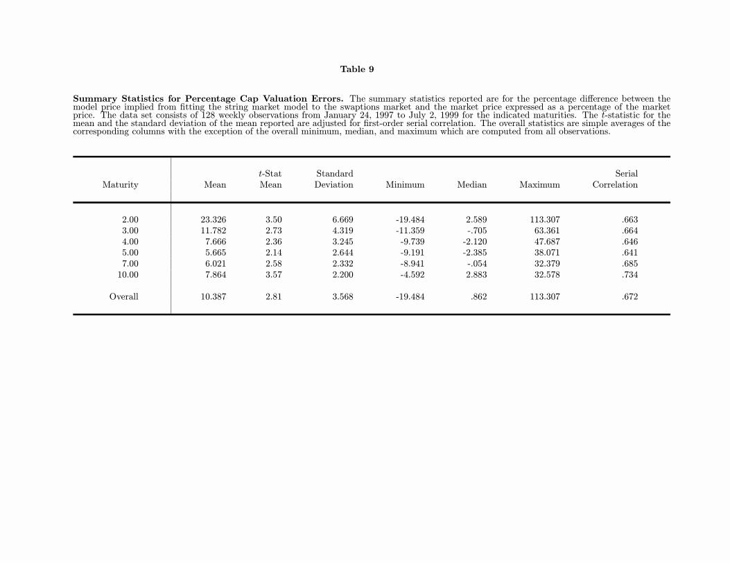
Table 9

Summary Statistics for Percentage Cap Valuation Errors. The summary statistics reported are for the percentage difference between themodel price implied from fitting the string market model to the swaptions market and the market price expressed as a percentage of the marketprice. The data set consists of 128 weekly observations from January 24, 1997 to July 2, 1999 for the indicated maturities. The t-statistic for themean and the standard deviation of the mean reported are adjusted for first-order serial correlation. The overall statistics are simple averages of thecorresponding columns with the exception of the overall minimum, median, and maximum which are computed from all observations.

t-Stat Standard SerialMaturity Mean Mean Deviation Minimum Median Maximum Correlation

2.00 23.326 3.50 6.669 -19.484 2.589 113.307 .6633.00 11.782 2.73 4.319 -11.359 -.705 63.361 .6644.00 7.666 2.36 3.245 -9.739 -2.120 47.687 .6465.00 5.665 2.14 2.644 -9.191 -2.385 38.071 .6417.00 6.021 2.58 2.332 -8.941 -.054 32.379 .68510.00 7.864 3.57 2.200 -4.592 2.883 32.578 .734

Overall 10.387 2.81 3.568 -19.484 .862 113.307 .672

Table 10

Summary Statistics for Percentage Cap Valuation Errors from a One-Factor Model. The summary statistics reported are for thepercentage difference between the model price implied from the one-factor version of the string market model in which the correlations between allforward rates are assumed to equal one and the market price expressed as a percentage of the market price. The data set consists of 128 weeklyobservations from January 24, 1997 to July 2, 1999 for the indicated maturities. The t-statistic for the mean and the standard deviation of the meanreported are adjusted for first-order serial correlation. The overall statistics are simple averages of the corresponding columns with the exception ofthe overall minimum, median, and maximum which are computed from all observations, and number positive which is the total over all observations.

t-Stat Standard Number SerialMaturity Mean Mean Deviation Minimum Median Maximum Positive Correlation

2.00 -25.286 -7.76 3.259 -62.054 -23.639 -9.359 0 .8853.00 -23.400 -14.12 1.657 -46.757 -22.431 -8.721 0 .8274.00 -20.288 -24.39 .832 -33.633 -19.423 -13.697 0 .7175.00 -17.500 -31.59 .554 -26.244 -16.969 -6.238 0 .6317.00 -11.320 -27.77 .408 -20.658 -11.132 3.732 1 .52910.00 -5.884 -8.63 .682 -13.457 -5.954 12.071 7 .716

Overall -17.279 -19.04 1.232 -62.054 -17.371 12.071 8 .718

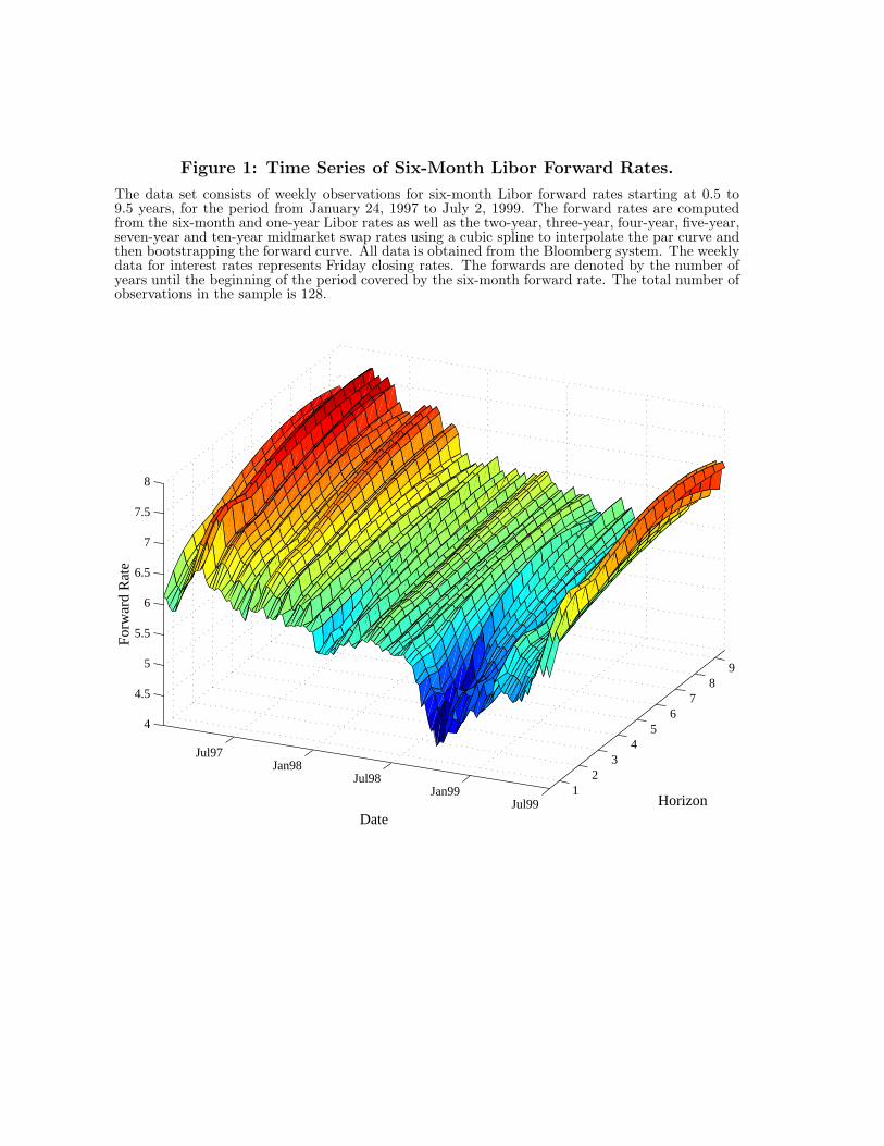
Figure 1: Time Series of Six-Month Libor Forward Rates.

The data set consists of weekly observations for six-month Libor forward rates starting at 0.5 to9.5 years, for the period from January 24, 1997 to July 2, 1999. The forward rates are computedfrom the six-month and one-year Libor rates as well as the two-year, three-year, four-year, five-year,seven-year and ten-year midmarket swap rates using a cubic spline to interpolate the par curve andthen bootstrapping the forward curve. All data is obtained from the Bloomberg system. The weeklydata for interest rates represents Friday closing rates. The forwards are denoted by the number ofyears until the beginning of the period covered by the six-month forward rate. The total number ofobservations in the sample is 128.

12

34

56

78

9

Jul99Jan99

Jul98Jan98

Jul97

4

4.5

5

5.5

6

6.5

7

7.5

8

HorizonDate

For

war

d R

ate

Figure 2: Time Series of Swaption Volatilities.

The data set consists of 128 weekly observations from January 24, 1997 to July 2, 1999 of midmarketimplied Black-model volatilities for the indicated N into M at-the-money-forward European swap-tion structure, where N denotes years until option expiration (time to maturity) and M denotes thelength of the underlying swap in years (the tenor). The sub-plots show, for each tenor, the impliedvolatilities of options with different times to maturity.

0.51

23

45

Jul99Jan99Jul98Jan98Jul97

10

15

20

25

30

Time to Maturity

One−Year Tenor

Date

Swap

tion

Vol

atili

ty

0.51

23

45

Jul99Jan99Jul98Jan98Jul97

10

15

20

25

30

Time to Maturity

Two−Year Tenor

Date

Swap

tion

Vol

atili

ty

0.51

23

45

Jul99Jan99Jul98Jan98Jul97

10

15

20

25

30

Time to Maturity

Three−Year Tenor

Date

Swap

tion

Vol

atili

ty

0.51

23

45

Jul99Jan99Jul98Jan98Jul97

10

15

20

25

30

Time to Maturity

Four−Year Tenor

Date

Swap

tion

Vol

atili

ty

0.51

23

45

Jul99Jan99Jul98Jan98Jul97

10

15

20

25

30

Time to Maturity

Five−Year Tenor

Date

Swap

tion

Vol

atili

ty

0.5

1

2

3

Jul99Jan99Jul98Jan98Jul97

10

15

20

25

30

Time to Maturity

Seven−Year Tenor

Date

Swap

tion

Vol

atili

ty

Figure 3: Examples of Swaption Volatility Surfaces.

This figure plots the quoted volatilities of swaptions on four different dates of the sample. Eachfigure shows quotes for swaptions with maturities between 0.5 and 5 years on underlying swaps withhorizons at the maturity of the options between 1 and 7 years. Note that we do not use the 4 into7 and the 5 into 7 swaptions in the empirical study since they are less liquid.

0.5 1 2 3 4 5 12

34

5715

16

17

18

19

Tenor

Jan 24,1997

Time to Maturity

Swap

tion

Vol

atili

ty

0.5 1 2 3 4 5 12

34

5713

14

15

16

Tenor

Nov 28, 1997

Time to Maturity

Swap

tion

Vol

atili

ty

0.5 1 2 3 4 5 12

34

5710

15

20

25

30

Tenor

Oct 9, 1998

Time to Maturity

Swap

tion

Vol

atili

ty

0.5 1 2 3 4 5 12

34

5714

15

16

17

Tenor

July 2, 1999

Time to Maturity

Swap

tion

Vol

atili

ty

Figure 4: Time Series of Cap Volatilities.

The data set consists of 128 weekly observations from January 24, 1997 to July 2, 1999 of midmarketimplied Black-model volatilities for the indicated cap maturities.

2

3

4

5

7

10

Jul99Jan99

Jul98Jan98

Jul97

10

12

14

16

18

20

22

24

26

28

MaturityDate

Cap

Vol

atili

ty

Figure 5: Eigenvector Weights.

The four subplots show the weights of the first four eigenvectors of the historical correlation matrix.The correlation matrix is based on weekly changes in the logarithm of individual six-month Liborforward rates for the ex ante period from January 17, 1992 to January 17, 1997. The forward ratesare computed from the six-month and one-year Libor rates as well as the two-year, three-year, four-year, five-year, seven-year and ten-year midmarket swap rates using a cubic spline to interpolate thepar curve and then bootstrapping the forward curve. The weekly data for interest rates representsFriday closing rates. The horizons of the six-month forward rates used to compute the correlationmatrix range from 0.50 years to 9.50 years forward, giving a total of 19 time series of forward rates.The total number of observations is 262.

1 3 5 7 9 11 13 15 17 19−0.5

−0.25

0

0.25

Horizon

Wei

ghts

First Eigenvector

1 3 5 7 9 11 13 15 17 19−0.5

−0.25

0

0.25

Horizon

Wei

ghts

Second Eigenvector

1 3 5 7 9 11 13 15 17 19−0.5

−0.25

0

0.25

Horizon

Wei

ghts

Third Eigenvector

1 3 5 7 9 11 13 15 17 19−0.5

−0.25

0

0.25

Horizon

Wei

ghts

Fourth Eigenvector

Figure 6: Time Series of Eigenvalues.

The four subplots show the eigenvalues computed from the 128 weekly implied correlation matricesfrom January 24, 1997 to July 2, 1999 obtained by fitting the model to the swaption data, keepingfixed the eigenvectors of the historical correlation matrix.

Jan97 Jul97 Jan98 Jul98 Jan990

0.1

0.2

0.3

0.4

0.5

Date

Eig

enva

lue

First Eigenvalue

Jan97 Jul97 Jan98 Jul98 Jan990

0.1

0.2

0.3

0.4

0.5

Date

Eig

enva

lue

Second Eigenvalue

Jan97 Jul97 Jan98 Jul98 Jan990

0.1

0.2

0.3

0.4

0.5

Date

Eig

enva

lue

Third Eigenvalue

Jan97 Jul97 Jan98 Jul98 Jan990

0.1

0.2

0.3

0.4

0.5

Date

Eig

enva

lue

Fourth Eigenvalue

Figure 7: Time Series of Swaptions RMSE of Four-Factor String MarketModel.

The graph shows the RMSE of the the differences between the fitted model swaptions prices and themarket prices expressed as a percentage of the market prices. The data set consists of 128 weeklyobservations from January 24, 1997 to July 2, 1999 for 34 at-the-money-forward European swaptionstructures.

Jan97 Jun97 Oct97 Mar98 Aug98 Dec98 May990

2

4

6

8

10

12

14

16

18

Date

Perc

ent P

rici

ng E

rror