the relationship between the low salinity zone...
TRANSCRIPT
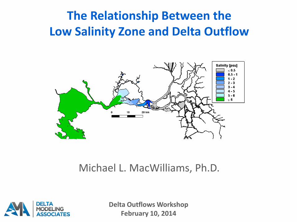
Michael L. MacWilliams, Ph.D.
The Relationship Between the Low Salinity Zone and Delta Outflow
Delta Outflows Workshop
February 10, 2014
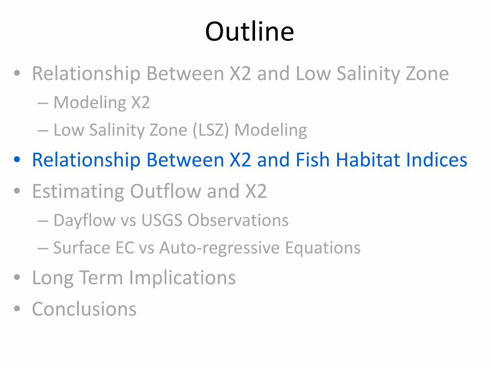
Outline • Relationship Between X2 and Low Salinity Zone
– Modeling X2 – Low Salinity Zone (LSZ) Modeling
• Relationship Between X2 and Fish Habitat Indices • Estimating Outflow and X2
– Dayflow vs USGS Observations – Surface EC vs Auto-regressive Equations
• Long Term Implications • Conclusions
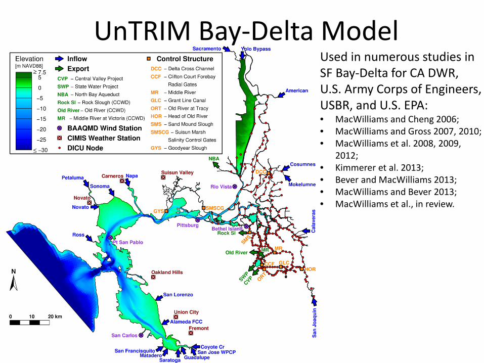
UnTRIM Bay-Delta Model Used in numerous studies in SF Bay-Delta for CA DWR, U.S. Army Corps of Engineers, USBR, and U.S. EPA: • MacWilliams and Cheng 2006; • MacWilliams and Gross 2007, 2010; • MacWilliams et al. 2008, 2009,
2012; • Kimmerer et al. 2013; • Bever and MacWilliams 2013; • MacWilliams and Bever 2013; • MacWilliams et al., in review.
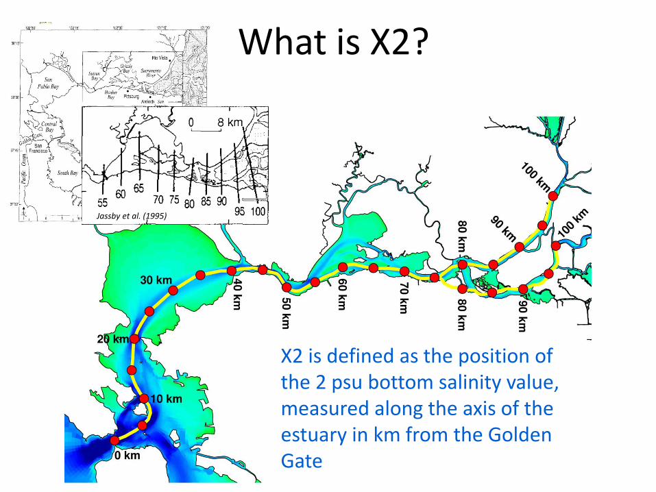
What is X2?
X2 is defined as the position of the 2 psu bottom salinity value, measured along the axis of the estuary in km from the Golden Gate
Jassby et al. (1995)
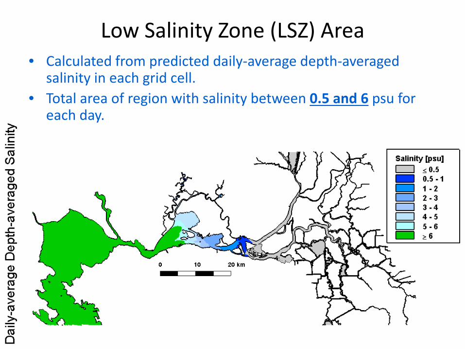
Low Salinity Zone (LSZ) Area • Calculated from predicted daily-average depth-averaged
salinity in each grid cell. • Total area of region with salinity between 0.5 and 6 psu for
each day.
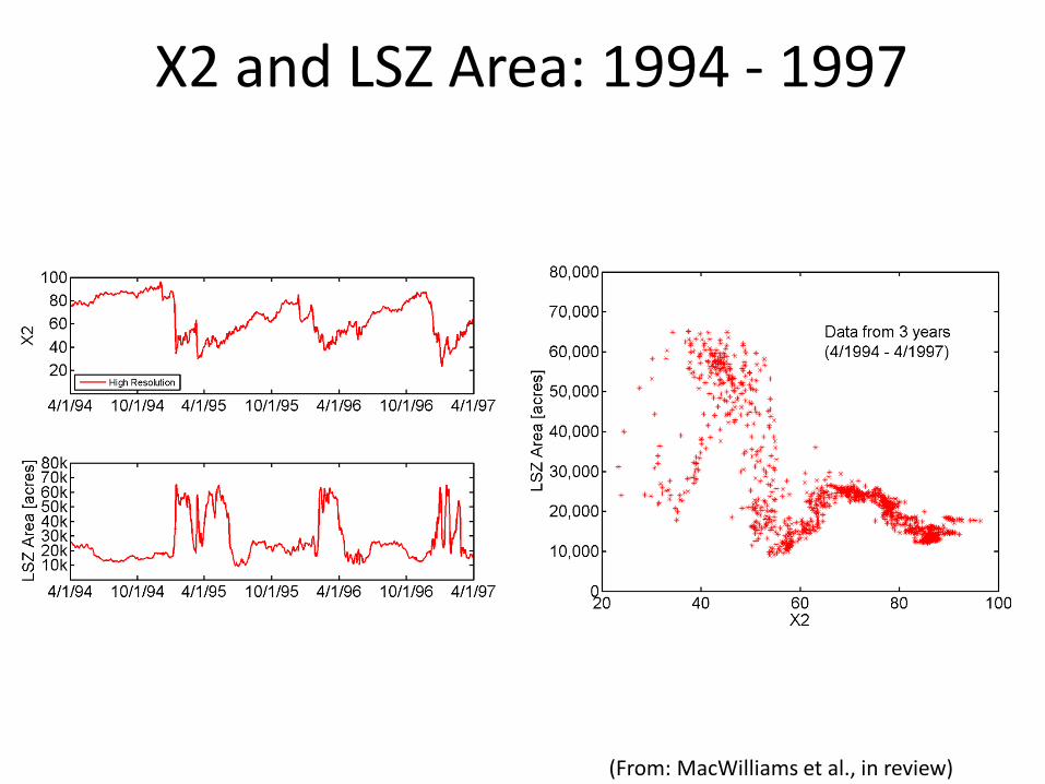
X2 and LSZ Area: 1994 - 1997
(From: MacWilliams et al., in review)
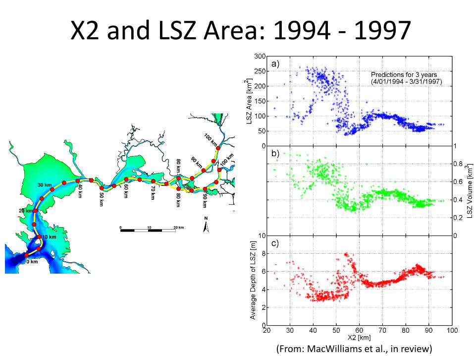
X2 and LSZ Area: 1994 - 1997
(From: MacWilliams et al., in review)
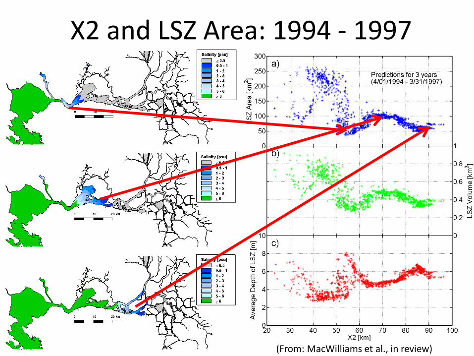
X2 and LSZ Area: 1994 - 1997
(From: MacWilliams et al., in review)
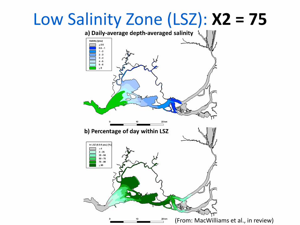
Low Salinity Zone (LSZ): X2 = 75
(From: MacWilliams et al., in review)
Outline • Relationship Between X2 and Low Salinity Zone
– Modeling X2 – Low Salinity Zone (LSZ) Modeling
• Relationship Between X2 and Fish Habitat Indices • Estimating Outflow and X2
– Dayflow vs USGS Observations – Surface EC vs Auto-regressive Equations
• Long Term Implications • Conclusions
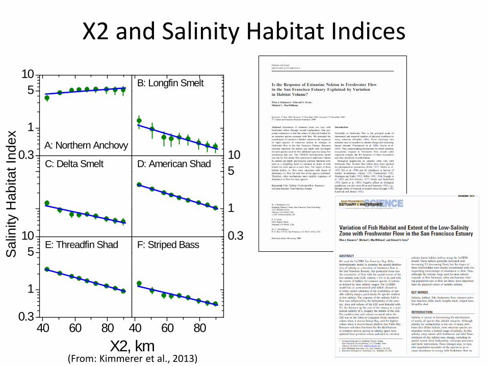
X2 and Salinity Habitat Indices
0.3
1
510
0.3
1
510
40 60 800.3
1
510
40 60 80
A: Northern Anchovy
B: Longfin Smelt
C: Delta Smelt
Habi
tat I
ndex D: American Shad
X2, km
E: Threadfin Shad F: Striped Bass
(From: Kimmerer et al., 2013)
Salin
ity H
abita
t Ind
ex

Outline • Relationship Between X2 and Low Salinity Zone
– Modeling X2 – Low Salinity Zone (LSZ) Modeling
• Relationship Between X2 and Fish Habitat Indices • Estimating Outflow and X2
– Dayflow vs USGS Observations – Surface EC vs Auto-regressive Equations
• Long Term Implications • Conclusions
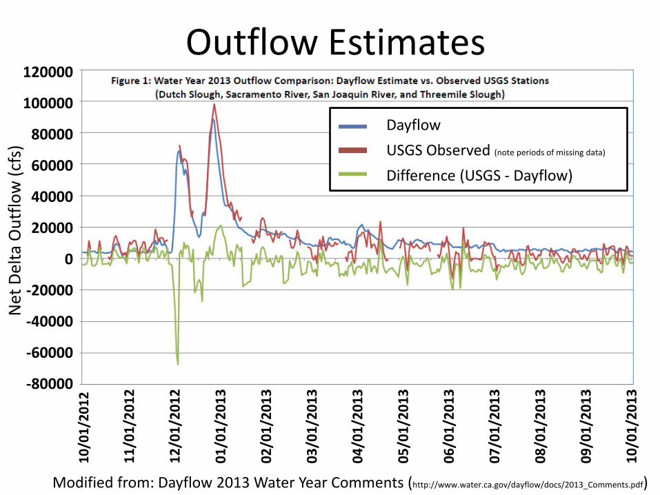
Modified from: Dayflow 2013 Water Year Comments (http://www.water.ca.gov/dayflow/docs/2013_Comments.pdf)
120000
100000
80000
60000
40000
20000
0
-20000
-40000
-60000
-80000
Net
Del
ta O
utflo
w (c
fs)
Dayflow USGS Observed (note periods of missing data)
Difference (USGS - Dayflow)
Outflow Estimates 10
/01/
2012
11/0
1/20
12
12/0
1/20
12
01/0
1/20
13
02/0
1/20
13
03/0
1/20
13
04/0
1/20
13
05/0
1/20
13
06/0
1/20
13
07/0
1/20
13
08/0
1/20
13
09/0
1/20
13
10/0
1/20
13
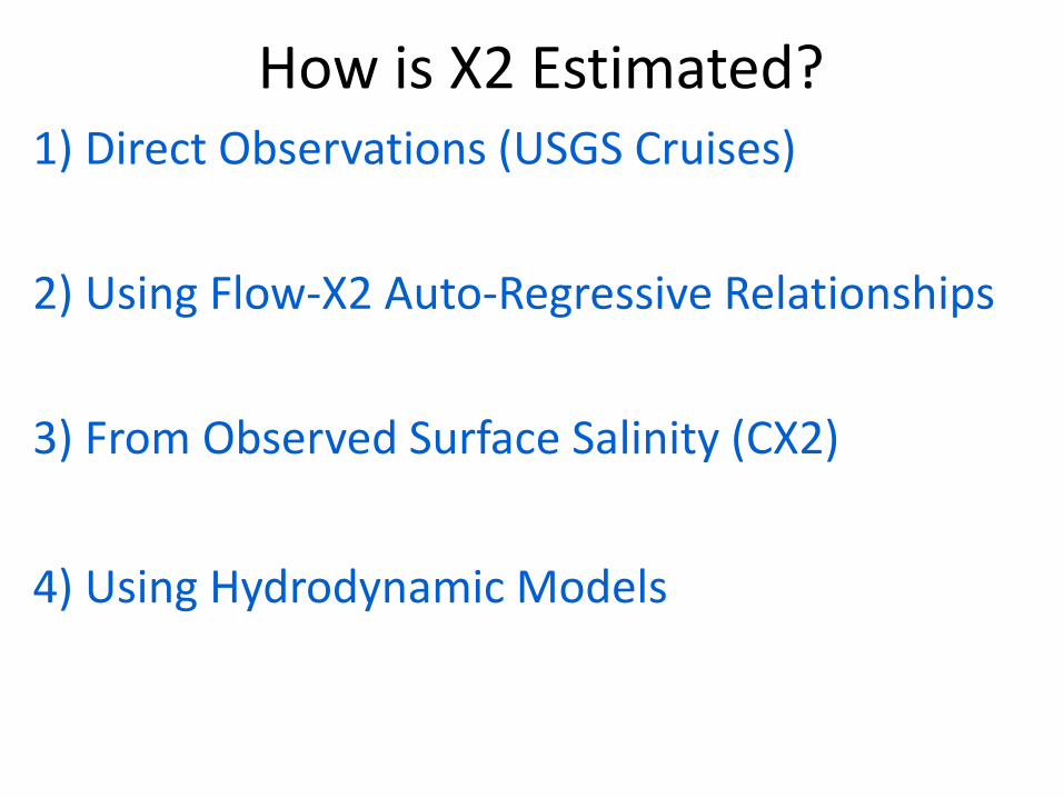
1) Direct Observations (USGS Cruises) 2) Using Flow-X2 Auto-Regressive Relationships 3) From Observed Surface Salinity (CX2) 4) Using Hydrodynamic Models
How is X2 Estimated?
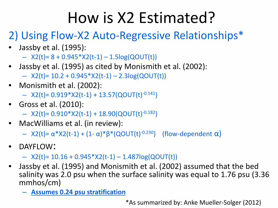
2) Using Flow-X2 Auto-Regressive Relationships* • Jassby et al. (1995):
– X2(t)= 8 + 0.945*X2(t-1) – 1.5log(QOUT(t)) • Jassby et al. (1995) as cited by Monismith et al. (2002):
– X2(t)= 10.2 + 0.945*X2(t-1) – 2.3log(QOUT(t)) • Monismith et al. (2002):
– X2(t)= 0.919*X2(t-1) + 13.57(QOUT(t)-0.141) • Gross et al. (2010):
– X2(t)= 0.910*X2(t-1) + 18.90(QOUT(t)-0.182) • MacWilliams et al. (in review):
– X2(t)= α*X2(t-1) + (1- α)*β*(QOUT(t)-0.230) (flow-dependent α) • DAYFLOW:
– X2(t)= 10.16 + 0.945*X2(t-1) – 1.487log(QOUT(t)) • Jassby et al. (1995) and Monismith et al. (2002) assumed that the bed
salinity was 2.0 psu when the surface salinity was equal to 1.76 psu (3.36 mmhos/cm) – Assumes 0.24 psu stratification
How is X2 Estimated?
*As summarized by: Anke Mueller-Solger (2012)
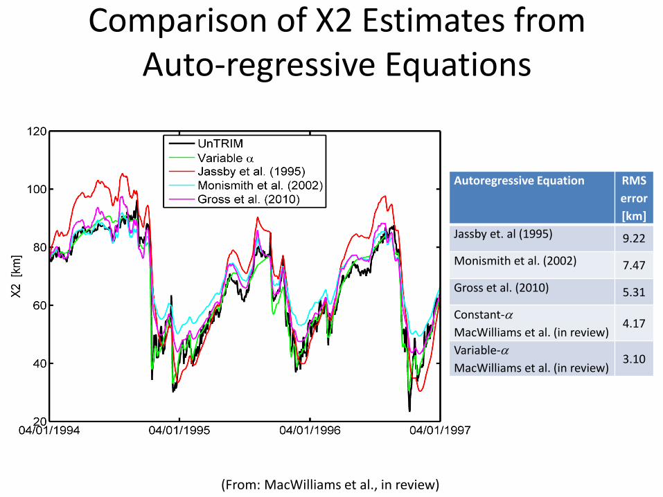
Comparison of X2 Estimates from Auto-regressive Equations
(From: MacWilliams et al., in review)
Autoregressive Equation RMS error [km]
Jassby et. al (1995) 9.22
Monismith et al. (2002) 7.47
Gross et al. (2010) 5.31
Constant-α MacWilliams et al. (in review)
4.17
Variable-α MacWilliams et al. (in review)
3.10
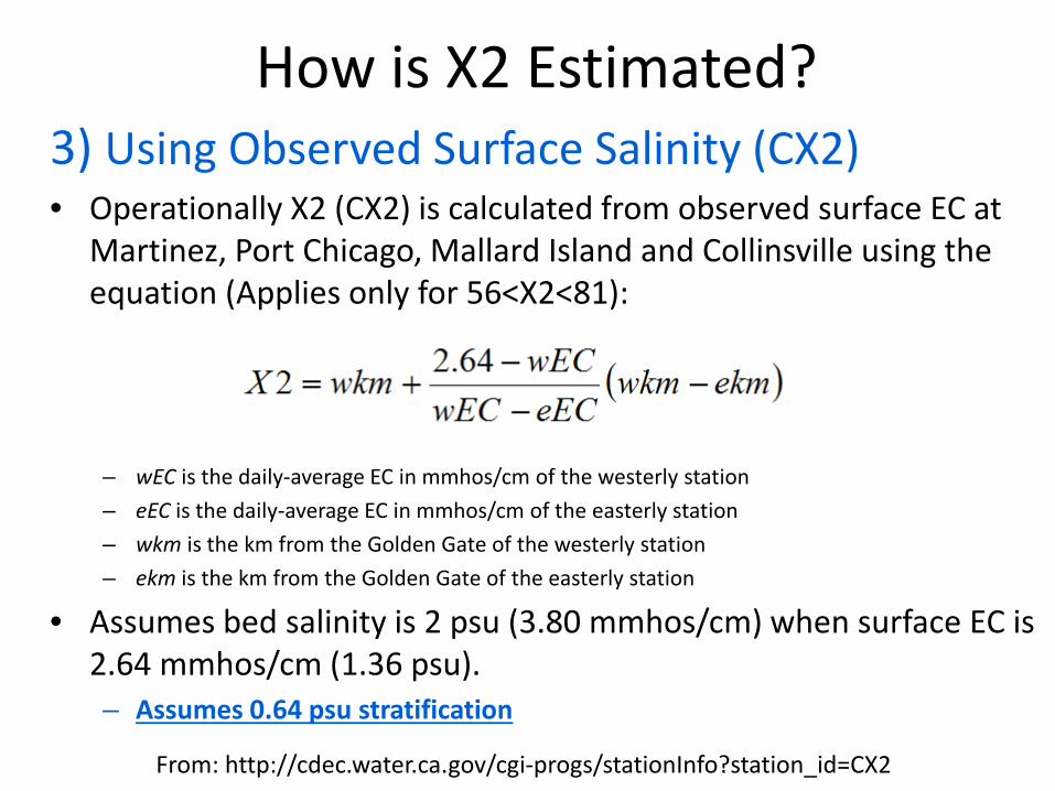
3) Using Observed Surface Salinity (CX2) • Operationally X2 (CX2) is calculated from observed surface EC at
Martinez, Port Chicago, Mallard Island and Collinsville using the equation (Applies only for 56<X2<81): – wEC is the daily-average EC in mmhos/cm of the westerly station – eEC is the daily-average EC in mmhos/cm of the easterly station – wkm is the km from the Golden Gate of the westerly station – ekm is the km from the Golden Gate of the easterly station
• Assumes bed salinity is 2 psu (3.80 mmhos/cm) when surface EC is 2.64 mmhos/cm (1.36 psu). – Assumes 0.64 psu stratification
How is X2 Estimated?
From: http://cdec.water.ca.gov/cgi-progs/stationInfo?station_id=CX2

Surface Salinity vs. Bed Salinity Evaluation of CX2:
Assumes 0.64 psu stratification
Assumption of 0.64 psu stratification (2.64 mmhos/cm surface EC) tends to over predict X2 relative to X2 calculated from PREDICTED bed salinity
Assumption of 0.24 psu stratification (3.37 mmhos/cm surface EC) tends to under predict X2 relative to X2 calculated from OBSERVED bed salinity
Evaluation of Jassby et al. (1995): Assumes 0.24 psu stratification
Outline • Relationship Between X2 and Low Salinity Zone
– Modeling X2 – Low Salinity Zone (LSZ) Modeling
• Relationship Between X2 and Fish Habitat Indices • Estimating Outflow and X2
– Dayflow vs USGS Observations – Surface EC vs Auto-regressive Equations
• Long Term Implications • Conclusions
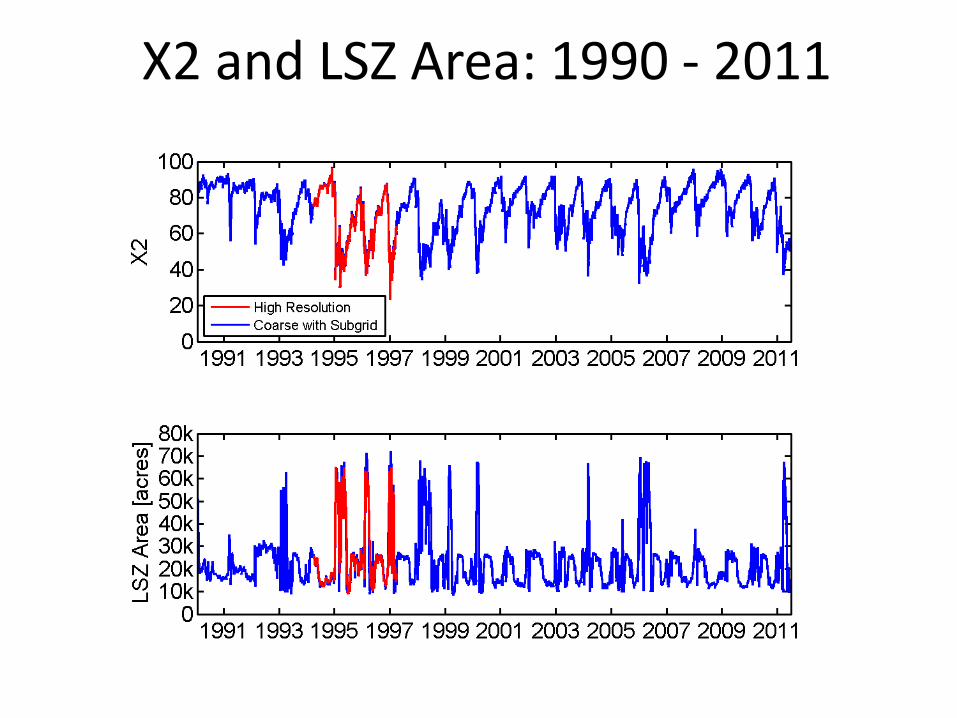
X2 and LSZ Area: 1990 - 2011

LSZ Area vs. X2
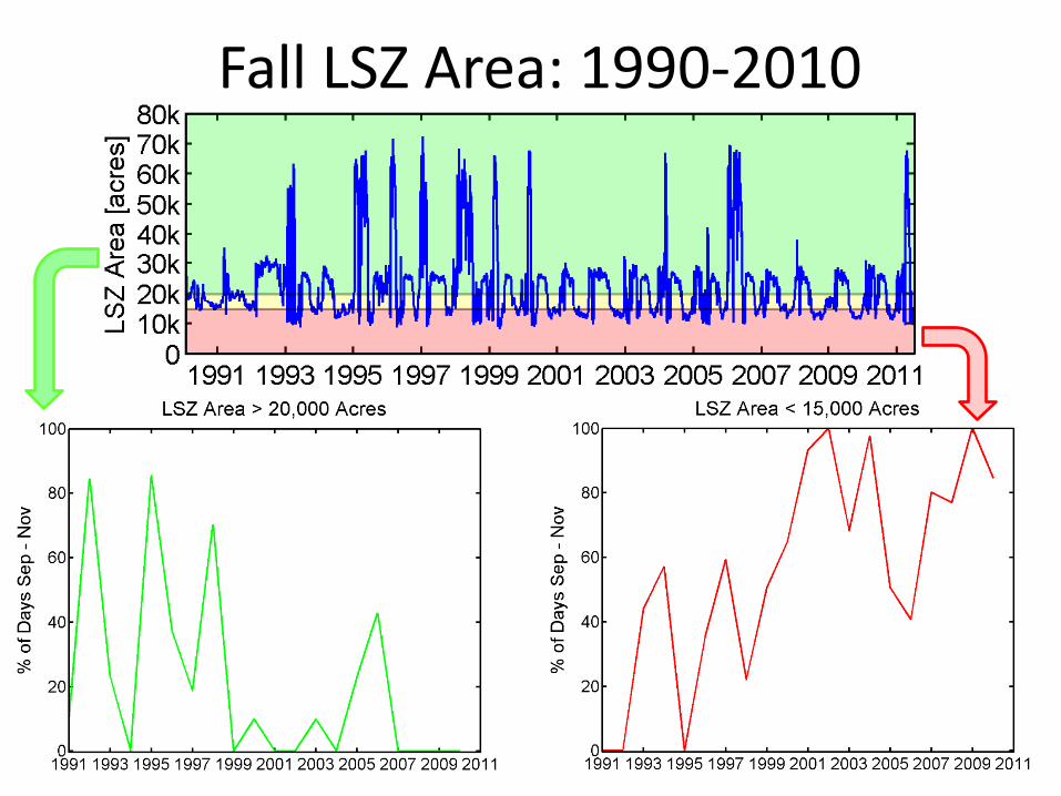
Fall LSZ Area: 1990-2010
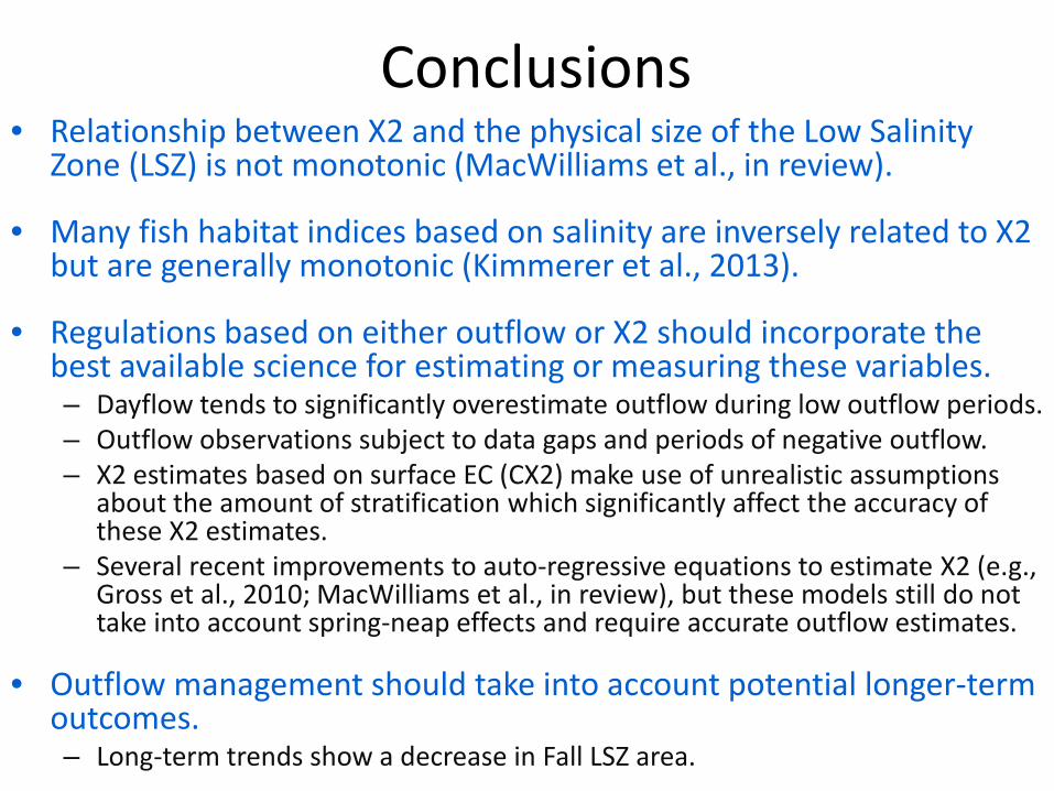
Conclusions • Relationship between X2 and the physical size of the Low Salinity
Zone (LSZ) is not monotonic (MacWilliams et al., in review).
• Many fish habitat indices based on salinity are inversely related to X2 but are generally monotonic (Kimmerer et al., 2013).
• Regulations based on either outflow or X2 should incorporate the best available science for estimating or measuring these variables. – Dayflow tends to significantly overestimate outflow during low outflow periods. – Outflow observations subject to data gaps and periods of negative outflow. – X2 estimates based on surface EC (CX2) make use of unrealistic assumptions
about the amount of stratification which significantly affect the accuracy of these X2 estimates.
– Several recent improvements to auto-regressive equations to estimate X2 (e.g., Gross et al., 2010; MacWilliams et al., in review), but these models still do not take into account spring-neap effects and require accurate outflow estimates.
• Outflow management should take into account potential longer-term outcomes. – Long-term trends show a decrease in Fall LSZ area.
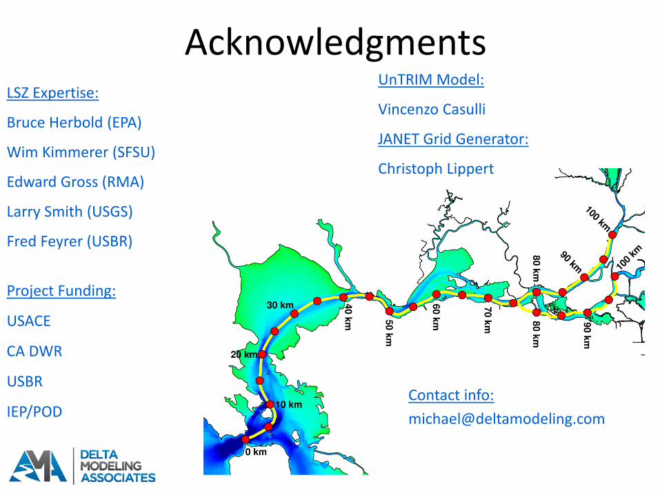
Acknowledgments UnTRIM Model:
Vincenzo Casulli
JANET Grid Generator:
Christoph Lippert
LSZ Expertise:
Bruce Herbold (EPA)
Wim Kimmerer (SFSU)
Edward Gross (RMA)
Larry Smith (USGS)
Fred Feyrer (USBR)
Project Funding:
USACE
CA DWR
USBR
IEP/POD Contact info: [email protected]