the relationship between the bending amplitude and …
TRANSCRIPT

THE RELATIONSHIP BETWEEN THE BENDING AMPLITUDE AND
BENDING STRESS/STRAIN AT THE MOUTH OF A SO-CALLED SQUARE-
FACED CLAMP FOR DIFFERENT CONDUCTOR SIZES AND DIFFERENT
TENSILE LOADS: EXPERIMENTAL APPROACH
by
Yatshamba Daniel Kubelwa
(Student Number: 211559874)
Submitted in fulfilment of the academic requirements for the degree of Master of Science
in Mechanical Engineering
School of Engineering,
Discipline of Mechanical Engineering,
Supervisor: Dr Richard Loubser
Co-supervisor: Dr Konstantin O. Papailiou
University of KwaZulu-Natal Durban
February 2013
As the candidate’s supervisor I have/have not approved this thesis/dissertation for
submission.
Signed: _____________ Name Date: 16 February 2013
Dr Richard Loubser (Supervisor)

“For my father Leonard Kubelwa Musaya and in
memories of my lovely mother Audrey Kakenge
Bushindi”

The University of KwaZulu-Natal
i
Abstract
In this research, realistic models were developed using experimental approach and statistical or
deterministic analysis in the relationship between bending amplitudes and bending stress (strain)
of the overhead line conductor. This was rigidity clamped and subjected to Aeolian vibration
(1Hz-150 Hz). The experiments were performed at the Vibration Research and Testing Centre
(VRTC) laboratory of the University of KwaZulu-Natal. A shaker connected to the conductor
was used to simulate the Aeolian vibration and transducers (accelerometers, thermocouples and
strain-gauges) to control the shaker and collect data. For almost half a century, in transmission
lines, bending stress which is a key factor in determining the life expectancy prediction of
overhead conductor is assessed by using an idealized model the so-called Poffenberger-Swart
formula based on cantilever beam theory and many assumptions [2].
Four overhead line ACSR (Aluminum conductor steel-reinforced) conductors i.e. Rabbit (6 Al.
/1St.), Pelican (18 Al. /1St.), Tern (45 Al./7St.) and Bersfort(48 Al./7St.) were investigated at
three different ranges of tensile load i.e. 20 %, 25%, and 30% Ultimate Tensile Strength (UTS).
Bending amplitudes (0.0 1mm -1.2mm) and bending stresses measurements were collected and
plotted as bending stress σb versus bending amplitude Yb, curve-fitting with polynomial function
of the third order in terms of four parameters (where curve fitting coefficients B0, B1, B2, and B3)
provided excellent simulations (predictions) of the experimental data for the conductors.
However, it was found that the accuracy of the fit is not improved by the inclusion of higher order
terms. Therefore, only four-parameters (for all cases high order than 3 are ambiguous, in spite of
the Regression parameter or predictor were R2 ≥ 0.998 but Standard errors were large). It was
noticed that the precedent model is the simplest polynomial to be employed for the
characterization of all conductors investigated (for all three wires). Other ways to obtain the best
curve fittings were explored and discussed such as power model. The experimental results were
compared to the Poffenberger-Swart model. In all cases, it was observed that the deviation from
the results to the above model is significant for small bending amplitudes and is small for high
bending amplitudes and good correlations were observed when associated this with the bending
stiffness model developed by Papailiou [17].

The University of KwaZulu-Natal
ii
Preface
The experimental work described in this dissertation was carried out at The Vibration
Research and Testing Centre (VRTC) in the School of Engineering, University of
KwaZulu-Natal, Durban, from April 2011 to January 2013, under the supervision of
Dr Richard Loubser and Dr Konstantin O. Papailiou.
These studies represent original work by the author and have not otherwise been
submitted in any form for any degree or diploma to any tertiary institution. Where
use has been made of the work of others it is duly acknowledged in the text.
YD. Kubelwa

The University of KwaZulu-Natal
iii
DECLARATION 1 - PLAGIARISM
I, Yatshamba Daniel Kubelwa declare that
1. The research reported in this thesis, except where otherwise indicated, is my
original research.
2. This thesis has not been submitted for any degree or examination at any other
university.
3. This thesis does not contain other persons’ data, pictures, graphs or other
information, unless specifically acknowledged as being sourced from other
persons.
4. This thesis does not contain other persons' writing, unless specifically
acknowledged as being sourced from other researchers. Where other written
sources have been quoted, then:
a. Their words have been re-written but the general information attributed
to them has been referenced
b. Where their exact words have been used, then their writing has been
placed in italics and inside quotation marks, and referenced.
5. This thesis does not contain text, graphics or tables copied and pasted from
the Internet, unless specifically acknowledged, and the source being detailed
in the thesis and in the References sections.
Signed: …………………………………………………………

The University of KwaZulu-Natal
iv
DECLARATION 2 - PUBLICATIONS
DETAILS OF CONTRIBUTION TO PUBLICATIONS that form part and/or include research
presented in this thesis (include publications in preparation, submitted, in press and published
and give details of the contributions of each author to the experimental work and writing of
each publication)
Publication 1
YD. Kubelwa, KO Papailiou, R. Loubser and P. Moodley, How Well Does the Poffenberger-
Swart Formula Apply to Homogeneous Compact Overhead Line Conductors? Experimental
Analysis on the Aero-Z® 455-2z Conductor, 18th WCNDT, ISBN: 978-0-620-52872-6,
Durban, 4000, April 2012.
Publication 2
YD. Kubelwa, KO. Papailiou, R. Loubser and P. Moodley, Assessment of Bending
Amplitude-Bending Stress Relation of Single Steel Core Overhead Line ACSR Conductor:
Statistical or Determinist Approach, Cigre Auckland 2013 (in preparation)
Publication 3
YD. Kubelwa, R. Loubser, KO. Papailiou, and P Moodley, Probabilistic modeling of
Bending Stress for Single overhead transmission line rigidly clamped. (In preparation)
Signed: …………...……………………………………………..

The University of KwaZulu-Natal
v
Acknowledgements
May the Almighty God be glorified in Jesus-Christ’s name my King and Saviour!
I gratefully acknowledge my supervisor Dr Richard Loubser, The Vibration Research and
Testing Centre (VRTC) grant holder. I am grateful to my co-supervisor, my mentor and the
promoter of this research Dr Konstantin O. Papailiou, Cigre B2 (Overhead Lines) chairman.
Big thanks to Mr Pravesh Moodley for the technical assistance and his passion for the VRTC
lab. During this thesis, I also received advice from Mr Umberto Cosmai, Mr Charles B.
Rawlins, Dr David G. Havard, Professor Glen Bright, Dr Frederic Levesque (University of
Laval), Dr Freddie Inambao, Mr Bharat Haridass, Mr Joseph Kapuku, Mr Remy Badibanga
and Mr Evans Ojo. I am grateful to Professor Alex Arujo and Professor Aida A. Fadel, the
Lab move and their team at the University of Brasilia where I learnt a lot during my training.
I am grateful to the VRTC, Eskom, Pfisterer and Aberdare Cable for their sponsorship and
donations. Special thanks to Mr Logan Pillay, Eskom Academy of Learning, Mr Henni
Scholtz, Aberdare Cables and Mr Thabani Nene, Pfisterer (South Africa) “the power
connection”.
Many thanks to my Cigre family and especially to the B2 study committee for the
extraordinary works.
The unconditional support of my lovely family “les Kubelwas” is gratefully acknowledged.
YD. Kubelwa

The University of KwaZulu-Natal
vi
Table of Contents
Abstract…………………………………………………………………………………..i
Preface.... ........................................................................................................................... ii
DECLARATION 1 - PLAGIARISM .......................................................................... iii
DECLARATION 2 - PUBLICATIONS ...................................................................... iv
Acknowledgements ......................................................................................................... ..v
Abbreviations………………………………………………………………………….viii
List of Figures .............................................................................................................. viiix
List of Tables ................................................................................................................. xiii
List of Symbols .............................................................................................................. xiv
CHAPTER 1
INTRODUCTION ............................................................................................................ 1
1.1 Problem definition ................................................................................................... 1
1.2 Background .............................................................................................................. 2
1.3 Research Question ................................................................................................... 3
1.4 Project Aims and Objectives.................................................................................... 4
1.5 Applications of the outcomes of the study .............................................................. 4
1.6 Assumptions of this experimental approach ............................................................ 5
1.7 Research Overview .................................................................................................. 6
CHAPTER 2
LITERATURE REVIEW ................................................................................................ 7
2.1 Introduction .............................................................................................................. 7
2.2 Bending amplitude method . .................................................................................... 9
2.3 Conductor stiffness ................................................................................................ 17
2.4 Previous laboratory work ....................................................................................... 21
2.5 Use of statistical tools and techniques ................................................................... 25
2.6 Summary ................................................................................................................ 27
CHAPTER 3
EXPERIMENTAL EQUIPMENT AND PROGRAMME ......................................... 29
3.1. Background ............................................................................................................ 29
3.2 Laboratory configuration and equipment .............................................................. 29
3.3 Materials ................................................................................................................ 31
3.4 Experimental Methodology ................................................................................... 34

The University of KwaZulu-Natal
vii
3.5 Experimental Analysis ........................................................................................... 43
3.6 Summary ................................................................................................................ 48
CHAPTER 4
EXPERIMENTAL RESULTS ...................................................................................... 49
4.1. Background ............................................................................................................ 49
4.2. ACSR Rabbit conductor ........................................................................................ 50
4.3. ACSR Pelican conductor ....................................................................................... 51
4.4. ACSR Tern Conductor........................................................................................... 52
4.5. ACSR Bersfort ....................................................................................................... 53
4.6. Comparison to previous experimental work .......................................................... 55
4.7. Comparison between experimental, Poffenberger-Swart and Papailiou Model .... 56
4.8. Summary ................................................................................................................ 60
CHAPTER 5
STATISTICAL EVALUATION OF TEST RESULTS .............................................. 61
5.1. Background ............................................................................................................ 61
5.2. Prediction models of bending stress ...................................................................... 61
5.3. Stress function parameters ..................................................................................... 62
5.4. Effect of tension level in stress distribution (size effect) ....................................... 74
5.5. Summary ................................................................................................................ 74
CHAPTER 6
CONCLUSION AND FUTURE WORK ..................................................................... 76
List of references ............................................................................................................ 78
Appendices ...................................................................................................................... 82
A Characteristics of different types of conductor motion
B ACSR conductors used in South Africa
C Methods used to determine the resonance frequency
D Results on Static strain measurement
E Results on dynamic stress
F Evaluation Lifetime and Vibration severity (CIGRE)
G Copy of Conference Publication

The University of KwaZulu-Natal
viii
Abbreviations
ACSR Aluminium conductor steel reinforced
ALCOA Aluminium Company of America
ANOVA Analyse of Variance
ASD Allowable Stress Design
CIGRE International Council on Large electric Systems
DAQ Data Acquisition
DOF Degree-of-freedom
EDS Every Day Stress
EHV Extra High Voltage
EPRI Electrical Power Research Institute
ESKOM Electricity Supply Commission (South Africa)
FEA Finite Element Analysis
HBM Hettinger Baldwin Messtechnik
HV High Voltage
IEC International Electrotechnical Commission
IEEE Institute Of Electric and Electronic Engineer
LPC Last Point of Contact
MSE Mean Standard Error
PS Poffenberger-Swart
SC Study Committee
SSE Standard Error
UKZN University of KwaZulu-Natal
UTS Ultimate Tensile Strength
VIP Vibration Interactive Programme
VRTC Vibration Research and Testing Centre

The University of KwaZulu-Natal
ix
List of Figures
Figure 1-1 System of conductor-rigid clamp
Figure 1-2 Vibration Recorders (Vibrec 400)
Figure 1-3 Example of Eskom Transmission lines 765kV Majuba-Umfolozi (South
Africa)
Figure 2-1 Structure of a prismatic beam
Figure 2-2 Schematic of taut string under alternate load
Figure 2-3 Schematic of conductor clamped structure
Figure 2-4 Generalized cross section used in the development of equation (2.30)
Figure 2-5 Cross-section of a single layer conductor used in development of the
equations (2.33) and (2.34)
Figure 2-6 the conductor bending stiffness EJ (k) as function of the curvature during
bending
Figure 2-7 Bending strains vs. bending amplitude: comparison between measured and
predicted using the Poffenberger-Swart formula on ACSR Drake
Figure 2-8 Bending Stain vs. bending Amplitude comparison between predicted and
measured values on Bersfort (right) and on Drake at 25% UTS
Figure 2-9 Bending Stress vs. bending Amplitude comparison between Predicted and
measured on Condor conductor both indoor and outdoor at 45 % and 11%
UTS, respectively
Figure 2-10 Bending Stain vs. bending Amplitude comparison between Predicted and
measured results on Cardinal conductor
Figure 3-1 Test arrangement of conductor at VRTC

The University of KwaZulu-Natal
x
Figure 3-2 Electrodynamic vibration exciter: shaker (left) and rigid connection (right)
Figure 3-3 Control and acquisition system at VRTC
Figure 3-4 Photo of strain gauges glued on the Rabbit (left) and Pelican (right) ACSR
conductors
Figure 3-5 Data acquisition- NI 9233 modules (Left) and signal amplifier MP55 (right)
Figure 3-6 Block diagram of strain measurements showing: active and dummy strain-
gauges, the amplifier, wirings and the computer
Figure 3-7 Photo of pistol grip; Pelican (left) and dead-end clamp: Bersfort (right)
Figure 3-8 Recommended UTS for ACSR conductors (Rabbit, Pelican, Tern and
Bersfort) as given by ESKOM
Figure 3-9 Strain vs. time curve during a bending strain measurement on ACSR Tern
conductor at an amplitude of 0.1 mm peak-to-peak
Figure 3-10 Flowchart showing step of model prediction using statistical regression
technique
Figure 4-1 Static strain vs. tension on the three different wires (1, 2, and 3) in the ACSR
Rabbit strand according the sketch in table 3-2
Figure 4-2 dynamic strain vs. Amplitude at 20 % UTS , 25% UTS, and 30 % UTS on
the three different wires (1, 2, and3) in the ACSR Rabbit strand according
the sketch in table 3-2
Figure 4-3 Static strain vs. tension on the three different wires (1, 2, and 3) in the ACSR
Pelican strand according the sketch in table 3-3
Figure 4-4 Dynamic strain vs. Amplitude at 20 % UTS, 25 % UTS, and 30 % UTS on
the three different wires (1-2, 1-3, and 1-4) in the ACSR Pelican strand
according the sketch in table 3-3
Figure 4-5 Static strain vs. tension on the three uppermost wires (1-4, 1-5, and 1-6)in the
ACSR Tern strand according the sketch in table 3-4

The University of KwaZulu-Natal
xi
Figure 4-6 Dynamic strain vs. Amplitude at 20 % UTS , 25 % UTS, and 30 % UTS on
the three different wires (1-4, 1-5, and 1-6) in the ACSR Tern strand
according the sketch in table 3-4
Figure 4-7 Static strain vs. tension on the three uppermost wires (1-4, 1-5, and 1-6) on
the ACSR Bersfort strand according the sketch in table 3-5
Figure 4-8 Dynamic strain vs. Amplitude at 20 % UTS, 25 % UTS and 30 % UTS on
the three different wires (1-4, 1-5, and 1-6) in the ACSR Bersfort strand
according the sketch in table 3-5
Figure 4-9 Examples of clamps used by McGill et al to compare the performance fatigue
of a Drake conductor
Figure 4-10 Measured and Predicted (Poffenberger-Swart Formula and Papailiou Model)
of The ACSR Rabbit conductor at 20 % UTS, 25 % UTS and 30 % UTS
Figure 4-11 Measured and Predicted (Poffenberger-Swart Formula and Papailiou Model)
of The ACSR Pelican conductor at 20 % UTS, 25 % UTS and 30 % UTS
Figure 4-12 Measured and predicted (Poffenberger-Swart Formula and Papailiou Model)
of The ACSR Tern conductor at 20 % UTS, 25 % UTS and 30 % UTS
Figure 4-13 Measured and Predicted (Poffenberger-Swart Formula and Papailiou Model)
of ACSR Bersfort conductor at 20 % UTS, 25 % UTS and 30 % UTS
Figure 5-1 The data points represent the stresses measured and the lines shows a curve
fitting equation that can be used to approximate the data point at 20 % UTS
, 25 % UTS and 30% UTS for different conductor tested i.e. Rabbit, Pelican,
Tern and Bersfort
Figure 5-2 Variation of function parameter B0 (left) and Function parameter B1 (right)
with respect to the tension which is given by the ratio between the tension
and the ultimate tension
Figure 5-3 Variation of function parameter 2 (left) and Function parameter (right) with
respect to the tension which is given by the ratio between the tension and the
ultimate tension

The University of KwaZulu-Natal
xii
Figure 5-4 Variation of function parameter (left) and Function parameter (right) with
respect to the tension which is given by the ratio between the tension and the
ultimate tension
Figure 5-5 Bending curvature vs. bending amplitude for ACSR Rabbit conductor
Figure 5-6 Bending curvature vs. bending amplitude for ACSR Pelican conductor
Figure 5-7 Bending curvature vs. bending amplitude for ACSR Tern conductor
Figure 5-8 Bending curvature vs. bending amplitude for ACSR Bersfort conductor

The University of KwaZulu-Natal
xiii
List of Tables
Table 3-1 example of the commonly used conductors in HV and EHV in South Africa
Table 3-2 Mechanical characteristic and cross section of ACSR Rabbit (18 Al./1 St.)
conductor
Table 3-3 Mechanical characteristic and cross section of ACSR Pelican (18 Al./1 St.)
conductor
Table 3-4 Mechanical Characteristics and cross section of ACSR Tern (45 Al. /7 St.)
conductor
Table 3-5 Mechanical characteristics and cross section of ACSR Bersfort (48 Al. /7 St.)
conductor
Table 3-6 Location of strain-gauges on different wire positions on the conductor
Table 3-7 Different tensions (N) in relation to the Ultimate tensile strength of the conductor
used
Table 4-1 Comparison between (i) Levesque et al, (ii) Ouaki et al and the present study
on Bersfort conductor
Table 4-2 Comparison between measurement and prediction models: P-S and Papailiou
Table 5-1 function parameters of ACSR Rabbit, Pelican, Tern and Bersfort according to
equation (5.1)
Table 5-2 Function parameters of ACSR Rabbit, Pelican, Tern and Bersfort according to
equation (5.4)
Table 5-3 Function parameter and related to equation (5.18) for different conductor tested
Table 5-4 The Eta value of each conductor summarised the effect of the tension in
difference conductor

The University of KwaZulu-Natal
xiv
List of Symbols
Symbol Description S.I. Unit
a function parameter
A Area of the cross-section [m2]
𝐴𝑎 Total area of aluminium wires [m2]
𝐴𝑠 Total area of Steel wires [m2]
𝛼 Exponent of the power law
B coefficient
𝛽 Angle between wire in the conductor
C parameter related to the Catenary equation H/W [m]
𝐶𝑖 Integration constants
𝛿𝑎 Diameter of the outer layer wire [m]
𝛿𝑠 Diameter of the steel wire [m]
d Overall diameter of the conductor [m]
𝑑𝑠 Bending diameter [m]
E Young’s modulus [N/m2]
휀 Strain
휀b Bending strain or dynamic strain
휀t Longitudinal static strain
휀s Static Strain
∈𝑖 random error on the bending stress [MPa]
F Shear force [N]
ƒ Force of the wind acting on each finite element [N]
f Frequency [Hz]
Gf Gauge factor
H Horizontal component of conductor tension [N]
I moment of inertia [m4]
k degree of freedom
kc Critical curvature of the conductor [1/m]
kf Amplification Factor
kp−s Poffenberger-Swart factor [MPa/m]
ks Slippage coefficient
L Span length [m]
M Bending moment [N.m]
𝑚𝐿 Mass per unit length [kg/m]
𝜇 coefficient of friction
n number of wires
N Number of samples
𝜔 Circular frequency [Hz]
𝜑 Lay angle of wire in the conductor
𝜌 density

The University of KwaZulu-Natal
xv
Symbol Description S.I. Unit
𝜌0 bending curvature function amplitude [1/m]
𝑅 2 estimator or predictor factor
𝜎a,𝜎𝑏 Bending Stress [MPa]
𝜎𝑡 Tensile stress in the wire prior to bend [MPa]
T Tension [N]
𝜃 Angle through which conductor is bent , and
exponent of the power law
V Voltage [V]
𝑉𝑒𝑥𝑐 Voltage of excitation [V]
𝑉𝑜𝑢𝑡 voltage drop at the bridge sensor [V]
𝑦0 Free span amplitude [m]
𝑦(𝑥) Transversal displacement [m]
𝑌𝑏 Bending amplitude [m]
𝑌𝑚𝑎𝑥 Antinode single-peak amplitude of vibration [m]
𝑌𝑠 amplitude of the Shaker [m]

The University of KwaZulu-Natal
1
CHAPTER 1
INTRODUCTION
1.1 Problem definition
This project examines the relationship between bending amplitude and bending stress or strain
at the conductor clamp system for various conductor sizes, at different tensioned levels for
each conductor, as illustrated in figure 1-1. The primary aim is to examine the relationship
between the real stress at the outer layer of a conductor supported by the rigid suspension
clamp and subjected to vibrations with the so-called bending amplitude.
Figure 1-1 System of conductor-rigid clamp
The bending amplitude method is widely used to roughly estimate by field measurements the
fatigue performance of conductors for a range of conductor sizes and by comparison with
experimental fatigue tests for various conductor/clamp combinations, which provide the amount
of cycles it is going to endure for a given bending amplitude. It is also useful to assess the effect
of clamp geometry and/or of the sag angle of the clamp on the fatigue performance for a specific
conductor. Associated to the above the remaining life expectancy of the conductor in the field
could be estimated from the collected data obtained using a vibration recorder (figure 1-2) for
outdoor measurements.
Figure 1-2 Vibration Recorders (Vibrec 400)
Conductor
Rigid clamp
Bending Amplitude
Bending
strain/stress

Introduction The University of KwaZulu-Natal
2
1.2 Background
The conductors installed on most of the overhead power lines represent a large financial
investment, referring to more than 40 % of the total lines cost [1]. Due to the complexity of
the network, the transmission line conductors could cover thousands of kilometers from the
power plant sites to the consumer centers and they require several procedures [2]. To maintain
all the equipment in service and evaluate its life expectancy could save time and money for a
power supplier company like ESKOM which currently uses voltage that ranges from 22 kV
to 765 kV in order to transport power over long distances. The spans between conductor
towers could be between 80 m and 450m for 22 kV and 765 kV respectively [1].
Figure 1-3: Example of Eskom Transmission lines 765kV Majuba-Umfolozi
(South Africa)
ESKOM transmissions lines, as well as transmission lines in most parts of the world are
exposed to severe weather conditions such as varying temperature, snow, rain and wind,
which can age conductors and their hardware (amour rods, dampers, ties) as in extreme cases
insulators and towers, causing conductor failure. The most commonly known cause for
conductor damage is the wind-induced vibration known as Aeolian vibration.
Cyclic bending fatigue is one of the most common causes of component failure in overhead
transmission lines subjected to wind induced vibration. Depending on the conductor
properties, wind velocity or when combined with the presence of ice on the conductor surface,
the vibratory motion may take the form of: (i) Aeolian vibration, (ii) conductor galloping, (iii)

Introduction The University of KwaZulu-Natal
3
or wake-induced oscillations [1]. Although Stockbridge damper designs have been proposed
to be attached on the conductor lines to reduce the problems caused by vibrations, cyclic
bending fatigue is still one of the main concerns in overhead transmission lines in which
damage often happens at the end fittings (clamps) [3] , especially when conductors are
subjected to Aeolian vibration.
Previous research indicates that the fatigue failure of overhead transmission lines happens
when conductors are exposed to wind induced vibrations because of fretting [9]. Strand
failures occur mainly at the suspension clamps where stiffness discontinuities are noticed. In
order to evaluate the life expectancy of a conductor exposed to Aeolian vibration, it is
necessary to quantify the stress combinations favouring strand failures. These stresses are not
easily accessible to direct measurements.
Furthermore, because of the helical structure of the conductor, the stress regime on the
individual wires of a conductor is too complicated to be expressed by a simple formula. For
this reason, it would be extremely helpful to find out for a series of conductor sizes and for at
least three different tension levels concerning each conductor size, the “real” relationship
between bending amplitude and outer layer wire stress/strain. The range of bending
amplitudes examined should also cover small amplitudes as for this amplitude strong non-
linearity in the relationship bending stress/bending amplitude is expected.
Various measurement methods are performed at the system conductor-clamp in order to assess
these stresses. The most significant and practical method is the bending amplitude method.
This is based on the relationship between the bending amplitude and bending stress / strain.
In the laboratory strain-gauges and accelerometers / displacement sensors are used to measure
this relationship whilst in the field vibration recorders are often used to collect the necessary
data.
1.3 Research Question
As mentioned earlier, this study focuses on the relationship between bending amplitude and
bending stress/strain at the conductor/clamp system. Various analyses and measurements
must be completed in the laboratory regarding the choice of conductor sizes. A question is
raised in this study: How well can these measurements correlate with the Poffenberger-Swart
formula for different conductor sizes and different tensile loads? An answer to this important
question will be found using the necessary techniques and methodology during the course of
the experimental work.

Introduction The University of KwaZulu-Natal
4
In terms of useful prerequisites, experimental skills and a good understanding of mechanics
of solids are needed to build up a comprehensive outcome (or answer) that can meet the
expectations of the study.
For this project to be successfully achieved, conductor types and related tensile loads that are
most commonly used in South Africa are considered. The results of the study will therefore
be beneficial to ESKOM and the transmission line industry in this country and abroad.
1.4 Project Aims and Objectives
A good understanding of the stress mechanism from the dynamic behaviour concerning the
conductor-clamp system is essential to determine a suitable design methodology and also to
quantify the nominal stress at the outer layer of the conductor. Quantifying the real stress is useful
in evaluating the life expectancy of the transmission line. This approach is not only important for
ESKOM, but also for the conductors and fitting hardware manufacturing companies.
An important application of this project is to find out the reasons behind the anticipated lack
of correlation between the measured and the predicted stresses by the Poffenberger-Swart
formula.
Based on most considerations raised before, this study aims to:
- Establish an experimental procedure that allows to develop reliable results;
- Collect data from test measurements;
- Analyze the data results obtained applying statistical methods;
- Determine the relationship between bending stress/strain and bending amplitude for the
various conductors and tensions;
- Verify if and how well the measurements obtained do correlate with the Poffenberger-
Swart formula.
1.5 Applications of the outcomes of the study
Several blackouts happened around the world in the past due to many causes, one of them
being conductor failures. For instance recently in India almost half of the country (300 million
people) were in darkness for seventy two hours. Therefore in many countries, methods are
sought in order to assess risk of fatigue of overhead line conductors, the main one being to
measure amplitudes and cycles (frequencies) of the conductor.

Introduction The University of KwaZulu-Natal
5
The industry standard is to use a vibration recorder in order to collect the bending amplitude;
such a modern recorder is shown in figure 1-2. The recorder is attached to the conductor clamp
for a long period of up to 12 months (full season). The measured amplitudes can be converted
to stress by the PS formula [2]. The measured number of cycles at various amplitudes can be
used in the context of a cumulative damage theory, i.e. the Palmgren-Miner Rule [2] in order
to roughly estimate the fatigue lifetime prediction, one of the main objectives of establishing
suitable maintenance plans.
CIGRE study committee 22 (now B2) working group 04 has given beneficial
recommendations for the evaluation of the lifetime of the transmission line conductors [37]
These have been extended to guides for the use of vibration recorders, which are the devices.
Numerous vibration recorders are installed in the ESKOM transmission lines for the
evaluation of the fatigue damage performance (life expectancy) of the conductors undergoing
vibrations for safety and maintenance purposes. This assessment is of importance in overhead
transmission line design, maintenance planning and operation management [2].
The outcome of this research will contribute to the following:
- Improvement of the methods for assessing the life expectancy of overhead conductors
using simple and realistic stress expression when analyzing the data collected from
the vibration recorder. This induces the possibility to improve line design i.e. suitable
choice of conductors, clamps, tensions,
- Development of a calibration protocol of vibration recorders using the Vibration
Research and Testing Centre (VRTC) laboratory which is designed according to
international standard.
- To design a vibration recorder made in South Africa at an affordable prize.
1.6 Assumptions of this experimental approach
This experimental study is based on the measurement of three parameters: bending amplitude,
bending strain (or stress) and bending stiffness.
For small displacements of the conductor, the temperature resultant from vibration will be
neglected; however, compensation due to temperature on the strain measurements will be
applied.
- In theory, the calculation of bending stiffness of stranded conductors is based on two
assumptions: Firstly, there is no friction between the strands and each wire moves on their

Introduction The University of KwaZulu-Natal
6
own axis; this provides the minimum value of bending stiffness. Secondly, the conductor
behaves as a solid body; this results to the maximum stiffness flexion.
1.7 Research Overview
The following is a brief description of the information and data to be presented:
Chapter 2 gives an overview on the existing models; all parameters related the Poffenberger
and Swart formula, and other analytical models to assess the stress/strain at the end clamp of
the conductor/clamp system.
Chapter 3 focuses on the laboratory portion of this research project. This chapter includes an
overall description of the bench of testing vibrating conductors at the University of KwaZulu-
Natal as well as the instrumentation used. Finally, diagrams of the load frame and test
procedures are presented.
Chapter 4 presents and discusses laboratory data. Tables and plots are shown representing
typical results. The experimental results are compared to the Poffenberger-Swart model and
the model improved by Papailiou.
Chapter 5 gives the realistic models developed from the experimental results and the statistic
regression models i.e. polynomial and logarithmic regression method.
The University of KwaZulu-Natal
7
CHAPTER 2
LITERATURE REVIEW
2.1 Introduction
Various aspects of the dynamic behavior of conductor-clamp systems with varying lengths
and conductors (ACSR, ACCR…), in particular in overhead line conductors such as Aluminum
Conductor or Aluminum Conductors Steel Reinforced (ACSR), have been studied in the past by
engineers, companies and international institutions (IEEE, CIGRE…). Concerns for the reliability
and safety were the main causes raised during these investigations. It was recorded that the
evaluation of the stress mechanism on the fitting where damage on the conductor most often
occurred posed the biggest challenge for its assessment and control.
Reuleaux [4] performed the first experiments about stress on the cables. Later on in 1907,
Isaachsen provided an approach to evaluate the bending stress on the catenary of a cable [2]. In
1925 when the importance began to be appreciated, Aluminum Company of America (ALCOA)
started an investigation for both indoor and outdoor tests. This work was presented by Theodore
Varney in two papers [4, 5] in which a theory based on conductor failure was presented and
received general acceptance. In 1932, Sickley completed the stress-strain studies of transmission
line conductors [6]. Within the same year, Monroe and Templin presented both analytical and
experimental approaches to assess vibrations in finding an idealized stress [7]. During their work
in situ, specimens have been tested in the Massena vibrations laboratory using a span of 35.6 m
with various tensions and frequencies.
The first measurement approach of quantifying the dynamic strain at the mouth of suspension
clamp to the point where the bending of maximum bending was completed by both Steidel [8] in
1954 and later by Hard in 1958 [9]. Five years later, Edwards and Boyd [10] suggested the
bending amplitude as the parameter directly related to the bending strain at the suspension clamp.
Before almost half a century, Poffenberger and Swart [11] presented for the first time an analytical
solution. In their study, they showed how to quantify the stress at the fittings. However, it is
important to affirm that Tebo [12] had initiated this work earlier. Poffenberger and Swart
proposed a relationship between differential displacement and conductor strain, which could
provide a realistic assessment of the bending stress in the conductor tested, if the conductor

Literature Review The University of KwaZulu-Natal
8
tension and flexural rigidity were considered. A year later, the IEEE [13] adopted the method in
showing how this method was independent of vibration frequency, loop length, conductor
diameter, tension and vibration on adjacent spans. The work completed by Claren and Diana [14]
showed the correlation which exists between the dynamic strains occurring on the spans and those
occurring at the rigidly clamped ends were weak. Papailiou [16] has studied the factor affecting
the above method, which is the bending stiffness. He developed a model assessing the mechanism
of the bending stiffness; this model has been well accepted by many researchers and has been as
well recognized by Poffenberger himself [17] as significant in order to highlight the “cloudy
region” of the bending amplitude Method.
Many other researchers have carried out similar studies, such as Levesque et al [18], Goudreau et
al [19] and Cloutier et al [20] who have recently presented experimental studies on the method
comparing theory and strain measurements. Also, the work presented by Dalpe et al. [21],
Lanteigne and Akhtar [22], Hardy et al. [23] and McGill et al.[24] have a substantial contribution
to the bending amplitude method.
The Poffenberger-Swart (P-S) method is widely recommended by the Institute of Electrical and
Electronic Engineers (IEEE) [8], and adopted by the International Council on the Large Electric
Systems (CIGRE) [3] and by the Electrical Power Research Institute (EPRI) [1]. These three
organizations since they have been created are still doing excellent research on how to express
the bending stress as a function of the bending amplitude accurately and its practical application.
CIGRE has been created in 1921; in a specifically dedicated Study Committee (SC) scientific and
technical discussions are undertaken on how to improve the quality of the transmission lines.
From 1966 to 2002 this committee became SC 22 and since 2002 became SC B2. The CIGRE
working group B2.11 has published guidelines on the investigation of the life expectancy through
the bending stress measurement by using a vibration recorder [28].
The literature review will be mainly focused on three areas: bending amplitude, bending strains
and bending stiffness which are the variables in the PS formula.

Literature Review The University of KwaZulu-Natal
9
2.2 Bending amplitude method [2-14].
2.2.1 Equation of motion and boundary conditions
It is assumed that the conductor [5] is a prismatic beam. The mechanical structure is exposed to
transverse vibration and is presented by figure 2-1
Figure 2-1 Structure of a prismatic b
All forces applied on the element 𝑑𝑥 are illustrated as follows:
(2.1)
Where,
M is the bending moment
F is the shear force
𝑚𝐿 is the mass per unit length
When the beam is vibrating, the dynamic equilibrium force in the vertical direction y can be
written as:
dx
M F 𝐹 +𝜕𝐹
𝜕𝑥𝑑𝑥 𝑀 +
𝜕𝑀
𝜕𝑥𝑑𝑥
𝑚𝐿𝑑𝑥𝜕2𝑦
𝜕𝑡2
X
Y
x dx
L
y

Literature Review The University of KwaZulu-Natal
10
𝐹 − 𝐹 −𝜕𝐹
𝜕𝑥𝑑𝑥 − 𝑚𝐿𝑑𝑥
𝜕2𝑦
𝜕𝑡2= 0
(2.2)
And the equation for the corresponding moment is given as follows
−𝐹𝑑𝑥 +𝜕𝑀
𝜕𝑥𝑑𝑥 ≈ 0
(2.3)
The complex structure of the conductor is modeled as a taut string with a mass per unit length 𝑚𝑙,
tension T and the stiffness EI.
Consider a string attached under load-induced vibration as illustrated by figure 2-2:
Figure 2-2 Schematic of taut string under alternate load
The development of the finite element using concepts from matrix analysis of structures could
be performed in this case. A small deflection of a cable can be assimilated to an elasticity problem
since the balance force is combined with a geometric constitutive equation that defines the slope
𝑥 ∆𝑥
𝐿
∆𝑥
𝜃 + ∆𝜃
T
𝜃
T
∆y
y

Literature Review The University of KwaZulu-Natal
11
of the cable. The tension 𝑇 is assumed to be constant for small deflections (in theory) and allows
to get the analytical solution for a cable with fixed ends, the external load 𝑓 that could quantify
the force of the wind acting on each finite element, the damping factor 𝑘 and the length 𝐿.
𝑇 𝑠𝑖𝑛𝜃 − 𝑇 sin(𝜃 + ∆𝜃) − 𝑓(𝑥)∆𝑥 + 𝑘(𝑥)𝑦(𝑥)∆𝑥 = 0 (2.4)
In addition, the small deflection theory implies that 𝑠𝑖𝑛𝜃 ≈ 𝜃 and sin (𝜃 + ∆𝜃) ≈ 𝜃 + ∆𝜃, thus
the equation (2.3) gives the governing differential equation:
𝑇𝑑2𝑦(𝑥)
𝑑𝑥2− 𝑘(𝑥)𝑦(𝑥) = −𝑓(𝑥) (2.5)
Therefore, the structure is a cable with a tension T, the dynamic equilibrium force in the direction
x is zero and the elementary theory of elastic beam shows that the bending moment can be written
as:
𝑀 = 𝐸𝐼𝜕2𝑦
𝜕𝑥2
(2.6)
Where, E is the Young’s modulus and I is the moment of inertia
Equations (2.3), (2.5) and (2.6) give:
𝜕2
𝜕𝑥2[𝐸𝐼
𝜕2𝑦
𝜕𝑥2] 𝑑𝑥 = −𝑚𝐿𝑑𝑥
𝜕2𝑦
𝜕𝑡2 (2.7)
At first approximation, the stiffness or flexural rigidity EI is constant, and the fundamental
equation of the conductor subjected to the vibration of the free oscillation at constant bending
stiffness can be written as:
𝐸𝐼𝑦𝑥(𝐼𝑉)(𝑥, 𝑡) + 𝑚𝐿𝑦𝑡
′′(𝑥, 𝑡) − 𝑇𝑦 ′′(𝑥, 𝑡) = 𝐹(𝑥, 𝑡, 𝑦, 𝑦𝑡) (2.8)
The equation (2.8) represents the equation of conductor with constant bending stiffness, where
𝑦(𝑥, 𝑡) is the transverse deflection of the conductor at location 𝑥 and at time 𝑡, 𝐹(𝑥, 𝑡, 𝑦, 𝑦𝑡)
represents the external load and the damping due to the conductor hysteresis, 𝑦𝑥 and 𝑦𝑡 represent
the derivatives with respect to space and time, respectively.

Literature Review The University of KwaZulu-Natal
12
The mass per unit length is given by 𝑚𝐿 = 𝜌𝐴 , where 𝜌 is the average density of the conductor
and A is the area of the cross-section. In case the conductor is undamped, the equation (2.8) can
be written as follows:
𝐸𝐼𝑦𝑥(𝐼𝑉)(𝑥, 𝑡) + 𝜌𝐴𝑦𝑡
′′(𝑥, 𝑡) − 𝑇𝑦 ′′(𝑥, 𝑡) = 0 (2.9)
It can be reasonably assumed that the equation of conductor rigidly clamped at one of the ends
provides suitable boundary conditions. As a result, equation (2.6) can easily find solutions using
the separation of variables method for this partial differential equation. In addition, when the beam
is vibrating in its natural mode, the deflection at any point varies harmonically and can be written:
𝑌(𝑡) = 𝑋(𝐴 cos 𝜔 𝑡 + 𝐵𝑠𝑖𝑛 𝜔𝑡) (2.10)
With 𝜔 the circular frequency, the general solutions to (2.6) can be presented in the following
form:
𝑌(𝑥) = 𝐾 𝑒𝛼𝑥 (2.11)
Thus the roots of the characteristic equation are: two real roots
𝑛1,2 = ±𝛼 (2.12)
with 𝛼 = √ 𝑇
2𝐸𝐼+ √
𝑚𝜔2
𝐸𝐼+ (
𝑇
2𝐸𝐼)2
And two imaginary roots:
𝑛3,4 = ±𝑗𝛽 (2.13)
with 𝛽 = √−𝑇
2𝐸𝐼+ √
𝑚𝜔2
𝐸𝐼+ (
𝑇
2𝐸𝐼)2
At the end, the general solution to equation (2.6) can be written using the hyperbolic functions:
𝑌(𝑥) = 𝐶1 cosh 𝛼𝑥 + 𝐶2 sinh 𝛼𝑥 + 𝐶3 cosh 𝛽𝑥 + 𝐶4𝑠𝑖𝑛ℎ𝛽𝑥 (2.14)

Literature Review The University of KwaZulu-Natal
13
where 𝐶1, 𝐶2 , 𝐶3 and 𝐶4 are the integration constants.
Considering the boundary conditions and with good approximation of 𝐶4 which is equal to the
free span amplitude 𝑦𝑜 in the equation (2.14), the transversal displacement 𝑦(𝑥) of the conductor
taking into accounts both the bending stiffness and its tension can be described as:
𝑦(𝑥) = 𝑦0 sin 𝛽𝑥 (2.15)
Hence, the conductor is considered as an elastic structure assumed that one of its ends is free
because the boundary conditions are simplified.
Figure 2-3: Schematic of conductor clamped structure.
2.2.2 Idealized stress model –Poffenberger and Swart [7]
Using equation (2.15) Poffenberger and Swart elaborated the bending amplitude method based
on the relationship between bending amplitude and bending strain at the conductor-end
clamp[2,7].This was achieved considering the conductor-clamp system as a cantilever beam
according to the Bernoulli-Euler theory with one end horizontally rigidly fixed and a force acting
to the other end. The deflection curve of the beam is often called the elastica [12]. This curve may
be determined by the following equation
𝑦0
𝑋𝑆
𝑳
𝑌(𝑥, 𝑡)
𝑇
𝑋
𝑌

Literature Review The University of KwaZulu-Natal
14
𝑑2𝑦
𝑑𝑥2=
𝑀(𝑥)
𝐸𝐼
(2.16)
where 𝑀(𝑥)is the bending moment at 𝑥 and the quantity EI, where E is Young’s modulus and I
(for the conductor the moment of inertia tends at it minimum value I→ 𝐼𝑚𝑖𝑛) is the moment of
inertia of a cross section for the beam around its central axis, is called the flexural rigidity.
Consequently,
𝑀 = 𝐻. 𝑌𝑡 (2.17)
With H the tension due to the weight of conductor and 𝑌𝑡is the deflection of the conductor.
Equation (2.17) substituted into equation (2.16) provides the following expression:
𝑑2𝑌𝑡
𝑑𝑥2=
𝐻. 𝑌𝑡
𝐸𝐼 (2.18)
The solution of equation (2.16) leads after consideration of 𝑌𝑏 = 2 𝑌 , i.e. for measuring the peak-
to-peak value of y at x = 89 mm (IEEE 1966), to the bending amplitudeYb.
With the “bending amplitude”, an ideal bending stress σa is calculated in the top-most outer-layer
strand of the conductor in the plane of the last point of contact (LPC) [18] at the clamp edge, by
the well-known PS formula:
𝜎𝑎 =𝐸𝑎 𝛿𝑎 𝑝2
4(𝑒−𝑝𝑥 − 1 + 𝑝𝑥)𝑌𝑏
(2.19)
Where Ea is the modulus of elasticity of the outer wire material (𝑁/𝑚𝑚2) , 𝛿𝑎 is the diameter of
the outer layer wire (mm), and 𝑝 = 𝑇/𝐸𝐼𝑚𝑖𝑛 . Moreover, the equation (2.19) can be written:
𝜎𝑎 = 𝑘𝑝−𝑠. 𝑌𝑏 (2.20)
where 𝑘𝑝−𝑠 is a factor that connects bending amplitude to bending stress and replaced by:
𝑘𝑝−𝑠 =𝐸𝑎 𝛿𝑎 𝑝2
4(𝑒−𝑝𝑥 − 1 + 𝑝𝑥) (2.21)

Literature Review The University of KwaZulu-Natal
15
The result in equation (2.19) provides a relatively simple relationship between the bending
amplitude 𝑌𝑏 and the bending stress 𝜎𝑎 at the mouth of an idealized square faced clamp. It should
be explicitly mentioned that this is an ideal stress. It can be estimated from the vibration amplitude
and correlates well enough with conductor fatigue tests. As a result, it can be used in establishing
a single endurance limit for a certain range of conductor sizes [2].
Initially the PS formula has come from the strain expression presented by equation (2.22), an
analytical solution defining the relationship between differential displacement and flexural strain
for the bare clamp case [11] reported in the session below.
2.2.3 Alternate Poffenberger-Swart model (strains)
Once vibrations are induced, the major longitudinal dynamic strain component results from
bending at the conductor support points. Poffenberger and Swart developed an equation relating
these strains at the edge of a square-faced clamp to the bending amplitude at a point close to the
clamp [13]. Their expression for dynamic bending strain is:
휀𝑑𝑏 =𝑐𝑝2
2(𝑒−𝑝𝑥 − 1 + 𝑝𝑥)𝑌𝑏 (2.22)
with c = distance from the neutral axis to the point in question and other factors as defined above.
Equation (2.22) can be written in another commonly useful equation:
휀𝑠𝑏 = 2𝜋𝑐√𝑚𝑙
𝐸𝐼𝑓𝑦𝑚𝑎𝑥 (2.23)
with 𝑚𝑙 = mass per unit length of the conductor; 𝑓 = frequency of the vibrating conductor and
𝑦𝑚𝑎𝑥 = vibration bending amplitude at the antinode.
The static strains are based on the clamp geometry with or without sag angle. However, the
dynamic strains relate to the bending amplitude adjacent to the clamp in equation (2.22) and also
to the bending amplitude at antinode in equation (2.23).
2.2.4 Bending Strain-Energy Balance Method [26]

Literature Review The University of KwaZulu-Natal
16
The simplest way to determine the stress produced under known circumstances is to measure the
accompanying strain. The strain measurement is comparatively uniform over a considerable
length of the analyzed part, but becomes difficult when the stress is localized or varies abruptly
since its measurement is made over a short gauge length and needs great precision.
The general expression for bending strain of a conductor under varying loads as showed by Wolf
et al. [26] is mathematically expressed by the bending diameter over the inverted radius of
curvature which is given by the second derivative of the equation (2.15) function of the amplitude
YB and the time t as 𝑦′′(𝑦, 𝑡) is given as follows
휀(𝑥, 𝑡) =𝑑𝑠
2𝑦′′(𝑦, 𝑡) (2.24)
𝑑𝑠 is called the bending diameter which is not equal to the conductor diameter d and is given by
:
𝑑𝑠 = 𝑘𝑠𝑑 (2.25)
𝑘𝑠 is the slippage coefficient, determined empirically and depends on the localization (mid-span
and at the suspension clamp of the conductor).
2.2.5 Static Strains - Ramey and Townsend [25]
The static strain measured on the conductor is a result of the tension and the force induced on the
top of the clamp during installation of the clamp and gives an approximate longitudinal static
strain of:
𝜖𝑡 =𝐻
(λ𝐴𝑠 + 𝐴𝑎)𝐸𝑎
(2.26)
where H is the tension in the conductor, 𝐴𝑠 is the total area of steel 𝐴𝑎 is the overall area of
aluminum, 𝜆 is the ratio between the modulus of elasticity of steel and aluminum and Ea is the
Young’s modulus of the aluminum.

Literature Review The University of KwaZulu-Natal
17
In general, the stress mechanism of the conductor at the suspension clamp is given by five
components: (i) stringing tension, (ii) bending due to the conductor weight, (iii) bending due to
the conductor vibration, (iv) bearing due to the conductor tension, and (v) bearing due to the radial
clamping pressures. Equation (2.27) below shows a practical application for evaluate the static
bending strains in the conductor at the mouth of a fixed clamp due by the weight of the conductor
[26].
𝜖𝑠𝑏 =
𝑤 [𝐿𝑠
2√
𝐸𝐼
𝐻−
𝐸𝐼
𝐻] 𝑐
𝐸𝐼
(2.27)
W is the weight per unit length of the conductor, Ls is the span length, EI is the flexural rigidity
of the conductor, c is the distance from the neutral axis to the point in question (the strand radius
is the value normally used) and H is the tension of the conductor. This equation (2.27) is indicated
the occurrence of substantial plastic deformation [26].
2.3 Conductor stiffness
The bending stiffness or flexural rigidity EI of a conductor is defined as the algebraic product of
Young’s modulus (E) and the moment of inertia (I). For a conductor, the calculation of the
bending stiffness becomes complex since the structure is constituted of twisted wires.
In the PS model (equation 2.20) connector or factor 𝑘𝑝−𝑠 (equation 2.20) is widely dependent on
the bending stiffness parameter that is well highlighted by Papailiou [16]. Poffenberger and Swart
[7] stated that there is a correlation between the bending amplitude and bending stress .This
relationship is not dependent on the frequency and length but the factor 𝑘𝑝−𝑠 which is affected by
the tension.
Many models on the bending stiffness of the conductor have been attempted in the past. In this
session two models are presented.
2.3.1 Static stiffness EI -Scanlan and Swart [2]
In theory, the bending stiffness EI of the conductor during the bending motion is found between
its minimum and maximum value. For its minimum 𝐸𝐼𝑚𝑖𝑛 the wires in the conductor are assumed
to bend independently around their own axis and the conductor is considered behaving as a chain
[2] (𝐸𝐼 → 0 And 𝐸𝐴 → ∞) and given by the expression below:

Literature Review The University of KwaZulu-Natal
18
𝐸𝐼𝑚𝑖𝑛 =𝜋
64(𝐸𝑎𝑑𝑎
4𝑛𝑎 + 𝐸𝑠𝑑𝑠4𝑛𝑠) (2.28)
Wherein, 𝐸𝑎 and 𝐸𝑠 are respectively the Young’s modulus of the aluminum and steel, 𝑑𝑎and 𝑑𝑠
are diameters of the aluminum and steel wire in the strand respectively, 𝑛𝑎 and 𝑛𝑠 are related to
the number of aluminum and steel wires.
The second assumption postulated that during the bending motion the wires move together as
homogenous body (welded) and this is defined as the maximum stiffness 𝐸𝐼𝑚𝑎𝑥 which is written
as follows:
𝐸𝐼𝑚𝑎𝑥 = 𝐸𝑎 ∑ 𝐼𝑚𝑎𝑥,𝑎 + 𝐸𝑠 ∑ 𝐼𝑚𝑎𝑥,𝑠
(2.29)
This stiffness is related to the maximum moment of inertia 𝐼𝑚𝑎𝑥 and is given by this expression:
𝐼𝑚𝑎𝑥 = 𝑛 𝜋 𝑑2
8(
𝑑2
8+ 𝑅2)
(2.30)
where, 𝛿𝑎 is diameter of the wire, 𝑛 is the number of strand per layer and R is the layer radius
Figure 2-4 Generalized cross section used in the development of equation (2.30)
It was postulated by Scanlan and Swart [2] that the stiffness or the flexural rigidity of a conductor
is expressed as the strain on the outer layer conductor, the bending stiffness is close to its
minimum value (𝐸𝐼 ≥ 𝐸𝐼𝑚𝑖𝑛) . The outer layer may behave independently as a chain and glide
over the wires in the inner layer which may act together. However, Sturm [2] suggested using the
stiffness 𝐸𝐼 equal to one- half of the maximum stiffness (𝐸𝐼 =𝐸𝐼𝑚𝑎𝑥
2).

Literature Review The University of KwaZulu-Natal
19
The above suggestions are based on assumption and experiments on the adequate stiffness model
to be used in the Poffenberger-Swart formula. In the above no convincing scientifically
explanations could be found until the model has been developed by Papailiou [16].
2.3.2 Dynamic stiffness EJ (k) -Papailiou [15]
Papailiou developed a realistic bending stiffness model which explained the “stick-slip state” of
a conductor during bending. This model shows how the tension affects the strand friction between
the wires and consequently the bending curvature.
Mathematically, to determine 𝑘𝑝−𝑠 as the 𝑘𝑝−𝑠 (EI, H) which is illustrated in the equation (2.20),
is simple because the static stiffness is used which is constant. When the bending stiffness is
replaced by the expression EJ (k), which is a function of the curvature k and consequently of the
bending amplitudes 𝑌𝑏, the number of layer, wires of the conductor and of the interlayer and
interwire friction. The stiffness is easy to calculate for a homogeneous body with known Young’s
modulus. The conditions in a conductor are different, since in this case the individual wires are
not permanently fixed in their position, but, depending on the load, may change position relative
to each other. Thus, whilst the conductor is in motion, its bending 𝐸𝐽(𝑘) could be found between
the minimum 𝐸𝐽𝑚𝑖𝑛 and maximum 𝐸𝐽𝑚𝑎𝑥values according to the vibration amplitude and the
applied tension. Then, the variable bending stiffness is given by
𝐸𝐽𝑖(𝑘) = 𝐸𝐽𝑚𝑖𝑛 + ∑ 𝐸𝐽𝑠𝑡𝑖𝑐𝑘,𝑗
𝑖−1
𝑗=1
+ ∑ 𝐸𝐽𝑠𝑙𝑖𝑝,𝑗
𝑎
𝑗=𝑖
(2.31)
Where , 𝐸𝐽𝑠𝑡𝑖𝑐𝑘,𝑗 is the bending stiffness when the wires are considered as a homogenous
body, 𝐸𝐽𝑠𝑙𝑖𝑝,𝑗 is the maximum bending stiffness when the conductor are slipping and 𝐸𝐽𝑚𝑖𝑛 is the
stiffness of the individual wire around their own axis .
From equation (2.31), the actual stress 𝐸𝐽 may be written more compactly as,
𝐸𝐽 = 𝐸𝐽𝑚𝑖𝑛 + 𝐸𝐽𝑠𝑙𝑖𝑝 = 𝑓𝑢𝑛𝑐𝑡𝑖𝑜𝑛 (𝑘) (2.32)
Where for each wire there is

Literature Review The University of KwaZulu-Natal
20
𝐸𝐽𝑚𝑖𝑛𝑤𝑖𝑟𝑒 = 𝐸
𝜋𝛿4
64𝑐𝑜𝑠𝛽
(2.33)
𝐸𝐽𝑠𝑡𝑖𝑐𝑘𝑤𝑖𝑟𝑒 = 𝜎𝑇𝐴(𝑒𝜇𝑠𝑖𝑛𝛽 𝜑 − 1)𝑟 𝑠𝑖𝑛𝜑𝑐𝑜𝑠𝛽 ∕ 𝑘𝑐 (2.34)
Where in, r, δ, β and φ are the factors of the conductor shown in figure 2-5 and 𝜎𝑇 is the tensile
stress in the wire prior to bending and A is the area of the wire cross section. 𝑘𝑐 is the critical
curvature which is defined as the average curvature between the stick and the slip state of the
conductor [15].
Figure 2-5 Cross-section of a single layer conductor used in development of the equations (2.33)
and (2.34)
The lay angle is given by the following equation
𝑟𝑑𝜑
𝜌𝑑𝛼= 𝑠𝑖𝑛𝛽 (2.35)
The maximum bending can be calculated by:
𝐸𝐽𝑚𝑎𝑥 = 𝐸𝐽𝑚𝑖𝑛 + 𝐸𝐽𝑠𝑡𝑖𝑐𝑘 = 𝑐𝑜𝑛𝑠𝑡 (2.36)
With
𝐸𝐽𝑠𝑡𝑖𝑐𝑘𝑤𝑖𝑟𝑒 = 𝐸𝐴(𝑟 𝑠𝑖𝑛𝜑)2𝑐𝑜𝑠3𝛽 (2.37)
For this study as well as the study dealing with small amplitude relating to bending stiffness, the
second assumption in the first chapter must not be taken into account, especially if the friction
interlayers are present. The bending stiffness is localized between two extremities: the minimum
and maximum as illustrated by the figure 2-6.

Literature Review The University of KwaZulu-Natal
21
Figure 2-6 The conductor bending stiffness EJ (k) as function of the curvature during bending
It is important to know in which region the bending stiffness is localized for the purpose of
possible evaluation. Although the bending stiffness of the conductor is small and does not
significantly affect the resonant frequencies, it is necessary to know its value to determine the
bending strain ε. Experimental work [26] shows that the value of the bending rigidity depends on
the applied load, which implies that the radial pressure increases the friction between the strands
and the stiffness of the conductor [26]. The actual stiffness values are closer to the minimum than
the maximum value.
The bending stiffness of a conductor EJ can be determined empirically due to the complex
structure of the conductor. However the above the basic of the analytical evaluation of the flexural
rigidity of a conductor has been presented.
In addition, the curvature k(x) is determined using a finite element analysis (FEA) package
adapted to simulate the alternating motion of the conductor structure. The friction coefficient
considered is reported to be 𝜇 = 0.55 𝑡𝑜 0.99 [17].
2.4 Previous laboratory work
Various laboratory work around the world are performed in order to find out how well the crude
effects of Aeolian vibration and its control on the overhead line conductors can be assessed. A
great amount of data have been collected and analyzed from both outdoor and indoor tests. It is
obvious that the PS method is a good approximation to determine the stress at the outer layer

Literature Review The University of KwaZulu-Natal
22
wires of a conductor. However, certain reservations have been raised from the analysis of
laboratory work completed by previous researchers [2].
Poffenberger and Swart recorded that at small amplitudes, the bending amplitude method
presented significant uncertainties [11]. Claren and Diana recorded [14] after several
experimental works, that the average difference between predicted and measured stress were in
the range of 30% difference compared to the test performed on many ACSR conductors. Recently,
Goudreau, Levesque, Cloutier and Cardou [18-20] concluded that the correlation between
experimental strains and theoretical (PS) is weak.
Two previous experimental works have given particular attention as illustrated by figure 2-7 [2]
and figure 2-8 [31]; these studies report on the comparison between predicted and measured
strains at the mouth of the clamp. The measured and predicted strains showed considerable
difference between them.
Figure 2-7 Bending strains vs. bending amplitude: comparison between measured and predicted
using the PS formula on ACSR Drake
.

Literature Review The University of KwaZulu-Natal
23
Figure 2-8 Bending Stain vs. bending Amplitude comparison between predicted and measured
values on Bersfort (right) and on Drake at 25% UTS
The measured curves show non-linearity, while the predicted curves (PS) are linear curves [31].
The test arrangement was with the conductor Bersfort tensioned at 25 % UTS fitted by a
commercial clamp. The average difference between the prediction and the measurement [18] was
about 20 %.
The second example is the test performed [27] in Spain on ACSR Condor conductor as illustrated
by figure 2-8, the scatter graph looks different to the first one, the amplitude had been measured
at 76 mm distance to the clamp for the indoor test and tensioned at 46 % UTS. Concerning the
outdoor test, the distance to clamp was 63 mm and tensioned at 11 % UTS. The average of the
indoor result is 9 % UTS while the outdoor is about 39 % UTS. The results [27] showed that for
a high tension the use of other model than PS correlated well enough between the prediction and
the measurements performed indoor [27]. Hence, the theory can be explained in the bending
stiffness theory [15]; the wires are very sticky to each other at high tension and the conductors
behave like a homogenous body. This observation is valid for average and high amplitudes.
However, at low tension with small amplitudes the result is satisfactory. Test performed on the
Drake conductor [2] illustrated in figure 2-9 showed a large difference between the calculated and
the measured stress.

Literature Review The University of KwaZulu-Natal
24
Figure 2-9 Bending Stress vs. bending Amplitude comparison between Predicted and measured
on Condor conductor both indoor and outdoor at 45 % UTS and 11 % UTS, respectively
Papailiou [17] in his model on the ACSR Cardinal concluded that the results give a good
agreement with his model but a considerable difference was observed using the PS prediction
model. The figure 2-10 [16] shows the experimental results on the ACSR cardinal.
Figure 2-10 Bending Stain vs. bending Amplitude comparison between Predicted and measured
results on Cardinal conductor
Papailiou
Poffenberger-Swart
+ Experimental
Literature Review The University of KwaZulu-Natal
25
2.5 Use of statistical tools and techniques
Gillich et al [36] work identified the mechanical characteristics of materials with non-linear
behaviour using statistical methods i.e. polynomial and logarithm regression. In their work static
and dynamic stiffness were assessed from the collected elongation (strain) data.
In many scientific disciplines (exact, pure, humanities …etc.), statistical tools and techniques are
commonly used for data collection and its analysis. The generalization of collected data in a
prediction model is usually the main concern and the experimental data could be deterministically
or probabilistically modeled when establishing the correlation of a relationship.
There are in general two methods of generalization of the experimental findings in statistics: the
linear regression method and nonlinear regression method. The selection of one of these methods
depends on how the shape of the plotted data is presented in order to obtain the best curve-fitting
to a set of data.
The aims of use of the statistical tools and techniques are to obtain a curve prediction curve with
zero deviation if possible.
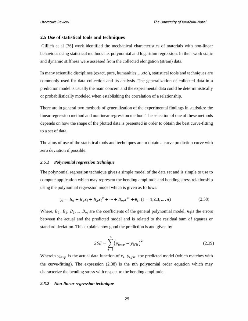
2.5.1 Polynomial regression technique
The polynomial regression technique gives a simple model of the data set and is simple to use to
compute application which may represent the bending amplitude and bending stress relationship
using the polynomial regression model which is given as follows:
𝑦𝑖 = 𝐵0 + 𝐵1𝑥𝑖 + 𝐵2𝑥𝑖2 + ⋯ + 𝐵𝑚𝑥𝑚 +∈𝑖, (𝑖 = 1,2,3, … , 𝑛) (2.38)
Where, 𝐵0, 𝐵1, 𝐵2, … , 𝐵𝑚 are the coefficients of the general polynomial model, ∈𝑖is the errors
between the actual and the predicted model and is related to the residual sum of squares or
standard deviation. This explains how good the prediction is and given by
𝑆𝑆𝐸 = ∑(𝑦𝑖𝑒𝑥𝑝 − 𝑦𝑖𝑓𝑖𝑡)2
𝑛
𝑖=1
(2.39)
Wherein 𝑦𝑖𝑒𝑥𝑝 is the actual data function of 𝑥𝑖, 𝑦𝑖,𝑓𝑖𝑡 the predicted model (which matches with
the curve-fitting). The expression (2.38) is the nth polynomial order equation which may
characterize the bending stress with respect to the bending amplitude.
2.5.2 Non-linear regression technique

Literature Review The University of KwaZulu-Natal
26
Non-linear regression modelling are often used and considered to have more scientific
significance than the previous technique. The mathematical expression most commonly used is
described by the power series as follows:
𝑦𝑖 = 𝑎𝑥𝑖𝛼 𝑄(𝑥𝑖) (2.40)
Where 𝑎 and 𝛼 are the function parameter depends on the material characteristics. From a
linearized form linearized, equation (2.40) initially represented the log-log scale where 𝑎 is the
antilog of the intercept resulting from intersection of the curve plot in log-log scale with y-axis
illustrated in the equation (2.41), 𝛼 is the slope and 𝑄(𝑥𝑖) is the factor of correction. In the work
done by Newman [39], this factor was reviewed and modelled according to the regression model
transformation which is based on equation (2.41)
log 𝑦𝑖 = 𝛼 𝑙𝑜𝑔𝑥𝑖 + log 𝑎 + 𝜖𝑖 (2.41)
Where 𝜖𝑖 is the random error which is a parameter in the correction factor 𝑄(𝑥𝑖) equation (2.41)
and after transformation when using the simple logarithm gives the following expression:
𝑦𝑖 = 𝑎𝑥𝑖𝛼10𝜖𝑖 (2.42)
Considering here that the regression was based on the natural logarithm transformation curve, the
equation (2.42) becomes:
𝑦𝑖 = 𝑎𝑥𝑖𝛼𝑒𝜖𝑖 (2.43)
The correction factor by identification function is related to 𝑄(𝑥𝑖) = 10𝜖𝑖 and 𝑄(𝑥𝑖) = 𝑒𝜖𝑖. At
this stage, the main concern is to find out among those two correction factors which is more
suitable to use which will give a good approximation of the prediction that is close to the
experimental data.
The random errors are given by the half of the mean of errors from the regression when using the
simple logarithm which is described as follows:
10∈ = 10𝑀𝑆𝐸
2 (2.44)
MSE is the mean square of the errors from the regressions. If the residual errors are normally
distributed, then the MSE may be calculated indicated in equation:

Literature Review The University of KwaZulu-Natal
27
𝑀𝑆𝐸 = ∑(𝑦𝑖𝑒𝑥𝑝 − 𝑦𝑖𝑓𝑖𝑡)2
𝑁 − 2
𝑁
𝑖=1
(2.45)
Where N is the number of pairs and 𝑦𝑖𝑒𝑥𝑝 − 𝑦𝑖𝑓𝑖𝑡 are the residual errors
On the other, when the residual errors are not normally distributed the equation (2.45) becomes:
𝑀𝑆𝐸 = ∑(𝑦𝑖𝑒𝑥𝑝 − 𝑦𝑖𝑓𝑖𝑡)2
𝑁
𝑁
𝑖=1
(2.46)
Regardless of the type of correlation or the normality of the residuals, the estimation of the
correction factor is obtained. The predicted stress values may then be obtained from the equation
(2.41) or equation (2.42) by a using correction factor (estimates of 10∈) from equation (2.44).
2.6 Summary
Many laboratory works are presented by various researchers who wanted to validate or verify the
analytical and numerical models.
It is well known that laboratory apparatus and test arrangements can be quite different from each
other. Some experiments are performed with the rigid clamp and other are using commercial
clamp with different sag angles. The comparison between two different experimental works is
usually not appropriate because many parameters must be taken into account.
From the analytical approach of PS formula to the experimental work, there are discrepancies
because the calculated stress, which is an idealized stress, and the measured stress, which is the
actual stress [20]. The analytical approach is based on many assumptions which can be the cause
of deviation from the measured stress (strain).
Various approaches [21] were used to solve this problem using empirical bending stiffness but
none of them achieved wide acceptance [2].
Many deeper works are currently in progress in order to quantify the real stress from experimental
work. This will allow improving the results obtained using the analytical PS formula that depends

Literature Review The University of KwaZulu-Natal
28
strongly on the bending stiffness [20] and evaluating the non-linearity at small amplitudes in this
formula.
Based on the elaborated theories such as PS formula, the bending stiffness mechanism model of
Papailiou, including the experimental approach which will be performed in this study, a model
could be developed. The new model will give a real stress through a correspondent bending
stiffness and will be used on the conductor with the same number of layers and at different range
tension each.
In many disciplines, the experimental approach and statistical analysis have showed giving a good
prediction of the event of mechanical characteristics with non-linear behaviors. Claren and Diana
[14] noticed that the experimental curve is non-linear and this was observed in the most
conductors tested. In these conditions, statistical technique may be the unique solution to
accurately express the mechanical behavior of conductor under alternated motion.

The University of KwaZulu-Natal
29
CHAPTER 3
EXPERIMENTAL EQUIPMENT AND PROGRAMME
3.1 Background
The Vibration Research and Testing Centre (VRTC) research unit has been initiated in 2004 as
the result of the partnership between ESKOM and University of KwaZulu-Natal. The purpose of
the VRTC is to accompany ESKOM in its power line studies and research development.
The main objective of this work was to collect the stress/strain obtained in relation to the
amplitude between 0.01 mm, and 1.2 mm of four different suspended overhead lines common
used in ESKOM transmission lines and each conductor at three different levels of tension (as
percentage to its Ultimate Tensile Strength (UTS)).
In this chapter, the material used, laboratory set up and equipment, as well as the experimental
procedures and methodology are presented according to international recommendations and
standards. In addition, an overview of the design of a new loading arm is given.
3.2 Laboratory configuration and equipment
In this section, the laboratory configuration and different equipment used for this research are
described.
3.2.1 General
The VRTC’s bench consists of an 84.5 m span length of conductor, supported by rigid clamps,
which are fixed on two concrete blocks adequately designed to absorb the vibration during the
test as presented in figure 3-1. An electrodynamic shaker was placed at 1.2m away from the
tension end concrete block to simulate the wind input force on the conductor which is illustrated
in figure 3-2. More details of the laboratory test arrangement are reported [30].
In accordance with the international and national standards, the VRTC lab has been designed to
perform the experiments at the recommended temperatures between 19.5℃ and 21.5℃, for this
reason six powerful air conditioners were disseminated along the laboratory and these are
monitored by using the thermocouples surrounding the entire conductor bench. The test

Experimental Equipment and Programme The University of KwaZulu-Natal
30
arrangement of the VRTC laboratory is illustrated in figure 3-1
Figure 3-1 Test arrangement of conductor at VRTC
Two shaker control systems were used for the tests: The Vibration Interactive Program (VIP) and
the PUMA control system. With the VIP control system the first system presents advantages since
the output parameters i.e. amplitudes and velocities are manually controlled by adjusting the
excitation voltage to shaker. The control is done by using a function generator (Agilent 33220A)
that is connected to the amplifier of the shaker with measurements taken using the Lab View
software (National Instrumentation). Figure 3-2 illustrated Electrodynamic vibration exciter:
shaker and rigid connection:
Figure 3-2 Electrodynamic vibration exciter: shaker (left) and rigid connection (right)
Concrete
block
Concrete
block
Rigid clamp Rigid clamp
Tension clamp
Termination
clamp
Active span 84.6 m
Conductor Shaker
Rigid connection
Accelerometerrs
Strain gauges Constant tension
device
Transducer
Air conditioning
Experimental Equipment and Programme The University of KwaZulu-Natal
31
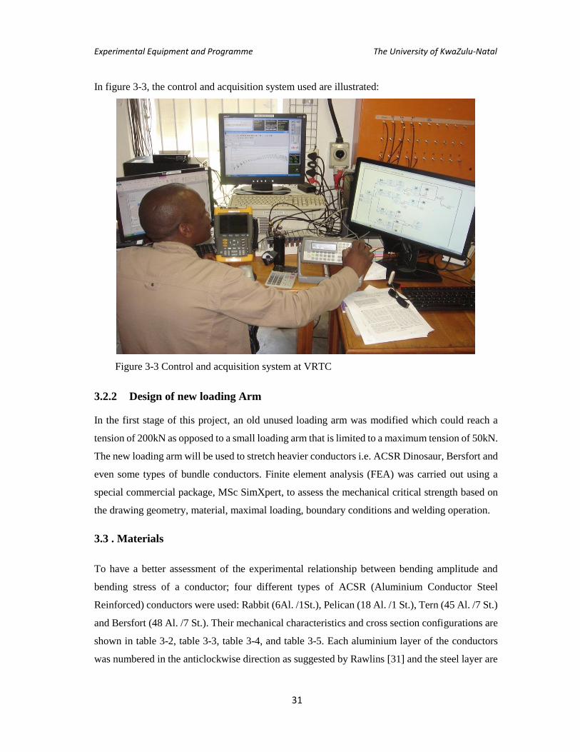
In figure 3-3, the control and acquisition system used are illustrated:
Figure 3-3 Control and acquisition system at VRTC
3.2.2 Design of new loading Arm
In the first stage of this project, an old unused loading arm was modified which could reach a
tension of 200kN as opposed to a small loading arm that is limited to a maximum tension of 50kN.
The new loading arm will be used to stretch heavier conductors i.e. ACSR Dinosaur, Bersfort and
even some types of bundle conductors. Finite element analysis (FEA) was carried out using a
special commercial package, MSc SimXpert, to assess the mechanical critical strength based on
the drawing geometry, material, maximal loading, boundary conditions and welding operation.
3.3 . Materials
To have a better assessment of the experimental relationship between bending amplitude and
bending stress of a conductor; four different types of ACSR (Aluminium Conductor Steel
Reinforced) conductors were used: Rabbit (6Al. /1St.), Pelican (18 Al. /1 St.), Tern (45 Al. /7 St.)
and Bersfort (48 Al. /7 St.). Their mechanical characteristics and cross section configurations are
shown in table 3-2, table 3-3, table 3-4, and table 3-5. Each aluminium layer of the conductors
was numbered in the anticlockwise direction as suggested by Rawlins [31] and the steel layer are

Experimental Equipment and Programme The University of KwaZulu-Natal
32
coloured in blue. ACSR conductor are composed of one or more layers of hard-drawn
concentrically-stranded type 1350 H19 aluminium wire with a high-strength galvanized steel
core. The core could contain one or many steel wires (1, 7, and 19). These conductors are actually
among the most used by ESKOM in low voltage (LV), medium voltage (MV), high voltage (HV)
and extra high voltage (EHV) and are manufactured in South Africa. Examples of commonly used
conductor in HV and EHV in South Africa are shown in table 3-1 (ESKOM’s transmission line
map)
Table 3-1: example of the commonly used conductors in HV and EHV in South Africa
Conductor
Type
Distance
km Start Name End Name Design Volt
4 Pelican 17.19 Grassridge Poseidon 220kV
4 Pelican 115.13 Dedisa Poseidon 400kV
6 Tern 429.48 Gamma Perseus 765kV
3 Tern 406.80 Beta Delphi 400kV
3 Tern 285.05 Arnot Maputo 400kV
3 Tern 246.07 Droerivier Hydra 400kV
2 Bersfort 173.04 Athene Pegasus 400kV
3 Bersfort 119.17 Ariadne Venus 400kV
3 Bersfort 112.47 Camden Duvha 400kV
3 Bersfort 154.70 Majuba Pegasus 400kV
In South Africa, Tern and Bersfort conductors are the most commonly used transmission line
conductors and are used in different configuration i.e. single and bundle (twin, triple…). It is
important to underline that Tern conductor are the most used in kilometres of conductor and in
high voltage and Extra High Voltage(EHV) between 400 and 765 kV. Four conductors were
chosen for this study: Two conductors Rabbit and Pelican having a single steel core and the other
two Tern and Bersfort having a steel core with seven steel wires. It is indeed a good scenario to
explore the effect of conductor sizes for those categories of conductors in order to assess the
distribution of stress when the amplitude is varying on many steel wires (1, 7, and 19). It is

Experimental Equipment and Programme The University of KwaZulu-Natal
33
necessary to emphasise that ACSR Rabbit conductor is used in Mean Voltage (MV) and it is why
it is not in listed table 3-1.
The minimum stiffness of different conductors are given in table 3-2, table 3-3, table 3-4, and
table 3-5 was calculated using equation (2.28). All other parameters .i.e. diameter, number of
wires, linear mass, and the rated tensile strength, have been given by the supplier (Aberdare cable)
and by EPRI [2].
Table 3-2 Mechanical characteristic and cross section of ACSR Rabbit (18 Al. / 1 St.) conductor
Total area (mm2) 8.81
Overall diameter (mm) 10.05
Number of strand per layer
- Steel
- Aluminium
1
6
Ø of Aluminium wire (mm) 3.35
Ø of Steel wire (mm) 3.35
Linear Mass (kg/m) 0.214
Rated Tensile Strength (N) 18 500
Conductor Stiffness (Nm2) 12.21
Table 3.3 Mechanical characteristic and cross section of ACSR Pelican (18 Al. /1 St.) conductor
Total area (mm2) 255.77
Overall diameter (mm) 20.68
Number of strand per layer
- Steel
- Aluminium
1
12 - 6
Ø of Aluminium wire (mm) 4.14
Ø of Steel wire (mm) 4.14
Linear Mass (kg/m) 0.771
Rated Tensile Strength (N) 52 490
Minimum Stiffness (Nm2) 20.78

Experimental Equipment and Programme The University of KwaZulu-Natal
34
Table 3.3 Mechanical Characteristics and cross section of ACSR Tern (45 Al. /7 St.) conductor
Total area (mm2) 430.71
Overall diameter (mm) 27
Number of strand per layer
- Steel
- Aluminium
6 -1
21-15-9
Ø of Aluminium wire (mm) 3.38
Ø of Steel wire (mm) 2.25
Linear Mass (kg/m) 1.334
Rated Tensile Strength (N) 98 310
Minimum Stiffness (Nm2) 21.60
Table 3.4 Mechanical characteristics and cross section of ACSR Bersfort (48 Al. /7 St.)
conductor
Total area (mm2) 746.9
Overall diameter (mm) 35.56
Number of strand per layer
- Steel
- Aluminium
6-1
22-16-10
Ø of Aluminium wire (mm) 4.27
Ø of Steel wire (mm) 3.32
Linear Mass (kg/m) 2.37
Rated Tensile Strength (N) 180 100
Minimum Stiffness (Nm2) 62.76
3.4 Experimental Methodology
Based on many assumptions the PS formula [2] gives the relationship between the bending
amplitude and bending stress/strain on the uppermost wire of the conductor at the point where the
conductor enters, or becomes restrained by, the clamp. This nominal stress determined by PS
formula is an idealized stress because it relies on many assumptions .i.e. the cable is considered
as a rod, but in reality it is constituted by the helical structure (constituted of twisted wires).
Analysis of the dynamic stress at these supports is complicated because due to the stranded
configuration of the conductors during bending the conductor cross section does not remain plane
[16].

Experimental Equipment and Programme The University of KwaZulu-Natal
35
This work is mainly intended to collect data from different ACSR conductors at different levels
of tensile loads (in relation to their ultimate tensile strength (UTS)) and then to provide a realistic
model by statistically analysing those collected data (regression) in order to better assess the stress
(strain) as a function of bending amplitude. Statistical analysis is commonly used in several
research fields using various analysis models of regression i.e. linear, non-linear and polynomial.
The choice of the listed regression is related to fitting the best curve to the data results [32]. It is
well recognised that the polynomial regression is much easier to program even though often found
difficult to interpret. Also the power series model regressions were carried out and showed a very
good fit in many research disciplines.
IEEE standard [13] and CIGRE recommendations [28] suggest investigating the strains localized
on top of the surface of the conductor at the edge of the rigid clamp (at the o-called last point of
contact), where the fretting fatigue mostly happens (high stress part). The amplitude sensor for
displacement measurement is suggested to be placed at 89 mm (𝑥𝑏) from the clamp edge. This
suggestion was initiated by Tebo [12] for the reason that at this distance, the shape of the
conductor was governed only by the stiffness characteristic not by the inertial force induced by
the acceleration in the loops.
The experimental analysis of the dynamic stresses measured on the uppermost wire of the outer
strand layer is considered in the PS model. The experimental stresses thus collected, should
provide a realistic model (analytical or deterministic model) after statistical analysis. This model
was established for three different level of tension that can be determined by using strain gauge
measurements associate with Hooke’s Law which gives the correlation between strain and stress
illustrated in the equation (3.1).
𝜎𝑏 = 𝐸. 휀𝑏 (3.1)
The stress results, that were initially collected as strains were explored by using equation (3.1),
because the stress data gives an insight of the fatigue failure (nominal stress).
3.4.1 Measurements of elongations (strain)
The strains in question have very low values and must be recorded from the far ends of the
laboratory and at the frequency of the vibration system. For this reason a strain measurement
system was used which is constituted of:
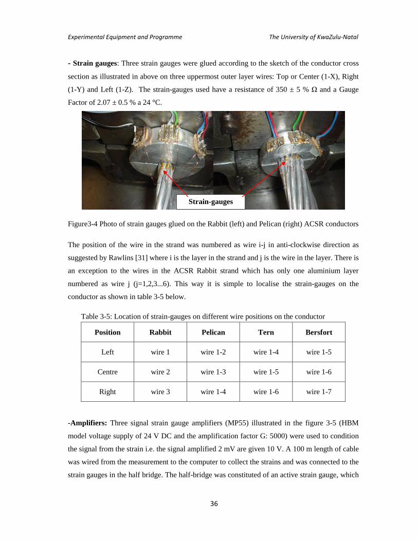
Experimental Equipment and Programme The University of KwaZulu-Natal
36
- Strain gauges: Three strain gauges were glued according to the sketch of the conductor cross
section as illustrated in above on three uppermost outer layer wires: Top or Center (1-X), Right
(1-Y) and Left (1-Z). The strain-gauges used have a resistance of 350 ± 5 % Ω and a Gauge
Factor of 2.07 ± 0.5 % a 24 °C.
Figure3-4 Photo of strain gauges glued on the Rabbit (left) and Pelican (right) ACSR conductors
The position of the wire in the strand was numbered as wire i-j in anti-clockwise direction as
suggested by Rawlins [31] where i is the layer in the strand and j is the wire in the layer. There is
an exception to the wires in the ACSR Rabbit strand which has only one aluminium layer
numbered as wire j (j=1,2,3...6). This way it is simple to localise the strain-gauges on the
conductor as shown in table 3-5 below.
Table 3-5: Location of strain-gauges on different wire positions on the conductor
Position Rabbit Pelican Tern Bersfort
Left wire 1 wire 1-2 wire 1-4 wire 1-5
Centre wire 2 wire 1-3 wire 1-5 wire 1-6
Right wire 3 wire 1-4 wire 1-6 wire 1-7
-Amplifiers: Three signal strain gauge amplifiers (MP55) illustrated in the figure 3-5 (HBM
model voltage supply of 24 V DC and the amplification factor G: 5000) were used to condition
the signal from the strain i.e. the signal amplified 2 mV are given 10 V. A 100 m length of cable
was wired from the measurement to the computer to collect the strains and was connected to the
strain gauges in the half bridge. The half-bridge was constituted of an active strain gauge, which
Strain-gauges

Experimental Equipment and Programme The University of KwaZulu-Natal
37
was glued on the wire and a dummy strain-gauge placed on a separate aluminum plate (with the
same characteristic as the measuring wire) for temperature compensation. The MP55 amplifier is
constituted of a filter module which is useful for filtering the overflow signal and interference
(noise). A virtual filter from LabView was used associated to the physical filter incorporated in
the MP55 (100 Hz) which also aims to prevent aliasing such as the shift of zero reading.
-Data acquisition (DAQ) device: The type of DAQ used is a brand of National Instruments (NI)
that constituted of a chassis (card) for input data into the computer and two NI 9233 modules each
having 4 differential analogue inputs ( rate of sampling 52 kilo samples/sec and a resolution of
24 bits). One module was allocated for the strain measurements and the other for acceleration and
displacements measurements as illustrated in figure 3-5.
Figure 3-5 Data acquisition- NI 9233 modules (Left) and signal amplifier MP55 (right)
-Wirings: In order to prevent signal losses and interferences, a special kind of cable is used to
transfer signals from different points of measurement (strain-gauges and accelerometer as
displacement transducers) was used. From the strain-gauges to the amplifier, ordinary electrical
cables could be used for the short distance. Due to the distance between the computer and the
amplifier, the coaxial cables (MIL-C-17F-RG 058) were used for the displacement transducer and
the strain-gauge MP55 meters which cable of low resistance since the cable is of 100 m length.
-Computer: The shaker controller and data acquisition was accomplished using a commercial
package .i.e. NI LabView and Signal Express driver, allowing the real-time processing signal and

Experimental Equipment and Programme The University of KwaZulu-Natal
38
storing of data. Virtual digital filters were placed in the block diagram in order to clean up the
noisy signals i.e. interference due to the electromagnetic field of equipment. These filters were
used for accelerometer and strain-gauges since the value picked are at low amplitudes (low signal
which is easy to be influenced by the interference). The principle of measurement using the strain-
gauges illustrated by the schematic in figure 3-6:
Figure 3-6 Block diagram of strain measurements showing: active 휀𝑎 and dummy 휀𝑐 strain-
gauges, the amplifier, wirings and the computer
3.4.2 Experimental Procedures
In order to minimise possible errors due to the measurements, the experimental procedures were
conducted according to International Standard (IEEE and IEC), and recommendations (CIGRE).
It is thus important to underline that the VRTC Lab is designed to perform the testing with
0 0 0 0
Digital
display
Recorde
r
Strain gages (Half-bridges)
Completion Circuit
Gain
Power supply 24 V DC
Sensor Matching circuit Output
Amplifier MP55
Computer
Smart signal
conditioning
A D
D A
εc
εa

Experimental Equipment and Programme The University of KwaZulu-Natal
39
constant temperature (between 19.5 ℃ and 21.5 ℃) since six powerful air conditioners are
installed along the conductor bench and are controlled internally and measurements are done by
eight suspended thermocouples disseminated on the length of the conductor.
3.4.2.1 Installation of the conductor on the bench
Conductors were donated by Aberdare cables and were brought on drums. The conductor was
opened, then stretched and conditioned for 35 % UTS for more than one night since the conductor
was rolled up for quite a long time on the drum. To attach the conductor on both sides, pistol grips
were used for the Rabbit and Pelican which is illustrated by figure 3.3, and dead-ends used for
Tern and Bersfort conductor.
Figure 3-7 Photo of pistol grip; Pelican (left) and dead-end clamp: Bersfort (right)
For the two other bigger diameter size conductors, a dead-end clamp was used to grip the
conductor using the relevant procedure underlined in the IEC standards [37]. The advantage of
using the crimped dead-end in the laboratory work is to avoid the internal layers to slip during the
loading procedure as opposed using the pistol grip especially for bigger diameter conductors. An
automatic hydraulic crimping machine (IZUMI) was used for crimping the dead-end on the
conductor, starting by the steel core layer itself and then both steel and aluminium layers were
crimped together. Several dies were used in the crimping machine according to the type, diameter
and size of the conductor).
Rigid clamps placed on the concrete blocks (figure 3-1) are designed to be tightened with four
bolts at a torque of ± 52 Nm based on IEC recommendations [1] and rigidly fixes the conductor
Pistol grip Dead-end clamp

Experimental Equipment and Programme The University of KwaZulu-Natal
40
by compression of the keeper on the base of the rigid clamp. An aluminium insert was used for
each conductor diameter size in the rigid clamp.
3.4.2.2 Strain-gauges and accelerometers on the conductor
The objective is to glue the strain gauges at the location where the most significant strain occurs.
The first position susceptible to get the highest strain is on the top of the last point of contact
(LPC: the edge of the clamp) which is considered as the reference in the PS calculations. The
strain gauges were inspected before and after they were glued on the conductor. The inspection
was aimed at assuring that the gauges were not broken or to make sure that the resistance value
of the extensometer used is 350 ± 1.5 Ohms.
Two accelerometers were placed on the conductor: one at 89 mm from the LPC and the other one
at the shaker position with respectively sensitivities of 97.2 mV/g and 96.7 mV/g. It was observed
in the all cases that the resonance frequencies were found during the experiments when the ratio
on the amplitudes of the shaker 𝑌𝑠 and that on the 89 mm bending amplitude 𝑌𝑏 equal or smaller
than six, i.e.:
𝑦𝑠𝑦𝑏
⁄ ≤ 6 (3.2)
3.4.3 Dynamic Measurements
.4.3.1 Choice of bending amplitude peak-to-peak(mm)
Based on the CIGRE safe line design it is recommended to investigate the amplitudes between
0.2 mm and 1.2 mm [28]. In addition, the amplitudes between 0.01 mm and 0.1 mm were
investigated because of the uncertainty of the P-S formula at small amplitudes. From these
amplitudes, a non-linearity curve of stress results were observed on the ACSR Drake conductor
by Poffenberger-Swart [2] which stated that the small amplitudes were in the cloudy region
because, it could not be adequately represented by their formula.
Some particular amplitudes were chosen in order to compare with some previous results with past
research i.e. work on ACSR Ibis (done by Aida and co-worker), ACSR Bersfort by Levesque et
al conductor which has the characteristic almost close to the ACSR Pelican and Papailiou on the
ACSR Cardinal [17].
.4.3.2 Choice of the static loading (% UTS)
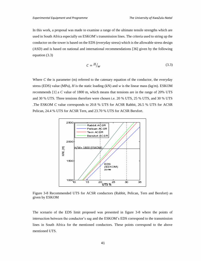
Experimental Equipment and Programme The University of KwaZulu-Natal
41
In this work, a proposal was made to examine a range of the ultimate tensile strengths which are
used in South Africa especially on ESKOM’s transmission lines. The criteria used to string up the
conductor on the tower is based on the EDS (everyday stress) which is the allowable stress design
(ASD) and is based on national and international recommendations [36] given by the following
equation (3.3)
𝐶 = 𝐻𝑤⁄ (3.3)
Where C the is parameter (m) referred to the catenary equation of the conductor, the everyday
stress (EDS) value (MPa), H is the static loading (kN) and w is the linear mass (kg/m). ESKOM
recommends [1] a C value of 1800 m, which means that tensions are in the range of 20% UTS
and 30 % UTS. Three tensions therefore were chosen i.e. 20 % UTS, 25 % UTS, and 30 % UTS
.The ESKOM C value corresponds to 20.8 % UTS for ACSR Rabbit, 26.5 % UTS for ACSR
Pelican, 24.4 % UTS for ACSR Tern, and 23.70 % UTS for ACSR Bersfort.
Figure 3-8 Recommended UTS for ACSR conductors (Rabbit, Pelican, Tern and Bersfort) as
given by ESKOM
The scenario of the EDS limit proposed was presented in figure 3-8 where the points of
intersection between the conductor’s sag and the ESKOM’s EDS correspond to the transmission
lines in South Africa for the mentioned conductors. These points correspond to the above
mentioned UTS.
UTS %
H/W= 1800 (ESKOM)
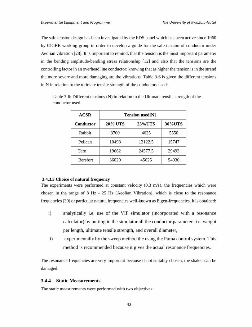
Experimental Equipment and Programme The University of KwaZulu-Natal
42
The safe tension design has been investigated by the EDS panel which has been active since 1960
by CIGRE working group in order to develop a guide for the safe tension of conductor under
Aeolian vibration [28]. It is important to remind, that the tension is the most important parameter
in the bending amplitude-bending stress relationship [12] and also that the tensions are the
controlling factor in an overhead line conductor: knowing that as higher the tension is in the strand
the more severe and more damaging are the vibrations. Table 3-6 is given the different tensions
in N in relation to the ultimate tensile strength of the conductors used:
Table 3-6: Different tensions (N) in relation to the Ultimate tensile strength of the
conductor used
ACSR Tension used[N]
Conductor 20% UTS 25%UTS 30%UTS
Rabbit 3700 4625 5550
Pelican 10498 13122.5 15747
Tern 19662 24577.5 29493
Bersfort 36020 45025 54030
3.4.3.3 Choice of natural frequency
The experiments were performed at constant velocity (0.3 m/s). the frequencies which were
chosen in the range of 8 Hz - 25 Hz (Aeolian Vibration), which is close to the resonance
frequencies [30] or particular natural frequencies well-known as Eigen-frequencies. It is obtained:
i) analytically i.e. use of the VIP simulator (incorporated with a resonance
calculator) by putting in the simulator all the conductor parameters i.e. weight
per length, ultimate tensile strength, and overall diameter,
ii) experimentally by the sweep method the using the Puma control system. This
method is recommended because it gives the actual resonance frequencies.
The resonance frequencies are very important because if not suitably chosen, the shaker can be
damaged.
3.4.4 Static Measurements
The static measurements were performed with two objectives:
Experimental Equipment and Programme The University of KwaZulu-Natal
43
i) to check on how the stress varies from the low to high UTS,
ii) to assess the stress induced by the rigid clamp pressure imparted when
tightening it.
It was thus tested firstly with the clamp tightened at 52 Nm following the recommendations and
secondly with clamps loosened as performed in the previous work [30]. The conductor was
tensioned at the lowest possible tension (when the sagging conductor soft touches the floor) and
thereafter the strain-gauge meters were zeroed.
3.5 Experimental Analysis
The objective is to reduce possible errors which may occur during experimental measurement and
which may due by the noisy signals (interferences). The choice of a reliable experimental analysis
is necessary in order to minimize those possible errors for this project which depends on the
experimental outputs.
3.5.1 Static strain analysis
The sensitivity for the strain-gauge is 2 mV/V with sensitivity at 400 /V from the amplifier.
This is considered in the strain amount read 휀𝑟𝑒𝑎𝑑on the computer having in mind that the signal
of the strain-gauges collected in voltage has been amplified and is given by the equation (3.4).
휀 ≈4𝑉𝑜𝑢𝑡
𝑉𝑒𝑥𝑐𝐺𝑓
106
𝐾𝑓 (3.4)
where 𝑉𝑜𝑢𝑡 is the voltage drop at the bridge sensor, 𝑉𝑒𝑥𝑐 is the voltage of excitation, 𝐺𝑓 is the
gauge factor which is equal to 2.07 and 𝑘𝑓 is the amplifier factor which is equal 5000. The amount
of 106 is multiplied in the equation in order to have the measurement in microstrains. To eliminate
as possible errors due to the noise in the measurement, the average was determined after three
measurements were performed using the equation (3.5).
Ԑ𝑠 =∑ 휀𝑠,𝑖
𝑁𝑖=1
𝑁
(3.5)

Experimental Equipment and Programme The University of KwaZulu-Natal
44
3.5.2 Dynamical strain analysis
The measurement of the strain due to bending is determined by the peak to peak amplitude which
gives the maximum and the minimum strains defined by the plot “strain as a function of time”
which is shown in seconds in the figure 3-9. This was respectively positive and negative according
to the principle of traction and compression. The mean 휀𝑏𝑖 was calculated for each period in time
and is considered equal for every second and then the average over 60 seconds was determined
and given by the equation (3.6)
휀𝑏𝑖 =∑ (휀𝑏𝑗,𝑚𝑎𝑥
𝑁𝑗=1 − 휀𝑏𝑗,𝑚𝑖𝑛)
2
(3.6)
Where 휀𝑏𝑛,𝑚𝑎𝑥 and 휀𝑏𝑛,𝑚𝑖𝑛 are respectively the maximum and the minimum strains collected
corresponding to one amplitude peak-to-peak, and which are most closely equivalent |휀𝑏𝑛,𝑚𝑎𝑥| ≃
|휀𝑏𝑛,𝑚𝑖𝑛| (traction and compression). The strain curve as a function of time is showed in the figure
3-9 and is defined by the shape of a sinusoidal function. For more accurate results, the experiment
was conducted at each amplitude level and performed at least three times in order to minimize the
errors due to the measurement. The bending strain Ԑ𝑏 thus present is the average strain of n
measurements of strains collected (휀1 , 휀2, 휀3, … , 휀𝑛 𝑎𝑛𝑑 𝑛 = 1,2,3, … ) at each amplitude level.
Ԑ𝑏 =∑ 휀𝑖
𝑁𝑖=1
𝑁
(3.7)
Equation (3.3) is used to validate the experimental measurement and to verify the reliably of the
instruments used which were calibrated before the experimental work.

Experimental Equipment and Programme The University of KwaZulu-Natal
45
Figure 3-9 Figure strain vs. time curve during a bending strain measurement on ACSR Tern
conductor at an amplitude of 0.1 mm peak-to-peak
During the dynamic measurement, the strain-gauges were read continuously whilst being loaded,
and then it is evident that non-uniformities in the strain signal occurred. To overcome this, several
measurements were performed for the reason to limit uncertainty and errors; the related bending
stress 𝜎𝑏 is obtained using the expression (3.1).
The strain due to the temperature was not considered according to the assumption taken in the
first chapter about the variation of temperatures. Although the ambient temperature along the
conductor in the laboratory is maintained constant close to 21 ℃ (± 1 ℃) as recommended by the
measurement standard, a temperature compensated strain-gauge and also the preventive device
was employed to eliminate the thermal effect, otherwise errors in the measurements may occur.
The frequencies from both the measurements and the conductor-shaker system should be
synchronised whereby sinusoidal wave form is obtained. The manufacturer of the LabView
package [35] suggested choosing a minimum sampling frequency which is the sampling rate ƒ𝑠
(number of samples per second) defined to be greater than ten times the frequency of the system
to measure. Levesque’s research [33] suggested that this frequency has to be equal to the spectral
frequency (∆ƒ ≈ 0.1) multiplied by the number of points as described in the equation (3.8).
0 0.1 0.2 0.3 0.4 0.5 0.6 0.7 0.8 0.9-80
-60
-40
-20
0
20
40
60
80
Time
Ben
din
g S
train
[M
icro
stra
ins]
Min
Max

Experimental Equipment and Programme The University of KwaZulu-Natal
46
ƒ𝑠 = 𝑁𝑢𝑚𝑏𝑒𝑟 𝑜𝑓 𝑝𝑜𝑖𝑛𝑡𝑠 × ∆ƒ
(3.8)
Indeed, as the strain recorded as function of the peak-to-peak amplitude 2500 samples have been
recorded for each second at a rate of 5000 Hz.
3.5.3 Identification of appropriate statistical regression technique
To identify the appropriate statistical regression technique, the step should be followed:
- Step 1: the variables collected are plotted in a scatter-diagram Bending stress 𝜎𝑎 as
function of bending amplitude 𝑦𝑏.The relationship between two variables is represented
in the graph.
- Step 2: observing the scatter shape curve which is a form of existing relationship model
shape, the type of regression technique is chosen among the several predefined in the
package. Three factors have to be:
- i) the estimator or predictor factor 𝑅2 which has to be 𝑅2 ≅ 1 (strength of the relationship),
- ii) the standard deviation SSE between the result and the prediction model and
- iii) the model of stress distribution on which the standard error depends.
There are several statistical analysis methods which are used for the prediction of the experimental
result. The appropriate model should:
(i) give a good correlation with the results and
(ii) depend on decision of the researcher i.e. expected applications and analysis.
In most of the cases, it is a compromise between the above. Other concerns in statistical prediction
are its limitation: the results can be valid for the values between the points tested.
In figure 3-10 the flowchart showing different step for prediction with statistical regression
technique.

Experimental Equipment and Programme The University of KwaZulu-Natal
47
Figure 3-10 Flowchart showing step of model prediction using statistical regression technique
START
Step 1: Plot (𝑦𝑏, 𝜎𝑏)
Step2: choice of
type regression
model
Check
The Estimator
Parameter
𝑅2 ≅ 1
If not 𝑅2 ≅ 1
And return to
step2 If 𝑅2 ≅ 1
Return to step 2
Yes
Check
If the prediction
Model is
Ambiguous
Evaluate the Mean
standard errors (MSE)
and the frequency of
distribution
No
END
Check If the stresses are
normally distributed
No
Yes
If yes use the error = half
of the root square MSE
with
𝑀𝑆𝐸
= ∑(𝑦𝑖𝑒𝑥𝑝 − 𝑦𝑖𝑓𝑖𝑡)2
𝑁 − 2
𝑁
𝑖=1
If not use the error = half of
the root square of MSE
with
𝑀𝑆𝐸
= ∑(𝑦𝑖𝑒𝑥𝑝 − 𝑦𝑖𝑓𝑖𝑡)2
𝑁
𝑁
𝑖=1
Yes No
Experimental Equipment and Programme The University of KwaZulu-Natal
48
3.6 Summary
The procedures of dynamic measurement were performed as follows:
The conductor was well-prepared and was rigidly clamped on the bench at a preloaded tension.
The required tension was then monitored by suitable instrumentation procedures. The strains were
recorded using three different conductor tensions H1, H2 and H3 as a function of the amplitudes
Yb, between 0.01 mm to 1.2 mm which is adjusted manually using the function generator. The
measurement at each amplitude level was repeated at least three times (in order to minimize errors
due to imperfection of signal during measurements). The measurement time was set for 60
seconds at the natural frequency which is close to the resonance frequency was determined by
both the analytical and the sweep method [30]. The data collected were computed and stored for
analysis. Finally the measured strain data have been converted to stress using the Hooke’s law
and plotted, i.e. bending stress as function of bending amplitude.

The University of KwaZulu-Natal
49
CHAPTER 4
EXPERIMENTAL RESULTS
Background
In this chapter, the strain data were collected and plotted as a function of the amplitude. After
calculating the average of the strains there was no significant (± 2 %) difference between the
three measurements. The tests were performed at resonance frequency between 10 Hz and 25 Hz
which were both predicted and measured values. The measurements were carried out according
to the IEEE standard [13] and CIGRE guide [28]. Today, the accuracy of strain-gauges
technology, iteration software, and data acquisition are much better than the ones used in the past.
The strain measured was plotted as a function of the amplitude for each wire and was performed
at different tension levels.
In addition, comparison was done between the results and some prediction models i.e. the
Poffenberger-Swart model and the improved model using the bending stiffness model by
Papailiou [15].
The retained static measurements were compared to the theoretical expression of Ramey and
Townsend [25] that was earlier reported in chapter 2, which gives the axial tension in the strand
and causes an approximate longitudinal static strain of
휀𝑡 =𝐻
(𝑛𝐴𝑠 + 𝐴𝑎)𝐸𝑎
(4.1)
With H = tension in the conductor; 𝐴𝑠 = total area of steel; 𝐴𝑎 = total area of aluminium;
n = modulus of elasticity for steel/modulus of elasticity for aluminium; and Ea = modulus of
elasticity for aluminium. Two equations are commonly used to estimate static bending strains in
conductor strands at the tower support points located at the mouth of a fixed clamp.

Experimental Results The University of KwaZulu-Natal
50
4.2 ACSR Rabbit conductor
In this section, the static and dynamic measurements of the ACSR Rabbit are given:
4.2.1. Static measurement
The conductor was brought to the lowest possible tension of about 2 𝑘𝑁. From this level, the
tension was gradually increased in a step of 0.4 𝑘𝑁 until 4.4 𝑘𝑁. A remarkable difference was
observed in wire 1 with the clamp tightened (CT) and the clamp loosened (CL). One explanation
may be given, because of the static pressure due to the clamping. A torque of 52 kN was used to
clamp the conductor on the bench. On the other two wires, 2 and 3, there was no significant
difference between CT and CL shown in figure 4-1 about ± 15 %.
Figure 4-1 Static strain vs. tension on the three different wires (1, 2, and 3) in the ACSR Rabbit
strand according the sketch in table 3-2
4.2.2. Dynamic measurement
The dynamic strains as illustrated by figure 4-2 presents a general scenario of Rabbit conductor
at three tension levels. from 0.01 mm to 0.2 mm. It was thus noticed that the top wire (wire 2)
provided a smooth growth of data . The exception is observed at 20 % UTS for the amplitude 0.5
mm and 1.2 mm. A simple explanation may be given, is that there is no interference of the top
wire according to the configuration (constituted of two underneath wires: the steel core and the
aluminum wire ). Wire 1 presents irregularity of the strain data in general with exception for the
amplitudes lower than 0.5 mm. As the weight of this conductor is not significant, many ranges of
frequency may be used to perform the bending strain measurement. The resonance frequency
between 10 Hz and 15 Hz were used to get the strain at the fixed amplitude.
2 2.5 3 3.5 4 4.5
-400
-300
-200
-100
0
100
200
300
400
Tension [kN]
Wire 3
Ramey and Townnsend [25]
Clamp Tightened
Clamp Loosened
2 2.5 3 3.5 4 4.5-400
-300
-200
-100
0
100
200
300
400
Tension [kN]
Sta
tic
Str
ain
[ M
icro
str
ain
s]
Wire 1
Ramey and Townsend [25]
Clamped Tightened
Clamp Loosened
2 2.5 3 3.5 4 4.5-400
-300
-200
-100
0
100
200
300
400
Tension [kN]
Wire 2
Ramey and Townnsend [25]
Clamp Loosened
Clamp Tigthened

Experimental Results The University of KwaZulu-Natal
51
Figure 4-2 Dynamic strain vs. Amplitude at 20 % UTS, 25 % UTS and 30 % UTS on the three
different wires (1, 2, and3) in the ACSR Rabbit strand according the sketch in table 3-2
4.3 ACSR Pelican conductor
In this section, static and dynamic measurements on the ACSR Pelican are given:
4.3.1. Static measurements
The static measurement on the ACSR Pelican conductor are almost similar to the results obtained
on the Rabbit conductor. However, there are diffrence in their magnitude and the steps used.
Figure 4-3 shows the static result on the ACSR Pelican conductor.
Figure 4-3 Static strain vs. tension on the three different wires (1, 2, and 3) in the ACSR Pelican
strand according the sketch in table 3-3
0 0.5 10
100
200
300
400
500
600
700
800
Amplitude [mm]
Str
ain
[M
icro
stra
ins]
Wire 1
30%UTS
25%UTS
20%UTS
0 0.5 10
100
200
300
400
500
600
700
800
Amplitude[mm]
Wire 2
20%UTS
25%UTS
30%UTS
0 0.5 10
100
200
300
400
500
600
700
800
Amplitude [mm]
Wire 3
20%UTS
25%UTS
30%UTS
8 10 12 14-400
-300
-200
-100
0
100
200
300
400
Tension [kN]
Sta
tic
Str
ain
[]
Wire 1-2
Ramey and Townsend [25]
Clamp Tightened
Clamp Loosened
8 10 12 14-400
-300
-200
-100
0
100
200
300
400
Tension [kN]
Wire 1-4
Ramey and Townsend [25]
Clamp Tightened
Clamp Loosened
8 10 12 14-400
-300
-200
-100
0
100
200
300
400
Tension [kN]
Wire 1-3
Ramey and Townsend [25]
Clamp Loosened
Clamp Tightened

Experimental Results The University of KwaZulu-Natal
52
4.3.2. Dynamic measurements
In figure 4-4 different plots are given in which the strain as a function of amplitude shown for the
three uppermost wires (wire 1-2, wire 1-3 and wire 1-4) of the Pelican conductor. In general the
result at 20% UTS and 25 % UTS are the same as show by their curve shape in all the wires. The
slip-stick state can be observed in the plots represented in the figure i.e. the strain at 30% UTS is
smaller as compared to the stress at 20% UTS and 25 % UTS. This phenomena is significant in
the wire 1-2 and wire 1-4, while the wire 1-3 the results observed are almost similar for these
different tensions. A simple explanation based on this, is that the stiffness of the ACSR Pelican
is not much affected by the tension
Figure 4-4 Dynamic strain vs. Amplitude at 20 % UTS, 25 % UTS and 30 % UTS on the three
different wires (1-2, 1-3, and 1-4) in the ACSR Pelican strand according the sketch in table 3-3
4.4 ACSR Tern Conductor
In this section, static and dynamic measurements on the ACSR Tern conductor are given:
4.4.1. Static measurements
The pressure of the clamp on the conductor affected the wire 1-5 and wire 1-6 when the tension
varies from 10 𝑘𝑁 to 24.1 𝑘𝑁. These variations are observed between the strain collected when
the clamp is tightened and loosened i.e. at 20.1 𝑘𝑁, which are in magnitude equal to - 67.1 𝜇휀
and 64.7 𝜇휀 for the clamp tightened and the clamp loosened, respectively. The strain observed on
the wire 1-4 indicated no difference for the clamp tightened and the clamp loosened.
0 0.5 10
100
200
300
400
500
600
700
Amplitude [mm]
Str
ain
[M
icro
stra
ins]
Wire 1-2
20% UTS
25% UTS
30% UTS
0 0.5 10
100
200
300
400
500
600
700
Amplitude [mm]
Wire 1-3
20% UTS
25% UTS
30% UTS
0 0.5 10
100
200
300
400
500
600
700
Amplitude [mm]
Wire 1-4
20% UTS
25%UTS
30% UTS

Experimental Results The University of KwaZulu-Natal
53
Figure 4-5 Static strain vs. tension on the three uppermost wires (1-4, 1-5, and 1-6) in the ACSR
Tern strand according the sketch in table 3-4
4.4.2. Dynamic measurements
Comparatively with the two previous conductors, the dynamic strain collected on the Tern
conductor can be clearly observed in figure 4-6. The strains were measured for the amplitudes
less than and equal to 1 mm due to the weight of the conductor and limitations of the shaker.
Figure 4-6 Dynamic strain vs. Amplitude at 20 % UTS, 25 % UTS, and 30 % UTS on the three
different wires (1-4, 1-5, and 1-6) in the ACSR Tern strand according the sketch in table 3-4
4.5 ACSR Bersfort
10 15 20 25-400
-300
-200
-100
0
100
200
300
400
Tension [kN]
Sta
tic
str
ain
[]
Wire 1-4
Ramey and Townsend [25]
Clamp Tightened
Clamp Loosened
10 15 20 25-400
-300
-200
-100
0
100
200
300
400
Tension [kN]
Wire 1-5
Ramey and Townsend [25]
Clamp Tigthened
Clamp Loosened
10 15 20 25-400
-300
-200
-100
0
100
200
300
400
Tension [kN]
Wire 1-6
Ramey and Townsend [25]
Clamp Loosened
Clamp Tightened
0 0.2 0.4 0.6 0.80
100
200
300
400
500
600
Amplitude [mm]
Str
ain
[M
icro
stra
ins]
Wire 1-4
20%UTS
25%UTS
30%UTS
0 0.2 0.4 0.6 0.80
100
200
300
400
500
600
Amplitude [mm]
Wire 1-5
20%UTS
25%UTS
30%UTS
0 0.2 0.4 0.6 0.80
100
200
300
400
500
600
Amplitude [mm]
Wire 1-6
25%UTS
30%UTS
20%UTS

Experimental Results The University of KwaZulu-Natal
54
In This section, static and dynamic measurements on the ACSR Bersfort conductor are given:
4.5.1. Static Measurement
The static measurements with the clamp tightened and with the clamp loosened are similar in
Bersfort conductor, with the exception noticed on the strain result of the wire 1- 4 and on the wire
1-6. On the wire 1-4, there is big difference between the results for the clamp tightened and clamp
loosened with an average deviation of 20 %. A small deviation of about 10% is observed in the
results on the wire 1-6 the tension above 40 𝑘𝑁.
Figure 4-7 Static strain vs. tension on the three uppermost wires (1-4, 1-5, and 1-6) on the ACSR
Bersfort strand according the sketch in table 3-5
4.5.2. Dynamic Measurement
During the dynamic measurements on the ACSR Bersfort conductor, the strain-gauges sinusoidal
signals were clearer than the other conductors that were tested. Due to the weight of the Bersfort
conductor (2.37 𝑘𝑔/𝑚) it was not easy to maintain constant amplitude above 0.8 mm and the
limitation of the shaker since the rigid connection was used. In figure 4-8 the bending strain vs.
bending amplitude is given for different wires 1-4, 1-5 and 1-6. The input resonant frequencies
from the shaker was used for obtaining the amplitude at 89 mm were greater compared to the
previous conductor i.e. at 20 % UTS. The amplitude at the resonance frequency was found at 21
.78 Hz for Bersfort and 19.5 Hz for the Tern conductor.
10 20 30 40 50 60-400
-300
-200
-100
0
100
200
300
400
Sta
tic
Str
ain
[ ]
Wire 1-4
Tension [kN]
Ramsey andTownsend [25]
Clamp Tightened
Clamp Loosened
10 20 30 40 50 60-400
-300
-200
-100
0
100
200
300
400
Tension [kN]
Wire 1-5
Ramsey andTownsend [25]
Clamp Tightened
Clamp Loosned
10 20 30 40 50 60-400
-300
-200
-100
0
100
200
300
400Wire 1-6
Tension [kN]
Ramsey and Townsend [25]
Clamp Tightened
Clamp Loosened

Experimental Results The University of KwaZulu-Natal
55
Figure 4-8 Dynamic strain vs. Amplitude at 20 % UTS, 25 % UTS, and 30 % UTS on the
three different wires (1-4, 1-5, and 1-6) in the ACSR Bersfort strand according the sketch in
table 3-5
Comparison to previous experimental work
There is limited data available in literature regarding the stress measurement on the conductor
used in this research. Levesque et al. [33] performed static and dynamic measurements on ACSR
Bersfort at the univesity of Laval. The conductor was mounted on a bench of 11 m length and
was fastened using a short commercial clamp with an exit angle of 62°. In table 4-1, the
comparison between previous research and this work is shown:
Table 4-1: Comparison between (i)Levesque et al[41], (ii) Ouaki et al [40] and the
present study on Bersfort conductor.
Levesque et al [41] Ouaki et al [43] present work
amplitudes strains-LPC amplitude strains LPC amplitudes strain CE
0.32 157 - - 0.3 223
0.47 231 0.43 200 0.5 304
0.55 264 0.55 300 0.6 370
0.76 357 0.65 330 0.8 439
The LPC is the last point of contact , where the strain-gauge has been glued. The comparison
shows, that the short commercial clamp with the exit angle of 62° reduces the bending strain
between 20%-30% with the variation of the amplitude, even the results seem to be in the same
range level. This can be explained that the radius of curvature of the short commercial clamp
reduces the shear force compared to the squared faced rigid clamp (exit angle equal to 0) used in
0 0.2 0.4 0.6 0.80
50
100
150
200
250
300
350
400
450
Amplitude [mm]
Wire 1-4
20% UTS
25 % UTS
30% UTS
0 0.2 0.4 0.6 0.80
50
100
150
200
250
300
350
400
450
Amplitude [mm]
Str
ain
[M
icro
str
ain
s]
Wire 1-5
20 % UTS
25 % UTS
30% UTS
0 0.2 0.4 0.6 0.80
50
100
150
200
250
300
350
400
450
Amplitude [mm]
Wire 1-6
20 % UTS
25 % UTS
30 % UTS

Experimental Results The University of KwaZulu-Natal
56
this research . Similar conclusions were made by Dalpe [48] in the experimental work for ACSR
Drake and Zebra conductors. which compared two types of clamp with an exit angle of 5° and
10°. McGill et al [10] compared the fatigue performance results between ACSR Drake conductor
attached with four different types of clamp i.e.
(i) short radius and deep groove,
(ii) medium radius and shallow groove,
(iii) medium radius and deep groove, and
(iv) long radius and deep groove.
They concluded that the conductor fatigue performance is reduced when the radius of the clamp
decreases. The figure 4-9 illustrated the different clamps used in [25].
Figure 4-9 Examples of clamps used to compare the performance fatigue of a Drake conductor
Comparison between experimental, P-S and Papailiou Model
The most disseminated and practical model used for design and maintenance purposes
(assessment of life expectancy) is the Poffenberger-Swart formula as noticed in chapter 2 and
given as follows:

Experimental Results The University of KwaZulu-Natal
57
𝜎𝑎 =𝐸𝑎 𝛿 𝑝2
4(𝑒−𝑝𝑥−1+𝑝𝑥)𝑌𝑏 (where 𝑝 = √
𝐻
𝐸𝐽 )
(4.1)
wherein Ea is the Young modulus of aluminium (70 𝐺𝑃𝑎 which is not applied to stranded wires),
𝛿 is the diameter of the outer layer wire (mm), H is the static tension in the conductor (𝑁), 𝐸𝐽 is
the bending stiffness (𝑁. 𝑚𝑚2) and x (89 mm) is the distance from where the amplitude is
measured.
The crucial element in equation (4.1) is the bending stiffness EJ that is normally taken as the
minimum bending stiffness 𝐸𝐼𝑚𝑖𝑛 (constant) as initially developed in the PS model. In the model
developed by Papailiou the bending stiffness is given as a function of the curvature 𝐸𝐽(𝑘) and the
tension in the strand (slip-stick state). The calculation of the varying stiffness is not so easy to use
and it is required to determine the curvature 𝑘 as a function of the amplitude of the conductor
attached at the clamp. The software SEIL has been developed at PFISTERER for the use in the
Vibrec 400 (vibration recorder) which is not public domain used software. This provides the total
stress as function of the amplitude peak-to-peak with as the scenario where the bending stiffness
model of Papailiou is used in the P-S model. Equation (4.2) is also discussed in chapter 2.
𝐸𝐽(𝑘) = 𝐸𝐽𝑚𝑖𝑛 + ∑ 𝐸𝐽𝑠𝑡𝑖𝑐𝑘,𝑗
𝑖−1
𝑗=1
+ (2) ∑ 𝐸𝐽𝑠𝑙𝑖𝑝,𝑗
𝑎
𝑗=1
(4.2)
4.7.1 ACSR Rabbit conductor
The results obtained on different conductors shows that there is a good correlation between the
predicted (Papailiou model) and the experimental results. On the ACSR Rabbit conductor, the
Papailiou model gives an excellent prediction for this conductor stretched at 20 and 25% UTS at
the level range of 0.1 mm to 1.2 mm. At 30 % UTS, and from 0.9 mm to 1.2 mm through the gap
between prediction and experiments becomes significant with the amplitude greater than 0.9 mm.
The deviation between the results and the PS prediction was ±45 % as shown in figure 4-10.

Experimental Results The University of KwaZulu-Natal
58
Figure 4-10 Measured and Predicted (PS Formula and Papailiou Model) of The ACSR Rabbit
conductor at 20 % UTS, 25 % UTS and 30 % UTS
4.7.2 ACSR Pelican conductor In the ACSR Pelican conductor which is illustrated in figure 4-11, it was observed that there is
good correlations with the Papailiou model with the variation of the tension in the strand and the
correlation was better with the measurements from 0 mm to 0.6 mm at 20% UTS, until 0.8 mm
at 25% UTS and 1 mm for 30% UTS. The shape of the data looks similar with the one developed
by Papailiou on the Cardinal conductor [17].
Figure 4-11 Measured and Predicted (PS Formula and Papailiou Model) of The ACSR Pelican
conductor at 20 % UTS, 25 % UTS and 30 % UTS
0 0.5 10
10
20
30
40
50
60
Amplitude p-p [mm]
To
tal
Str
es
s [
MP
a]
ACSR Rabbit 20% UTS
Measured
P-S
Papailiou
0 0.5 10
10
20
30
40
50
60
Amplitude p-p [mm]
ACSR Rabbit 25% UTS
Measured
P-S
Papailiou
0 0.5 10
10
20
30
40
50
60
Amplitude p-p [mm]
ACSR Rabbit 30% UTS
Measued
P-S
Papailiou
0 0.5 10
10
20
30
40
50
60
Amplitude p-p [mm]
ACSR Pelican 25% UTS
Measured
P-S
Papailiou
0 0.5 10
10
20
30
40
50
60
Amplitude p-p [mm]
To
tal
Str
es
s [
MP
a]
ACSR Pelican 20% UTS
Measured
P-S
Papailiou
0 0.5 10
10
20
30
40
50
60
Amplitude p-p [mm]
ACSR Pelican 30% UTS
Measured
P-S
Papailiou

Experimental Results The University of KwaZulu-Natal
59
4.7.3 ACSR Tern conductor In figure 4-12, the stresses collected on the top wire of ACSR Tern conductor correlates well at
20 % UTS from 0.01 mm to 0.7 mm and toward the Poffenberger-Swart prediction model for the
amplitudes greater than 0.7mm. At 25 % UTS, the small amplitudes can be represented by
Papailiou model i.e. from 0.01 mm to 0.2 mm. in contrast to the previous tension, at 30 % UTS
the stresses correlate well enough from 0.04 mm to 1 mm.
Figure 4-12 Measured and predicted (PS Formula and Papailiou Model) of The ACSR Tern
conductor at 20, 25 and 30 % UTS
4.7.4 ACSR Bersfort conductor The measured results correlate well enough with the PS formula except at small amplitude
especially from 0.01 mm to 0.1 mm where the results match with the Papailiou’s model. The
predictions of the stress using the PS model show a deviation of ± 10% (figure 4-13)
Figure 4-13 Measured and Predicted (PS Formula and Papailiou Model) of The ACSR Bersfort
conductor at 20, 25 and 30 % Ultimate Tensile Strength (UTS)
0 0.2 0.4 0.6 0.8 10
5
10
15
20
25
30
35
40
45
Amplitude p-p [mm]
To
tal S
tres
s[N
/mm
2]
ACSR Tern 20% UTS
Measured
P-S
Papailiou
0 0.2 0.4 0.6 0.8 10
5
10
15
20
25
30
35
40
45
Amplitude p-p [mm]
ACSR Tern 25% UTS
Measured
P-S
Papailiou
0 0.2 0.4 0.6 0.8 10
5
10
15
20
25
30
35
40
45
Amplitude p-p [mm]
ACSR Tern 30% UTS
Measured
P-S
Papailiou
0 0.2 0.4 0.6 0.80
5
10
15
20
25
30
35
40
Amplitutude p-p[mm]
To
tal
Str
ess
[N
/mm
2]
ACSR Besfort 20% UTS
Measured
P-S
Papailiou
0 0.2 0.4 0.6 0.80
5
10
15
20
25
30
35
40
Amplitutude p-p[mm]
ACSR Besfort 25% UTS
Measured
P-S
Papailiou
0 0.2 0.4 0.6 0.80
5
10
15
20
25
30
35
40
Amplitutude p-p[mm]
ACSR Besfort 30% UTS
Measured
P-S
Papailiou

Experimental Results The University of KwaZulu-Natal
60
Summary
In general, a considerable discrepectancy was observed between the actual and the predicted stress
measurement when using the PS formula and there was a better correlation with the model
developped by Papailiou [15]. The comparison was made between the theory and the stress
collected at the uppermost wires where the first sign of fatigue damage happenes and is
summarized in the table (Appendixes). The model developed by Papailiou requires many
calculations and a special package in order to determine the curvature as a function of the bending
amplitude. The table 4-2 below shows the comparison between the measurements and (i) the
prediction model using the PS model [9] and (ii) the prediction model using the Papailiou theory
[17]. ∆ and ∆∗ represent the average deviation between the measurements (i), and (ii), above
respectively.
Table 4-2: Comparison between measurement and prediction models: P-S [9] and
Papailiou [17]
Tension Rabbit Pelican Tern Bersfort
UTS (%) ∆ (%) ∆*(%) ∆(%) ∆*(%) ∆(%) ∆*(%) ∆(%) ∆*(%)
20 45.2 2.1 36.7 1.1 27.2 2.8 21.1 27.9
25 29.9 3.39 36.1 2.1 39.1 2.9 27.8 25.2
30 44.8 20.4 34.7 9.3 36 7.1 30.3 32.1
For the ACSR Rabbit, Pelican and Tern conductors, the model of Papailiou can be used to predict
the relationship between the bending amplitude and bending stress at the clamp fitting. However,
the PS model seems to be better suitable for the ACSR Bersfort conductor.
The focus is on the stress collected on the uppermost wire on which numerous expressions of the
bending stress as function bending amplitude were proposed by several researchers. it is for the
reason that in most the observations, the first sign of fatigue damage start on the top wire of the
conductor where the stress during bending is the highest.

The University of KwaZulu-Natal
61
CHAPTER 5
STATISTICAL EVALUATION OF TEST RESULTS
5.1. Background
Poffenberger and Swart [11] have presented a practical and analytical model for characterisation
of the bending stress on the uppermost wire where the first sign of fracture may be observed. This
PS model depends on the diameter of the outer layer wire 𝑑𝑎, minimum stiffness 𝐸𝐼𝑚𝑖𝑛 and the
tension in the strand (% UTS). Later, Papailiou improved the PS model in giving the varying
bending stiffness model 𝐸𝐽(𝑘) which is a function of the curvature 𝑘 and explained by the slip-
stick state.
As observed in the previous chapter in general, there is no good relationship between the
measurements and the prediction when using the stiffness 𝐸𝐼𝑚𝑖𝑛 in the PS model. However good
correlation with (𝑘) , i.e. the Papailiou model, was observed for a certain range of bending
amplitude levels under tension. But the model by Papailiou requires the use of special software
for the curvature and stress calculations.
5.2. Prediction models of bending stress
In this chapter, two main realistic models were developed for each ACSR conductor used i.e.
Rabbit, Pelican, Tern and Bersfort. The data were collected at different ranges of their ultimate
tensile strengths (UTS) i.e. 20 % UTS, 25 % UTS, and 30% UTS. The choice of the tension is
used by Eskom to describe the stress distribution.
Various techniques, methods and software i.e. Microsoft Excel, MatLab, GraphPad…, etc. have
been developed in order to obtain a more accurate simulation or prediction function. This is done
by using a deterministic or statistical approach algorithm for the analysis of the experimental
results (data).
Several types of curve fitting i.e. bilinear, exponential, and polynomial, etc. were attempted on
the bending amplitude-bending stress results: two curve fittings were found interesting in the
analysis of the outcome data:
- Curve fitting with a polynomial function of the third order in terms of four parameters
using the multi linear regression technique the so called polynomial regression

Statistical Evaluation of Test Results The University of KwaZulu-Natal
62
- Curve fitting with exponential function using a non-linear model: the logarithm regression
model.
Statistical analysis of the collected data was performed using a commercial package i.e. Excel
GraphPad and MatLab package. In this research, the data was analysed using a comprehensive
program called GraphPad Prism, which is a powerful three-in-one commercial package consisting
of biostatistics; curve fitting and scientific one graphing.
The software mentioned indicated a simple click to all-important statistical parameters that are
calculated and the data is computed in the data sheet model where the x-axis is the amplitude
peak-to-peak and bending stress is the y-axis. A simple click on the analyse function and then on
the types of regression models i.e. linear, quadratic, log-log etc., allowed many possibilities to be
explored. The programmer has to use judgement when chooses the regression technique that will
be suitable and this must be based on the observation of the data distribution and the expectation
of its use.
5.3. Stress function parameters
The stress function parameters for the different conductors be found in the plots (figure 5-1):
0.0 0.5 1.0 1.50
20
40
60
20%UTS
25% UTS
30% UTS
ACSR Rabbit
Amplitude p-p [mm]
To
tal
stre
ss
[N/m
m^
2]
ACSR Pelican
0.0 0.5 1.0 1.50
10
20
30
40
50
20% UTS
25% UTS
30% UTS
Amplitude p-p [mm]
To
tal
stre
ss [
N/m
m^
2]
ACSR Tern
0.0 0.5 1.0 1.50
10
20
30
40
50
20% UTS
25% UTS
30% UTS
Amplitude p-p [mm]
To
tal
stre
ss [
N/m
m^
2]
ACSR Bersfort
0.0 0.2 0.4 0.6 0.8 1.00
10
20
30
40
20% UTS
25% UTS
30% UTS
Amplitude p-p [mm]
To
tal
str
ess [
N/m
m^
2]
Figure 5-1 The data points represent the stresses measured and the lines shows a curve fitting
equation that can be used to approximate the data point at 20 % UTS, 25 % UTS and 30% UTS
for different conductor tested i.e. Rabbit, Pelican, Tern and Bersfort

Statistical Evaluation of Test Results The University of KwaZulu-Natal
63
In chapter 3, a flow chart was presented showing the basic steps used on how to undertake the
regression technique and how scientifically to examine the models developed from these
regressions.
Based on the shape of the plots (stress as function of the amplitude), two statistical techniques
were suitable to be applied in this research polynomial regression and non-linear regression:
5.3.1. Polynomial regression technique
The bending stress 𝜎𝑏 was plotted as a function of the bending amplitude 𝑦𝑏 in the range of 0.01-
1.2 mm which is used to obtain the predicted bending stress function. A polynomial regression
technique was executed on the result data in order to obtain small variations between experimental
measurements 𝜎𝑏,𝑒𝑥𝑝𝑡 (𝑦𝑏) and predicted values 𝜎𝑏,𝑚𝑜𝑑𝑒𝑙(𝑦𝑏). The polynomial regression was
implemented and a curve-fitting with polynomial function of the third order in amplitude terms
of four coefficients as illustrated by the equation (4.1):
𝜎𝑏𝑖 = 𝐵0 + 𝐵1𝑦𝑏𝑖 + 𝐵2𝑦𝑏𝑖2 + 𝐵3𝑦𝑏𝑖
3 +∈𝑖 , 𝑖 = 1,2, … , 𝑛 (5.1)
wherein B0, B1, B2, and B3 are the curve-fitting coefficients which obviously depend on the
conductor characteristics (𝑑𝑎 , H, and 𝐸𝐽) and ∈𝑖 is the random error on the bending stress. As
underlined above the aim of the prediction model is related to minimize the standard error given
as follows:
𝑆𝑆𝐸 = ∑[𝜎𝑏,𝑒𝑥𝑝𝑡 (𝑦𝑏) − 𝜎𝑏,𝑚𝑜𝑑𝑒𝑙(𝑦𝑏)]2
𝑁
𝑛=1
(5.2)
where N is the number of tested amplitudes, from 0.01 mm-0.1mm with a step of 0.01 mm and
0.1 mm-1.2 mm with a step of 0.1 consecutively, N = 21for Rabbit and Pelican. The amplitudes
attempted for Tern and Bersfort were 1.0 mm and 0.8 mm, respectively which give N = 19 for
Tern and N =17 for Bersfort.
𝜎𝑏,𝑒𝑥𝑝𝑡 (𝑦𝑏) is the experimental stress obtained on the uppermost wire at the amplitude 𝑦𝑏
𝜎𝑏,𝑚𝑜𝑑𝑒𝑙(𝑦𝑏) is the stress from the predicted model.
It was noticed that the precedent model is the simplest polynomial to be employed for the
characterization of stress on the uppermost wire for all tested conductors. The function parameters
of different tested conductors are given in table 5-1

Statistical Evaluation of Test Results The University of KwaZulu-Natal
64
Table 5-1: function parameters of ACSR Rabbit, Pelican, Tern and Bersfort according
to equation (5.1)
ACSR Rabbit ACSR Pelican
Coefficient 20% UTS 25%UTS 30%UTS 20%UTS 25%UTS 30%UTS
B0 -0.364 0.9309 3.703 1.302 1.794 2.732
B1 52.29 52.7 52.04 69 61.08 54.68
B2 -25.44 -23.17 -16.36 -46.39 -26.03 -13.27
B3 11.18 9.237 9.574 15.73 3.035 -1.082
ACSR Tern ACSR Bersfort
Coefficient 20% UTS 25%UTS 30%UTS 20%UTS 25%UTS 30%UTS
B0 0.3913 -0.9799 0.9462 0.6686 1.222 2.422
B1 66.5 84.92 47.22 37.87 65.58 39.17
B2 -70.58 -66.95 15.58 -23.08 -61.72 14.04
B3 38.9 26.01 -23.48 14.01 28.07 -21.85
Since the distributions of the stresses are not normal with respect to the bending amplitudes, the
random errors can be given by
∈=1
2√
𝑆𝑆𝐸
𝑁 − 𝑘 − 1 (5.3)
With N the number of the amplitude analysed, k is the degrees of freedom (DOF), and SSE is the
standard errors
However, it was found that the accuracy of the fit is not improved by the inclusion of higher order
terms. Therefore, only four-parameters (for all cases high order polynomials higher than 3 are
ambiguous, in spite of the regression parameter or predictor were R2≥0.998 but standard errors
were large for higher than 3rd order).
5.3.2. Significance of the results (interpretation)
The scenario in this experimental work is that the ACSR Rabbit and Pelican conductors are
constituted of one steel core where the diameters of the aluminum 𝛿𝑎 and core wire 𝛿𝑠 are the
same. On the other hand ACSR Tern and Bersfort have the multi steel core conductors (7-steel
wires) with different diameters of aluminum and steel. The stress function is given by the

Statistical Evaluation of Test Results The University of KwaZulu-Natal
65
expression in equation (5.1) where the function parameters or coefficients i.e. B0, B1, B2, and B3
are particular (unique) for each conductor and each tension 𝐻 i.e. 20 % UTS, 25 % UTS, and 30
% UTS. It is therefore important to find out the physical interpretation of different parameters in
the mentioned expression. Although, the polynomial model is not simple to interpret [36], the
variation of the different coefficients with respect to tension gives an overview on the factor which
affects the stress behavior.
Figure 5-2 Variation of function parameter B0 (left) and Function parameter B1 (right) with respect
to the tension which is given by the ratio between the tension and the ultimate tension
In general, for all conductors it was noticed that the coefficient B0 is too small and the dimensional
analysis is the same as the bending stress (𝑁/𝑚𝑚2). The physical interpretation of the parameter
B0 may be considered as a residual stress in the wire due to interference of wires within the layer
and not as a static stress caused by the tension of the strand. In these conditions, it is because the
strain gauge-meters are zeroed before the measurements. Furthermore, it means that there is not
only elasticity in the material and there is plasticity as well [40].The first order parameter B1 is
expressed in stress per unit length [MPa/mm] like the PS coefficient [11]. For the Rabbit
conductor the coefficients B1 remained constant for the range of the UTS used and are 52.3
MPa/mm, 52.7 MPa/mm, and 52.1 MPa/mm respectively. In the Pelican conductor B1 decreases
as the tensile load increases. Finally for the Tern and Bersfort conductor B1 jumps from 20% to
25 % UTS and then decreases at 30 % UTS as illustrated in table 5-2.
The coefficient B2 is expressed in the stress per unit surface (𝑀𝑃𝑎/𝑚𝑚-2) and this parameter is
negative for the single core conductors i.e. Rabbit and Pelican but changes to positive for Tern
0.2 0.22 0.24 0.26 0.28 0.3-1.5
-1
-0.5
0
0.5
1
1.5
2
2.5
3
Dimensionless Ratio Hi/H(UTS)
Fu
nctio
n p
ara
me
ter
B0
ACSR Rabbit
ACSR Pelican
ACSR Tern
ACSR Bersfort
0.2 0.22 0.24 0.26 0.28 0.3
40
50
60
70
80
90
100
Dimensionless Ratio Hi/H(UTS)
Fu
nctio
n p
ara
me
ter
B1
ACSR Rabbit
ACSR Pelican
ACSR Tern
ACSR Bersfort

Statistical Evaluation of Test Results The University of KwaZulu-Natal
66
and Bersfort at 30 % of their UTS. This parameter could be related to the stress by the elliptic
surface of contact [40]. B2 increases in magnitude with the tension. The stress per cubic unit is
characterized by the coefficient B3 (𝑀𝑃𝑎. 𝑚𝑚-3) and remains positive in the Rabbit and Pelican
while it becomes negative at 30 % of the UTS.
Figure 5-3 Variation of function parameter 𝐵2 (left) and Function parameter 𝐵3 (right) with
respect to the tension which is given by the ratio between the tension and the ultimate tension
It is not so easy to give physical meanings of the function parameters B0, B1, B2, and B3 that were
developed, but the dimensional analysis described above highlight the importance of the tension
level in the distribution of the stress. A second technique was explored and presented in the
following section. The main objective of the physical interpretation was to match the function
parameter with important characteristics of the conductor such as diameter, stiffness, coefficient
of friction and tension.
5.3.3. Non-linear regression technique
Based on the above and the theory in Chapter 2, log-log line transformation performed in the
experimental results of stress can be expressed as follows:
𝜎𝑏𝑖 = 𝑎𝑦𝑏𝑖𝛼𝑄(𝑦𝑏𝑖)
(5.4)
0.2 0.22 0.24 0.26 0.28 0.3-80
-70
-60
-50
-40
-30
-20
-10
0
10
20
Dimensionless Ratio Hi/H(UTS)
Fu
nctio
n p
ara
me
ter
B2
ACSR Rabbit
ACSR Pelican
ACSR Tern
ACSR Bersfort
0.2 0.22 0.24 0.26 0.28 0.3-40
-30
-20
-10
0
10
20
30
40
50
Dimensionless Ratio Hi/H(UTS)
Fu
nctio
n p
ara
me
ter
B3
ACSR Rabbit
ACSR Pelican
ACSR Tern
ACSR Bersfort

Statistical Evaluation of Test Results The University of KwaZulu-Natal
67
Where 𝑎 is the stress 𝜎𝑏-axis intercept in the log-log scale, 𝛼 is the slope of the trend line in log-
log scale and 𝑄(𝑦𝑏𝑖) is the correction factor which is equal to 10∈ or 𝑒∈ if the natural logarithm
is considered in the scale transformation. The accuracy of the stress function is based on the
correction factor 𝑄(𝑦𝑏𝑖) which statistically defines how confident the stress parameter is.
Therefore both results presented in table 5-2 have to be observed in a scientific way. The second
form function of characterisation is more scientific and simple for identifying the parameters 𝑎
and 𝛼 corresponding to the properties of the conductor such as the diameter of the wire and overall
diameter, friction and static strain induced by the tension in the strand. Also the correction factor
also depends on the cable cross section which does not remain in the same plane during bending.
Table 5-2 Function parameters of ACSR Rabbit, Pelican, Tern and Bersfort
according to equation (5.4)
ACSR Rabbit ACSR Pelican
Coefficient 20% UTS 25%UTS 30%UTS 20%UTS 25%UTS 30%UTS
𝑎 37.45 42 43.88 40.07 39.9 42.75
𝛼 0.90 0.91 0.90 0.67 0.67 0.69
ACSR Tern ACSR Bersfort
Coefficient 20% UTS 25%UTS 30%UTS 20%UTS 25%UTS 30%UTS
𝑎 34.22 44.8 44.07 31.8 36.66 36.08
𝛼 0.73 0.77 0.7508 0.78 0.72 0.71
5.3.2.1. Significance of the results (interpretation)
The power model resulted from non-linear regression techniques by log-log scale transformations
are illustrated by the equation (5.4). In this equation two function parameters were deduced: the
stress axis-intercept 𝑎 and the slope 𝛼.To highlight the physical interpretation, these parameters
have to be evaluated according to the conductor characteristic i.e. diameter, stiffness and tension
for the power model which is more scientifically explicit than the polynomial model.
The slope 𝛼 can be given in the tangential expression (5.5):
𝛼 =∆ log 𝜎𝑏
∆ log 𝑦𝑏 (5.5)
By using the realistic model has to be represented firstly by the statistical model and referred to
equation (5.2):

Statistical Evaluation of Test Results The University of KwaZulu-Natal
68
∑[𝜎𝑏,𝑒𝑥𝑝𝑡 (𝑦𝑏) − 𝜎𝑏,𝑠𝑡𝑎𝑡(𝑦𝑏)]2
𝑁
𝑛=1
= 𝑆𝑆𝐸𝑠𝑡𝑎𝑡 (5.6)
With 𝜎𝑏,𝑠𝑡𝑎𝑡(𝑦𝑏) as the stress model that resulted from the statistical model and 𝑆𝑆𝐸𝑠𝑡𝑎𝑡 is the
standard deviation between the experiments and the statistic model.
Secondly if using the PS model to predict the stress function the equation (5.2) becomes:
∑[𝜎𝑏,𝑒𝑥𝑝𝑡 (𝑦𝑏) − 𝜎𝑏,𝑃−𝑆(𝑦𝑏)]2
𝑁
𝑛=1
= 𝑆𝑆𝐸𝑃−𝑆 (5.7)
Wherein 𝜎𝑏,𝑃−𝑆(𝑦𝑏) 𝑖𝑠 the PS model of stress prediction and 𝑆𝑆𝐸𝑃−𝑆 is the standard devition
between the actual and the prediction using PS. As the PS model is simple and constituted basic
characteristics of the conductor.
By transforming and substituting the experimental 𝜎𝑏,𝑒𝑥𝑝𝑡 (𝑦𝑏) in the equation (5.6) and equation
(5.7), the following expression can be written:
𝜎𝑏,𝑠𝑡𝑎𝑡(𝑦𝑏) − 𝜎𝑏,𝑃−𝑆(𝑦𝑏) = (√𝑆𝑆𝐸𝑃−𝑆 − √𝑆𝑆𝐸𝑠𝑡𝑎𝑡)
𝑁 (5.8)
Where 𝑘𝑃−𝑆 is the constant of Poffenberger and Swart characterised by the stiffness, diameter of
the outer layer wire and the tension in the conductor
By transforming and substituting the experimental 𝜎𝑏,𝑒𝑥𝑝𝑡 (𝑦𝑏) in the equation (5.6) and equation
(5.7), the following expression can be written:
𝜎𝑎,𝑠𝑡𝑎𝑡(𝑦𝑏) − 𝜎𝑎,𝑃−𝑆(𝑦𝑏) = (√𝑆𝑆𝐸𝑃−𝑆 − √𝑆𝑆𝐸𝑠𝑡𝑎𝑡)
𝑁 (5.9)
And by substituting 𝜎𝑎,𝑠𝑡𝑎𝑡(𝑦𝑏) and 𝜎𝑎,𝑃−𝑆(𝑦𝑏) respectively by equation (5.4) and equation
(4.1)

Statistical Evaluation of Test Results The University of KwaZulu-Natal
69
𝑎𝑦𝑏𝑖𝛼𝑄(𝑦𝑏𝑖) − 𝑘𝑃−𝑆𝑦𝑏𝑖 =∈∗ (𝑦𝑏𝑖) (5.10)
Here ∈∗ (𝑦𝑏𝑖) is the error between the PS and the statistical models comparatively to the
measurements.
The objectives behind this approach are to express the function parameters 𝑎 and 𝛼 as function
of the dynamic characteristics of the conductor. Therefore, from the equation (5.10) and
equation (5.5) arise:
𝛼 =log
𝜎𝑎𝑗
𝜎𝑎𝑖
log𝑦𝑏𝑗
𝑦𝑏𝑖
, 𝑖 < 𝑗 𝑎𝑛𝑑 𝑖 = 1,2, … , 𝑛 (5.11)
With 𝜎𝑏𝑖 and 𝜎𝑏𝑗 are stresses related to the amplitudes 𝑦𝑏𝑖 and 𝑦𝑏𝑗 for the conductor stretched
at the same tension. This equation defines the slope of the line which is given in the log-log scale
by the non-linear regression technique and necessitates at least two amplitude levels. Equation
(5.11) then gives:
𝛼 =1
log𝑦𝑏𝑗
𝑦𝑏𝑖
.log[𝑦𝑏𝑗𝑘𝑝−𝑠 + 𝜖∗(𝑦𝑏𝑗)]
log[𝑦𝑏𝑖𝑘𝑝−𝑠 + 𝜖∗(𝑦𝑏𝑖)]
(5.12)
The coefficient 𝛼 is a dimensionless parameter and the intercept 𝑎 given by the expression below:
𝑎 =[𝑦𝑏𝑖𝑘𝑝−𝑠 + 𝜖∗(𝑦𝑏𝑖)]
𝑦𝑏𝑖𝛼𝑄(𝑦𝑏𝑖)
(5.13)
Equation (5.12) and equation (5.13) give the function parameter as a function of PS factor and
consequently related to the conductor i.e. diameter, stiffness and tension. The PS model
associated with the dynamic stiffness 𝐸𝐽(𝑘) in which the parameters such as friction coefficient
and contact stress are taken into account. Knowing that the PS factor is given by:
𝑘𝑝−𝑠 =𝐸𝑎 𝑑𝑎 𝑝2
4(𝑒−𝑝𝑥 − 1 + 𝑝𝑥) (5.14)

Statistical Evaluation of Test Results The University of KwaZulu-Natal
70
Figure 5-4 Variation of function parameter 𝑎 (left) and Function parameter 𝛼 (right) with respect
to the tension which is given by the ratio between the tension and the ultimate tension
An alternative way to evaluate the function parameters is to check how they are affected by the
varying tension in the strand. The shape of the curve is illustrated in the above figures and show
that the shapes are different for each conductor according to the tension that is used. In the ideal
case the PS formula may be modified as follows:
𝜎𝑏𝑖 = 𝑏 𝑘𝑃𝑆𝑦𝑏𝑖𝛼 (5.15)
With b the factor is the ratio between a and 𝑘𝑃𝑆 is factor of PS
5.3.4. Bending strain and bending curvature
Other expression mentioned in the chapter 2, equation (2.24) can also be exploited to developed
the bending amplitude method such the expression with the radius of curvature and overall of the
conductor
휀(𝑥, 𝑡) =𝑑𝑠
2𝑦′′(𝑥, 𝑡)
(5.16)
Where in 𝑑𝑠 is the variable diameter and 𝑦′′(𝑥, 𝑡) given as function of the radius of curvature If
assumed that the diameter vertical axis remains constant during the bending and the equation
(5.16) become as the expression (5.17) with the constant diameter given by Goudreau et al. [19]:
0.2 0.22 0.24 0.26 0.28 0.3
32
34
36
38
40
42
44
46
Dimensionless ratio Hi/H(UTS)
Fu
nctio
n p
ara
me
ter
a
ACSR Rabbit
ACSR Pelican
ACSR Tern
ACSR Bersfort
0.2 0.22 0.24 0.26 0.28 0.30.6
0.65
0.7
0.75
0.8
0.85
0.9
Dimensionless ratio Hi/H(UTS)
Fu
nctio
n p
ara
me
ter
ACSR Rabbit
ACSR Pelican
ACSR Tern
ACSR Bersfort

Statistical Evaluation of Test Results The University of KwaZulu-Natal
71
휀𝑎 =𝑑
2𝜌𝑖
(5.17)
With 𝜌𝑖 the radius of curvature and d is the overall diameter, here the coefficient of deformation
𝑘𝑠 is close to 1 for small amplitudes.
Figure 5-5, figure 5-6, figure 5-7, and figure 5-8 are illustrated the graph of the conductors tested
as bending curvature vs. the bending amplitude according to the equation (5-17) for different
conductors tested conductor showing the bending curvature as function of bending amplitude.
Using the power regression model, a general equation of curvature arose from equation (5.17)
𝜎𝑎𝑖 =𝑑
2𝐸𝑎𝜌0
−1𝑦𝑏𝜃
(5.18)
Wherein, d is the overall diameter of the conductor , 𝐸𝑎 is the Young’s modulus of the
aluminum. 𝜃 and 𝜌0−1 are the function parameters given in table 5-3. The curvature depends on
the bending amplitude, the bending stiffness and the diameter of the conductor.
Table 5-3: Function parameter 𝜃 and 𝜌0−1 related to equation (5.18) for different conductor
tested
function Rabbit Pelican
parameter 20% UTS 25 % UTS 30% UTS 20% UTS 25 % UTS 30% UTS
𝜌0−1[10−6] 102.04 109.9 111.11 57.8 58.5 57.8
𝜃 0.87 0.79 0.71 0.68 0.7 0.66
function Tern Bersfort
coefficient 20% UTS 25 % UTS 30% UTS 20% UTS 25 % UTS 30% UTS
𝜌0−1 [10−6] 37.31 52.08 47.16 24.63 32.05 25.05
𝜃 0.76 0.9 0.8 0.74 0.79 0.62
.

Statistical Evaluation of Test Results The University of KwaZulu-Natal
72
Figure 5-5 Bending curvature vs. bending amplitude for ACSR Rabbit conductor
Figure 5-6 Bending curvature vs. bending amplitude for ACSR Pelican conductor
0 0.2 0.4 0.6 0.8 1 1.2
10-2
10-1
Bending amplitude [mm]
Ben
ding
Cur
vatu
re
[1/m
]
20 % UTS
25 % UTS
30 % UTS
0 0.2 0.4 0.6 0.8 1 1.2
10-1
100
Bending amplitude [mm]
Be
nd
ing
Cu
rva
ture
[1
/m]
20 % UTS
25 % UTS
30 % UTS

Statistical Evaluation of Test Results The University of KwaZulu-Natal
73
Figure 5-7 Bending curvature vs. bending amplitude for ACSR Tern conductor
Figure 5-8 Bending curvature vs. bending amplitude for ACSR Bersfort conductor
0 0.2 0.4 0.6 0.8 1 1.2
10-1
100
Bending amplitude [mm]
Be
nd
ing
Cu
rva
ture
[1
/m]
20 % UTS
25 % UTS
30 % UTS
0 0.1 0.2 0.3 0.4 0.5 0.6 0.7 0.810
-2
10-1
100
101
Bending Amplitude [mm]
Be
nd
ing
Cu
rva
ture
[1
/m]
20% UTS
25% UTS
30% UTS

Statistical Evaluation of Test Results The University of KwaZulu-Natal
74
5.4. Effect of tension level in stress distribution (size effect)
The criteria of effective sizes used in this work were based on Cohen’s theories [45]. It was
assumed that each tension level of the conductor constitute a group therefore, three groups are
found for each conductor according to the tension used 20 % UTS, 25 % UTS and 30% UTS. The
one-way ANOVA (analyse of variances) technique was explored to evaluate the effect sizes using
the GraphPad package. The effect size is characterized by the Eta square value 𝜂2 value based
on Cohen Criteria which is found that if 𝜂2 value is equal to (i) 0.01 as small effect, (ii) 0.06 as a
medium effect and (iii) 0.14 as a large effect. There were not a statistically significance difference
(NS) were found for the p-value > 0.05 in the all three conductor.
Table 5-4: The Eta square value of each conductor summarised the effect of the
tension in difference conductor
ANOVA parameter Rabbit Pelican Tern Bersfort
p-value 0.923 0.9572 0.7751 0.7669
𝜂2 0.003 0.002 0.011 0.013
Effect tension very small very small small small
The data was collected at three different tensions i.e. 20 %, 25 %, and 30 % of their UTS for each
conductor. This allowed the possibility of expressing the different coefficient factors in
polynomial and power law form developed for other tensions used during the experiments. The
distributions within the strands are different and based on the slip-stick state which is affected by
the variation of the tension. The tension of the conductor is given as a ratio between a given
tension 𝐻𝑖 and the ultimate tensile strength and considered as the maximum 𝐻0. Contrary to what
one might have thought at the beginning the variation of bending stress due tension in the strand
is not linear. In figures 5-2, figure 5-3 and figure 5-4 there is a variation of the different coefficient
with the tension. These function parameters may be determined by using the Lagrange quadratic
interpolation (basic function).
5.5. Summary

Statistical Evaluation of Test Results The University of KwaZulu-Natal
75
In this summary a numerical application is given in order to compare which is the most accurate
method of prediction among the method developed in the section above. Comparing the results
on the ACSR Tern conductor i.e. amplitude peak to peak: 0.3 mm, 0.5 mm and 0.7 mm, overall
diameter: 27 mm, tension 25 % UTS. The comparison was taken on the experimental results and
the prediction model developed i.e. polynomial model, power model, and from the curvature
model given in equation (5.1), equation (5.4) and equation (5.18), respectively.
Table 5-4: Comparison of the experiments and prediction method given in equations
(5.1), (5.4) and (5.18)
Amplitude Experiments Prediction Model
[mm] [MPa] Eq.(5.1) Eq.(5.4) Eq.(5.18)
0.3 15.6 14.9 14.03 16.7
0.5 24.2 22.6 22.4 26.4
0.7 33.9 29.7 30.4 35.7
It was noticed that equations (5.1) and equation (5.4) are most suitable for the smaller amplitude
than 0.5 mm with an average deviation of ± 6 % and the equation (5.18) for the amplitude
above 0.5 mm. the experimental results are between the prediction value of the two equations
(5.1) and equation (5.18) or the equation (5.4) and equation (5.18)

The University of KwaZulu-Natal
76
CHAPTER 6
CONCLUSION AND FUTURE WORK
In this last chapter, the conclusion of this work is presented on what has been achieved and the
suggested proposals for future work based on observations, literature and practical experience
acquired.
Measurements of Stress vs. amplitude were collected on three ACSR conductor (Rabbit Pelican,
Tern and Bersfort), common used in South Africa. These measurements were compared to
theoretical models such as the Poffenberger-Swart Formula and Papailiou’s model. In general,
discrepancies were observed between the measurements and the predicted model. Exception was
noticed with Papailiou’s model for Rabbit, Pelican and Tern conductors.
Tern and Bersfort conductors having triple layer of wires, from this exception a question can arise:
why does the stress not correlated with the Papailiou’s model on the Bersfort conductor
measurements? The simple answer to this case it is because their configurations are quite different
in the conductor. The stresses measured on the Bersfort conductor are varying less than the ones
observed on the Tern conductor for the same conditions (amplitude and tension)
Three simple and accurate models for the characterisation of the bending stress of the conductor
outer layer wires were examined. This makes it possible to have a better assessment of one of the
fundamental parameters of the fretting fatigue phenomenon which takes place in overhead line at
the suspension clamp. It was possible to establish a model which characterises the outer layer
behaviour of overhead lines conductors based on both experimental data and statistical theory.
The models thus developed could be also extended to contact metal-non-metal between
conductors–clamp systems which are limited for the Poffenberger-Swart (PS) model.
A practical application of the new models consequently developed, can be used in the vibration
recorder measurements. This research can be taken as the first step in the life expectancy and
vibration severity evaluation of the transmission line conductor. The second step will be to analyse
the data from the vibration recorder which collected the amplitude at 89 mm from the last point
of contact between conductor and the commercial clamp.
ESKOM has disseminated many vibration recorders on the various type of overhead line

Statistical Evaluation of Test Results The University of KwaZulu-Natal
77
conductors in order to measure amplitudes which have to be correlated with the stress (strain)
using the model developed in this research according to CIGRE’s method [46] (appendices F).
For other kind of conductors which were not part of this research, there is possibility to establish
the stress vs. amplitude signature of conductors using VRTC lab’s facilities.
6.1 Future work
From the outcome of this research, the proposals of future work are suggested:
- Prospectively the realistic model thus developed may be improved using the same
approach on several conductors with the same configuration and number of layers but
different in the wire diameter. This intends to assess the dependence of different
coefficients of the above model i.e. B0, B1, B2, B3, 𝑎 and α. A generalized model on the
bending amplitude might even be established.
- In chapter 4, the results on the Bersfort conductor were compared with the data found in
literature obtained especially by Levesque et al [41] and Ouaki et al [40]. It was found that
the strain is reduced when the radius angle of the short commercial clamp is increased
compared to the actual results using the rigid clamp. An interesting investigation could be
made where the shear force can be quantified for different short commercial clamps.

The University of KwaZulu-Natal
77
List of references
[1] ESKOM “The Planning, Design and Construction of Overhead Power Lines”, Eskom,
Power Series Vol. 1, pp. 324-371, JHB, February 2005.
[2] EPRI (2006), Transmission Line Reference Book: Wind-induced Conductor Motion,
EPRI, Palo Alto, CA 2006, 1012317.
[3] CIGRE, Fatigue Endurance Capability of Conductor/Clamp System Update of Present
Knowledge, Cigre, Technical Brochure, Helsinki, July 2007.
[4] T.Varney, “Notes on the Vibration of Transmission Line Conductors”, Trans. AIEE,
p.791, 1926.
[5] T.Varney, “The Vibration of Transmission Line Conductors”, Trans. AIEE., p.799, 1928.
[6] RA. Monroe and R.Templin, "Vibration of Overhead Transmission Lines", Trans .AIEE,
p.105, 1932.
[7] G. Stickley, “Stress-Strain Studies of Transmission Line Conductors”, Trans. AIEE. 51,
p. 1052. 1932
[8] RF. Steidel, “strain induced in Transmission Line cables by Aeolian Vibration” meeting
of Experimental stress analysis, Ohio, May, 1958.
[9] M B. Elton, AR. Hard, and AN. Shealy, “Transmission Conductor Vibration Tests”, Trans
AIEE, Vol.14, 1958.
[10] A.T. Edwards and M. Boyd, “Ontario Hydro Live-Line Vibration Recorder for
Transmission Conductors”, IEEE Transactions on Power Apparatus and Systems, Vol.
PAS-82, 1963, pp. 269-273
[11] JC. Poffenberger and RL. Swart, “Differential displacement and dynamic conductor
strain”. IEEE, Trans.; Vol. 84, pp.281–9. 1965.
[12] G.B. Tebo, ‘Measurement and Control of Conductor Vibration’, AIEE Trans. , vol.60,
pp.1188, 1941.
[13] IEEE“ Standardization of conductor vibration measurements,” IEEE Trans. Power App.
Syst., vol. PAS-85, no. 1, pp. 10–22, Jan. 1966.
[14] R. Claren and G. Diana, “Dynamic strain distribution on loaded stranded cables,” IEEE
Trans. Power App. Syst., vol. PAS-89, no. 11, pp. 1678–1686, Nov. 1969.

The University of KwaZulu-Natal
79
[15] K.O Papailiou 1994, Bending of helically twisted cables under variable bending stiffness
due to internal friction, tensile force and cable curvature, Dr. Sc. thesis Eidgenössische
Technische Hochschule Zurich.
[16] KO. Papailiou, “On the Bending Stiffness of Transmission Line Conductors,” IEEE Trans.
Power App. Vol. 12, No. 4, pp. 1576-1588, Oct. 1997.
[17] KO. Papailiou, “On the Bending Stiffness of Transmission Line Conductors-Discussions,”
IEEE Trans. Power Del., Vol. 12, No. 4, pp. 1576-1588, Oct.1997.
[18] F. Lévesque, S. Goudreau, A. Cardou, and L. Cloutier, “Strain measurements on ACSR
conductors during fatigue tests I—Experimental method and data,” IEEE Trans. Power
Del., vol. 25, No. 4, pp. 2825–2834, Oct. 2010.
[19] F. Lévesque, S. Goudreau, A. Cardou, and L. Cloutier, “Strain measurements on ACSR
conductors during fatigue tests I—Experimental method and data,” IEEE Trans. Power
Del., vol. 25, No. 4, pp. 2825–2834, Oct. 2010.
[20] S. Goudreau, F. Lévesque, A. Cardou, and L. Cloutier, “Strain measurements on ACSR
conductors during fatigue tests II—Stress fatigue indicators,” IEEE Trans. Power Del.,
vol. 25, No. 4, pp. 2997–3006,Oct. 2010.
[21] S. Goudreau, F. Lévesque, A. Cardou, and L. Cloutier, “Strain Measurements on ACSR
Conductors during Fatigue Tests III—Strains Related to Support Geometry” IEEE Trans.
Power Del., Vol. 25, No. 4, October 2010
[22] Dalpé, C. 1999. "Interaction mécanique entre conducteur électrique aérien et pince de
suspension: étude sur la fatigue, la rigidité et la FIP", mémoire de 2ème cycle, Université
Laval, Avril.
[23] J. Lanteigne and A. Akhtar, “Evaluation of Tensile Strength of Multi-Strand Conductors
– Part II: Experimental results,” ASME J. Eng. Mater. Technol., vol. 120, No. 1, pp. 39–
47, 1998.
[24] Hardy, C. and Leblond, A. 2003, “On the Dynamic Flexural Rigidity of Taut Stranded
Cables”, Proc. 5th International Symposium on Cable Dynamics, Santa Margarita Liguria
(Italy), Sept.15-18, pp. 45-52.
[25] PB. McGill and E. Ramey Effect Of Suspension Clamp Geometry On Transmission Line
Fatigue, The Journal of Energy Engineering, Vol. 112,No. 3 A. M. ASCE, , December,
1986

The University of KwaZulu-Natal
80
[26] H. Wolf, B. Adum, D. Semenski and D. Pustaic, Using the Energy Method in Estimation
of Overhead Transmission Line Aeolian Vibrations, Strojarstvo, Vol.50 (5), pp.269-276
2008.
[27] CIGRE SC22 WG 04, Studies Carried out in Spain on Aeolian vibration Of Overhead
Conductors, International Conference on large voltage Electric Systems, Cigre,
Paris,1976.
[28] CIGRE SC22-WG04, “Guide for endurance tests of conductors inside Clamps,” Electra,
No.100, .p.77-86; May 1986
[29] CIGRE SCB2-08 WG30 TF7 2007,’’Fatigue endurance capability of conductor
Conductor/Clamp Systems-update of Present Knowledge,’’ TB 332, Paris; 2007
[30] YD. Kubelwa, KO. Papailiou, R. Loubser and P. Moodley, “How Well Does the
Poffenberger-Swart Formula Apply to Homogeneous Compact Overhead Line
Conductors? Experimental Analysis On the Aero-Z® 455-2z Conductor”, 18th WCNDT,
ISBN: 978-0-620-52872-6, Durban, 4000 pp118-128, April 2012
[31] C.B. Rawlins, “Analytical Elements of Overhead Conductor Fabrication”, ISBN
1- 59682-072, pp. 6-9, USA, 2005.
[32] AA. Fadel, D. Rosa, LB. Murca, JLA. Fereira, and JA. Araujo, ’Effect of high
mean tensile Stress on the fretting fatigue of an Ibis steel reinforced aluminium
conductor’, Int J Fatigue, 2011
[33] F. Levesque, "Analyse de la Fatigue par Petits d´Ebattements (« Fretting Fatigue ») de Fils
d’un Conducteur ´Electrique", Ph.D Thesis,Universite Laval, 2009.
[34] C.B. Rawlins," Flexure of a Single-Layer Tensioned Cable at a Rigid Support, Sixth
International Symposium on Dynamics, pp. 363-370, Charleston SC, September 19-22,
2005.
[35] NI, "Lab View user's manual", National Instruments, Texas 78759-3504 USA, 2011
[36] G. R. Gillich, et all, “Identifying Mechanical Characteristics of Materials with Non-linear
Behaviour using Statistical Methods”, Proceedings of the 4th WSEAS International
Conference on Computer Engineering and Applications, WSEAS Press, 2010, p. 96-103.
[37] IEC 60652, "Loading test on the overhead lines structures", 2002
[38] Vibrec 400 User's Manual, Pfisterer SEFAG AG, Switzerland, 2003
[39] MC. Newman, "Regression analysis of log-transformed data: Statistical bias and its
correction”, Volume 12, Issue 6, Pages 955–1133, june1993

The University of KwaZulu-Natal
81
[40] Ouaki B. Analyse experimentale et theorique de l’endommagement par fatigue `apetits
d´ebattements des fils de conducteurs ´electriques au voisinage d’une pince desuspension.
Th`ese (Ph. D.)–Universit´e Laval, 1998.
[41] F. Levesque, S. Goudreau, and L. Cloutier, "Elastic-plastic microcontact model for
elliptical contact areas and its application to a trellis point in overhead electrical
conductors ", Journal of Tribology, vol. 133. 2011
[42] CIGRE Report #273, “Overhead Conductor Safe Design Tension with Respect to Aeolian
Vibrations”, Task Force B2.11.04, June 2005
[43] WF. Bruckner, R. Holms and KO. Papailiou, " Determination of the Lifetime of
Transmission Line Conductor on the Basis of Vibration Measurements and Fatigue Test,
cigre1985
[44] U. Cosmai (Cigre TF B2.11). Assessment of vibration severity on actual lines. Technical
report, Cigre, 2005
[45] K. Kelley, "Confidence Intervals for Standardized Effect Sizes: Theory, Application, and
Implementation", Journal of Statistic Software, Issue 8, Vol. 20, Indiana, May 2007
[46] U. Cosmai, " Assessment of Aeolian Vibration Severity", CIGRE, WG B2.25, Bangkok,
February 2009
[47] A. Cardou, A. Leblond, and L. Cloutier, " Suspension and Electrical Conductor
Contact Conditions", Journal of Energy Engineering, Vol. 119, No. 1, ISSN 0733-
9402 April 1993
[48] WF. Bruckner and KO. Papailiou, " On the Accuracy of the Determination of the
Endurance Capability of Transmission Line Conductors by CIGRE Method CSC22-
WG04", Cigre September 2005
[49] IEEE, “Guide for Aeolian Vibration Field Measurements of Overhead Conductor”, IEEE
Std. 1368 WG, New York, 6 June 2006

The University of KwaZulu-Natal
82
Appendices
A Characteristics of different types of conductor motion
B ACSR conductors used in South Africa
C Methods used to determine the resonance frequency
D Results on Static strain measurement
E Results on dynamic stress
F Evaluation Lifetime and Vibration severity (CIGRE)
G Copy of Conference Publication

The University of KwaZulu-Natal
Appendix A: Characteristics of different types of conductor motion
The Following is a summary and comparison of Aeolian, Gallop, and Wake-Induced
Oscillation, reproduced from EPRI Transmission Line Reference Book, “Wind-Induced
Conductor Motion”, based on EPRI Research Project 792.

Appendix B: ACSR conductors used in South Africa
Table B.1 Pelican, Tern and Bersfort conductors used in South Africa
Conductor Type Distance Start Name End Name Design Volt Line No
3 BERSFORD 1.87km MAJUBA VENUS 400kV Line 1
3 BERSFORD 154.70km MAJUBA PEGASUS 400kV Line 1
2 BERSFORT 0.20km HECTOR ILLOVO 275kV Line 1
2 BERSFORT 10.19km GEORGEDALE KLAARWATER 275kV Line 2
2 BERSFORT 4.79km HECTOR MERSEY 275kV Line 1
2 BERSFORT 1.27km HENDRINA VULCAN 400kV Line 1
2 BERSFORT 0.12km HECTOR KLAARWATER 275kV Line 1
2 BERSFORT 173.04km ATHENE PEGASUS 400kV Line 1
2 BERSFORT 13.92km HECTOR KLAARWATER 275kV Line 2
2 BERSFORT 4.48km HECTOR ILLOVO 400kV Line 2
2 BERSFORT 6.64km IMPALA BAYSIDE 275kV Line 2
2 BERSFORT 6.62km IMPALA BAYSIDE 275kV Line 1
2 BERSFORT 1.87km ARNOT VULCAN 400kV Line 1
3 BERSFORT 7.81km LULAMISA MINERVA 400kV Line 1
3 BERSFORT 119.17km ARIADNE VENUS 400kV Line 1
3 BERSFORT 112.47km CAMDEN DUVHA 400kV Line 1
3 BERSFORT 8.10km LULAMISA PLUTO 400kV Line 1
3 BERSFORT 110.81km APOLLO DINALEDI 400kV Line 1
3 BERSFORT 6.02km DEDISA GRASSRIDGE 400kV Line 1
4 PELICAN 17.19km GRASSRIDGE POSEIDON 220kV Line 2
4 PELICAN 115.13km DEDISA POSEIDON 400kV Line 1
1 TERN 93.80km AGGENEIS PAULPUTS 220kV Line 1
2 TERN 1.02km BRENNER SNOWDON 275kV Line 1
2 TERN 19.51km DURBAN SOUTH KLAARWATER 275kV Line 1
2 TERN 0.75km LETHABO SNOWDON 275kV Line 1
3 TERN 32.35km ARIADNE HECTOR 400kV Line 2
3 TERN 53.62km MARANG MIDAS 400kV Line 1
3 TERN 171.66km MATIMBA WITKOP 400kV Line 1
3 TERN 32.35km ARIADNE HECTOR 400kV Line 1
3 TERN 87.32km BIGHORN SPITSKOP 400kV Line 1
3 TERN 246.07km DROERIVIER HYDRA 400kV Line 3
3 TERN 201.47km MATIMBA PHOKOJE 400kV Line 1
3 TERN 285.05km ARNOT MAPUTO 400kV Line 1
3 TERN 133.04km CAMDEN EDWALENI 400kV Line 1
3 TERN 49.40km PHOKOJE INSUKAMINI 400kV Line 1
3 TERN 143.52km EDWALENI MAPUTO 400kV Line 1
3 TERN 53.42km BIGHORN DINALEDI 400kV Line 1
3 TERN 406.80km BETA DELPHI 400kV Line 1
3 TERN 193.22km ATHENE PEGASUS 400kV Line 2
3 TERN 6.85km DEDISA POSEIDON 400kV Line 1
3 TERN 28.14km MATIMBA WITKOP 400kV Line 2
3 TERN 205.30km DUVHA LESEDING 400kV Line 1
3 TERN 53.37km MATIMBA MARANG 400kV Line 1
3 TERN 22.37km BIGHORN MARANG 400kV Line 1
3 TERN 166.95km EROS VUYANI 400kV Line 1
3 TERN 10.15km ANKERLIG KOEBERG 400kV Line 1
3 TERN 80.03km ARIES NIEWEHOOP 400kV Line 1
3 TERN 198.70km FERRUM MOOKODI 400kV Line 1
3 TERN 81.35km ANKERLIG AURORA 400kV Line 1
3 TERN 183.66km NEPTUNE VUYANI 400kV Line 1
3 TERN 228.88km MERCURY MOOKODI 400kV Line 1
3 TERN 1.36km DROERIVIER HYDRA 400kV Line 1
6 TERN 234.77km MERCURY PERSEUS 765kV Line 1
6 TERN 125.71km GAMMA HYDRA 765kV Line 1
6 TERN 267.23km MERCURY ZEUS 765kV Line 1
6 TERN 12.78km BETA PERSEUS 765kV Line 1
6 TERN 429.48km GAMMA PERSEUS 765kV Line 1
6 TERN 214.89km MAJUBA UMFOLOZI 765kV Line 1

Appendix C: Methods used to determine the resonance frequency
Three methods were used to determine the resonance frequency of the conductor
(i) Analytical method which is based on the Strouhal theory
(ii) Using VIP software(in which a simulator is incorporated)
(iii) Experimental method by using a sweep Method(Puma control system)
In this part an example performed on the tern conductor is illustrated
C1 analytical method
This method is based on the Strouhal theory. The natural frequency (at its resonance
frequency) is given by the equation (C.1)
𝑓 =𝑛
2𝑙√
𝐻
𝑚𝑙 (C.1)
Where n is the mode or the number of loops, l is the span length, H is the tension (Newton)
and 𝑚𝑙 is the mass per unit length.
The Strouhal formula is given as follows:
𝑓 = 𝑆𝑉
𝑑 (C.2)
Where, S is the Strouhal Number (between 0.185 and 0.2), V is the wind velocity (Aeolian
Vibration: from 1 to 7 m/sec) and d is the conductor diameter (mm).
The modes of vibration chosen are usually above 15 according to the span length and 2n+1.
The annual average wind velocity in South Africa is between 3 and 4m/sec.
C.2 VIP (Vibration Interactive Programme)
In this method, the VIP Programme is used to evaluate the resonance frequency of the
conductor by changing the mode of vibration in the simulator of the power method display.
The procedure used to determine the resonance frequency with the VIP is as follows

Step 1: the conductor parameters are step up i.e. l is the span length, H is the tension
(Newton) and 𝑚𝑙 is the mass per unit length.
Figure C.1: VIP span test parameter display
- Step 2: determine different resonance frequencies by changing the mode of
vibration .
Figure C.2: VIP Power method display
Conductor
parameters

C.3: Sweep or experimental Method
This is the most recommended method because the conductor parameters may change with the
environment of the lab. The sweep frequency method is performed at constant velocity (0.2-0.3
m/sec) and at constant amplitude (0.5-1 mm).
Figure C.3: Frequency sweep Graph for Tern conductor at 20 % UTS

Appendix D: Results on Static strain measurement
In this section, the static strain is presented from table D.1 to table CD.4
Table D.1 Static Stress measurements for ACSR Rabbit conductor
Tension 𝜺𝒕 theory[25] 𝜺𝒕wire 1 𝜺𝒕wire 2 𝜺𝒕wire 3
[kN] Microstrains CT CL CT CL CT CL
2 -17.07 zeroed zeroed zeroed zeroed zeroed zeroed
2.4 -20.48 -65.9 -62.3 -114.2 -64.3 -13.7 -18.2
2.8 -23.90 -99.3 -95.6 188.7 -107.9 -15.7 -67.3
3.2 -27.31 -121.7 -97.6 -243.2 -121.4 -30.6 -101.5
3.6 -30.72 -106.6 -77.1 -261.9 -118.3 -58.7 -142.1
4 -34.14 -101.8 -47.2 -204.3 -97 -32.6 -202
4.4 -37.55 -101 -44.3 -216 -80.7 -57.5 -394.5
Table D.2 Static strain measurements on The ACSR Pelican
Tension
𝜺𝒕 theory[25] 𝜺𝒕wire 1 𝜺𝒕wire 2 𝜺𝒕wire 3
[kN] Microstrains CT CL CT CL CT CL
6.6 -17.5 0 0 0 0 0 0
8 -21.0 -79.1 -65.4 -119.9 -67.5 -14.4 -19.1
9.4 -24.5 -119.2 -100.4 198.1 -113.3 -16.5 -70.7
10.8 -28.0 -146.1 -102.5 -155.4 -127.5 -32.1 -106.6
12.2 -31.5 -127.9 -80.9 -174.9 -124.2 -61.6 -149.2
13.6 -35.0 -122.2 -49.5 -114.5 -101.9 -34.2 -212.1
15 -38.5 -121.2 -46.5 -226.8 -84.7 -60.4 -264.2

Table D.3: Static stress measurements on The ACSR Tern conductor
Tension 𝜺𝒕𝒉𝒆𝒐𝒓𝒚 [25] 𝜺𝒕 wire 1-4 𝜺𝒕 wire 1-5 𝜺𝒕 wire 1-6
[kN] CT CL CT CL CT CL
9.1 -6.22 zeroed zeroed zeroed zeroed zeroed zeroed
11.1 -7.59 -12.7 -42.1 -24.5 -25.7 -35.5 -57.6
14.1 -9.64 -38.4 -62.7 -46.9 -21.4 -83.5 -209.4
16.1 -11.01 -52.3 -51.5 -67.2 11.5 -107.6 -243.4
18.1 -12.38 -64.1 -29.4 -79.3 25.1 -130.3 -259.3
20.1 -13.75 -70.7 11.6 -84.7 44.1 -138 -270.5
22.1 -15.11 -22.3 33.6 -67.2 64.4 -100.6 -272
24.1 -16.48 39 76 -55.4 103.2 -58.3 -241.5
Table D.4: Static Stress measurements on The ACSR Rabbit conductor
Tension 𝜺𝒕𝒉𝒆𝒐𝒓𝒚 [25] 휀𝑠𝑡 wire 1-4 휀𝑠𝑡 wire 1-5 휀𝑠𝑡 wire 1-6
[kN] microstrains CT CL CT CL CT CL
18.42 -18.65 zeroed zeroed zeroed zeroed zeroed zeroed
22.42 -22.70 75.4 59.8 84.3 93.6 -108.9 -295.1
26.42 -26.75 93.7 42.3 120.3 117.4 -138.6 -321.1
30.42 -30.80 24.6 -15.3 73.5 58.7 -97.2 -307.7
34.42 -34.85 -82.3 -87.6 -22.4 -12.8 -78.3 -309.9
38.42 -38.90 -152.9 -140.3 -84.7 -58.3 -75.3 -274.2
42.42 -42.95 -215.6 -205.4 -142.3 -103.6 -69.3 -246.4
46.42 -47.0 -264.6 -267.2 -217.6 -142.7 -56.3 -226.3
50.42 -51.05 -305 -324.6 -256.7 -187.7 -46.3 -184.6
54.42 -55.11 -351.7 -380.5 -309.3 -228.4 -26.3 -145.2
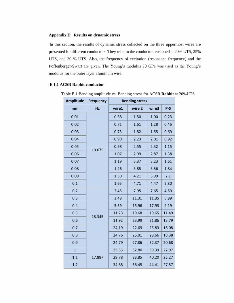
Appendix E: Results on dynamic stress
In this section, the results of dynamic stress collected on the three uppermost wires are
presented for different conductors. They refer to the conductor tensioned at 20% UTS, 25%
UTS, and 30 % UTS. Also, the frequency of excitation (resonance frequency) and the
Poffenberger-Swart are given. The Young’s modulus 70 GPa was used as the Young’s
modulus for the outer layer aluminum wire.
E 1.1 ACSR Rabbit conductor
Table E 1 Bending amplitude vs. Bending stress for ACSR Rabbit at 20%UTS
Amplitude Frequency Bending stress (MPa)
mm Hz wire1 wire 2 wire3 P-S
0.01
19.675
0.68 1.50 1.00 0.23
0.02 0.71 1.61 1.28 0.46
0.03 0.73 1.82 1.55 0.69
0.04 0.90 2.23 2.01 0.92
0.05 0.98 2.55 2.32 1.15
0.06 1.07 2.99 2.87 1.38
0.07 1.19 3.37 3.23 1.61
0.08 1.26 3.85 3.56 1.84
0.09 1.50 4.21 3.99 2.1
0.1 1.65 4.71 4.47 2.30
0.2
18.345
2.45 7.95 7.65 4.59
0.3 3.48 11.31 11.35 6.89
0.4 5.39 15.96 17.93 9.19
0.5 11.23 19.68 19.65 11.49
0.6 11.92 23.99 21.86 13.79
0.7 24.19 22.69 25.83 16.08
0.8 24.76 25.01 28.66 18.38
0.9 24.79 27.86 32.37 20.68
1
17.887
25.33 32.80 39.39 22.97
1.1 29.78 33.85 40.20 25.27
1.2 34.68 36.45 44.41 27.57

Table E.2: Bending amplitude vs. Bending stress for ACSR Rabbit 25%UTS
Amplitude Frequency Bending Stress (MPa)
mm Hz wire 1 wire2 wire3 P-S
0.01
20.4
0.68 1.51 1.20 0.24
0.02 0.78 1.83 1.52 0.48
0.03 0.86 2.27 2.07 0.72
0.04 1.09 2.85 2.66 0.96
0.05 1.16 3.44 3.32 1.20
0.06 1.33 3.83 3.62 1.44
0.07
19.907
1.78 4.71 4.65 1.69
0.08 1.68 4.78 4.67 1.92
0.09 1.99 5.19 4.97 2.17
0.1
18.036
2.19 6.14 5.95 2.41
0.2 3.51 10.02 10.38 4.81
0.3 4.64 14.46 15.08 7.22
0.4 5.82 18.460 19.80 9.63
0.5 21.12 22.74 24.70 12.03
0.6 22.13 26.12 28.36 14.44
0.7 22.57 29.17 32.02 16.84
0.8 31.77 32.31 37.73 19.25
0.9 33.56 35.76 42.62 21.66
1 37.58 39.23 46.59 24.06
1.1 51.51 48.88 47.19 26.47
1.2 52.80 52.30 49.66 28.87

Table E.3. Bending amplitude vs. Bending stress for ACSR Rabbit at 30%UTS
Amplitude Frequency Bending Stress (MPa)
mm Hz wire 1 wire2 wire3 P-S
0.01
20.798
1.01 1.89 1.07 0.25
0.02 1.26 2.61 1.74 0.50
0.03 1.40 3.20 2.35 0.75
0.04 1.71 4.11 3.20 1.00
0.05 1.84 4.61 3.81 1.25
0.06 1.98 5.20 4.56 1.50
0.07 2.1 5.79 5.22 1.75
0.08 2.11 5.98 5.49 2.01
0.09 2.27 6.43 5.92 2.26
0.1 2.51 7.07 6.49 2.51
0.2
20.05
4.11 11.44 6.65 5.01
0.3 5.01 13.95 6.81 7.52
0.4 7.71 17.77 7.84 10.02
0.5 10.95 21.84 9.76 12.53
0.6 11.70 25.92 11.24 15.04
0.7 28.64 30.75 31.05 17.54
0.8
19.543
31.75 34.073 35.52 20.05
0.9 34.98 36.89 39.18 22.55
1 42.78 44.86 47.23 25.06
1.1 48.69 50.35 52.48 27.57
1.2 53.16 53.93 56.01 30.07
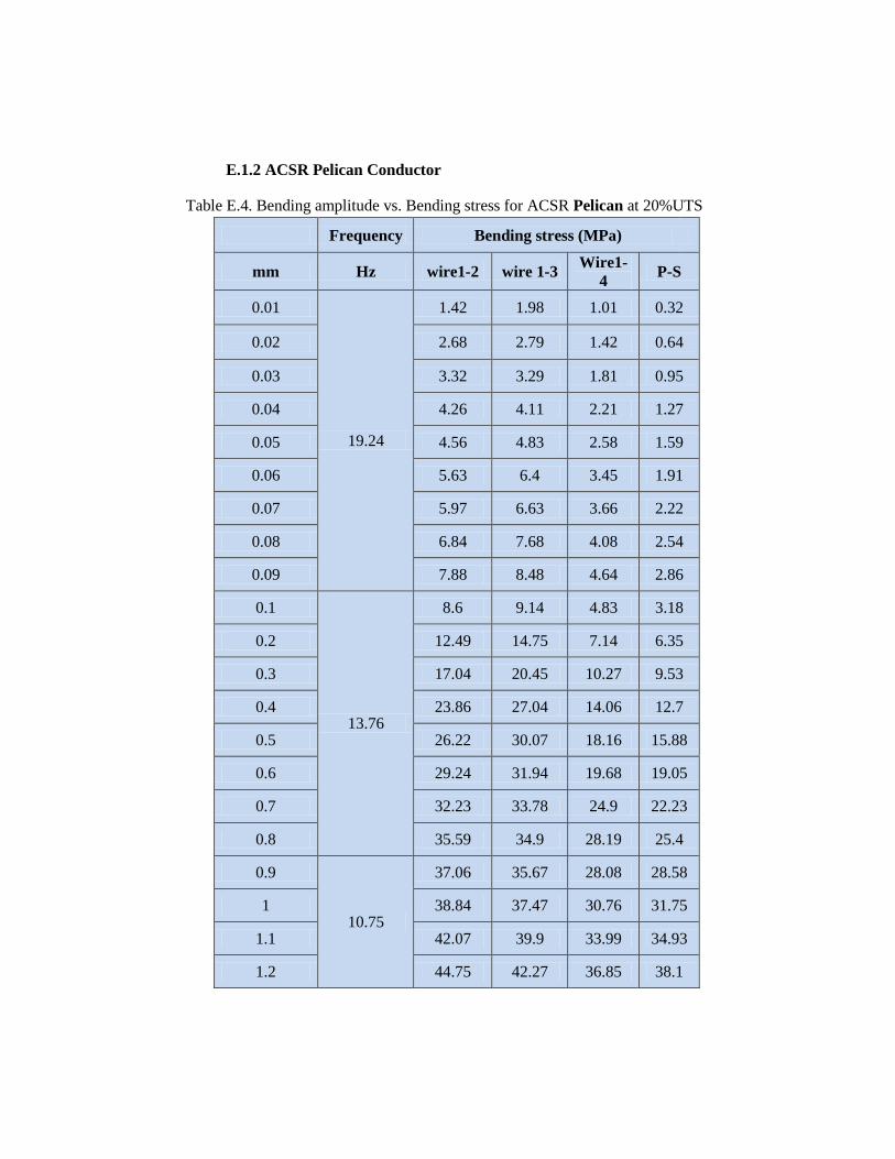
E.1.2 ACSR Pelican Conductor
Table E.4. Bending amplitude vs. Bending stress for ACSR Pelican at 20%UTS
Frequency Bending stress (MPa)
mm Hz wire1-2 wire 1-3 Wire1-
4 P-S
0.01
19.24
1.42 1.98 1.01 0.32
0.02 2.68 2.79 1.42 0.64
0.03 3.32 3.29 1.81 0.95
0.04 4.26 4.11 2.21 1.27
0.05 4.56 4.83 2.58 1.59
0.06 5.63 6.4 3.45 1.91
0.07 5.97 6.63 3.66 2.22
0.08 6.84 7.68 4.08 2.54
0.09 7.88 8.48 4.64 2.86
0.1
13.76
8.6 9.14 4.83 3.18
0.2 12.49 14.75 7.14 6.35
0.3 17.04 20.45 10.27 9.53
0.4 23.86 27.04 14.06 12.7
0.5 26.22 30.07 18.16 15.88
0.6 29.24 31.94 19.68 19.05
0.7 32.23 33.78 24.9 22.23
0.8 35.59 34.9 28.19 25.4
0.9
10.75
37.06 35.67 28.08 28.58
1 38.84 37.47 30.76 31.75
1.1 42.07 39.9 33.99 34.93
1.2 44.75 42.27 36.85 38.1

Table E.5. Bending amplitude vs. Bending stress for ACSR Pelican at 25%UTS
Amplitude Frequency Bending stress (MPa)
mm Hz wire1-2 wire 1-3 Wire1-4 P-S
0.01
19.7
1.41 1.43 0.94 0.335
0.02 2.68 2.79 1.42 0.67
0.03 3.32 3.29 1.81 1.01
0.04 4.26 4.11 2.21 1.34
0.05 4.56 4.83 2.58 1.68
0.06 5.63 6.4 3.45 2.01
0.07 5.97 6.63 3.66 2.35
0.08 6.84 7.66 4.08 2.69
0.09 7.87 8.48 4.64 3.02
0.1
13.894
8.6 9.14 4.83 3.36
0.2 12.46 14.75 7.14 6.71
0.3 17.04 20.49 10.27 10.07
0.4 23.86 27.04 14.06 13.42
0.5 26.22 30.07 18.16 16.77
0.6 29.24 31.93 19.68 20.13
0.7 32.23 33.78 24.9 23.49
0.8
10.564
35.59 34.9 28.19 26.84
0.9 37.06 35.67 28.08 30.2
1 41.16 37.76 32.67 33.55
1.1 42.04 38.97 35.25 36.91
1.2 42.2 40.38 37.1 40.26

Table E.6. Bending amplitude vs. Bending stress for ACSR Pelican at 30%UTS
Amplitude Frequency Bending stress (MPa)
mm Hz wire1 wire 2 wire3 P-S
0.01
16.5
2.41 2.53 1.03 0.35
0.02 3.08 3.16 1.52 0.71
0.03 3.88 3.73 2.01 1.06
0.04 4.58 4.51 2.58 1.41
0.05 5.39 5.09 3.013 1.76
0.06 6.31 5.77 3.47 2.11
0.07 7.21 6.49 3.97 2.47
0.08 7.52 6.97 4.19 2.82
0.09
14.543
8.74 7.66 4.73 3.168
0.1 9.45 8.25 5.26 3.52
0.2 12.75 8.84 7.18 7.04
0.3 18.33 12.69 12.22 10.56
0.4 22.45 17.39 13.37 14.08
0.5 25.75 20.05 14.83 17.6
0.6 30.23 25.14 16.08 21.12
0.7
11.235
34.11 28.44 18.8 24.64
0.8 37.86 31.77 21.96 28.16
0.9 40.97 34.19 31.47 31.68
1 42.88 38.85 35.34 35.2
1.1 45.16 40.68 37.35 38.72
1.2 47.38 42.49 39.98 42.24

E.1.3. ACSR Tern conductor
Table E.7. Bending Amplitude vs. Bending stress for ACSR Tern 20%UTS
Amplitude Frequency Bending stress (MPa)
mm Hz wire1-2 wire 1-3 Wire1-4 P-S
0.01
19.373
0.908747 0.981094 1.083206 0.3232
0.02 1.314018 1.668125 1.571976 0.6464
0.03 1.781696 2.415237 2.130345 0.9696
0.04 2.259378 3.043027 2.620454 1.2928
0.05 2.58167 3.615601 3.060627 1.616
0.06 3.07695 4.298454 3.586485 1.9392
0.07 3.476662 4.857544 4.091761 2.2624
0.08 3.892341 5.434468 4.561642 2.5856
0.09 4.271398 5.951305 4.983875 2.9088
0.1
17.938
4.703175 6.435319 5.484302 3.232
0.2 8.998269 11.056 9.998605 6.464
0.3 12.81294 15.64571 13.82461 9.696
0.4 17.10406 17.8697 15.38976 12.928
0.5 21.20427 20.09504 20.25043 16.16
0.6 22.55762 23.76453 25.87853 19.392
0.7 23.91851 26.1303 26.74751 22.624
0.8
13.633
24.75582 28.01391 27.58344 25.856
0.9 26.3254 31.41104 29.78935 29.088
1 29.654 35.2285 32.765 32.32

Table E.8. Bending Amplitude vs. Bending stress for ACSR Tern at 25%UTS
Amplitude Frequency Bending stress (MPa)
mm Hz wire1-4 wire 1-5 Wire1-6 P-S
0.01
19.019
0.981094 0.684309 1.254012 0.3272
0.02 1.686687 1.568467 1.633403 0.6544
0.03 2.324868 2.172575 2.382268 0.9816
0.04 3.0317 2.721605 2.963955 1.3088
0.05 3.689297 3.371256 3.404013 1.636
0.06 4.060153 3.873368 3.829683 1.9632
0.07 4.921906 4.516635 4.448335 2.2904
0.08 5.504103 5.16441 4.980745 2.6176
0.09 6.122636 5.807723 5.253766 2.9448
0.1
17.342
6.435319 5.07609 6.119529 3.272
0.2 11.056 11.21362 10.66461 6.544
0.3 15.64571 15.55626 15.82723 9.816
0.4 17.8697 19.43104 21.12866 13.088
0.5 20.09504 24.1832 25.3997 16.36
0.6 23.76453 29.2297 29.32599 19.632
0.7 26.1303 33.88063 33.84447 22.904
0.8
13.876
28.01391 37.27659 36.79731 26.176
0.9 31.41104 40.8545 39.01651 29.448
1 35.2285 42.83232 40.1586 32.72

Table E.9. Bending amplitude vs. Bending stress For ACSR Tern at 30%UTS
Amplitude Frequency Bending stress (MPa)
mm Hz wire1-4 wire 1-5 Wire1-6 P-S
0.01
19.253
1.686182 1.292363 2.508025 0.343
0.1 5.693985 5.72691 6.119529 3.43
0.02 2.071255 2.656151 1.633403 0.686
0.03 2.75662 3.653501 2.382268 1.029
0.04 3.590345 4.403012 2.963955 1.372
0.05 4.191897 4.995076 3.404013 1.715
0.06 4.331525 5.274014 3.829683 2.058
0.07 4.812239 5.744612 4.448335 2.401
0.08 5.104185 5.964056 4.980745 2.744
0.09
17.938
5.311789 6.235452 5.253766 3.087
0.2 10.43021 11.12648 10.66461 6.86
0.3 15.09076 16.63439 15.82723 10.29
0.4 18.50116 23.27032 21.12866 13.72
0.5 23.78427 28.59327 25.3997 17.15
0.6 27.85864 32.42979 29.32599 20.58
0.7 33.27398 36.15652 33.84447 24.01
0.8
15.242
36.41502 38.14903 36.79731 27.44
0.9 38.765 39.01651 38.8999 30.87
1 40.1235 41.1586 40.2336 34.3

E1.4 ACSR Bersfort conductor
Table E.10: Bending amplitude vs. Bending stress for Bersfort 20 %UTS
Amplitude Frequency Bending stress (MPa)
mm Hz wire1-4 wire 1-5 wire 1-6 P-S
0.01
22.582
0.892591 1.047984 0.630622 0.343
0.02 1.245433 1.623694 0.974568 0.686
0.03 1.741145 2.270633 1.362426 1.029
0.04 1.989651 2.79779 1.652828 1.372
0.05 2.563813 3.500517 2.060616 1.715
0.06 2.633127 4.042436 2.136198 2.058
0.07 3.175368 4.58307 2.294606 2.401
0.08 3.713037 5.00654 2.916923 2.744
0.09 4.066397 5.410348 3.192504 3.087
0.1 4.267024 5.784436 3.460512 3.43
0.2
19.668
7.958936 9.144328 5.974969 6.86
0.3 9.717359 11.68051 7.485904 10.29
0.4 13.15374 15.18074 7.85207 13.72
0.5 15.18811 17.42129 9.716097 17.15
0.6
17.43
18.81815 19.45157 11.93372 20.58
0.7 20.34222 24.51679 14.77861 24.01
0.8 23.42746 28.7539 19.3658 27.44

Table E. 11: Bending amplitude vs. Bending stress for ACSR Bersfort 25 %UTS
Amplitude Frequency Bending stress (MPa)
mm Hz wire1-4 wire 1-5 wire 1-6 P-S
0.01
23.619
1.007272 0.881305 0.796175 0.361
0.02 1.485323 1.828154 1.015107 0.722
0.03 2.118971 2.705148 1.572424 1.083
0.04 2.505617 3.026193 1.710355 1.444
0.05 2.980746 4.113223 2.283887 1.805
0.06
21.990
3.388813 4.388551 2.642048 2.166
0.07 3.560299 4.960062 2.964875 2.527
0.08 4.474748 5.644342 3.3185 2.888
0.09 4.884755 6.212722 3.61839 3.249
0.1
19.547
5.295049 7.274132 4.092582 3.61
0.2 10.40566 12.75579 7.68607 7.22
0.3 14.33998 15.57262 10.57847 10.83
0.4 17.84844 19.64262 12.67019 14.44
0.5
17.918
20.84281 21.28854 15.22485 18.05
0.6 25.12727 25.87841 20.05976 21.66
0.7 27.909 28.8715 21.8855 25.27
0.8 28.9716 30.303 24.206 28.88

Table E 12: Bending amplitude vs. Bending stress for ACSR Bersfort at 30 %UTS
Amplitude Frequency Bending stress (MPa)
mm Hz wire1-4 wire 1-5 wire 1-6 P-S
0.01
23.197
1.159793 2.492723 1.083954 0.381
0.02 1.524289 3.165234 1.108132 0.762
0.03 1.865556 3.209415 1.51771 1.143
0.04 2.470392 4.471789 1.971379 1.524
0.05 2.831859 4.861946 2.46738 1.905
0.06 3.151338 5.019016 2.84089 2.286
0.07
21.412
3.584823 5.565041 3.137443 2.667
0.08 3.658642 5.901427 3.337074 3.048
0.09 3.881815 6.252484 3.514938 3.429
0.1 4.450131 6.559146 3.934529 3.81
0.2 7.846358 10.43627 7.6615 7.62
0.3 11.92515 14.71207 11.23815 11.43
0.4 16.58701 18.55242 14.3185 15.24
0.5
19.628
19.44689 23.51716 17.95627 19.05
0.6 23.28642 25.66559 19.45909 22.86
0.7 24.94707 27.55418 20.08909 26.67
0.8 27.00233 30.73978 23.7889 30.48

Appendix F: Evaluation Lifetime and Vibration severity (CIGRE)
The flow chart below gives an overview of different steps in the evaluation of the conductor
lifetime and vibration severity.
Figure F.1. Flow chart giving the step in the evaluation of the vibration severity (CIGRE)
Data from
the Vibration
Recorder
Bending
amplitude
P-S or lab
test
Miner’s
rule
Bending
stress/Strain Lifetime
Utility limits
EPRI IEEE CIGRE
limits
EPRI limits
Evaluation of Vibration Severity

Appendix G: Copy of Conference Publication
http://www.ndt.net/article/wcndt2012/papers/118_Kubelwa.pdf
