the redshifts in relativity · 2016-01-25 · mathematical model for expanding universe that had a...

European Journal of Physics Education Vol. 2 No. 2 ISSN 1309 7202 Singh Singh Hareet

24

The Redshifts in Relativity

Satya Pal Singh Department of Applied Sciences, MMM Eng. College

Gorakhpur-273010, UP, India Email: [email protected]

Apoorva Singh

Department of Mechanical Eng, MMM Eng. College Gorakhpur-273010, UP, India

Prabhav Hareet Department of Electrical Eng, MMM Eng. College

Gorakhpur-273010, UP, India

Abstract

The progress of modern cosmology took off in 1917 when A. Einstein published his paper on general theory of relativity extending his work of special theory of relativity (1905). In 1922 Alexander Friedmann constructed a mathematical model for expanding Universe that had a big bang in remote past. The experimental evidences could come in 1929 by the pioneering work on nebular red shifts by Edwin Hubble and Milton H red shift for light also comes as a deduction of special theory of relativity which provides a fundamental formalism for observational astronomy. It can also be deduced from cosmological red shift arising from the curvature of space time warp of the Universe depending on the evolution model opted for the Universe. The gravitational red shift comes as a consequence of the principle of equivalence in presence of weak gravitational field which expresses the identity of the gravitational and inertial mass. The gravitation itself is a manifestation of curvature in space time. Massive objects show noticeable bending of light near it which explains well the apparent images formation when added with the gravitational fall of the photons towards the object. Special and general theory of relativity can be realized as the best mathematical narrations of the cosmic dance. This paper highlights the experimental evidences in favor of relativity and their applications in cosmology which could be possible with the invention of ultra high precision instruments in the latter half of the last century. Keywords: Relativity, redshift, general relativity, gravitational field. Introduction

gravitational and cosmological red shift. Space-time warp, gravitation and the principle of equivalence are also discussed to establish their importance in connection with modern cosmology. The special theory of relativity deals with the relation, which exist between physical entities as they appear to different observers who are in motion. The general theory of relativity describes the equivalence of observations in weak gravitational field and observation made in an accelerating frame of reference. According to special theory of relativity there exist infinite numbers of inertial frames of reference which are equivalent. By the virtue it is impossible to decide between two inertial frames of reference that which one is moving and which one is at rest. All dynamical laws are


25

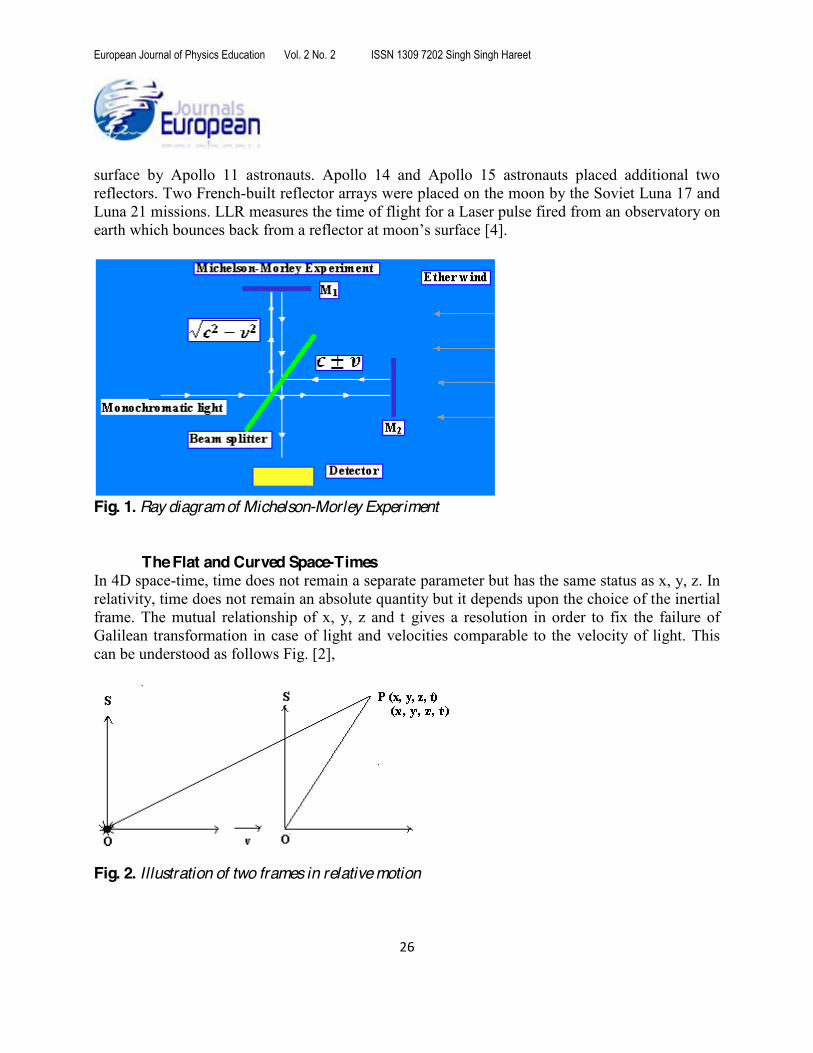
identical in inertial frames of reference and it is impossible to decide by any dynamical experiment which can enable us to detect absolute uniform motion. The prevailing idea before the beginning of the 20th century was that there exists one absolute frame of reference filled with some hypothetical medium ether with nearly zero density in which the law of optics and electromagnetic field assume a particularly simple form. In this field the most important experiment was performed by Michelson Morley .They found that no relative motion between ether and earth exist within their experimental accuracy of 0.04 fringe shift Fig. [1]. After Michelson-Morley there have been more than 400 experiments for testing the ether hypothesis or in other words the isotropic nature of space time using improved and sophisticated techniques [1] [2]. For two inertial frames moving along X direction the metric transforms as-

to ).

Here, ds represent the geodesic. The special theory of relativity corresponds to g0=g1=g2=1. Joos version of Michelson-Morley experiment showed that g2/g1- -11. Improved laser test using He- -Perot interferometer gave an orders of magnitude

-15 corresponding to the value of g2/g1- -15. The Michelson-Morley experiment and its modern improvements told us that the speed of light is isotropic in all inertial frames as predicted by the principle of relativity. But principle of relativity says more than this by assigning a constant numerical value of this isotropic speed of light as c = 2.99 8 meter/sec. This verification was carried out by R. J. Kennedy and E. M. Thorndike about 50 years after Michelson and Morley. Kennedy and Thorndike also used the earth as a moving frame of reference. They also concluded with negative results as- there is no significant variation in speed of light in two different inertial frames attached with the earth (< 2.0 meter/sec in two frames moving with relative velocity of 60 Km/sec attached with the earth. The orbital velocity of earth is 30 Km/sec) [3]. In their experiment they have used the interferometer base itself as the standard length. The standard of time was provided by the characteristic vibration period associated with a particular green spectral line of a mercury atom. ory of relativity GTR could start its empirical success in 1915 by

confirmed the doubling of the deflection angles predicted by general relativity as compared to Newtonian and equivalence principle arguments. The general theory of relativity has been verified at higher accuracies since then [4]. Microwave ranging to the Viking landers on Mars yielded a ~ 0.2% accuracy via the Shapiro time delay. Spacecrafts and planetary radar observations reached an accuracy of ~0.15%. Lunar Laser ranging (LLR) has provided verification of general relativity improving the accuracy to ~0.05% via precision measurements of the lunar orbit. The astronomical observations of the deflections of quasar positions with respect to the Sun performed with very long base line interferometer (VLBI) proved the general relativity with an accuracy of ~0.045%. The time delay experiment with the Cassini spacecraft at a solar conjecture has tested gravity with remarkable accuracy of ~0.0023%. Lunar Laser Ranging (LLR) has a history dating back to the placement of a retro reflector


26

surface by Apollo 11 astronauts. Apollo 14 and Apollo 15 astronauts placed additional two reflectors. Two French-built reflector arrays were placed on the moon by the Soviet Luna 17 and Luna 21 missions. LLR measures the time of flight for a Laser pulse fired from an observatory on

[4].

Fig. 1. Ray diagram of Michelson-Morley Experiment

The Flat and Curved Space-Times

In 4D space-time, time does not remain a separate parameter but has the same status as x, y, z. In relativity, time does not remain an absolute quantity but it depends upon the choice of the inertial frame. The mutual relationship of x, y, z and t gives a resolution in order to fix the failure of Galilean transformation in case of light and velocities comparable to the velocity of light. This can be understood as follows Fig. [2],

Fig. 2. Illustration of two frames in relative motion


27

Let t=t =0, both the co-ordinate frames S and S ther. The same starts moving in

e light ray reach to point P in space whose co-ordinates

In this case,

(1) (2)

Substituting Galilean transformation equations gives, (3)

(4)

The lower equation has two terms extra as v2 t2-2 x v t in its left side in comparison to the

earlier equation. This is a contradictory case. It can work as a hint that the time and space are not as separate entities as were thought. The electromagnetic theory was recognized long before relativistic invariance but his equations had similar inconsistencies in his contemporary world. One could conclude that the Galilean transformation fails for relativistic classical mechanics and for electrodynamics as well. In other words it also hinted that there were some flaws in the absolute concept of space and time. Hertz demonstrated electromagnetic waves in 1887 generated by oscillating currents in a macroscopic electric circuit. The frequencies he generated were around 109 Hz with a corresponding wavelength of 30 cm. Hertz experiments were significant turning point [5]. Though, it would not look like a concrete statement until one derives the Lorentz transformation in which it is essentially assumed to successfully remove the above mentioned contradictions of Galilean transformation in relativistic limits. Lorentz worked for the transformations named after him on a completely adhoc basis which did not represent the physical quantities specifically as time and was supposed to be true in general. It is the Lorentz

which satisfy the above two equations simultaneou - 2)-1/2

time dilation in motion. Space and time are united into a single geometric entity. The laws of nature can be expressed as the property of covariance of any physical process with respect to transformations involving the four dimensional space time co-ordinates. Thus the multiplicity of space-time representations of events is only possible with invariant physical quantities in order to permit the laws of nature to be true as Poincare had first suggested.


28

The Metric Form or Metric Tensor of Space- Time Warp The flat and curved space time can be understood by representing it in simple metric form [6]. The distinction between flat and curved space Fig. [3] is that for a flat two dimensional space, it is possible to find a co-ordinate system in which metric form is everywhere.

(5)

With the coefficients of dx2 and dy2 being 1. This implies arbitrarily large displacements or distances. Opposite to above, no such co-ordinate system can be found for a curved space (e.g. on the surface of a sphere). Similar results hold for higher- dimensional spaces. As for example a three dimensional space is flat if and only if co-ordinates x, y, z can be found such that the metric form there is

(6)

The above relation can be locally true on a curved surface caused by a massive body. It is convenient here to introduce a general metric tensor notation that is applied to all the spaces in higher dimensions specially the space - time we have considered. We can locate a point (x, y, z) on the surface of the sphere as follows:

Which, satisfies the surface of a sphere which is non Euclidean and given by,


29

Fig. 3. A) Positive curvature surfaces and B) Negative curvature surfaces; the left lower photograph shows a possible world line depicting the events of signal delays passing through celestial objects for which gik ik being constant does not ensure that we are dealing with a non Euclidean space as one can learn from the following transformation

; again here gik are functions of

I llustrations of Space-Time

In our solar system, the nine planets (now 8) move in their orbit around sun. Ireference, the sun is at rest while the planets circle around it describing a helix in space-time. The

surfaces of instantaneity trace out a circle around the sun. Here flat space-time is considered and curvature produced in space time due to the solar mass is not taken into account to simplify the picture [7].


30

Fig. 4. Shows different time snap shots of our planet circling around the Sun

Fig. 5A. Men moving up with an elevator

Here two snap shots Fig. 5A and Fig. 5B of customers going to upper floor using escalator in a shopping mall are taken at two different instants. We can consider the positions of the group of men as two separate events occurring at two different time slots and at same position coordinates. One can imagine in space-time the space co-ordinates are moving upwards


31

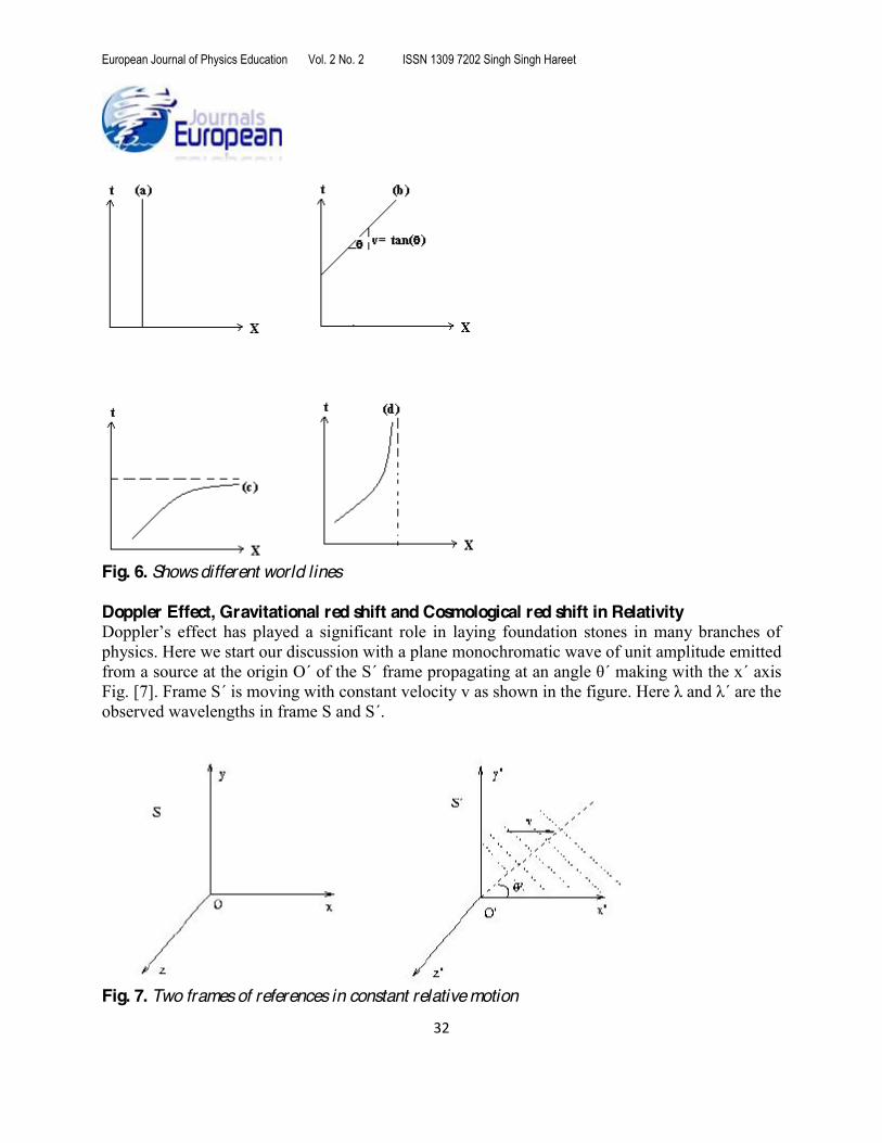
Fig. 5B. Men moving up with an elevator or escalating on the ruler of time. The pictures A and B give us an analogous understanding of the events in four dimensional space and time. Though, the particle moves in four-dimensional space- time, but it is much easier to draw two-dimensional diagrams. The three spatial co-ordinates x, y, z are represented by one single co-ordinate x, each particle corresponds to a line, called world line in space- time graph. For example four different world lines are shown for different type of motion [8] Fig. [6]. It is important to note here that not all lines in space- time are possible world lines. For example, if a line reaches a maximum time and then slopes down again; it does not represent a possible world line of a massive body because time would start running backwards along such a world line where its slope is downwards.


32

Fig. 6. Shows different world lines Doppler Effect, Gravitational red shift and Cosmological red shift in Relativity

physics. Here we start our discussion with a plane monochromatic wave of unit amplitude emitted of the S frame pro axis

Fig. [7]. Frame S is moving with constant velocity v as shown in the figure.

Fig. 7. Two frames of references in constant relative motion


33

(7)

(8)

(9)

(10)

(11)

(12)

(13)

(14)

The recessional redshift of light has helped scientists to directly measure the velocities of

the distant moving celestial objects. The most significant direct light geared the contemporary scientist of Edwin Hubble and his predecessors to establish the concept of the expanding Universe which lead to the idea of hot big-bang model of the Universe in decade of 1940. It could be realized that the Universe originated form a singular infinitesimally small point in remote past and is ever expanding after an explosion. As for example red shift for 3C273 - 0 0=0.158 & 3C48; z=0.367 which gives a direct measure of their recessional speed.

The Equivalence Principle and the Gravitational Redshift According to the equivalence principle, the events taking place in an accelerated laboratory cannot be distinguished from those which take place in gravitational field. How can one distinguish between an accelerated frame and a true gravitational field? Gravitational field is real and cannot be eliminated at all places by simply choosing a non-inertial or say accelerated frame due to non-uniformity of the actual gravitational field. Gravitational field vanishes at a large distance from the source, where as an accelerated frame can eliminate the gravitational field only locally. Thus frames when falling freely must have acceleration due to gravity valid only in the small region if we consider two freely falling particles wide apart on the surface of the earth and hence their accelerations cannot be paralleled Fig. [8].


34

Fig. 8. Freely falling lifts at two different places in earths weak gravity

If one of these two bodies is placed in a freely falling elevator that will cancel the effect of gravitational force to an observer in that lift. But second will seem to approach towards the first one and with some definite acceleration.

Gravitational Redshift When light propagates against a gravitational field, it loses energy progressively. This is manifested as an increase in its wavelength. This phenomenon is known as gravitational red shift [9] [10] [11] [12].

Fig. 9. Shows two positions of a freely falling lift

According -gravitational experiment can distinguish a freely falling non-rotating system (local inertial system) for a uniformly moving system in the absence of gravitational field. An immediate

blue shift Fig. [9]. Let us consider an elevator cabin in a static gravitational field of strength g. Suppose the cables holding the elevator cabin is broken at


35

emitted from its ceiling towards the floor. An observer B at rest in the shaft reaches at the same height as point A of the floor when the photons reach there. B moves with a velocity v =gt relative to A. therefore B sees the light Doppler shifted to the blue end by an amount-

----(15)

Where is the difference in the Newtonian potential between the receiver and the emitter at rest at two different heights. The most precise result so for was achieved with a rocket experiment that brought a hydrogen-10-4. Gravitational red shift effects are routinely taken into account to correct clocks used in Global Positioning System (GPS).

(15)

(16)

(17)

Fig. 10. A pictorial representation (not up to any real scale) of apparent shift in wavelength near a massive object T2 T1 =T0*(U2 U1) / c2. If U2 is the potential on the Sun and U1 is the potential on the earth, then we have U2 > U1. (U2 U1) / c2 . Thus the wavelengths of spectral line originated on the Sun must be displaced relative to the corresponding lines produced on the earth by two parts in a million toward the red end of the spectrum.

Theoretical calculations by mathematician and astronomer Herman Bondi tells us that

any astronomical body held in equilibrium under forces of gravity and outward pressure of gas or radiation can have a maximum red shift of no more than 0.7 from its surface. But the observational anomalies that require explanation are much higher as 5-6. Fred Hoyle and Willy Fowler explained that for a compact massive object the red shift may be much higher if the light


36

has left form its interior and escape without any significant absorption but these are still more speculative way of explaining the observed phenomena to model for the observed events with the help of known theories.

Example Experiment of Pound and Rebka:

Pound and Rebka (1960) performed the first experiment to measure the small gravitational red shiftkeV. The emitter and the observer were placed at the bottom and at the top of a tower 22.6 m

a small suitable velocity was imparted to emitter towards the absorber. This motion would generate the appropriate blue- shift by Doppler effect and cancel the original gravitational red shift creating a situation for

-rays. Evidence of Warped Space time:

Mass curves the space and space tells mass how to move. The massive object curves the space time warp [13]. An analogous example is the case of rubber stretch which bulges out when a heavy ball is placed over this Fig. [11]. Any moving pellet when reaches in this sheet it will start whirling around the bigger ball. The massive object in cosmology are stars, galaxies, cluster of stars and galaxies, massive dwarf stars as white dwarf stars, neutron stars, black holes etc. The bending of space time warp is more pronouncedly observed near compact and composite stars, pulsars and quasars etc which can cause many image formations of stars because of bending of light coming from the farther backyards of these. Black holes are the cold remnants of former stars. This phenomenon is called gravitational lensing Fig. [12]. and Fig. [13] show photographs of one such gravitational lensing cluster Cl0024+16 taken by Hubble Space Telescope. The black holes one of the dwarf star are so densely packed that not even light can escape out of its gravitation. When giant stars reach to their final stages of lives they detonate as supernova explosions. Such an explosion scatters most of the stars matter into large voids of the space but can leave behind a large which fusion process no longer takes place and the gravitational collapse is balanced by the electron and neutron degeneracy respectively known as white dwarf star and neutron star. If the mass of the proto star is less than the critical Chandrasekhar limit of 1.44 solar masses, electrons librated from the ionized He+ experience out

balance the gravitational fall inwards. When the mass exceeds the Chandrasekhar limit but is less than 2-3 solar mass, the electrons and protons gain sufficient energy to combine together to form neutron and in that case the balance is achieved by neutron degeneracy [14]. The black hole are formed when the mass of the dead star is more than 3 time the solar mass. The stars more massive than 3 time the solar mass ends their lives as black holes with extraordinary limit of curvature in their space time warp so that even light cannot escape these and either can keep on whirling for ever or can be absorbed.


37

Fig. 11. Shows space-time warp near a massive celestial object

Fig. 12. Quasar Images are formed because of gravitational lensing


38

Fig.13. A gravitational lensing cluster Cl0024+16 are shown in the photograph taken by Hubble Space Telescope

The cosmological Redshift

The most general line element satisfying cosmological principle given by H P Robertson and A G Walker can be written as follows [15]-

(18)

Each galaxy can be allocated a constant set of coordinate (r, , ) in cosmological rest frame. Let us consider a galaxy at G1 at (r1 1, 1) emitting light rays towards us. Let t0 be present epoch of observation. One needs to know the time when light had left from G1. From the symmetry of a space time one can guess that a null geodesic from r=0 to r=r1 will ma 1, = 1 all along the null geodesics. Thus for the Robertson-Walker line, we get

(19)


39

Since r decreases as t increases along null geodesic, we should take the negative sign in the above relation. Suppose the null geodesic left G1 at time t1 which gives-

(20)

Suppose the wave crests are emitted at t1 and t1 1 and received at t0 and t0 0 respectively. (21)

If S (t) is a slowly varying function so that it effectively remains unchanged over the small 0 1, we get from subtraction

(22)

(23)

1 is measured by an observer at rest in the galaxy G1 2 is measured by an observer at rest in our galaxy. This effect arises from the passage of light through a non-Euclidean space

red shift. be deduced from this. Cosmological redshift comes as a consequence of space-time warp in 4 dimensional Einstein-Minkowski world where time is kept at equal footing with usual spatial co-ordiantes as x, y, z to define the real fabric of the space. Of course then one can realize that

The Expanding Universe Many observations have been reported from 1912-1930 about different galaxies but a conclusive remark about the expanding Universe could come because of Edwin Hubble in 1929. Hubble observed every fifth brightest stars of different galaxies and shown that the velocities of different galaxies corresponding to observed red shift were found to be proportional to their distances Fig. [14]. Main sequence of equally bright stars allows measuring and comparing their relative distances. He observed about more than 20 galaxies. Others have made observations but very small cluster of galaxies. Hubble also made serious efforts to decide the space-time curvature of the Universe. Hubble also first tried to decide the correct model of the Universe by counting galaxies in given volume of the universe. If one draws a sphere in a closed space, its volume will be less than that in Euclidian flat space. So number of galaxies can be predicted to be less. But such variations become noticeable only beyond 3000 million light years. Since the number of galaxies to be counted runs to millions and the astrophysical objects become fainter to resolve accurately, Hutheoretician R C Tolman. (Shifted)


40

Name of the galaxy Distance in light years Recessional velocities (Red shift)

Virgo 78,000,000 ly 1200 Km/sec Ursa major 1,000,000,000 ly 15,000 Km/sec Coronce Borwlis 1,400,000,000 ly 22,000 Km/sec Bootes 2,500,000,000 ly 39,000 Km/sec Hydra 3,960,000,000 ly 61,000 Km/sec

Table 1. The distance of the galaxies and the observed red shift [16]

= cz = H0 D where H0 constant because of statistical limits and unresolved systematic errors in his observations.

Fig. 14. The velocities of the fifth brightest stars in different constellations vs. their distances

is most popularly known


41

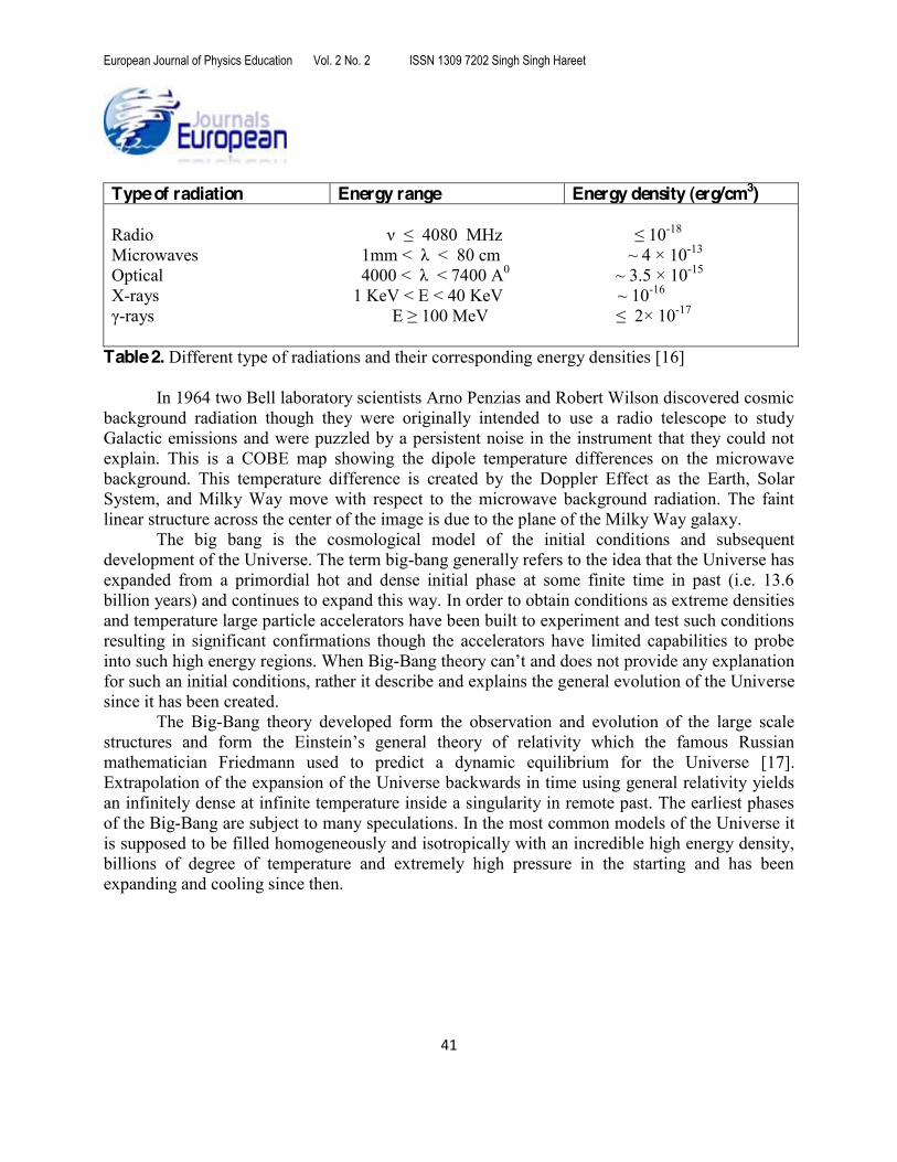
Type of radiation Energy range Energy density (erg/cm3) Radio 80 MHz -18

Microwaves -13 Optical 0 0-15 X-rays 1 KeV < E < 40 KeV ~ 10-16 -rays -17

Table 2. Different type of radiations and their corresponding energy densities [16]

In 1964 two Bell laboratory scientists Arno Penzias and Robert Wilson discovered cosmic

background radiation though they were originally intended to use a radio telescope to study Galactic emissions and were puzzled by a persistent noise in the instrument that they could not explain. This is a COBE map showing the dipole temperature differences on the microwave background. This temperature difference is created by the Doppler Effect as the Earth, Solar System, and Milky Way move with respect to the microwave background radiation. The faint linear structure across the center of the image is due to the plane of the Milky Way galaxy.

The big bang is the cosmological model of the initial conditions and subsequent development of the Universe. The term big-bang generally refers to the idea that the Universe has expanded from a primordial hot and dense initial phase at some finite time in past (i.e. 13.6 billion years) and continues to expand this way. In order to obtain conditions as extreme densities and temperature large particle accelerators have been built to experiment and test such conditions resulting in significant confirmations though the accelerators have limited capabilities to probe into such high energy regions. When Big-for such an initial conditions, rather it describe and explains the general evolution of the Universe since it has been created.

The Big-Bang theory developed form the observation and evolution of the large scale

mathematician Friedmann used to predict a dynamic equilibrium for the Universe [17]. Extrapolation of the expansion of the Universe backwards in time using general relativity yields an infinitely dense at infinite temperature inside a singularity in remote past. The earliest phases of the Big-Bang are subject to many speculations. In the most common models of the Universe it is supposed to be filled homogeneously and isotropically with an incredible high energy density, billions of degree of temperature and extremely high pressure in the starting and has been expanding and cooling since then.


42

Fig. 15. Shows the average distribution of matter and radiation in Universe changing with time; this plot has been obtained using parametric solutions- R = A2 ( 1 2 sin

of the closed Universe model by solving equation no. (28) by programming in Mathematica software.

Fig. 16. Shows the perihelion motion of Mercury around Sun which can be well explained on the

General Theory of Relativity

The Friedmann equation is given by, (24)

The continuity equation can be reduced to (25)

Observational evidence to the date suggests that the Universe is matter dominant and the pressure is negligible when compared the volume and the density. With p=0, one finds that

(26)


43

The Friedmann equation turns out to be- (27)

Here 2

2 0083

G RA (A>0). The subscript zero denotes the present day values of the

H (t) is defined by ( )( ) ( )R tH t R t . Equation (27) reduces to-

(28)

Here k > 0 ( 0 c ), k = 0 ( 0 c ) and k < 0 ( 0 c ) corresponds to closed model,

flat model and open model of the Universe respectively. 2038c

HG .

Since the Universe was smaller in the beginning, one expects both radiation and matter densities to be extremely high. It turns out that the radiation density rises very steeply as compare to matter density when we stretch back in past. The variations in radiation and matter densities are plotted with time on Fig. [15] though not scaled as exponentially increasing and decreasing functions of time with arbitrary parameters. One can realize with the two curves that if volume of the Universe is kept constant then a conversion of radiation into matter will eventually lead to sharp increase in future but that is not so. When the volume of the Universe subsequently obtained from the radius R (t) is used given by the Friedmann model which suggest a changing solution of R (t) with time for the cosmological evolution, the matter density dominates the radiation density but does not shoot up.

In order to obtain conditions as extreme densities and temperature large particle accelerators have been built to experiment and test such conditions resulting in significant confirmations though the accelerators have limited capabilities to probe into such high energy regions. When Big-conditions, rather it describe and explains the general evolution of the Universe since it has been created. The Big-Bang theory developed form the observation and evolution of the large scale

Fig. [16], which the famous Russian mathematician Friedmann used to predict a dynamic equilibrium for the Universe. Extrapolation of the expansion of the Universe backwards in time using general relativity yields an infinitely dense at infinite temperature inside a singularity in remote past. The earliest phases of the Big-Bang are subject to many speculations. In the most common models of the Universe it is supposed to be filled homogeneously and isotropic ally with an incredible high energy density, billions of degree of temperature and extremely high pressure in the starting and has been expanding and cooling since then.


44

Fig. 17. The anisotropic Universe This COBE map Fig. [17] shows fluctuations in the temperature of the microwave background after the effects due to the dipole and the Milky Way have been subtracted out. The level of the fluctuations is less than 20 millionths of a degree. Unlike the dipole temperature variations, these fluctuations are believed to be intrinsic to the CBR itself, resulting from slight gravitational red shifts (blue shifts) due to slight over (under) densities in the early universe at the time of recombination [18] [19]. The discovery of these fluctuations was very significant, for they are due to the small variations in matter density that were present when the CBR decoupled from matter only about 300,000 years after the big bang. These small density variations are the "seeds" that will grow into the galaxies and galaxy clusters in the present universe. The spatial resolution of the COBE satellite was not good enough to observe the fluctuations in enough detail to draw detailed conclusions. A new satellite, the Wilkinson Microwave Anisotropy Probe (named in honor of David Wilkinson) was launched in 2001 to study the CBR in greater detail.

The black body spectrum of the Universe Ground based measurements of the spectrum of radiation coming from all directions of the Universe do not give correct figures as expected for a black body due to atmospheric absorption i.e. vibration modes of water molecules can absorb most of the microwave radiation. The most accurate and exhaustive study was carried out in 1990 by the COBE satellite. The COBE measurements gave a precise Planckian spectrum with a black body temperature of

spherical harmonics as follows [15]-

(29)

The sum over l starts with 1 instead of zero because the zeroth perturbation is isotropic and can be absorbed into T. The l=1 term is the so called dipole-anisotropy term which arises because of the earth motion relative to the rest frame of the MBR. Henceforth this is also not included in the above series. The l=2 term correspond to quadruple mode. The angular power spectrum is specified by quantities Cl defined by-

(30)


45

Which represents the relative strength of the l th harmonic in the overall distribution? The auto covariance function defines the temperature fluctuations comparing over directions separated by

(31)

Here, (32) Stationary fluctuations can be expressed in the form

(33)

The auto covariance function is estimated as (34)

The cosmic covariance of the quantity C ( -

(35)

(cos )lP is the Legendre Polynomial. The Sach- Wolfe effect measures the metric fluctuations near the last scattering surface. Photons coming out of different potential wells producing a change of energy and hence T is given by-

(36)

In addition to this there is a time dilation, so that the photons emerging from a potential well are delayed in relation to surface photons. For Einstein de Sitter Universe S t 2/3 and the fluctuations in T is given by-

(37)

Adding the two effects because the gravitational red shift produces the above time delay (38)

The above fluctuations are cause by gravitational waves and are potentially detectable. Mather and his colleagues used COBE (Cosmic Background Explorer) satellite-based measurements and

noting the fact that the basic physics of big-bang cosmology does not lead to a prediction of its present day temperature. Alpher and Herman came up with a figure or 5K. Gamow the originator himself had a heuristic guess of 7K-15K or even a higher estimate of 50K. Energy density of black body radiation varies as the fourth power of temperature. A guess of 50K is an overestimation by orders of magnitude [20].

There were primordial density fluctuations in matter out of which the galaxies were formed by gravitational collapse. The radiation detected today will contain indications that the earlier distribution of radiation and matter has put a gravitational imprint on the radiation field while radiation was strongly interacting with matter. Dark matter (Fig. [18]) and dark energy:


46

Cosmologist havmatter is 4% (2) the contribution of cold dark matter (CDM) is 23% and (3) the contribution of dark energy is 73% based on their studies of supernova observations and also form the observations of microwave background radiation of the Universe. The rotational speed of neutral hydrogen clouds is plotted against the distance from the center of spiral galaxies remains approximately constant. A large number galaxies show a continuous line. What the astronomers and cosmologist have revealed is that the visible form or matter and energy in the Universe occupy only 4% of total matter-energy of the Universe. The remaining 96% is made of esoteric dark matter and dark energy.

Fig. 18. Distance from the center of the galaxy; the constant rotational velocity indicates for the presence of the dark matter beyond the visible extent of the radius Conclusion

At one place in his autobiographical notes (1949) Einstein wrote about special relativity

development became completely clear to me only in my efforts to represent gravitation in the The principle of relativity was shocking heresy when Einstein first

proposed this in 1905 because it offended the intuition and deeply preconceived ideas of the contemporary world. It has taken a long time to become accustomed and to get apparent acceptance by a large section of scientiby relativity has been unparallel since it was proposed. It is still the best mathematical formulation of the laws of physics. The recent reports of NASA scientists in past 2-3 decades about the accelerating part of the Universe with new ideas of existence of dark energy filling the empty space has got a worldwide attraction among physicists. If one tries to weave this expansion

ion, then the relation can serve as an empirical basis where H0


47

dimensionless parameter [21]of time varying G on its semi-major axis given by but there is no such evidence for local

scale expansion (~1 AU) of the solar system rather such results are realized at larger scales (~20 AU) which in fact will keep on mimicking the ideas such as time varying gravitational concepts and the final and ultimate fabric of the space-time. The possibility of a time variation of the constant of gravitation was first proposed by P. A. M. Dirac in 1938 on the basis of his large number hypothesis [22] and was later developed by Brans and Dicke in the theory of gravitation. Scientist also realize that the uncertainties associated with the precision measurement of the

so many conclusions arising with the data with large systematic and statistical errors and their space time model dependence will keep the speculative thoughts alive and burning. We have tried to study and present an illustrated discussion of key elements of relativity in this paper in the

n context of applications to cosmology. Acknowledgements

Dr. S P Singh expresses his deep and sincere acknowledgements to Inter University Center for Astronomy and Astrophysics (IUCCA), Pune, India for granting for a visit to improve and revise this manuscript and its contents in its present form. Dr. S P Singh expresses his sincere and deep acknowledgements to Prof. Dr. Edwin Turner, Department of Astrophysics, and University of Princeton, USA for sending the reproduction copyright of the gravitational lensing photograph Figure-13 which was taken by him during mid 1990 by HST. The authors also express their thanks to NASA for Figure-13 & 17 which allows for its academic uses for the exploration of science. References

1. Brillet, A., Hall, J.L. (1979). Improved Laser Test of the Isotropy of Space. Phys. Review Letters 42, 549-552.

2. Kenney, Roy J., Thorndike, Edward M. (1932). Experimental Establishment of the Relativity of Time. Phys. Review 42, 400-418.

3. Taylor, Edwin F., Wheelar, John A. (1966). Space Time Phys. W. H. Freeman and Company USA.

4. Williams, James G., Turyshew, Slave G., Boggs, Dale H. (2004). Progress in Lunar Laser Ranging Tests of Relativistic Gravity. Physics Review Letters 93, 261101 (1-4).

5. Purcell, Edward M., Electricity and Magnetism, vol. 2 Tata McGraw-Hill Publishing Company Limited, IInd Edition, New Delhi.

6. Nerlikar, Jayant V., Chapter-2, Introduction to Cosmology, Cambridge University Press.2nd Edition 1993.

7. Hawking, S.W., The theory of everything, (2008). Jaico Publishing House, Edition VIII. 8. Aharoni, J. Lectures on Mechanics (1972) Oxford University Press, US.


48

9. Beiser, Arthur, Concepts of Modern Physics (1995), Edition V, Chapter-1, McGraw-Hill, 10. Singh, S.P. (2009). An Introduction to relativity: Space time and the equivalence

principle. Physics Essays, 22, 3, 314-317. 11. Pound, R. V., Rebka, G. A. (1959). Resonant Absorption of the 14.4-kev Ray from 0.10-

57 Phys. Rev. Letts. 3, 554-556. 12. Landau,L. M.,Lifshitz,E.M.(1998), See chapter 10, Particle in a gravitational field, The

classical theory of fields, A course of theoretical physics, Vol. 2, L. D. Butlerworth-Heinemann, Oxford.

13. Krishnamurthy, Cosmic Panorama, New Age International, New Delhi, India. 14. Ghatak, A., Loknathan, S (1999).p-129, Quantum Mechanics. Macmillan India Limited,

4th Edition 15. Narlikar, J.V. (2010), An Introduction to Relativity, Ist Edition, Cambridge University

Press. 16. Narlikar, J.V. (1993), Introduction to Cosmology,2nd Edition, Cambridge University Press. 17. Foster, J., Nightinagle, J.D. (1995), A Short Course in General Relativity, (p-182),

Springer-Verlag, IInd Edition 18. Ashtekar, A. (2006). Space and Time: From Antiquity to Einstein and Beyond.

Resonance, 9, 4-19. 19. Banerjee, A. (2006). General Theory of Relativity. The Power of Speculative Thought.

Resonance, 11, 45-55. 20. Narlikar, J.V., Bubidge, G. (2008), Facts and Speculations in Cosmology, Cambridge

University Press, Ist Edition. 21. Cattoen, C., Visser, M. (2008). Cosmographic Hubble fits to the supernova data. Physical

Review D, 78, 063501 (1-21). 22. Dirac, P.A.M.(1978), Lecture presented at the School of Physics, University of New

South Wales, Kensington, Sydney, Australia, August 27, 1975. Compiled in- P A M Dirac, Directions in Physics, John Wiley and Sons, 1978, USA

the redshifts in relativity · 2016-01-25 · mathematical model for expanding universe that had a...

Documents