Social & Environmental Benefits of ForestryPhase 2 :

THE RECREATION VALUE OF WOODLANDS

Report to

Forestry CommissionEdinburgh

from

Riccardo Scarpa

Centre for Research in Environmental Appraisal & ManagementUniversity of Newcastle

http://www.newcastle.ac.uk/cream/

March 2003

1/31

Social & Environmental Benefits of ForestryPhase 2:

THE RECREATION VALUE OF WOODLANDS

Riccardo Scarpa

March 2003

1. Introduction

The recreational value of woodlands is a special case of the larger set of values fromoutdoor recreation. As leisure time and population mobility increased in the postworld war II period a large number of applied studies focussed on the social benefitsof outdoor recreation. Initial attempts were predominantly academic exercises, butsoon the benefit estimation methodologies developed by academics were embraced byvarious sectors of society. Nowadays the economic benefits from outdoor recreationare well understood as a result of extensive investigations. The methods to derivethem are routinely taught in environmental valuation modules in the higher educationsystem and are in continuous refinement through the work of researchers in the field.

A perusal of the relevant U.K. and international literature shows that the number ofapplied studies on economic valuation of woodland recreation is second only to waterrecreation studies. In the particular case of the U.K. a large number of applied studiesin forest recreation is available. Many are methodological in nature and are mostlydirected to the academic audience. Many others were carried out to provide answersto specific policy questions as perceived by central and regional government agencies.

The present report covers the specific findings of a study belonging to the second set.The objective is to find the total and marginal recreational value of British forests.The estimates reported are partly based on generic estimates of willingness to pay toaccess forests, as derived from new primary data obtained from contingent valuationsurveys. In part these estimates are also based on the estimation of forest-specificrecreation benefits. The latter were derived from benefit functions estimated from1992 data and updated with the new surveys administered in 2002. More preciselythe methodology employed is known as value transfer from benefit functions. Themain advantage offered by such methodology is that of consistently combining newlycollected primary data with previously collected data, hence building on previousknowledge and thereby achieving a higher level of accuracy than that achievableusing the newly collected data in isolation. More importantly, in the context of thistype of studies, such an approach has the potential to provide large savings in surveyexpenses necessary for basing the valuation entirely on new primary data.

2/31

The report is structured as follows: section 2 outlines the relevant theoretical andempirical issues in recreation benefit estimation, with a particular focus on the task athand and on the literature on estimation of recreational values from benefit functiontransfers; section 3 lays out the methodology and describe the data employed in thisstudy, while section 4 reports the estimation results. Section 5 presents the non-market benefit estimates from recreation in woodlands of the U.K.

2. Estimating woodland recreation values

2.1. Theoretical points of relevance

In estimating benefits from visits to outdoor recreation sites the most frequently usedtheoretical object under investigation is the so-called “compensating variation”, or cv.This is a money measure of the loss of utility individual visitors would suffer fromsite closure. Suppose that the utility level of an individual visitor can be modelled bythe bundle of goods he consumes indicated by the vector z, the income he enjoys m,and ability to access the site, indicated by the scalar x0=1.Implicitly this means that the ith visitor is thought as possessing the right to visitingthe site and hence is entitled to utility level ui(x0

i,zi,mi)=u0i. Under these assumptions

the compensating variation is the amount of money sufficient to return him/her to thelevel of utility u0 when access to the site is precluded because of closure, i.e. x1=0.Implicitly this quantity (cv) is defined as:

ui(x0i,zi,mi) = u0

i = ui(x1i,zi,mi – cv).

Notice that this measure is all-inclusive, and it is net of income substitution and othersubstitution effects. This theoretical measure can be easily derived from statedpreference data, but it is of difficult exact derivation from observed data ontransactions (revealed preference data) (Hausmann, 1981). However, under plausibleconditions it can be adequately approximated by other easy-to-measure quantities,such as consumer surplus measure (cs) (Willig, 1976, 1979). Consumer surplus for site closure is defined as the integral under the inverseMarshallian (uncompensated) demand function between the observed cost of accessand a “choke price” (i.e. a cost of access that would reduce visitation rates to zero).Marshallian demand functions are readily estimated from individual site visitationdata using the cost of travelling to the site as a proxy for individual cost of access, e.g.from travel-cost data. As a consequence the benefit from outdoor recreation in U.K.woodlands has often been estimated from zonal or individual travel cost data (Willis,1991; Willis and Garrod, 1991a, 1992; Bateman et al. 1996). However, although the theoretical discrepancy between exact utility-based benefitmeasures, such as cv, and their approximations from demand functions, such as cs, areshown to be small under the prevalent circumstances of choice for recreationaldecisions, this may well not carry over to large-scale estimation studies, such as theone under consideration. The literature in applied travel cost methodology has

3/31

illustrated a plethora of potential empirical sources of bias in applied travel coststudies (Randall 1994). For example, even the simple choice of including substitutedestinations in the system of demand for travel cost studies can be more difficult thanone may think at first (Caulkins et al. 1986). Household decisions are often not simplyframed around the issue of “what woodland site shall we go and visit?”. Morefrequently they are framed on a broader set of alternatives. For example, around theissue of “what outdoor site shall we go and visit?”, or even a more generic “what shallwe do with this nice day?”. The modelling of the last two decision contexts wouldrequire a much larger set of substitutes than a listing of close-by woodland sites to theone visited. The omission of such a complete set of alternatives from the estimationdemand will bias the derivation of the benefit estimates. This may be unavoidableeven when the researcher employs complex choice-probability travel cost modelsbased on random utility analysis combined with count data (e.g. Hutchinson et al.2002). As a consequence it will introduce a further “empirical” bias, which adds to theexisting theoretical discrepancy between exact and approximate benefit estimates. The above point illustrates the complexity surrounding the decision of what empiricalmeasure to choose for non-market recreation values, such in the case of benefits fromwoodland recreation. The analyst is torn between choosing amongst a number ofapproaches, each providing advantages and disadvantages. For example, travel costmethodologies are often purported as superior as they derive from revealed preferencedata, but as seen above they are not free from theoretical as well as empirical biases.On the other hand stated preference methods, such as contingent valuationapproaches, have the advantage of focussing on the theoretically exact benefitmeasure, but they may display significant sources of empirical bias. Such is the casewhen incentives for hypothetical bias are prevalent, and their effects unadjusted for. A collection of issues complicating the estimation of economic benefits from outdoorrecreation via the travel cost method is reported in Randall (1994). Overall, withcostly data collection, many of these complications can be overcome, but when theobjective is to define a per visit benefit estimate—such as in this case—it wouldappear that uncomplicated stated preference approaches such as the one employedhere, are preferable. In particular, the focus on the benefit value at the woodland gateis conceptually appealing because it is robustly linked to the experience in thewoodland, and unfettered by other issues prior to the decision of access, such as thelength, type and potential multiple-destinations of the journey. 2.2 Objectives and framework of the present investigation In the case of the study at hand the objective is that of providing an estimate of thebenefits from recreational function of woodlands in the U.K., and break it down bycountry and tourist regions. This total estimate must be consistent with the mainmicroeconomic tenets of individual choice and display – in as much as possible –sensitivity to measurable forest attributes determining the benefits from therecreational experience.

4/31

In other words, it must be made-up of an aggregation over individual benefit estimatesfrom visit, each of which should be sensitive – to the extent possible – to variation inrecreationally important measurable woodland attributes. The fact that it is notpossible to obtain a complete description of the determinants of the benefit of eachsingle visit to woodlands for lack of measurable descriptors introduces a measurementerror in the modelling framework, which adds to other missing variable errors, such asthose linked to a poor quantitative description of the visitor type. A poor descriptor isone that does not match well the metric with which the attribute affects recreation, andthe quality of the metric will depend on the way these attributes are, on average,perceived by visitors, rather than the way they are measured. A further objective constraining the choice of methodology is that the estimates to beobtained can only in a small part be derived from new primary data. This is becausethe budget constraints for this study were such that only about 400 new completedsurveys could be afforded. This constraint alone dictates the need to base theestimation methodology on the practice of benefit transfer. In other words theinformation on benefit valuation studies carried out at some forest sites are to betransferred to many other forests, which were not studied. Sensitivity of the benefit torecreational woodland attributes is also investigated here in the form of a coherentbenefit function transfer for woodland recreation, which is derived from a merging ofnew and old data. Such a reliance on previously collected data further limits thechoice of methodology restricting it to the only one employed for a large enoughprevious study, namely CVM. Furthermore, it compels the researcher to adhere to aset of assumptions, the most restrictive of which is arguably that of preferencestability between responses to identical CVM questions collected in differentmoments in time. The largest scale benefit valuation study from woodland recreation sharing a commoncontingent valuation survey instrument is the European Union funded CAMAR studyconducted in 1992 by Ni Dhubhain et al. (1994). The socio-economic component ofthe study involved the surveying of 28 woodland sites in the U.K. (14 in Scotland and14 in Northern Ireland) and 14 in the Republic of Ireland, with an average sample sizeof over 350 per site (over 15,000 observations). Such data collection supported anumber of woodland recreation benefit investigations (Scarpa et al. 2000a, b, c, d;Hutchinson et al. 2001, 2002; Strazzera et al. 2001, 2003) and is amenable toextension and integration by supplementing it with data from new surveyadministrations in key woodland sites. Most noticeably, for the present purpose of a total estimate of woodland recreation inthe U.K., the EU-CAMAR dataset requires a geographical extension to woodlandsites in England and Wales, as well as a purchase power parity update to a 2002-pound value. The data extension provides an opportunity for both validating the valueestimates based on the old data and for expanding the set of forest attributes values atwhich willingness to pay responses are recorded. This is particularly valuable

5/31

considering that the final objective is to develop a benefit function conditional onthese attributes from which to derive an estimate of benefit for all the woodlands inthe U.K. 2.3 Evidence on U.K. forest recreation benefit estimates from transfer functions Benefit value transfer methods are routinely employed in all studies where it isimpractical to obtain site-specific estimates for all recreation sites of interest. Atypical approach is that of deriving a per visit benefit estimate and then expandingsuch an estimate to the estimated total number of visits (Willis, 1991). Indeed this hasbeen the rationale driving most of previous applications, and it underlies much of thecurrent study. However, it has been authoritatively argued that such an approach is undesirable whenbenefits can be systematically linked to specific site determinants. In such instances a‘benefit function’ transfer approach has been suggested and argued to be superiorbecause capable of diminishing bias (Opaluch and Mazzotta, 1992). A number ofU.K. studies have identified such type of sensitivity in estimates of recreation benefitsfrom woodlands (e.g. Hanley and Ruffell 1993, Scarpa et al. 2000d). One specificstudy (Scarpa et al. 2000c) systematically tested the transferability of forest recreationfunction estimates in Ireland. This shows that under the assumption of expected zerodifference the hypothesis of no-difference between site estimates and transferredestimates cannot be statistically rejected in more than fifty percent of the cases. Thiswould seem to suggest that new primary data collections for recreation benefitestimates provide estimates that are statistically undistinguishable from thosederivable from the benefit function. Of course, the true benefit value remainsunobserved in both cases, and it is therefore a matter of substituting a lower costestimate (the transfer one) with a higher cost estimate (the on site one). In a recent paper by Kristofersson and Navrud (2002) it is argued that the nullhypothesis of no-difference is in fact too restrictive. They propose it would makemore sense for analysts to expect a difference between the on-site and the transferredvalue estimates. Such difference would be due to the obvious inability of the transferfunction to account for all determinants of value and leave a zero-mean error. Fromthis standpoint analysts should define transfer estimates acceptable when the relativedifference with the on-site ones is less than some low percentage (e.g. 10 percent).This is suggestive that the results of the transferability assessment in the Irish studyare underestimated, and the transfers are even more frequently valid than concluded inthat study. Also, it suggests the conclusion that for the purpose of the estimation ofthe average economic benefit from a woodland visit the benefit function approach isquite adequate. With a function specified in terms of measurable woodland attributes, recreationbenefits are made woodland-specific via the effect of such attributes on the estimate.

6/31

For those woodland sites for which such attributes are not available the simplermethod of a generic per-visit benefit estimate can still be used. The major limit in the use of the benefit function transfer approach for the ForestryCommission remains the availability of data on woodland-specific attributes, whichare employed as benefit predictors. For woodlands for which this information ismissing, the average benefit estimate can be employed, i.e. the estimate for WTP ofaccess unconditional on woodland attributes. 3. Methodology and data In the benefit transfer framework described in the previous section, one of the twomethodologies is that of a data augmentation of the larger original 1992 study, so as toextend the sample from which to estimate the benefit function to some woodland sitesin England and Wales. Of course, to guarantee consistency across time and studies the new contingentvaluation survey format replicated and improved on the one used in the EU-CAMAR.In the new data collection the value elicitation followed a dichotomous choice withfollow-up, and a final open-ended question. In practice respondents, who wereselected amongst visitors who had just completed their visit to the forest, were askedwhether they were willing to pay a given amount to access the forest rather than goingwithout the experience. In case of a first positive response the question was reiteratedwith a higher amount, while in case of a first negative response the question wasreiterated at a lower amount. The 1992 survey was criticised by some researchers in that it did not account forintended changes in visiting behaviour. For example, visitors were not asked ifalthough they were willing to pay the proposed entry charge they would reduce theirpattern of visitation to the site, and if so by how much. This is of importance in thepresent study as the value aggregation across the total number of visits is assumed totake place without a change in the total number of visits. For this reason in the newsurvey the debriefing to the first response included a question aimed at clarifying thisissue. Respondents were asked if they would pay the proposed amount but decreasethe number of visits. The answers to these questions showed the original criticism tobe a valid one. 33.64% of the respondents answered that they would pay yet theywould reduce the number of visits. Hence these respondents were showing that theywould pay, but adjust the quantity of recreation demanded by lowering it to a level ofconsumption that is below the current one. The stated intention involved substantial changes in visiting behaviour: 54% of thisportion of the sample would halve the number of visits, and 26% would more thanhalve it. Only 20% would reduce it to less than half the current level. In any eventthese responses to contingent valuation questions would constitute improper marginalvalues, and were hence dropped from the sample used in estimation, which was

7/31

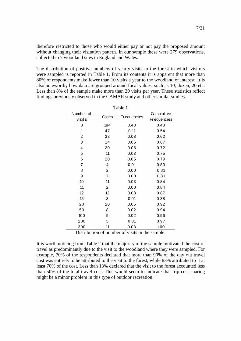
therefore restricted to those who would either pay or not pay the proposed amountwithout changing their visitation pattern. In our sample these were 279 observations,collected in 7 woodland sites in England and Wales. The distribution of positive numbers of yearly visits to the forest in which visitorswere sampled is reported in Table 1. From its contents it is apparent that more than80% of respondents make fewer than 10 visits a year to the woodland of interest. It isalso noteworthy how data are grouped around focal values, such as 10, dozen, 20 etc.Less than 8% of the sample make more than 20 visits per year. These statistics reflectfindings previously observed in the CAMAR study and other similar studies.

Table 1Number of

visits Cases FrequenciesCumulativeFrequencies

0 184 0.43 0.431 47 0.11 0.542 33 0.08 0.623 24 0.06 0.674 20 0.05 0.725 11 0.03 0.756 20 0.05 0.797 4 0.01 0.808 2 0.00 0.819 1 0.00 0.8110 11 0.03 0.8411 2 0.00 0.8412 12 0.03 0.8715 3 0.01 0.8820 20 0.05 0.9250 8 0.02 0.94100 9 0.02 0.96200 5 0.01 0.97300 11 0.03 1.00

Distribution of number of visits in the sample.

It is worth noticing from Table 2 that the majority of the sample motivated the cost oftravel as predominantly due to the visit to the woodland where they were sampled. Forexample, 70% of the respondents declared that more than 90% of the day out travelcost was entirely to be attributed to the visit to the forest, while 83% attributed to it atleast 70% of the cost. Less than 13% declared that the visit to the forest accounted lessthan 50% of the total travel cost. This would seem to indicate that trip cost sharingmight be a minor problem in this type of outdoor recreation.

8/31

Table 2.Percentof travel

cost Cases FrequenciesCumulative

Frequencies10 3 0.01 0.0120 14 0.03 0.0430 5 0.01 0.0540 14 0.03 0.0850 8 0.02 0.1060 11 0.03 0.1370 7 0.02 0.1480 12 0.03 0.1790 26 0.06 0.23100 328 0.77 1.00

Percent of travel cost attributed to visiting the forest.

The contingent valuation questions used a follow-up format allowing for a variety ofpotential model specifications (see Haab and McConnell, 2002), such as the classicsingle bounded (Bishop and Heberlein, 1979; Hanemann 1984), the more efficientdouble bounded (Hanemann, Kanninen 1991), the more rigorous bivariate (Cameronand Quiggin, 1994) and the potentially less biased one-and-a-half-bound (Cooper,Hanemann, Signorello). For the sake of comparison with other studies in thisliterature and with the previously published EU-CAMAR studies we report here onlythe results for those specifications, which are most commonly employed in theliterature, that is the linear in the bid and log-linear in the bid single and doublebounded models. More flexible forms can also be estimable as illustrated in Scarpa etal. (2000a), however these flexible forms do not normally produce estimates whichare substantially different from those obtained with more conventional approaches. 3.1 Data from open-ended responses

In the first instance we report the statistics of the open-ended WTP responses. Meanmaximum WTP is £1.66 (standard deviation 1.4) and the median is £1.5, suggesting askewed distribution, as one would expect. The relevant frequencies of maximum WTPvalues are broken down in Table 3.

9/31

Table 3.

Pounds Cases FrequenciesCumulative

Frequencies0 73 0.17 0.17

0.5 42 0.10 0.271 91 0.21 0.48

1.5 25 0.06 0.542 98 0.23 0.77

2.5 13 0.03 0.803 36 0.08 0.88

3.5 5 0.01 0.894 26 0.06 0.965 14 0.03 0.996 2 0.00 0.997 1 0.00 1.00

7.5 2 0.00 1.00 Distribution of WTP at selected cut-off points.

The statistics in table 3 suggest that approximately 80% of respondents are willing topay less than £2.50, about one quarter is willing to pay £2 and one fifth £1. Noticethat 17% is willing to pay less than 50 pence (16.3% less than 20 pence). Perhaps, abetter description of the overall distribution can be obtained in the kernel-smoothinggraph reported in Figure 1. When maximum WTP values are stated after a sequence of dichotomous choiceelicitation questions may be subject to “anchoring”. This is a well-known effect, oftenreported in the literature and it consists of a form of dependence of the maximumWTP values on the initial bid used in the discrete-choice scenario. To test the degreeto which such dependence is present in the data we report the results of an ordinaryleast square regression of stated maximum WTP values on the initial bid-response.This is a crude way of diagnosing linear dependency and “anchoring”. As one can see from Table 4 the R2 values are very close to zero and the hypothesis ofa linear relationship can be rejected, hence suggesting that anchoring is not present inthese responses. This is suggestive that these open-ended responses could be used toderive benefit value estimates.

10/31

Table 4.

+-----------------------------------------------------------------------+| Ordinary least squares regression Weighting variable = none || Dep. var. = MAXWTP Mean= 1.660304450 , S.D.= 1.396663244 || Model size: Observations = 427, Parameters = 2, Deg.Fr.= 425 || Residuals: Sum of squares= 830.9844847 , Std.Dev.= 1.39831 || Fit: R-squared= .000000, Adjusted R-squared = -.00235 || Model test: F[ 1, 425] = .00, Prob value = .99244 || Diagnostic: Log-L = -748.0408, Restricted(b=0) Log-L = -748.0409 || LogAmemiyaPrCrt.= .675, Akaike Info. Crt.= 3.513 || Autocorrel: Durbin-Watson Statistic = 1.56260, Rho = .21870 |+-----------------------------------------------------------------------++---------+--------------+----------------+--------+---------+----------+|Variable | Coefficient | Standard Error |t-ratio |P[|T|>t] | Mean of X|+---------+--------------+----------------+--------+---------+----------+ Constant 1.658892933 .16354256 10.143 .0000 BID .5702153473E-03 .60146095E-01 .009 .9924 2.4754098+---------+--------------+----------------+--------+---------+----------+

OLS regression of stated max-WTP on initial bid 3.2 Responses with zero-WTP

The 70 respondents who indicated to be unwilling to pay any of the proposed amountswere posed debriefing questions to permit the identification of true zero-WTPbehaviour. Accounting for zero-WTP is clearly important in mean and median WTPestimation (Kristrom, 1997; Strazzera et al., 2003). For example the open-ended meanWTP inclusive of zero values is £1.66, while if these are to be excluded it is £1.99. Tobe conservative it may be appropriate to use the former, but this may well be anunder-estimate of the true WTP for the individual visit. In order to investigate whether or not the zero-WTP response was genuine ordependent on the initial amount a Probit regression was estimated. This attempts toexplain the probability of a zero-WTP status on the basis of the initial bid amountpresented to the respondent. Under the hypothesis of independence the initial bidamount should not be a significant explanatory variable. The results of this regressionfrom the entire data set are reported in table 5.

Table 5. +---------------------------------------------+ | Binomial Probit Model | | Dependent variable ZERO_WTP | | Number of observations 428 | | Log likelihood function -189.3160 | | Restricted log likelihood -190.6793 | | Chi squared 2.726484 | | Prob[ChiSqd > value] = .9869634E-01 | +---------------------------------------------+ +---------+--------------+----------------+--------+---------+----------+ |Variable | Coefficient | Standard Error |b/St.Er.|P[|Z|>z] | Mean of X| +---------+--------------+----------------+--------+---------+----------+ Index function for probability Constant -1.252210390 .18290938 -6.846 .0000 BID .1072955622E-02 .65210050E-03 1.645 .0999 246.96262

11/31

As can be seen the initial bid effect is marginally significant, suggesting that zero-WTP status and initial bid are not independent. It is therefore concluded that zero-WTP probability estimates are unlikely to represent true zero-WTP, but they seem tobe statistically linked to the bid amount asked, perhaps due to protest responses. Forthis reason the issue of zero-WTP is ignored in the benefit estimation based onprobability models from discrete responses which follows. 3.3 Data from the closed-ended responses with follow-up

The budget for the additional observations was spent to sample six new sites inEngland: Sherwood (N=72), Delamere (N=58), Epping (N=76), New Forest (N=56),Dartmoor (N=55), Thetford (N=55), and one (Brenin) in Wales (N=56). The choice of sites was dictated by the need for efficient sampling. These woodlandshave a higher than average recreational use and may be thought as highlyrecreationally valuable. So, they may produce samples with higher than averagewillingness to pay for forest visits. This is the inevitable cost to pay for a cost-efficient sampling. Once the responses from those who declared they would change visiting behaviourare removed from the sample, 279 responses are left for the estimation of theprobability models from which to derive estimates of benefits. The breakdown of thedata is reported in Table 6. These values illustrate how the recorded responses areconsistent with economic theory. For example, the amount of respondents willing topay both first and second bid are reported as Yes-Yes and by and large they decline asthe bid amount increases. Similarly, the number of those who are not willing to payeither of the bid amounts presented to them (No-No) by and large increases with thebid amount.

Table 6.Bid value Yes-Yes Yes-No No-Yes No-No

£1 23 34 5 23£2 10 17 1 32£3 4 20 0 42£4 9 16 6 37

CVM Discrete choice responses 3.4 Data on forest attributes integration with previous data The new data were pooled with the old EU-CAMAR dataset and analysed jointly afterobtaining the woodland descriptors from woodland district managers and updating thebid values by the consumer purchase parity index (one 1992 GB pound is worth 1.262002 GB pound). This created a dataset of 12,185 discrete-choice CVM all linked toforest attributes.

12/31

3.5 Methodology for benefit estimation and aggregation Two methods are used to derive estimates of benefits from woodland recreation. Bothare benefit transfer methods and both are based on the benefit from a single visit. Thefirst employs a generic (site-independent) value transfer, while the second employssite-specific value estimates, constructed on the basis of woodland attributes showedto be of importance to visitors. While the generic value transfer has a history of applications in the context ofaggregate value estimates (Willis 1991), the site-dependent value transfer is arelatively new approach (Scarpa et al. 2000c), but has potentially more accuracy andit is based on a benefit value function. However, one limiting factor for itsapplicability is the availability of adequately measured site-attributes for the largenumbers of woodlands in the U.K. The approach taken here is therefore that of providing aggregate value estimates forEngland, Scotland and Wales on the basis of estimated number of visits (as reportedin the UK Leisure Day Visits, 1996, 1998). This aggregation is done prevalently usingthe generic estimate of benefit from a woodland visit, except for the few cases forwhich the relevant woodland attributes are available to enable the computation of asite-dependent estimate by means of the benefit value function. 3.6 Estimation of the generic estimate

This is based on the expected value of compensating variation and is derived viacontingent valuation method. The estimation is conducted on the basis of the datadescribed above. The open-ended data are used to derive mean, median and otherfeatures of the distribution. Because of a series of problems, amongst which lack ofincentive compatibility (respondents are thought to have incentives to provideuntruthful answers), some authors recommend to derive estimates by means ofdichotomous choice responses (Carson et al. 1999). In this report we provideestimates of expected compensating variation from both open-ended and closed-endeddata. We use both for the purpose of value aggregation, to illustrate the range ofpotential variation. From the discrete choice responses with follow-up, both single-bounded and double-bounded probability estimates are derived. The latter provide higher accuracy, butmay be prone to bias. However, some evidence seems to suggest that the efficiencygains may be higher than the risk of mis-specification (Alberini, 1995).

13/31

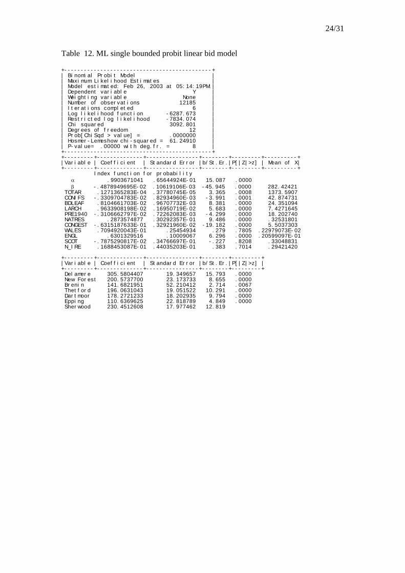
3.7 Estimation of the site-specific estimates from benefit function This estimates are derivable only on the basis of large data collected at many differentsites for which there exists site-specific attributes. Such sample size is obtained bydata pooling between the newly collected data (2002) and with the EU-CAMARcontingent valuation dataset, after up-dating bid-amounts to account for purchaseparity to 2002 pound values, as the EU-CAMAR was collected in 1992. Thisprocedure relies on the assumption of preference stability between the two momentsin time. However, this seems a defensible stance in the context of forest recreationand it appears a cost worth paying to achieve the estimation of a benefit function,which would otherwise be not available. Data for the benefit function estimation are also derived from dichotomous choicecontingent valuation responses with follow-up. As in the case of the generic estimatesthey are also derived using single and double-bounded assumptions. The single bound linear in the bid estimate from the integrated dataset is reported intable 11 along with the implied estimates of mean WTP. This provides an estimatedmean WTP of 172 pence per visit, with an approximate st. err. of 3.11 pence. The same data was employed to derive the benefit function conditional on woodlandattributes reported in Table 12. The value estimates reported show that total forestarea in hectares (TOTAR) has a positive effect on utility, along with the percentcoverage of broadleaves (BDLEAF), larch (LARCH), the presence of nature reserves(SSSI, etc.). On the other hand the marginal effect of conifers (CONIFS) and ameasure of congestion (yearly visits/car parks capacity CONGEST) are negative.While the above results are all consistent with theoretical expectations, we register anegative and significant effect of old trees (PRE1940). The dummy variables forcountries show only one significant effect, that for England, while Wales, NorthernIrish and Scottish WTP data seem not to be significantly different from the Irishbaseline

The function was then employed to predict the values of mean WTP for access at theseven newly surveyed forest sites, by applying the formula for probit models withlinear indirect utility:

�

�� ��

�

��1)( k

kkxWTPE ,

where: � denotes the constant, � denotes the marginal utility of money, k denotes thelist of forest attributes, x denotes their values, and �k the estimated parameters of theindirect utility function.

14/31

This is an illustration of the type of benefit transfer estimate that can be obtained ifwoodland attributes were made systematically available. In this illustration benefitestimates dependent on the forest attributes range from a minimum of 110 pence pervisit in Epping, to a maximum of 300 pence in Delamere.

Consider an English woodland with the following attributes: total areas in hectares =900, percent of area in conifers = 60, percent of area in broadleaves = 20, percent inlarch = 12, percent of trees planted earlier than 1940 = 5, with a nature reserve, and acongestion index of 20. This would give a value of mean WTP of per visit of 147.54pence.

This value would be obtained as follows. From table 12 � = 0.805 and � = –0.0048.The coefficients for the attributes are to be multiplied by the attribute values andadded-up, which gives:

��

��

1

,271.0k

kkx �

therefore one derives the value of:

54.1470048.0

271.0805.0)( 1�

�

���

�

��

��

�

��k

kkxWTPE pence.

4. Estimation results and aggregation

4.1 Open-ended estimates of willingness to pay

Under the assumption of random sampling the central limit theorem suggests that thelimiting distribution of the sample mean is normal. So, given the size of our sample(N= 428) we consider this property to be valid in this case, and an unbiased estimateof the mean WTP of the population of visitors is the sample mean of the stated WTPvalues. We denote this as E(WTPOE) = 1.66 pounds, with a standard deviation of 1.4.An estimate of the median or M(WTPOE) is the sample median, which is 1.5.

Open-ended responses are known in contingent valuation to produce estimates ofbenefits that are systematically lower than those produced by close-ended responses.Furthermore, some game theorists contend (Carson et al. 1999) that only dichotomouschoices have the potential to be truth-revealing mechanisms. So, our attention nowturns to this type of estimates.

4.2 Close-ended estimates of willingness to pay

These estimates are derived in 4 different forms, according to a:

a) single-bounded linear-in-the-bid model (Table 7) [SBlin]

15/31

b) single-bounded log-in-the-bid model (Table 8) [SBlog]

c) double-bounded linear-in-the-bid model (Table 9) [DBlin]

d) double-bounded log-in-the-bid model (Table 10) [DBlog]

In all these the underlying assumption is that of a random utility model. Estimateswere derived for both mean and median WTP. These vary between 2.19 (±0.30) forthe SBlin, to 2.78 (±0.10) for the DBlin, and to £ 2.75 (±0.68) for the mean of theDBlog, which also gives a media of 1.91 (±0.24).

These estimates are slightly higher than those obtained from the 1992 study. Forexample, the estimated mean WTP from a probit single bound model using all 11,906observations from 1992 (with up-dated bid values to 2002 purchase parity values)produces an estimated mean WTP of £1.71 (±0.03). This would suggest that the WTPfor a visit to woodland was higher in 2002 than in 1992.

From the close-ended analysis one is tempted to adopt the value of 2.75 as anintermediate estimates of mean WTP from the close-ended because it is generatedfrom a model with a relatively good fit, consistent with the notion of skeweddistribution of WTP, which in turns is a property consistent with the observeddistribution of household income.

4.3 Aggregation results from generic estimates

The results of aggregation are based on the number of visits estimated in the LeisureDay Visit Survey (1998), which for woodland are estimated in 346 million of trips peryear: 313 for England, 21 for Scotland and 12 million for Wales.

Using the various mean WTP estimates we obtain a range of total recreation benefitvalues for Britain, which is between a point estimate of 574 million pounds from theinference based on the open-ended CVM estimates and that of 962 million poundsfrom the highest of the close-ended CVM estimates.

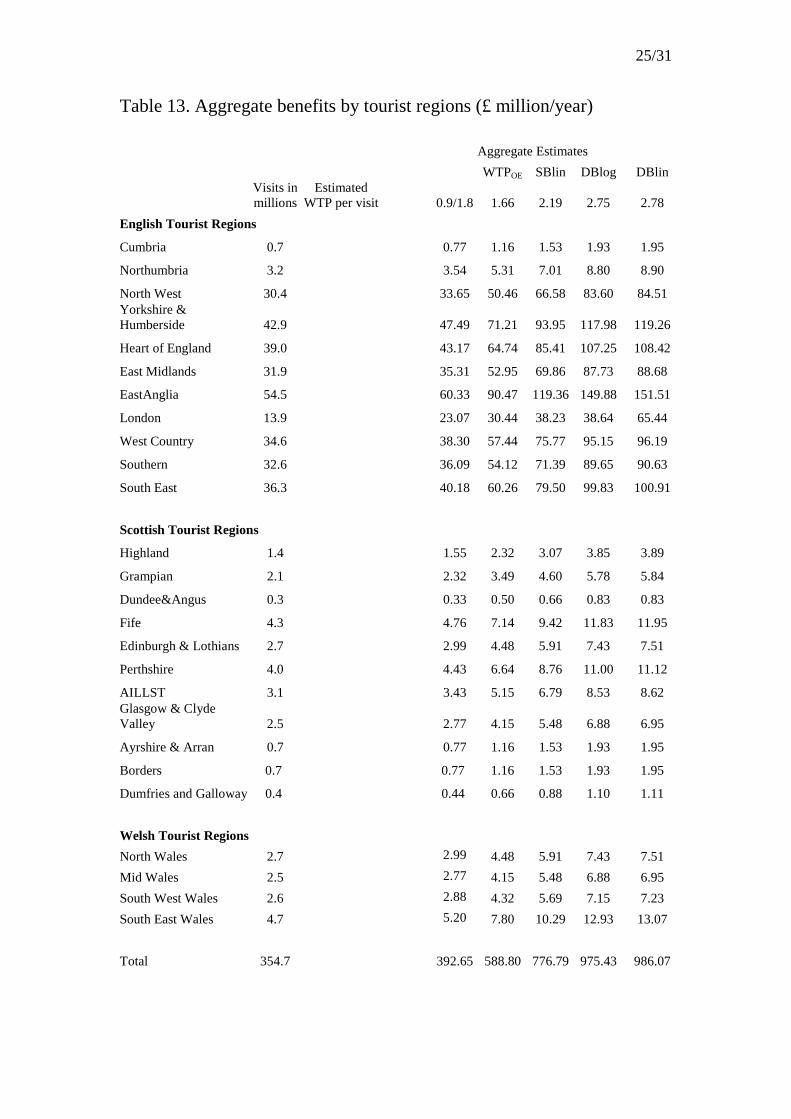
Breakdowns of the benefit estimates by tourist region are reported in Table 13, whilethose by Government Office Regions are reported in Table 14.

It is important to appreciate that the validity of the aggregate estimates relies on theassumption that both the Day Visit Survey and the surveys conducted for this forestrecreation study relate to the same type of visit, which we define here as purposefulwoodland visits. There is evidence that a number of woodland visit types may well beassociated with lower WTP values for the marginal visit than those estimated here.For example, Willis and Garrod (1991b) find that dog walkers have lower consumersurplus than other visitor types. This position is supported in another study of therecreational value of woodland planted under the community woodland supplement,

16/31

where Crabtree et al. (2001) estimated that the mean use value per household (forhouseholds within 4 miles) of CWS woodland, varied from a lower bound estimate of£0.13 to an upper bound estimate of £0.56 per household per year.

It is unclear how adjustments for these lower value visits can be made in this context.I would contend that the number of pet-related woodland walks likely to be reportedas Day Visits is quite low, and an estimate of their number at the national level is alsonot available. This kind of visits have a recreational value which is not consideredhere.

On the other hand, if distance travelled is an important conditional variable in meanWTP for true day visits to woodland, as it would be theoretically plausible, thenaggregating across round-trip distance categories of visits may be seen as desirable.With this approach one can divide the woodland visits in two categories, the firstincluding round-trip travel distances below 10 miles and the second above thisthreshold. The first category would include recreational experiences to localwoodland, while the second those to more distant ones. As shown in table 15,conditional on having travelled a round-trip distance shorter than 10 miles the open-ended WTP responses show a mean WTP of £0.9 (st. dev. 1.2), while conditional on alonger trip the open-ended mean WTP is £1.8 (st. dev. 2.3).

The U.K. Day Visit Survey (Forestry Statistics 2002, Table 2.2) reports an estimate of77% as the proportion of visits falling in the first category of “short-distance” visits,which is therefore representative of a value of 273 million visit/year. Estimating theseat a mean WTP value of £0.9 produces a value of £246 million/year for this fraction.The second category of “long-distance” visits is therefore estimated at 82million/year, with an average value of £1.8, producing an additional fraction of £146million/year. This aggregation strategy produces a more realistic total estimate forwoodland recreation of £392 million/year, which at a capitalization rate of 3.5% givesan asset value for recreation of approximately just over £12,000 million. A regionalbreakdown is provided in Table 13.

Table 15.less

10 milesfrom 11

to 25 milesfrom 26

to 50 milesfrom 51 to75 miles

Mean WTP 0.9 1.5 1.8 1.8St. Dev. WTP 1.2 2 2.3 2.1

from 76 to100 miles

from 101 to150 miles

greater than150 miles

Greaterthan 10 miles

Mean WTP 2.1 2.5 2.4 1.8St. Dev. WTP 2.2 3.1 2.7 2.3

Conditional mean WTP by distance of journey

17/31

5. Conclusions

The main objective of this study was to provide an estimate of the outdoor recreationbenefits linked to U.K. woodland. Estimates were obtained from a contingentvaluation survey carried out in 2002 which involved sampling at 7 woodland sites, 6in England and one in Wales.

From these surveys we obtained both open-ended and closed-ended responses thatwere then used to derive the benefit estimates in the form of compensating variationfor foregoing a visit to the woodland. As usual, the estimated amount varies accordingto the method of estimation, ranging from a minimum of 1.66 pounds per visit fromthe open-ended responses to a maximum of 2.78 pounds per visit from the double-bounded dichotomous choice linear-in-the-bid approach.

A secondary aim was that of estimating a benefit function from which it is possible totransfer values for recreational woodland for which there is no available primary dataon visitors WTP. This was achieved by integrating old with new forest recreation datain a systematic fashion. Such benefit function predicts theoretically better as it isdependent on forest attribute with an important recreational role. An example of on-sample prediction is proposed in support of the argument that such an approachshould be used to provide more accurate estimates that account for site-specificwoodland traits.

6. Bibliography

Alberini, A., 1995. Efficiency vs Bias of WTP estimates: bivariate and interval-datamodels, Journal of Environmental Economics and Management, 29:169-180.

Bateman, I.J., Garrod, G.D., Brainard, J.S. and Lovett, A.A. 1996. Measurement,valuation and estimation issues in the travel cost method: A geographical informationsystems approach. Journal of Agricultural Economics, 47(2):191-205.

Bishop, R. C., Heberlein, T. A., 1979, Measuring Value of Extra Market Goods: AreIndirect Measures Biased? American Journal of Agricultural Economics, 61:926-930.

Cameron, T. A.nn and Quiggin, J. 1994. Estimation using contingent valuation datafrom a dichotomous choice with follow-up questionnaire, Journal of EnvironmentalEconomics and Management, 27:218-234.

Carson, R. T., Groves, T. and Machina, M. J. 1999. Incentive and InformationalProperties of Preference Questions, Paper presented at the IX Conference of theEuropean Association of Environmental and Resource Economists, Oslo 25-27 June,1999.

18/31

Caulkins, P. P., Bishop, R. C. and Bouwes, N. W., 1986. The travel cost model forlake recreation: a comparison of the methods for incorporating site quality andsubstitution effects, American Journal of Agricultural Economics, 68(2):291-297,May; (86-5)

Cooper, J. Hanemann, W., and Signorello (forthcoming) One and One-Half bids forcontingent valuation, The review of economics and statistics.

Crabtree, J. R., Chalmers, N., Thorburn, A., MacDonald, D., Eiser, D., Potts, J. andColman, D. 2001. Economic Evaluation of the Community Woodland Scheme. Macaulay Land Use Research Institute. Report to the Forestry Commission.

Haab, T. and McConnell, 2002. Valuing environmental and natural resources. EdwardElgar Publisher

Hanemann, W. M., 1984. Welfare Evaluations in Contingent Valuations Experimentswith Discrete Responses, American Journal of Agricultural Economics, 66:332-341.

Hanemann, M., Loomis, J. and Kanninen, B. 1991. Statistical Efficiency of DoubleBounded Dichotomous Choice Contingent Valuation, American Journal ofAgricultural Economics, 73:1255-1263.

Hanley, N., and Ruffell, R. 1993. The contingent valuation of forest characteristics:two approaches. Journal of Agricultural Economics, 44(2):218-229.

Hausman, J. A. 1981. Exact consumer’s surplus and deadweight loss. AmericanEconomic Review, 71(4):662-676

Hutchinson, W.G., Scarpa R., Chilton S.M., and Mc Callion, T. 2001. Parametric andnon-parametric estimates of willingness to pay for forest recreation in NorthernIreland: a multi-site analysis using discrete choice contingent valuation with follow-ups. Journal of Agricultural Economics. January, 52(1):104-122.

Hutchinson, W.G., Scarpa, R., Chilton, S. M. and McCallion, T. 2002. SpatialDistribution Versus Efficiency Effects Of Forest Recreation Policies: Using aRegional Travel Cost Model. Forthcoming in The New Economics of OutdoorRecreation. Edited by N. Hanley, D. Shaw and R. Wright. To be published by EdwardElgar.

Kristofersson, D. and Navrud, S. 2002. Validity Tests of Benefit Transfer: Are weperforming the wrong tests? Paper presentated at the 2nd World Congress forenvironmental and Resource Economists, June 24-27 2002 Monterey, California,USA.

Kriström, B., August 1997, Spike Models in Contingent Valuation. American Journalof Agricultural Economics, 79 (3): 1013-1023 (97-34)

19/31

Ni Dhubhain, A., Gardiner, J., Davis, J. Hutchinson, G. Chilton, S., Thomson, K.,Psaltopoulos, D. and C. Anderson. 1994. Final Report EU CAMAR. Contract No8001-CT90-0008. The Socio-Economic Impact of Afforestation on RuralDevelopment, by University College of Dublin, The Queens University of Belfast andUniversity of Aberdeen.

Opaluch, J. J. and Mazzotta M. J. 1992. Fundamental issues in benefit transfer andnatural resource damage assessment, in Benefit transfer: procedures, problems andresearch needs. Workshop proceedings, AERE, Snowbird, UT, June.

Randall Alan, 1994, A Difficulty with the Travel Cost Method. Land Economics,February, 70 (1):88-96 (94-8)

Scarpa, R., Chilton S. and Hutchinson, G. 2000a. Benefits From Forest Recreation:Flexible Functional Forms For WTP Distributions. Journal of Forest Economics,February, 6(1):41-54.

Scarpa, R., Chilton S., Hutchinson, G. and Buongiorno, J. 2000b. Valuing theRecreational Benefits from the Creation of Nature Reserves In Irish Forests.Ecological Economics. April, 33(2):237-250.

Scarpa, R., Hutchinson, G., Chilton S. and Buongiorno, J. 2000c. Reliability ofBenefit Value Transfers from Contingent Valuation Data with Forest-SpecificAttributes. FEEM Working Paper n. 34.00. Forthcoming in Environmental valuetransfer: issues and methods. Edited by Ståle Navrud and Richard Ready, KluwerAcademic Publisher.

Scarpa, R., Hutchinson, W. G. Chilton, S. M. and Buongiorno, J. 2000d. Importanceof Forest Attributes in the Willingness To Pay for Recreation: A Contingent ValuationStudy of Irish Forests. Forest Policy and Economics. December, 1(3-4):315-329.

Strazzera, E., Genius, M., Scarpa, R. and Hutchinson, G. 2001. The Effect of ProtestVotes on the Estimates of Willingness to Pay for Use Values of Recreational Sites,(FEEM Working Paper n. 97.01) Forthcoming in Environmental and ResourceEconomics.

Strazzera, E., Scarpa R., Calia P., Garrod G.D., and K. G. Willis. 2003. Modellingzero values and protest responses in contingent valuation surveys. AppliedEconomics, 35(2):133-138.

Willig, R. D. 1976. Consumers’ surplus without apology. American EconomicReview, 66(4):589-597

Willig, R. D. 1979. Consumers’ surplus without apology. Reply. American EconomicReview, 69(2):469-74

20/31

Willis, K. G., 1991. The Recreational Value of the Forestry Commission Estate inGreat Britain: A Clawson-Knetsch Travel Cost Analysis, Scottish Journal of PoliticalEconomy, February, 38(1):58-75.

Willis, K.G. and Garrod, G.D. 1991a. An individual travel cost method of evaluatingforest recreation, Journal of Agricultural Economics, 42(1):33-41.

Willis, K.G. and Garrod, G.D. 1991b. Valuing Open Access Recreation on InlandWaterways: on-site recreation surveys and selection effects. Regional Studies,25(6):511-524.

Willis, K.G. and Garrod, G.D. 1992. On-Site Recreation Surveys and SelectionEffects: Valuing Open Access Recreation on Inland Waterways, in Tourism and theEnvironment: Regional, Economic and Policy Issues, J. Van der Stratton and H.Briassoulis (eds.), Kluwer Academic Publishers.

21/31

Tables with model estimates

Table 7. ML estimates for single bounded linear-in-the-bid model Normal exit from iterations. Exit status=0.

+---------------------------------------------+| Binomial Probit Model || Maximum Likelihood Estimates || Dependent variable Y || Weighting variable None || Number of observations 279 || Iterations completed 4 || Log likelihood function -184.9140 || Restricted log likelihood -193.0851 || Chi squared 16.34209 || Degrees of freedom 1 || Prob[ChiSqd > value] = .5287580E-04 || Hosmer-Lemeshow chi-squared = 11.68804 || P-value= .16567 with deg.fr. = 8 |+---------------------------------------------++---------+--------------+----------------+--------+---------+----------+|Variable | Coefficient | Standard Error |b/St.Er.|P[|Z|>z] | Mean of X|+---------+--------------+----------------+--------+---------+----------+ � .5841158043 .17770661 3.287 .0010 � -.2663418255E-02 .66552759E-03 -4.002 .0001 241.93548

+-----------------------------------------------+| WALD procedure. Estimates and standard errors || for nonlinear functions and joint test of || nonlinear restrictions. || Wald Statistic = 56.44591 || Prob. from Chi-squared[ 1] = .00000 |+-----------------------------------------------++---------+--------------+----------------+--------+---------+|Variable | Coefficient | Standard Error |b/St.Er.|P[|Z|>z] |+---------+--------------+----------------+--------+---------+ mean/median 219.3105807 29.190621 7.513 .0000

22/31

Table 8. ML estimates of double-bounded linear-in-the-bid model.+---------------------------------------------+| User Defined Optimization || Maximum Likelihood Estimates || Dependent variable Function || Weighting variable None || Number of observations 279 || Iterations completed 8 || Log likelihood function 188.9092 || Restricted log likelihood .0000000 || Chi squared 377.8183 || Degrees of freedom 2 || Prob[ChiSqd > value] = .0000000 |+---------------------------------------------++---------+--------------+----------------+--------+---------+|Variable | Coefficient | Standard Error |b/St.Er.|P[|Z|>z] |+---------+--------------+----------------+--------+---------+ � 2.357012906 .25001522 9.427 .0000 � -.8472550813E-02 .90377875E-03 -9.375 .0000

+-----------------------------------------------+| WALD procedure. Estimates and standard errors || for nonlinear functions and joint test of || nonlinear restrictions. || Wald Statistic = 802.81593 || Prob. from Chi-squared[ 1] = .00000 |+-----------------------------------------------++---------+--------------+----------------+--------+---------+|Variable | Coefficient | Standard Error |b/St.Er.|P[|Z|>z] |+---------+--------------+----------------+--------+---------+ median/mean 278.1940124 9.8183789 28.334 .0000 Table 9. ML estimates of single bounded probit log-bid model+---------------------------------------------+| Binomial Probit Model || Maximum Likelihood Estimates || Dependent variable Y || Weighting variable None || Number of observations 279 || Iterations completed 4 || Log likelihood function -183.7489 || Restricted log likelihood -193.0851 || Chi squared 18.67236 || Degrees of freedom 1 || Prob[ChiSqd > value] = .1552092E-04 || Hosmer-Lemeshow chi-squared = 9.87857 || P-value= .27365 with deg.fr. = 8 |+---------------------------------------------++---------+--------------+----------------+--------+---------+----------+|Variable | Coefficient | Standard Error |b/St.Er.|P[|Z|>z] | Mean of X|+---------+--------------+----------------+--------+---------+----------+ � 3.168073299 .75939194 4.172 .0000 � -.6029472540 .14111516 -4.273 .0000 5.3519991

+-----------------------------------------------+| WALD procedure. Estimates and standard errors || for nonlinear functions and joint test of || nonlinear restrictions. || Wald Statistic = 61.99800 || Prob. from Chi-squared[ 2] = .00000 |+-----------------------------------------------++---------+--------------+----------------+--------+---------+|Variable | Coefficient | Standard Error |b/St.Er.|P[|Z|>z] |+---------+--------------+----------------+--------+---------+ mean WTP 275.2990333 63.716225 4.321 .0000 median WTP 191.3898619 24.713140 7.744 .0000

23/31

Table 10. ML double bounded probit log-bid model +---------------------------------------------+| User Defined Optimization || Maximum Likelihood Estimates || Dependent variable Function || Weighting variable None || Number of observations 279 || Iterations completed 9 || Log likelihood function 184.7613 || Restricted log likelihood .0000000 || Chi squared 369.5226 || Degrees of freedom 2 || Prob[ChiSqd > value] = .0000000 |+---------------------------------------------++---------+--------------+----------------+--------+---------+|Variable | Coefficient | Standard Error |b/St.Er.|P[|Z|>z] |+---------+--------------+----------------+--------+---------+ � 11.59133669 1.0887712 10.646 .0000 � -2.100720458 .20435137 -10.280 .0000

+-----------------------------------------------+| WALD procedure. Estimates and standard errors || for nonlinear functions and joint test of || nonlinear restrictions. || Wald Statistic = 653.42633 || Prob. from Chi-squared[ 2] = .00000 |+-----------------------------------------------++---------+--------------+----------------+--------+---------+|Variable | Coefficient | Standard Error |b/St.Er.|P[|Z|>z] |+---------+--------------+----------------+--------+---------+ mean 20554.13800 17255.924 1.191 .2336 median 249.0842318 10.937821 22.773 .0000 Table 11. ML single bounded probit linear-bid model +---------------------------------------------+ | Binomial Probit Model | | Maximum Likelihood Estimates | | Number of observations 12185 | | Log likelihood function -6587.852 | | Restricted log likelihood -7834.074 | | Chi squared 2492.444 | | Degrees of freedom 1 | | Prob[ChiSqd > value] = .0000000 | | Hosmer-Lemeshow chi-squared = 51.05100 | | P-value= .00000 with deg.fr. = 8 | +---------------------------------------------+ +---------+--------------+----------------+--------+---------+----------+ |Variable | Coefficient | Standard Error |b/St.Er.|P[|Z|>z] | Mean of X| +---------+--------------+----------------+--------+---------+----------+ Index function for probability � .8058015627 .27952601E-01 28.827 .0000 � -.4666419E-2 .10270111E-03 -45.437 .0000 282.42421 Mean(WTP) 172.6808971 3.1159186 55.419 .0000

24/31

Table 12. ML single bounded probit linear bid model

+---------------------------------------------+| Binomial Probit Model || Maximum Likelihood Estimates || Model estimated: Feb 26, 2003 at 05:14:19PM.|| Dependent variable Y || Weighting variable None || Number of observations 12185 || Iterations completed 6 || Log likelihood function -6287.673 || Restricted log likelihood -7834.074 || Chi squared 3092.801 || Degrees of freedom 12 || Prob[ChiSqd > value] = .0000000 || Hosmer-Lemeshow chi-squared = 61.24910 || P-value= .00000 with deg.fr. = 8 |+---------------------------------------------++---------+--------------+----------------+--------+---------+----------+|Variable | Coefficient | Standard Error |b/St.Er.|P[|Z|>z] | Mean of X|+---------+--------------+----------------+--------+---------+----------+ Index function for probability � .9903671041 .65644924E-01 15.087 .0000 � -.4878949695E-02 .10619106E-03 -45.945 .0000 282.42421 TOTAR .1271365283E-04 .37780745E-05 3.365 .0008 1373.5907 CONIFS -.3309704783E-02 .82934960E-03 -3.991 .0001 42.874731 BDLEAF .8104661703E-02 .96707732E-03 8.381 .0000 24.351094 LARCH .9633908198E-02 .16950719E-02 5.683 .0000 7.4271645 PRE1940 -.3106662797E-02 .72262083E-03 -4.299 .0000 18.202740 NATRES .2873574877 .30292357E-01 9.486 .0000 .32531801 CONGEST -.6315187633E-01 .32921960E-02 -19.182 .0000 5.5037303 WALES .7094920043E-01 .25454934 .279 .7805 .22979073E-02 ENGL .6301329516 .10009067 6.296 .0000 .20599097E-01 SCOT -.7875290817E-02 .34766697E-01 -.227 .8208 .33048831 N_IRE .1688453087E-01 .44035203E-01 .383 .7014 .29421420

+---------+--------------+----------------+--------+---------+|Variable | Coefficient | Standard Error |b/St.Er.|P[|Z|>z] |+---------+--------------+----------------+--------+---------+ Delamere 305.5804407 19.349657 15.793 .0000 New Forest 200.5737700 23.173733 8.655 .0000 Brenin 141.6821951 52.210412 2.714 .0067 Thetford 196.0631043 19.051522 10.291 .0000 Dartmoor 178.2721233 18.202935 9.794 .0000 Epping 110.6369625 22.818789 4.849 .0000 Sherwood 230.4512608 17.977462 12.819

25/31

Table 13. Aggregate benefits by tourist regions (£ million/year)

Aggregate EstimatesWTPOE SBlin DBlog DBlin

Visits inmillions

EstimatedWTP per visit 0.9/1.8 1.66 2.19 2.75 2.78

English Tourist Regions

Cumbria 0.7 0.77 1.16 1.53 1.93 1.95

Northumbria 3.2 3.54 5.31 7.01 8.80 8.90

North West 30.4 33.65 50.46 66.58 83.60 84.51Yorkshire &Humberside 42.9 47.49 71.21 93.95 117.98 119.26

Heart of England 39.0 43.17 64.74 85.41 107.25 108.42

East Midlands 31.9 35.31 52.95 69.86 87.73 88.68

EastAnglia 54.5 60.33 90.47 119.36 149.88 151.51

London 13.9 23.07 30.44 38.23 38.64 65.44

West Country 34.6 38.30 57.44 75.77 95.15 96.19

Southern 32.6 36.09 54.12 71.39 89.65 90.63

South East 36.3 40.18 60.26 79.50 99.83 100.91

Scottish Tourist Regions

Highland 1.4 1.55 2.32 3.07 3.85 3.89

Grampian 2.1 2.32 3.49 4.60 5.78 5.84

Dundee&Angus 0.3 0.33 0.50 0.66 0.83 0.83

Fife 4.3 4.76 7.14 9.42 11.83 11.95

Edinburgh & Lothians 2.7 2.99 4.48 5.91 7.43 7.51

Perthshire 4.0 4.43 6.64 8.76 11.00 11.12

AILLST 3.1 3.43 5.15 6.79 8.53 8.62Glasgow & ClydeValley 2.5 2.77 4.15 5.48 6.88 6.95

Ayrshire & Arran 0.7 0.77 1.16 1.53 1.93 1.95

Borders 0.7 0.77 1.16 1.53 1.93 1.95

Dumfries and Galloway 0.4 0.44 0.66 0.88 1.10 1.11

Welsh Tourist RegionsNorth Wales 2.7 2.99 4.48 5.91 7.43 7.51Mid Wales 2.5 2.77 4.15 5.48 6.88 6.95South West Wales 2.6 2.88 4.32 5.69 7.15 7.23South East Wales 4.7 5.20 7.80 10.29 12.93 13.07

Total 354.7 392.65 588.80 776.79 975.43 986.07

26/31

Table 14. Aggregate benefits by Government Office Regions.

WTP estimates in GBP

WTPOE SBlin DBlog DBlinDay visitsin millions

(1998)0.9/1.8 1.66 2.19 2.75 2.78

North East 3.20 3.54 5.31 7.01 8.80 8.90

North West 31.10 34.43 51.63 68.11 85.53 86.46

Yorkshire and Humberside 42.86 47.45 71.15 93.86 117.87 119.15

East Midlands 31.87 35.28 52.90 69.80 87.64 88.60

West Midlands 38.30 42.40 63.58 83.88 105.33 106.47

South West 35.88 39.72 59.56 78.58 98.67 99.75

Eastern 54.48 60.31 90.44 119.31 149.82 151.45

South East 68.35 75.66 113.46 149.69 187.96 190.01

London 13.94 15.43 23.14 30.53 38.34 38.75

England - Total 319.99 354.22 531.17 700.76 879.95 889.54

27/31

Figures

Figure 1

Kernel density estimate for MAXWTP

MAXWTP

.056

.112

.167

.223

.279

.0000 2 4 6 8 10-2

Den

sity

28/31

Appendix

Figure A1. Scatter plot and cumulative distribution of WTP and distance travelled

Wtp & distance of journey

0

1

2

3

4

5

6

7

8

9

1 21 41 61 81 101 121 141 161

number of people

wtp

0

50

100

150

200

250

300

350

mile

s

29/31

Figure A2. Histogram of number of visits per year by classes of travel distance.

0

10

20

30

40

50

60

70

80

90

number visits

0-4 5_9 10_19 20-29 30-39 40-49 50-59 60-69 70-85 86-120 121-199 >200

classes of miles

number of visits/miles

30/31

Table A1. Correlation among variableswtp number other vis. miles route % propo

WTP 1Party size 0.080 1

Frequency of visit -0.227 -0.172 1Distance travelled 0.273 -0.028 -0.177 1

Percent of trip cost to forest visit 0.074 -0.087 -0.017 0.281 1

Table A2. Conditional mean WTP by frequency of visit

less 2 from 2-5 from 6-10 from 11-50 greater than 50Mean WTP 2.09 1.6 1.47 1.15 0.61

St. Dev. WTP 1.52 1.42 1.34 1.04 0.80

Table A4. Conditional mean WTP by size of visiting party

less or equal 2 from 3 to 5 from 6 to 10 more than 10Mean WTP 1.51 1.65 1.78 1.77

St.Dev. WTP 1.97 2.17 2.29 2.32