Banque de France Working Paper #735 October 2019

The Real Effects of Checks and Balances: Policy Uncertainty and

Corporate Investment Anne Duquerroy1

October 2019, WP #735

ABSTRACT

This article explores the economic effects of checks and balances on corporate investment and employment. I use U.S. gubernatorial election results from 1978 to 2010 as a source of exogenous variation in whether the party controls both the executive and the legislative branch (unified government) or not (divided government), which determines its ability to implement its political agenda. I find that both public and private firms respond to the political cycle by reducing investment and hiring when government becomes unified. Investment drops by three to five percent in the year following an election resulting in unified government, while stock returns volatility is three percent higher. The findings support the hypothesis that moving from divided to unified government raises policy uncertainty by increasing the probability of future policy changes. Consistent with a real option channel, the effect is stronger for capital intensive firms with lower asset redeployability.

Keywords: Investment, Checks and balances, Divided government, Gubernatorial elections, Political uncertainty

JEL classification: E22 ; E66 ; G18 ; G31 ; G38 ; H75

1 Banque de France : anne.duquerroy@banque-france.fr I thank Ethan Kaplan and William Mullins for extensive advice and support. I thank Philippe Aghion, Francesco d’Acunto, Vincent Bignon, Alan Drazen, Michael Faulkender, Laurent Frésard, Frances Lee, Mathias Lé, Nicholas Magnan, Maurizio Montone, N. Prabhala, Jacopo Ponticelli, Farzad Saidi, Frédérique Savignac, Liu Yang and participants at the Maryland Political Economy group, Maryland Finance brownbag, AFSE, Banque de France seminar, 26th Finance Forum and MFA 2019. I am grateful to Don Bowen for helping scrape the 10K data. The views in this paper may not reflect those of the Banque de France or the Eurosystem.

Banque de France Working Paper #735 ii

NON-TECHNICAL SUMMARY

In the wake of the political crisis the U.S. experienced in 2019, which led to a month long partial shutdown of the federal government in January, the question of the economic consequences of having a government controlled by a single party or not - i.e. unified versus divided government - has been widely debated. This question is not specific to the U.S. Several European countries including Germany or Italy have also experienced divided legislatures and the need to form coalition governments in recent years. The concept of divided /unified government is central to lawmaking because the extent to which a given party fully controls the government affects its ability to pass bills. This ability is materially greater when the elected government is unified. As the likelihood of significant policy changes increases so does policy uncertainty surrounding such changes: uncertainty about which policies will be introduced, about when those policies will be introduced and about the effects of those policies. By contrast, electing a divided government leads to more moderate (economic) policies and a lower probability of significant policy changes. This paper examines the economic effects of having a unified or a divided government through the lens of policy uncertainty. In particular, I use the elections of U.S. governors (“gubernatorial elections”) as a source of variation in divided or unified government, to help isolate the effect of a political transition from other confounding factors. My main empirical design exploits the fact that gubernatorial elections in different states occur in different years. This creates changes in divided or unified government, which are staggered over time and across states, for a difference-in-differences research design in which I compare firms headquartered in states that switch to unified or to divided government, with firms headquartered in states that do not experience any changes. In additional results, I use a regression discontinuity design, for a subsample of close elections. I exploit the pseudo-random variation regarding which party wins elections in close races, by comparing those states that became unified because a governor candidate barely won an election and those that stayed divided because a governor candidate barely lost an election. I document novel and robust evidence that transitions between divided and unified government induce cycles in corporate investment and employment. Specifically, in the year following an election, the corporate investment rate of firms headquartered in states that switch to unified government drops by an average of three to five percent, relative to other firms (see figure). On the employment side, the job creation rate also decreases. The effect is entirely concentrated in the first year after a governor is elected, which is consistent with firms postponing (partially) irreversible investment decisions in presence of uncertainty. The effect is stronger for smaller firms and firms whose operations are concentrated in their state of headquarters, which are more exposed to local policy. The effects of transitions to divided government on corporate investment are weakly positive; they vary over time conditional on political polarization and can even turn into significantly negative in states where Republican and Democratic party platforms are most ideologically divergent. This suggests that the status quo becomes an undesirable outcome when political polarization is too high - as gridlock will likely dominate any political compromise attempts. Finally, higher stock returns volatility for firms headquartered in states switching to unified government, combined with higher - negative - sensitivity of investment for capital intensive firms with lower asset redeployability, support the hypothesis that changes in partisan control translate into changes in the degree of policy uncertainty. My findings suggest that partisan alignment between executive and legislative powers may be as relevant to explain corporate outcomes as partisan preferences over policy through the

Banque de France Working Paper #735 iii

channel of policy uncertainty. More broadly, these results highlight the interplay between political institutions and corporate decisions and the possibility that checks and balances directly influence firm behavior.

Firm investment rate in post-election year Averages of investment rate as a function of electoral margin

Source: Duquerroy (2019)

Les effets réels du partage des pouvoirs : incertitude politique et investissement des

entreprises RÉSUMÉ

Cet article étudie les effets économiques du partage des pouvoirs sur l'investissement et l'emploi des entreprises. Il utilise les résultats des élections des gouverneurs aux États-Unis, de 1978 à 2010, comme source de variation au fait qu’un même parti politique contrôle simultanément le pouvoir exécutif et le pouvoir législatif (gouvernement unifié) ou non (gouvernement de coalition). Le passage à un gouvernement unifié conduit à un déclin temporaire de l’investissement et du taux de création d’emplois, l’année qui suit l’élection, tandis que la volatilité des rendements boursiers augmente. Les résultats sont en adéquation avec le fait que l’élection d’un gouvernement unifié accroit l'incertitude politique en augmentant la probabilité de changements politiques futurs. En ligne avec la théorie de l’investissement comme option réelle, l'effet est plus marqué pour les entreprises à forte intensité en capital dont les actifs sont plus difficilement redéployables.

Mots-clés : Investissement, Contre-pouvoirs, Coalition, Élections, Incertitude politique.

Les Documents de travail reflètent les idées personnelles de leurs auteurs et n'expriment pas nécessairement la position de la Banque de France. Ils sont disponibles sur publications.banque-france.fr

1. Introduction

In the wake of the high profile political crisis the U.S. experienced in 2019, which led

to a month long partial shutdown of the federal government in January, the question of

the economic consequences of having a government controlled by a single party or not -

i.e. unified versus divided government - has been widely debated. Political gridlock is not

specific to the U.S.. Europe has had its own episodes including Germany’s inability to form

a coalition government following their September 2017 election and Spain’s nearly year-long

failure to elect a working government in 2016. However, this absence of political leadership

did not prevent the Spanish economy to grow strongly in 2016 and its unemployment rate

to decline1. This paper examines the economic effects of checks and balances. While the

Democratic and Republican parties have different political agendas, the concept of unified

government is important to state lawmaking because the Governor, the Senate and the House

all play decisive roles in turning a partisan agenda into state legislation. Many policies, and

in particular tax policies, require Congressional approval. Whether a given party fully con-

trols the government affects its ability to pass bills, and this ability is materially greater

when the elected government is unified. 2

This paper investigates the causal link between checks and balances and corporate in-

vestment and employment cycles. First, I show how corporate investment and employment

respond to changes in government party control, and more specifically in moves from a di-

vided to unified government (and the reverse), at the state level. Then I test whether policy

uncertainty is the channel driving the effects.

There are several empirical challenges in causally estimating the effect of political cycles1Economic growth remained robust with activity growing at an annualized 3.2% rate in 2016. The

unemployment rate declined, but remains high, at about 19%. Source: OECD2A unified government is not a sufficient condition for all legislation to be passed, as supermajority

requirements (such as 2/3 or 60 percent) exist for some legislation in legislative bodies.

1

on firm behavior. First, analysis at the federal level is not possible due to the low number of

presidential elections. Shifting the analysis to the state level, however, allows me to use data

from gubernatorial elections, while still observing a set of states under a common legal and

regulatory system and sharing many institutional features. State governments affect firms in

many ways, for instance by levying taxes, providing subsidies and local business incentives

and by defining labor and environmental policies. Second, election results are endogenously

correlated with current fluctuations in economic activity, as well as with anticipated changes

in economic conditions that independently affect corporate decisions. To control for first

moment effects induced by the current state of the economy, this paper takes advantage of

variation in when gubernatorial elections in the U.S.take place. The timing of elections is

exogenously determined by the political calendar of each state, mitigating endogeneity con-

cerns that changes in investment in the post-election year may systematically be induced by

fluctuations in business cycle. In addition, gubernatorial elections in different states occur

in different years and, for all but nine states, they are not concurrent with Presidential elec-

tion years.3 As a result gubernatorial electoral outcomes are spread across time and across

states. In this paper I use the outcomes of 358 gubernatorial elections held between 1978

and 2010 in 46 states. These elections led to 53 staggered switches from divided to unified

governments and 46 switches from unified to divided governments.

To establish the causal effects of a shift to or from unified government on corporate de-

cisions, I first use a difference-in-differences estimation strategy to leverage these staggered

switches across time and states to help isolate the effect of a political transition from other

confounding factors. I start by examining corporate investment sensitivity to switches from

and to divided government. Controlling for standard proxies for investment opportunities3The following states have concurrent Governor and Presidential elections: Delaware, Indiana, Missouri,

Montana, North Carolina, North Dakota, Utah, Washington, and West Virginia.

2

(Tobin’s Q and cash flows), demand (sales growth), state-level economic conditions (GDP

growth and unemployment rate) and partisan effects (party of the incumbent or elected gov-

ernor, incumbency advantage, change in partisan majority, among others), I find evidence of

a negative relationship between switches from divided to unified government and investment.

Specifically, in the year following an election, corporate investment rate drops by an average

of three percent when government switches from divided to unified, compared to when no

shift occurs. This is consistent with a raise in policy uncertainty when government switches

to unified, as the likelihood of policy changes increases. On the contrary switching to divided

government brings status quo and thus a lower probability of significant policy changes. The

effects of transitions from unified to divided government on corporate investment, however,

are less clear-cut. They vary over time, conditional on political polarization, from positive

- though non-significant - to significantly negative in times of higher political polarization.

Consistent with the status quo becoming an undesirable outcome when political polarization

is too high - as gridlock will likely dominate any political compromise attempts - a switch

to divided government is associated with a drop in the investment rate only in states where

Republican and Democratic party platforms are most ideologically divergent.

Second, I use a regression discontinuity design to address remaining identification con-

cerns. First, there could be an omitted variable bias such that unobserved state-level eco-

nomic conditions or anticipated state-level economic conditions are driving both the election

outcomes and the investment cycle. Second, the difference-in-differences specification may

not capture the full effect of switching when transitions are correctly and easily anticipated

leading firms to take corrective actions ex-ante such as shifting investment from one state

to another, biasing firm-level result towards zero (Falk and Shelton, 2018). The RD design

exploits the pseudo-random variation regarding which party wins elections generated by the

uncertainty of close races. Thus, for the sub-sample of states that were divided ex-ante, those

states that became unified because a governor candidate barely won an election and those

3

that stayed divided because a governor candidate barely lost an election should be close to

identical, except for dimensions that are directly affected by the election outcome. Focusing

on these close elections therefore allows me to estimate the local causal effect of a switch

in divided/unified government, as determined by the party of the governor. One caveat of

this analysis is that there are only a limited number of such elections (between 33 to 53

depending on the bandwidth chosen for the analysis). The RD estimates show that giving a

single party full control over a state by winning the governorship systematically leads to a

significant drop of minus 4.5 percent in the investment rate of firms headquartered in that

state in the post-election year. The switch from a unified to a divided government does not

significantly impact the investment rate of firms headquartered in switching states relative

to firms that are not. Taken together these results fully support the conclusions from the

difference-in-differences analysis.

Next, I explore how state-level exposure mediates the effect. Because the reach of state

policy is local, identifying firms or industries which are more exposed to their home state’s

policies is critical to identifying the potential effects and the channels through which state

policy affects corporate decision making. Because Compustat firms are generally multi-state

firms, their exposure to their headquarters-state policy is lower than for single-state firms.

To address this concern I report results from difference-in-differences regressions for smaller

firms, which are more likely to be geographically concentrated in their home state (Jens,

2017). I also use the main state of operations as an alternative to the state of headquarters,

based on García and Norli (2012) textual analysis data. In addition to geographic exposure,

smaller firms may also be more sensitive to political risk as they are less likely to engage into

lobbying efforts, contrary to larger firms that have been shown to actively manage political

risks in this way (Hassan et al., 2019). Results are stronger, with a drop in the post-election

year investment rate that is twice as large as the average effect for these firms.

Finally I extend the analysis to private firms, using employment data from the Census

4

Bureau’s Business Dynamics Statistics. I find a positive effect of a switch to divided govern-

ment on the job creation rate and a negative effect in the job creation rate following a switch

to unified government. The economic magnitude of the drop is weaker than for investment,

and translates into a 1.7% decrease in the gross job creation rate. The job destruction rate is

also negatively affected by switching to unified government (though the effect is not consis-

tently statistically significant) so that the net creation rate remains essentially unchanged.

This suggests a wait-and-see effect. The results are consistent with the findings of Barrero,

Bloom, and Wright (2017) which show that investment is more sensitive to long-run policy

uncertainty than hiring.

Next, I turn to the mechanism through which this effect could be working, and present

evidence consistent with the policy uncertainty channel. Government policy, including state-

level policy, represents a major source of uncertainty for many firms, as changes to laws and

regulations impact profits and operations (cf. examples of 10-K citations from the risk factors

sections cited in Section 1). In fact, a growing literature examines the relationship between

policy uncertainty and either corporate investment (Jens, 2017; Julio and Yook, 2012; Gulen

and Ion, 2016; Barrero, Bloom, and Wright, 2017) or asset prices (Kulatilaka and Perotti,

1998; Pástor and Veronesi, 2013; Kelly, Pástor, and Veronesi, 2016).

While this paper aims at identifying the impact of the likelihood of a policy change

depending on the election outcome, it cannot disentangle between the different sources of

uncertainty. There are in principle (at least) four sources of uncertainty resulting from a

unified government: (1) uncertainty about which policies will be introduced, (2) uncertainty

about the specifics of those policies, (3) uncertainty about when those policies will be intro-

duced and (4) uncertainty about the effects of those policies. Since voters know the elected

governor’s political agenda,uncertainty about which policies will be introduced is likely lower

in a unified government. The last three sources of uncertainty will therefore dominate and

5

the effects of policy content uncertainty and policy timing uncertainty should be transitory.

For example, when Donald Trump was elected President in 2016 with Republicans control-

ling the Congress, there was low uncertainty about the likelihood of future corporate tax

cuts. However, the details of this reform were not clear, especially as two different tax plans

were on the table at that time - the Trump campaign one and the corporate tax plan from

the House Republicans (Wagner, Zeckhauser, and Ziegler, 2018). The timeline of the reform

was also unknown. In addition, as American politics is polarized, unified governments are

likely to yield strong partisan outcomes in the form of more extreme economic policy choices,

the effects of which may be more difficult to apprehend. An example of such choices can

be found in the Kansas experiment under the unified government of Republican Governor

Brownback, whose administration enacted a major tax cut for individuals and businesses.4

A switch to a unified government may thus raise policy uncertainty in general by increas-

ing the propensity to reform, and making likely reforms more radical and more polarized. As

a result, policy uncertainty is very likely to be higher in a post-election year when govern-

ment switches to unified government relative to other post-election outcomes. By contrast,

electing a divided government has been theorized as a way for voters to get middle-ground

policy through institutional balancing (Alesina and Rosenthal, 1996). In addition, because

passing legislation requires bipartisan support under divided government, policy decisions

are more likely to be durable and to survive majority changes. In case no cooperative equi-

librium is reached, however, the default option is the status quo. Conflict between opposing

parties in a divided government has been shown to increase the likelihood of stalemate in the

policy making process in many cases (Binder, 2003; Bowling and Ferguson, 2001; Kirkland

and Phillips, 2018), though these results vary depending on how legislative accomplishments4With Brownback as governor, Kansas is in the midst of a self-described economic experiment, a project

that, whatever you think of its merits, is one of the boldest and most ambitious agendas undertaken by anypolitician in America. Brownback calls it the march to zero, an attempt to wean his stateâs government offthe revenues of income taxes and transition to a government financed entirely by what he calls consumptiontaxes that is, sales taxes and to a lesser extent, property taxes. New York Times, August 05 2015.

6

are measured (Mayhew, 1991 vs. Binder, 2003) or the type of outcome, e.g. fiscal (Alt

and Lowry, 1994) vs. welfare policy (Bernecker, 2016) and fail to address the issue of the

endogenous nature of a political agenda. Gridlock in divided government is consistent with

the literature on decision making in political systems with veto players, which shows that

the potential for policy change decreases as the number of groups with institutional veto

power increases (Tsebelis, 1995). Stability and smaller policy shifts are preferable for both

investors and firm managers because uncertainty about the future has real effects on eco-

nomic agents’ behavior (Bernanke, 1983; Bloom, 2009, Bloom, Bond, and Van Reenen, 2007;

Pindyck, 1991).5 Indeed when investment is at least partially irreversible, uncertainty creates

incentives to postpone investment decisions.6

Exploring the time dynamics of the sensitivity of investment to switches from divided

to unified government, I find that the effect is entirely concentrated in the first year after a

governor is elected. This result is consistent with the wait-and-see approach suggested by

the policy uncertainty channel. In the second and third year, uncertainty about government

policies is more likely to have fallen, while some of the effects of early measures may already

have materialized.

An analysis of firm-level volatility supports this view. Total realized volatility is three

percent higher in the first year of a governor’s term for firms headquartered in states that

switch to unified government relative to other firms, providing evidence of the importance of

the policy uncertainty channel. Finally, I test whether firms that are ex-ante more sensitive

to uncertainty respond more strongly than other firms do, to switches to unified govern-5Now with Democrats controlling the House of Representatives, the GOP increasing its majority in the

Senate and President Trump in the White House, it will be nearly impossible to pass anything remotelycontroversial. That will drive many people crazy, but markets love it. We should now have a long stretchwhere political risks go way down, which should be good for stocks. Financial Times, November 7 2018.https://www.ft.com/content/390b5982-e263-11e8-a6e5-792428919cee

6Note that, as underlined by Julio and Yook, 2012, incentives to wait arise even if a "bad" policy outcomeis not likely. Even a positive change in policy, by reordering the ranking of the expected returns of mutuallyexclusive projects, can affect how the firm allocates its investment spending.

7

ment and to divided government. Using firm-level asset redeployability from Kim and Kung

(2016) and cyclicality (durable vs. non durable goods), I find that the magnitude of the

effect of a switch to unified government is three to five times stronger for firms characterized

by a higher degree of investment irreversibility. This finding supports the hypothesis that

switches to unified governments translate into an increase in the degree of policy uncertainty.

The article proceeds as follows. Section 2 reviews the literature. Section 3 describes how

state policy matters for corporate decisions and section 4 describes the data and sample. Sec-

tion 5 discusses the empirical strategy. Section 6 presents the main empirical results. Section

7 investigates the policy uncertainty channel by looking at firm stock returns volatility and

cross-sectional heterogeneity in the response of firm investment to changes in government

unification. Section 8 concludes.

2. Related literature

This paper is directly related to the large literature on the real effects of political in-

stitutions. The effect of institutions on investment is an important element of this re-

search agenda, dominated by cross-country studies on cross-border capital flows (e.g. Al-

faro, Kalemli-Ozcan, and Volosovych, 2008; Besley and Mueller, 2017). Here, I focus on

U.S.institutions and corporate investment by U.S.public firms. In particular, I provide a

new perspective on the economic effects of checks and balances by showing that corporate

investment responds negatively to transitions from divided to unified governments, providing

novel evidence that unified government temporarily discourages investment by raising policy

uncertainty.

This paper also relates to the literature on the effects of politics on real and financial

outcomes. The earlier literature focuses on the impacts of politics on the macroeconomy

8

(see Drazen, 2001, for a survey), showing strong evidence of partisan business cycles in the

U.S.(Alesina and Sachs, 1988; Alesina, Roubini, and Cohen, 1997). Empirical regularities of

partisan cycles have also been documented in the finance literature with excess returns in

the stock market being significantly higher under Democratic than Republican presidencies

(Santa-Clara and Valkanov, 2003).7 Complementary to investigating the relationship be-

tween politics and finance through the lens of partisanship, my research takes into account

the fact that the party of the winner of the election does not necessarily fully control policy

and focuses on the ability of a government to implement its political agenda.

A recent micro-based literature explores a variety of underlying channels which can drive

a causal effect of political cycles on financial markets and firm-level outcomes. Govern-

ment spending (Belo, Gala, and Li, 2013), campaign contributions (Cooper, Gulen, and

Ovtchinnikov, 2010; Akey and Lewellen, 2017), changes in the degree of political connected-

ness (Faccio, 2006; Fisman, 2001) and political uncertainty (Julio and Yook, 2012) have been

shown to matter in explaining how political cycles influence.8 9 I document novel and robust

evidence that corporate allocation decisions are impacted by checks and balances. Switches

from divided to unified governments, and from unified to divided government, induce cycles

in corporate investment and employment.

This article also contributes to the political economy literature on the consequences of

divided government. Empirical evidence on the economic consequences of divided govern-7From 1927 to 1998 Santa-Clara and Valkanov (2003) find that average excess returns in the U.S.stock

market are 9% to 16% higher under Democratic than Republican presidencies. Neither business cycles northe difference in the riskiness of the stock market explain this relationship. Pástor and Veronesi (2017) offeran explanation by modelling how political cycles generated by time-varying risk aversion can explain whyaverage returns are higher under Democratic presidencies.

8Belo, Gala, and Li, 2013 show that, conditional on the presidential partisan cycle, firm exposure togovernment spending predicts the cross section of stock returns.

9Cooper, Gulen, and Ovtchinnikov (2010) show that corporate contributions, in particular the numberof candidates supported by a firm, are positively correlated with future excess returns. Akey and Lewellen(2017) investigates the value of firm political connections in a sample of close, off-cycle U.S. congressionalelections and finds that post-election abnormal equity returns are 3% higher for firms donating to winningcandidates relative to firms donating to losing candidates.

9

ment is scarce. The literature has almost exclusively focused on propensity to reform, with

mixed findings. Its findings are very sensitive to the way reforms are defined and measured,

and fail to address the issue of the endogenous nature of the political agenda. Responding to

Mayhew’s Divided We Govern claim (Mayhew, 1991), a subsequent body of empirical works

suggests that meaningful legislation is less likely to pass under divided than unified govern-

ment (Binder, 2003; Bowling and Ferguson, 2001; Coleman, 1999; Howell, Adler, Cameron,

and Riemann, 2000). Coleman (1999) and Howell et al. (2000) find evidence supporting the

conjecture that in the US, at the federal level, unified government is much more productive

with respect to the quantity of important legislative enactments. At the state level, consis-

tent with the gridlock hypothesis, Bowling and Ferguson (2001) find that when a governor

faces a legislature controlled by the opposition party, divided government does make passage

of controversial policy more difficult. Andersen, Lassen, and Nielsen (2012) finds that the

state budget is 10 to 20% more likely to be late under divided government. Focusing exclu-

sively on welfare reforms, Bernecker (2016) offers counter-intuitive empirical evidence that

welfare reforms in U.S.states are more likely to be adopted under divided governments, as

well as after a switch to a divided government. Though it is hard to generalize such findings

to a broader range of political issues, the results underline how difficult it is to disentangle

the effects of divided government looking at legislative outcomes such as reforms or waiver

adoption when the political agenda itself is endogenous to the type of government.10 My

paper offers an indirect test of how a unified or divided government affects state policy by

looking directly at firms’ decisions - which stand to be affected by policy changes - under

changes in divided or unified government. To the best of my knowledge, the question of how

divided vs. unified affects corporate decisions has not been explored.10Welfare policy changes were mainly concentrated in the mid-90s, at a time of bipartisan consensus on

the need to adopt restrictive welfare reforms. These findings do not rule out that most contested issues maybe less likely to be on the political agenda of divided governments and that gridlock may be more likely tohappen when such controversial issues are on the agenda.

10

Finally this paper relates to the literature on the real and financial effects of uncer-

tainty. Various theoretical models (e.g. Bernanke, 1983; Bloom, Bond, and Van Reenen,

2007; Bloom, 2009) show that if investment projects are not fully reversible, firms become

cautious in the presence of uncertainty and temporarily hold back on investment until more

information is revealed. Longer precautionary delays result from the fact that uncertainty

increases the value of the option of waiting to invest (Pindyck, 1991). Policy uncertainty in

particular has received a lot of interest lately with a growing literature looking at the rela-

tionship between policy uncertainty and corporate investment (Julio and Yook, 2012; Gulen

and Ion, 2016) or asset prices (Pástor and Veronesi, 2013; Kelly, Pástor, and Veronesi, 2016).

A number of articles have used national elections (e.g. Julio and Yook, 2012; Durnev, 2010;

Kelly, Pástor, and Veronesi, 2016) as well as U.S.gubernatorial elections (Gao and Qi, 2013;

Colak, Durnev, and Qian, 2017; Jens, 2017; Falk and Shelton, 2018) to identify plausibly

exogenous variations in uncertainty surrounding the election results. Policy uncertainty is

found to command a risk premium embedded in asset prices11 and electoral uncertainty

temporary depresses corporate investment (Julio and Yook, 2012)12. The papers closest to

this paper are Jens (2017) and Falk and Shelton (2018) which show a decline in corporate

investment in reaction to electoral uncertainty surrounding U.S.gubernatorial elections. Jens

(2017) documents that high electoral uncertainty causes lower investment in gubernatorial

election years. She finds that firms headquartered in states with a gubernatorial election in

the following quarter cut investment by 5% relative to firms in states that do not elect a

governor. Investment rebounds in the following quarter if an incumbent is re-elected. Falk

and Shelton (2018) combine measures of electoral uncertainty and of ideological distance

between parties to show how businesses respond to policy uncertainty around elections by11Municipal bond yields rise around U.S. gubernatorial elections (Gao and Qi, 2013); Short-maturity put

options spanning political events have a higher price than comparable ones that do not (Kelly, Pástor, andVeronesi, 2016).

12Julio and Yook (2012) document that high electoral uncertainty causes lower investment in electionyears. They find that firms cut investment by 4.8% relative to non-election years, on average.

11

permanently shifting manufacturing investment from one state to another. My paper goes

beyond looking at the effects of electoral uncertainty by investigating how political insti-

tutions affect investment. I differentiate my work by focusing on post-election uncertainty

about the likelihood and the impact of future policy changes. This probability is directly

tied to the extent to which a single party controls the government.

3. State government and state policy

3.1. State government and state election cycle

Like the federal government, each U.S.state government is made of a legislative and an

executive branch. All state legislatures but Nebraska, are divided into a lower and an upper

chamber. They have members elected by voters every two to four years. Party control of

state government can exist in various configurations. A government is divided if at least the

majority in one of the legislative chambers is from a different party than the governor’s party.

Divided government can occur in a split branch form, when the legislature is unified against

the executive, as it was the case for the U.S.Congress at the federal level after Republicans

regained a majority in the Senate after 2014 mid-term elections. Divided government may

also mean that the legislature is itself divided (so called split legislature) as it was the case

at the federal level, right before the 2014 mid-terms, with Republicans holding the House

and Democrats the Senate.

Currently forty-eight states have four-year terms for their governors (Vermont and New

Hampshire have a two-year term. Arkansas before 1986 and Rhode Island before 1994

also did.). Though the four-year length of a gubernatorial term is the same, states hold

their elections in a staggered way. Thirty-four states hold their gubernatorial elections

in even numbered years not concurrent with Presidential elections, nine states hold their

12

gubernatorial elections in the same year as presidential elections.13 Three states hold their

gubernatorial elections in the year before the Presidential election (Kentucky, Louisiana,

and Mississippi) and two (New Jersey and Virginia) hold them in the year after. With the

exception of Louisiana, gubernatorial elections always take place on the first Tuesday in

November.14

3.2. State policy matters

US state governments have substantial power in shaping the economic environment in

which firms operate. State-specific tax and labor regulations and business incentive policies

directly affect corporate profitability. Legislatures in most states (thirty four states plus the

District of Columbia) can approve tax bills with a simple majority vote in each house and

state taxes account for about 20% of total corporate income tax paid (Heider and Ljungqvist,

2015). Most states have industry specific or targeted programs designed to incentivize in-

vestment within the state (for example, aimed at green energy technology). Minimum wage

laws and regulations on collective bargaining, which affect labor costs, also vary at the state

level. Anecdotal evidence such as the January 2015 decision of Daimler AG to relocate its

Mercedes-Benz USA headquarters from New Jersey to an Atlanta suburb illustrates the rel-

evance of state politics to corporate decisions, with firms willing to take advantage of low

union membership in right-to-work states and lower corporate taxes. Serfling (2016) finds

that higher firing costs embedded in state-level labor protection laws lower financial leverage

of firms headquartered in these states. The impact of state-level policies on corporate deci-13Alabama, Alaska, Arizona, Arkansas, California, Colorado, Connecticut, Florida, Georgia, Hawaii,

Idaho, Illinois, Iowa, Kansas, Maine, Maryland, Massachusetts, Michigan, Minnesota, Nebraska, Nevada,New Mexico, New York, Ohio, Oklahoma, Oregon, Pennsylvania, Rhode Island, South Carolina, SouthDakota, Tennessee, Texas, Wisconsin and Wyoming hold gubernatorial elections in even numbered yearsnon concurrent with the Presidential election. Delaware, Indiana, Missouri, Montana, North Carolina,North Dakota, Utah, Washington, and West Virginia hold their gubernatorial elections in the same year aspresidential elections.

14Louisiana is an exception with respect to election dates that can be different because of the open primarysystem applied to gubernatorial elections.

13

sions is especially strong on smaller and less geographically diversified firms (Colak, Durnev,

and Qian, 2017; Wald and Long, 2007). Finally, state-level policy is often identified by firms

as a source of uncertainty in the risk factors section of their 10-K reports (cf. examples cited

in footnote).15

4. Data and sample

4.1. Election data and sample

This study considers 383 gubernatorial elections conducted in 46 states between 1978 and

2010 and takes into account 358 post-election years in the empirical analysis. It spans up

to nine gubernatorial elections in each state. There are 381 regular gubernatorial elections

whose timing is exogenous. Two special elections are also included. Removing them does

not change the results.16 U.S.gubernatorial election results from 1978 to 2000 have been

obtained from List and Sturm (2006). Data from 2000 to 2010 have been updated using

the Congressional Quarterly database from CQ Press Electronic Library. The data on party15INNODATA, headquartered in NJ, incorporated in DE, 10-K 2012. Provider of business process and

IT services. "Measures aimed at limiting or restricting outsourcing by U.S.companies are under discussionin Congress and in numerous state legislatures. While no substantive anti-outsourcing legislation has beenintroduced to date, given the ongoing debate over this issue, the introduction of such legislation is possible.If introduced, our business, financial condition and results of operations could be adversely affected and ourability to service our clients could be impaired"ALABAMA GAS CORP, headquartered and incorporated in Alabama, 10-K 2012. Oil & Gaz Company."Federal, state and local legislative bodies and agencies frequently exercise their respective authority to adoptnew laws and regulations and to amend and interpret existing laws and regulations. (. . . ) Currently, thereare various proposed law and regulatory changes with the potential to materially impact the Company. (. . . )Due to the nature of the political and regulatory processes and based on its consideration of existing proposals,the Company is unable to determine whether such proposed laws and regulations are reasonably likely to beenacted or to determine, if enacted, the magnitude of the potential impact of such laws (. . . )"These examples have been generated with the help of Don Bowen, by searching the body of 10-K reportsavailable in the EDGAR SEC database, for keywords related to state level policy such as "state legislature","state government", "gubernatorial elections", "Governor", "local legislative bodies", "local government".

16The 2003 California gubernatorial recall election was a special election permitted under California statelaw. It resulted in voters replacing the incumbent Democratic Governor Gray Davis with Republican ArnoldSchwarzenegger. The 2010 Utah special election was conducted to fill the remainder of Jon Huntsmanâsterm who resigned in 2009 to become the United States Ambassador to China.

14

control of state governments and legislatures have been obtained from Klarner’s dataset

on Partisan Balance of State governments (Klarner, 2013c). The final data includes the

election date, the winning governor candidate and her party, whether the incumbent governor

participates in the election, the vote margin in the gubernatorial election, the party holding

the Senate or the House and whether the government is divided.

A government is divided when all three institutions of state government (i.e., the two

chambers of the legislature and the governor’s office) are not controlled by the same party

and when there are not enough legislators to override a gubernatorial veto.17 Since I am

interested in the partisan control of state governments, I exclude Nebraska, which has a

unicameral legislature with no party affiliations. I also drop elections in which one of the top

two candidates is an independent.18 Vermont and New Hampshire have a two-year terms.

Arkansas before 1986 and Rhode Island before 1994 also did. They are excluded from my

sample in order to compare states with the same political cycle length of four year. Finally, I

am focusing on gubernatorial elections in this paper and thus considering changes in partisan

controls concurrent with gubernatorial elections, and not additional changes that may result

from mid-term legislative elections.

[Insert table 1 - Summary Statistics]

As shown in panel A of table 1 at the state level, over the 33 years of the sample period,

swings from divided to unified government are the norm and not the exception. Half of U.S.

states are divided on average between 1978 and 2010. 15% of the gubernatorial elections

considered in this study resulted in a change from a divided to a unified government (53

gubernatorial elections) while 13% (46 elections) resulted in a transition from a unified to a

divided government. In 49% of elections held between 1978 and 2010 a Republican governor17I use the "true_divided_gov_a" definition in Klarner (2013c) partisan data codebook. Results are fully

robust to the use of a looser definition (cf. table 2 column 8).18This includes Minnesota (1999-2003), Maine (1995-2003), Connecticut (1991-1995) and Alaska (1990-

1994).

15

was elected. Switches from divided to unified or from unified to divided have been frequent

and quite evenly distributed over the election cycle (cf. figure 1). Finally, as shown on the

political maps (figures 2 and 3 ), changes in party unified or divided control over a state

government are geographically widespread.

[Insert figures 1, 2 and 3]

4.2. Firm-level sample

The firm-level sample consists of U.S. companies traded on the NYSE, Amex, or Nas-

daq, from January 1978 through December 2010. Annual accounting variables are from the

merged CRSP-Compustat Fundamentals Annual database. I assign firms to their geographic

location based on headquarters address information in Compustat (current headquarter lo-

cation) and keep firms whose headquarters are located in the United States.19 I exclude

financials (SIC between 6000 and 6999) and utilities (SIC between 4900 and 4999) because

their investment policy may respond to regulatory supervision. I require firms to have at

least three consecutive years of non-missing data (to be able to compute first differences and

lagged variables) and to be present in the year before and after a gubernatorial election. I

exclude firm-year observations for which information on capital expenditures, net property,

plant and equipment, sales, and total assets is not available. Moreover, I exclude observa-

tions with negative assets, capital expenditures, share outstanding and stock prices, as well

as observations with capital expenditures larger than total assets. Finally, I winsorize all

changes and ratios at the 1st and 99th percentiles. This leaves an unbalanced panel of 6,165

unique firms over 33 years for a total of 66,368 firm-year observations.19I filter out observations of firms that are headquartered in Nebraska, New Hampshire, Vermont, Arkansas

before 1986 and Rhode Island before 1994. Firms headquartered in the District of Columbia and in Hawaiiare also discarded.

16

4.3. Firm’s investment and control variables

Panel B of table 1 reports summary statistics for the firm economic characteristics used in

the analysis. Investment is capital expenditures scaled by lagged fixed assets (net property,

plant and equipment). The mean (median) firm has an investment ratio of .25 (.20).20 I

control for the standard firm-level variables commonly found in empirical models of invest-

ment: investment opportunities (given the lack of a suitable empirical measure of marginal

q, I use market-to-book ratio as a measure for average Tobin’s Q), cash flows (net income

before extraordinary items plus depreciation scaled by lagged asset value), firm size (nat-

ural logarithm of total assets) and sales growth (log difference in annual sales).21 Stock

returns are from CRSP and firm-level stock-returns total volatility is the standard-deviation

of monthly returns over the calendar year (See table A1 in Appendix for detailed definitions

of the variables). As Panel B of table 1 shows, the average sample firm has ROA of 2.9 %

and $2,066 million in total assets and trades at a market-to-book ratio of 1.57.

4.4. State-level data

State-level macroeconomic controls come from Klarner’s State Economic Database (Klarner,

2013b).22 I control for economic conditions in a firm’s home state using the growth in real

gross state product. This averages 2.3%. In robustness I add several controls: state finance

data (budget surplus, public debt and taxes revenues) as well as state-level unemployment20My results are robust to an alternative normalization choice by lagged asset value, which yields lower

coefficient estimates. Cf. Appendix 2: Robustness to alternative definitions of the investment rate.21Market Equity is price times shares outstanding, price is from CRSP, and shares outstanding are from

Compustat (if available) or CRSP. Book Equity is the book value of stockholders’ equity, plus balance sheetdeferred taxes and investment tax credit (if available), minus the book value of preferred stock. Dependingon availability, I use the redemption, liquidation, or par value (in that order) to estimate the book value ofpreferred stock. Stockholders’ equity is the value reported in Compustat, if it is available. If not, I measurestockholders’ equity as the book value of common equity plus the par value of preferred stock, or the bookvalue of assets minus total liabilities (in that order).

22Original data come from the Historical Database of State Government Finances which is maintained bythe U.S.Census of Governments.

17

rates from the Bureau of Labor Statistics. In the last section I shift the focus of my analy-

sis to corporate employment. I exploit semi-aggregated Business Dynamic Statistics (BDS),

produced by the U.S.Census Bureau. BDS data contains annual observations on employment

for establishments in the private sector and covers approximately 98 percent of U.S.private

employment. I use information aggregated at the state level, based on the location of the

establishment, and broken down within state by size of the parent firm. Firm size is compiled

based on an aggregation of establishments under common ownership by a corporate parent.

This data aggregates establishment-level information on employment flows for continuing,

entering, and exiting establishments. Job creation comes from either opening establishments

or expanding establishments, and job destruction from either closing establishments or con-

tracting establishments. Panel D of table 1 describes gross and net job flows from 1978 to

2010. The average job creation rate at the establishment level over the sample period is

17.6% and the average destruction rate is 15.3%, leading to net job creation of 2.3%.

4.5. Firm headquarter locations

A concern with Compustat location data is that it reports a firm’s current location and

not its historic headquarters location. Though, Pirinsky and Wang (2006) show that in the

period 1992-1997, less than 3% of firms in Compustat changed their headquarter locations,

Heider and Ljungqvist (2015) estimate that for the period 1989-2011 overall Compustat’s

location data are incorrect for 10% of firms. Firms changing headquarters location will lead

to an attenuation bias of my estimated effect by wrongly assigning firms to the treatment or

control group. Indeed false negative (firms that are located in a switching state but that do

not appear to) may change investment despite no apparent exposure to treatment while false

positive (firms that appear to be located in a state that switches to divided or to unified,

but are not) will seem to fail to respond to the treatment. To address this concern I also

use the main state of operation, varying over time, based on García and Norli (2012) textual

18

analysis data. In addition, I extend my analysis to employment outcomes in private sector

firms accurately reflecting establishments’ location over time.

5. Empirical strategy

5.1. Empirical approach

I use a difference-in-differences approach to estimate the effects of checks and balances on

corporate investment following a gubernatorial election. I focus on the difference in firm-level

investment between treated firms i.e. firms headquartered in states that switch to unified or

switch to divided, and control firms i.e. firms headquartered in states that do not switch.

My main identification assumption is that their investment trends would have been identical

in the absence of the switch. This assumption is empirically verified in the results section

(cf. figures 5 and 6).

The main identification challenge is to isolate switches to unified or to divided government

that are exogenous to the economic cycle. I exploit the fact that gubernatorial elections lead

to such changes since the electoral calendar is pre-determined and exogenous to the economy.

In addition, variation across states does not only come from election results but also from

differences in election cycles, generating switches in checks and balances that are staggered

over time and geographically widespread.

5.2. Baseline specification

The dependent variable (INVist) measures the investment rate of firm i (CapEx scaled

by lagged PP&E), headquartered is state s, in fiscal year t. Table A2 in Appendix provides

results for various definitions of the investment rate; results are unaffected. I estimate a

19

difference-in-differences model of the form:

INVist = Firmi + β1 T1st + β2 T1st × Ust + β3 T1st ×Dst (1)

+Γ′Xist−1 + Λ′Wst−1 + Industryjt +RegionRt + εist

Where i indexes firm, s indexes state, R indexes Census region, j indexes the industry in

which firm i operates (Fama French 48 industry classification), and t denotes year.

The two main variables of interest are indicators for switches following a gubernatorial

election. Specifically the Switch to divided indicator variable, Dst, is equal to one in the post-

election year t when government is divided and was unified at the time of a gubernatorial

election in year t − 1. The Switch to unified indicator variable, Ust, is equal to one in the

post-election year t when government is unified and was divided at the time of an election in

year t− 1. Xist−1 is a vector of standard time-varying firm-level determinants of investment.

In particular Xist−1 contains the following variables : (1) Tobin’s Q, as an empirical proxy

for marginal q, (2) sales growth, (3) firm size measured at the end of previous fiscal year, as

well as (4) current operating cash flows (CF). Wst−1 is a vector of state-level variables that

could influence investment, including: (1) an indicator variable set to one when the elected

governor is a Republican and (2) the one-year lagged growth rate of state GDP and/or (3)

the change in the state’s unemployment rate.

The specification also includes an extensive set of fixed effects. Firm fixed effects (Firmi)

remove average differences in investment rates across firms in order to absorb unobserved

time-invariant firm characteristics that affect investment. As risk or investment opportunities

may vary over time, I also include industry x time fixed effects (Industryjt) effectively

absorbing any industry-level shocks. Finally, as different regions of the country may face

heterogeneous economic shocks, I control for region-level trends by allowing time fixed effects

to vary across Census regions (RegionRt). This absorbs changes in federal economic policies

20

and conditions affecting all states in similar ways, as well as shocks specific to a given

geographic region.

Following Julio and Yook (2012), I define the post-election year so that the post-election

dummy variable T1st takes a value of one for any firm-year in which an election is held no

later than two months after the fiscal year beginning in year t and no earlier than 10 months

before the fiscal year beginning in year t. The post-election dummy variable requires that

approximately 80% or more of a firm’s fiscal-year days fall after the election date (see figure

4 for a description of the matching between election years and fiscal years). All fiscal years

for which the election date does not fall within this range have the election dummy set to a

value of zero. My results are robust to various definitions (see table A3 in Appendix).23

[Insert figure 4 - Post election year definition]

I cluster standard errors at the state level to address correlation within state; results are

fully robust to two-way clustering by state and time. To facilitate the comparison of economic

magnitudes across covariates, all continuous independent variables have been standardized

prior to running the regression. Each coefficient can thus be interpreted as the change in the

investment rate variable (as a proportion of its standard deviation) associated with a one

standard deviation increase in right hand side variables.

The parameters of interest are β2 and β3, which respectively capture changes in the

investment rate in a post-election year characterized by a switch to unified or a switch to

divided. To examine the dynamics of the effect around a full gubernatorial term I use a

specification that interacts the switch indicators with indicators for each year (T ) instead

of with only the post-election year (T1) (omitting the third year of a gubernatorial term i.e.

the year that precede the election year). T0st is an indicator variable set to one in state s23As most fiscal years end in June and December, for a gubernatorial election held in November of year

t, fiscal year t+ 1 is considered the post-election year for firm A whose fiscal year ends in December, whilefiscal year t+ 2 will be the post-election year for firm B whose fiscal year ends in June.

21

in an election year. T1st is an indicator variable set to one in state s in a post-election year.

T2st is an indicator variable set to one in state s two years after an election year.

INVist = Firmi +∑

k=0,..,2β1k Tks +

∑k=0,..,2

β2k Tkst × Ust +∑

k=0,..,2β3k Tkst ×Dst (2)

+Γ′Xist−1 + Λ′Wst−1 + Industryjt +RegionRt + εist

5.3. Empirical challenges

Some caveats remain with this identification strategy. First, measuring firm exposure to

its home state’s political environment is critical to properly gauge the effects. The use of the

current headquarters location in Compustat may create an attenuation bias - by wrongly

assigning firms to the treatment or control group - because this location is not time-varying.

I show that results hold when using the main state of operation, varying over time, as an

alternative to the state of headquarters, based on García and Norli (2012) textual analysis

data (see Table 5). In addition, Compustat firms are generally large multi-state firms that

may be less sensitive to their headquarters-state policy than smaller single-state firms. To

address this concern I also report results in table 5 from similar regressions for the smallest

firms, which are more likely to be geographically concentrated in their home state (Jens,

2017).

Second, unobserved state-level economic conditions not captured by state-specific co-

variates and Census region trends, or anticipated state-level economic conditions that drive

election results and the investment cycle, could lead to omitted variable bias.

Third, the difference-in-differences specification may not capture the full effect of switch-

ing when transitions are correctly and easily anticipated leading firms to take corrective

actions ex-ante such as shifting investment from one state to another, biasing firm-level re-

sults towards zero (Falk and Shelton, 2018). I adopt a different identification strategy to

22

address the last two points, using a regression discontinuity design. I present the regression

discontinuity approach and its results in section 6.3.

6. Results

6.1. The effects of changes in checks and balances on investment

Table 2 presents estimates of the impact of switching to divided or to unified govern-

ment on corporate investment, comparing firms headquartered in states that switch to firms

headquartered in states that did not. Firms that experienced a switch to unified cut their

capital expenditure on average relative to firms that did not, in the year subsequent to the

election. Firms that experienced a switch to divided remained unaffected.

[Insert table 2]

The first column of table 2 reports the regression of investment on the post-election

dummy interacted with changes in unified or divided government, controlling for firm,

industry-by-year fixed effects and region-by-year fixed effects. I then add firm covariates

(Q, cash flows, size and sales growth) in column 2 and state covariates (real state GDP

growth, indicator variable for a Republican governor elected) in column 3. Column 4 includes

controls for the transition from unified to unified. The estimated value of β2 is significantly

negative throughout the specifications and equals -0.009 in the baseline specification (column

3). In words, after controlling for observed firm-level investment determinants and growth

opportunities, state-level economic conditions and political stance, time invariant firm and

state characteristics and regional trends, a switch from a divided to a unified government

leads to a statistically significant 0.8 to 1 percentage point lower investment rate in the

post-election year. The reduction in the conditional investment rate is economically mean-

ingful and translates into a 3 to 4 percent decrease in the average investment rate (relative

23

to firms headquartered in states that did not switch).24 The lower investment rate in the

first year of a governor’s term after an election gives a single party full control over a state

government fits with the assumption of higher policy uncertainty leading firms to hold on

their investment decisions. A switch from a unified to divided government however does not

have any (positive) significant effect on the conditional mean investment rate.

In line with the literature, I find that investment is positively related to Q, cash flows,

sales growth and economic growth, and is negatively related to size. Consistent with previous

findings on political uncertainty around national elections (Julio and Yook, 2012), I also find

a positive catch up effect in the post-election year, the magnitude of which, however, is three

times weaker than the one of the drop induced by a switch to unified. The party of the

elected governor does not influence.

Next, I add the lagged investment rate to address concerns that the auto-correlation in

capital expenditures may contribute to the estimated effect (column 5).25 I also exclude

the latest financial crisis from the sample estimation period to ensure results are not driven

by this specific period of time (column 6). The negative effect of a transition to a unified

government remains unaffected. In column 7 excludes the nine states in which gubernatorial

elections are concurrent with presidential elections and verifies that results are not capturing

a national election effect.26 The estimated negative effect of a switch to unified dummy is

significant and of similar magnitude as in previous specifications. The results are robust to

using a broader definition of divided government, not taking into account the fact that there

are enough legislators to override a governor’s veto (column 8).

The primary focus to this point has been on how firms adjust investment in the year

following a gubernatorial election. I then look to the time dynamics of the effect around the24The average investment rate over the sample period is 0.246. See table 1.25Eberly, Rebelo, and Vincent (2011) note that lagged investment has been found to be correlated with

contemporary investment in many samples.26Delaware, Indiana, Missouri, Montana, North Carolina, North Dakota, Utah, Washington, and West

Virginia have gubernatorial elections concurrent with presidential elections.

24

switch to unified government and switch to divided government events, estimating equation

(2) and presenting the yearly coefficient estimates in figures 6 and 5. The results provide

evidence for parallel trends: firms headquartered in states that switch to divided government

and firms headquartered in states that switch to unified government show no systematic

difference in investment rate in comparison to firms headquartered in non-switcher states in

the year prior to the change.

[Insert figures 6 and 5]

Table 3 presents detailed estimations results for equation (2) in coluln 4. β0 is not sta-

tistically different from zero. Firms’ investment reactions happen after the election outcome

is fully realized. It is also reassuring that β0, though not significant, is positive as a nega-

tive baseline could suggest that states that switched to unified were those for which divided

government was systematically associated with a poor economic performance. The analysis

confirms the absence of any effect of switch to divided government.

[Insert table 3 ]

A natural question is whether the negative effect of switching to unified government is

persistent. If, as suggested in the last part of this paper, a change to a unified government

translates into higher policy uncertainty then we should expect the effect to be temporary.

As economic agents begin to learn about government policy choices and their impact on

the economy, the effect should lower. Although because uncertainty is not fully resolved

we may not observe a full reversal. The results are consistent with this predictions as β2

is positive but not statistically different from zero. Despite the absence of a significant off-

setting rebound in the investment rate in year T+2, I cannot reject that β1 + β2 is different

from zero (see linear combination test in table 3). This suggests, on average, a temporal

re-allocation of investment around the gubernatorial cycle and not a permanent drop in the

25

investment rate when government shifts from divided to unified. It could be that investment

starts to increase only gradually and that any potential catch up effect is spread over the

last two years of the cycle or more. Another explanation is that mid-term elections in year

T+2 can change the government from full to split control by one party and thus blur the

estimate of the effect in year T+2.

6.2. Robustness of the main results

The findings are robust to taking different definitions of the investment rate and of the

post-election year (see tables A2 and A3 in appendix). They are also robust to controlling for

additional state characteristics including unemployment rate, tax revenues, budget deficit

and public debt and to controlling for additional firm-level covariates including leverage,

asset tangibility, cash holdings and firm age (see tables A4 and A5 in appendix).

Table A6 in appendix rules out some alternate mechanisms that could drive the results.

First, I control for partisan alignment between state and federal institutions in unified states.

Following Kim, Pantzalis, and Park (2012) I compute a partisan political alignment index to

measure the alignment between the party ruling in the state and the party of the President

(see definition in table A2 in appendix). Kim, Pantzalis, and Park (2012) show that closer

proximity to political power (defined as high political alignment between state politicians

and state institutions with the President’s party) is important in the cross-section of stock

returns and has a positive effect on firms’ market risk (beta). To check whether political

alignment between federal and state institutions is driving my results I add to the baseline

specification an indicator for high alignment between the partisan affiliation of a state and the

partisan affiliation of the U.S. President (see column 1 of table A6). I interact this variable

with the first year of a gubernatorial term and with the switch to unified indicator. The

negative impact of transitions to unified government remains unchanged. Second, I test for

any specific effect tied to Southern states. I interact the switch variable with an indicator set

26

to one for states belonging to the Census South region. The main effect remains unchanged

and the interaction terms are not statistically significant (column 3). Third, I examine

whether my investment result is driven by the partisan affiliation of the elected governor

by interacting a dummy set to one when a Republican governor is ruling with the post-

election year indicator and the switch dummies (see columns 4 and 5). The baseline effect

goes through (column 4), ruling out that it is driven by some first moment partisan effects.

Finally, I control for the incumbency status of the governor since electing a governor that

has not served before raises uncertainty relative to the election of an incumbent (Jens, 2017).

I add an indicator variable for the first year of a term a new governor (non incumbent) is

elected and I interact this first year dummy with the switch to unified and switch to divided

indicators (column 6). Investment is not sensitive to any of these changes.

6.3. Regression discontinuity design

In this subsection, I use a regression discontinuity design (RD) to address remaining

concerns with difference-in-differences specification (DD). First, there could be an omitted

variable bias such that unobserved or anticipated state-level economic conditions are driving

both the election outcomes and the investment/employment cycle. For example voters may

think that divided governments are better able to manage economic booms and that a

unified government is better suited to address a crisis. If anticipated economic conditions

are not fully captured by the covariates (controlling for past economic conditions), then the

documented drop in investment may just reflect a negative state economic outlook. Second,

the DD does not capture the full effect of the switch, as many transitions are correctly and

easily anticipated leading firms to take corrective actions ex-ante such as shifting investment

from one state to another (Falk and Shelton, 2018) biasing firm-level result towards zero.27

27Falk and Shelton, 2018 show how businesses respond to electoral uncertainty during gubernatorial elec-tion years by decreasing investment in their own state and increasing investment in neighboring states.

27

To account for this possibility, I use a regression discontinuity design (RD). The idea

is that states end up switching to unified government because the party of the governor is

chosen essentially at random. Looking at a sub-sample of states that were divided ex-ante,

those states that became unified because a governor barely won the election should be nearly

identical to those that stayed divided because a governor barely lost the election, except on

dimensions that are directly affected by the election outcome. The same applies to the switch

to divided government. Focusing on these elections allows me to causally estimate the local

average treatment effect of switching to unified, as decided by the party of the governor.

However as there are only a limited number of such elections (between 30 to 60 depending

on the bandwidth chosen for the analysis), this part should be seen as an extra robustness

test of the difference-in-differences results in table 2.

6.3.1. Empirical strategy

My case departs from standard RD applications using electoral victory margin (e.g. Folke

and Snyder, 2012, Erikson, Folke, and Snyder, 2015) because the outcome is measured at

the firm level, while the close-to-randomization effect under the RD assumption is at the

state level. To absorb heterogeneity in firm characteristics, including those tied to their

state or industry, I first partial out investment rate from firm fixed effect. The policy effect

is estimated from the discontinuity that occurs when a gubernatorial candidate wins more

than 50% of the vote so that the party affiliated with the governor in the state legislature

controls the government ("unified government"). I restrict my sample to divided states in the

pre-election term and to states that become unified after the election, or become divided but

with the governor being confronted by a majority from the opposite party in both chambers

of the legislature. Essentially, I drop split legislatures in the post-election term. This is

to ensure that only the gubernatorial election results can potentially change the treatment

28

assignment from divided government to unified government or vice versa.28 The sample

comprises 133 post-election years, 55 of which resulted in a switch to unified for elections

where the parties have between 45% and 55% of the vote share (see table 1).

[Insert figures 7 and 8]

The identifying assumptions of the approach are the following. First, there has to be

some randomness in the final election results. Second, there must not be any sorting around

the discontinuity, i.e. there must not be any manipulation of election results by candidates

close to the threshold. Given that the switch to a divided or a unified government results

from the Governor election, the assumption that individuals do not have precise control over

the forcing variable seems reasonable. This assumption is empirically checked by investigat-

ing the smoothness of the density of observations around the threshold (see figures 7 and

8). Common practice is to graph the density of the assignment variable to look for discon-

tinuity at the cut-off point, with many more observations above than below the threshold

for a desirable treatment (e.g. winning an election). As reported in panel A of table 1,

which summarizes the election margin variable, the gubernatorial election margin variable is

distributed quite symmetrically about 0, with a mean of -0.09% and a standard deviation of

9.36%. In about 40% of the elections in our RD sample (55 out of 133) the winning margin

is below 5%. While the distribution is not as smooth as one would expect in a larger sample

size, any sorting of observations across the threshold seems unlikely to be directly related to

the investment outcome since crossing the threshold is unattractive from the firm’s point of

view.

I estimate the local linear regression of the form:

INVist = α + βZsβ + f(Vs) + γ Xi + ηt + εi (3)

f(Vs) = b1V + b2V × Zs

28In the RD analysis I am using the broader definition of divided government, so as not to lose too manyelections, i.e. I ignore veto overrides.

29

Vs, which is the margin of winning or losing (ahead of 50%) in the gubernatorial election for

the candidate whose party is aligned with the party of the elected majority in the legislature

of state s. V is centered at zero prior to running the regression. Z is an indicator equal

to 1 if VoteShare>0 and 0 otherwise. Following Gelman and Imbens (2019) I only use

first-order polynomial function to avoid over-fitting to data far from the cut-off when the

identification assumption does not hold. The function f(.) is a first-order polynomial of the

forcing variable V, approximated through triangular kernel-weighted local linear regression.

β is the coefficient of interest measuring the discontinuity in investment at the threshold.

X is a vector of additional control variables (Tobin’s Q and cash flows) included in some

of the specifications to improve the precision of the estimator and balanced at the cut-off

(see appendix table A7 ), following Calonico et al. (2019). The above specification includes

election-year fixed ηt effects. While fixed effects are not required for consistent inference in

the RD, they mitigate concerns that certain years may be different from others.

6.3.2. Results

Figures 9 to 12 illustrate the regression discontinuity for elections where the parties have

between 40% and 60% of the vote share (10% bandwidth). Switching to unified government

results in a drop in investment for firms located in treated states near the cutoff. In contrast

no discontinuity is observed for the transitions to divided government, confirming the results

derived in the difference-in differences analysis.

[Insert figures 9, 10, 11 and 12]

Figures 9 and 10 plot firm investment rate in the post-election year (T1), as a function of

the margin of victory of the gubernatorial candidate whose party is aligned with the majority

party holding the state legislature. Points to the left of zero represent subsequent investment

outcomes when previously divided governments stay divided, those to the right are previously

30

divided governments that switch to unified. There is a discontinuous jump at the cut-off,

indicating that investment drops in states that barely switched to divided while it remains

stable in those that barely stayed divided. As long as states in which the candidates whose

party is aligned with the majority winning the legislature barely win and states in which they

barely lost are ex ante comparable (on average), the difference can properly be interpreted

as the local causal effect of the election outcome i.e. from the change from a divided to

a unified government. In figures 9 and 10, points to the left of zero represent subsequent

investment outcomes when previously unified governments stay unified, those to the right

are for previously unified government that switch to divided. There is no discontinuity at

the threshold in this case.

[Insert table 4]

I now turn to regressions. Table 4 presents the main results of the RD estimations

based on optimally selected bandwidths ranging from 3% to 5% away from the treatment

boundary. Given the small number of elections within a 5% bandwidth (55 elections), looking

at narrower bandwidth is challenging.29 I use a mean square error (MSE) optimal bandwidth

in columns 1 and 2 defined as in Calonico, Cattaneo, and Titiunik (2014), without and with

covariates. In column 3, I presents results for a coverage error rate (CER) optimal bandwidth

as a robustness. I report robust standard errors estimates from Calonico, Cattaneo, and

Titiunik (2014). Point estimates are stable across specifications. The magnitude of the effect

is a bit stronger than in the DD case and translates into a drop in the average investment rate

of 3.5 to 4.5 percent. I conduct a placebo test looking at the investment rate in the election

year, i.e. before election results are known (column 4). There is no discontinuity that could

have indicated that the effect was anticipated or that the effect is driven by ex-ante already29Using a wider bandwidth and controlling for increasing heterogeneity across the boundary using flexible

polynomial functions of the second or third degree yields comparable results. However such specificationsare subject to higher bias and specification-sensitivity (Black, Galdo, and Smith, 2005).

31

present differences between states on each side of the cut-off. Finally, the results of a similar

analysis for the switch to divided government do not show any significant effect (see columns

6 and 7).

The RD estimates support the results from the DD approach, showing that giving a

single party full control over a state by winning the governorâs election systematically leads

to a significant drop of about -4%, in the investment rate of firms headquartered in that

state in the post-election year.

6.4. How firms’ state exposure mediates the effect ?

Uncertainty regarding the impact of future policies on firms rises with the likelihood

that new policies target geographic areas where firms operate. Because the reach of state

policy is local, identifying firms or industries more exposed to their home state’s economic

environment is critical to properly gauge the effects and channels through which state policy

may affect corporate decision making.

A concern with Compustat location data is that it reports a firm’s current location and

not its historic headquarters location. Though, Pirinsky and Wang (2006) show that in the

period 1992-1997, less than 3% of firms in Compustat changed their headquarter locations,

Heider and Ljungqvist (2015) estimate that for the period 1989-2011 overall Compustat’s

location data are incorrect for 10% of firms. Since I cannot correct for measurement error

with firms changing headquarters location, it will lead to an attenuation bias of my estimated

effect. Another source of attenuation of my estimated effects is that large firms’ operations,

plants, clients and suppliers need not be concentrated around their headquarters. As a result,

geographically diversified firms are less likely to be sensitive to local political shocks than

firms operating in a single state. For example, Walmart is headquartered in Bentonville

(Arkansas) but has a large number of stores and significant exposure in other states. This

caveat is of primary relevance for the analysis as Compustat firms are large multi-state and

32

often multinational firms.

[Insert table 5]

I first verify whether the estimated effect is stronger for smallest firms as small firms

are more likely to be geographically concentrated Jens (2017). Note that in addition to

geographic exposure, smaller firms may also be more sensitive to political risk as they are

less likely to engage into lobbying efforts, contrary to larger firms that have been shown to

actively manage political risks this way (Hassan et al., 2019).

I estimate the equation (1) augmented by an interaction term between the switch indi-

cators and a measure of firm size. I use a dummy set to one when firms are in the first

quartile of the population yearly size distribution (see table 5). The interaction term picks

up the differential effect of a higher state exposure on investment sensitivity to switches to

unified or divided government. Column 1 of table 5 shows that stronger local exposure,

proxied by the size of the firm, amplifies the effect. The coefficient of the interaction term

between the switch to unified and the small size indicator is equal to a significant decrease of

-1.6 percentage points or a 7% drop in the average investment rate (0.25) for smaller firms

relative to larger firms also exposed to the switch.

Next, I match elections data and firm-level data based on a time-varying location - only

available over a short period of time - as an alternative specification. I use the state that

is the most frequently mentioned in the firm’s 10Ks in a given fiscal year. To build this

geographically-focused sample I use García and Norli (2012) count data, on a subsample of

3,846 firms for which this information is available from 1993-2008 (col.2 to 4) . For these

firms, I compare the results using, the headquarter location (column 2) and the operation

location (column 3). Starting from the baseline sample, restricting the time period results29Under the assumption that mentions of U.S.states in a firmâs annual report identify locations where

the firm has meaningful economic interests, they measure firms geographical dispersion with the number ofunique states cited in their 10-K. The percentage of firms that are headquartered in state A but mentionedstate B more than 50% of time in their 10-K is on average 18% from 1993-2008.

33

in a loss of statistical power: the effect of a switch to unified is still negative but now not

significant (p-value of 15%). Next, I restrict the sample to firms whose headquarters state

is also the most mentioned state, so that I capture both geographic operational exposure

as well as strategic exposure. The combining effect yields a significant drop of 1 percentage

point in investment rate when governments transition to unified. The overall results are con-

sistent with my baseline estimates over a longer time-period. Finally, the results in column

4 show that smaller firms whose operations are concentrated in their state of headquarters

are more sensitive, with a drop in investment rate of 0.03 percentage point when the govern-

ment switches to unified, relative to larger firms (more than three times higher than for the

average firm). Interestingly, the effect of a switch to divided is now significantly positive for

larger - but geographically-focused - firms, consistent with less political uncertainty boosting

investment for those firms. If larger firms are better able to manage negative political shocks

through lobbying (Hassan et al., 2019) then the effect of transitions may be asymmetric :

mild for switch to unified and stronger for switch to divided.

6.5. How political polarization plays a role?

In most of the results presented above, I have not found any significant positive effects

on investment following a switch to divided government. This is contrary to theoretical pre-

dictions that lower uncertainty should accelerate the timing of investment decisions. Several

competing explanations could potentially account for the lack of response to switches from

unified to divided governments.

First, the effect may not be symmetric. If the first year of a unified government yields

policy surprises while the first year of a divided government does not, then asymmetry is

consistent with rational expectations and Pástor and Veronesi (2012) model in which only

unexpected policies move the market. Second, the effect of going to divided government may

vary over time depending on whether it actually reduces uncertainty. In some very specific

34

situations, gridlock may increase uncertainty. Divided governments can produce status quo

or moderate and durable bipartisan policy changes (balancing view). Switches to divided

government should thus reduce uncertainty about both the likelihood and impact of policy

changes. However, when opposite parties are too far away ideologically and prefer extreme

outcomes than any form of political compromise then divided government would generate

uncertainty (e.g. when Democrats and Republicans disagreed in 2013 on the terms of rais-

ing the U.S.debt ceiling). If this relationship holds, we would expect the effect of divided

government to vary over time and states depending on the degree of disagreement between

parties, proxied by a measure of within-state political polarization. As the ideological dis-

tance between the average Republican and the average Democrat gets larger, switches to

divided government might actually have more uncertain effects. The effect of polarization

is less clear for unified government as more polarized unified states are likely to be more

predictable in terms of policy choices, but more radical changes will bring higher impact

uncertainty with them. Which of these effects dominates is an empirical question.30

To look at the sensitivity of investment to a switch to divided government conditional on

political polarization, I use three different measures. Results are presented in table 6.

[Insert table 6]

(1) I first split my estimation period in two sub-periods of time, the first one ending in

1993 and the second one starting in 1994. Though polarization started to intensify as early

as the 70s at both the national and state-level (Shor and McCarty, 2011), 1994 is a turning

point: this is the year of Newt Gingrich’s "Contract with America" and the end of the soft-

approach of GOP policy. 1994 is also the year of the so-called Republican Revolution after

Republicans won the House in 1994, for the first time since 1955. As stated by Hinchliffe and30Less polarized states may not necessarily choose moderate centrist policy outcomes if both parties have

higher than average conservative or liberal political platform. For example, according to Shor and McCarty,2011 Republicans in Massachusetts are more liberal than Democrats in Louisiana.

35

Lee (2015), after 1994 neither party maintained a secure grip on Congress at the national

level, which they argue is the root of polarization of political platforms. Since 1994, political

polarization also spread to Southern States that used to be held by Democrats. I find

supporting evidence for a statistically different effect of switching to divided government

conditional on partisan polarization : the effect is negative and significant after 1994, and

positive - though not significant - before. The effect of the switch to unified government is

the same during both sub-periods.

(2) Next I use Shor and McCarty (2011) measures of state-level legislative polarization

as measured by the distance between party medians in a given state, averaged between both

chambers.31 I create a High Polarization dummy equal to 1 if a state belongs to the top

10 states in their polarization ranking.32 In states in which political polarization is higher,

investment rate drops after a switch to divided compared to less polarized states (see column

3 of table 6). This is consistent with a higher likelihood of gridlock when polarization is high

if Republicans and Democrats cannot work well together. Polarization does impact the

investment dynamic after a transition to unified.

These findings are consistent with time-varying effects of transitions to divided govern-

ment, with political polarization neutralizing or reversing the potentially stabilizing aspects

of divided government.

6.6. The effects of changes in checks and balances on employment

I then extend my analysis to employment outcomes in private firms for which I have

semi-aggregate information about establishment location over time. I exploit employment

data from the Census Bureau Business Dynamics Statistics, which covers approximately 9831Shor and McCarty (2011) use state legislative roll call votes over the period from 1993 to 2009, combined

with a survey of legislative candidates at the state and federal levels, to estimate ideal points that arecomparable across states and time.

32High Polarization is set equal to one for California, Washington, Colorado, Michigan, Arizona, Wisconsin,New Mexico, Texas, Minnesota, New Hampshire.

36

percent of U.S.private employment and removes any location bias. As employment can be

seen as investment in new workers, irreversible because of the costs of hiring, training and

firing, jobs creation and destruction should exhibit similar patterns as investment.

Compustat has a limited coverage as it represents only about one-third of employment

in the United States. BDS data contains annual observations on employment for all estab-

lishments in the private sector, covering 1978-2010.33 Data is aggregated at the level of the

location (state) of the establishments and broken down within state by size of the parent

firms. I follow the same empirical strategy as for investment but estimate the model at the

state-size level instead of the firm level. I successively look at job creation rate and job de-

struction rate as dependent variables. Following the literature, I control for state population

(natural log of state population), as populations can differ greatly between states and across

time, and for real gross state product per capita. This term can be thought of as a rough

proxy for average employee productivity. I also control for the size of the parent firm since

smaller firms account for most of the job creations. I use initial firm size, which is defined for

any given consecutive two-year period as the size at year t-1, to avoid reclassification bias.34

Results are presented in table 7.

[Insert table 7]

A weakly significant negative effect is found on the job creation rate following a switch

from divided to unified government, and a weakly significant positive effect is found following33I start my analysis in 1979 as previous studies have pointed out anomalies in the BDS data before 1979

Moscarini and Postel-Vinay (2012). My results are robust starting in 1978.33For each state, the job creation (destruction) rate is the ratio of the sum of all employment gains (losses)

from establishments located in that state, from year t-1 to year t, including establishment startups (deaths),divided by average of state employment for years times t and t-1. All growth rates are based on March-to-March changes and the tabulations for a given year are the changes from the prior year to the currentyear. Job creation (destruction) rate is matched to elections based on the location of the establishment. Agubernatorial election occurring on November of year t is matched with changes in employment from Marcht to March t+1 and the post-election year is matched with changes in employment from March t+1 to Marcht+2.

34In BDS, after computing growth, firms are reclassified into their new size classes, and their new sizebecomes their initial size in the following period, March of year t to March of year t + 1.

37

a switch from unified to divided government (see column 1). The magnitude of both effects

is about the same (0.3 percentage point) and translates into a change of less than 2% in

the average job creation rate. The absence of any effects on the job destruction side could

point to some asymmetries in the job adjustment process with more hysteresis on the job

destruction side. In columns 3 and 4, I limit my sample to establishments whose parent

firm has less than 2,500 employees.35 Such firms are less likely to be multi-state and multi-

establishment and should thus be more sensitive to state-level policy. The contraction effect

of the switch to unified government is stronger for firms that are sensitive to state-level policy

(column 3).

Overall, the employment results support the investment empirical findings with switches

to a unified government leading firms to hold back on their employment decisions. A weaker

effect than for investment is consistent with investment being more sensitive to long-run

policy uncertainty than hiring (Barrero, Bloom, and Wright, 2017).

The analysis to this point has shown a clear negative effect on investment of switching

to unified government. I now turn to the mechanism driving this effect and present evidence

consistent with the policy uncertainty channel.

7. The policy uncertainty channel

Whether a party fully controls the government affects its ability to pass bills, and this

ability is materially greater when the elected government is unified. Therefore, a switch from

a divided to a unified government is likely to increase the probability of economic policy

changes in general, and of more polarized changes in particular. There are in principle (at

least) four sources of uncertainty: (1) uncertainty about which policies will be introduced, (2)35The size criteria is based on the size of the parent firm whose location can be different than the one of

the establishments for which the job flows are reported

38

uncertainty about the specifics of the policies, (3) uncertainty about when those policies will

be introduced and (4) uncertainty about the effects of those policies. These sources cannot

be disentangled from one another. Since voters know the elected governor’s political agenda,

uncertainty about which policies will be introduced is likely lower in a unified government.

The last three sources of uncertainty will therefore dominate and the effects of policy content

uncertainty and policy timing uncertainty should be transitory.

7.1. Switch to unified government and firm stock return volatility

I first look into volatility of firms’ stock returns after a switch to unified or divided

government. I use the standard deviation of monthly returns, adjusted for dividends, over a

calendar year to generate the stock volatility of a firm. I limit my sample to firms with data

on at least 12 months of returns and winsorize data as in Stein and Stone (2013). I find that

stock return volatility is significantly higher in the post-election year in states that switch

to unified government, supporting the uncertainty channel (see table 8).

[Insert table 8]

Column 1 of table 8 reports results for the baseline investment regression on the sub-

sample of firms for which volatility information is available and shows a drop in investment

rate of 0.8 percentage point, which is in line with the base results. The rest of the table

presents an analysis of firm-level volatility.

Volatility increases by about half of a percentage point more (columns 2 to 4) when

government switches to unified, which yields a 3% increase in average volatility (0.13). To

rule out that this effect is driven by the rise in uncertainty that follows the election of a

non-incumbent governor (Jens, 2017), I control for incumbency status. In the fourth column

in table 8, I add this measure to the main specification and interact it with the first year of

a governor’s term. Results confirm that volatility is higher in the post-election year in states

39

that elect a new governor relative to states that elect an incumbent. The positive effect of a

switch to unified government on firm volatility is orthogonal to this effect and remains the

same. Next, I order firms based on their size every fiscal year and create an indicator variable

Small to capture higher geographic concentration and higher exposure to state policy. Small

is equal to one for firms with total assets in the bottom quartile of the yearly distribution

of the size variable. Column 5 presents the triple difference estimates of the effect of the

transitions to divided or unified government on total volatility of stock returns, conditional

on my proxy for state exposure. For these small firms the effect of a switch to unified

government is significant and three times as large as the average estimated effect, with a rise

in volatility of 1.3 percentage points, equivalent to a 8% increase in average volatility (0.17

for small firms). It indicates that the additional volatility effect is driven, on average, by

relatively smaller firms, which are more likely to be geographically concentrated and thus

more sensitive to state-level policy. Interestingly, the effect of a switch to divided government

is negative, though not statistically significant (p-value of 11%), which is consistent with a

decrease in uncertainty when a government switches to divided. The results are in line with

Füss and Bechtel (2008), who find that divided government has a volatility reducing effect

on the German stock market.36

7.2. Cross-sectional heterogeneity: how sensitivity to (policy) uncertainty

mediate the effects on investment

I conduct several cross-sectional tests to see whether firms that are ex-ante more sen-

sitive to uncertainty have a larger response to shocks induced by switches to divided or

unified governments. First, I explore the predictions of the real option theory of invest-

ment that firms respond differently to uncertainty because of different adjustment costs.36In their case government is divided when different parties control the majority in the Bundestag (members

of state governments) and the Bundesrat (the parliament electing the federal government).

40

When investment expenditures are irreversible (because capital is firm or industry specific)

or partially irreversible (because of the "lemons" problems and low resale value), and can be

delayed, allowing the firm to wait for new information before committing resources, greater

uncertainty creates incentives to wait before investing (Pindyck, 1991). If the sensitivity

of investment to changes in unified/divided government operates through the uncertainty

channel then we should expect firms with more irreversible investments to be relatively more

affected. The analysis compares the sensitivity of investment to switches to divided and

unified government for firms with different level of adjustment costs. Results are presented

in table 9. I first use a firm-level measure of asset redeployability proposed by Kim and

Kung (2016).37 This measure accounts for assets specificity, based on the usability of assets

within and across industries. Firm-level asset redeployability is computed as the average of

industry-level redeployability indices across business segments in which the firm operates.

A lower redeployability score is interpreted as higher costs of reversing investment decisions

in the absence of a liquid secondary market to sell the assets. Data starts in 1985 and is

available only for a subset of firms. I drop firms with missing redeployability information

and first check, in column 1, that the base effect is not sensitive to this change in sample

definition. Then in columns 2 and 3 I interact the switch indicator variables with a proxy

for high irreversibility costs (I = 1 if the firm asset redeployability score is in the bottom

quartile of the sample distribution in a given year). Consistent with predictions from the

real option theory, firms with lower asset redeployability cut their investment five times as

more when government switch to unified, relative to other firms. The effect is especially

pronounced for smaller firms, more exposed to their home state (see column 3 which drops

firms above the 75th percentile in terms of size).37Data is made available by the authors on http://blogs.cornell.edu/hyunseobkim/asset-redeployability.

They measure asset redeployability using the Bureau of Economic Analysis (BEA) capital flow table. Basedon information on capital expenditures by asset categories for a broad cross-section of industries, they firstcompute an asset-level redeployability score as the proportion of firms that use a given asset and an industry-level redeployability index as the value-weighted average of each assetâs redeployability score.

41

Next I use a durable/nondurable industry dichotomy as a proxy for the ease of liqui-

dating assets. This industry-level indicator is motivated by Almeida and Campello (2007)

and Shleifer and Vishny (1992) and has been shown to affect corporate investment (Gulen

and Ion, 2016) and the sensitivity of mergers and acquisitions to macro policy uncertainty

(Bonaime, Gulen, and Ion, 2018). As the durable goods industry is more sensitive to the

economic cycle, such assets offer less protection against negative outcomes, decreasing as-

set liquidity. I use Fama-French 12 industry-level classification to classify industries as

durables and consider all other industries as non-durables. Again, firms characterized by

higher investment irreversibility, proxied by operating in durable goods industry, experience

a stronger drop in investment in states where governments switch to unified relative to firms

headquartered in states that do not switch. Smaller firms are more sensitive.

Overall the results provide strong empirical evidence consistent with policy uncertainty

increasing with a change from divided to unified government, translating into a negative

effect on investment through a wait-and-see channel.

8. CONCLUSION

This paper contributes to the debate on the real effects of politics, and more specifically

to our understanding of the economic effects of checks and balances. Using a sample of

358 U.S.gubernatorial elections held between 1978 and 2010, I document novel and robust

evidence that transitions between divided and unified government induce cycles in corporate

investment and employment. On the one hand, switches from divided to unified government

significantly depress corporate investment in the year after election. Specifically, investment

is on average 3% lower relative to investment in other states and the contraction is three

times as large for smaller firms that are more exposed to their headquarter state. This

effect is not explained by, and comes in addition to, any uncertainty effect linked to the non-

42

incumbency status of the elected governor, thus complementing Jens (2017) findings. On the

other hand, switches from unified to divided government do not significantly affect corporate

investment over the whole period. However, effects of transitions to divided government are

time varying, conditional on political polarization. High polarization cancels potentially

stabilizing aspects of divided government.

Higher stock returns volatility for firms headquartered in states switching to unified

government, combined with higher - negative - sensitivity of investment for capital intensive

firms with lower asset redeployability, relative to other firms in the switching state, supports

the hypothesis that changes in partisan control translate into changes in the degree of policy

uncertainty. My findings suggests that partisan alignment between executive and legislative

powers may be as relevant to explain corporate outcomes as partisan preferences over policy

through the channel of policy uncertainty. More broadly, these results highlight the interplay

between political institutions and corporate decisions and the possibility that checks and

balances directly influence firm behavior.

43

References

Akey, P. and S. Lewellen (Mar. 2017), “Policy Uncertainty, Political Capital, and Firm Risk-Taking”, SSRN Electronic Journal.

Alesina, A. and H. Rosenthal (1996), “A Theory of Divided Government”, Econometrica64. (6), pp. 1311–1341.

Alesina, A., N. Roubini, and G. D. Cohen (1997), Political Cycles and the Macroeconomy,MIT Press, p. 302, isbn: 058513569X.

Alesina, A. F. and J. D. Sachs (1988), “Political parties and the business cycle in the UnitedStates, 1948-1984”, Journal of Money, Credit and Banking 20. (1), pp. 63–82.

Alfaro, L., S. Kalemli-Ozcan, and V. Volosovych (2008), “Why Doesn’t Capital Flow fromRich to Poor Countries? An Empirical Investigation”, The Review of Economics andStatistics 90. (2), pp. 347–368.

Almeida, H. and M. Campello (Apr. 2007), “Financial Constraints, Asset Tangibility, andCorporate Investment”, The Review of Financial Studies 20. (5), pp. 1429–1460.

Alt, J. E. and R. C. Lowry (1994), “Divided Government, Fiscal Institutions, and Bud-get Deficits: Evidence from the States”, The American Political Science Review 88. (4),pp. 811–828.

Andersen, A. L., D. D. Lassen, and L. H. W. Nielsen (2012), “Late budgets”, AmericanEconomic Journal: Economic Policy 4. (4), pp. 1–40.

Barrero, J. M., N. Bloom, and I. Wright (2017), “Short and Long Run Uncertainty”, NBERWorking Paper Series (23676).

Belo, F., V. D. Gala, and J. Li (2013), “Government spending, political cycles, and the crosssection of stock returns”, Journal of Financial Economics 107. (2), pp. 305–324.

Bernanke, B. (1983), “Irreversibility, Uncertainty, and Cyclical Investment”, Quarterly Jour-nal of Economics 98. (1), pp. 85–106.

44

Bernecker, A. (2016), “Divided we reform? Evidence from US welfare policies”, Journal ofPublic Economics 142. (C), pp. 24–38.

Besley, T. and H. Mueller (Oct. 2017), “Institutions, Volatility, and Investment”, Journal ofthe European Economic Association 16. (3), pp. 604–649.

Binder, S. A. (2003), Stalemate: causes and consequences of legislative gridlock, Washington:Brookings Press, p. 160.

Black, D., J. Galdo, and J. Smith (2005), “Evaluating the Bias of the Regression Disconti-nuity Design Using Experimental Data”.

Bloom, N. (2009), “The Impact of Uncertainty Shocks”, Econometrica 77. (3), pp. 623–685.

Bloom, N., S. Bond, and J. Van Reenen (2007), “Uncertainty and investment dynamics”,Review of Economic Studies 74. (2), pp. 391–415.

Bonaime, A., H. Gulen, and M. Ion (2018), “Does policy uncertainty affect mergers andacquisitions?”, Journal of Financial Economics 129. (3), pp. 531 –558.

Bowling, C. J. and M. R. Ferguson (2001), “Divided Government, Interest Representation,and Policy Differences: Competing Explanations of Gridlock in the Fifty States”, Journalof Politics 63. (1), pp. 182–206.

Calonico, S., M. D. Cattaneo, and R. Titiunik (2014), “Robust Nonparametric ConfidenceIntervals for Regression-Discontinuity Designs”, Econometrica 82. (6), pp. 2295–2326.

Calonico, S., M. D. Cattaneo, M. H. Farrell, and R. Titiunik (2019), “Regression Discontinu-ity Designs Using Covariates”, The Review of Economics and Statistics 101. (3), pp. 442–451.

Colak, G., A. Durnev, and Y. Qian (2017), “Political Uncertainty and IPO Activity: Evidencefrom U.S. Gubernatorial Elections”, Journal of Financial and Quantitative Analysis.

Coleman, J. J. (1999), “Unified Government, Divided Government, and Party Responsive-ness”, American Political Science Review 93. (4), pp. 821–835.

45

Cooper, M. J., H. Gulen, and A. V. Ovtchinnikov (2010), “Corporate political contributionsand stock returns”, Journal of Finance 65. (2), pp. 687–724.

Drazen, A. (2001), “The Political Business Cycle After 25 Years”, NBER MacroeconomicsAnnual 2000 15, pp. 75–138.

Durnev, A. (2010), “The Real Effects of Political Uncertainty: Elections and InvestmentSensitivity to Stock Prices”, Working Paper, University of Iowa.

Eberly, J. C., S. Rebelo, and N. Vincent (2011), “What Explains the Lagged InvestmentEffect?”, NBER Working Paper (16889).

Erikson, R. S., O. Folke, and J. M. Snyder (2015), “A Gubernatorial Helping Hand? HowGovernors Affect Presidential Elections”, Journal of Politics 77. (2), pp. 491–504.

Faccio, M. (2006), “Politically connected firms”, American Economic Review 96. (1), pp. 369–386.

Falk, N. and C. A. Shelton (2018), “Fleeing a Lame Duck: Policy Uncertainty and Manufac-turing Investment in US States”, American Economic Journal: Economic Policy 10. (4),pp. 135–52.

Fisman, R. (2001), “Estimating The Value Of Political Connections”, American EconomicReview 91. (4), pp. 1095–1102.

Folke, O. and J. M. Snyder (2012), “Gubernatorial Midterm Slumps”, American Journal ofPolitical Science 56. (4), pp. 931–948.

Füss, R. and M. M. Bechtel (2008), “Partisan politics and stock market performance: Theeffect of expected government partisanship on stock returns in the 2002 German federalelection”, Public Choice 135. (3-4), pp. 131–150.

Gao, P. and Y. Qi (2013), “Political Uncertainty and Public Financing Costs: Evidence fromU.S. Municipal Bond Markets”, Working Paper (574), pp. 1–60.

46

García, D. and Ø. Norli (2012), “Geographic dispersion and stock returns”, Journal of Fi-nancial Economics 106. (3), pp. 547–565.

Gelman, A. and G. Imbens (2019), “Why High-Order Polynomials Should Not Be Used inRegression Discontinuity Designs”, Journal of Business & Economic Statistics 37. (3),pp. 447–456.

Gulen, H. and M. Ion (Mar. 2016), “Policy uncertainty and corporate investment”, English(US), Review of Financial Studies 29. (3), pp. 523–564.

Hassan, T. A., S. Hollander, L. van Lent, and A. Tahoun (Aug. 2019), “Firm-Level PoliticalRisk: Measurement and Effects”, The Quarterly Journal of Economics 134. (4), pp. 2135–2202.

Heider, F. and A. Ljungqvist (2015), “As certain as debt and taxes: Estimating the taxsensitivity of leverage from state tax changes”, Journal of Financial Economics 118. (3),pp. 684–712.

Hinchliffe, K. L. and F. E. Lee (2015), “Party Competition and Conflict in State Legisla-tures”, State Politics & Policy Quarterly, pp. 1–26.

Howell, W. G., S. Adler, C. Cameron, and C. Riemann (2000), “Divided Government andthe Legislative Productivity of Congress, 1945-94”, Legislative Studies Quarterly 25. (2),pp. 285–312.

Jens, C. E. (2017), “Political uncertainty and investment: Causal evidence from U.S. guber-natorial elections”, Journal of Financial Economics 124. (3), pp. 563–579.

Julio, B. and Y. Yook (2012), “Political uncertainty and corporate investment cycles”, Jour-nal of Finance 67. (1), pp. 45–84.

Kelly, B., L. Pástor, and P. Veronesi (2016), “The Price of Political Uncertainty: Theory andEvidence from the Option Market”, The Journal of Finance 71. (5), pp. 2417–2480.

47

Kim, C. F., C. Pantzalis, and J. C. Park (2012), “Political geography and stock returns:The value and risk implications of proximity to political power”, Journal of FinancialEconomics 106. (1), pp. 196 –228.

Kim, H. and H. Kung (2016), “The Asset Redeployabibilty Channel: How Uncertainty AffectsCorporate Investment”, Review of Financial Studies, pp. 1–59.

Kirkland, P. A. and J. H. Phillips (2018), “Is Divided Government a Cause of LegislativeDelay?”, Quarterly Journal of Political Science 13. (2), pp. 173–206.

Klarner, C. (2013a), “Governors Dataset”, version V1, https://doi.org/10.7910/DVN/PQ0Y1N,Harvard Dataverse.

— (2013b), “State Economic Data”, version V1, https://doi.org/10.7910/DVN/KMWN7N,Harvard Dataverse.

— (2013c), “State Partisan Balance Data, 1937 - 2011”, version V1, https://doi.org/10.7910/DVN/LZHMG3,Harvard Dataverse.

Kulatilaka, N. and E. C. Perotti (1998), “Strategic Growth Options”, Management Science44. (8), pp. 1021–1031.

List, J. and D. M. Sturm (2006), “How Elections Matter: Theory and Evidence from Envi-ronmental Policy”, Quarterly Journal of Economics 121. (4), pp. 1249–1281.

Mayhew, D. R. (1991), Divided We Govern: Party control, lawmaking, and investigations,1946-2002, Yale University edition, p. 286.

Moscarini, G. and F. Postel-Vinay (2012), “The contribution of large and small employersto job creation in times of high and low unemployment”, American Economic Review102. (6), pp. 2509–2539.

Pástor, L. and P. Veronesi (2012), “Uncertainty about Government Policy and Stock Prices”,The Journal of Finance 67. (4), pp. 1219–1264.

48

Pástor, L. and P. Veronesi (2013), “Political uncertainty and risk premia”, Journal of Fi-nancial Economics 110. (3), pp. 520–545.

— (2017), “Political Cycles and Stock Returns”, Chicago Booth research Paper (17-01).

Pindyck, R. (1991), “Irreversibility, Uncertainty, and Investment”, Journal of Economic Lit-erature 29. (3), pp. 1110–1148.

Pirinsky, C. and Q. Wang (2006), “Does corporate headquarters location matter for stockreturns?”, Journal of Finance 61. (4), pp. 1991–2015.

Santa-Clara, P. and R. Valkanov (2003), “The Presidential Puzzle: Political Cycles and theStock Market”, Journal of Finance 58. (5), pp. 1841–1872.

Serfling, M. (2016), “Firing Costs and Capital Structure Decisions”, Journal of Finance71. (5), pp. 2239–2286.

Shleifer, A. and R. W. Vishny (1992), “Liquidation Values and Debt Capacity: A MarketEquilibrium Approach”, The Journal of Finance 47. (4), pp. 1343–1366.

Shor, B. and N. M. McCarty (2011), “The Ideological Mapping of American Legislatures”,American Political Science Review 105. (August), pp. 530–551.

Stein, L. and E. Stone (2013), “The Effect of Uncertainty on Investment, Hiring, and RD:Causal Evidence from Equity Options”, SSRN Electronic Journal.

Tsebelis, G. (1995), “Decision Making in Political Systems: Veto Players in Presidential-ism, Parliamentarism, Multicameralism and Multipartyism”, British Journal of PoliticalScience 25. (3), pp. 289–325.

Wagner, A. F., R. J. Zeckhauser, and A. Ziegler (2018), “Company Stock Price Reactionsto the 2016 Election Shock: Trump, Taxes and Trade”, Journal of Financial Economics130. (2), pp. 428–451.

Wald, J. K. and M. S. Long (2007), “The effect of state laws on capital structure”, Journalof Financial Economics 83. (2), pp. 297–319.

49

Figures

04

812

19781979

19801981

19821983

19841985

19861987

19881989

19901991

19921993

19941995

19961997

19981999

20002001

20022003

20042005

20062007

20082009

2010

N divided to unified N unified to divided

Fig. 1. Number of switches to divided or unified governments over time (post-election year)

Figure 1 tracks the number of U.S.states out of the 46 states in the sample, which transitionedfrom a unified to a divided and from a divided to a unified government as a result of agubernatorial election, for each year, over the sample period 1978-2010.

50

Geography of transitions to unified or divided government. 1978-2010.

2 − 4

1 − 2

0 − 1

0 − 0

No data

Fig. 2. Number of switches from divided to unified

2 − 3

1 − 2

0 − 1

0 − 0

No data

Fig. 3. Number of switches from unified to divided

Figures 2 and 3 represent the number of switches, by state, from divided to unified, andfrom unified to divided government, which occurred as a result of a gubernatorial election,over the period 1978 to 2010.

51

Matching election years with fiscal years

Fig. 4. Election year definition

Figure 4 demonstrates the construction of the post-election year dummy for each firm giventhe firm’s fiscal year beginning and end. The post-election dummy variable takes a value ofone for any firm-year in which an election is held no later than 2 months after the fiscal yearbeginning of year t and no earlier than 10 months before the fiscal year beginning of yeart. The post-election dummy variable requires that approximately 80% or more of a firm’sfiscal-year days fall after the election date. All fiscal years for which the election date doesnot fall within this range have the election dummy set to a value of zero.

52

Timing of the effect over an election cycle

-.01

-.005

0.0

05.0

1A

vera

ge m

argi

nal e

ffect

s w

ithin

95\

% C

Is

T1 : post- election year ..T0 : election year T2

Investment around changes in government control: switch to unifed

Fig. 5. Sensitivity of investment to switch to unified over a gubernatorial cycle

-.01

-.005

0.0

05.0

1A

vera

ge m

argi

nal e

ffect

s w

ithin

95\

% C

Is

T0: election year . T1: post-election year . T2

Investment around changes in government control: switch to divided

Fig. 6. Sensitivity of investment to switch to divided over a gubernatorial cycle

53

Distribution of margins of victory (Switch to unified government)

Fig. 7. Histogram with 2 percent bins

Fig. 8. Histogram with 4 percent bins

54

Investment and switch to unified government

-.02

-.01

0.0

1.0

2

-10 -5 0 5 10Margin of victory in election in % points

Divided states become unified : positive margin. Divided states stay divided : negative margin.

Firm investment rate in post-election year

Fig. 9. Quantile-spaced averages of investment rate as a function of electoral margin

-.02

-.01

0.0

1.0

2

-10 -5 0 5 10Margin of victory in election in % points

Divided states become unified : positive margin. Divided states stay divided : negative margin.

Firm investment rate in post-election year

Fig. 10. Equally-spaced averages of investment rate as a function of electoral margin

Figure 9 and 10 plot yearly investment rates after partialling out firm and year fixed effects.Each dot corresponds to the unconditional mean of firms’ investment rate within 30 quantile-spaced intervals (resp. evenly-spaced intervals) of margin of victory in gubernatorial election.The solid line represents the predicted values of a third-order polynomial fit.

55

Investment and switch to divided government

-.03

-.02

-.01

0.0

1.0

2.0

3

-10 -5 0 5 10Margin of victory in election in % points

Divided states become unified : positive margin. Divided states stay divided : negative margin.

Firm investment rate in post-election year

Fig. 11. Quantile-spaced averages of investment rate as a function of electoral margin

-.03

-.02

-.01

0.0

1.0

2.0

3

-10 -5 0 5 10Margin of victory in election in % points

Divided states become unified : positive margin. Divided states stay divided : negative margin.

Firm investment rate in post-election year

Fig. 12. Equally-spaced averages of investment rate as a function of electoral margin

Figure 11 and 12 plot yearly investment rates after partialling out firm and year fixed effects.Each dot corresponds to the unconditional mean of firms’ investment rate within 30 quantile-spaced intervals (resp. evenly-spaced intervals) of margin of victory in gubernatorial election.The solid line represents the predicted values of a third-order polynomial fit.

56

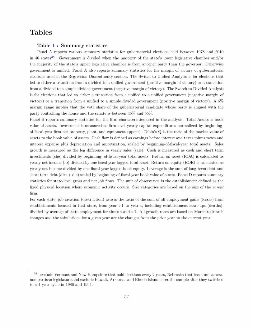
Tables

Table 1 : Summary statisticsPanel A reports various summary statistics for gubernatorial elections held between 1978 and 2010

in 46 states38. Government is divided when the majority of the state’s lower legislative chamber and/orthe majority of the state’s upper legislative chamber is from another party than the governor. Otherwisegovernment is unified. Panel A also reports summary statistics for the margin of victory of gubernatorialelections used in the Regression Discontinuity section. The Switch to Unified Analysis is for elections thatled to either a transition from a divided to a unified government (positive margin of victory) or a transitionfrom a divided to a simple divided government (negative margin of victory). The Switch to Divided Analysisis for elections that led to either a transition from a unified to a unified government (negative margin ofvictory) or a transition from a unified to a simple divided government (positive margin of victory). A 5%margin range implies that the vote share of the gubernatorial candidate whose party is aligned with theparty controlling the house and the senate is between 45% and 55%.Panel B reports summary statistics for the firm characteristics used in the analysis. Total Assets is bookvalue of assets. Investment is measured as firm-level yearly capital expenditures normalized by beginning-of-fiscal-year firm net property, plant, and equipment (ppent). Tobin’s Q is the ratio of the market value ofassets to the book value of assets. Cash flow is defined as earnings before interest and taxes minus taxes andinterest expense plus depreciation and amortization, scaled by beginning-of-fiscal-year total assets. Salesgrowth is measured as the log difference in yearly sales (sale). Cash is measured as cash and short terminvestments (che) divided by beginning- of-fiscal-year total assets. Return on asset (ROA) is calculated asyearly net income (ib) divided by one fiscal year lagged total asset. Return on equity (ROE) is calculated asyearly net income divided by one fiscal year lagged book equity. Leverage is the sum of long term debt andshort term debt (dltt + dlc) scaled by beginning-of-fiscal-year book value of assets. Panel D reports summarystatistics for state-level gross and net job flows. The unit of observation is the establishment defined as thefixed physical location where economic activity occurs. Size categories are based on the size of the parentfirm.For each state, job creation (destruction) rate is the ratio of the sum of all employment gains (losses) fromestablishments located in that state, from year t-1 to year t, including establishment start-ups (deaths),divided by average of state employment for times t and t-1. All growth rates are based on March-to-Marchchanges and the tabulations for a given year are the changes from the prior year to the current year.

38I exclude Vermont and New Hampshire that hold elections every 2 years, Nebraska that has a unicameralnon partisan legislature and exclude Hawaii. Arkansas and Rhode Island enter the sample after they switchedto a 4-year cycle in 1986 and 1994.

57

Table 1: Summary statistics

PANEL A Election Characteristics (Post Election Year)In Nber and Pct of Gubernatorial Elections Total N Pct Std.DChange from divided to unified 358 53 0.148 0.356Change from unified to divided 358 46 0.128 0.335Republican Gov. Elected 358 170 0.475 0.501Change in Gov.Party 358 116 0.324 0.472Non incumbent Gov.elected 358 191 0.534 0.498Switch to unified Analysis (used in RD)Includes "divided to divided" and "divided to unified" elections N Mean Median Std.D.Margin of Victory in pctage 133 -0.09 0.39 9.36Margin within 5% 55 0.49 0.39 2.85Switch to divided Analysis (used in RD)Includes "unified to unified" and "unified to divided" elections N Mean Median Std.D.Margin of Victory in pctage 135 -5.29 -4.30 9.60Margin within 5% 60 0.27 0.35 2.90

PANEL B Firm CharacteristicsN obs Mean Median Std.D

Investment Rate (CapExt/PPEt−1) 66,368 0.246 0.202 0.178Market-to-book 66,368 1.566 1.229 1.114Firm size (total assets,$m) 66,368 2,066 175 13,222Cash Flow 66,368 0.081 0.095 0.131Sales Growth 66,368 0.065 0.071 0.226Cash 66,368 0.140 0.068 0.189ROE 66,368 0.057 0.098 0.286ROA 66,368 0.029 0.047 0.128Leverage 66,368 0.243 0.210 0.238State-level characteristicsReal GSP growth rate 66,368 0.023 0.026 0.031

PANEL C Mean Investment Rate in Post Election YearSwitch to unified vs. No Switch N obs Mean Median Std.DT1×DU = 1 2,721 0.233 0.192 0.173T1×Switch = 0 11,669 0.251 0.206 0.180Diff(p-val clust.) 0.000Switch to divided vs. No Switch N obs Mean Median Std.DT1×UD = 1 2,806 0.247 0.201 0.181T1×Switch = 0 11,669 0.251 0.206 0.180Diff(p-val clust.) 0.005

PANEL D Employment Flows - State-level x Size statisticsN obs Mean Median Std.D

Job Creation Rate 18,480 17.57 15.80 7.68Job Destruction Rate 18,480 15.29 15.20 4.60Net Job Creation Rate 18,480 2.28 1.50 6.87N firms 18,480 8,325 808 23,089N Establishments 18,480 10,231 3.185 23,039

58

Table 2: Checks and balances and corporate investment.1978-2010.

(1) (2) (3) (4) (5) (6) (7) (8)Baseline Lagged Inv 1978-2006 Ex Presidt Divided

T1×Switch to U -0.009∗∗∗ -0.009∗∗∗ -0.009∗∗∗ -0.008∗∗ -0.009∗∗∗ -0.009∗∗∗ -0.008∗∗∗ -0.006∗∗

(0.003) (0.003) (0.003) (0.003) (0.003) (0.003) (0.003) (0.003)T1×Switch to D -0.001 -0.001 -0.000 0.000 -0.000 -0.001 -0.000 0.001

(0.004) (0.003) (0.003) (0.003) (0.003) (0.003) (0.004) (0.003)T1×U to U 0.001

(0.003)T1 (Post Election) 0.003∗∗ 0.003∗ 0.003∗ 0.002 0.003∗∗ 0.003∗ 0.000 0.003∗

(0.001) (0.002) (0.002) (0.002) (0.002) (0.002) (0.001) (0.002)TobinQ_t-1 0.046∗∗∗ 0.046∗∗∗ 0.046∗∗∗ 0.039∗∗∗ 0.046∗∗∗ 0.046∗∗∗ 0.039∗∗∗

(0.002) (0.002) (0.002) (0.002) (0.002) (0.002) (0.002)CashFlows_t 0.038∗∗∗ 0.038∗∗∗ 0.038∗∗∗ 0.037∗∗∗ 0.041∗∗∗ 0.037∗∗∗ 0.037∗∗∗

(0.004) (0.004) (0.004) (0.003) (0.004) (0.003) (0.003)Sales growth_t-1 0.016∗∗∗ 0.016∗∗∗ 0.016∗∗∗ 0.009∗∗∗ 0.015∗∗∗ 0.015∗∗∗ 0.009∗∗∗

(0.001) (0.001) (0.001) (0.001) (0.001) (0.001) (0.001)Size_t-1 -0.046∗∗∗ -0.046∗∗∗ -0.046∗∗∗ -0.053∗∗∗ -0.049∗∗∗ -0.044∗∗∗ -0.053∗∗∗

(0.005) (0.005) (0.005) (0.004) (0.005) (0.005) (0.004)Republican gov. 0.001 0.001 0.001 0.002 0.000 0.000

(0.002) (0.002) (0.002) (0.003) (0.002) (0.002)∆GSP_t− 1 0.006∗∗∗ 0.006∗∗∗ 0.005∗∗∗ 0.006∗∗∗ 0.006∗∗∗ 0.005∗∗∗

(0.002) (0.002) (0.001) (0.002) (0.002) (0.001)

Firm FE yes yes yes yes yes yes yes yesRegion x year FE yes yes yes yes yes yes yes yesInd x year FE yes yes yes yes yes yes yes yesState clusters 46 46 46 46 46 46 37 46Observations 66,368 66,368 66,368 66,368 66,352 59,308 64,224 66,352R2 0.40 0.45 0.45 0.45 0.47 0.45 0.46 0.47

Note: This table presents estimates from regressions of the type:INVist = Firmi + Industryjt + β1 T1st + β2 T1st × Ust + β3 T1st ×Dst + Γ′Xist−1 + Λ′Wst−1 +RegionRt + εist.i indexes firm, s state, j industry (Fama French 48 industry classification), R census region and t year. The dependent variable is CapExist/PPEist−1. T1 is anindicator variable set to one in the post-election year. The "Switch to U" ("Switch to D") indicator variable is set to one when a state transitions from divided to unified(from unified to divided). Xist is a vector of firm characteristics: Tobin’s Q, cash flows, size, yearly sales’ growth. Wst is a vector of state controls including an indicatorvariable for the governor party and the percentage change in real gross state product over the previous year. All continuous independent variables are standardized.Firmi, Industryjt and RegionRt are firm, industry x year and census region x year fixed effects. Time period spans 1978-2010 in all but col. 6. In col. 7, I drop thestates which have gubernatorial elections concurrent with presidential elections. In col. 8 I use a broader definition of divided government: a government is dividedwhen all three institutions of state government are not controlled by the same party, even if there are not enough legislators to override a gubernatorial veto. Robuststandard errors are clustered by state and reported in brackets. *, ** and *** indicate statistical significance at the 10%, 5% and 1% level.

59

Table 3: Corporate investment dynamics around changes in checks and balances. 1978-2010.

T0=Election T1=PostElection T2 All(1) (2) (3) (4)

T0×Switch to U 0.003 0.002(0.003) (0.003)

T1×Switch to U -0.009∗∗∗ -0.009∗∗

(0.003) (0.003)

T2×Switch to U 0.002 0.001(0.002) (0.002)

T0×Switch to D -0.001 -0.002(0.004) (0.004)

T1×Switch to D -0.000 -0.000(0.003) (0.004)

T2×Switch to D 0.000 0.000(0.003) (0.003)

Firm cov. Tobin_Q, CF Tobin_Q, CF Tobin_Q, CF Tobin_Q, CF- ∆Sales, Size ∆Sales, Size ∆Sales, Size ∆Sales, SizeState cov. Gov, ∆gsp Gov, ∆gsp Gov, ∆gsp Gov, ∆gsp- T0 T1 T2 T0,T1,T2Firm FE yes yes yes yesInd x year FE yes yes yes yesRegion x year FE yes yes yes yesState clusters 46 46 46 46Observations 66,368 66,368 66,368 66,368R2 0.45 0.45 0.45 0.45Test for linear combination -T1×Switch to U + T2× Switch to U -0.003t_stat -1.22

Note: This table presents estimates from equation (2) over the period 1978-2010 (column 4). The dependent variable is

CapExist/PPEist−1. Tks is an indicator variable equal to 1 in state s in year k. k=0 in the election year. k=1 in the

post-election year and k=2 in the second year after an election. T1×Switch to U is set to 1 when government transitions from

divided to unified. T0×Switch to U (T2×Switch to U) is the 1-year lag (lead) of T1×Switch to U. T1×Switch to D is set to 1

when government transitions from unified to divided. T0×Switch to D (T2×Switch to D) is the 1-year lag (lead) of T1×Switch

to D. Firm-level controls include Tobin’s Q, cash flows, size and sales growth. State-level controls include the party of the

elected governor and growth in state real gsp. All continuous independent variables are standardized. Robust standard errors

are clustered by state. Associated t-statistics are reported in brackets. *, ** and *** indicate statistical significance at the

10%, 5% and 1% level, respectively.

60

Table 4: Regression Discontinuity

Switch to Unified Switch to Divided

MSE-Opt MSE-Opt CER-opt Placebo in T0 MSE-Opt MSE-Opt

Coef.(robust) -0.009∗∗ -0.009∗∗ -0.011∗∗ 0.004 0.003 0.004[0.004] [0.004] [0.005] [0.004] [0.004] [0.004]

N obs. 2,484 2,320 1,601 2,712 3,152 2,824Bandwidth 4.7 4.9 3.1 5.4 4.4 4.0Covariates yes yes yesN elections 52 53 33 57 51 49N elections right 28 28 14 31 26 26

Note: This table presents estimates from investment regressions of the type :

INVis = α+ β Zs + f(Vs) + Γ′Xi + εi

f(Vs) = b1V + b2V × Zs

INVis is the investment rate of firm i, headquartered in state s, after absorbing firm fixed effects, defined as CapExist/TAist−1.

Vs is the margin of winning or losing (ahead of 50%) in the gubernatorial election in state s in year t-1. In columns 1 to 3

the sample is limited to post-election years, for states that were ex-ante divided and that either stayed divided or switched to

unified. If V is above 0 the state becomes unified. If V is below 0 the state stays divided. In column 4 the sample is limited to

election years for the same set of states. In columns 5 and 6 the sample is limited to post-election years, for states that were

ex-ante unified and that either stayed unified or switched to divided. If V is above 0 the state becomes divided. If V is below 0

the state stays unified. Z is an indicator equal to 1 if Vs >= 0 and 0 otherwise. X is a vector of pre-determined control variables

including Tobin’s Q and cash flows. f(.) is a first-order polynomial function, approximated through a triangular kernel-weighted

local linear regression. All columns but column 3 report results for estimations within one common MSE-optimal bandwidth,

chosen by Calonico, Cattaneo, and Titiunik (2014) procedure ; column 3 reports results for estimations within one common

CER-optimal bandwidth, chosen by Calonico, Cattaneo, and Titiunik (2014) procedure. A 5% margin of victory implies that

the vote share of the gubernatorial candidate is between 45% and 55%. I report robust standard errors estimates from Calonico,

Cattaneo, and Titiunik (2014). Associated t-statistics are reported in brackets. *, ** and *** indicate statistical significance

at the 10%, 5% and 1% level, respectively.

61

Table 5: Checks and balances and investment sensitivity to state-level exposure.

1978-2010 1993-2008

(1) (2) (3) (4)HQ state HQ state HQ state = 10K state HQ state = 10K state

T1×Switch to U×Small -0.016∗ -0.030∗∗

(0.009) (0.014)T1×Switch to D×Small -0.000 -0.019

(0.008) (0.019)T1×Switch to U -0.006 -0.005 -0.009∗ -0.001

(0.004) (0.004) (0.005) (0.006)T1×Switch to D 0.002 -0.001 0.004 0.009∗∗

(0.003) (0.004) (0.004) (0.004)T1×Small -0.000 0.005

(0.003) (0.007)T1 (Post Election) 0.003∗∗ 0.004 0.007∗∗ 0.005∗

(0.002) (0.002) (0.003) (0.003)

Firm, State cov. yes yes yes yesFirm, Ind x year yes yes yes yesRegion x year yes yes yes yesState clusters 46 45 43 43Observations 66,368 25,005 16,395 16,395R2 0.45 0.52 0.55 0.54

Note: This table presents estimates of the type :

INVist = Firmi + β2 T1st × Ust + β3 T1st ×Dst + γ2 T1st × Ust × Smallit + γ2 T1st ×Dst × Smallit

+ γ0 T1st × Smallit + β1 T1st + Γ′Xist−1 + Λ′Wst−1 + Industryjt +RegionRt + εist

over the period 1978-2010 (column 1) and 1993-2008 (columns 2 to 4). The dependent variable is CapExist/PPEist−1. T1 is

an indicator variable equal to 1 in the post-election year. SwitchtoU is set to 1 when government transitions from divided to

unified. SwitchtoD is set to 1 when government transitions from unified to divided. Small is an indicator equal to one for firms

in the bottom quartile of size distribution in year t. Firm location is based solely on its headquarter state in columns 1 and

2, and on both its headquarter and its operation states in columns 3 and 4. In columns 3 and 4 I restrict the sample to firms

for which headquarter state is identical to operation state (most frequently mentioned state in a firm annual 10-K filings using

García and Norli (2012) dataset). Firm-level controls include Tobin’s Q, cash flows, size and sales growth. State-level controls

include the party of the elected governor and growth in state real gsp. All continuous independent variables are standardized.

Robust standard errors are clustered by state. Associated t-statistics are reported in brackets. *, ** and *** indicate statistical

significance at the 10%, 5% and 1% level, respectively.

62

Table 6: Checks and balances and corporate investment conditional on political polarization

Republican Revolution State Legislative Polarization

(1) (2) (3)1978-1993 1994-2010

T1×Switch to U×HighPol -0.004(0.005)

T1×Switch to D×HighPol -0.011∗∗

(0.005)T1×Switch to U -0.010∗∗ -0.010∗∗ -0.008∗∗

(0.005) (0.004) (0.004)T1×Switch to D 0.006 -0.007∗ 0.003

(0.005) (0.004) (0.003)T1×HighPol 0.009∗∗∗

(0.002)T1 (Post Election) 0.000 0.006∗∗∗ 0.001

(0.002) (0.002) (0.002)

Firm, State cov. yes yes yesFirm, Ind x year FE yes yes yesRegion x year FE yes yes yesState clusters 45 46 46Observations 30,722 35,395 66,368R2 0.46 0.52 0.45

Note: This table presents estimates of equation (1) in columns 1 and 2 and estimates of equation (3) below in column 3 :

INVist = Firmi + β2 T1st × Ust + β3 T1st ×Dst + γ2 T1st × Ust ×HighPolst + γ2 T1st ×Dst ×HighPolst

+ γ0 T1st ×HighPolst + β1 T1st + Γ′Xist−1 + Λ′Wst−1 + Industryjt +RegionRt + εist(3)

The dependent variable is CapExist/PPEist−1. T1 is an indicator variable equal to 1 in the post-election year. SwitchtoU

is set to 1 when government transitions from divided to unified. SwitchtoD is set to 1 when government transitions from

unified to divided. The High Polarization indicator HighPol is set to one when a state is in the Top 10 of state-level legislative

polarisation, based on Shor and McCarty (2011) (column 3). Firm-level controls include Tobin’s Q, cash flows, size and sales

growth. State-level controls include the party of the elected governor and growth in state real gsp. All continuous independent

variables are standardized. Robust standard errors are clustered by state. Associated t-statistics are reported in brackets. *,

** and *** indicate statistical significance at the 10%, 5% and 1% level, respectively.

63

Table 7: Checks and balances and corporate employment

All firms Less than 2,500 employees

(1) (2) (3) (4)Job creation Job destruction Job creation Job destruction

T1×Switch to U -0.253∗ -0.082 -0.315∗∗ -0.076(0.127) (0.151) (0.132) (0.167)

T1×Switch to D 0.326∗ -0.026 0.245 0.035(0.194) (0.137) (0.244) (0.148)

T1 (Post Election) 0.031 0.021 0.046 -0.005(0.068) (0.080) (0.069) (0.087)

State cov. yes yes yes yesSize FE Yes Yes Yes YesState FE Yes Yes Yes YesRegion x year FE Yes Yes Yes YesState clusters 46 46 46 46Observations 18,480 18,480 13,860 13,860R2 0.80 0.52 0.84 0.64

This table presents estimates from regressions of the type :

Jobkst = +β1 T1s,t + β2 T1st ×Ust + β3 T1st ×Dst + γ1 ∆RealGSP/capitas,t−2 + γ2 StatePopulations,t−2 + c0 Republicanst

+ Sizek + States +RegionRt + εkst

s indexes the state of the establishment, k the size of the parent firm, R Census region and t denotes time. The main dependent

variable is the establishment JCRs,t, the job creation rate in state s between year t and year t-1, in percentages. For each

state, JCRs,t is the ratio of the sum of all employment gains from expanding establishments from year t-1 to year t - including

establishment startups - divided by average of state employment for times t and t-1. %change real GSP/capita is the percentage

change in real gross state product per capita for a given state from year t-2 to and t-1. As employment rates are reported as

of March 12th of each year in the BDS, a gubernatorial election occurring on November of year t is matched with changes in

employment from March t to March t+1. The post-election dummy (T1) is defined relative to the election year as T0 + 1

year.Robust standard errors are clustered by state and reported in brackets. *, ** and *** indicate statistical significance at

the 10%, 5% and 1% level, respectively.

64

Table 8: Checks and balances and return volatility

Investment Realized volatility

(1) (2) (3) (4) (5)

T1×Switch to U×Small 0.013∗

(0.007)T1×Switch to D×Small -0.006

(0.004)T1×Switch to U -0.008∗∗ 0.004∗∗ 0.004∗∗ 0.004∗∗ 0.001

(0.003) (0.002) (0.002) (0.002) (0.002)T1×Switch to D -0.004 -0.001 -0.001 -0.002 -0.000

(0.003) (0.002) (0.002) (0.002) (0.002)T1 (Post Election) 0.001 0.001 0.001 0.000 -0.000

(0.002) (0.001) (0.001) (0.001) (0.001)T1×New governor 0.004∗

(0.002)T1×Small 0.006∗∗∗

(0.002)

Firm cov. yes yes yes yesState cov. yes yes yes yes- yes New govFirm, Ind x year FE yes yes yes yes yesRegion x year FE yes yes yes yes yesState clusters 46 46 46 46 46Observations 61,016 61,016 61,016 61,016 61,016R2 0.47 0.50 0.51 0.50 0.51

This table presents estimates from regressions of the type: This table presents estimates from regressions of the type:

Yist = +β2 T1st × Ust + β3 T1st ×Dst + γ2 T1st × Ust × Smalli + γ2 T1st ×Dst × Smallist + γ0 T1st × Smalli + β1 T1st

+ Γ′Xist−1 + Λ′Wst−1 + Firmi + Industryjt +RegionRt + εist

i indexes firm, s state, j industry (Fama French 48 industry classification), R census region and t time (calendar year). In

column 1 the dependent variable Y is the investment rate as defined previously. In columns 2 to 5, the dependent variable is

the standard deviation of firm monthly stock returns (adjusted for dividends) over a calendar year, winsorized to be between

0 and 200% as in Stein and Stone (2013). T1 is the post-election year dummy. The "Switch to Unified" dummy (U) is set to

1 when a state transitions from divided to unified. The "Switch to Divided" dummy (D) is set to 1 when a state transitions

from unified to divided. New governor is an indicator variable taking the value one when a non incumbent governor is elected.

Small is an indicator variable set to one for firms in the bottom quartile of the size distribution. Xist−1 is a vector of firm

characteristics (Tobin’s Q, cash flows, size and sales growth).Wst−1 is a vector of state controls (party of the elected governor,

real gsp growth). All continuous independent variables are standardized to facilitate economic interpretation. Robust standard

errors are clustered by state and reported in brackets. *, ** and *** indicate statistical significance at the 10%, 5% and 1%

level, respectively.

65

Table 9: Checks and balances, investment and the policy uncertainty channel

Baseline 1984-2010 I =1 if Low redeployability I =1 if Durable good industry

All All Small All Small

T1×Switch to U×I -0.031∗ -0.039∗∗ -0.024∗∗ -0.044∗∗∗

(0.016) (0.018) (0.011) (0.010)T1×Switch to D×I -0.014 -0.011 -0.012 -0.019

(0.013) (0.015) (0.012) (0.016)T1×Switch to U -0.017∗∗∗ -0.013∗∗ -0.016∗∗ -0.008∗∗ -0.010∗∗∗

(0.005) (0.006) (0.007) (0.003) (0.003)T1×Switch to D -0.008 -0.008 -0.009 0.000 -0.001

(0.007) (0.006) (0.009) (0.003) (0.005)T1×I -0.010 -0.014 0.003 0.009

(0.008) (0.009) (0.008) (0.009)T1 (Post Election) 0.009∗∗∗ 0.011∗∗∗ 0.010∗∗∗ 0.003∗ 0.005∗∗

(0.002) (0.002) (0.002) (0.001) (0.002)

Firm, state cov. yes yes yes yes yesFirm, Ind x year FE yes yes yes yes yesRegion x year FE yes yes yes yes yesState clusters 45 45 45 46 46Observations 29,515 29,500 21,545 66,408 49,599R2 0.49 0.50 0.47 0.45 0.44

This table presents estimates from regressions of the type:

INVist = γ2 T1st × Ust × I + γ2 T1st × Ust × I + β2 T1st ×Dst + β3 T1st ×Dst

+ γ0 T1st × I + β1 T1st + Γ′Xist−1 + Λ′Wst−1 + Firmi + Industryjt +RegionRt + εist

i indexes firm, s state, j industry (Fama French 48 industry classification), R census region and t time (calendar year). The

dependent variable is the investment rate defined as CapExist/PPEist−1. T1 is an indicator variable set to one in the post-

election year. Switch to unified dummy (U) takes the value one when government transitions from divided to unified. Switch

to divided (D) takes the value one when government transitions from unified to divided. I use firm-level measures of asset

redeployability from Kim and Kung, 2016. Column 1 reports baseline results for the sub-sample of firms for which this data

is available. The indicator variable I is set to one when a firm has a low asset redeployability score (bottom quartile of the

annual distribution) (col. 2 and 3) ; when a firm operates in a durable goods industry (col. 4 and 5). In columns 3 and 5 the

sample is limited to smaller firms - firms below the 75th percentile of the size distribution - to measure the degree of geographic

concentration as a proxy for a higher exposure to local state policy. Xist−1 is a vector of firm characteristics (Tobin’s Q, cash

flows, size and sales growth).Wst−1 is a vector of state controls (party of the elected governor, real gsp growth). All continuous

independent variables are standardized to facilitate economic interpretation. Robust standard errors are clustered by state and

reported in brackets. *, ** and *** indicate statistical significance at the 10%, 5% and 1% level, respectively.

66

Appendix A. Supplementary tables

67

Table A1: Variable definitionsFirm Variables Definition SourceInvestment Rate Capital Expenditures t (PPENT) Compustat

divided by Total Assets t-1 (AT)Firm Size Logarithm of total assets (AT) ComputstatSales growth Log difference in annual sales (SALE) CompustatCash holdings Cash and short term investments t (CHE) Compustat

divided by Total Assets t-1Market-to-book Book assets minus book equity Compustat

(SEQ (*) + TXDITC - PSTK) plus market equity(PRCC×CSHO) all divided by book assets(*) If missing I take CEQ-PSTK or AT-LT

Cash Flow Income before extraordinary items t (IBC) Compustatdivided by total assets t-1

Leverage Long-term debt plus short-term debt Compustat(DLTT + DLC) divided by total assets t-1

ROA Earnings before extraordinary items t (IB) Compustatdivided by total assets t-1

ROE Earnings before extraordinary items t (IB) Compustatdivided by book value of equity t-1

State Election Variables Definition SourceDivided government All three institutions of state government Klarner, 2013c

(two chambers and governor’s office)are not controlled by the same partyand there are not enough legislatorsto override a gubernatorial veto

Unified government Government is not divided Klarner, 2013cSwitch to Divided Dummy variable that takes the value of one

if the gubernatorial election leads toa change from a unified to a divided state

Switch to Unified Dummy variable that takes the value of oneif the gubernatorial election leads toa change from a divided to a unified state

Republican governor Dummy set to one during all years served by Klarner, 2013aa Republican governor

New Dummy set to one when the elected governor Klarner, 2013ais not an incumbent

High Polarization Dummy set to one when a state is in the Top 10 Shor and McCarty, 2011of state-level legislative polarisation

Election Margin Difference in the percentage of votes received by List and Sturm, 2006,the winning candidate and by her opponent Congressional Quarterly

PAI The political alignment index (PAI) is computed by Klarner, 2013c0.25×Governor +0.25× Senators + 0.25×Representatives Kim, Pantzalis, and Park, 2012+ 0.25×[0.5×State senators + 0.5×State representatives]Governor is a dummy set to one if the governor is in thesame party as the President. Senators, rep., state sen.and state rep. are dummy set to one if, thepercent of members in the President’s party is greaterthan 50%.

State Economic Variables Definition SourceGSP State Real GDP growth Klarner, 2013bUnemployment State unemployment rate Bureau of Labor StatisticsState Budget Surplus Budget General Revenue - General Expenditure Klarner, 2013b

as a percent of gross state product (GSP)State Debt Outstanding Total Debt Outstanding over GSP Klarner, 2013bState Tax Revenue Tax Revenue over GSP Klarner, 2013b

68

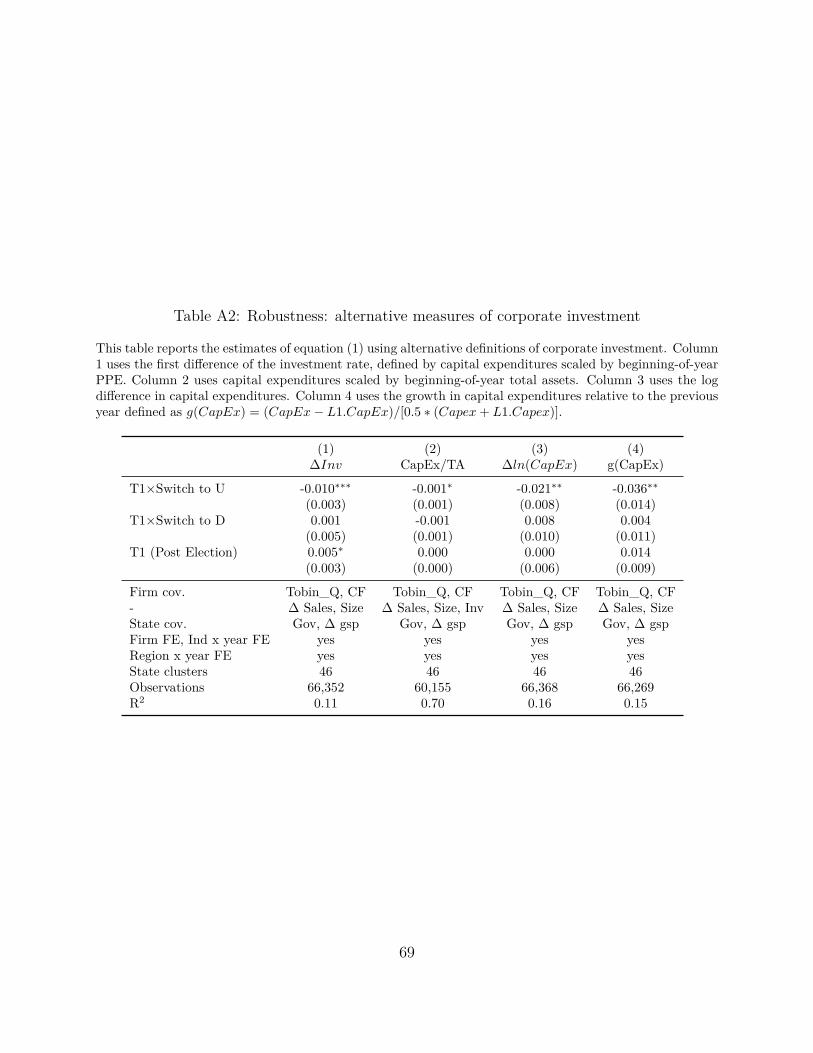
Table A2: Robustness: alternative measures of corporate investment

This table reports the estimates of equation (1) using alternative definitions of corporate investment. Column1 uses the first difference of the investment rate, defined by capital expenditures scaled by beginning-of-yearPPE. Column 2 uses capital expenditures scaled by beginning-of-year total assets. Column 3 uses the logdifference in capital expenditures. Column 4 uses the growth in capital expenditures relative to the previousyear defined as g(CapEx) = (CapEx− L1.CapEx)/[0.5 ∗ (Capex+ L1.Capex)].

(1) (2) (3) (4)∆Inv CapEx/TA ∆ln(CapEx) g(CapEx)

T1×Switch to U -0.010∗∗∗ -0.001∗ -0.021∗∗ -0.036∗∗

(0.003) (0.001) (0.008) (0.014)T1×Switch to D 0.001 -0.001 0.008 0.004

(0.005) (0.001) (0.010) (0.011)T1 (Post Election) 0.005∗ 0.000 0.000 0.014

(0.003) (0.000) (0.006) (0.009)

Firm cov. Tobin_Q, CF Tobin_Q, CF Tobin_Q, CF Tobin_Q, CF- ∆ Sales, Size ∆ Sales, Size, Inv ∆ Sales, Size ∆ Sales, SizeState cov. Gov, ∆ gsp Gov, ∆ gsp Gov, ∆ gsp Gov, ∆ gspFirm FE, Ind x year FE yes yes yes yesRegion x year FE yes yes yes yesState clusters 46 46 46 46Observations 66,352 60,155 66,368 66,269R2 0.11 0.70 0.16 0.15

69

Table A3: Robustness: Post-election year definitionThis table reports the estimates of equation (1) using alternative definitions of the post election year T1.Definition 1: The post-election dummy variable takes a value of one for any firm-year in which an electionis held no later than 1 months after the fiscal year beginning in year t.Definition 2: The post-election dummy variable takes a value of one for any firm-year in which an electionis held no later than 3 months after the fiscal year beginning in year t.Definition 3: The post-election dummy variable takes a value of one for any firm-year in which an electionis held no later than 4 months after the fiscal year beginning in year t.

(1) (2) (3)Definition 1 Definition 2 Definition 3

T1×Switch to U -0.009∗∗∗ -0.008∗∗∗ -0.007∗∗∗

(0.003) (0.003) (0.003)T1×Switch to D 0.001 -0.000 -0.002

(0.003) (0.003) (0.003)T1 (Post Election) 0.002 0.001 0.001

(0.002) (0.002) (0.002)

Firm cov. Tobin_Q, CF Tobin_Q, CF Tobin_Q, CF- ∆ Sales, Size ∆ Sales, Size ∆ Sales, SizeState cov. Gov, ∆ gsp Gov, ∆ gsp Gov, ∆ gspFirm FE, Ind x year FE yes yes yesRegion x year FE yes yes yesState clusters 46 46 46Observations 66,368 66,368 66,368R2 0.45 0.45 0.45

70

Table A4: Additional state-level control variables

This table presents estimates from equation (1) augmented by additional state controls (Wst) : 1) changein the state employment rate, 2) change in state tax revenue (as a percentage of GSP), 3) change in statebudget surplus, 4) change in state debt outstanding. Only the parameters of interest are reported.

(1) (2) (3) (4)Unemployment Tax Revenues Budget Deficit Debt Outstanding

T1×Switch to U -0.009∗∗∗ -0.009∗∗∗ -0.008∗∗∗ -0.009∗∗∗

(0.003) (0.003) (0.003) (0.003)T1×Switch to D 0.000 -0.000 -0.000 -0.000

(0.003) (0.003) (0.003) (0.003)T1 (Post Election) 0.003∗ 0.003∗ 0.003∗ 0.003∗

(0.002) (0.002) (0.002) (0.002)∆Unempt−1 -0.003∗∗∗

(0.001)∆Taxt−1 0.001

(0.001)∆Budgett−1 0.001

(0.001)∆Debtt−1 0.000

(0.001)

Firm cov. Tobin_Q, CF Tobin_Q, CF Tobin_Q, CF Tobin_Q, CF- ∆ Sales, Size ∆ Sales, Size ∆ Sales, Size ∆ Sales, SizeState cov. Gov, ∆ gsp Gov, ∆ gsp Gov, ∆ gsp Gov, ∆ gspFirm FE, Ind x year FE yes yes yes yesRegion x year FE yes yes yes yesState clusters 46 46 46 46Observations 66,368 66,368 66,368 66,368R2 0.45 0.45 0.45 0.45

71

Table A5: Additional firm control variables

This table presents estimates from equation (1) augmented by additional firm controls (Xist) : 1) leverage(short-term and long-term debt scaled by total assets), 2) tangibility (Net PPE over total assets), 3) cashholdings (cash and short-term investments scaled by total assets), 4) age of the firm (ln(age) and ln(age)2).Only the parameters of interest are reported.

(1) (2) (3) (4) (5)Leverage PP&E ratio Cash Age -

T1×Switch to U -0.010∗∗∗ -0.007∗∗∗ -0.008∗∗∗ -0.009∗∗∗ -0.009∗∗∗

(0.003) (0.002) (0.003) (0.003) (0.003)T1×Switch to D 0.001 0.000 0.001 -0.000 -0.000

(0.003) (0.003) (0.003) (0.003) (0.003)Leverage t-1 -0.021∗∗∗

(0.001)PP&E/TA t-1 -0.070∗∗∗

(0.006)Cash 0.032∗∗∗

(0.001)Age 0.003 -0.012

(0.005) (0.034)Age2 0.004

(0.009)

Firm cov. Tobin_Q, CF Tobin_Q, CF Tobin_Q, CF Tobin_Q, CF Tobin_Q, CF- ∆ Sales, Size ∆ Sales, Size ∆ Sales, Size ∆ Sales, Size ∆ Sales, SizeState cov. Gov, ∆ gsp Gov, ∆ gsp Gov, ∆ gsp Gov, ∆ gsp Gov, ∆ gspFirm FE, Ind x year FE yes yes yes yes yesRegion x year FE yes yes yes yes yesState clusters 46 46 46 46 46Observations 59,999 60,155 60,149 66,352 66,352R2 0.49 0.50 0.50 0.47 0.47

72

Table A6: Alignment with presidential party, Southern states, partisanship, incumbency

I=1 if High PAI I=1 if Low PAI I=1 if South I=1 if Rep.gov I=1 if NonIncumbent

(1) (2) (3) (4) (5) (6)

T1×Switch to U -0.010∗∗∗ -0.008∗∗∗ -0.007∗ -0.010∗∗

(0.003) (0.003) (0.004) (0.005)T1×Switch to D -0.001 -0.001 0.005 0.002

(0.004) (0.004) (0.005) (0.005)T1×Switch to U×I 0.003 -0.004 -0.004 0.002

(0.008) (0.005) (0.007) (0.007)T1×Switch to D×I 0.004 0.009 -0.006 -0.003

(0.005) (0.008) (0.005) (0.007)T1×I 0.003 -0.002 0.001 0.004 0.005∗ -0.000

(0.003) (0.003) (0.004) (0.002) (0.003) (0.002)T1 (Post Election) 0.003 0.003 0.003 0.001 -0.000 0.004∗

(0.002) (0.002) (0.002) (0.002) (0.002) (0.002)I 0.006∗ -0.003

(0.003) (0.003)

Firm cov. Tobin_Q, CF Tobin_Q, CF Tobin_Q, CF Tobin_Q, CF Tobin_Q, CF Tobin_Q, CF- ∆ Sales, Size ∆ Sales, Size ∆ Sales, Size ∆ Sales, Size ∆ Sales, Size ∆ Sales, SizeState cov. Gov, ∆ gsp Gov, ∆ gsp Gov, ∆ gsp Gov, ∆ gsp Gov, ∆ gsp Gov, ∆ gspFirm FE, Ind x year FE yes yes yes yes yes yesRegion x year FE yes yes yes yes yes yesState clusters 46 46 46 46 46 46Observations 66,368 66,368 66,368 66,368 66,368 66,368R2 0.47 0.47 0.47 0.47 0.47 0.47

Note : This table presents estimates from regressions of the type:INVist = Firmi + γ1 T1st×Dst× Ist + γ2 T1st×Ust× Ist + β1 T1st + β2 T1st×Ust + β3 T1st×Dst + γ3 T1st× Ist + γ4 Ist + Γ′Xist−1 + Λ′Wst−1 +RegionRt + εist.

i indexes firm, s state, j industry (Fama French 48 industry classification), R census region and t year. The dependent variable is CapExist/PPEist−1. T1 is anindicator variable set to one in the post-election year. Ust (Dst) is an indicator variable set to one when a state transitions from divided to unified (from unified todivided). Ist is a dummy set to one when 1) the state political alignment with the presidential party is high (political alignment index in the top quartile) (col.1),2) the state political alignment with the presidential party is low (political alignment index in the bottom quartile (col.2), 3) the state belongs to the Census Southregion (DE,FL,GE,MD,NC,SC,VI,WV,AL,KT,MS,TN,AR,LA,OK,TX) (col.3), 4) the elected governor is a Republican (col.4 and 5), 5) the elected governor is not anincumbent (col.6). Xist is a vector of firm controls. Wst is a vector of state controls. All continuous independent variables are standardized. Firmi, Industryjt andRegionRt are firm, industry x year and census region x year fixed effects. Time period spans 1978-2010. Robust standard errors are clustered by state and reported inbrackets. *, ** and *** indicate statistical significance at the 10%, 5% and 1% level.

73

Table A7: Balanced covariates test

This table presents estimates from regressions of the type : Xis = α + β Zs + f(Vs) + εi. Xis is acharacteristic of firm i, headquartered in state s, in election year i.e. in t-1, before the switch. Vs isthe margin of winning or losing (ahead of 50%) in the gubernatorial election in state s in year t-1. Incolumns 1 and 2 (resp. 3 and 4) the sample is limited to post-election years, for states that were ex-antedivided (unified) and that, either stayed divided (unified), or switched to divided. If V is above 0 the statebecomes unified (divided). If V is below 0 the state stays divided (unified). f(.) is a first-order polynomialfunction, approximated through a triangular kernel-weighted local linear regression. For each characteristic,the table reports results for estimations using an MSE-optimal bandwidth, defined as in Calonico et al.(2014). I report robust standard errors estimates from Calonico et al. (2014). Associated t-statistics arereported in brackets. *, ** and *** indicate statistical significance at the 10%, 5% and 1% level, respectively.

TobinQ CF TobinQ CF

Coef.(robust) -0.042 -0.041 -0.012 0.005[0.042] [0.040] [0.051] [0.042]

N obs. 2,560 2,447 2,140 1,888MSE-opt Bandwidth 6.2 5.6 4.6 4.1

74