NBER WORKING PAPER SERIES

THE RACE BETWEEN MACHINE AND MAN:IMPLICATIONS OF TECHNOLOGY FOR GROWTH, FACTOR SHARES AND EMPLOYMENT

Daron AcemogluPascual Restrepo

Working Paper 22252http://www.nber.org/papers/w22252

NATIONAL BUREAU OF ECONOMIC RESEARCH1050 Massachusetts Avenue

Cambridge, MA 02138May 2016, Revised June 2017

We thank Philippe Aghion, Mark Aguiar, David Autor, Erik Brynjolfsson, Chad Jones, John Van Reenen, and participants at various conferences and seminars for useful comments and suggestions. We gratefully acknowledge financial support from the Bradley Foundation and the Toulouse Network on Information Technology. Restrepo thanks the Cowles Foundation and the Yale Economics Department for their hospitality. The views expressed herein are those of the authors and do not necessarily reflect the views of the National Bureau of Economic Research.

NBER working papers are circulated for discussion and comment purposes. They have not been peer-reviewed or been subject to the review by the NBER Board of Directors that accompanies official NBER publications.

© 2016 by Daron Acemoglu and Pascual Restrepo. All rights reserved. Short sections of text, not to exceed two paragraphs, may be quoted without explicit permission provided that full credit, including © notice, is given to the source.

The Race Between Machine and Man: Implications of Technology for Growth, Factor Shares and EmploymentDaron Acemoglu and Pascual RestrepoNBER Working Paper No. 22252May 2016, Revised June 2017JEL No. J23,J24,O14,O31,O33

ABSTRACT

We examine the concerns that new technologies will render labor redundant in a framework in which tasks previously performed by labor can be automated and new versions of existing tasks, in which labor has a comparative advantage, can be created. In a static version where capital is fixed and technology is exogenous, automation reduces employment and the labor share, and may even reduce wages, while the creation of new tasks has the opposite effects. Our full model endogenizes capital accumulation and the direction of research towards automation and the creation of new tasks. If the long-run rental rate of capital relative to the wage is sufficiently low, the long-run equilibrium involves automation of all tasks. Otherwise, there exists a stable balanced growth path in which the two types of innovations go hand-in-hand. Stability is a consequence of the fact that automation reduces the cost of producing using labor, and thus discourages further automation and encourages the creation of new tasks. In an extension with heterogeneous skills, we show that inequality increases during transitions driven both by faster automation and introduction of new tasks, and characterize the conditions under which inequality is increasing or stable in the long run.

Daron AcemogluDepartment of Economics, E52-446MIT77 Massachusetts AvenueCambridge, MA 02139and CIFARand also NBERdaron@mit.edu

Pascual RestrepoDepartment of EconomicsBoston University270 Bay State RdBoston, MA 02215and Cowles Foundation, Yalepascual.restrepo@yale.edu

1 Introduction

The accelerated automation of tasks performed by labor raises concerns that new technologies will

make labor redundant (e.g., Brynjolfsson and McAfee, 2012, Akst, 2014, Autor, 2015). The recent

declines in the labor share in national income and the employment to population ratio in the U.S.

(e.g., Karabarbounis and Neiman, 2014, and Oberfield and Raval, 2014) are often interpreted as

supporting evidence for the claims that, as digital technologies, robotics and artificial intelligence

penetrate the economy, workers will find it increasingly difficult to compete against machines, and

their compensation will experience a relative or even absolute decline. Yet, we lack a comprehensive

framework incorporating such effects, as well as potential countervailing forces.

The need for such a framework stems not only from the importance of understanding how and

when automation will transform the labor market, but also from the fact that similar claims have

been made, but have not always come true, about previous waves of new technologies. Keynes

famously foresaw the steady increase in per capita income during the 20th century from the in-

troduction of new technologies, but incorrectly predicted that this would create widespread tech-

nological unemployment as machines replaced human labor (Keynes, 1930). In 1965, economic

historian Robert Heilbroner confidently stated that “as machines continue to invade society, du-

plicating greater and greater numbers of social tasks, it is human labor itself—at least, as we now

think of ‘labor’—that is gradually rendered redundant”(quoted in Akst, 2014). Wassily Leontief

was equally pessimistic about the implications of new machines. By drawing an analogy with the

technologies of the early 20th century that made horses redundant, in an interview he speculated

that “Labor will become less and less important. . .More and more workers will be replaced by

machines. I do not see that new industries can employ everybody who wants a job”(The New York

Times, 1983).

This paper is a first step in developing a conceptual framework to study how machines re-

place human labor and why this might (or might not) lead to lower employment and stagnant

wages. Our main conceptual innovation is to propose a unified framework in which tasks previ-

ously performed by labor are automated, while at the same time other new technologies complement

labor—specifically, in our model this takes the form of the introduction of new tasks in which labor

has a comparative advantage. Herein lies our answer to Leontief’s analogy: the difference between

human labor and horses is that humans have a comparative advantage in new and more complex

tasks. Horses did not. If this comparative advantage is sufficiently important and the creation of

new tasks continues, employment and the labor share can remain stable in the long run even in the

face of rapid automation.

The importance of these new tasks is well illustrated by the technological and organizational

changes during the Second Industrial Revolution, which not only involved the replacement of the

stagecoach by the railroad, sailboats by steamboats, and of manual dock workers by cranes, but also

the creation of new labor-intensive tasks. These tasks generated jobs for a new class of engineers,

machinists, repairmen, conductors, back-office workers and managers involved with the introduction

1

and operation of new technologies (e.g., Landes, 1969, Chandler, 1977, and Mokyr, 1990).

Today, while industrial robots, digital technologies and computer-controlled machines replace la-

bor, we are again witnessing the emergence of new tasks ranging from engineering and programming

functions to those performed by audio-visual specialists, executive assistants, data administrators

and analysts, meeting planners and computer support specialists. Indeed, during the last 30 years,

new tasks and new job titles account for a large fraction of U.S. employment growth. To document

this fact, we use data from Lin (2011) to measure the share of new job titles—in which workers per-

form newer tasks than those employed in more traditional jobs—within each occupation. In 2000,

about 70% of computer software developers (an occupation employing one million people at the

time) held new job titles. Similarly, in 1990 radiology technician and in 1980 management analyst

were new job titles. Figure 1 shows that for each decade since 1980, employment growth has been

greater in occupations with more new job titles. The regression line indicates that occupations with

10 percentage points more new job titles at the beginning of each decade grow 5.05% faster over

the next 10 years (standard error=1.3%). From 1980 to 2007, total employment in the U.S. grew

by 17.5%. About half (8.84%) of this growth is explained by the additional employment growth in

occupations with new job titles relative to a benchmark category with no new job titles.1

-200

-150

-100

-50

050

100

150

200

Per

cent

chan

ge

in e

mplo

ymen

t gro

wth

by

dec

ade

0 20 40 60 80Share of new job titles at the beginning of each decade

From 1980 to 1990 From 1990 to 2000 From 2000 to 2007

Figure 1: Employment growth by decade plotted against the share of new job titles at the beginning of each decade

for 330 occupations. Data from 1980 to 1990 (in dark blue), 1990 to 2000 (in blue) and 2000 to 2007 (in light blue,

re-scaled to a 10-year change). Data source: See Appendix B.

We start with a static model in which capital is fixed and technology is exogenous. There are

two types of technological changes: the automation of existing tasks and the introduction of new

tasks in which labor has a comparative advantage. Our static model provides a rich but tractable

framework to study how automation and the creation of new tasks impact factor prices, factor

1The data for 1980, 1990 and 2000 are from the U.S. Census. The data for 2007 are from the American CommunitySurvey. Additional information on the data and our sample is provided in Appendix B, where we also document indetail the robustness of the relationship depicted in Figure 1.

2

shares in national income and employment. Automation allows firms to substitute capital for tasks

previously performed by labor, while the creation of new tasks enables the replacement of old tasks

by new variants in which labor has a higher productivity. In contrast to the more commonly-used

models featuring factor-augmenting technologies, here automation always reduces the labor share

and employment, and may even reduce wages. Conversely, the creation of new tasks increases

wages, employment and the labor share. These comparative statics follow because factor prices are

determined by the range of tasks performed by capital and labor, and exogenous shifts in technology

alter the range of tasks performed by each factor (see also Acemoglu and Autor, 2011).

We then embed this framework in a dynamic economy in which capital accumulation is en-

dogenous, and we characterize restrictions under which the model delivers balanced growth with

automation and creation of new tasks—which we take to be a good approximation to economic

growth in the United States and the United Kingdom over the last two centuries. The key restric-

tions are that there is exponential productivity growth from the creation of new tasks and that

the two types of technological changes—automation and the creation of new tasks—advance at

equal rates. A critical difference from our static model is that capital accumulation responds to

permanent shifts in technology in order to keep the interest rate and hence the rental rate of capital

constant. As a result, the dynamic effects of technology on factor prices depend on the response of

capital accumulation as well. The response of capital ensures that the productivity gains from both

automation and the introduction of new tasks fully accrue to labor (the relatively inelastic factor).

Although the real wage in the long run increases because of this productivity effect, automation

always reduces the labor share.

Our full model endogenizes the rates of improvement of these two types of technologies by mar-

rying our task-based framework with a directed technological change setup. This full version of the

model remains tractable and allows a complete characterization of balanced growth paths. If the

long-run rental rate of capital is very low relative to the wage, there will not be sufficient incen-

tives to create new tasks, and the long-run equilibrium involves full automation—akin to Leontief’s

“horse equilibrium”. Otherwise, however, the long-run equilibrium involves balanced growth based

on equal advancement of the two types of technologies. Under natural assumptions, this (inte-

rior) balanced growth path is stable, so that when automation runs ahead of the creation of new

tasks, market forces induce a slowdown in subsequent automation and more rapid countervailing

advances in the creation of new tasks. This stability result highlights a crucial new force: a wave

of automation pushes down the effective cost of producing with labor, discouraging further efforts

to automate additional tasks and encouraging the creation of new tasks.

The stability of the balanced growth path implies that periods in which automation runs ahead

of the creation of new tasks tend to trigger self-correcting forces, and as a result, the labor share

and employment stabilize and may even return to their initial levels. Whether or not this is the

case depends on the reason why automation paced ahead in the first place. If this is caused by

the random arrival of a series of automation technologies, the long-run equilibrium takes us back

to the same initial levels of employment and labor share. If, on the other hand, automation surges

3

because of a change in the innovation possibilities frontier (making automation easier relative to

the creation of new tasks), the economy will tend towards a new balanced growth path with lower

levels of employment and labor share. In neither case does rapid automation necessarily bring

about the demise of labor.2

We also consider three extensions of our model. First, we introduce heterogeneity in skills, and

assume that skilled labor has a comparative advantage in new tasks, which we view as a natural

assumption.3 Because of this pattern of comparative advantage, automation directly takes jobs

away unskilled labor who specialize in lower-indexed tasks and thus increases inequality, while new

tasks directly benefit skilled workers and at first increase inequality as well. However, we also show

that standardization of new tasks over time tends to help low-skill workers. This extension thus

formalizes the intuitive idea that both automation and the creation of new tasks increase inequality

in the short run, but also points out that standardization may limit the increase in inequality, and

characterizes the conditions under which this force is sufficient to restore stable inequality in the

long run. Our second extension modifies our baseline patent structure and reintroduces the creative

destruction of the profits of previous innovators, which is absent in our main model, though it is

often assumed in the endogenous growth literature. The results in this case are similar, but the

conditions for uniqueness and stability of the balanced growth path are more demanding. Finally,

we study the efficiency properties of the process of automation and creation of new technologies,

and point to a new source of inefficiency leading to excessive automation: when the wage rate is

above the opportunity cost of labor (due to labor market frictions), firms will choose automation

to save on labor costs, while the social planner, taking into account the lower opportunity cost of

labor, would have chosen less automation.

Our paper can be viewed as a combination of task-based models of the labor market with di-

rected technological change models.4 Task-based models have been developed both in the economic

growth and labor literatures, dating back at least to Roy’s (1955) seminal work. The first important

recent contribution, Zeira (1998), proposed a model of economic growth based on capital-labor sub-

stitution. Zeira’s model is a special case of our framework. Acemoglu and Zilibotti (2000) developed

a simple task-based model with endogenous technology and applied it to the study of productivity

differences across countries, illustrating the potential mismatch between new technologies and the

skills of developing economies (see also Zeira, 2006, Acemoglu, 2010). Autor, Levy and Murnane

(2003) suggested that the increase in inequality in the U.S. labor market reflects the automation

and computerization of routine, labor-intensive tasks.5 Our static model is most similar to Ace-

moglu and Autor (2011). Our full framework extends this model not only because of the dynamic

2Yet, it is also possible that some changes in parameters can shift us away from the region of stability to the fullautomation equilibrium.

3This assumption builds on Schultz (1965) (see also Greenwood and Yorukoglu, 1997, Caselli, 1999, Galor andMoav, 2000, Acemoglu, Gancia and Zilibotti, 2010, and Beaudry, Green and Sand, 2013).

4On directed technological change and related models, see Acemoglu (1998, 2002, 2003, 2007), Kiley (1999), Caselliand Coleman (2006), Gancia (2003), Thoenig and Verdier (2003) and Gancia and Zilibotti (2010).

5Acemoglu and Autor (2011), Autor and Dorn (2013), Jaimovich and Siu (2014), Foote and Ryan (2014), Bursteinand Vogel (2012), and Burstein, Morales and Vogel (2014) provide various pieces of empirical evidence and quantitativeevaluations on the importance of the endogenous allocation of tasks to factors in recent labor market dynamics.

4

equilibrium incorporating capital accumulation and directed technological change, but also because

tasks are combined with a general elasticity of substitution, and because the equilibrium allocation

of tasks critically depends both on factor prices and the state of technology.6

Three papers from the economic growth literature that are particularly related to our work are

Acemoglu (2003), Jones (2005), and Hemous and Olson (2015). The first two papers develop growth

models in which the aggregate production function is endogenous and, in the long run, adapts to

make balanced growth possible. In Jones (2005), this occurs because of endogenous choices about

different combinations of activities/technologies. In Acemoglu (2003), this long-run behavior is a

consequence of directed technological change in a model of factor-augmenting technologies. Our

task-based framework here is a significant departure from this model, especially since it enables us to

address questions related to automation, its impact on factor prices and its endogenous evolution. In

addition, our framework provides a more robust economic force ensuring the stability of the balanced

growth path: while in models with factor-augmenting technologies stability requires an elasticity

of substitution between capital and labor that is less than 1 (so that the more abundant factor

commands a lower share of national income), we do not need such a condition in this framework.7

Finally, Hemous and Olson (2015) develop a model of automation and horizontal innovation with

endogenous technology, and use it to study consequences of different types of technologies on

inequality. High wages (in their model for low-skill workers) encourage automation. But unlike

in our model, the unbalanced dynamics that this generates are not countered by other types of

innovations in the long run.8

The rest of the paper is organized as follows. Section 2 presents our task-based framework

in the context of a static economy. Section 3 introduces capital accumulation and clarifies the

conditions for balanced growth in this economy. Section 4 presents our full model with endogenous

technology and establishes, under some plausible conditions, the existence, uniqueness and stability

of a balanced growth path with two types of technologies advancing simultaneously. Section 5

considers the three extensions mentioned above. Section 6 concludes. Appendix A contains the

proofs of our main results, while Appendix B, which is not for publication, contains the remaining

proofs, some additional results and the details of the empirical analysis presented above.

6Acemoglu and Autor’s model, like ours, is one in which a discrete number of labor types are allocated to acontinuum of tasks. Costinot and Vogel (2010) develop a complementary model in which there is a continuum ofskills and a continuum of tasks. See also the recent paper by Hawkins, Ryan and Oh (2015), which shows how a task-based model is more successful than standard models in matching the co-movement of investment and employmentat the firm level.

7The role of technologies replacing tasks in this result can be seen by noting that with factor-augmenting techno-logical changes, the impact on relative factor prices is ambiguous and the direction of innovation may be dominatedby a strong market size effect (e.g., Acemoglu, 2002). Instead, in our model, the difference between factor pricesregulates the future path of technological change and thus generates a powerful force that ensures stability.

8Kotlikoff and Sachs (2012) develop an overlapping generation model in which automation may have long-lastingeffects, but this is for a very different reason—automation reduces the earnings of current workers, and via thischannel, depresses their savings and capital accumulation.

5

2 Static Model

We start with a static version of our model with exogenous technology, which allows us to introduce

our main setup in the simplest fashion and characterize the impact of different types of technological

change on factor prices, employment and the labor share.

2.1 Environment

The economy produces a unique final good Y by combining a unit measure of tasks, y(i), with an

elasticity of substitution σ ∈ (0,∞):

Y = B

(∫ N

N−1y(i)

σ−1σ di

) σσ−1

, (1)

where B > 0. All tasks and the final good are produced competitively. The fact that the limits of

integration run between N − 1 and N imposes that the measure of tasks used in production always

remains at 1. A new (more complex) task replaces or upgrades the lowest-index task. Thus, an

increase in N represents the upgrading of the quality (productivity) of the unit measure of tasks.9

Each task is produced by combining labor or capital with a task-specific intermediate q(i), which

embodies the technology used either for automation or for production with labor. To simplify the

exposition, we start by assuming that these intermediates are supplied competitively, and that they

can be produced using ψ units of the final good. Hence, they are also priced at ψ. In Section 4 we

relax this assumption and allow intermediate producers to make profits so as generate endogenous

incentives for innovation.

All tasks can be produced with labor. We model the technological constraints on automation

by assuming that there exists I ∈ [N − 1, N ] such that tasks i ≤ I are technologically automated in

the sense that it is feasible to produce them with capital. Although tasks i ≤ I are technologically

automated, whether they will be produced with capital or not depends on relative factor prices

as we describe below. Conversely, tasks i > I are not technologically automated, and must be

produced with labor.

The production function for tasks i > I takes the form

y(i) = B(ζ)[η

1ζ q(i)

ζ−1ζ + (1− η)

1ζ (γ(i)l(i))

ζ−1ζ

] ζζ−1

, (2)

where γ(i) denotes the productivity of labor in task i, ζ ∈ (0,∞) is the elasticity of substitution

between intermediates and labor, η ∈ (0, 1) is the share parameter of this constant elasticity of

substitution (CES) production function, and B(ζ) is a constant included to simplify the algebra.

In particular, we set B(ζ) = ψη(1− η)η−1η−η when ζ = 1 and B(ζ) = 1 otherwise.

9This formulation imposes that once a new task is created at N it will be immediately utilized and replace thelowest available task located at N − 1. This is ensured by Assumption 3 imposed below, and avoids the need foradditional notation at this point. We view newly-created tasks as higher productivity versions of existing tasks.

We are also assuming that task i is not compatible and will not be used together with tasks i′ < i − 1 (see alsofootnote 19).

6

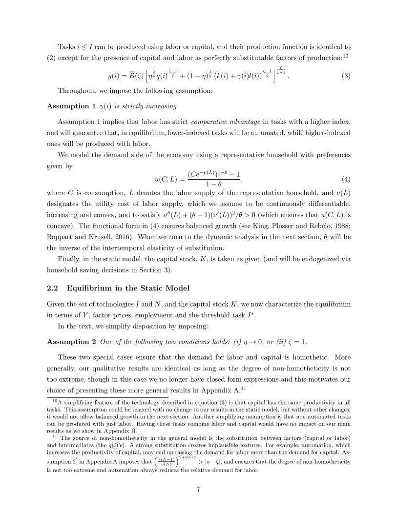
Tasks i ≤ I can be produced using labor or capital, and their production function is identical to

(2) except for the presence of capital and labor as perfectly substitutable factors of production:10

y(i) = B(ζ)[η

1ζ q(i)

ζ−1ζ + (1− η)

1ζ (k(i) + γ(i)l(i))

ζ−1ζ

] ζζ−1

. (3)

Throughout, we impose the following assumption:

Assumption 1 γ(i) is strictly increasing

Assumption 1 implies that labor has strict comparative advantage in tasks with a higher index,

and will guarantee that, in equilibrium, lower-indexed tasks will be automated, while higher-indexed

ones will be produced with labor.

We model the demand side of the economy using a representative household with preferences

given by

u(C,L) =(Ce−ν(L))1−θ − 1

1− θ, (4)

where C is consumption, L denotes the labor supply of the representative household, and ν(L)

designates the utility cost of labor supply, which we assume to be continuously differentiable,

increasing and convex, and to satisfy ν ′′(L) + (θ − 1)(ν ′(L))2/θ > 0 (which ensures that u(C,L) is

concave). The functional form in (4) ensures balanced growth (see King, Plosser and Rebelo, 1988;

Boppart and Krusell, 2016). When we turn to the dynamic analysis in the next section, θ will be

the inverse of the intertemporal elasticity of substitution.

Finally, in the static model, the capital stock, K, is taken as given (and will be endogenized via

household saving decisions in Section 3).

2.2 Equilibrium in the Static Model

Given the set of technologies I and N , and the capital stock K, we now characterize the equilibrium

in terms of Y , factor prices, employment and the threshold task I∗.

In the text, we simplify disposition by imposing:

Assumption 2 One of the following two conditions holds: (i) η → 0, or (ii) ζ = 1.

These two special cases ensure that the demand for labor and capital is homothetic. More

generally, our qualitative results are identical as long as the degree of non-homotheticity is not

too extreme, though in this case we no longer have closed-form expressions and this motivates our

choice of presenting these more general results in Appendix A.11

10A simplifying feature of the technology described in equation (3) is that capital has the same productivity in alltasks. This assumption could be relaxed with no change to our results in the static model, but without other changes,it would not allow balanced growth in the next section. Another simplifying assumption is that non-automated taskscan be produced with just labor. Having these tasks combine labor and capital would have no impact on our mainresults as we show in Appendix B.

11 The source of non-homotheticity in the general model is the substitution between factors (capital or labor)and intermediates (the q(i)’s). A strong substitution creates implausible features. For example, automation, whichincreases the productivity of capital, may end up raising the demand for labor more than the demand for capital. As-

sumption 2′

in Appendix A imposes that(

γ(N−1)γ(N)

)2+2σ+η

> |σ−ζ|, and ensures that the degree of non-homotheticity

is not too extreme and automation always reduces the relative demand for labor.

7

We proceed by characterizing the unit cost of producing each task as a function of factor prices

and the automation possibilities represented by I. Because tasks are produced competitively, their

price, p(i), will be equal to the minimum unit cost of production:

p(i) =

min

{R,

W

γ(i)

}1−η

if i ≤ I,(W

γ(i)

)1−η

if i > I,

(5)

where W denotes the wage rate and R denotes the rental rate of capital.

In equation (5), the unit cost of production for tasks i > I is given by the effective cost of

labor, W/γ(i) (which takes into account that the productivity of labor in task i is γ(i)). The unit

cost of production for tasks i ≤ I, on the other hand, depends on min{R, W

γ(i)

}reflecting the fact

that capital and labor are perfect substitutes in the production of automated tasks. In these tasks,

firms will choose whichever factor has a lower effective cost—R or W/γ(i).

Because labor has a strict comparative advantage in tasks with a higher index, the expression

for p(i) implies that there is a (unique) threshold I such that

W

R= γ(I). (6)

This threshold represents the task for which the costs of producing with capital and labor are equal.

For all tasks i < I, we have R < W/γ(i), and without any other constraints, these tasks will be

produced with capital. However, if I > I, firms cannot use capital all the way up to task I because

of the constraint imposed by the available automation technology. This implies that there exists a

unique equilibrium threshold task

I∗ = min{I, I}

such that all tasks i < I∗ will be produced with capital, while all tasks i > I∗ will be produced

with labor.12

Figure 2 depicts the resulting allocation of tasks to factors and also shows how, as already

noted, the creation of new tasks replaces existing tasks from the bottom of the distribution.

As noted in footnote 9, we have simplified the exposition by imposing that new tasks created at

N immediately replace tasks located at N − 1, and it is therefore profitable to produce new tasks

with labor (and hence we have not distinguished N , N∗ and N). In the static model, this will be

the case when the capital stock is not too large, which is imposed in the next assumption.

Assumption 3 Let K be such that R = Wγ(N) . We have K < K.

This assumption ensures that R > Wγ(N) and consequently that new tasks will increase aggregate

output and will be adopted immediately. Outside of this region, new tasks would not be utilized,

12Without loss of generality, we impose that firms use capital when they are indifferent between using capital orlabor, which explains our convention of writing that all tasks i ≤ I∗ (rather than i < I∗) are produced using capital.

8

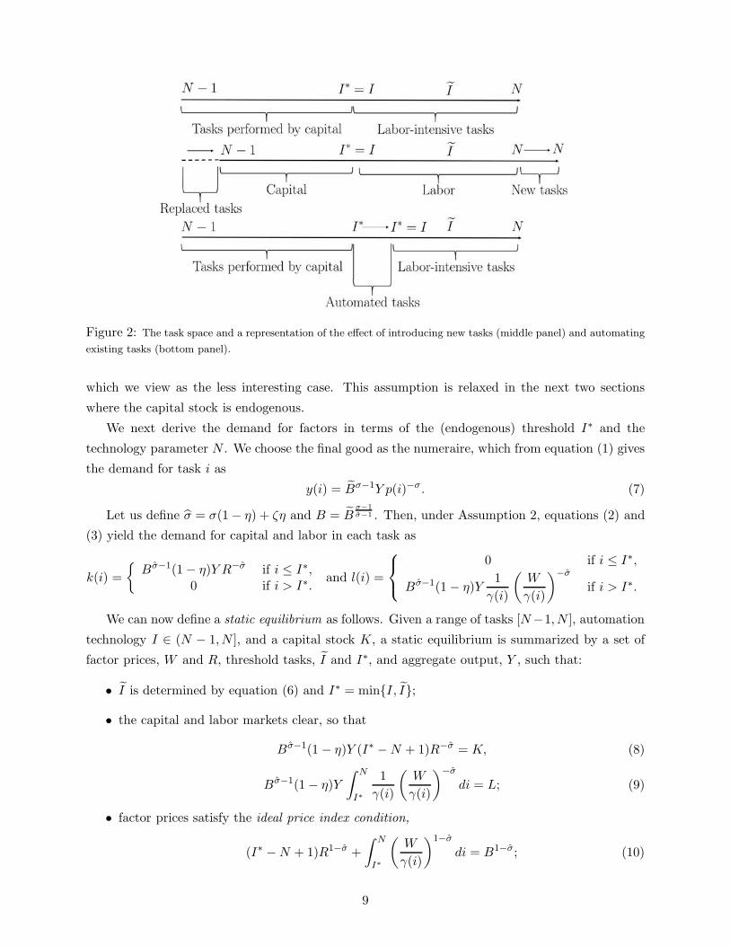
Figure 2: The task space and a representation of the effect of introducing new tasks (middle panel) and automating

existing tasks (bottom panel).

which we view as the less interesting case. This assumption is relaxed in the next two sections

where the capital stock is endogenous.

We next derive the demand for factors in terms of the (endogenous) threshold I∗ and the

technology parameter N . We choose the final good as the numeraire, which from equation (1) gives

the demand for task i as

y(i) = Bσ−1Y p(i)−σ. (7)

Let us define σ = σ(1− η) + ζη and B = Bσ−1σ−1 . Then, under Assumption 2, equations (2) and

(3) yield the demand for capital and labor in each task as

k(i) =

{Bσ−1(1− η)Y R−σ if i ≤ I∗,

0 if i > I∗.and l(i) =

0 if i ≤ I∗,

Bσ−1(1− η)Y1

γ(i)

(W

γ(i)

)−σ

if i > I∗.

We can now define a static equilibrium as follows. Given a range of tasks [N−1, N ], automation

technology I ∈ (N − 1, N ], and a capital stock K, a static equilibrium is summarized by a set of

factor prices, W and R, threshold tasks, I and I∗, and aggregate output, Y , such that:

• I is determined by equation (6) and I∗ = min{I, I};

• the capital and labor markets clear, so that

Bσ−1(1− η)Y (I∗ −N + 1)R−σ = K, (8)

Bσ−1(1− η)Y

∫ N

I∗

1

γ(i)

(W

γ(i)

)−σ

di = L; (9)

• factor prices satisfy the ideal price index condition,

(I∗ −N + 1)R1−σ +

∫ N

I∗

(W

γ(i)

)1−σ

di = B1−σ; (10)

9

• labor supply satisfies ν ′(L) = W/C. Since in equilibrium C = RK +WL, equilibrium labor

supply is implicitly given by the increasing labor supply function:13

L = Ls

(W

RK

). (11)

Proposition 1 (Equilibrium in the static model) Suppose that Assumptions 1, 2 and 3 hold.

Then a static equilibrium exists and is unique. In this static equilibrium, aggregate output is given

by

Y =B

1− η

(I∗ −N + 1)

1σK

σ−1σ +

(∫ N

I∗γ(i)σ−1di

) 1σ

Lσ−1σ

σσ−1

. (12)

Proof. See Appendix A.

Equation (12) shows that aggregate output is a CES aggregate of capital and labor, with the

elasticity between capital and labor being σ. The share parameters are endogenous and depend on

the state of the two types of technologies in the economy. An increase in I∗—which corresponds

to greater equilibrium automation—increases the share of capital and reduces the share of labor in

this aggregate production function, while the creation of new tasks does the opposite.

Figure 3 illustrates the unique equilibrium described in Proposition 1. The equilibrium is given

by the intersection of two curves in the (ω, I) space, where ω = WRK is the wage level normalized by

capital income; this ratio is a monotone transformation of the labor share and will play a central role

in the rest of our analysis.14 The upward-sloping curve represents the cost-minimizing allocation

of capital and labor to tasks represented by equation (6), with the constraint that the equilibrium

level of automation can never exceed I. The downward-sloping curve, ω(I∗, N,K), corresponds to

the relative demand for labor, which can be obtained directly by differentiating equation (12) as

lnω +1

σlnLs(ω) =

(1

σ− 1

)lnK +

1

σln

(∫ NI∗ γ(i)

σ−1di

I∗ −N + 1

). (13)

As we show in Appendix A, the relative demand curve always starts above the cost minimization

condition and ends up below it, so that the two curves necessarily intersect, defining a unique

equilibrium, as shown in Figure 3.

The figure also distinguishes between the two cases highlighted above. In the left panel, we have

I∗ = I < I and the allocation of factors is constrained by technology, while the right panel plots

the case where I∗ = I < I and firms choose the cost-minimizing allocation given factor prices.

A special case of Proposition 1 is also worth highlighting, because it leads to a Cobb-Douglas

production function with an exponent depending on the degree of automation, which is particularly

tractable in certain applications.

13This representation clarifies that the equilibrium implications of our setup are identical to one in which an upward-sloping quasi-labor supply determines the relationship between employment and wages (and does not necessarilyequate marginal cost of labor supply to the wage). This follows readily by taking (11) to represent this quasi-labor supply relationship. Appendix B provides a non-competitive micro-foundation for such a quasi-labor supplyrelationship.

14The increasing labor supply relationship, (11), ensures that the labor share sL = WLRK+WL

is increasing in ω.

10

Figure 3: Static equilibrium. The left panel depicts the case in which I∗ = I < I so that the allocation of factors

is constrained by technology. The right panel depicts the case in which I∗ = I < I so that the allocation of factors

is not constrained by technology and is cost-minimizing. The blue curves show the shifts following an increase in I

to I ′, which reduce ω in the left panel, but have no effect in the right panel.

Corollary 1 Suppose that σ = ζ = 1 and γ(i) = 1 for all i. Then aggregate output is

Y =B

1− ηK1−N+I∗LN−I∗ .

The next two propositions give a complete characterization of comparative statics.15

Proposition 2 (Comparative statics) Suppose that Assumptions 1, 2 and 3 hold. Let εL > 0

denote the elasticity of the labor supply schedule Ls(ω); let εγ = d ln γ(I)dI > 0 denote the semi-

elasticity of the comparative advantage schedule; and let

ΛI =γ(I∗)σ−1

∫ NI∗ γ(i)

σ−1di+

1

I∗ −N + 1and ΛN =

γ(N)σ−1

∫ NI∗ γ(i)

σ−1di+

1

I∗ −N + 1.

• If I∗ = I < I—so that the allocation of tasks to factors is constrained by technology—then:

– the impact of technological change on relative factor prices is given by

d ln(W/R)

dI=d lnω

dI=−

1

σ + εLΛI < 0,

d ln(W/R)

dN=d lnω

dN=

1

σ + εLΛN > 0;

– and the impact of capital on relative factor prices is given by

d ln(W/R)

d lnK=d lnω

d lnK+ 1 =

1 + εLσ + εL

> 0.

• If I∗ = I < I—so that the allocation of tasks to factors is cost-minimizing—then:

– the impact of technological change on relative factor prices is given by

d ln(W/R)

dI=d lnω

dI= 0,

d ln(W/R)

dN=d lnω

dN=

1

σfree + εLΛN > 0,

where

σfree = σ +1

εγΛI > σ;

15In this proposition, we do not explicitly treat the case in which I∗ = I = I in order to save on space and notation,since in this case left and right derivatives with respect to I are different.

11

– and the impact of capital on relative factor prices is given by

d ln(W/R)

d lnK=d lnω

d lnK+ 1 =

1 + εLσfree + εL

> 0.

• In all cases, the labor share and employment move in the same direction as ω. In particular,dLdN > 0 and, when I∗ = I, dL

dI < 0.

Proof. The proof follows by straightforward differentiation of the relevant terms and is provided

in Appendix B for completeness.

The main implication of Proposition 2 is that the two types of technological changes—automation

and the creation of new tasks—have polar implications. An increase in I—an improvement in au-

tomation technology—reduces W/R, the labor share and employment (unless I∗ = I < I and firms

are not constrained by technology in their automation choice), while an increase in N—the creation

of new tasks—raises W/R, the labor share and employment.16

Importantly, when I∗ = I < I, automation always reduces employment. Because automation

raises aggregate output per worker more than it raises the wage (automation may even reduce the

equilibrium wage as we will see next), the negative income effect on labor supply resulting from

the greater aggregate output dominates any substitution effect that might follow from the higher

wage. On the other hand, the creation of new tasks always increase employment—new tasks raise

the wage more than aggregate output, increasing labor supply. Although these exact results rely

on the balanced growth preferences in equation (4), similar forces operate in general and create a

tendency for automation to reduce employment and for new tasks to increase it.

These comparative static results are illustrated in Figure 3 as well: automation moves us along

the relative labor demand curve in the technology-constrained case shown in the left panel (and has

no impact in the right panel), while the creation of new tasks shifts out the relative labor demand

curve in both cases.

A final implication of Proposition 2 is that the “technology-constrained” elasticity of substitu-

tion between capital and labor, σ, which applies when I∗ = I < I, differs from the “technology-free”

elasticity, σfree , which applies when the decision of which tasks to automate is not constrained by

technology (i.e., when I∗ = I < I). This is because in the former case, as relative factor prices

change, the set of tasks performed by each factor remains fixed. In the latter case, as relative factor

prices change, firms reassign tasks to factors. This additional margin of adjustment implies that

σfree > σ.

Proposition 3 (Impact of technology on productivity, wages, and factor prices) Suppose

that Assumptions 1, 2 and 3 hold, and denote the changes in productivity—the change in aggregate

output holding capital and labor constant—by d lnY |K,L.

16Throughout, by “automation” or “automation technology” we refer to I , and use “equilibrium automation” torefer to I∗.

12

• If I∗ = I < I—so that the allocation of tasks to factors is constrained by technology—thenW

γ(I∗) > R > Wγ(N) , and

d ln Y |K,L =Bσ−1

1− σ

((W

γ(I∗)

)1−σ

−R1−σ

)dI +

Bσ−1

1− σ

(R1−σ −

(W

γ(N)

)1−σ)dN.

That is, both technologies increase productivity.

Moreover, let sL denote the labor share. The impact of technology on factor prices in this

case is given by:

d lnW =d ln Y |K,L + (1− sL)

(1

σ + εLΛNdN −

1

σ + εLΛIdI

),

d lnR =d ln Y |K,L − sL

(1

σ + εLΛNdN −

1

σ + εLΛIdI

).

That is, a higher N always increases the equilibrium wage but may reduce the rental rate,

while a higher I always increases the rental rate but may reduce the equilibrium wage. In

particular, there exists K > K such that an increase in I increases the equilibrium wage when

K < K and reduces it when K > K.

• If I∗ = I < I—so that the allocation of tasks to factors is not constrained by technology—thenW

γ(I∗) = R > Wγ(N) , and

d ln Y |K,L =Bσ−1

1− σ

(R1−σ −

(W

γ(N)

)1−σ)dN.

That is, new tasks increase productivity, but additional automation technologies do not.

Moreover, the impact of technology on factor prices in this case is given by:

d lnW =d lnY |K,L + (1− sL)1

σfree + εLΛNdN

d lnR =d lnY |K,L − sL1

σfree + εLΛNdN.

That is, an increase in N (more new tasks) always increases the equilibrium wage but may

reduce the rental rate, while an increase in I (greater technological automation) has no effect

on factor prices.

Proof. See Appendix B.

The most important result in Proposition 3 is that, when I∗ = I < I, automation—an increase

in I—always increases aggregate output, but has an ambiguous effect on the equilibrium wage. On

the one hand, there is a positive productivity effect captured by the term d lnY |K,L: by substituting

cheaper capital for expensive labor, automation raises productivity, and hence the demand for labor

in the tasks that are not yet automated.17 Countering this, there is a negative displacement effect

17This discussion also clarifies that our productivity effect is similar to the productivity effect in models of offshoringsuch as Grossman and Rossi-Hansberg (2008), Rodriguez-Clare (2010) and Acemoglu, Gancia and Zilibotti (2015).In these models, the productivity effect results from the substitution of cheap foreign labor for domestic labor incertain tasks.

13

captured by the term 1σ+εL

ΛI . This negative effect occurs because automation contracts the set

of tasks performed by labor. Because tasks are subject to diminishing returns in the aggregate

production function, (1), bunching workers into fewer tasks puts downward pressure on the wage.

As the equation for d lnY |K,L reveals, the productivity gains depend on the cost savings from

automation, which are given by the difference between the effective wage at I∗, Wγ(I∗) , and the

rental rate, R. When the productivity gains are small—which is guaranteed when K > K—the

gap between Wγ(I∗) and R is small, and so is the productivity effect; in this case, the overall impact

is necessarily negative.

Finally, Proposition 3 shows that an increase in N always increases productivity and the equi-

librium wage (recall that Assumption 3 imposes that R > Wγ(N)), and when the productivity gains

from the creation of new tasks are small, it can reduce the rental rate.

The fact that automation may increase productivity while simultaneously reducing wages is

a key feature of the task-based framework developed here. With factor-augmenting technologies,

capital-augmenting technological improvements always increase the equilibrium wage, but this is no

longer the case when technological change alters the range of tasks performed by both factors (see

also Acemoglu and Autor, 2011).18 Furthermore, with factor-augmenting technologies, whether

different types of technological improvements are biased towards one factor or the other, and hence

their impact on factor shares, depends on the elasticity of substitution. But this too is different in

our task-based framework; here automation is always capital-biased (that is, it reduces both W/R

and the labor share), while the creation of new tasks is always labor-biased (that is, it increases

both W/R and the labor share).

3 Dynamics and Balanced Growth

In this section, we extend our model to a dynamic economy in which the evolution of the capital

stock is determined by the saving decisions of the representative household. We then investigate

the conditions under which the economy admits a balanced growth path (BGP), where aggregate

output, the capital stock and wages grow at a constant rate. We conclude by discussing the long-run

effects of automation on wages, the labor share and employment.

3.1 Balanced Growth

We assume that the representative household’s dynamic preferences are given by

∫ ∞

0e−ρtu(C(t), L(t))dt, (14)

where u(C(t), L(t)) is as defined in equation (4) and ρ > 0 is the discount rate.

18For instance, with a constant returns to scale production function and two factors, capital and labor areq−complements. Thus, capital-augmenting technologies always increases the marginal product of labor . To seethis, let F (AKK,ALL) be such a production function. Then W = FL, and

dWdAK

= KFLK = −LFLL > 0 (because of

constant returns to scale).

14

To ensure balanced growth, we impose more structure to the comparative advantage schedule.

Because balanced growth is driven by technology, and in this model sustained technological change

comes from the creation of new tasks, constant growth requires the productivity gains from new

tasks to be exponential.19 Thus, in what follows we strengthen Assumption 1 to:

Assumption 1′ γ(i) satisfies:

γ(i) = eAi with A > 0. (15)

The path of technology, represented by {I(t), N(t)}, is exogenous, and we define

n(t) = N(t)− I(t)

as a summary measure of technology, and similarly let n∗(t) = N(t)− I∗(t) be a summary measure

of the state of technology used in equilibrium (since I∗(t) ≤ I(t), we have n∗(t) ≥ n(t)). New

automation technologies reduce n(t), while the introduction of new tasks increases it.

From equation (12), aggregate output net of intermediates, or simply “net output,” can be

written as a function of technology represented by n∗(t) and γ(I∗(t)) = eAI∗(t), the capital stock,

K(t), and the level of employment, L(t), as

F(K(t), eAI(t)L(t);n∗(t)

)= B

(1− n∗(t))

1σK(t)

σ−1σ +

(∫ n∗(t)

0γ(i)σ−1di

) 1σ

eAI∗(t)L(t))σ−1σ

σσ−1

.

(16)

The resource constraint of the economy then takes the form

K(t) = F(K(t), eAI(t)L(t);n∗(t)

)− C(t)− δK(t),

where δ is the depreciation rate of capital.

We characterize the equilibrium in terms of the employment level L(t), and the normalized

variables k(t) = K(t)e−AI∗(t), and c(t) = C(t)e1−θθ

ν(L(t))−AI∗(t). As in our static model, R(t) denotes

the rental rate, and w(t) = W (t)e−AI∗(t) is the normalized wage. These normalized variables

determine factor prices as:

R(t) =FK [k(t), L(t);n∗(t)]

=B(1− n∗(t))1σ

(1− n∗(t))

1σ +

(∫ n∗(t)

0γ(i)σ−1di

) 1σ (L(t)

k(t)

) σ−1σ

1σ−1

19Notice also that in this dynamic economy, as in our static model, the productivity of capital is the same in allautomated tasks. This does not, however, imply that any of the previously automated tasks can be used regardless ofN . As N increases, as emphasized by equation (1) and in footnote 9, the set of feasible tasks shifts to the right, andonly tasks above N − 1 remain compatible with and can be combined with those currently in use. Just to cite a fewmotivating examples for this assumption: power looms of the 18th and 19th century are not compatible with moderntextile technology; assembly lines based on the dedicated machinery are not compatible with numerically controlledmachines and robots; first-generation calculators are not compatible with computers; and bookkeeping methods fromthe 19th and 20th centuries are not compatible with the modern, computerized office.

15

and

w(t) =FL[k(t), L(t);n∗(t)]

=B

(∫ n∗(t)

0γ(i)σ−1di

) 1σ

(1− n(t))

1σ

(k(t)

L(t)

) σ−1σ

+

(∫ n(t)

0γ(i)σ−1di

) 1σ

1σ−1

.

The equilibrium interest rate is R(t)− δ.

Given time paths for g(t) (the growth rate of eAI(t)) and n(t), a dynamic equilibrium can

now be defined as a path for the threshold task n∗(t), (normalize) capital and consumption, and

employment, {k(t), c(t), L(t)}, that satisfies

• n∗(t) ≥ n(t), with n∗(t) = n(t) only if w(t) > R(t), and n∗(t) > n(t) only if w(t) = R(t);

• the endogenous labor supply condition,

ν ′(L(t))eθ−1θ

ν(L(t)) =FL[k(t), L(t);n

∗(t)]

c(t); (17)

• the Euler equation,

c(t)

c(t)=

1

θ(FK [k(t), L(t);n∗(t)]− δ − ρ)− g(t); (18)

• the representative household’s transversality condition,

limt→∞

k(t)e−∫ t

0(FK [k(s),L(s);n∗(s)]−δ−g(s))ds = 0; (19)

• and the resource constraint,

k(t) = F (k(t), L(t);n∗(t))− c(t)e−1−θθ

ν(L(t)) − (δ + g(t))k(t). (20)

We also define a balanced growth path (BGP) as a dynamic equilibrium in which the economy

grows at a constant rate, factor shares are constant, and the rental rate of capital R(t) is constant.

To characterize the growth dynamics implied by these equations, let us first consider a path

for technology such that g(t) → g and n(t) → n, consumption grows at the rate g and the Euler

equation holds R(t) = ρ + δ + θg. Suppose first that n∗(t) = n(t) = 0, in which case F becomes

linear and R(t) = B. Because the growth rate of consumption must converge to g as well, the Euler

equation (18) is satisfied in this case only if ρ is equal to

ρ = B − δ − θg. (21)

Lemma A2 in Appendix A shows that this critical value of the discount rate divides the parameter

space into two regions as shown in Figure 4. To the left of ρ, there exists a decreasing curve n(ρ)

defined over [ρmin, ρ] with n(ρ) = 0, and to the right of ρ, there exists an increasing curve n(ρ)

defined over [ρ, ρmax] with n(ρ) = 0, such that:20

20The functions wN (n) and wI(n) depicted in this figure are introduced below.

16

• for n > n(ρ), we have w(t)γ(N(t)) < R(t) and new tasks raise aggregate output and are immediately

produced with labor;

• for n > n(ρ), we have w(t) > R(t) and automated tasks raise aggregate output and are

immediately produced with capital; and

• for n < n(ρ), we have w(t) < R(t) and small changes in automation do not affect n∗ and

other equilibrium objects.

Figure 4: Behavior of factor prices in different parts of the parameter space.

The next proposition provides the conditions under which a BGP exists, and characterizes the

BGP that results in each case. In what follows, we no longer impose Assumption 3, since depending

on the value of ρ, the capital stock can become large and induce full automation.

Proposition 4 (Dynamic equilibrium with exogenous technological change) Suppose that

Assumptions 1′ and 2 hold. The economy admits a BGP if only if we are in one of the following

cases:

1. (Full automation) if ρ < ρ and N(t) = I(t) with B > δ + ρ > 1−θθ (B − δ − ρ) + δ, then

there exists a unique and globally stable BGP. Moreover, in this BGP n∗(t) = 0, all tasks are

produced with capital, and the labor share is zero;

2. (Interior BGP with immediate automation) if N(t) = I(t) = ∆ with ρ+(θ−1)A∆ > 0

and n(t) = n > max{n(ρ), n(ρ)}, then there exists a unique and globally stable BGP. In this

BGP n∗(t) = n and I∗(t) = I(t).

17

3. (Interior BGP with eventual automation) if ρ > ρ, N(t) = ∆ and I(t) ≥ ∆ with

ρ + (θ − 1)A∆ > 0, and n(t) < n(ρ), then there exists a unique and globally stable BGP. In

this BGP n∗(t) = n(ρ) and I∗(t) = I(t) > I(t).

4. (No automation) if ρ > ρmin and N(t) = ∆ with ρ + (θ − 1)A∆ > 0, then there exists a

unique and globally stable BGP. In this BGP all tasks are produced with labor, and the capital

share is zero.

Proof. See Appendix A.

The first type of BGP in Proposition 4 involves the automation of all tasks, in which case

aggregate output becomes linear in capital. This case was ruled out by Assumption 3 in our static

analysis, but as the proposition shows, when the discount rate, ρ, is sufficiently small, it can emerge

in the dynamic model. A BGP with no automation (case 4), where growth is driven entirely by

the creation of new tasks, is also possible if the discount rate is sufficiently large.

More important for our focus are the two interior BGPs where automation and the introduction

of new tasks go hand-in-hand, and as a result, n∗(t) is constant at some value between 0 and 1;

this implies that both capital and labor perform a fixed measure of tasks. In the more interesting

case where automated tasks are immediately produced with capital (case 2), the proposition also

highlights that this process needs to be “balanced” itself: the two types of technologies need to

advance at the same rate so that n(t) = n.

Balanced growth with constant labor share emerges in this model because the net effect of

automation and the creation of new technologies proceeding at the same rate is to augment labor

while keeping constant the share of tasks performed by labor—as shown by equation (16). In this

case, the gap between the two types of technologies, n(t), regulates the share parameters in the

resulting CES production function, while the levels of N(t) and I(t) determine the productivity

of labor in the set of tasks that it performs. When n(t) = n, technology becomes purely labor

augmenting on net because labor performs a fixed share of tasks, and labor becomes more productive

over time in producing the newly-created tasks.21

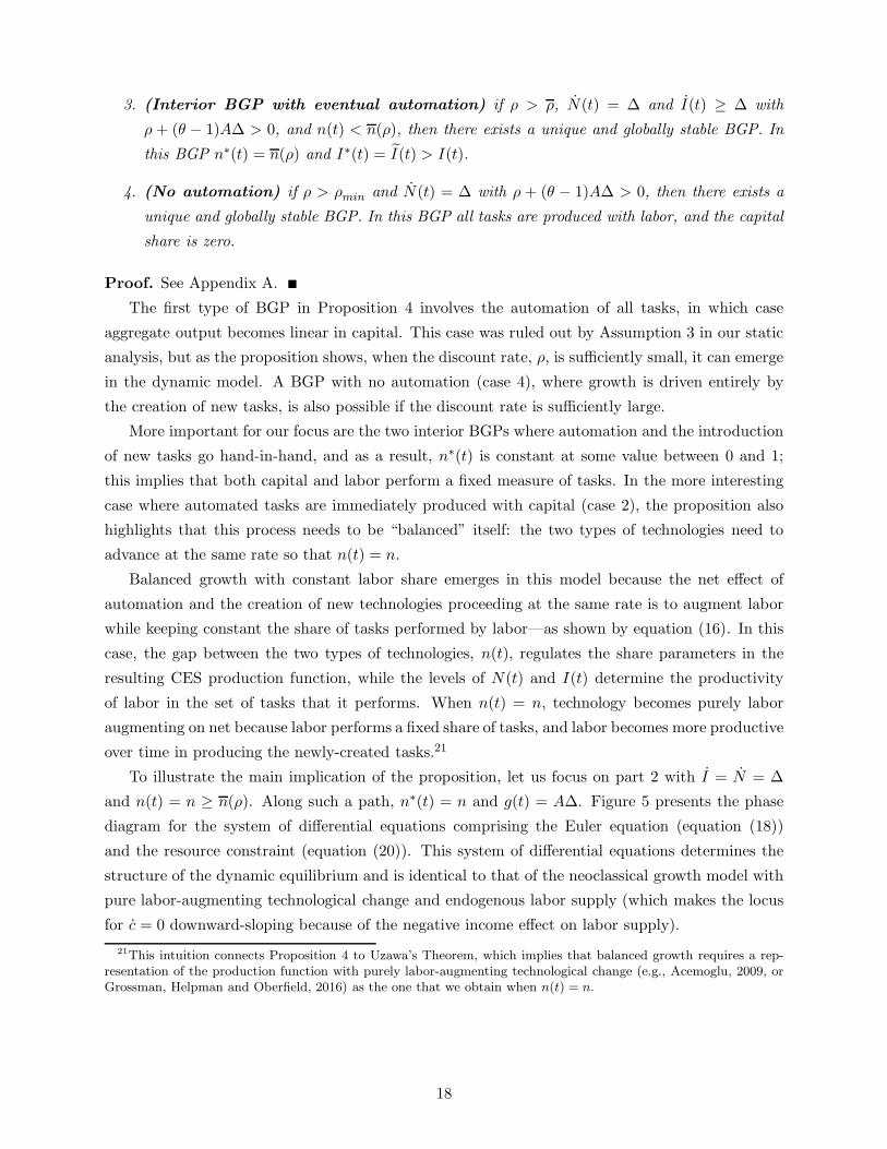
To illustrate the main implication of the proposition, let us focus on part 2 with I = N = ∆

and n(t) = n ≥ n(ρ). Along such a path, n∗(t) = n and g(t) = A∆. Figure 5 presents the phase

diagram for the system of differential equations comprising the Euler equation (equation (18))

and the resource constraint (equation (20)). This system of differential equations determines the

structure of the dynamic equilibrium and is identical to that of the neoclassical growth model with

pure labor-augmenting technological change and endogenous labor supply (which makes the locus

for c = 0 downward-sloping because of the negative income effect on labor supply).

21This intuition connects Proposition 4 to Uzawa’s Theorem, which implies that balanced growth requires a rep-resentation of the production function with purely labor-augmenting technological change (e.g., Acemoglu, 2009, orGrossman, Helpman and Oberfield, 2016) as the one that we obtain when n(t) = n.

18

Figure 5: Dynamic equilibrium when technology is exogenous and satisfies n(t) = n and g(t) = A∆.

3.2 Long-Run Comparative Statics

We next study the log-run implications of an unanticipated and permanent decline in n(t), which

corresponds to automation running ahead of the creation of new tasks. Because in the short run

capital is fixed, the short-run implications of this change in technology are the same as in our

static analysis in the previous section. But the fact that capital adjusts implies different long-run

dynamics.

Consider an interior BGP in which N(t) − I(t) = n ∈ (0, 1). Along this path, the equilibrium

wage grows at the rate A∆. Define wI(n) = limt→∞W (t)/γ(I∗(t)) as the effective wage paid in the

least complex task produced with labor and wN (n) = limt→∞W (t)/γ(N(t)) as the effective wage

paid in the most complex task produced with labor. Both of these functions are defined well-defined

and thus depend only on n. Figure 4 shows how these effective wages compare to the BGP value

of the rental rate of capital, ρ+ δ + θg.

The next proposition characterizes the long-run impact of automation on factor prices, employ-

ment and the labor share in the interior BGPs.

Proposition 5 (Long-run comparative statics) Suppose that Assumptions 1′ and 2 hold. Con-

sider a path for technology in which n(t) = n ∈ (0, 1) and g(t) = g (so that we are in case 2 or 3

in Proposition 4). Then, in the unique BGP we have R(t) = ρ+ δ + θg, and

• for n < n(ρ), wI(n) = wI(n(ρ)) and wN (n) = wN (n(ρ)). Consequently, small changes in n

do not affect the paths of effective wages, employment and the labor share.

• For n > n(ρ), wI(n) is increasing and wN (n) is decreasing in n. Moreover, the asymptotic

values for employment and the labor share are increasing in n. Finally, if the increase in n

is caused by an increase in I, the capital stock also increases.

Proof. The proof is straightforward and is presented in Appendix B for completeness.

19

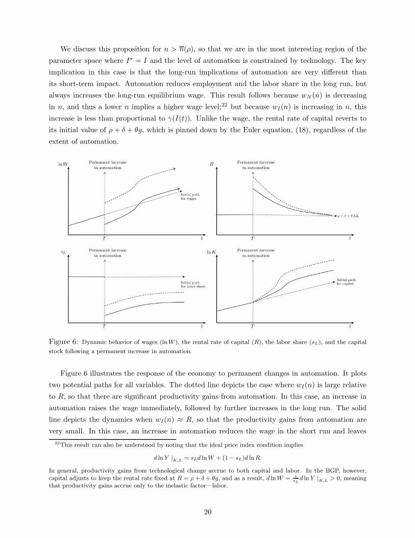
We discuss this proposition for n > n(ρ), so that we are in the most interesting region of the

parameter space where I∗ = I and the level of automation is constrained by technology. The key

implication in this case is that the long-run implications of automation are very different than

its short-term impact. Automation reduces employment and the labor share in the long run, but

always increases the long-run equilibrium wage. This result follows because wN (n) is decreasing

in n, and thus a lower n implies a higher wage level;22 but because wI(n) is increasing in n, this

increase is less than proportional to γ(I(t)). Unlike the wage, the rental rate of capital reverts to

its initial value of ρ + δ + θg, which is pinned down by the Euler equation, (18), regardless of the

extent of automation.

Figure 6: Dynamic behavior of wages (lnW ), the rental rate of capital (R), the labor share (sL), and the capital

stock following a permanent increase in automation.

Figure 6 illustrates the response of the economy to permanent changes in automation. It plots

two potential paths for all variables. The dotted line depicts the case where wI(n) is large relative

to R, so that there are significant productivity gains from automation. In this case, an increase in

automation raises the wage immediately, followed by further increases in the long run. The solid

line depicts the dynamics when wI(n) ≈ R, so that the productivity gains from automation are

very small. In this case, an increase in automation reduces the wage in the short run and leaves

22This result can also be understood by noting that the ideal price index condition implies

d lnY |K,L = sLd lnW + (1− sL)d lnR.

In general, productivity gains from technological change accrue to both capital and labor. In the BGP, however,capital adjusts to keep the rental rate fixed at R = ρ+ δ + θg, and as a result, d lnW = 1

sLd ln Y |K,L > 0, meaning

that productivity gains accrue only to the inelastic factor—labor.

20

it approximately unchanged in the long run. In contrast to the concerns that highly productive

automation technologies will reduce the wage and employment, our model thus shows that it is

precisely when automation fails to raise productivity significantly that it has a more detrimental

impact on wages and employment. In both cases, the duration of the period with stagnant or

depressed wages depends on θ, which determines the speed of capital adjustment following an

increase in the rental rate.

The remaining panels of the figure show that automation reduces employment and the labor

share, as stated in Proposition 5. If σ < 1, the resulting capital accumulation mitigates the short-

run decline in the labor share but does not fully offset it (this is the case depicted in the figure). If

σ > 1, capital accumulation further depresses the labor share—even though it raises the wage.

The long-run impact of a permanent increase in N(t) can also be obtained from the proposition.

In this case, new tasks increase the wage (because wI(n) is increasing in n), aggregate output,

employment, and the labor share, both in the short and the long run. Because the short-run impact

of new tasks on the rental rate of capital is ambiguous, so is the response of capital accumulation.

In light of these results, the recent decline in the labor share and the employment to population

ratio in the United States can be interpreted as a consequence of automation outpacing the creation

of new labor-intensive tasks. Faster automation relative to the creation of new tasks might be driven

by an acceleration in the rate at which I(t) advances, in which case we would have stagnant or

lower wages in the short run while capital adjusts to a new higher level. Alternatively, it might be

driven by a deceleration in the rate at which N(t) advances, in which case we would also have low

growth of aggregate output and wages. We return to the productivity implications of automation

once we introduce our full model with endogenous technological change in the next section.

4 Full Model: Tasks and Endogenous Technologies

The previous section established, under some conditions, the existence of an interior BGP with

N = I = ∆. This result raises a more fundamental question: why should these two types of

technologies advance at the same rate? To answer this question we now develop our full model,

which endogenizes the pace at which automation and the creation of new tasks proceeds.

4.1 Endogenous and Directed Technological Change

To endogenize technological change, we deviate from our earlier assumption of a perfectly compet-

itive market for intermediates, and assume that (intellectual) property rights to each intermediate,

q(i), are held by a technology monopolist which can produce it at the marginal cost µψ in terms of

the final good, where µ ∈ (0, 1) and ψ > 0. We also assume that this technology can be copied by

a fringe of competitive firms, which can replicate any available intermediate at a higher marginal

cost of ψ, and that µ is such that the unconstrained monopoly price of an intermediate is greater

than ψ. This ensures that the unique equilibrium price for all types of intermediates is a limit price

of ψ, and yields a per unit profit of (1−µ)ψ > 0 for technology monopolists. These profits generate

21

incentives for creating new tasks and automation technologies.

In this section, we adopt a structure of intellectual property rights that abstracts from the

creative destruction of profits. We assume that developing a new intermediate that automates or

replaces an existing task is viewed as an infringement of the patent of the technology previously

used to produce that task. Consequently, a firm must compensate the technology monopolist who

owns the property rights over the production of the intermediate that it is replacing. We also

assume that this compensation takes place with the new inventors making a take-it-or-leave-it offer

to the holder of the existing patent.

Developing new intermediates that embody technology requires scientists.23 There is a fixed

supply of S scientists, which will be allocated to automation (SI(t) ≥ 0) or the creation of new

tasks (SN (t) ≥ 0),

SI(t) + SN (t) ≤ S.

When a scientist is employed in automation, she automates κI tasks per unit of time and receives

a wage W SI (t). When she is employed in the creation of new tasks, she creates κN new tasks per

unit of time and receives a wage W SN (t). We assume that automation and the creation of new tasks

proceed in the order of the task index i. Thus, the allocation of scientists determines the evolution

of both types of technology—summarized by the level of I(t) and N(t)—as

I(t) = κISI(t), and N(t) = κNSN (t). (22)

Because we want to analyze the properties of the equilibrium locally, we make a final assumption

to ensure that the allocation of scientists varies smoothly when there is a small difference between

W SI (t) and W

SN (t) (rather than having discontinuous jumps). In particular, we assume that scien-

tists differ in the cost of effort: when working in automation, scientist j incurs a cost of χjIY (t), and

when working in the creation of new tasks, she incurs a cost of χjNY (t).24 Consequently, scientist j

will work in automation ifWS

I (t)−WSN (t)

Y (t) > χjN −χj

I . We also assume that the distribution of χiN −χiI

among scientists is given by a smooth and increasing distribution function G over a support [−υ, υ],

where we take υ to be small enough that χjN and χj

S are always less than max{

κNVN (t)Y (t) , κIVI(t)

Y (t)

}

and thus all scientists always work. For notational convenience, we also adopt the normalization

G(0) = κN

κI+κN.

4.2 Equilibrium with Endogenous Technological Change

We first compute the present discounted value accruing to monopolists from automation and the

creation of new tasks. Let VI(t) denote the value of automating task i = I(t) (i.e., the highest-

indexed task that has not yet been automated, or more formally i = I(t) + ε for ε arbitrarily small

and positive). Likewise, VN (t) is the value of a new technology creating a new task at i = N(t).

23Focusing on an innovation possibilities frontier using just scientists, rather than variable factors such as in thelab-equipment specifications (see Acemoglu 2009), is convenient because it enables us to focus on the direction oftechnological change—and not on the overall amount of technological change.

24The cost of effort is multiplied by Y (t) to capture the income effect on the costs of effort in a tractable manner.

22

To simplify the exposition, let us assume that in this equilibrium n(t) > max{n(ρ), n(ρ)}(ρ), so

that I∗(t) = I(t) and newly-automated tasks start being produced with capital immediately. The

flow profits that accrue to the technology monopolist that automated task i are:25

πI(t, i) = bY (t)R(t)ζ−σ, (23)

where b = (1− µ)Bσ−1ηψ1−ζ . Likewise, the flow profits that accrue to the technology monopolist

who created the labor-intensive task i are:

πN (t, i) = bY (t)

(W (t)

γ(i)

)ζ−σ

. (24)

The take-it-or-leave-it nature of offers implies that a firm that automates task I needs to com-

pensate the existing technology monopolist by paying her the present discounted value of the profits

that her inferior labor-intensive technology would generate if not replaced. This take-it-or-leave-it

offer is given by:26

b

∫ ∞

te−∫ τ

0(R(s)−δ)dsY (τ )

(W (τ)

γ(I)

)ζ−σ

dτ.

Likewise, a firm that creates task N needs to compensate the existing technology monopolist

by paying her the present discounted value of the profits from the capital-intensive alternative

technology. This take-it-or-leave-it offer is given by:

b

∫ ∞

te−∫ τ0 (R(s)−δ)dsY (τ)R(τ )ζ−σdτ .

In both cases, the patent-holders will immediately accept theses offers and reject less generous ones.

We can then compute the values of innovating and becoming a technology monopolist as:

VI(t) = bY (t)

∫ ∞

te−∫ τt(R(s)−δ−gy(s))ds

(R(τ )ζ−σ −

(w(τ )e

∫ τtg(s)ds

)ζ−σ)dτ , (25)

and

VN (t) = bY (t)

∫ ∞

te−∫ τ

t(R(s)−δ−gy(s))ds

((w(τ )

γ(n(t))e∫ τ

tg(s)ds

)ζ−σ

−R(τ)ζ−σ

)dτ, (26)

for automation and creation of new tasks, respectively, where gy(t) is the growth rate of aggregate

output at time t and as noted above, g(t) is the growth rate of γ(N(t)).

The expressions for the value functions, VI(t) and VN (t), share a common form: they subtract

the lower cost of producing a task with the factor for which the new technology is designed from

the higher cost of producing the same task with the older technology.27 Because new entrants

25This follows because the demand for intermediates is q(i) = Bσ−1ηψ−ζY (t)R(t)ζ−σ, each intermediate is sold ata price ψ, and the technology monopolist makes a per unit profit of 1− µ.

26This expression is written by assuming that the patent-holder will also turn down subsequent less generous offersin the future. Writing it using dynamic programming and the one-step ahead deviation principle leads to the sameconclusion.

27There is an important difference between the value functions in (25) and (26) and those in models of directedtechnological change building on factor-augmenting technologies (such as in Acemoglu, 1998, or 2002). In the lattercase, the direction of technological change is determined by the interplay of a market size effect favoring the more

23

compensate the incumbent technology monopolists that they replace, our patent structure removes

the creative destruction of profits, which is present in other models of quality improvements under

the alternative assumption that new firms do not have to respect the intellectual property rights of

the technology on which they are building (e.g., Aghion and Howitt, 1992; Grossman and Helpman,

1991). In Section 5, we explore how our main results change when the intellectual property rights

regime allows for the creative destruction of profits.

To ensure that the value functions are well-behaved and non-negative, for the rest of the paper

we impose the following assumption:

Assumption 4 σ > ζ.

This ensures that innovations are directed towards technologies that allow firms to produce

tasks by using the cheaper (or more productive) factors, and consequently, that the present dis-

counted values from innovation are positive. This assumption is intuitive and reasonable: since

intermediates embody the technology that directly works with labor or capital, they should be

highly complementary with the relevant factor of production in the production of tasks.28

An equilibrium with endogenous technology is given by paths {K(t), N(t), I(t)} for capital and

technology (starting from initial values K(0), N(0), I(0)), paths {R(t),W (t),W SI (t),W

SN (t)} for

factor prices, paths {VN (t), VI(t)} for the value functions of technology monopolists, and paths

{SN (t), SI(t)} for the allocation of scientists such that all markets clear, all firms and prospec-

tive technology monopolists maximize profits, the representative household maximizes its utility.

Using the same normalizations as in the previous section, we can represent the equilibrium with

endogenous technology by a path of the tuple {c(t), k(t), n(t), L(t), SI (t), VI(t), VN (t)} such that:

• consumption satisfies the Euler equation (18) and the labor supply satisfies equation (17);

• the transversality condition holds

limt→∞

(k(t) + Π(t))e−∫ t0 (ρ−(1−θ)g(s))ds = 0, (27)

abundant factor and a price effect favoring the cheaper factor. The task-based framework here, combined with theassumption on the structure of patents, makes the benefits of new technologies only a function of the factor prices—in particular, the difference between the wage rate and the rental rate. This is because factor prices determine theprofitability of producing with capital relative to labor. Without technological constraints, this would determine theset of tasks that the two factors perform. In the presence of technological constraints restricting which tasks can beproduced with which factor, factor prices then determine the incentives for automation (to expand the set of tasksproduced by capital) and the creation of new tasks (to expand the set of tasks produced by labor).

We should also note that despite this difference, the general results on absolute weak bias of technology in Acemoglu(2007) continue to hold here—in the sense that an increase in the abundance of a factor always makes technologymore biased towards that factor.

28The profitability of introducing an intermediate that embodies a new technology depends on its demand. As afactor (labor or capital) becomes cheaper, there are two effects. First, the decline in costs allows firms to scale uptheir production, which increases the demand for the intermediate good. The extent of this positive scale effect isregulated by the elasticity of substitution σ. Second, because the cheaper factor is substituted for the intermediateit is combined with, the demand for that intermediate good falls. This countervailing substitution effect is regulatedby the elasticity of substitution ζ. The condition σ > ζ guarantees that the former, positive effect dominates, sothat prospective technology monopolists have an incentive to introduce technologies that allow firms to produce tasksmore cheaply. When the opposite holds and ζ > σ, we have the paradoxical situation where technologies that workwith more expensive factors are more profitable, and consequently, in this case the present discounted values frominnovation is negative.

24

where in addition to the capital stock in equation (19), we now have the present value of

corporate profits Π(t) = I(t)VI(t)/Y (t) + N(t)VN (t)/Y (t) also added to the representative

household’s budget;

• capital satisfies the resource constraint

k(t) =

[1 +

η

1− η(1− µ)

]F (k(t), L(t);n∗(t))− c(t)e−

1−θθ

ν(L(t)) − (δ + g(t))k(t),

where recall that F (k(t), L(t);n∗(t)) is net output (aggregate output net of intermediates)

and η1−η (1− µ)F (k(t), L(t);n∗(t)) is profits of technology monopolists from intermediates;

• competition among prospective technology monopolists to hire scientists implies thatW SI (t) =

κIVI(t) and WSN (t) = κNVN (t). Thus,

SI(t) = SG

(κIVI(t)

Y (t)−κNVN (t)

Y (t)

), SN (t) = S

[1−G

(κIVI(t)

Y (t)−κNVN (t)

Y (t)

)]S,

and n(t) according to:

n(t) = κNS − (κN + κI)G

(κIVI(t)

Y (t)−κNVN (t)

Y (t)

); (28)

• and the value functions that determine the allocation of scientists, VI(t) and VN (t), are given

by (25) and (26).

As before, a BGP is given by an equilibrium in which the normalized variables c(t), k(t) and

L(t), and the rental rate R(t) are constant, except that now n(t) is determined endogenously. The

definition of the equilibrium shows that the profits from automation and the creation of new tasks

determine the evolution of n(t): whenever one of the two types of innovation is more profitable,

more scientists will be allocated to that activity.

Consider an allocation where n(t) = n ∈ (0, 1). Let us define the normalized value functions

vI(n) = limt→∞ VI(t)/Y (t) and vN (n) = limt→∞ VN (t)/Y (t), which only depend on n. Equation

(28) implies that n(t) > 0 if and only if κNVN (t) > κIVI(t), and n(t) < 0 if and only if κNVN (t) <

κIVI(t). Thus if κIvI(n) 6= κNvN (n), the economy converges to a corner with n(t) equal to 0 or 1,

and for an interior BGP with n ∈ (0, 1) we need

κIvI(n) = κNvN (n). (29)

The next proposition gives the main result of the paper, and characterizes different types of

BGPs with endogenous technology.

Proposition 6 (Equilibrium with endogenous technological change) Suppose that Assump-

tions 1′, 2, and 4 hold. Then, there exists S such that, when S < S, we have:29

29The condition S < S ensures that the growth rate of the economy is not too high. If the growth rate is abovethe threshold implied by S, the creation of new tasks is discouraged (even if current wages are low) because firmsanticipate that the wage will grow rapidly, reducing the future profitability of creating new labor-intensive tasks.This condition also allows us to use Taylor approximations of the value functions in our analysis of local stability.

25

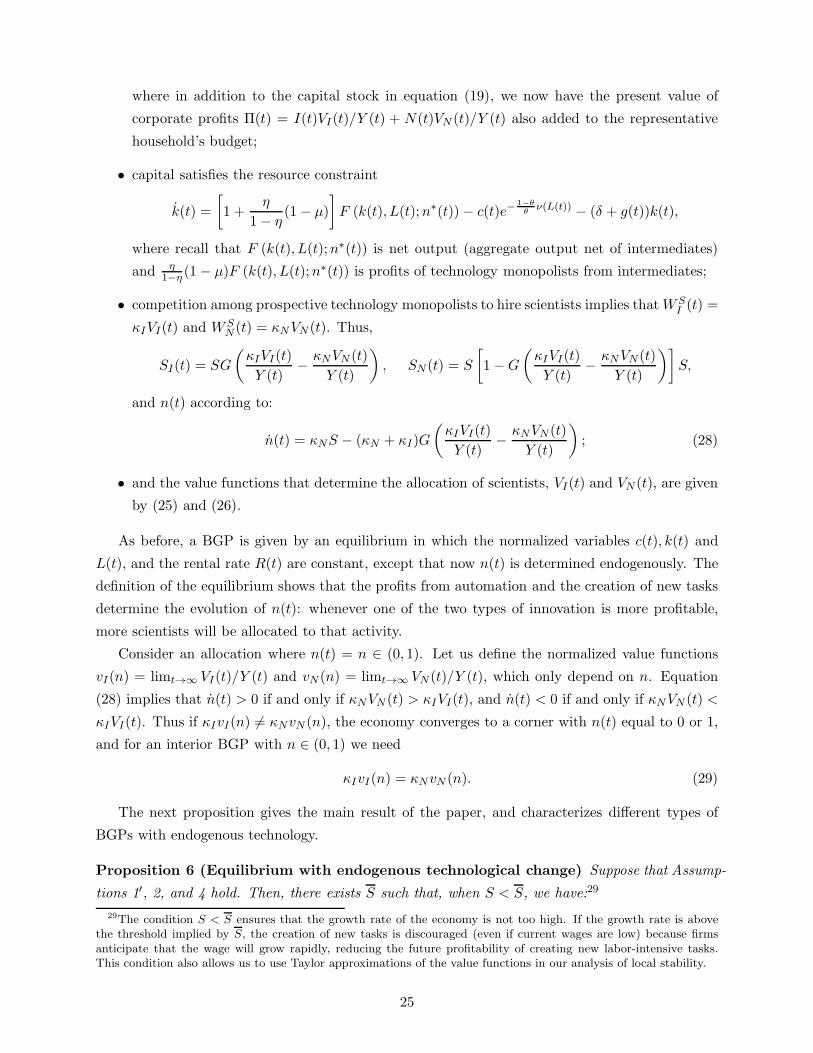
1 (Full automation) For ρ < ρ, there is a BGP in which n(t) = 0 and all tasks are produced

with capital.

For ρ > ρ, all BGPs feature n(t) = n > n(ρ). Moreover, there exist κ ≥ κ > 0 such that:

2 (Unique interior BGP) if κI

κN> κ there exists a unique BGP. In this BGP we have

n(t) = n ∈ (n(ρ), 1) and κNvN (n) = κIvI(n). If, in addition, θ = 0, then the equilibrium is

unique everywhere and the BGP is globally (saddle-path) stable. If θ > 0, then the equilibrium

is unique in the neighborhood of the BGP and is asymptotically (saddle-path) stable;

3 (Multiple BGPs) if κ > κI

κN> κ, there are multiple BGPs;

4 (No automation) If κ > κI

κN, there exists a unique BGP. In this BGP n(t) = 1 and all tasks

are produced with labor.

Proof. See Appendix A.

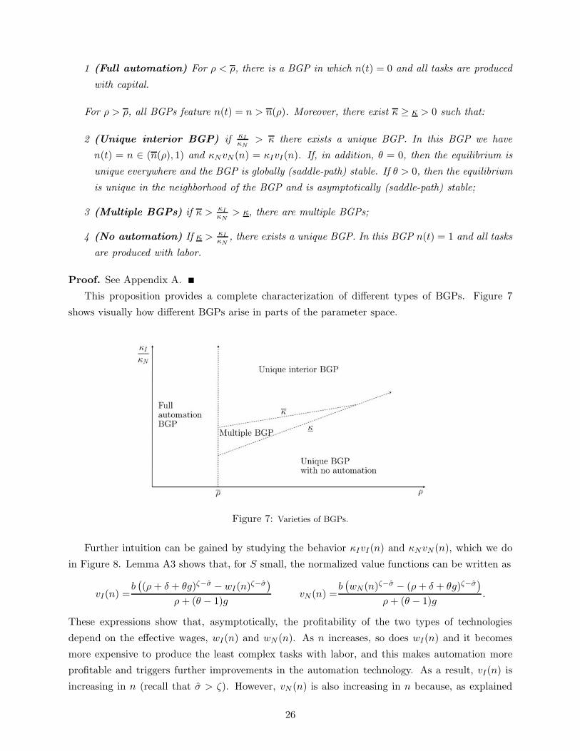
This proposition provides a complete characterization of different types of BGPs. Figure 7

shows visually how different BGPs arise in parts of the parameter space.

Figure 7: Varieties of BGPs.

Further intuition can be gained by studying the behavior κIvI(n) and κNvN (n), which we do

in Figure 8. Lemma A3 shows that, for S small, the normalized value functions can be written as

vI(n) =b((ρ+ δ + θg)ζ−σ − wI(n)

ζ−σ)

ρ+ (θ − 1)gvN (n) =

b(wN (n)ζ−σ − (ρ+ δ + θg)ζ−σ

)

ρ+ (θ − 1)g.

These expressions show that, asymptotically, the profitability of the two types of technologies

depend on the effective wages, wI(n) and wN (n). As n increases, so does wI(n) and it becomes

more expensive to produce the least complex tasks with labor, and this makes automation more

profitable and triggers further improvements in the automation technology. As a result, vI(n) is

increasing in n (recall that σ > ζ). However, vN (n) is also increasing in n because, as explained

26

in the previous section, wN (n) is decreasing in n owing to the productivity effect and the fact that

the rental rate is constant in the long run.

Panel A of Figure 8 illustrates the first part of Proposition 6 (which parallels the first part of

Proposition 4): when ρ < ρ, κIvI(0) is above κNvN (0) for n < n(ρ). In this region it is not optimal

to create new tasks. Consequently, there exists a BGP with full automation, meaning that all

tasks will be automated and produced with capital. Reminiscent of Leontief’s “horse equilibrium,”

in this BGP labor becomes redundant. Intuitively, as also shown in Figure 4, when ρ < ρ and

n < n(ρ), we have wN (n) > ρ+ δ+ θg, which implies that labor is too expensive relative to capital.

This ensures that utilizing and thus creating new tasks is not profitable. Economic growth in this

BGP is driven by capital accumulation (because when all tasks are automated, aggregate output

is linear in capital).

Figure 8: Asymptotic behavior of normalized values. In the left panel, κIvI(n) is everywhere above κNvN (n), and

thus there is no effort devoted to creating new tasks in the BGP involves full automation. In the right panel, if κI/κN

is sufficiently large, the two curves intersect and we have an interior BGP with both automation and creation of new

tasks. The right panel also shows the effect of an increase in the productivity of scientists in automating tasks from

κI to κ′

I .

Panel B of the figure illustrates the remaining three types of BGPs, which apply when ρ > ρ.

In this case, at n = 0 (or at any n ≤ n(ρ)), κIvI(n) is strictly below κNvN (n), and thus a full

automation BGP is not possible, and the two curves can only intersect for n ∈ (n(ρ), 1], implying

that in any BGP, utilizing and creating new labor-intensive tasks will be profitable. As explained

above, both of these curves are increasing, but their relative slopes depend on κI

κN. When κI

κN< κ,

κIvI(n) is not sufficiently steep relative to κNvN (n), and the two never intersect. This means that

even at n = 1, it is not profitable to create new automation technologies, and all tasks will be

27

produced with labor. In this BGP, capital becomes redundant, and growth is driven by endogenous

technological change increasing labor’s productivity as in the standard quality ladder models such

as Aghion and Howitt (1992) or Grossman and Helpman (1991).

Conversely, when κI

κN> κ, the curve κIvI(n) is sufficiently steep relative to κNvN (n) so that the

two curves necessarily intersect and can only intersect once. Hence there exists a unique interior

BGP (interior in the sense that now the BGP level of n is strictly between 0 and 1, and thus some

tasks are produced with labor and some with capital).

Finally, when κ > κI

κN> κ, the two curves will intersect, but will do so multiple times, leading

to multiple interior BGPs.

Proposition 6 also shows that, for κI

κN> κ, the unique interior BGP is globally stable provided

that the intertemporal elasticity of substitution is infinite (i.e., θ = 0), and locally stable otherwise

(i.e., when θ > 0). The critical economic force generating stability is that, as noted above, it is

factor prices that guide the direction of technological change. This is the reason why vI(n) is in-

creasing in n—implying that greater automation, i.e., lower n, reduces the profitability of additional

automation. Countering this is the fact that, because of the productivity effect highlighted above,

vN (n) is also increasing in n. The condition for a unique interior BGP in Proposition 6, κI

κN> κ,

is sufficient to ensure that κIvI(n) is steeper than κNvN (n), guaranteeing asymptotic stability.

The asymptotic stability of the interior BGP implies that there are powerful self-correcting

market forces pushing the economy towards balanced growth. An important consequence of this

stability is that technological shocks that reduce n, for example the arrival of a series of new

automation technologies, will set in motion self-correcting forces. Following such a change, there

will be an adjustment process restoring the level of employment and the labor share back to their

initial values.

This does not, however, imply that all shocks will leave the long-run prospects of labor un-

changed. For one, this would not necessarily be the case in a situation with multiple steady states,

and certain changes in the environment (for example, a large increase in B or a decline in ρ), can

shift the economy from the region in which there is a unique interior BGP to the region with full

automation, with disastrous consequences for labor. In addition, the next corollary shows that,

if there is a change in the innovation possibilities frontier (in the κ’s) that makes it permanently

easier to develop new automation technologies, self-correcting forces still operate but will now only

move the economy to a new BGP with lower employment and a lower labor share.

Corollary 2 Suppose that ρ > ρ and κI

κN> κ. A one-time permanent increase in κI/κN leads to

a BGP with lower n, employment and labor share.

This corollary follows by noting that an increase in κI/κN shifts the intersection of the curves

κIvI(n) and κNv(n) to the left as shown by the blue dotted curve in Figure 8, leading to a lower

value of n in the BGP. This triggers an adjustment process in which the labor share and employ-

ment decline over time, but ultimately settle to their new (interior) BGP values. The transition

process will involve a slower rate of increase of N and a more rapid rate of increase of I than the

28

BGP. Interestingly, if new tasks generate larger productivity gains than automation, this transition

process will also be associated with a slowdown in productivity growth because automation crowds

out resources that could be used to develop new tasks.30

In summary, Proposition 6 characterizes the varieties of BGPs, and together with Corollary 2,

it delineates the types of changes in technology that trigger self-correcting dynamics. Starting from

the interior BGP, the effects of (small) increases in automation technology will reverse themselves

over time, restoring employment and the labor share back to their initial values. Permanent changes

in the ability of society to create new automation technologies trigger self-correcting dynamics as

well, but these will take us towards a new BGP with lower employment and labor share.

5 Extensions

In this section we discuss three extensions. First we introduce heterogeneous skills, which allow us

to analyze the impact of technological changes on inequality. Second, we study a different structure

of intellectual property rights that introduces the creative destruction of profits. Finally, we discuss

the welfare implications of our model.

5.1 Automation, New Tasks and Inequality

To study how automation and the creation of new tasks impact inequality, we now introduce

heterogeneous skills. This extension is motivated by the observation that both automation and new

tasks could increase inequality: new tasks favor high-skill workers who tend to have a comparative

advantage in complex tasks, while automation substitutes capital for labor in lower-indexed tasks

where low-skill workers have their comparative advantage.

The natural assumption that high-skill workers have a comparative advantage in new tasks

receives support from the data. For instance, the left panel of Figure 9 shows that in each decade

since 1980, occupations with more new job titles had higher skill requirements in terms of the

average years of schooling among employees at the start of each decade (relative to the rest of the

economy). However, the right panel of the same figure also shows a pattern of “mean reversion”

whereby average years of schooling in these occupations decline in each subsequent decade, most

likely, reflecting the fact that new job titles became more open to less skilled workers over time.

To incorporate these features, we assume that there are two types of workers: low-skill workers

with time-varying productivity γL(i, t) in task i, and high-skill workers with productivity γH(i).

We parametrize these productivities as follows:

30Forgone productivity gains from from slower creation of new tasks will exceed the gains from automation, causinga productivity slowdown during a transition to a higher level of automation, if ρ > ρP , where ρP is defined implicitlyas the solution to the equation

1

σ − 1(wI(n)

1−σ − (ρP + δ + θg)1−σ) =1

σ − 1((ρP + δ + θg)1−σ − wN (n)1−σ).

29

810

12

14

16

18

Ave

rage

year

s of sc

hoolin

g

0 20 40 60 80Share of new job titles at start of each decade

Data for 1980 Data for 1990 Data for 2000

-1-.5

0.5

1Chan

ge

in a

vera

ge

year

s of sc

hoolin

g

0 20 40 60 80Share of new job titles at start of each decade

Over 10 years Over 20 years Over 30 years

Figure 9: Left panel: Average years of schooling among employees against the share of new job titles at the

beginning of each decade for 330 occupations. Right panel: Change in average years of schooling over the next 10

years (dark blue), next 20 years (blue) and next 30 years (in light blue) against the share of new job titles at the

beginning of each decade. See Appendix B for data sources and detailed definitions.

Assumption 1′′ The productivities of high-skill and low-skill workers are given by

γH(i) =eAH i γL(i, t) =eξAH iΓ(t− T (i)),

where Γ is increasing with limx→∞ Γ(x) = 1, ξ ∈ (0, 1], and T (i) denotes the time when task i was

first introduced.

Assumption 1′′ is similar to but extends Assumption 1′ in several dimensions. First, because Γ is

increasing, it implies that the productivity of low-skill workers in a task is greater when that task has

been in existence for longer. This captures the idea that as new tasks become “standardized,” they

can be more productively performed by less skilled workers (e.g., Acemoglu, Gancia and Zilibotti,

2010), or that workers adapt to new technologies by acquiring human capital through training,

on-the-job learning and schooling (e.g., Schultz, 1965, Nelson and Phelps, 1966, Greenwood and

Yorukoglu, 1997, Caselli, 1999, Galor and Moav, 2000, Beaudry, Green and Sand, 2013, and Goldin

and Katz, 2008). Second, because of standardization and the assumption that ξ ∈ (0, 1], the ratioγH (i)γL(i,t)

is increasing in i. This implies that high-skill workers have a comparative advantage in

higher-indexed tasks, as these tasks have had little time to be standardized. Finally, since the

function Γ limits to 1 over time, the parameter ξ determines whether this standardization effect is

complete or incomplete. When ξ < 1, as the time during which a task has existed tends to infinity,

the productivity of low-skill workers relative to high-skill workers converges to γL(i, t)/γH(i) =

γH(i)ξ−1, and limits to zero as more and more advanced tasks are introduced. In contrast, when

ξ = 1, the relative productivity of low-skill workers converges to 1 for tasks that have been around

for a long time.

The structure of comparative advantage ensures that there exists a threshold task M such that

high-skill labor performs tasks in [M,N ], low-skill labor performs tasks in (I∗,M), and capital

30

performs tasks in [N − 1, I∗]. In what follows, we denote the wages of high and low-skill labor by

WH and WL, respectively, and to simplify the discussion, we focus on the economy with exogenous

technology and assume that the supply of high-skill labor is fixed at H and the supply of low-skill

labor is fixed at L.

Proposition 7 (Automation, new tasks and inequality) Suppose Assumptions 1′′ and 2 hold.

Suppose also that technology evolves exogenously with N = I = ∆ and n(t) = n > max{n(ρ), n(ρ)}

(and AH(1 − θ)∆ < ρ). Then, there exists a unique BGP. Depending on the value of ξ this BGP

takes one of the following forms:

1. If ξ < 1, in the unique BGP we have limt→∞WH(t)/WL(t) = ∞, the share of tasks performed

by low-skill workers converges to zero, and capital and high-skill workers perform a constant

share of tasks.

2. If ξ = 1, in the unique BGPWH(t) and WL(t) grow at the same rate as the economy, the wage

gap, WH(t)/WL(t), remains constant, and capital, low-skill and high-skill workers perform

constant shares of tasks. Moreover, limt→∞WH(t)/WL(t) is decreasing in n. Consequently,

a permanent increase in N raises the wage gap WH(t)/WL(t) in the short run, but reduces

it in the long run, while a permanent increase in I raises the wage gap both in the short and

the long run.

Like all remaining proofs in the paper, the proof of this proposition is in Appendix B.

When ξ < 1, this extension confirms the pessimistic scenario about the implications of new

technologies for wage inequality and the employment prospects of low-skill workers—both automa-

tion and the creation of new tasks increase inequality, the former because it displaces low-skill

workers ahead of high-skill workers, and the latter because it directly benefits high-skill workers

who have a comparative advantage in newer, more complex tasks relative to low-skill workers. As

a result, low-skill workers are progressively squeezed into a smaller and smaller set of tasks, and

wage inequality grows without bound.

However, our extended model also identifies a countervailing force, which becomes particularly

potent when ξ = 1. Because new tasks become standardized, they can over time be as productively

used by low-skill workers. In this case, automation and the creation of new tasks still reduce the

relative earnings of low skill-workers in the short run, but their long-run implications are very

different. In the long run, inequality is decreasing in n (because a higher n translates into a greater

range of tasks for low-skill workers). Consequently, automation increases inequality both in the

short and the long run, while the creation of new tasks that leads to a permanently lower level of n

increases inequality in the short run, but reduces it in the long run. These observations suggest that

inequality may be high following a period of adjustment in which the labor share first declines (due

to increases in automation), and then recovers (due to the introduction and later standardization

of new tasks).

31

5.2 Creative Destruction of Profits

In this subsection, we modify our baseline assumption on intellectual property rights and revert

to the classical setup in the literature in which new technologies do not infringe the patents of

the products that they replace (Aghion and Howitt, 1992, and Grossman and Helpman, 1991).

This assumption introduces the creative destruction effects—the destruction of profits of previous

inventors by new innovators. We will see that this alternative structure has similar implications,

but necessitates more demanding conditions to guarantee its uniqueness and stability.

Let us first define VN (t, i) and VI(t, i) as the time t values for technology monopolist with,

respectively, new task and automation technologies. These value functions satisfy the following

Bellman equations:

r(t)VN (t, i)− VN (t, i) =πN (t, i) r(t)VI(t, i)− VI(t, i) =πI(t, i).

Here πI(t, i) and πN (t, i) denote the flow profits from automating and creating new tasks, respec-

tively, which are given by the formulas in equations (23) and (24).

For a firm creating a new task i, let TN (i) denote the time at which it will be replaced by a

technology allowing the automation of this task. Likewise, let T I(i) denote the time at which an

automated task i will be replaced by a new task using labor. Since firms anticipate these determin-

istic replacement dates, their value functions also satisfy the boundary conditions VN (TN (i), i) = 0

and VI(TI(i), i) = 0. Together with these boundary conditions, the Bellman equations solve for

V CDN (t) = VN (N(t), t) = b

∫ TN (N(t))

te−∫ τt(R(s)−δ)dsY (τ )

(W (τ)

γ(N(t))

)ζ−σ

dτ,

V CDI (t) = VI(I(t), t) = b

∫ T I(I(t))

te−∫ τt(R(s)−δ)dsY (τ )

(min

{R(τ),

w(τ )

γ(I(t))

})ζ−σ

dτ.

For reasons that will become evident, we modify the innovation possibilities frontier to

I(t) = κIι(n(t))SI(t), and N(t) = κNSN (t) (30)

Here, the function ι(n(t)) is included and assumed to be nondecreasing to capture the possibility

that automating tasks closer to the frontier (defined as the highest indexed task available) may be

more difficult.

Let us again define the normalized value functions as vCDI (n) = limt→∞

V CDI (t)Y (t) and vCD

N (n) =

limt→∞V CDN (t)

Y (t) . In a BGP, the normalized value functions only depend on n because newly-created

tasks are automated after a period of length TN (N(t)) − t = n∆ , and newly-automated tasks are

replaced by new ones after a period of length T I(I(t)) − t = 1−n∆ , where ∆ = κIκN ι(n)

κI ι(n)+κNS is the

endogenous rate at which N and I grow. The endogenous value of n in an interior BGP satisfies

κIι(n)vCDI (n) = κNv

CDN (n).

The next proposition focuses on interior BGPs and shows that, because of creative destruction,

we must impose additional assumptions on the function ι(n) to guarantee stability.

32

Proposition 8 (Equilibrium with creative destruction) Suppose that ρ > ρ, Assumptions

1′, 2 and 4 hold and there is creative destruction of profits. Then:

1. There exist ι and ι < ι such that if ι(0) < ι and ι(1) > ι, then there exists at least one locally

stable interior BGP with n(t) = n ∈ (n(ρ), 1).

2. If ι(n) is constant, there is no stable interior BGP (with n(t) = n ∈ (n(ρ), 1)). Any stable

BGP involves n(t) → 0 or n(t) → 1.

The first part of the proposition follows from an analogous argument to that in the proof of

Proposition 6, with the only difference being that, because of the presence of the function ι(n) in

equation (30), the key condition that pins down n becomes κIι(n)vCDI (n) = κNv

CDN (n).

The major difference with our previous analysis is that creative destruction introduces a new

source of instability. Unlike the previous case with no creative destruction, we now have that vCDI (n)

is decreasing in n. As more tasks are automated, the rental rate remains unchanged and newly-

automated tasks will be replaced less frequently (recall that newly-automated tasks are replaced

after (1 − n)/∆ units of time). As a result, automating tasks renders further automation more

profitable. Moreover, vCDN (n) continues to be increasing in n. This is for two reasons: first, as

before, the productivity effect ensures that the effective wage in new tasks, wN (n), is decreasing

in n; and second, because newly-created tasks are automated after n∆ units of time, an increase

in n increases the present discounted value of profits from new tasks. These observations imply

that, if ι(n) were constant, the intersection between the curves κNvCDN (n) and κIι(n)v

CDI (n) would

correspond to an unstable BGP.

Economically, the instability is a consequence of the fact that, in contrast to our baseline model

(and the socially planned economy that we will describe in the next subsection), here innovation

incentives depend on the total revenue that a technology generates rather than its incremental

value created by their innovation (the difference between these revenues and the revenues that

the replaced technology generated). In our baseline model, the key force ensuring stability is that

incentives to automate are shaped by the cost difference between producing a task with capital or

with labor—by lowering the effective wage at the next tasks to be automated, current automation

reduces the incremental value of additional automation. This force is absent when innovators

destroy the profits of previous technology monopolists because they no longer care about the cost

of production with the technology that they are replacing.

5.3 Welfare

We study welfare from two complementary perspectives. First, in Appendix B we discuss the

socially optimal allocation in the presence of endogenous technology and characterize how this

allocation can be decentralized. One of the main insights from Proposition 6 is that the expected

path for factor prices determines the incentives to automate and create new tasks. We show that a

planner would also allocate scientists according to the same principle—guided by the cost savings

33

that each technology grants to firms. Although similar to the efficient allocation of scientists in

this regard, the decentralized equilibrium is typically inefficient because the technology monopolists

neither capture the full benefits from the new tasks they create nor internalize how their innovation

affects other existing and future technology monopolists.

The second perspective is more novel and relevant to current debates about automation reducing

employment and its policy implications. We examine whether an exogenous increase in automation

could reduce welfare. Even though automation expands productivity—a force which always raises

welfare—it also reduces employment. When the labor market is fully competitive as in our baseline

model, this reduction in employment has no first-order welfare cost for the representative household

(which was previously setting the marginal cost of labor supply equal to the wage). As a result,

automation increases overall welfare. Next suppose that there are labor market frictions. In

particular, suppose that there exists an upward-sloping quasi–labor supply schedule, Lqs(ω), which

constrains the level of employment, so that L ≤ Lqs(ω). This quasi-labor supply schedule then

acts in a very similar fashion to the labor supply curve derived in (11) in Section 2, except that

the marginal cost of labor supply is no longer equated to the wage. Crucially, the reduction in

employment resulting from automation now has a negative impact on welfare, and this negative

effect can exceed the positive impact following from the productivity gains, turning automation,

on net, into a negative for welfare.

The next proposition provides the conditions under which automation can reduce welfare in

the context of our static model with exogenous technology. Our focus on the static model is for

transparency. The same forces are present in the dynamic model and also in the full model with

endogenous technology.

Proposition 9 (Welfare implications of automation) Consider the static economy and sup-

pose that Assumptions 1, 2 and 3 hold, and that I∗ = I > I. Let W = u(C,L) denote the welfare

of representative household.

1. Consider the baseline model without labor market frictions, so that the representative house-

hold chooses the amount of labor without constraints, and thus WC = ν ′(L). Then:

dW

dI=(Ce−ν(L)

)1−θ Bσ−1

1− σ

((W

γ(I)

)1−σ

−R1−σ

)> 0,

dW

dN=(Ce−ν(L)

)1−θ Bσ−1

1− σ

(R1−σ −

(W

γ(N)

)1−σ)> 0.

2. Suppose that there are labor market frictions, so that employment is constrained by a quasi-

labor supply curve L ≤ Lqs(ω). Suppose also that the quasi-labor supply schedule Lqs(ω) is

34

increasing in ω, has an elasticity εL > 0, and is binding in the sense that WC > ν′(L). Then:

dW

dI=(Ce−ν(L)

)1−θ[Bσ−1

1− σ

((W

γ(I)

)1−σ

−R1−σ

)− L

(W

C− ν ′(L)

)εL

σ + εLΛI

]≶ 0.

dW

dN=(Ce−ν(L)

)1−θ[Bσ−1

1− σ

(R1−σ −

(W

γ(N)

)1−σ)

+ L

(W

C− ν ′(L)

)εL

σ + εLΛN

]> 0.

The first part of the proposition shows that both types of technological improvements increase

welfare when the labor market has no frictions. In this case, automation increases productivity

by substituting cheaper capital for human labor, and this leads to less work for workers, but since

they were previously choosing labor supply optimally, a small reduction in employment does not

have a first-order impact on welfare, and overall welfare increases. The implications of the creation

of new tasks are similar.

The situation is quite different in the presence of labor market frictions, however, as shown

in the second part. Automation again increases productivity and reduces employment. But now,

because workers are constrained in their labor supply choices, the lower employment that results

from automation has a first-order negative effect on their welfare. Consequently, automation can

reduce welfare if the productivity gains, captured by the first term, are not sufficiently large to

compensate for the second, negative term. Interestingly, new tasks increase welfare even more than

before, because they not only raise productivity but also expand employment, and by the same

logic, the increase in labor supply has a welfare benefit for the workers (since they were previously

constrained in their employment).

An important implication of this analysis emphasized further in Appendix B is that when labor

market frictions are present and the direction of technological change is endogenized, there will

be a force towards excessive automation. In particular, in this case, assuming that labor market

frictions also constrain the social planner’s choices, the decentralized equilibrium would have too

much effort being devoted to improving automation relative to what she would like—because the

social planner recognizes that additional automation has a negative effect through employment.

6 Conclusion

As automation, robotics and AI technologies are advancing rapidly, concerns that new technologies

will render labor redundant have intensified. This paper develops a comprehensive framework in

which these forces can be analyzed and contrasted. At the center of our model is a task-based

framework. Automation is modeled as the (endogenous) expansion of the set of tasks that can be

performed by capital, replacing labor in tasks that it previously produced. The main new feature

of our framework is that, in addition to automation, there is another type of technological change

complementing labor. In our model, this takes the form of the introduction of new, more complex

versions of existing tasks, and it is assume that labor has a comparative advantage in these new

tasks. We characterize the structure of equilibrium in such a model, showing how, given factor

35

prices, the allocation of tasks between capital and labor is determined both by available technology

and the endogenous choices of firms between producing with capital or labor.

One attractive feature of task-based models is that they highlight the link between factor prices

and the range of tasks allocated to factors: when the equilibrium range of tasks allocated to capital

increases (for example, as a result of automation), the wage relative to the rental rate and the labor

share decline, and the equilibrium wage rate may also fall. Conversely, as the equilibrium range of

tasks allocated to labor increases, the opposite result obtains. In our model, because the supply of

labor is elastic, automation tends to reduce employment, while the creation of new tasks increases

employment. These results highlight that, while both types of technological changes undergird

economic growth, they have very different implications for the factor distribution of income and

employment.

Our full model endogenizes the direction of research towards automation and the creation of new

tasks. If in the long run capital is very cheap relative to labor, automation technologies will advance

rapidly and labor will become redundant. However, when the long-run rental rate of capital is not

so low relative to labor, our framework generates a BGP in which both types of innovation go hand-

in-hand. Moreover in this case, under reasonable assumptions, the dynamic equilibrium is unique

and converges to the BGP. Underpinning this stability result is the impact of relative factor prices

on the direction of technological change. The task-based framework—differently from the standard

models of directed technological change which are based on factor-augmenting technologies—implies

that as a factor becomes cheaper, this not only influences the range of tasks allocated to it, but also

generates incentives for the introduction of technologies that allow firms to utilize this factor more

intensively. These economic incentives then imply that by reducing the effective cost of labor in

the least complex tasks, automation discourages further automation and generates a self-correcting

force towards stability.

We further show that, though market forces ensure the stability of the BGP, they do not

necessarily generate the efficient composition of technology. If the elastic labor supply relationship

results from rents (so that there is a wedge between the wage and the opportunity cost of labor),

there is an important new distortion: because firms make automation decisions according to the

wage rate, not the lower opportunity cost of labor, there will be a natural bias towards excessive

automation.

In addition to claims about automation leading to the demise of labor, several commentators

are concerned about the inequality implications of automation and related new technologies. We

study this question by extending our model so that high-skill labor has a comparative advantage

in new tasks relative to low-skill labor. In this case, both automation (which squeezes out tasks

previously performed by low-skill labor) and the creation of new tasks (which directly benefits

high-skill labor) increase inequality. Nevertheless, the long-term implications of the creation of

new tasks could be very different, because new tasks are later standardized and used by low-skill

labor. If this standardization effect is sufficiently powerful, there exists a BGP in which not only

the factor distribution of income (between capital and labor) but also inequality between the two

36

skill types stays constant.

We consider our paper to be a first step towards a systematic investigation of different types of

technological changes that impact capital and labor differentially. Several areas of research appear

fruitful based on this first step. First, our model imposes that it is always the tasks at the bottom

that are automated; in reality, it may be those in the middle (e.g., Acemoglu and Autor, 2001).

Incorporating the possibility of such “middling tasks” being automated is an important general-

ization, though ensuring a pattern of productivity growth consistent with balanced growth is more

challenging. Second, there may be technological barriers to the automation of certain tasks and the

creation of new tasks across industries (e.g., Polanyi, 1966, Autor, Levy and Murnane, 2003). An

interesting step is to construct realistic models in which the sectoral composition of tasks performed

by capital and labor as well as technology evolves endogenously and is subject to industry-level

technological constraints (e.g., on the feasibility or speed of automation). Third, in this paper we

have focused on the creation of new labor-intensive tasks as the type of technological change that

complements labor and plays a countervailing role against automation. Another interesting area is

to theoretically and empirically investigate different types of technologies that may complement la-

bor. Finally, and perhaps most importantly, our model highlights the need for additional empirical

evidence on how automation impacts employment and wages (which we investigate in Acemoglu

and Restrepo, 2017) and how the incentives for automation and the creation of new tasks respond

to policies, factor prices and supplies.

Appendix A: Proofs

General Model

The analysis in the text was carried out under Assumption 2, which imposed η → 0 or ζ = 1, and

significantly simplified some of the key expressions. Throughout the Appendix, we relax Assumption

2 and replace it with:

Assumption 2′ One of the following three conditions holds: (i) η → 0, or (ii) ζ = 1, or (iii)(γ(N−1)γ(N)

)2+2σ+η> |σ − ζ|.

All of our qualitative results remain true and will be proved under this more general assumption.

Intuitively, the conditions in Assumption 2 ensured homotheticity (see footnote 11). Assumption

2′

, on the other hand, requires that the departure from homotheticity is small relative to the inverse

of the productivity gains from new tasks (where γ(N)/γ(N−1) measures these productivity gains).

Task prices in this more general case are given by

p(i) =

cu(min

{R,

W

γ(i)

})=

[ηψ1−ζ + (1− η)min

{R, W

γ(i)

}1−ζ] 1

1−ζ

if i ≤ I,

cu(W

γ(i)

)=

[ηψ1−ζ +

(Wγ(i)

)1−ζ] 1

1−ζ

if i > I.

(A1)

37

Here cu(·) is the unit cost of production for task i, derived from the task production functions, (2)

and (3). Naturally, this equation simplifies to (5) under Assumption 2.

From equations (5) and (7), equilibrium levels of task production are

y(i) =

Bσ−1Y cu(min

{R,

W

γ(i)

})−σ

if i ≤ I,

Bσ−1Y cu(W

γ(i)

)−σ

if i > I.

Combining this with equations (2) and (3), we obtain the task-level demand for capital and

labor as

k(i) =

{Bσ−1(1− η)Y cu(R)ζ−σR−ζ if i ≤ I∗,

0 if i > I∗.

and

l(i) =

0 if i ≤ I∗,

Bσ−1(1− η)Y γ(i)ζ−1cu(W

γ(i)

)ζ−σ

W−ζ if i > I∗.

Aggregating the preceding two equations across tasks, we obtain the following capital and labor

market clearing equations,

Bσ−1(1− η)Y (I∗ −N + 1)cu(R)ζ−σR−ζ = K, (A2)

and

Bσ−1(1− η)Y

∫ N

I∗γ(i)ζ−1cu

(W

γ(i)

)ζ−σ

W−ζdi = Ls

(W

RK

). (A3)

Finally, from the choice of aggregate output as the numeraire, we obtain a generalized version

of the ideal price condition,

(I∗ −N + 1)cu(R)1−σ +

∫ N

I∗cu(W

γ(i)

)1−σ

di = B1−σ, (A4)

which again simplifies to the ideal price index condition in the text, (10), under Assumption 2.

Proofs from Section 2

Proof of Proposition 1: We prove Proposition 1 under the more general Assumption 2′.

To prove the existence and uniqueness of the equilibrium, we proceed in three steps. First, we

show that I∗, N and K, determine unique equilibrium values for R,W and Y , thus allowing us to

define the function ω(I∗, N,K) representing the relative demand for labor, which was introduced

in the text. Second, we prove a lemma which ensures that ω(I∗, N,K) is decreasing in I∗ (and

increasing in N). Third, we show that min{I, I} is nondecreasing in ω and conclude that there is a

unique pair {ω∗, I∗} such that I∗ = min{I, I} and ω∗ = ω(I∗, N,K). This pair uniquely determines

the equilibrium relative factor prices and the range of tasks that get effectively automated.

Step 1: Consider I∗, N and K such that I∗ ∈ (N − 1, N). Then, R,W and Y satisfy the

system of equations given by capital and labor market clearing, equations (A2) and (A3), and the

ideal price index, equation (A4).

38

Taking the ratio of (A2) and (A3), we obtain

∫ NI∗ γ(i)

ζ−1cu(

Wγ(i)

)ζ−σW−ζdi

Ls(

WRK

)(I∗ −N + 1)cu(R)ζ−σR−ζ

=1

K(A5)

In view of the fact that Ls is increasing and the function cu(x)ζ−σx−ζ is decreasing in x (as it can

be verified directly by differentiation), it follows that the left-hand side is decreasing in W and

increasing in R . Therefore, (A5) defines an upward-sloping relationship between W and R, which

we refer to as the relative demand curve.

On the other hand, inspection of equation (A4) readily shows that this equation gives a

downward-sloping locus between R and W as shown in Figure A1, which we refer to as the ideal

price curve.

Provided that an intersection exists and is unique, for a given I∗, N and K, the intersection

point between the relative demand and the ideal price curves determines the equilibrium factor

prices.

Because the relative demand curve is upward sloping and the ideal price index curve is downward

sloping, there can be at most one intersection. To prove that there always exists an intersection,

observe that limx→0 cu(x)ζ−σx−ζ = ∞, and that limx→∞ cu(x)ζ−σx−ζ = 0. These observations

imply that asW → 0, the numerator of (A5) limits to infinity, and hence, so must the denominator,

i.e., R → 0. This proves that the relative demand curve starts from the origin. Similarly, as

W → ∞, the numerator of (A5) limits to zero, and so must the denominator (i.e., R → ∞). This

then implies that the relative demand curve goes to infinity as R→ ∞. Thus, the upward-sloping

relative demand curve necessarily starts below and ends above the ideal price curve, which ensures

that there always exists an intersection between these curves. The unique intersection defines the

equilibrium values of W and R, and therefore the function ω(I∗, N,K) = WRK .

Figure A1: Construction of the function ω(I∗, N,K).

Step 2: This step follows directly from the following lemma, which we prove in Appendix B.

39

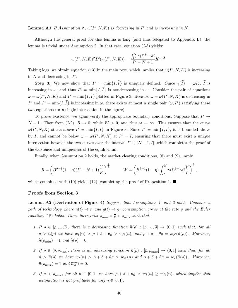
Lemma A1 If Assumption 2′

, ω(I∗, N,K) is decreasing in I∗ and is increasing in N .

Although the general proof for this lemma is long (and thus relegated to Appendix B), the

lemma is trivial under Assumption 2. In that case, equation (A5) yields:

ω(I∗, N,K)σLs(ω(I∗, N,K)) =

∫ NI∗ γ(i)

σ−1di

I∗ −N + 1K1−σ.

Taking logs, we obtain equation (13) in the main text, which implies that ω(I∗, N,K) is increasing

in N and decreasing in I∗.

Step 3: We now show that I∗ = min{I, I} is uniquely defined. Since γ(I) = ωK, I is

increasing in ω, and thus I∗ = min{I, I} is nondecreasing in ω. Consider the pair of equations

ω = ω(I∗, N,K) and I∗ = min{I, I} plotted in Figure 3. Because ω = ω(I∗, N,K) is decreasing in

I∗ and I∗ = min{I, I} is increasing in ω, there exists at most a single pair (ω, I∗) satisfying these

two equations (or a single intersection in the figure).

To prove existence, we again verify the appropriate boundary conditions. Suppose that I∗ →

N − 1. Then from (A2), R → 0, while W > 0, and thus ω → ∞. This ensures that the curve

ω(I∗, N,K) starts above I∗ = min{I, I} in Figure 3. Since I∗ = min{I, I}, it is bounded above

by I, and cannot be below ω = ω(I∗, N,K) at I∗ = I, ensuring that there must exist a unique

intersection between the two curves over the interval I∗ ∈ (N − 1, I], which completes the proof of

the existence and uniqueness of the equilibrium.

Finally, when Assumption 2 holds, the market clearing conditions, (8) and (9), imply

R =

(Bσ−1(1− η)(I∗ −N + 1)

Y

K

) 1σ

W =

(Bσ−1(1− η)

∫ N

I∗γ(i)σ−1di

Y

L

) 1σ

,

which combined with (10) yields (12), completing the proof of Proposition 1. �

Proofs from Section 3

Lemma A2 (Derivation of Figure 4) Suppose that Assumptions 1′ and 2 hold. Consider a

path of technology where n(t) → n and g(t) → g, consumption grows at the rate g and the Euler

equation (18) holds. Then, there exist ρmin < ρ < ρmax such that:

1. If ρ ∈ [ρmin, ρ], there is a decreasing function n(ρ) : [ρmin, ρ] → (0, 1] such that, for all

n > n(ρ) we have wI(n) > ρ + δ + θg > wN (n), and ρ + δ + θg = wN (n(ρ)). Moreover,

n(ρmin) = 1 and n(ρ) = 0.

2. If ρ ∈ [ρ, ρmax], there is an increasing function n(ρ) : [ρ, ρmax] → (0, 1] such that, for all

n > n(ρ) we have wI(n) > ρ + δ + θg > wN (n) and ρ + δ + θg = wI(n(ρ)). Moreover,

n(ρmax) = 1 and n(ρ) = 0.

3. If ρ > ρmax, for all n ∈ [0, 1] we have ρ + δ + θg > wI(n) ≥ wN (n), which implies that

automation is not profitable for any n ∈ [0, 1].

40

4. If ρ < ρmin, for all n ∈ [0, 1] we have wI(n) ≥ wN (n) > ρ + δ + θg, which implies that new

tasks do not increase aggregate output and will not be adopted for any n ∈ [0, 1].

Proof. Because consumption grows at the rate g and the Euler equation (18) holds, we have

R(t) = ρ+ δ + θg.

The effective wages wI(n) and wN (n) are then determined the ideal price index condition, (A4), as

B1−σ =(1− n)cu(ρ+ δ + θg)1−σ +

∫ n

0cu(wI(n)

γ(i)

)1−σ

di (A6)

=(1− n)cu(ρ+ δ + θg)1−σ +

∫ n

0cu(γ(i)wN (n))1−σdi.

Differentiating these expressions, we obtain

w′I(n)

wI(n)=

1

1− σ

(cu(ρ+ δ + θg)1−σ − cu(wN (n))1−σ

) 1∫ n0 c

u′

(wN (n)γ(i))cu(wN (n)γ(i))−σwN (n)γ(i)di

w′N (n)

wN (n)=

1

1− σ

(cu(ρ+ δ + θg)1−σ − cu(wI(n))

1−σ) 1∫ n

0 cu′

(wN (n)γ(i))cu(wN (n)γ(i))−σwN (n)γ(i)di.

(A7)

To prove part 1, define ρmin as

ρmin + δ + θg = wN (1),

and define ρ > ρmin as

cu(ρ+ δ + θg)1−σ = B1−σ.

(When Assumption 2 holds we get ρ = B − δ − θg, as claimed in the main text).

To show that ρ > ρmin, note that

1

1− σcu(ρmin + δ + θg)1−σ =

1

1− σ

∫ 1

0cu(ρmin + δ + θg)1−σdi

=1

1− σ

∫ 1

0cu(wN (1))1−σdi

<1

1− σ

∫ 1

0cu(wN (1)γ(i))1−σdi

=1

1− σB1−σ

=1

1− σcu(ρ+ δ + θg)1−σ .

Because the function 11−σ c

u(x)1−σ is increasing, we have ρ > ρmin.

Using the ideal price index condition, (A4), we define n(ρ) implicitly as

B1−σ = (1− n(ρ))cu(ρ+ δ + θg)1−σ +

∫ n(ρ)

0cu(γ(i)(ρ+ δ + θg))1−σdi.

41

Differentiating the above expression with respect to ρ shows that n(ρ) is decreasing. Moreover,

n(ρmin) = 1 and n(ρ) = 0, so the function is well-defined for ρ ∈ [ρmin, ρ].

For n = n(ρ), we have wI(n(ρ)) > ρ + δ + θg = wN (n(ρ)). Thus, the formulas for w′I(n) and

w′N (N) show that, for ρ ∈ [ρmin, ρ] and starting at n(ρ), the curve wN (n) decreases in n and the

curve wI(n) is increasing in n. Thus, for all n > n(ρ), we have

wI(n) > wI(n(ρ)) > ρ+ δ + θg = wN (n(ρ)) > wN (n),

as claimed. On the other hand, for all n < n(ρ), we have wN (n) > ρ+ δ + θg.

To prove part 2, define ρmax > ρ as

ρmax + δ + θg = wI(1).

To show that ρ < ρmax, a similar argument establishes

1

1− σcu(ρmax + δ + θg)1−σ =

1

1− σ

∫ 1

0cu(ρmax + δ + θg)1−σdi

>1

1− σ

∫ 1

0cu(wI(1)/γ(i))

1−σdi

=1

1− σcu(ρ+ δ + θg)1−σ .

Because the function 11−σ c

u(x)1−σ is increasing, we have ρ < ρmax.

Using (A6), we define the function n(ρ) implicitly as

B1−σ = (1− n(ρ))cu(ρ+ δ + θg)1−σ +

∫ n(ρ)

0cu((ρ+ δ + θg)/γ(i))1−σdi.

Differentiating this expression with respect to ρ shows that n(ρ) is increasing in ρ on [ρ, ρmax].

Moreover, n(ρmax) = 1 and n(ρ) = 0, so the function is well-defined for all ρ ≥ ρ.

For n = n(ρ), we have wI(n(ρ)) = ρ + δ + θg > wN (n(ρ)). Thus, the formulas for w′I(n) and

w′N (n) show that, for ρ ∈ [ρ, ρmax] and starting at n(ρ), the curve wN (n) decreases in n and the

curve wI(n) is increasing in n. Thus, for all n > n(ρ), we have

wI(n) > wI(n(ρ)) = ρ+ δ + θg > wN (n(ρ)) > wN (n),

as claimed. On the other hand, for all n < n(ρ), we have wI(n) < ρ + δ + θg. In this region we

have n∗ = n(ρ) > n, and not all automated tasks are produced with capital.

To prove part 3, note that for ρ > ρmax, we have

ρ+ δ + θg > wI(1) > wN (1).

The expressions for w′I(n) and w

′N (n) show that, in this region, as n decreases, so does wI(n). Thus

ρ+ δ+ θg > wI(n) > wN (n), and for all these values we have n∗ = 1, and no task will be produced

with capital.

42

To prove part 4 note that for ρ < ρmin, we have

ρ+ δ + θg < wN (1) < wI(1).

The expressions for w′I(n) and w

′N (N) show that, in this region, as n decreases, both wN (n) wN (n)

increase. Thus ρ + δ + θg < wN (n) < wI(n) and for these values of ρ new tasks do not raise

aggregate output.

Proof of Proposition 4: We prove this proposition under the more general Assumption 2′

.

We start by deriving necessary conditions on N(t) and I(t) such that the economy admits a

BGP, and then show that these are also sufficient for establishing the existence of a unique and

globally stable BGP.

The capital market clearing condition implies that:

cu(R(t))ζ−σR(t)−ζK(t)

Y (t)= (1− n∗(t)).

Because in a BGP the rental rate of capital, R(t), and the capital to aggregate output ratio, K(t)Y (t) ,

are constant, we must have n∗(t) = n, or in other words, labor and capital must perform a fixed

measure of tasks.

Lemma A2 shows that we have four possibilities corresponding to the four cases in Proposition

4, each of which we now discuss in turn.

1. All tasks are automated: n∗(t) = n = 0. Because in this case capital performs all

tasks, Lemma A2 implies that we must have ρ < ρ and I(t) = N(t). In this part of the parameter

space, net output is given by AKK, and the economy grows at the rate AK−δ−ρθ . The transversality

condition, (19), is satisfied if and only if AK − δ > AK−δ−ρθ —or r > g. Moreover, positive growth

imposes AK > δ + ρ. The (generalized version of the) ideal price index condition, equation (A4),

then implies that R = cu−1(B1−σ1−σ ), and thus AK = cu−1(B

1−σ1−σ ). Under Assumption 2, this last

expression further simplifies to AK = B as claimed in the text.

We now show that The necessary conditions in this case are sufficient to generate balanced

growth. Suppose ρ < ρ and I(t) = N(t) so that n∗(t) = 0. Because all tasks all tasks are

produced with capital, we also have FL = 0, and thus the representative household supplies zero

labor. Consequently, the dynamic equilibrium can be characterized as the solution to the system

of differential equations

C(t)

C(t)=1

θ(AK − δ − ρ)

K(t) =(AK − δ)K(t)− C(t)eν(0)θ−1θ ,

together with the initial condition, K(0) > 0 and the trasversality condition, (19). We next show

that there is a unique solution to the system, and this solution converges to the full automation

BGP described in the proposition.

Define c = CK . The behavior of c is governed by the differential equation,

˙c(t)

c(t)=

1

θ(AK − δ − ρ)− (AK − δ) + c(t)eν(0)

θ−1θ .

43

This differential equation has a stable rest point at zero and an unstable rest point at cB =(Ak − δ − 1

θ (AK − δ − ρ))eν(0)

1−θθ > 0. There are therefore three possible equilibrium paths for

c(t): (i) it immediately jumps to cB and stays there; (ii) it starts at [0, cB) and converges to zero;

(iii) it starts at (cB ,∞) and diverges. The second and third possibilities violate, respectively, the

transversality condition (19) (because the capital stock would grow at the rate Ak−δ, implying r =

g), and the resource constraint (when c(t) = ∞). The first possibility, on the other hand, satisfies

the transversality condition (since asymptotically it involves r > g), and yields an equilibrium path.

In this path the economy converges to a unique BGP in which C(t) and K(t) grow at a constant

rate AK−δ−ρθ , thus also establishing uniqueness and global stability.

2. Interior equilibrium in which automated tasks are immediately produced with

capital: n∗(t) = n(t) = n ∈ (0, 1). Because capital performs all automated tasks, Lemma A2

implies that n > max{n(ρ), n(ρ)} and N(t) = I(t). Moreover, because in this candidate BGP R(t)

is constant, the general form of the ideal price index condition, (A4), implies that W (t)/γ(I(t))

must be constant too, and this is only possible if I(t) = ∆. Consequently, the growth rate of

aggregate output is A∆. Finally, the transversality condition, (19), is satisfied given the condition

ρ + (θ − 1)A∆ > 0 in this part of the proposition. Lemma A2 then verifies that n∗(t) = n >

n(ρ). Substituting the market clearing conditions for capital and labor, (A2) and (A3), into (1),

(2) and (3) and then subtracting the costs of intermediates, we obtain net output as F (k, L;n).

(When Assumption 2 holds, F (k, L;n) is given by the CES aggregate in equation (16)). F (k, L;n)

exhibits constant returns to scale, and because factor markets are competitive, we also have R(t) =

FK(k(t), L(t);n) and w(t) = FL(k(t), L(t);n).

To establish uniqueness, let wB denote the BGP value of the wage rate, kB the BGP value of

the normalized capital stock, cB the BGP value of normalized consumption, LB the BGP value of

employment, and RB the BGP value of the rental rate of capital. These variables are, by definition,

all constant. Then, the Euler equation, (18), implies

RB = ρ+ δ + θg, and because RB = FK(kB , LB ;n), we must also have kBLB

= φ, where φ is the

unique solution to

FK(φ, 1;n) = ρ+ δ + θg.

Lemma B1 in Appendix B shows that, for n ≥ max{n(ρ), n(ρ)}, F (φ, 1;n) satisfies the following

Inada conditions,

limφ→0

FK(φ, 1;n) >ρ+ δ + θg limφ→∞

FK(φ, 1;n) <ρ+ δ + θg,

which ensure that φ is well defined. Combining labor supply condition, (17), with the resource

constraint, (20), we obtain (F (φ, 1;n)− (δ + g)φ)LB = FL(φ,1)ν′(LB) . The left-hand side of this equation

is linear and increasing in L (the concavity of F in k implies that F (φ, 1;n) > φFK(φ, 1;n) >

(δ+g)φ), while the right-hand side is decreasing in L. This ensures that there exists a unique value

LB > 0 that satisfies this equation, and also pins down the value of the normalized capital stock

as kB = φLB. Finally, cB is uniquely determined from the resource constraint, (20), as

cB = (F (φ, 1;n)− (δ + g)φ)LBeν(LB) 1−θ

θ .

44

Note also that there cannot be any BGP with LB = 0, since this would imply cB = 0 from the

resource constraint, (20). But then we would have ν′(0)eθ−1θ

ν(0) < FL(φ,1;n)cB

, which contradicts the

labor supply optimality condition, (17). Hence, the only possible BGP is one in which k(t) = kB ,

c(t) = cB and L(t) = LB > 0. Moreover, in view of the fact that ρ + (θ − 1)A∆ > 0, this

candidate BGP satisfies the transversality condition (19), and is indeed the unique BGP. The

proof of the global stability of this unique BGP is similar to the analysis of global stability of the

neoclassical growth model with endogenous labor supply, and for completeness, we provide the

details in Appendix B.

Interior equilibrium in which automated tasks are eventually but not immediately

produced with capital: n∗(t) = n(ρ) > n(t). Because capital does not immediately perform

all automated tasks, Lemma A2 implies that n(t) < n(ρ) and ρ > ρ. Moreover, because R(t) is

constant, the ideal price index condition, (A4), implies that W (t)/γ(I∗(t)) must be constant too.

Thus, to generate constant growth of wages we must have I∗(t) = ∆ ≤ I(t), so that the growth rate

of the economy is given by A∆. Because n∗(t) = n(ρ), this also implies that N∗(t) = ∆. Finally,

the transversality condition, (19), is satisfied in view of the fact that this part of the proposition

imposes ρ + (θ − 1)A∆ > 0. The uniqueness and global stability of the BGP follow an identical

arguments to part 2, with the only modification that n(ρ) plays the role of n in the preceding proof.

All tasks are always produced with labor: n∗(t) = 1. Because labor performs all tasks,

Lemma A2 now implies ρ > ρmin and n(t) ≥ 1, while the ideal price index condition, (A4), imposes

that W (t)/γ(N(t)) must be constant. Thus, to generate constant wage, aggregate output and

capital growth, we must have N(t) = ∆, with ρ + (θ − 1)∆ > 0 (where the last condition again

ensures transversality). To show sufficiency of these conditions for balanced growth, let wB denote

the BGP value of the normalized wage, which is defined by

∫ 1

0cu(wB/γ(i))

1−σ = B1−σ.

Consequently, net output is given by F (k, L;n) = wBγ(N(t) − 1)L(t), and thus depends linearly

on labor and is independent of capital. This implies K(t) = 0 and C(t) = wBγ(N(t)− 1)L(t). The

representative household’s labor supply condition, (17), implies that in this BGP

ν′(L(t)) =wBγ(N(t)− 1)

C(t)=

1

L(t),

which uniquely defines a BGP employment level LB. Because this allocation also satisfies the

transversality condition (in view of the fact that ρ+ (θ − 1)A∆ > 0), it defines a unique BGP. Its

global stability follows by noting that starting with any positive capital stock, K(0), the represen-

tative household chooses zero investment and converges to this path. �

Proofs from Section 4

All of the results in this section apply and will be proved, under Assumption 2′

.

45

Lemma A3 (Asymptotic behavior of the normalized value functions) Suppose that Assump-

tions 1′

, 2′

and 4. Let g = A κIκN

κI+κNS denote the growth rate of the economy in a BGP. Then there

exists a threshold S such that for S < S, we have that ρ+ (θ − 1)g > 0, and

• if n ≥ max{n, n}, both vN (n) and vI(n) are positive and increasing in n;

• if n ≤ n(ρ) (and ρ > ρ), we have κNvN (n) > κIvI(n) = O(g) (meaning that it goes to zero

as g → 0);

• If n < n(ρ) (and ρ < ρ), we have κIvI(n) > 0 > κNvN (n). Moreover, in this region, vI(n) is

decreasing and vN (n) is increasing in n.

Proof. See Appendix B.

Proof of Proposition 6: We first show that all the scenarios described in the proposition are

BGPs with endogenous technology. We then turn to analyzing the stability of interior BGPs.

Part 1: Characterization of the BGPs with endogenous technology.

Suppose that S < S so that Lemma A3 applies. We consider the two cases described in the

proposition separately.

1. ρ < ρ: Suppose that n < n(ρ). As depicted in the left panel of Figure 8 and shown in Lemma

A3, in this region vI(n) is positive and decreasing in n, and vN (n) is negative and increasing in

n. Thus, the only possible BGP in this region must be one with n(t) = 0. No interior BGP exists

with n ∈ (0, n(ρ)). Proposition 4 shows that for ρ < ρ, a path for technology with n(t) = 0 yields

balanced growth. Moreover, along this path all tasks are produced with capital, which implies that

VI(t) = VN (t) = 0. Thus, a path for technology in which n(t) = 0 is consistent with the equilibrium

allocation of scientists. The resulting BGP is an equilibrium with endogenous technology.

2. ρ > ρ: Suppose n(t) ≤ n(ρ). Then, we have n∗(t) = n(ρ) and therefore vN (n) = vN (n(ρ))

and vI(n) = vI(n(ρ)). Moreover, Lemma A3 implies that κNvN (n(ρ)) > κIvI(n(ρ)) and vI(n(ρ)) =

O(g) with g small (again because S < S). Therefore, in this region this region we always have that

all scientists will be employed to create new tasks, and thus n > 0 (and is uniformly bounded away

from zero). But this contradicts n(t) < n(ρ). Suppose, instead, that n(t) > n(ρ). Then, Proposition

4 shows that the economy admits a BGP only if n(t) = n. Thus, a necessary and sufficient

condition for an interior BGP is (29) in the text. Consequently, each interior BGP corresponds to

a solution to this equation in (n(ρ), 1). Lemma A3 shows that at n, κNvN (n) is above κIvI(n), and

κIvI(n) = O(g). Moreover, when κI

κN= 0, the entire curve κNvN (n) is above the curve κIvI(n). As

this ratio increases, the curve κIvI(n) rotates up, and eventually crosses κNvN (n) at a point to the

right of n(ρ). This defines the threshold κ. Above this threshold, there exists another threshold κ

such that if κI

κN> κ, there is a unique intersection of κIvI(n) and κNvN (n). (Note that one could

have κ = κ). By continuity, there exists S such that, the thresholds κ and κ are defined for all

S < S (recall that g = A κIκN

κI+κNS). It then follows that for S < min{S, S} and κI

κN> κ, there

exists a unique BGP, which is interior and satisfies n(t) = n∗(t) = nB ∈ (n, 1). For S < min{S, S}

and κ < κI

κN< κ (provided that κ < κ), the economy admits multiple BGPs with endogenous

46

technology. Finally, for S < min{S, S} and κI

κN< κ, the only potential BGP in this case is the

corner one with n(t) = 1, which we also described in Proposition 4. Because κNvN (1) > κIvI(1),

this path for technology is consistent with the equilibrium allocation of scientists and provides a

BGP with endogenous technology.

Part 2: Stability analysis.

The stability analysis applies to the case in which ρ > ρ, S < min{S, S} and κI

κN> κ. In this

case, the economy admits a unique BGP defined by nB ∈ (n(ρ), 1). We denote by cB , kB and LB

the values of (normalized) consumption and capital, and employment in this BGP.

Proof of global stability when θ = 0: Because θ = 0, we also have R = ρ + δ, and capital

adjusts immediately and its equilibrium stock only depends on n, which becomes the unique state

variable of the model.

Let v = κIvI −κNvN . Now starting from any n(0), an equilibrium with endogenous technology

is given by the path of (n, v) such that the evolution of the state variable is given by

n = κNS − (κN + κI)G (v)S;

and the evolution of the difference of the normalized value functions, v, satisfies the forward looking

equation:

ρv − v = bκI

(cu (ρ+ δ)ζ−σ − cu (wI)

ζ−σ)− bκN

(cu (wN )ζ−σ − cu (ρ+ δ)ζ−σ

)+O(g);

and in addition the transversality condition (19) holds.

When g = 0, the locus for v = 0 crosses zero from below at a unique point (recall that we are in

the parameter region where there is a unique BGP). By continuity there exists a threshold S such

that, for S < S, the locus for v = 0 crosses zero from below at a unique point nB , which denotes

the BGP value for n(t) derived from (29).

Figure A2: Phase diagram and global saddle path stability when θ = 0. The figure plots the locus for v = 0 and

the locus for n = 0. The unique BGP is located at their interception.

We now analyze the stability properties of the system and show that the BGP is globally saddle-

path stable. Figure A2 presents the phase diagram of the system in (v, n). The locus for v = 0

47

crosses v = 0 at nB from below only once. This follows from the fact that κIvI(n) cuts κNvN (n)

from below at nB as shown in Figure 8. The laws of motion of the two variables, v and n, take the

form shown in the phase diagram.31 This implies the existence of the unique stable arm, and also

establishes that there are no equilibrium paths that are not along this stable arm. In particular,

all paths above the stable arm feature v > 0 and eventually n → 0 and v → ∞, and since vN is

positive, vI → ∞. But this violates the transversality condition, (27). Similarly, all paths below

the stable arm feature v < 0 and eventually n → 1 and v → −∞, and thus vN → ∞, once again

violating the transversality condition.

Proof of local stability of the unique BGP when θ > 0: Appendix B shows that there

exists a threshold S such that the BGP in this case is locally stable for S < S, and thus the

conclusions of the proposition follow setting S = min{S, S, S, S}. �

References

Acemoglu, Daron (1998) “Why Do New Technologies Complement Skills? Directed Tech-

nical Change and Wage Inequality,” Quarterly Journal of Economics, 113(4): 1055-1089.

Acemoglu, Daron (2002) “Directed Technical Change,” Review of Economic Studies, 69(4):

781–810.

Acemoglu, Daron (2003) “Labor- and Capital-Augmenting Technical Change,” Journal of

European Economic Association, 1(1): 1–37.

Acemoglu, Daron (2007) “Equilibrium Bias of Technology,” Econometrica, 75(5): 1371–

1410.

Acemoglu, Daron (2010) “When Does Labor Scarcity Encourage Innovation?” Journal of

Political Economy, 118(6): 1037–1078.

Acemoglu, Daron and David Autor (2011) “Skills, tasks and technologies: Implications

for employment and earnings,” Handbook of Labor Economics, 4: 1043–1171.

Acemoglu, Daron, Gino Gancia and Fabrizio Zilibotti (2010) “Competing Engines of

Growth: Innovation and Standardization,” Journal of Economic Theory, 147(2): 570–601.

Acemoglu, Daron, Gino Gancia and Fabrizio Zilibotti (2015) “Offshoring and Directed

Technical Change,” forthcoming American Economic Journal: Macro.

Acemoglu, Daron and Fabrizio Zilibotti (2001) “Productivity Differences,” Quarterly

Journal of Economics, 116(2): 563–606.

Acemoglu, Daron and Pascual Restrepo (2017) “Robots and Jobs: Evidence from US

Labor Markets” NBER Working Paper No. 23285.

Aghion, Philippe and Peter Howitt (1992) “A Model of Growth Through Creative De-

struction,” Econometrica, 60(2): 323–351.

31This can also be verified locally from the fact that the behavior of n and v near the BGP can be approximated bythe linear system n = −(κN +κI)G

′(0)Sv and v = ρv−Q, where Q > 0 denotes the derivative of −MκIcu (wI)

ζ−σ +MκNc

u (wN )ζ−σ with respect to n (this derivative is positive because κIvI(n) cuts κNvN (n) from below at nB).Because the eigenvalues of the characteristic polynomial of this system add up to ρ > 0, and their product is−Q(κN + κI)G

′(0)S < 0, there is one positive and one negative eigenvalue.

48

Akst, Daniel (2013) “What Can We Learn From Past Anxiety Over Automation?” Wilson

Quarterly.

Allen, Robert C. (2009) “Engels’ Pause: Technical Change, Capital Accumulation, and

Inequality in the British Industrial Revolution,” Explorations in Economic History, 46(4): 418–

435.

Autor, David H. and David Dorn (2013) “The Growth of Low-Skill Service Jobs and the

Polarization of the U.S. Labor Market,” American Economic Review, 103(5): 1553–97.

Autor, David H., Frank Levy and Richard J. Murnane (2003) “The Skill Content of

Recent Technological Change: An Empirical Exploration,” The Quarterly Journal of Economics,

118(4): 1279–1333.

Beaudry, Paul, David A. Green, Benjamin M. Sand (2013) “The Great Reversal in the

Demand for Skill and Cognitive Tasks,” NBER Working Paper No. 18901.

Brynjolfsson, Erik and Andrew McAfee (2014) The Second Machine Age: Work, Progress,

and Prosperity in a Time of Brilliant Technologies, W. W. Norton & Company.

Burstein, Ariel, and Jonathan Vogel (2014) “International Trade, Technology, and the

Skill Premium,” Society for Economic Dynamics, Meeting Papers. No. 664.

Burstein, Ariel, Eduardo Morales and Jonathan Vogel (2014) “Accounting for Changes

in Between-Group Inequality,” NBER Working Paper No. 20855

Caselli, Francesco (1999) “Technological Revolutions,” American Economic Review, 89(1):

78–102.

Caselli, Francesco, and Wilbur John Coleman (2006) “The World Technology Frontier,”

American Economic Review, 96(3): 499–522.

Chandler, Alfred D. (1977) The Visible Hand: The Managerial Revolution in American

Business, Harvard University Press: Cambridge, MA.

Costinot, Arnaud and Jonathan Vogel (2010) “Matching and Inequality in the World

Economy,” Journal of Political Economy, 118(4): 747–786.

Foote, Christopher L. and Richard W. Ryan (2014) “Labor-Market Polarization Over

the Business Cycle,” NBER Macroeconomics Annual 2014, Volume 29, NBER.

Galor, Oded and Omer Moav (2000) “Ability-Biased Technological Transition, Wage In-

equality, and Economic Growth,” The Quarterly Journal of Economics, 115(2): 469–497.

Goldin, Claudia and Lawrence F. Katz (2008) The Race between Education and Tech-

nology, Harvard University Press: Cambridge.

Greenwood, Jeremy and Mehmet Yorukoglu (1997) “1974,” Carnegie-Rochester Con-

ference Series on Public Policy, 46: 49–95

Grossman, Gene M. and Elhanan Helpman (1991) “Quality Ladders in the Theory of

Growth,” The Review of Economic Studies, 58(1): 43–61.

Grossman, Gene M. and Esteban Rossi-Hansberg (2008) “Trading Tasks: A Simple

Theory of Offshoring,” American Economic Review, 98(5): 1978–1997.

49

Grossman, Gene M., Elhanan Helpman and Ezra Oberfield (2016) “Balanced Growth

Despite Uzawa,” NBER Working Paper No. 21861.

Hawkins, William, Ryan Michaels and Jiyoon Oh (2015) “The Joint Dynamics of

Capital and Employment at the Plant Level,” Mimeo, Yeshiva University.

Jaimovich, Nir and Henry E. Siu (2014) “The Trend is the Cycle: Job Polarization and

Jobless Recoveries,” NBER Working Paper No. 18334.

Keynes John Maynard (1930) “Economic Possibilities for Our Grandchildren,” in Essays

in Persuasion, New York: Norton & Co.

Kotlikoff, Laurence J. and Jeffrey D. Sachs (2012) “Smart Machines and Long Term

Misery,” NBER Working Paper No. 18629.

Jones, Charles I. (2005) “The Shape of Production Functions and the Direction of Technical

Change,” The Quarterly Journal of Economics, 120(2): 517–549.

Karabarbounis, Loukas and Brent Neiman (2014) “The Global Decline of the Labor

Share,” The Quarterly Journal of Economics, 129(1): 61–103.

Kiley, Michael T. (1999) “The Supply of Skilled Labor and Skill-Biased Technological

Progress,” The Economic Journal, 109(458): 708–724.

Landes, David (1969) The Unbound Prometheus, Cambridge University Press: New York.

Lin, Jeffrey (2011) “Technological Adaptation, Cities, and New Work” Review of Economics

and Statistics, 93(2): 554–574.

Mokyr, Joel (1990) The Lever of Riches: Technological Creativity and Economic Progress,

Oxford University Press: New York.

Nelson, Richard R. and Edmund S. Phelps (1966) “Investment in Humans, Technological

Diffusion, and Economic Growth,” The American Economic Review, 56(1): 69–75.

Oberfield, Ezra and Devesh Raval (2014) “Micro Data and Macro Technology,” NBER

Working Paper No. 20452.

Rodriguez-Clare, Andres (2010) “Offshoring in a Ricardian World,” American Economic

Journal: Macroeconomics, 2: 227–258.

Roy, A. D. (1951) “Some Thoughts on the Distribution of Earnings,” Oxford Economic

Papers, 3(2): 135–146.

Schultz, Theodore (1975) “The Value of the Ability to Deal with Disequalibria.” Journal

of Economic Literature. 13:827–846.

The New York Times (1983) “Machines vs. Workers,” by Charlotte Curtis, February 8th

edition.

Thoenig, Mathias, and Thierry Verdier (2003) “A Theory of Defensive Skill-Biased

Innovation and Globalization,” American Economic Review, 93(3): 709–728.

Zeira, Joseph (1998) “Workers, Machines, and Economic Growth,” Quarterly Journal of

Economics, 113(4): 1091–1117.

Zeira, Joseph (2006) “Machines as Engines of Growth,” Dynamics, Economic Growth, and

International Trade Conference Papers. No. 011059.

50

Appendix B (Not-For-Publication): Omitted Proofs and Additional

Results

Details of the Empirical Analysis

Here we provide information about the data used in constructing Figures 1 and 9. We also provide

a regression analysis documenting the robustness of the patterns illustrated in these figures.

Data: We use data on the demographic characteristics of workers and employment counts in

each of the 330 consistently defined occupations proposed by David Dorn (see http://www.ddorn.

net/data.htm). Our sources of data are the U.S. Censuses for 1980, 1990 and 2000, and the

American Community Survey for 2007. We focus on the set of workers between 16 and 64 years of

age.

Our measure of new job titles is taken from Lin (2011), who computes the share of new job

titles within each occupation for 1980, 1990 and 2000. Lin defines new job titles by comparing

changes across waves of the Dictionary of Occupational Titles, and also by comparing the 1990

Census Index of Occupations with its 2000 counterpart. The data is available for 329 occupa-

tions in 1980, and 330 occupations for 1990 and 2000. The data are available from his website

https://sites.google.com/site/jeffrlin/newwork.

Detailed Analysis for Figure 1: To document the role of new job titles in employment

growth, we estimate the regression

lnEit+10 − lnEit = βNit + δt + ΓtXit + εit. (B1)

Here, the dependent variable is the percent change in employment from year t to t + 10 in each

occupation i. We stack the data for t = 1980, 1990, 2000. For t = 2000, we use the change from

2000 to 2007 as the dependent variable and re-scale it to a 10-year change. In all regressions

we include a full set of decadal effects δt, and in some models we also control for differential

decadal trends that vary depending on observable characteristics of each occupation, ΓtXit. These

characteristics include the share of workers in different 5-year age brackets and from different races

(Black, Hispanic), and the share of foreign and female workers. These covariates flexibly control for

demographic changes that may affect the labor supply that is relevant for each occupation. Finally,

εit is an error term. Throughout, all standard errors are robust against arbitrary heteroskedasticity

and serial correlation of the error term within occupations.

The coefficient of interest is β, which represents the additional employment growth in occupa-

tions with a large share of new job titles, Nit.

Panel A in Table B1 presents estimates of equation (B1). Column 1 contains no additional

covariates (the number of observations in this column is 989. We miss one observation because

Lin’s measure only covers 329 occupations in 1980). Our estimates indicate that occupations with

10 percentage points more new job titles at the beginning of each decade grew 5.05% faster over the

decade (standard error= 1.29%). If occupations with more new job titles did not grow any faster

than the benchmark category with no novel jobs, employment growth from 1980 to 2007 would

B-1

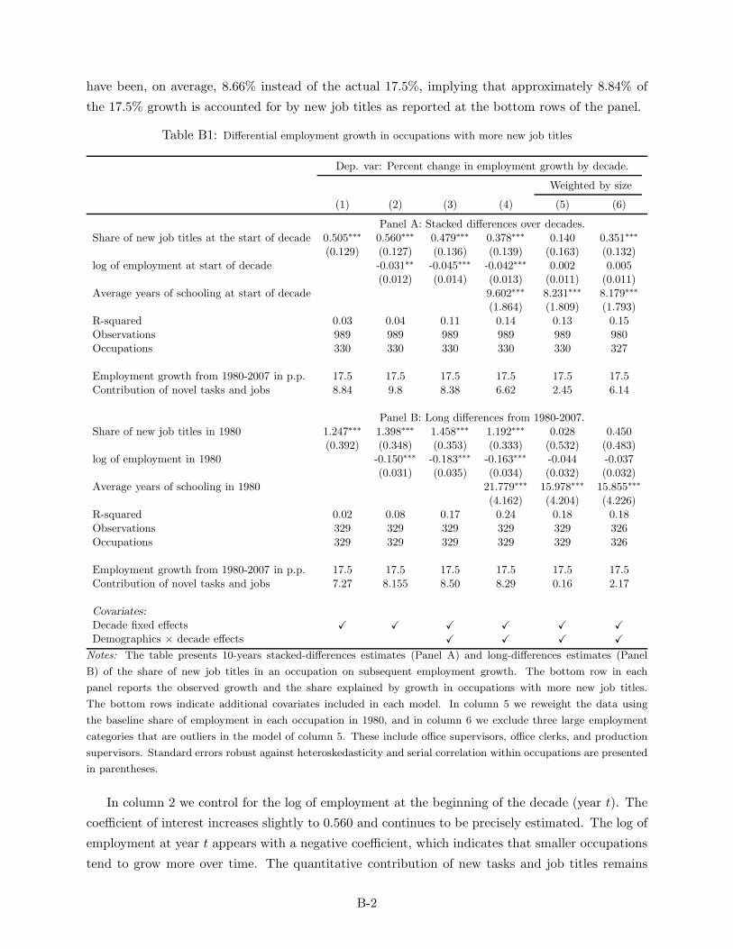
have been, on average, 8.66% instead of the actual 17.5%, implying that approximately 8.84% of

the 17.5% growth is accounted for by new job titles as reported at the bottom rows of the panel.

Table B1: Differential employment growth in occupations with more new job titles

Dep. var: Percent change in employment growth by decade.

Weighted by size

(1) (2) (3) (4) (5) (6)

Panel A: Stacked differences over decades.Share of new job titles at the start of decade 0.505∗∗∗ 0.560∗∗∗ 0.479∗∗∗ 0.378∗∗∗ 0.140 0.351∗∗∗

(0.129) (0.127) (0.136) (0.139) (0.163) (0.132)log of employment at start of decade -0.031∗∗ -0.045∗∗∗ -0.042∗∗∗ 0.002 0.005

(0.012) (0.014) (0.013) (0.011) (0.011)Average years of schooling at start of decade 9.602∗∗∗ 8.231∗∗∗ 8.179∗∗∗

(1.864) (1.809) (1.793)R-squared 0.03 0.04 0.11 0.14 0.13 0.15Observations 989 989 989 989 989 980Occupations 330 330 330 330 330 327

Employment growth from 1980-2007 in p.p. 17.5 17.5 17.5 17.5 17.5 17.5Contribution of novel tasks and jobs 8.84 9.8 8.38 6.62 2.45 6.14

Panel B: Long differences from 1980-2007.Share of new job titles in 1980 1.247∗∗∗ 1.398∗∗∗ 1.458∗∗∗ 1.192∗∗∗ 0.028 0.450

(0.392) (0.348) (0.353) (0.333) (0.532) (0.483)log of employment in 1980 -0.150∗∗∗ -0.183∗∗∗ -0.163∗∗∗ -0.044 -0.037

(0.031) (0.035) (0.034) (0.032) (0.032)Average years of schooling in 1980 21.779∗∗∗ 15.978∗∗∗ 15.855∗∗∗

(4.162) (4.204) (4.226)R-squared 0.02 0.08 0.17 0.24 0.18 0.18Observations 329 329 329 329 329 326Occupations 329 329 329 329 329 326

Employment growth from 1980-2007 in p.p. 17.5 17.5 17.5 17.5 17.5 17.5Contribution of novel tasks and jobs 7.27 8.155 8.50 8.29 0.16 2.17

Covariates:

Decade fixed effects X X X X X X

Demographics × decade effects X X X X

Notes: The table presents 10-years stacked-differences estimates (Panel A) and long-differences estimates (Panel

B) of the share of new job titles in an occupation on subsequent employment growth. The bottom row in each

panel reports the observed growth and the share explained by growth in occupations with more new job titles.

The bottom rows indicate additional covariates included in each model. In column 5 we reweight the data using

the baseline share of employment in each occupation in 1980, and in column 6 we exclude three large employment

categories that are outliers in the model of column 5. These include office supervisors, office clerks, and production

supervisors. Standard errors robust against heteroskedasticity and serial correlation within occupations are presented

in parentheses.

In column 2 we control for the log of employment at the beginning of the decade (year t). The

coefficient of interest increases slightly to 0.560 and continues to be precisely estimated. The log of

employment at year t appears with a negative coefficient, which indicates that smaller occupations

tend to grow more over time. The quantitative contribution of new tasks and job titles remains

B-2

very similar to column 1, increasing slightly to 9.8%.

In column 3 we control for the trends that depend on the demographic covariates described

above, which have little effect on the quantitative results. In column 4, we also control for the

average years of schooling among workers in each occupation at the beginning of the decade.

Although this covariate reduces the magnitude of the coefficient of the share of new job titles, our

estimate for β remains highly significant. The contribution of new job titles is now estimated at

6.62% out of the 17.5% growth between 1980 and 2007.

Column 5 repeats the specification of column 4, but this time we reweight the data by the 1980

share of employment in each occupation. This weakens the relationship of interest, and the share of

novel tasks and jobs is no longer statistically significant. However, this lack of significance is driven

by a few large occupations that are outliers in the estimated relationship. (In contrast, there are

no major outliers in the unweighted regressions reported in columns 1-4). These outliers include

office supervisors, office clerks, and production supervisors; three occupations that had combined

employment of about 4 million workers in 1980 and have been contracting since then. Though these

occupations introduced a significant number of new job titles in 1980, they shed a large amount

of workers in the subsequent years. In column 6, we exclude these three occupations from our

analysis, and obtain a similar pattern to that of column 4.

Finally, in Panel B, we present a set of regressions, which are analogous to those in the top

panel, but that focus on a long difference specification between 1980 and 2007. The overall patterns

are very similar, and now the contribution of novel tasks and new job titles to the 17.5% growth

in employment between 1980 and 2007 is between 7.27 and 8.5%.

Detailed Analysis for Figure 9: To document the presence of some amount of “standard-

ization” of occupations with greater new job titles,

∆Yit = βNit + δt + ΓtXit + εit. (B2)

Here, the dependent variable is the change in the average years of schooling among workers employed

in occupation i and measured over different time horizons (10 years, 20 years or 30 years). We

stack the data for t = 1980, 1990, 2000, but our sample becomes smaller as we measure the change

in average years of schooling over longer periods of time. We again use the ACS dayear 2007. The

covariates and independent variable are the same ones that we used in equation (B1).

Panel A in Table B2 presents estimates of equation (B2). Columns 1 and 2 present models

in which the dependent variable is the change in average years of education over a 10-year period

(hence, we get 989 observations for 330 occupations). Columns 3 and 4 focus on the change in

average years of education over a 20-year period. Columns 5 and 6 focus on the change in average

years of education over a 30-year period. In the models presented in the even columns we include

a full set of trends that are allowed to vary depending on the composition of employment in each

occupational category.

Our estimates indicate that, although occupations with more new job titles tend to hire more

skilled workers initially, this pattern slowly reverts over time. Figure 9 shows that, at the time of

B-3

Table B2: Reversal in skill content for occupations with more new job titles and in occupations that used to hire

more educated workers.

Dep. var: Change in average years of schooling.

Over 10 years Over 20 years Over 30 years

(1) (2) (3) (4) (5) (6)

Panel A: Change in occupations with new job titles.Share of new job titles at the start of decade -0.085 -0.103 -0.219 -0.203 -0.452∗∗ -0.411∗∗

(0.123) (0.118) (0.179) (0.173) (0.215) (0.176)R-squared 0.32 0.53 0.12 0.33 0.02 0.29Observations 989 989 659 659 329 329Occupations 330 330 330 330 329 329

Panel B: Change in occupations with more educated workers.Average years of education at the start of decade -0.030∗∗∗ -0.077∗∗∗ -0.028∗∗ -0.102∗∗∗ -0.083∗∗∗ -0.149∗∗∗

(0.006) (0.011) (0.013) (0.017) (0.016) (0.021)R-squared 0.36 0.59 0.14 0.41 0.17 0.43Observations 990 990 660 660 330 330Occupations 330 330 330 330 330 330Covariates:

Decade fixed effects X X X X X X

Demographics × decade effects X X X

Notes: The table presents OLS estimates that explain the change in average years of schooling among workers

employed in a given occupation. These changes are computed over 10 years (Columns 1 and 2), 20 years (Columns

3 and 4) and 30 years (Columns 5 and 6). In Panel A we explain the subsequent change in years of schooling

as a function of share of new job titles in each occupation at the start of the decade. In Panel B we explain the

subsequent change in years of schooling as a function of the years of schooling in each occupation at the start of

the decade. The bottom rows indicate additional covariates included in each model. Standard errors robust against

heteroskedasticity and serial correlation within occupations are presented in parentheses.

their introduction, occupations with 10 percentage points more new job titles hire workers with 0.35

more years of schooling). But our estimates in Column 6 of Table B2 show that this initial difference

in the skill requirements of workers slowly vanishes over time. 30 years after their introduction,

occupations with 10 percentage points more new job titles hire workers with 0.0411 fewer years of

education than the workers hired initially (standard error= 0.0176).

Relatedly, Panel B of the same table shows a similar pattern when we look at occupations

that start with greater average years of schooling at the beginning of a decade. In particular,

for each decade since 1980, employment growth has been faster in occupations with greater skill

requirements—as measured by the average years of education among employees at the start of each

decade (see Table B1). But estimating a version of (B2) with average years of schooling at the

beginning of the decade on the right-hand side, we find significant mean reversion. For example,

Column 6 shows that occupations that used to hire workers with one additional year of schooling

workers reduce their average years of schooling by 0.149 years relative to baseline after 30 years

(standard error=0.021).

Remaining Proofs from Section 2

We start by providing the proof of Lemma A1.

B-4

Proof of Lemma A1. Denote by W (I∗, N,K) and R(I∗, N,K) the wage and interest rate for

task thresholds I∗, N and a supply of capital K. W (I∗, N,K) and R(I∗, N,K) are given by the

intercept of the ideal price index condition in equation (A4) and the equation

Ls

(W

RK

)(I∗ −N + 1)cu(R)ζ−σR−ζ −K

∫ N

I∗γ(i)ζ−1cu

(W

γ(i)

)ζ−σ

W−ζdi = 0,

which can be derived from the market clearing conditions for capital and labor in equations (A2)

and (A3).Taking total derivatives of this equation with respect to I∗, N , we obtain

dN

(Lscu(r)ζ−σr−ζ +Kγ(N)ζ−1cu

(W

γ(N)

)ζ−σ

W−ζ

)− dI∗

(Lscu(r)ζ−σr−ζ +Kγ(I∗)ζ−1cu

(W

γ(I∗)

)ζ−σ

W−ζ

)

= (d lnW − d ln r)

(K

∫ N

I∗γ(i)ζ−1cu

(W

γ(i)

)ζ−σ

W−ζ [s(i)(σ − ζ) + ζ] di+ εLLs(I∗ −N + 1)cu(r)ζ−σr−ζ

)

+ d ln r

(K

∫ N

I∗γ(i)ζ−1cu

(W

γ(i)

)ζ−σ

W−ζ [(s(i)− sk)(σ − ζ)] di

).

Here, s(i) is the share of labor in the production of task i and sk is the share of capital in

tasks produced with capital. The last term in the above equation captures the non-homotheticity

introduced by the presence of intermediate goods. When (s(i)− sk)(σ−ζ) = 0, the demand system

is homothetic and the results outlined in Lemma A1 follow easily. These cases include the limits

when ζ → 1 (and s(i) = sk are constant) or η → 0 (and s(i) = sk = 1 are constant).

When (s(i)− sk)(σ− ζ) 6= 0, we also need to take into account the movements in the ideal price

curve in equation (A4) to determine the behavior of relative factor prices.Differentiation of (A4) gives:

dN1

1− σ

(cu (r)1−σ − cu

(W

γ(N)

)1−σ)

+ dI1

1− σ

(cu(

W

γ(I∗)

)1−σ

− cu (r)1−σ

)

=(d lnW − d ln r)

(∫ N

I∗s(i)cu

(W

γ(i)

)1−σ

di

)+ d ln r

((I∗ −N + 1)skc

u(r)1−σ +

∫ N

I∗s(i)cu

(W

γ(i)

)1−σ

di

),

which implies that we can solve for d lnW − d lnR as

(d lnW − d lnR)Θ = dNPN − dIPI ,

where:

Θ =

(K

∫ N

I∗γ(i)ζ−1cu

(W

γ(i)

)ζ−σ

W−ζ [s(i)(σ − ζ) + ζ] di+ εLLs(I∗ −N + 1)cu(r)ζ−σr−ζ

)

×

((I∗ −N + 1)skc

u(r)1−σ +

∫ N

I∗s(i)cu

(W

γ(i)

)1−σ

di

)

−

(∫ N

I∗s(i)cu

(W

γ(i)

)1−σ

di

)×

(K

∫ N

I∗γ(i)ζ−1cu

(W

γ(i)

)ζ−σ

W−ζ [(s(i)− sk)(σ − ζ)] di

),

PN =

(Lscu(r)ζ−σr−ζ +Kγ(N)ζ−1cu

(W

γ(N)

)ζ−σ

W−ζ

)

×

((I∗ −N + 1)skc

u(r)1−σ +

∫ N

I∗s(i)cu

(W

γ(i)

)1−σ

di

)

−1

1− σ

(cu (r)1−σ − cu

(W

γ(N)

)1−σ)

×

(K

∫ N

I∗γ(i)ζ−1cu

(W

γ(i)

)ζ−σ

W−ζ [(s(i)− sk)(σ − ζ)] di

),

B-5

PI =

(Lscu(r)ζ−σr−ζ +Kγ(I∗)ζ−1cu

(W

γ(I∗)

)ζ−σ

W−ζ

)

×

((I∗ −N + 1)skc

u(r)1−σ +

∫ N

I∗s(i)cu

(W

γ(i)

)1−σ

di

)

+1

1− σ

(cu(

W

γ(I∗)

)1−σ

− cu (r)1−σ

)×

(K

∫ N

I∗γ(i)ζ−1cu

(W

γ(i)

)ζ−σ

W−ζ [(s(i)− sk)(σ − ζ)] di

).

We now show that, under the conditions of Lemma A1, we have Θ, PN , PI > 0.

A sufficient condition for Θ > 0 is that:(K

∫ N

I∗γ(i)ζ−1cu

(W

γ(i)

)ζ−σ

W−ζ [s(i)(σ − ζ) + ζ] di

)×

(∫ N

I∗s(i)cu

(W

γ(i)

)1−σ

di

)

≥

(∫ N

I∗s(i)cu

(W

γ(i)

)1−σ

di

)×

(K

∫ N

I∗γ(i)ζ−1cu

(W

γ(i)

)ζ−σ

W−ζ [(s(i)− sk)(σ − ζ)] di

).

After canceling common terms on both sides of this inequality, it boils down to:

∫ N

I∗

γ(i)ζ−1cu(W

γ(i)

)ζ−σ

[s(i)(σ − ζ) + ζ] di ≥

∫ N

I∗

γ(i)ζ−1cu(W

γ(i)

)ζ−σ

[(s(i)− sk)(σ − ζ)] di.

This can be rewritten as:∫ N

I∗γ(i)ζ−1cu

(W

γ(i)

)ζ−σ

[s(i)(σ − ζ) + ζ − (s(i)− sk)(σ − ζ)] di ≥ 0.

The last inequality always holds because s(i)(σ− ζ)+ ζ − (s(i)− sk)(σ− ζ) = σsk + ζ(1− sk) > 0.

To determine the signs of PN and PI , we regroup terms as follows. First, we group the terms

that are multiplied by sk in the expression for PI . To guarantee that these terms add up to a

positive number, a sufficient condition is given by:

(Lscu(r)ζ−σr−ζ

)× (I∗ −N + 1)skc

u(r)1−σ

≥

∣∣∣∣∣σ − ζ

1− σ

(cu(

W

γ(I∗)

)1−σ

− cu (r)1−σ

)∣∣∣∣∣×(K

∫ N

I∗skγ(i)

ζ−1cu(W

γ(i)

)ζ−σ

W−ζdi

).

We can use equations (A2) and (A3) to cancel terms on both sides of the above inequality and

obtain the sufficient condition:

cu(R)1−σ ≥

∣∣∣∣∣σ − ζ

1− σ

(cu(

W

γ(I∗)

)1−σ

− cu (R)1−σ

)∣∣∣∣∣ . (B3)

Second, we group the terms that are multiplied by s(i) in the expression for PI . To guarantee

that these terms add up to a positive number, a sufficient condition is given by:(Kγ(I∗)ζ−1cu

(W

γ(I∗)

)ζ−σ

W−ζ

)×

(∫ N

I∗s(i)cu

(W

γ(i)

)1−σ

di

)

≥

∣∣∣∣∣σ − ζ

1− σ

(cu(

W

γ(I∗)

)1−σ

− cu (r)1−σ

)∣∣∣∣∣×(K

∫ N

I∗s(i)γ(i)ζ−1cu

(W

γ(i)

)ζ−σ

W−ζdi

).

B-6

After removing common terms and re-grouping, this condition becomes

∫ N

I∗s(i)W−ζ

(γ(I∗)ζ−1cu

(W

γ(I∗)

)ζ−σ

cu(

W

γ(i)

)1−σ

− γ(i)ζ−1cu(

W

γ(i)

)ζ−σ∣∣∣∣∣σ − ζ

1− σ

(cu(

W

γ(I∗)

)1−σ

− cu (R)1−σ

)∣∣∣∣∣

)≥ 0.

(B4)

We now show that, for this condition to hold, it suffices that

(γ(I∗)

γ(i)

)max{σ,ζ}−1

cu(W

γ(i)

)1−σ

≥

∣∣∣∣∣σ − ζ

1− σ

(cu(

W

γ(I∗)

)1−σ

− cu (R)1−σ

)∣∣∣∣∣ . (B5)

We first show this in the case in which σ > ζ. In this case, we have

cu(

W

γ(I∗)

)ζ−σ

≥ cu(W

γ(i)

)ζ−σ ( γ(i)

γ(I∗)

)ζ−σ

.

This follows from the fact thatcu(

Wγ(i)

)

cu(

Wγ(I∗)

) ≥γ(I∗)

γ(i),

an inequality which can be proven by straightforward differentiation of the function cu(x)/x, which

is decreasing.Plugging this in the inequality in equation (B4), we obtain the sufficient condition

∫ N

I∗s(i)W−ζγ(i)ζ−σ

(γ(I∗)σ−1cu

(W

γ(i)

)ζ−σ

cu(

W

γ(i)

)1−σ

− γ(i)σ−1cu(

W

γ(i)

)ζ−σ∣∣∣∣∣σ − ζ

1− σ

(cu(

W

γ(I∗)

)1−σ

− cu (R)1−σ

)∣∣∣∣∣

),

which holds provided that

(γ(I∗)

γ(i)

)σ−1

cu(W

γ(i)

)1−σ

≥

∣∣∣∣∣σ − ζ

1− σ

(cu(

W

γ(I∗)

)1−σ

− cu (R)1−σ

)∣∣∣∣∣ .

This inequality coincides with the condition in equation (B5), completing this step of the proof.

We now turn to the case ζ ≥ σ. Because the cost function is increasing we have:

cu(

W

γ(I∗)

)ζ−σ

≥ cu(W

γ(i)

)ζ−σ

Plugging this in the sufficient condition in equation (B4) yields:

∫ N

I∗s(i)W−ζ

(γ(I∗)ζ−1cu

(W

γ(i)

)ζ−σ

cu(

W

γ(i)

)1−σ

− γ(i)ζ−1cu(

W

γ(i)

)ζ−σ∣∣∣∣∣σ − ζ

1− σ

(cu(

W

γ(I∗)

)1−σ

− cu (R)1−σ

)∣∣∣∣∣

),

which holds provided that

(γ(I∗)

γ(i)

)ζ−1

cu(W

γ(i)

)1−σ

≥

∣∣∣∣∣σ − ζ

1− σ

(cu(

W

γ(I∗)

)1−σ

− cu (R)1−σ

)∣∣∣∣∣ ,

once again establishing the sufficiency of (B5).

B-7

Third, we group the terms that are multiplied by s(i) in the expression for PN . To guarantee

that these terms add up to a positive number, a sufficient condition is given by:(Kγ(N)ζ−1cu

(W

γ(N)

)ζ−σ

W−ζ

)×

(∫ N

I∗s(i)cu

(W

γ(i)

)1−σ

di

)

≥

∣∣∣∣∣σ − ζ

1− σ

(cu (r)1−σ − cu

(W

γ(N)

)1−σ)∣∣∣∣∣×

(K

∫ N

I∗s(i)γ(i)ζ−1cu

(W

γ(i)

)ζ−σ

W−ζdi

).

This condition can be rewritten as:

∫ N

I∗s(i)W−ζ

[cu(

W

γ(i)

)1−σ

γ(N)ζ−1cu(

W

γ(N)

)ζ−σ

−

∣∣∣∣∣σ − ζ

1− σ

(cu (R)1−σ − cu

(W

γ(N)

)1−σ)∣∣∣∣∣ γ(i)

ζ−1cu(

W

γ(i)

)ζ−σ]di ≥ 0.

In Step 1 of the proof of this proposition, we showed that x−ζcu(x)σ−ζ is decreasing in x. This

implies that γ(N)ζcu(

Wγ(N)

)ζ−σ> γ(i)ζcu

(Wγ(i)

)ζ−σ.

Therefore, a sufficient condition for the terms that are multiplied by s(i) in the expression forPN to add up to a positive number is

∫ N

I∗s(i)γ(i)ζ−1cu

(W

γ(i)

)ζ−σ

W−ζ ×

[γ(I)

γ(N)cu(

W

γ(i)

)1−σ

−

∣∣∣∣∣σ − ζ

1− σ

(cu (R)1−σ − cu

(W

γ(N)

)1−σ)∣∣∣∣∣

]di ≥ 0.

This expression implies that, to guarantee that these terms are positive, the following relationship

would be sufficient

γ(I)

γ(N)cu(W

γ(i)

)1−σ

≥

∣∣∣∣∣σ − ζ

1− σ

(cu (R)1−σ − cu

(W

γ(N)

)1−σ)∣∣∣∣∣ . (B6)

Fourth, and lastly, we group the terms that are multiplied by sK in the expression for PN . To

guarantee that these terms add up to a positive number, a sufficient condition is given by:

Lscu(r)ζ−σr−ζ × (I∗ −N + 1)skcu(r)1−σ

≥

∣∣∣∣∣σ − ζ

1− σ

(cu (r)1−σ − cu

(W

γ(N)

)1−σ)∣∣∣∣∣×

(K

∫ N

I∗skγ(i)

ζ−1cu(W

γ(i)

)ζ−σ

W−ζdi

).

Using the market clearing conditions for capital and labor in equations (A2) and (A3), we can

rewrite the sufficient condition as:

cu(R)1−σ ≥

∣∣∣∣∣σ − ζ

1− σ

(cu(

W

γ(N)

)1−σ

− cu (R)1−σ

)∣∣∣∣∣ . (B7)

To finalize the proof of the lemma, we use the fact that for any effective factor prices p1, p2 (the

price per effective unit of labor or capital at any given task), we have

∣∣∣∣σ − ζ

1− σ

(cu (p1)

1−σ − cu (p2)1−σ)∣∣∣∣ ≤ |σ − ζ|cu

(W

γ(N − 1)

)cu(

W

γ(N)

)−σ

. (B8)

This inequality follows because f(x) = 11−σx

1−σ is a concave function and the effective factor prices

satisfy p1, p2 ∈[

Wγ(N) ,

Wγ(N−1)

](recall that because K > K, we have that W

γ(N) < R. Likewise, the

definition of I∗ imposes that Wγ(N−1) > R).

B-8

Inequality (B8) then implies that to guarantee (B3), (B5), (B6) and (B7), the following would

suffice

cu(R)1−σ ≥|σ − ζ|cu(

W

γ(N − 1)

)cu(

W

γ(N)

)−σ

.

(γ(I∗)

γ(i)

)max{σ,ζ}−1

cu(W

γ(i)

)1−σ

≥|σ − ζ|cu(

W

γ(N − 1)

)cu(

W

γ(N)

)−σ

.

γ(I)

γ(N)cu(W

γ(i)

)1−σ

≥|σ − ζ|cu(

W

γ(N − 1)

)cu(

W

γ(N)

)−σ

.

These inequalities can be, in turn, rewritten as

cu(R)

cu(

Wγ(N−1)

)

cu(

Wγ(N)

)

cu(R)

σ

≥|σ − ζ|.

(γ(I∗)

γ(i)

)max{σ,ζ}−1

cu(

Wγ(i)

)

cu(

Wγ(N−1)

)

cu(

Wγ(N)

)

cu(

Wγ(i)

)

σ

≥|σ − ζ|.

γ(I)

γ(N)

cu(

Wγ(i)

)

cu(

Wγ(N−1)

)

cu(

Wγ(N)

)

cu(

Wγ(i)

)

σ

≥|σ − ζ|.

From the properties of unit cost functions, it follows that for all p ∈[

Wγ(N) ,

Wγ(N−1)

]we have

cu (p) ≥ cu(

Wγ(N−1)

)γ(N−1)γ(N) and cu

(W

γ(N)

)≥ cu (p) γ(N−1)

γ(N) . Using these properties, it follows that

the sufficient conditions above hold whenever(γ(N − 1)

γ(N)

)1+σ

≥|σ − ζ|

(γ(N − 1)

γ(N)

)max{σ,ζ}+σ

≥|σ − ζ|

(γ(N − 1)

γ(N)

)2+σ

≥|σ − ζ|.

The first inequality above ensures the sufficient conditions (B3) and (B7) simultaneously; the second

inequality above ensures the sufficient condition (B5); and the last inequality above ensures the

sufficient condition (B6)

Thus a sufficient condition for all three inequalities to hold is

(γ(N − 1)

γ(N)

)2+2σ+ζ

≥ |σ − ζ|,

which completes the proof of the Lemma.

We now turn to Proposition 2. We first provide a similar Proposition which applies in general.

We then specialize to Assumption 2 to derive a sharp characterization of the comparative statics.

In what follows, we let ∂ω∂I∗ ,

∂ω∂N and ∂ω

∂K denote the partial derivatives of the function ω(I∗, N,K)

with respect to its arguments.

B-9

Proposition B1 (Comparative statics in the general model) Suppose that Assumptions 1,

2′

and 3 hold. Let εL > 0 denote the elasticity of the labor supply schedule Ls(ω) with respect to ω;

let εγ = d lnγ(I)dI > 0 denote the semi-elasticity of the comparative advantage schedule.

• If I∗ = I < I—so that the allocation of tasks to factors is constrained by technology—then:

– the impact of technological change on relative factor prices is given by

d ln(W/R)

dI=d lnω

dI=

1

ω

∂ω

∂I∗< 0,

d ln(W/R)

dN=d lnω

dN=

1

ω

∂ω

∂N> 0

– the impact of capital on relative factor prices is given by

d ln(W/R)

d lnK=d lnω

d lnK+ 1 =

1 + εLσcons + εL

> 0,

where σcons ∈ (0,∞) is the elasticity of substitution between labor and capital that applies

when technology constraints the allocation of factors to tasks. This elasticity is given by

a weighted average of σ and ζ.

• If I∗ = I < I—so that tasks are allocated to factors in the unconstrained cost minimizing

fashion—then

– the impact of technological change on relative factor prices is given by

d ln(W/R)

dI=d lnω

dI= 0,

d ln(W/R)

dN=d lnω

dN=σcons + εLσfree + εL

1

ω

∂ω

∂N> 0 and

– the impact of capital on relative factor prices is given by

d ln(W/R)

d lnK=d lnω

d lnK+ 1 =

(1 + εL

σfree + εL

)> 0,

where

σfree = (σcons + εL)

(1−

1

ω

∂ω

∂I∗

)− εL > σ;

• In both parts of the proposition, the labor share and employment move in the same direction

as ω.

• Finally, when Assumption 2 holds, both parts of the proposition apply as stated, with the

additional difference that now we can explicitly compute the derivatives as

1

ω

∂ω

∂I∗=−

1

σ + εLΛI

1

ω

∂ω

∂N=−

1

σ + εLΛN ,

and the elasticities of substitution as:

σcons =σ σfree =σ +1

εγΛI .

B-10

Note: In this proposition, we do not explicitly treat the case in which I∗ = I = I in order

to save on space and notation, since in this case left and right derivatives with respect to I are

different.

Proof. We first establish the comparative statics of ω with respect to I, N and K when both

I∗ = I < I and I∗ = I < I.

Comparative statics for K: The curve I∗ = min{I, I} does not depend onK, all comparative

statics are entirely determined by the effect of capital on ω(I∗, N,K). An increase in K shifts up

the relative demand locus in Figure A1 (this does not affect the ideal price index condition, which

simplifies the analysis in this case), and thus increases W and reduces R . The impact on ω = WRK

depends on whether the initial effect on W/R has elasticity greater than one (since K is in the

denominator).

Notice that the function ω(I∗, N,K) already incorporates the equilibrium labor supply response.

To distinguish this supply response from the elasticity of substitution determined by factor de-

mands, we define ωL(I∗, N,K,L) as the static equilibrium for a fixed level of the labor supply

L.

The definition of σcons implies that ∂ωL

∂KKωL = 1

σcons− 1 and −∂ωL

∂LLωL = 1

σcons. Thus, when

I∗ = I < I, we have

d ln(W/R) = d lnω + 1 =

(1

σcons− 1

)d lnK −

1

σconsεLd lnω + d lnK =

1 + εLσcons + εL

d lnK,

where we have used the fact that ω(I∗, N,K) = ωL(I∗, N,K,Ls(ω)). This establishes the claims

about the comparative statics with respect to K when I∗ = I < I.

For the case where I∗ = I < I, we have that the change in K also changes the threshold task

I∗ = I. In particular, dI∗ = 1εγd lnω. Thus,

d ln(W/R) =1 + εL

σcons + εLd lnK+

1

ω

∂ω

∂I∗1

εγd ln(W/R) =

1 + εLσcons + εL

1

1− 1ω∂ω∂I

1εγ

d lnK =1 + εL

σfree + εLd lnK,

where we define σfree as in the proposition.

Comparative statics with respect to I: The relative demand locus ω = ω(I∗, N,K) does

not directly depend on I . Thus, the comparative statics are entirely determined by the effect of

changes in I on the I∗ = min{I, I} schedule depicted in Figure 3. When I∗ = I < I, small changes

in I have no effect as claimed in the proposition. Suppose next that I∗ = I < I . In this case,

an increase in I shifts the curve I∗ = min{I, I} to the right in Figure 3. Lemma A1 implies that

ω(I∗, N,K) is decreasing in I∗. Thus, the shift in I increases I∗ and reduces ω—as stated in the

proposition. Moreover, because I∗ = I, we have

d ln(W/R)

dI=d lnω

dI∗=

1

ω

∂ω

∂I∗< 0,

where ∂ω∂I∗ denotes the partial derivative of ω(I∗, N,K) with respect to I∗.

B-11

Comparative statics for N : From Lemma A1, changes in N only shift the relative demand

curve up in Figure 3. Hence, when I∗ = I < I, we have

d ln(W/R)

dN=d lnω

dN=

1

ω

∂ω

∂N> 0,

where ∂ω∂N denotes the partial derivative of ω(I∗, N,K) with respect to N .

Turning next to the case where I∗ = I < I, note that the threshold task is given by γ(I∗) = ωK.

Therefore, dI∗ = 1εγd lnω (where recall that εγ is the semi-elasticity of the γ function as defined in

the proposition). Therefore, d ln(W/R)dN = d lnω

dN , and we can compute this total derivative as claimed

in proposition:

d lnω

dN=

1

ω

∂ω

∂N+

1

ω

∂ω

∂I∗1

εγ

d lnω

dN=

1ω

∂ω∂N

1− 1ω

∂ω∂I∗

1εγ

=σ cons + εLσfree + εL

1

ω

∂ω

∂N.

To conclude the proposition, we specialize to the case in which Assumption 2 holds. The explicit

expressions for the partial derivative ∂ω∂I∗ ,

∂ω∂N and σ presented in the proposition follow directly

from differentiating equation (13) in the main text. Finally, the definition of σfree in the proposition

implies that, in this case:

σfree = (σ + εL)

(1−

1

ω

∂ω

∂I∗

)− εL = σ +

1

εγΛI ,

which proofs the claims in Proposition 2 in the main text.

Proof of Proposition 3: The formulas provided for d lnY |K,L in this proposition only apply

when Assumption 2 holds. Thus, we only prove this proposition for the particular model analyzed

in the main text.

We start by deriving the formulas for d ln Y |K,L in the case in which technology binds and

I∗ = I < I. To do so, we first consider a change in dN and totally differentiate equation (12) in

the main text. We get:

d lnY |K,L =B

(1− η)Y

[Y (1− η)

B

] 1σ 1

σ − 1

γ(N)σ−1

(∫ NI∗ γ(i)

σ−1di

L

) 1−σσ

−

(I∗ −N + 1

K

) 1−σσ

dN

=B

(1− η)Y

[Y (1− η)

B

] 1σ 1

σ − 1

γ(N)σ−1

(B1−σW σ

(1− η)Y

) 1−σσ

−

(B1−σRσ

(1− η)Y

) 1−σσ

dN

=Bσ−1 1

1− σ

(R1−σ −

(W

γ(N)

)1−σ)dN.

B-12

Likewise, following a change in dI∗ we get:

d lnY |K,L =B

(1− η)Y

[Y (1− η)

B

] 1σ 1

σ − 1

(I∗ −N + 1

K

) 1−σσ

− γ(I)σ−1

(∫ NI∗ γ(i)

σ−1di

L

) 1−σσ

dI

=B

(1− η)Y

[Y (1− η)

B

] 1σ 1

σ − 1

(B1−σRσ

(1− η)Y

)1−σσ

− γ(I)σ−1

(B1−σW σ

(1− η)Y

) 1−σσ

dI

=Bσ−1 1

1− σ

((W

γ(I)

)1−σ

−R1−σ

)dI.

We now derive the formulas for the impact of technology on factor prices. Let sL denote the

labor share in net output. Because WL+RK = (1− η)Y , we obtain:

sLd lnW + (1− sL)d lnR = d ln Y |K,L . (B9)

Moreover, Proposition 2 implies that

d lnW − d lnR =1

σ + εLΛNdN −

1

σ + εLΛIdI. (B10)

Solving the system of equations given by (B9) and (B10), we obtain the formulas for d lnW and

d lnR in the proposition.

Now, consider the case in which I∗ = I < I. In this case we have:

d lnY |K,L = Bσ−1 1

1− σ

(R1−σ −

(W

γ(N)

)1−σ)dN +Bσ−1 1

1− σ

(W

γ(I)

)1−σ

−R1−σ

dI∗

= Bσ−1 1

1− σ

(R1−σ −

(W

γ(N)

)1−σ)dN.

Thus, changes in I∗ do not affect aggregate output because the marginal firm at I is indifferent

between producing with capital or producing with labor. On the other hand, because I is not

binding, changes in I do not affect aggregate output.

We derive the formulas for the impact of technology on factor prices as before, with the difference

that now equation (B10) becomes

d lnW − d lnR =1

σfree + εLΛNdN.

�

Remaining Proofs from Section 3

We start by providing an additional lemma showing that, for a path of technology in which g(t) = g

and n > max{n, n(ρ)}, the resulting production function F (k, L;n) satisfies the Inada conditions

required in a BGP.

B-13

Lemma B1 (Inada conditions) Suppose that Assumptions 1′ and 2 hold. Consider a path of

technology in which n(t) → n and g(t) → g. Let F (k, L;n) denote net output introduced in the

proof of Proposition 4. If n ≥ maxn(ρ), n(ρ) we have F satisfies the Inada conditions:

limφ→0

FK(φ, 1;n) >ρ+ δ + θg limφ→∞

FK(φ, 1;n) <ρ+ δ + θg.

Proof. Let φ = kL . Let MPK(φ) = FK(φ, 1;n) and w(φ) = FL(φ, 1;n) denote the rental rate of

capital and the wage at this ratio, respectively.

When n ≥ maxn(ρ), n(ρ), these factor prices satisfy the system of equations given by the ratio

of the market clearing conditions (A2) and (A3),

φ =(1− n)cu(MPK(φ))ζ−σMPK(φ)−ζ

∫ n0 γ(i)

ζ−1cu(w(φ)/γ(i))ζ−σw(φ)−ζ,

coupled with the ideal price index condition in equation (A4), which we can rewrite succinctly as:

B1−σ = (1− n)cu(MPK(φ))1−σ +

∫ n

0cu(w(φ)/γ(i))1−σdi. (B11)

We start by considering the limit case in which φ = 0. The factor-demand equation requires

that either (i) MPK(φ) = ∞, or (ii) w(φ) = 0. In the first case, we have MPK(φ) > ρ + δ + θg

as claimed. In the second case we have:

cu(0) =

{0 if ζ ≥ 1cu0 if ζ < 1.

We show that in both cases MPK(0) > ρ+ δ + θg:

1. Suppose that ζ ≥ 1. For the ideal price index condition in (B11) to hold, we require 1 > σ

(otherwise the right-hand side diverges). Moreover, the ideal price index condition in (B11)

implies that MPK(0) is implicitly given by:

(1− n)cu(MPK(0))1−σ = B1−σ.

First, suppose that ρ ≤ ρ. We have that

cu(MPK(0))1−σ > (1− n)cu(MPK(0))1−σ = B1−σ = cu(ρ+ δ + θg)1−σ .

Here we have used the fact that n ≥ 0 and the definition of ρ introduced in Lemma A2.

Because 1 > σ, the above inequality implies MPK(0) > ρ+ δ + θg ≥ ρ+ δ + θg as claimed.

Finally, suppose that ρ > ρ. Because n ≥ n(ρ), we have:

(1− n(ρ))cu(MPK(0))1−σ ≥ (1− n)cu(MPK(0))1−σ

= B1−σ

= (1− n(ρ))cu(ρ+ δ + θg)1−σ +

∫ n(ρ)

0cu((ρ+ δ + θg)/γ(i))1−σdi

> (1− n(ρ))cu(ρ+ δ + θg)1−σ .

B-14

Here we have also used the definition of n(ρ) introduced in Lemma A2. Because 1 > σ, the

above inequality implies MPK(0) > ρ+ δ + θg as claimed.

2. Suppose that ζ < 1. We have that 0 < cu0 ≤ cu(x)∀x. The ideal price index condition in

(B11) implies that MPK(0) is implicitly given by:

(1− n)cu(MPK(0))1−σ + ncu01−σ = B1−σ.

When 1 > σ, we have the following series of inequalities:

(1− n(ρ))cu(MPK(0))1−σ + n(ρ)cu01−σ ≥ (1− n)cu(MPK(0))1−σ + ncu0

1−σ

= B1−σ

= (1− n(ρ))cu(ρ+ δ + θg)1−σ

+

∫ n(ρ)

0cu((ρ+ δ + θg)/γ(i))1−σdi

> (1− n(ρ))cu(ρ+ δ + θg)1−σ + n(ρ)cu01−σ.

Here, we have used the fact that n ≥ n(ρ) and 0 < cu0 ≤ cu(x)∀x, and the definition of n(ρ)

introduced in Lemma A2. Because 1 > σ, the above inequality implies MPK(0) > ρ+ δ+ θg

as claimed.

When 1 < σ, the previous inequalities are reversed, and we get:

(1− n(ρ))cu(MPK(0))1−σ + n(ρ)cu01−σ < (1− n(ρ))cu(ρ+ δ + θg)1−σ + n(ρ)cu0

1−σ.

Because 1 < σ, the above inequality implies MPK(0) > ρ+ δ + θg as claimed.

We next consider the limit case in which φ = ∞. With a slight abuse of notation, we define

MPK(∞) = limφ→∞MPK(φ) and w(∞) = limφ→∞w(φ). The factor-demand equation requires

that either (i) MPK(∞) = 0, or (ii) w(∞) = ∞. In the first case, MPK(∞) < ρ + δ + θg.

In the second case we have:

cu(0) =

{∞ if ζ ≥ 1cu∞ if ζ > 1.

We show that in both cases MPK(∞) < ρ+ δ + θg.

1. Suppose that ζ ≤ 1. For the ideal price index condition in (B11) to hold, we require σ > 1

(otherwise the right-hand side diverges). Moreover, the ideal price index condition in (B11)

implies that MPK(∞) is implicitly given by:

(1− n)cu(MPK(∞))1−σ = B1−σ.

First, suppose that ρ ≥ ρ. We have that

cu(MPK(∞))1−σ > (1− n)cu(MPK(∞))1−σ = B1−σ = cu(ρ+ δ + θg)1−σ .

B-15

Here we have used the fact that n ≥ 0 and the definition of ρ introduced in Lemma A2.

Because σ > 1, the above inequality implies MPK(∞) < ρ+ δ + θg ≤ ρ+ δ + θgas claimed.

Finally, suppose that ρ < ρ. Because n ≥ n(ρ), we have:

(1− n(ρ))cu(MPK(∞))1−σ ≥ (1− n)cu(MPK(∞))1−σ

= B1−σ

= (1− n(ρ))cu(ρ+ δ + θg)1−σ +

∫ n(ρ)

0cu((ρ+ δ + θg)γ(i))1−σdi

> (1− n(ρ))cu(ρ+ δ + θg)1−σ .

Here we have also used the definition of n(ρ) introduced in Lemma A2. Because σ > 1, the

above inequality implies MPK(∞) < ρ+ δ + θg as claimed.

2. Suppose that ζ > 1. We have that 0 < cu(x) ≤ cu∞∀x. The ideal price index condition in

(B11) implies that MPK(∞) is implicitly given by:

(1− n)cu(MPK(∞))1−σ + ncu∞1−σ = B1−σ.

When 1 > σ, we have the following series of inequalities:

(1− n(ρ))cu(MPK(∞))1−σ + n(ρ)cu∞1−σ ≤ (1− n)cu(MPK(∞))1−σ + ncu∞

1−σ

= B1−σ

= (1− n(ρ))cu(ρ+ δ + θg)1−σ

+

∫ n(ρ)

0cu((ρ+ δ + θg)γ(i))1−σdi

< (1− n(ρ))cu(ρ+ δ + θg)1−σ + n(ρ)cu∞1−σ.

Here, we have used the fact that n ≥ n(ρ) and 0 < cu(x) ≤ cu∞∀x, and the definition of n(ρ)

introduced in Lemma A2. Because 1 > σ, the above inequality impliesMPK(∞) < ρ+δ+θg

as claimed.

When 1 < σ, the previous inequalities are reversed, and we get:

(1− n(ρ))cu(MPK(∞))1−σ + n(ρ)cu∞1−σ > (1− n(ρ))cu(ρ+ δ + θg)1−σ + n(ρ)cu∞

1−σ.

Because 1 < σ, the above inequality implies MPK(∞) < ρ+ δ + θg as claimed.

Proof of Global Stability for Part 2 of Proposition 4: Here we provide the details of

global stability of the interior equilibrium where all automated tasks are immediately produced

with capital (part 2 of Proposition 4). In particular, we show that the BGP given by k(t) = kB ,

c(t) = cB and L(t) = LB is globally stable.

B-16

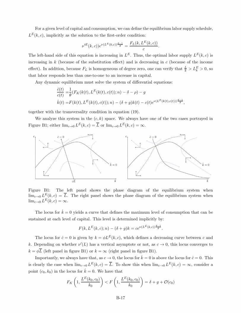
For a given level of capital and consumption, we can define the equilibrium labor supply schedule,

LE(k, c), implicitly as the solution to the first-order condition:

ν′E(k, c))eν(LE(k,c)) θ−1

θ =FL(k, L

E(k, c))

c.

The left-hand side of this equation is increasing in LE. Thus, the optimal labor supply LE(k, c) is

increasing in k (because of the substitution effect) and is decreasing in c (because of the income

effect). In addition, because FL is homogeneous of degree zero, one can verify that Lk > LE

k > 0, so

that labor responds less than one-to-one to an increase in capital.

Any dynamic equilibrium must solve the system of differential equations:

c(t)

c(t)=1

θ(FK(k(t), LE(k(t), c(t));n) − δ − ρ)− g

k(t) =F (k(t), LE(k(t), c(t));n) − (δ + g)k(t) − c(t)eν(LE(k(t),c(t))) θ−1

θ ,

together with the transversality condition in equation (19).

We analyze this system in the (c, k) space. We always have one of the two cases portrayed in

Figure B1; either limc→0 LE(k, c) = L or limc→0 L

E(k, c) = ∞.

Figure B1: The left panel shows the phase diagram of the equilibrium system whenlimc→0 L

E(k, c) = L. The right panel shows the phase diagram of the equilibrium system whenlimc→0 L

E(k, c) = ∞.

The locus for k = 0 yields a curve that defines the maximum level of consumption that can be

sustained at each level of capital. This level is determined implicitly by:

F (k, LE(k, c);n) − (δ + g)k = ceν(LE(k,c)) θ−1

θ .

The locus for c = 0 is given by k = φLE(k, c), which defines a decreasing curve between c and

k. Depending on whether ν′(L) has a vertical asymptote or not, as c → 0, this locus converges to

k = φL (left panel in figure B1) or k = ∞ (right panel in figure B1).

Importantly, we always have that, as c→ 0, the locus for k = 0 is above the locus for c = 0. This

is clearly the case when limc→0LE(k, c) = L. To show this when limc→0 L

E(k, c) = ∞, consider a

point (c0, k0) in the locus for k = 0. We have that

FK

(1,LE(k0, c0)

k0

)< F

(1,LE(k0, c0)

k0

)= δ + g +O(c0)

B-17

Thus, for c0 → 0, the condition ρ+ (θ − 1)g > 0 implies that

FK

(1,LE(k0, c0)

k0

)< ρ+ δ + θg.

This inequality implies that LE(k0,c0)k0

< φ, which is equivalent to the point (c0, k0) being in the

northeast region of the locus for c = 0.

As shown in Appendix A, both when limc→0 LE(k, c) = L or limc→0 L

E(k, c) = ∞, we have a

unique interior equilibrium at (cB , kB). Moreover, because as c→ 0 the locus for c = 0 is below the

locus for k = 0, we must have that the locus for c = 0 always cuts the locus for k = 0 from above

at (cB , kB). Thus, as shown in the phase diagrams in Figure B1 the unique interior equilibrium at

(cB , kB) is saddle-path stable.

One could also establish the saddle-path stability locally as follows. Around the interior BGP,

the system of differential equations that determines the equilibrium can be linearized as (suppressing

the arguments of the derivatives of the production function)

k(t) =

(ρ+ (θ − 1)g +

1

θFLL

Ek

)(k(t)− kB) +

(−eν(LB) θ−1

θ +1

θFLL

Ec

)(c(t) − cB)

c(t) =cBθ(FKK + FKLL

Ek )(k(t)− kB) +

cBθFKLL

Ec (c(t)− cB).

The characteristic matrix of the system is therefore given by

Mexog =

(ρ+ (θ − 1)g + 1

θFLLEk −eν(LB) θ−1

θ + 1θFLL

Ec

cBθ (FKK + FKLL

Ek )

cBθ FKLL

Ec

).

To analyze the properties of this matrix, we will use two facts: that FLLEK + cBFKLL

Ec = 0 and

FKK + FKLLEK < 0. The first fact follows by implicitly differentiating the optimality condition for

labor, which yields:

LEk =

1cFLk

eν(L)θ−1θ

(ν ′′(L) + θ−1

θ

)− 1

cFLL

LEc =−

1c2FL

eν(L)θ−1θ

(ν ′′(L) + θ−1

θ

)− 1

cFLL

.

The second fact follows by noting that, because LEK < LE

k , we have

FKK + FKLLEK < FKK + FKL

LE

k= 0.

Using these facts, we can compute the trace of Mexog:

Tr(Mexog) = ρ+ (θ − 1)g +1

θFLL

Ek +

cBθFKLL

Ec = ρ+ (θ − 1)g > 0.

In addition, the determinant of Mexog is given by:

Det(Mexog) =cBθFKLL

Ec

(ρ+ (θ − 1)g +

1

θFLL

Ek

)−cBθ(FKK + FKLL

Ek )

(1

θFLL

Ec − eν(LB) θ−1

θ

)< 0.

The inequality follows by noting that FKLLEc < 0 ρ + (θ − 1)g + 1

θFLLEk > 0 FKK + FKLL

Ek < 0

and 1θFLL

Ec − eν(L)

θ−1θ < 0.

B-18

(The negative determinant is equivalent to the fact established above that the curve for c = 0

cuts the curve for k = 0 from above. Moreover, the algebra here shows that, at the interception

point (cB , kB), the locus for k is increasing).

The sign of the trace and the determinant imply that the matrix has one positive and real

eigenvalue and one negative and real eigenvalue. Theorem 7.19 in Acemoglu (2009) shows that,

locally, the economy with exogenous technology is saddle-path stable as wanted.

To show the global stability of the unique BGP (cB , kB), all we need is to discard two types of

paths: the candidate paths that converge to zero capital, which we will show are not feasible, and

the candidate paths that converge to zero consumption, which we will show are not optimal.

To rule out the paths that converge to zero capital, note that all of them converge to an

allocation with k(t) = 0 and c(t) > c. Here c ≥ 0 is the maximum level of consumption that can

be sustained when k = 0, which is given by:

F (0, LE(0, c)) = ceν(LE(0,c)) θ−1

θ .

To rule out the paths that converge to zero consumption, we show that they violate the transver-

sality condition in equation (19). In all these paths we have c(t) → 0. There are two possible paths

for capital. Either capital converges to k—even at zero consumption the economy only sustains a

finite amount of capital—, or capital grows with no bound. In the first case, note that:

FK

(1,LE(k, c)

k

)≤ F

(1,LE(k, c)

k

)= δ + g.

Thus, the transversality condition in (19) does not hold. In the second case, we have that capital

grows at an asymptotic rate of F(1, L

E(k,c)k

)− δ− g. This is greater than or equal to the discount

rate used in the transversality condition in equation (19), which is FK

(1, L

E(k,c)k

)− δ − g. Thus,

the transversality condition does not hold in this case either. �

Proof of Proposition 5: We prove the proposition in the more general case in which As-

sumption 2’ holds.

Proposition 4 shows that for this path of technology the economy admits a unique BGP.

If n < n(ρ), we have that in the BGP n∗(t) = n(ρ) > n. Thus, small changes in n do not affect

the BGP equations; n does not affect effective wages, employment, or the labor share.

If n > n(ρ), we have that in the BGP n∗(t) = n. In this case, the behavior of the effective wages

follows from the formulas for w′I(n) and w

′N (N) in equation (A7), whose signs can be determined

given the ordering between wI(n), ρ+ δ + θg, and wN (n) derived in Lemma A2.

To characterize the behavior of employment, note that we can rewrite the first order condition

for the BGP level of employment in equation (17) as

1

Lν ′(L)=

c

wL=

1

sL

ρ+ (θ − 1)g

ρ+ δ + θg+

δ + g

ρ+ δ + θg.

It follows that, asymptotically, there is a positive relationship between employment and the labor

share. Thus, we can denote the BGP level of employment by an increasing function LLR(ω), whose

elasticity we denote by εLRL .

B-19

To characterize the behavior of the labor share we use Lemma A1. This lemma was derived for

the static model when the labor supply was given by Ls(ω), but we can use it here to describe the

asymptotic behavior of the economy when the supply of labor is given by LLR(ω) . In what follows

we use the same terminology employed in Proposition 2.

We consider two cases. First, suppose that σconst ≤ 1. Let kI(n) denote the BGP value for

K(t)/γ(I(t)). The definition of ω(I∗, N,K) implies that

ω(0, n, kI(n)) =wI(n)

(ρ+ δ + θg)kI (n).

Differentiating this expression, we obtain

k′I(n) =w′I(n)

1Rk − ∂ω

∂N

ωk

1+εLRL

σconst+εLRL

.

Using this expression for k′I(n), it follows that the total effect of technology on ω is given by

dω

dn=∂ω

∂N+∂ω

∂Kk′I(n)

=∂ω

∂N

(σconst + εLRL1 + εLRL

)+w′I(n)

Rk

(1− σconst

1 + εLRL

).

Because ∂ω∂N > 0 and w′

I(n) > 0, we have that, whenever σconst ≤ 1, ω is increasing in n. More-

over, because the BGP level of employment is given by the increasing function LLR(ω), n raises

employment too.

Next suppose that σconst > 1. Let kN (n) denote the BGP value forK(t)/γ(N(t)). The definition

of ω(I∗, N,K) implies that

ω(−n, 0, kN (n)) =wN (n)

(ρ+ δ + θg)kN (n).

Differentiating this expression, we have

k′N (n) =w′N (n) 1

Rk + ∂ω∂I∗

ωk

1+εLRL

σconst+εLRL

< 0.

Using this expression for k′N (n), it follows that the total effect of technology on ω is given by

dω

dn=−

∂ω

∂I∗+∂ω

∂Kk′N (n)

= −∂ω

∂I∗

(σ const + εLRL

1 + εLRL

)+w′N (n)

Rk

(1− σconst

1 + εLRL

).

Because ∂ω∂I∗ < 0 and w′

N (n) < 0, we have that, whenever σconst ≥ 1, ω is increasing in n. More-

over, because the BGP level of employment is given by the increasing function LLR(ω), n raises

employment too.

The previous observations show that automation reduces the labor share in the long run. In

addition, we have shown that k′N (n) < 0, which implies that in response to automation, capital

B-20

increases above its trend. The induced capital accumulation implies that the impact of automation

on the labor share worsens over time if σconst > 1 and eases if σconst < 1.

(When Assumption 2 holds the capital share is given by sK(t) = (1 − n)(R(t)B

)1−σ. In this

case, it follows trivially that n reduces the capital share and thus increases the labor share. This

expression also shows that, by bringing back the rental rate of capital to its BGP level, the induced

capital accumulation may worsen the decline in the labor share if σ > 1 or partially offset it if

σ < 1.) �

Remaining Proofs from Section 4

Proof of Lemma A3: In a BGP we have that the economy grows at the rate g = A κIκN

κI+κNS.

Suppose that n ≥ max{n, n}, we can write the value functions in the BGP as:

vN (n) = b

∫ ∞

0e−(ρ−(1−θ)g)τ

[cu (wN (n)egτ )ζ−σ − cu (ρ+ δ + θg)ζ−σ

]dτ ,

vI(n) = b

∫ ∞

0e−(ρ−(1−θ)g)τ

[cu (ρ+ δ + θg)ζ−σ − cu (wI(n)e

gτ )ζ−σ]dτ.

Thus, the value functions only depend on the unit cost of labor wN (n) and wI(n), and on the rental

rate, which is equal to ρ+ δ + θg in the BGP.

Now consider Taylor expansions of both of these expressions (which are continuously differen-

tiable) around S = 0—so that the growth rate of the economy is small:

vN (n) =b

ρ

[cu (wN (n))ζ−σ − cu (ρ+ δ + θg)ζ−σ

]+O(g), (B12)

vI(n) =b

ρ

[cu (ρ+ δ + θg)ζ−σ − cu (wI(n))

ζ−σ]+O(g).

Because O(g) → 0 as S → 0, we can approximate the above integrals when S is small with the

explicit expressions evaluated at g = 0.

Differentiating the value functions in (B12) establishes that they are both strictly increasing in

n. This follows from the result established in Proposition 5 that, in this region, wI(n) increases in

n and wN (n) decreases in n. Moreover, as S → 0 we find that both vN (n) and vI(n) are positive.

Thus, there exists S1 such that for S < S1, both vN (n) and vI(n) are positive ans strictly increasing

in n.

Now suppose that n ≤ n(ρ) (this case requires that ρ > ρ). In this region we have n∗(t) = n

and therefore vN (n) = vN (n) and vI(n) = vI(n). The value of automating a task is given by:

vI(n) = vI(n)

= b

∫ ∞

0e−(ρ−(1−θ)g)τ

[cu (ρ+ δ + θg)ζ−σ − cu (min{wI(n(ρ))γ(n− n(ρ))egτ , ρ+ δ + θg})ζ−σ

]dτ.

= b

∫ ∞

0e−(ρ−(1−θ)g)τ

[cu (ρ+ δ + θg)ζ−σ − cu ((ρ+ δ + θg)min{γ(n− n(ρ))egτ , 1})ζ−σ

]dτ.

The min operator min{wI(n(ρ))γ(n− n(ρ))egτ , ρ+ δ+ θg} shows that a task that is automated at

time t will only generate profits in the future starting at a time τ > t such that I∗(τ ) = I(t). At

B-21

this point in time, wI(n)γ(n − n(ρ))egτ = ρ + δ + θg, and it becomes profitable to use capital to

produce the automated task.

Because limg→0 vI(n) = 0, we have vI(n) = O(g). On the other hand, we have vN (n) = vN (n)

and this value function remains bounded away from zero as S → 0 . Thus, there exists S2 > 0 such

that for S < S2 , κNvN (n) > κIvI(n) > 0 as claimed, and vI(n) = O(g).

Finally, consider the case in which n < n(ρ) (this case requires that ρ < ρ). Because wN (n)egτ >

ρ+ δ+ θg and wI(n)egτ > ρ+ δ+ θg for all τ ≥ 0, it follows that, in this region, vI(n) > 0 > vN (n)

as claimed. Moreover, the derivatives for wI(n) and wN (n) in equation (A7) imply that, in this

region, both wI(n) and wN (n) are decreasing in n. Thus, in this region, vI(n) is decreasing and

vN (n) is increasing in n.

To finalize the proof of the Lemma we simply take S = min{S1, S2} if θ ≥ 1, and S =

min{S1, S2,ρ(κI+κN )

(1−θ)AκIκN} if θ < 1. This choice also ensures that ρ + (θ − 1)g > 0 as required in

the Lemma. �

Proof of local stability for the unique BGP when θ > 0: The local stability analysis

applies to the case in which ρ > ρ, S < min{S, S} and κI

κN> κ. In this case, the economy admits

a unique BGP.

An equilibrium is given by a solution to the following system of differential equations: Starting

from any n(0), k(0) the equilibrium with endogenous technology can be summarized by paths for

{c(t), k(t), n(t), v(t), SI (t)} such that:

1. The normalized consumption satisfies the Euler equation:

c

c=

1

θ(FK(k, L;n)− δ − ρ) +O(g).

2. The endogenous labor supply is given by LE(k, c;n), and is defined implicitly by:

cν ′ν(L)θ−1θ ≥ FL(k, L;n),

with equality if LE(k, c;n) > 0.

3. Capital satisfies the resource constraint:

k = F (k, L;n) +X(k, L;n) − δk − ceν(L)θ−1θ +O(g).

Here, X(k, L;n) = b(1 − n∗)ycu(FK)ζ−σ + by∫ n∗

0 cu(

FL

γ(i)

)ζ−σdi are the profits from the

intermediate sales.

4. Households face the transversality condition:

limt→∞

(k(t) + π(t))e−∫ t

0FK(k(s),L(s);n(s))−δ−O(g))ds = 0,

where π(t) = I(t)vI(t) +N(t)vN (t) are (the normalized) corporate profits.

B-22

5. Technology evolves endogenously according to:

n = κNS − (κI + κN )G(v)S.

6. The value function, v = κIvI − κNvN , satisfies

(FK − δ − g)v − v = bκIπI(k, L;n)− bκNπN (k, L;n) +O(g).

Around g = 0, the above system of differential equations is Lipschitz continuous (on their right-

hand side, the equations for c, k, n and v have bounded derivatives around the BGP {cB , kB , nB , vB}.

This can be seen from the matrix containing these derivatives Mendog, which we present below).

Thus, from the theorem of the continuous dependence of trajectories of a dynamical system on

parameters (e.g., Walter, 1998, page 146, Theorem VI), there exists a neighborhood of g = 0 and

a threshold S1 such that, for S < S1, the trajectories that solve the above system have the same

direction as the trajectories of the system evaluated at g = 0. In particular, for S < S1, the BGP

is locally saddle-path stable if and only if it is also locally saddle path stable in the limit in which

g = 0.

The previous argument shows that, to analyze the local stability of the BGP when S < S1, it

is enough to analyze the limit case in which g = 0. Thus, in what follows we focus on this limit.

As in the proof of Proposition 4, the Euler equation and the resource constraint can be linearized

around the BGP (denoted with the subscript B) as follows:

c =cBθ(FKn + FKLL

En )(n− nB) +

cBθFKLL

Ec (c− cB) +

cBθ(FKK + FKLL

Ek )(k − kB)

k =

(Fn +

1

θFLL

En +Xn +XLL

En

)(n− nB) +

(1

θFLL

Ec − eν(L)

θ−1θ +XLL

Ec

)(c− cB)

+

(FK +

1

θFLL

Ek − δ +Xk +XLL

Ek

)(k − kB).

Here, XK ,XL,Xn are the partial derivatives of X(k, L;n) with respect to each of its arguments.

Moreover, we have XK ,XL > 0—that is, the demand for intermediates increases with K and L.

We show that this property holds under Assumption 4, which imposes that σ > ζ, and ensures that

capital and labor are complements to intermediates. We first show this for L. We can rewrite X as

X =b

Bσ−1(1 − η)kRζ + by

∫ n

0cu(FL

γ(i)

)ζ−σ

di.

Thus:

XL =b

Bσ−1(1− η)kζRζ−1FKL

+MyL

∫ n

0cu(FL

γ(i)

)ζ−σ

di+ (ζ − σ)by

∫ n

0cu(FL

γ(i)

)ζ−σ

sL(i)FLL

FLdi > 0.

Here, sL(i) is the share of labor in the production of task i. The above inequality follows from the

fact that yL > 0, FKL > 0, and FLL < 0 (recall that Assumption 4 requires σ > ζ).

B-23

To show that XK > 0 we first differentiate the labor market clearing condition:

yky

=(σ − ζ)

∫ n0 c

u(

FL

γ(i)

)ζ−σγ(i)ζ−1sL(i)

FKL

FLdi

∫ n0 c

u(

FL

γ(i)

)ζ−σγ(i)ζ−1di

+ ζFLk

FL

>(σ − ζ)

∫ n0 c

u(

FL

γ(i)

)ζ−σγ(i)ζ−1sL(i)

FKL

FLdi

∫ n0 c

u(

FL

γ(i)

)ζ−σγ(i)ζ−1di

>(σ − ζ)

∫ n0 c

u(

FL

γ(i)

)ζ−σsL(i)

FKL

FLdi

∫ n0 c

u(

FL

γ(i)

)ζ−σdi

. (B13)

The last line in inequality (B13) follows from Chebyshev’s sum inequality, which applies here

because both γ(i)ζ−1 and sL(i) are increasing in i (when ζ > 1) or both are decreasing in i (when

ζ < 1).

Now, we have

XK =b(1− n)ykcu(FK)ζ−σ + (ζ − σ)b(1 − n∗)ycu(FK)ζ−σ sk

FKK

FK

+ byk

∫ n

0cu(FL

γ(i)

)ζ−σ

di+ by(ζ − σ)

∫ n

0cu(FL

γ(i)

)ζ−σ

sL(i)FLk

FLdi > 0.

Here sk is the share of capital in the production of automated tasks. The inequality follows from

the fact that yK > 0, FKK < 0 (recall that σ > ζ under Assumption 4), and the inequality in

equation (B13) derived above.

(When Assumption 2 holds, we have X = η1−ηF (k, L;n). In this case, it is clear that XK ,XL >

0).

In addition, let Qn, Qk, Qc > 0 denote the change in the incentives to automate (vs the incentives

to introduce new tasks) as n, k, c increase. All of these are positive.

The matrix that determines the local stability of the system is given by Mendog =

0 −(κI + κN )G′(0)S 0 0−Qn ρ −Qc −Qk

c∗

θ (FKn + FKLLEn ) 0 c∗

θ FKLLEc

c∗

θ (FKK + FKLLEk )

Fn + 1θFLL

En +Xn +XLL

En 0 1

θFLLEc − eν(L)

θ−1θ +XLL

Ec ρ+ 1

θFLLEk +Xk +XLL

Ek

.

The eigenvalues of this matrix (λ1, λ2, λ3, λ4) satisfy the following properties:

• The trace satisfies:

Tr(Mendog) = λ1 + λ2 + λ3 + λ4 = 2ρ+Xk +XLLEk > 0.

The last inequality follows from the fact that XL, LEk > 0

B-24

• The determinant satisfies:

Det(Mendog) =λ(κI + κN )G′(0)S×[cBθ

(1

θFLL

Ec − eν(L)

θ−1θ +XLL

Ec

)(Qn(FKK + FKLL

Ek )−Qk(FKn + FKLL

En ))

+cBθ

(ρ+

1

θFLL

Ek +Xk +XLL

Ek

)(Qc(FKn + FKLL

En )−QnFKLL

Ec

)

+cBθ

(Fn +

1

θFLL

En +Xn +XLL

En

)(QkFKLL

Ec −Qc(FKK + FKLL

Ek )).

The expression for the determinant can be further simplified by noting that Qc(FKK +

FKLLEk ) = QkFKLL

Ec . To show this, note that the impact of k, c on Q—the relative in-

centives for automation—depends on the ratio k/LE(k, c;n). For a given value of n, this

ratio determines factor prices and hence Q. Let φ = kLE(k,c;n)

. Then:

Qk =Qφ

(1

L−

k

L2LEk

)Qc =−Qφ

k

L2LEc .

These equations imply:

Qc = −QkkLE

c

L− kLEK

= QkFKLLEc

1kLE

k−L

k FKL

= QkFKLLEc

1

FKK + FKLLEk

,

which gives the desired identity.

Replacing this expression for Qc in the determinant, we get

Det(Mendog) =λ(κI + κN )G′(0)S×[cBθ

(1

θFLL

Ec − eν(L)

θ−1θ +XLL

Ec

)(Qn(FKK + FKLL

Ek )−Qk(FKn + FKLL

En ))

+cBθFKLL

Ec

(ρ+

1

θFLL

Ek +Xk +XLL

Ek

)(Qk

FKn + FKLLEn

FKK + FKLLEk

−Qn

).

Because we are focusing on a BGP in which, asymptotically, κIvI(n) intercepts κNvN (n) from

below, we have

Qn −QkFKn + FKLL

En

FKK + FKLLEk

> 0.

(Note that this is equivalent to the derivative of the profit function Q with respect to n when the

capital adjusts to keep the interest rate constant. This derivative is positive precisely when κIvI(n)

intercepts κNvN (n) from below). Because FKK+FKLLEk < 0 (as shown in the proof of Proposition

4), we also have that

Qn(FKK + FKLLEk )−Qk(FKn + FKLL

En ) < 0.

Thus, both terms in the determinant are positive and Det(Mendog) > 0 (recall that LEc < 0 and

LEk > 0, and XL,XK > 0).

B-25

Let Z(Mendog) = λ1λ2λ3 + λ2λ3λ4 + λ3λ4λ1 + λ4λ1λ2. We also have that

Z(Mendog) =ρDet(Mexog) +O(S).

Because Det(Mexog) < 0 and this determinant does not depend on S, we have that there exists a

S2 such that, for S < S2 we have that Z(Mendog) < 0.

We now show that the matrix has exactly two eigenvalues with negative real parts for S < S2.

Descarte’s rule of signs shows that the matrix has 0 or 2 positive real eigenvalues.

Suppose that the matrix has two positive real eigenvalues, p1, p2 > 0. Suppose to obtain a

contradiction that the remaining eigenvalues are complex and have a real part. Let z and its

conjugate z denote the eigenvalues. We then have:

S(Mendog) = 2ℜ(z)p1p2 + |z|2(p1 + p2) > 0,

a contradiction. Thus, in this case, exactly two eigenvalues have a negative real part.

Now suppose that the matrix has no positive real eigenvalues. Then we have two possible cases.

First, we could have that the eigenvalues are all complex and given by λ1, λ2 and their conjugates

λ1, λ2. We then have:

Z(Mendog) = 2ℜ(λ1)|λ2|+ 2ℜ(λ2)|λ1| < 0.

Thus, at least one of λ1 or λ2 has a negative real part. Moreover, exactly one of them has a negative

real part because

Tr(Mendog) = 2ℜ(λ1) + 2ℜ(λ2) > 0.

Second, we could have that the matrix has two negative real eigenvalues and a complex pair, λ and

λ. In this case, because the trace is positive, the real part of λ must be positive as well.

These observations show that when S < S2, Mendog has exactly two eigenvalues with negative

real parts. Thus, Theorem 7.19 in Acemoglu (2009) shows that, in the limit case in which g → 0

the economy with endogenous technology is saddle-path stable. Let S = min{S1, S2}. Thus, for

S < S, the unique BGP is locally stable. �

Proofs from Section 5

Proof of Proposition 7: We prove this proposition under Assumption 2 only. Consider an

exogenous path for technology in which N = I = ∆ (with ρ+ (θ − 1)AH∆ > 0) and suppose that

n(t) > max{n(ρ), n(ρ)}. This implies that in any candidate BGP I∗(t) = I(t) and n∗(t) = n(t).

Define M ∈ [I,N ] as in the main text. Two equations determine M . First, because firms are

indifferent between producing task M with low-skill or high-skill workers, we have:

WH(t)

WL(t)=

γH(M(t))

γL(M(t), t)=

γH(M(t))1−ξ

Γ(t− T (M(t))).

In addition, the relative demand for high-skill and low-skill labor yields:

L

H

∫ N(t)M(t) γH(i)σ−1di

∫M(t)I(t) γL(i, t)

σ−1di=

(WH(t)

WL(t)

)σ

.

B-26

These two equations can be combined into the equilibrium condition:

L

H

∫ N(t)M(t) γH(i)σ−1di

∫M(t)I(t) γL(i, t)

σ−1di=

(γH(M(t))1−ξ

Γ(t− T (M(t)))

)σ

.

Let m(t) = M(t) − I(t) and n = N(t) − I(t). Using the formula for γL(i, t) and the change of

variables i = N − i′ to rewrite the integrals in the previous equations we get that m(t) is uniquely

pinned down by:

L

H

∫ n−m(t)0 γH(i)1−σdi

∫ nn−m(t) γH(i)ξ(1−σ)Γ

(i∆

)σ−1di

=γH(N(t))1−ξ

γH(n−m(t))σ(1−ξ)Γ(n−m(t)

∆

)σ . (B14)

This expression also uses the fact that, because both N = I = ∆, we have t − T (i) = N(t)−i∆ .

The left-hand side of equation (B14)—the relative demand curve—is decreasing in m(t), converges

to zero as m(t) → n, and converges to infinity as m(t) → 0. Moreover, the right-hand side—the

comparative advantage schedule—is increasing in m(t). Thus, this equation uniquely determines

m(t) as a function of N(t) and n.

To prove the first part of the proposition, consider the case in which ξ < 1. Taking the limit

as t → ∞ we have that the right-hand side of equation (B14) converges to infinity. To maintain

the equality, we must have m(t) → 0, which implies that asymptotically M(t) = I(t) and low-skill

workers produce no task. Moreover, we have that inequality explodes, since

WH(t)

WL(t)→

γH(N(t))1−ξ

γ(n)1−ξΓ(n∆

) → ∞.

To prove the second part of the proposition, consider the case in which ξ = 1. We now show

that there is a BGP in which m(t) = m and WH (t)WL(t)

is constant. Equation (B14) shows that, in this

case, m only depends on n as claimed. Moreover, the wage gap is also constant over time and given

byWH(t)

WL(t)=

1

Γ(n−m∆

) .

Now, consider an increase in n, and let s = n −m denote the measure of tasks performed by

high-skill workers. Holding s constant, the left-hand side of equation (B14) is decreasing in n.

Because the left-hand side of equation (B14) is increasing in s and the right-hand side of equation

(B14) is decreasing in s, we must have that s increases as a result. This implies that, as stated in

the proposition, the wage gap, which is a decreasing function of s, declines with n. �

Proof of Proposition 8:

We prove this proposition in the more general case in which Assumption 2′ holds.

From the Bellman equations provided in the main text, it follows that along a BGP we have

vN (n) = b

∫ n∆

0e−(ρ−(1−θ)g)τ cu (wN (n)egτ )ζ−σ dτ ,

vI(n) = b

∫ 1−n∆

0e−(ρ−(1−θ)g)τ cu (ρ+ δ + θg)ζ−σ dτ.

B-27

Here ∆ = κIκN ι(nD)κI ι(nD)+κN

S is the endogenous rate at which both technologies grow in a BGP and

g = A∆.

As before, a BGP requires that n satisfies

κIι(n)vI(n) = κNvN (n).

Using these formulas, the proof of the proposition follows from the properties of the effective wages

derived in Proposition 5. Following the same steps involved in the proof of Proposition 6, we also

obtain that the equilibrium in this case is locally stable whenever κIι(n)vI(n) cuts κNvN (n) from

below. �

We now turn to Proposition 9. We prove a similar statement in the more general case in which

Assumption 2′ holds. In particular, we show that:

Proposition B2 (Welfare implications of automation in the general model) Consider the

static economy and suppose that Assumptions 1, 2′ and 3 hold, and that I∗ = I > I. Let

W = u(C,L) denote the welfare of households and let F (K,L; I,N) denote the resulting replace

when the amount of labor supplied is L and capital is K.

1. Consider the baseline model without labor market frictions, so that the representative house-

hold chooses the amount of labor without constraints, and thus WC = ν ′(L). Then:

dW

dI=(Ce−ν(L)

)1−θ FI

F> 0,

dW

dN=(Ce−ν(L)

)1−θ FN

F> 0.

2. Suppose that there are labor market frictions, so that employment is constrained by a quasi-

labor supply curve L ≤ Lqs(ω). Suppose also that the quasi-labor supply schedule Lqs(ω) is

increasing in ω, has an elasticity εL > 0, and is binding in the sense that WC > ν′(L). Then:

dW

dI=(Ce−ν(L)

)1−θ[FI

F− L

(W

C− ν ′(L)

)εLω

∂ω

∂I∗

]≶ 0.

dW

dN=(Ce−ν(L)

)1−θ[FN

F+ L

(W

C− ν′(L)

)εLω

∂ω

∂N

]> 0.

Proof. The unconstrained allocation of employment maximizes:

W = maxL

u(F (K,L; I,N), L).

Thus, the envelope theorem implies that:

WI = uCFI =(Ce−ν(L)

)1−θ FI

F> 0.

(recall that FI > 0 because we assumed I∗ = I).

B-28

Likewise, the envelope theorem implies that:

WN = uCFN =(Ce−ν(L)

)1−θ FN

F> 0.

(recall that FN > 0 because we imposed Assumption 3).

Now suppose that L ≤ Lqs(ω). The allocation of employment now solves:

W = maxL

u(F (K,L; I,N), L) + λ(Lqs(ω)− L),

where λ = ucFL + uL = cuc

(FL

c − ν′(L))> 0 is the multiplier on the employment constraint (by

assumption this constraint is binding). The envelope theorem now implies:

WI = uCFI + λL′qs(ω)

∂ω

∂I∗=(Ce−ν(L)

)1−θ[FI

F− L

(W

C− ν ′(L)

)εLω

∂ω

∂I∗

]≶ 0.

Likewise,

WN = uCFN + λL′qs(ω)

∂ω

∂N=(Ce−ν(L)

)1−θ[FI

F− L

(W

C− ν′(L)

)εLω

∂ω

∂N

]> 0.

The explicit formulas presented in Proposition 9 follow from the formulas presented here, but

using the fact that, when Assumption 2 holds, we have:

FI

F=Bσ−1

1− σ

((W

γ(I)

)1−σ

−R1−σ

)εLω

∂ω

∂I=

εLσ + εL

ΛI

FN

F=Bσ−1

1− σ

(R1−σ −

(W

γ(N)

)1−σ)

εLω

∂ω

∂N=

εLσ + εL

ΛN .

Properties of the constraint efficient allocation:

We now derive the constrained efficient allocation both when the labor market is frictionless

and when there is a friction as the one introduced in Proposition 9. We focus on the case in which

Assumption 2 holds, although similar insights apply in general.

First the planner removes markups. This implies that net output is given by

F p(K,L; I∗, N) =µη

η−1B

(I∗ −N + 1)

1σK

σ−1σ +

(∫ N

I∗γ(i)σ−1di

) 1σ

Lσ−1σ

σσ−1

,

= µη

η−1F (K,L; I∗, N).

Using this expression, we can write the planner’s problem as:

maxC(t),L(t),S(t)

∫ ∞

0e−ρt [C(t)e−ν(L(t))]1−θ − 1

1− θdt

Subject to

K(t) = µη

η−1F (K,L; I∗, N)− δK(t)− C(t).

B-29

Let µN (t) denote the marginal value of new tasks (increasing N) in terms of the final good.

Let µI(t) denote the marginal value of automation (increasing I) in terms of the final good. These

marginal values are the social counterparts to VN (t) and VI(t) in the decentralized economy. As-

suming that the planner operates in the region where I∗(t) = I(t), we can write these marginal

values as

µN (t) =(1− η)µη(1−σ)

∫ ∞

te−∫ τ

t(R(s)−δ)ds σ

1− σY (τ)

(R(τ)1−σ − γ(n(τ))σ−1w(τ )1−σ

)dτ ,

µI(t) =(1− η)µη(1−σ)

∫ ∞

te−∫ τ

t(R(s)−δ)ds σ

1− σY (τ)

(w(τ )1−σ −R(τ )1−σ

)dτ .

With some abuse of notation and to maximize the parallel with the decentralized expressions for

VN and VI , we are using R(t) to denote the marginal product of capital µη

η−1FK and w(t) to denote

the (normalized) marginal product of labor µη

η−1FLe−AI∗(t).

These observations show that the efficient allocation satisfies similar conditions to the decen-

tralized economy in our main model in Section 4. The only difference is that now, the allocation

of scientists is guided by µN (t) and µI(t) and satisfies:

SI(t) = SG

(κIµI(t)− κNµN (t)

Y (t)

), SN (t) = S

[1−G

(κIµI(t)− κNµN (t)

Y (t)

)],

so that in the efficient allocation, n(t) changes endogenously according to:

n(t) = κNS − (κN + κI)G

(κIµI(t)− κNµN (t)

Y (t)

)S.

One of the key insights from Proposition 6 is that the expected path for factor prices determines

the incentives to automate and create new tasks. The equations for µN and µI show that a planner

would also allocate scientists to developing both types of technologies following a similar principle;

guided by the cost savings that each technology grants to firms. However, the fact that µN 6= VN

and µI 6= VI shows that the decentralized allocation is not necessarily efficient. The inefficiency

arises because technology monopolists do not earn the full gains that their technology generates,

nor internalize how their innovations affect other existing and future technology monopolists.

We now show that labor market frictions change the planner’s incentives to allocate scientists.

By contrast, conditional on the wage level, such frictions do not change the market incentives to

automate or create new tasks.

Without frictions, the efficient level of labor satisfies

(µ

ηη−1FL − cν ′(L)

)µK ≤ 0,

with equality if L > 0.

Now suppose that there is an exogenous constraint on labor that requires L ≤ Lqs(ω). Let µL

be the multiplier of this constraint. We have that:

µL =

{ (µ

ηη−1FL − cν ′(L)

)µK > 0 if L = Lqs(ω)

0 if L < Lqs(ω)

B-30

Because the planner takes into account the first-order effects from changes in the employment level,

the values for µN and µI change to:

µN (t) = (1− η)µη(1−σ)

∫ ∞

te−∫ τ

t(R(s)−δ)ds

[σ

1− σY (τ)

(R(τ)1−σ − γ(n(τ))σ−1w(τ )1−σ

)

+(µ

ηη−1FL − cν ′(L)

)L

εLσ + εL

ΛN

]dτ,

µI(t) = (1− η)µη(1−σ)

∫ ∞

te−∫ τt(R(s)−δ)ds

[σ

1− σY (τ)

(w(τ )1−σ −R(τ )1−σ

)

−(µ

ηη−1FL − cν ′(L)

)L

εLσ + εL

ΛI

]dτ .

Thus, when the level of employment is below its unconstrained optimum, the planner values the

introduction of new tasks more because they raise the marginal product of labor and ease the

constraint on total employment. Likewise, the planner values automation less because she recognizes

that by reducing employment automation has a first-order cost on workers. Importantly, the market

does not recognize the first-order costs from automation or the first-order benefits from introducing

new tasks. As the expressions for VN and VI show, only factor prices—not the extent of frictions

in the labor market— determine the incentives to introduce these technologies.

When New Tasks Also Use Capital

In our baseline model, new tasks use only labor. This simplifying assumption facilitated our

analysis, but is not crucial or even important for our results. Here we outline a version of the

model where new tasks also use capital and show that all of our results continue to hold in this

case. Suppose, in particular, that the production function for non-automated tasks is

y(i) =

[ηq(i)

ζ−1ζ + (1− η)

(Bν(γ(i)l(i))

νk(i)1−ν) ζ−1

ζ

] ζζ−1

, (B15)

where k(i) is the capital used in the production of the task, ν ∈ (0, 1), and Bν = ν−ν(1− ν)−(1−ν)

is a constant that is re-scaled to simplify the algebra.

Automated tasks i ≤ I can be produced using labor or capital, and their production function

takes the form

y(i) =

[ηq(i)

ζ−1ζ + (1− η)

(k(i) +Bν(γ(i)l(i))

νk(i)1−ν) ζ−1

ζ

] ζζ−1

. (B16)

Comparing these production functions to those in our baseline model (2) and (3), we readily see

that the only difference is the requirement that labor has to be combined with capital in all tasks

(while automated tasks continue not to use any labor). Note also that when ν → 1, we recover

the model in the main text as a special case. It can be shown using a very similar analysis to

that in our main model that most of the results continue to hold with minimal modifications. For

example, there will exist a threshold I such that tasks below I∗ = min{I, I} will be produced

using capital and the remaining more complex tasks will be produced using labor. Specifically,

B-31

whenever R ∈ argmin{R,R1−ν

(Wγ(i)

)ν}and i ≤ I, the relevant task is produced using capital,

and otherwise it is produced using labor. Since γ(i) is strictly increasing, this implies that there

exists a threshold I at which, if technologically feasible, firms would be indifferent between using

capital and labor. Namely, at task I, we have R =W/γ(I), or

W

R= γ(I).

This threshold represents the index up to which using capital to produce a task yields the cost-

minimizing allocation of factors. However, if I > I, firms will not be able to use capital all the way

up to task I because of the constraint imposed by the available automation technology. For this

reason, the equilibrium threshold below which tasks are produced using capital is given by

I∗ = min{I, I},

meaning that I∗ = I < I when it is technologically feasible to produce task I with capital, and

I∗ = I < I otherwise.

The demand curves for capital and labor are similar, with the only modification that the demand

for capital also comes from non-automated tasks. Following the same steps as in the text, we

can then establish analogous results. This requires the more demanding Assumption 2′′, which

guarantees that the demand for factors is homothetic:

Assumption 2′′: One of the following three conditions holds:

1. σ − ζ → 0, or

2. ζ → 1, or

3. η → 0.

The following proposition is very similar to Proposition 1, with the only difference being in the

ideal price condition.

Proposition B3 (Equilibrium in the static model when ǫ ∈ (0, 1)) Suppose that Assumption

1′′ holds. Then, for any range of tasks [N−1, N ], automation technology I ∈ (N−1, N ], and capital

stock K, there exists a unique equilibrium characterized by factor prices, W and R, and threshold

tasks, I and I∗, such that: (i) I is determined by equation (6) and I∗ = min{I, I}; (ii) all tasks

i ≤ I∗ are produced using capital and all tasks i > I∗ are produced using labor; (iii) the capital and

labor market clearing conditions, equations (8) and (9), are satisfied; and (iv) factor prices satisfy

the ideal price index condition:

(I∗ −N + 1)cu(R)1−σ +

∫ N

I∗cu(R1−ν

(W

γ(i)

)ν)1−σ

di = 1. (B17)

B-32

Proof. The proof follows the same steps as Proposition 1.

Comparative statics in this case are also identical to those in the baseline model (as summarized

in Proposition 2) and we omit them to avoid repetition. The dynamic extension of this more general

model is also very similar, and in fact, Proposition 4 applies identically, and is also omitted. One

can also define ρ, n(ρ) and n(ρ) in an analogous nway as we did in the proof of Lemma A2. To

highlight the parallels, we just present the equivalent of Proposition 6.

Proposition B4 (Equilibrium with endogenous technology when ν ∈ (0, 1)) Suppose that

Assumptions 1′, 2′′, and 4 hold. Then, there exists S such that, when S < S, we have:

1 (Full automation) For ρ < ρ, there is a BGP in which n(t) = 0 and all tasks are produced

with capital.

For ρ > ρ, all BGPs feature n(t) = n > n(ρ). Moreover, there exist κ > κ > 0 such that:

2 (Unique interior BGP) if κI

κN> κ there exists a unique BGP. In this BGP we have

n(t) = n ∈ (n(ρ), 1) and κNvN (n) = κIvI(n). If, in addition, θ = 0, then the equilibrium is

unique everywhere and the BGP is globally (saddle-path) stable. If θ > 0, then the equilibrium

is unique in the neighborhood of the BGP and is asymptotically (saddle-path) stable;

3 (Multiple BGPs) if κ > κI

κN> κ, there are multiple BGPs;

4 (No automation) If κ > κI

κN, there exists a unique BGP. In this BGP n(t) = 1 and all tasks

are produced with labor.

Proof. The proof of this result closely follows that of Proposition 6, especially exploiting the fact

that the behavior of profits of automation and the creation of new tasks behave identically to those

in the baseline model, and thus the value functions behave identically also.

Microfoundations for the Quasi-Labor Supply Function

We provide various micro-foundations for the quasi-labor supply expression used in the main text,

Ls(

WRK

).

Efficiency wages: Our first micro-foundation relies on an efficiency wage story. Suppose that,

when a firm hires a worker to perform a task, the worker could shirk and, instead of working, use

her time and effort to divert resources away from the firm.

Each firm monitors its employees, but it is only able to detect those who shirk at the flow rate q

. If the worker is caught shirking, the firm does not pay wages and retains its resources. Otherwise,

the worker earns her wage and a fraction of the resources that she diverted away from the firm.

In particular, assume that each firm holds a sum RK of liquid assets that the worker could

divert, and that if uncaught, a worker who shirks earns a fraction u(i) of this income. We assume

that the sum of money that the worker may be able to divert is RK to simplify the algebra. In

B-33

general, we obtain a similar quasi-supply curve for labor so long as these funds are proportional to

total income Y = R K +WL.

In this formulation, u(i) measures how untrustworthy worker i is, and we assume that this

information is observed by firms. u(i) is distributed with support [0,∞) and has a cumulative

density function G. Moreover, we assume there is a mass L of workers. A worker of type u(i) does

not shirk if and only if:

W ≥ (1− q)[W + u(i)RK] →W

RK

q

1− q≥ u(i).

Thus, when the market wage is W , firms can only afford to hire workers who are sufficiently

trustworthy. The employment level is therefore given by:

Ls = G

(W

RK

q

1− q

)L.

When q = 1—so that there is no monitoring problem—, we have G(

WRK

q1−q

)= 1, and the supply

of labor is fixed at L for all wages W ≥ 0. However, when q < 1—so that there is a monitoring

problem—, we have Ls < L. Even though all workers would rather work than stay unemployed,

the monitoring problem implies that not all of them can be hired at the market wage. Notice that,

though it is privately too costly to hire workers with u(i) > WRK

q1−q , these workers strictly prefer

employment to unemployment.

Alternatively, one could also have a case in which firms do not observe u(i), which is private

information. This also requires that firms do not learn about workers. To achieve that, we assume

that workers draw a new value of u(i) at each point in time.

When the marginal value of labor is W , firms are willing to hire workers so long as the market

wage W satisfies:

(W − W )G

(W

RK

q

1− q

)− (1− q)

(W +RK

∫ ∞

WRK

q1−q

udG(u)

)≥ 0.

This condition guarantees that the firm makes positive profits from hiring an additional worker,

whose type is not known.

Competition among firms implies that the equilibrium wage at each point in time satisfies:

(W − W )G

(W

RK

q

1− q

)− (1− q)

(W +RK

∫ ∞

WRK

q1−q

udG(u)

)= 0.

This curve yields an increasing mapping from WRK to W

RK , which we denote by

W

RK= h

(W

RK

).

Therefore, the effective labor supply in this economy, or the quasi-supply of labor, is given by

Ls = G

(W

RK

q

1− q

)= G

(h

(W

RK

)q

1− q

)L.

B-34

As in the previous model, even though the opportunity cost of labor is zero, the economy only

manages to use a fraction of its total labor.

Minimum wages: Following Acemoglu (2003), another way in which we could obtain a quasi-

labor supply curve is if there is a binding minimum wage. Suppose that the government imposes

a (binding) minimum wage W and indexes it to the income level (or equivalently the level of

consumption):

W = · (RK +WL),

with > 0. Here, RK + WL represents the total income in the economy (net of intermediate

goods’ costs).

Suppose that the minimum wage binds. Then:

L =1

sL,

which defines the quasi-labor supply in this economy as an increasing function of the labor share.

Additional References

Acemoglu, Daron (2009) Introduction to Modern Economic Growth, Princeton University

Press.

Walter, Wolfgang (1998) Ordinary Differential Equations, Springer; Graduate Texts in

Mathematics.

B-35