Imperial College London

Department of Theoretical Physics

The Quantum Backflow Effect

Alec Owens

Submitted in partial fulfilment of the requirements for the degree ofMaster of Science of Imperial College London

September 20, 2012

Abstract

The quantum phenomenon of probability backflow is explored. This remarkable effectarises when considering the motion of a free particle in one dimension. For a stateconsisting only of positive momenta, it is possible for probability to flow in the oppositedirection to the particle’s momentum. A comprehensive review of the literature andsome new material is presented on the backflow effect, a subject which has implicationsfor the foundations of quantum theory.

Acknowledgements

I would like to thank my supervisor, Jonathan Halliwell for introducing me to thesubject of backflow. It has been a fascinating and thoroughly enjoyable journey whichwould not have been possible without his continued guidance and support.

In addition I am grateful to James Yearsley for his unfaltering patience in helpingme with the computer programme Mathematica. Only now do I fully appreciate thelove/hate relationship he spoke about in our first meeting.

My thanks also go to Emilio Pisanty for the initial idea and many useful conversa-tions that led to the material presented in Section(6.4). I hope that it can contributein some way to the future of the subject.

Contents

1 Introduction 2

2 The Backflow Effect 62.1 Backflow and the Wigner Function . . . . . . . . . . . . . . . . . . . . 62.2 Operator Form . . . . . . . . . . . . . . . . . . . . . . . . . . . . . . . 82.3 The Eigenvalue Equation . . . . . . . . . . . . . . . . . . . . . . . . . . 92.4 Properties of the Flux Operator . . . . . . . . . . . . . . . . . . . . . . 10

2.4.1 Linear bounded and self-adjoint . . . . . . . . . . . . . . . . . . 102.4.2 Non-compact . . . . . . . . . . . . . . . . . . . . . . . . . . . . 11

2.5 The Backflow Maximising State . . . . . . . . . . . . . . . . . . . . . . 11

3 The Spatial Extent of Backflow 143.1 Introduction . . . . . . . . . . . . . . . . . . . . . . . . . . . . . . . . . 143.2 Quantum Inequality for the Current . . . . . . . . . . . . . . . . . . . . 143.3 A Measure of the Spatial Extent of Backflow . . . . . . . . . . . . . . . 163.4 Strong Backflow and Superoscillations . . . . . . . . . . . . . . . . . . 19

4 States Which Display Backflow 224.1 Introduction . . . . . . . . . . . . . . . . . . . . . . . . . . . . . . . . . 224.2 Superposition of Plane Waves . . . . . . . . . . . . . . . . . . . . . . . 234.3 Superposition of Gaussian Wavepackets . . . . . . . . . . . . . . . . . . 254.4 A Normalisable State . . . . . . . . . . . . . . . . . . . . . . . . . . . . 274.5 Guessing the Analytic Form of the Backflow Maximising State . . . . . 28

5 A New Quantum Number 315.1 Introduction . . . . . . . . . . . . . . . . . . . . . . . . . . . . . . . . . 315.2 Quasiprojector Measurement Model . . . . . . . . . . . . . . . . . . . . 315.3 Backflow for a Free Dirac Electron . . . . . . . . . . . . . . . . . . . . 335.4 Backflow Against a Constant Force . . . . . . . . . . . . . . . . . . . . 355.5 Concluding Remarks . . . . . . . . . . . . . . . . . . . . . . . . . . . . 36

6 Experimental Realisation 376.1 Introduction . . . . . . . . . . . . . . . . . . . . . . . . . . . . . . . . . 376.2 Direct Measurement of Backflow . . . . . . . . . . . . . . . . . . . . . . 376.3 Complex Potential Model for Arrival Time . . . . . . . . . . . . . . . . 386.4 Schrodinger Cat State . . . . . . . . . . . . . . . . . . . . . . . . . . . 40

7 Summary and Further Work 467.1 Summary . . . . . . . . . . . . . . . . . . . . . . . . . . . . . . . . . . 467.2 Open Questions and Further Work . . . . . . . . . . . . . . . . . . . . 47

1

1 Introduction

The backflow effect is a remarkable yet relatively unknown phenomenon that occursin quantum mechanics. It is the source of the following puzzle: For a non-relativisticfree particle described by a wave function localized in x < 0 and containing only pos-itive momenta, the probability of remaining in x < 0 can actually increase with time.Probability flows “backwards” in opposition to momentum in certain regions of thex-axis. A striking illustration of backflow is shown in Fig.(1.1).

Figure 1.1: Plot of the probability P (t) for remaining in x < 0 as a function of time.There is a clear increase in probability during the time interval [−1, 1] [1].

Allcock [2] was the first to identify this effect within the context of the time-of-arrivalproblem in quantum mechanics. He found that the current J(x, t), can be negative atthe origin even for states made up entirely of positive momentum. The occurrence ofbackflow meant the use of J(x, t) as an ideal arrival time distribution was thus invalid.

Surprisingly, it took over twenty years for a more detailed account of the proper-ties of backflow to emerge. Bracken and Melloy [3] showed that although a period ofbackflow can be arbitrarily long, the increase in probability for remaining in x < 0 cannot exceed a certain amount. That is to say, there exists a limit on the total amountof backflow a state can display. This upper bound is given by a dimensionless numbercbm, computed numerically to be approximately 0.04. The quantity cbm is independentnot only of the mass of the particle but the duration of the time interval over whichbackflow occurs. It is also independent from ~ and so one may ask how this strictlyquantum effect ceases to exist in classical systems. It is often assumed that letting~→ 0 restores the classical limit.

2

This has led cbm to be dubbed a “new quantum number”. However, there aresituations where the maximum amount of backflow a state can display becomes depen-dent on certain physical parameters. Yearsley et al [1] found that the more realisticmeasurement model of quasiprojectors recovers the naive classical limit and backflowdiminishes when ~ → 0. Furthermore in the relativistic case for particles governed bythe Dirac equation [4], cbm has an added dependency on the speed of light c. It hasbeen speculated that particles might literally for some time intervals masquerade asantiparticles during periods of backflow [5]. Equally astounding is that backflow canoccur in opposition to a constant force [6].

The numerical computation of cbm has been carried out by a number of authors,most notably by Eveson et al [7], who improved the accuracy to 0.038452. The methodthey employ is similar to that of Bracken and Melloy, who convert the constant cbminto the supremum of the spectrum of an integral flux operator in momentum space.A more computationally efficient way of finding cbm was put forward by Penz et al [8].Their approach relied on decomposing the integral operator into a sum of Fourier trans-formed multiplication operators and then applying the fast Fourier transform. Usinglinear algebra and functional analysis, they also demonstrated that the flux operator islinear bounded, self-adjoint and not compact.

Another significant result by Penz et al [8] was the numerical calculation of thebackflow maximising state and its current. This state produces the greatest amountof backflow but to date, the analytic form is unknown and a vital part of our under-standing is missing. Yearsley et al [1] proposed two candidate analytic expressions thatappeared to match the numerical solutions of Penz et al. Closer inspection revealed thatthese states did not exhibit the maximum amount of backflow, however one candidatestate displayed around 70% of the theoretical maximum, significantly larger than anyprevious analytic state discovered.

An interesting set of questions concerns the kind of states which produce backflowand the amount they display in comparison to the backflow maximising state. Onecan then begin to address the problem of measuring the effect since it has never beenobserved experimentally. Negative values of the Wigner function of a state give a goodindication of non-classical behaviour. However, this is not sufficient and calculations ofthe probability current and flux are required to demonstrate the occurrence of backflow.A single Gaussian wavepacket will never exhibit backflow but a superposition of twoGaussians will [1]. This is promising as a state of this kind is experimentally viable,but as it only displays around 16% of the theoretical maximum, measuring the effectmay prove challenging.

There exist both direct and indirect methods to experimentally realise backflow butthis is an area that requires further work. Difficulties arise when considering how tomeasure the small fraction of backflowing probability. At asymptotic distances fromthe source or interaction region, the effect of backflow is negligible [9]. This is whythe use of time of flight techniques in experiments with atomic and molecular beams isnot problematic. If the detectors were moved closer to the interaction region however,non-classical results may become more apparent. Already it has been shown that thebackflow effect has surprising implications when considering the concept of perfect ab-sorption in quantum mechanics. During a period of backflow it is possible for a perfectabsorber to emit probability [10]. Backflow has also highlighted inconsistencies between

3

two potential arrival time densities [11].Recently, backflow has been shown to occur for an electron in a magnetic field [12].

If the wavepacket is made up entirely of states with negative values of the angularmomentum quantum number, then there are regions of space where the effective an-gular momentum is positive and the probability current J is negative. These regionsof backflow can be sustained indefinitely for certain wave functions due to the unusualrelationship between energy and the angular momentum quantum number.

A period of backflow can be arbitrarily long but ultimately, there is a temporal con-straint on the effect specified through the dimensionless quantity cbm. Naturally onemay then ask about the spatial extent of backflow. Does there exist a restriction onthe regions of the x-axis over which the effect takes place? The work of Eveson et al [7]derived a “kinematical” quantum inequality for the current density demonstrating thatbackflow is restricted in space. Furthermore, it is possible to give a quantitative measureof the backflowing fraction of the x-axis. This was achieved by Berry [5], who focused onthe distribution and evolution of the regions of the x-axis over which backflow occurs.His results indicate that a region of backflow is dependent on the distribution of thecomponent momenta in the wavepacket. In superpositions of many-waves, the regionof backflow is much larger when its Fourier components are strongly correlated than ifthey were randomly distributed, and the state exhibits “strong backflow”. This effect,(which is closely related to another quantum phenomenon, superoscillations), is shortlived however, as evolution of the state according to the Schrodinger equation causesthe destruction of the phases responsible for strong backflow. The region of backflowshrinks and becomes comparable in size to that of a random superposition.

To illustrate the backflow effect, Bracken and Melloy [3] presented a simple descrip-tion using negative probability, a topic many regard as unsatisfactory. They noted thata flow of positive probability in the negative x-direction is mathematically equivalentto a flow of negative probability in the positive x-direction. Backflow is thus explainedby a (net) flow of negative probability in the direction of the particle’s momentum.This interpretation is controversial, and backflow is best understood as arising frominterference between different parts of the wavepacket. In open system models theseinterference effects are suppressed by the presence of an environment [13] and back-flow ceases to occur. The process of decoherence is a central idea in the emergence ofclassical behaviour and sheds light on the disappearance of backflow in the standardapproach to the classical limit.

Within the framework of Bohmian mechanics an alternative understanding of thebackflow effect emerges. Here, the point particle and the matter wave are both regardedas real and distinct physical entities. A particle is not truly free but follows a well de-fined trajectory, its motion governed by an associated pilot wave. These trajectoriesdo not intersect each other, so only a single trajectory contributes to the probabilitycurrent J(x, t) at each point in spacetime. When the current at the origin, J(0, t) > 0, aparticle is crossing x = 0 only from the left, whereas any time interval when J(0, t) < 0,corresponds to crossing x = 0 from the right. Backflow can occur in several disjointtime intervals and so one must accept the counterintuitive property that a free particlecan in fact turn back on itself. This does not seem wholly settling, however, in Bohm’stheory a particle is always guided by the wave function which itself is susceptible totemporal change in the backflow regions [10].

4

Probability backflow has also been studied within the decoherent histories approachto quantum mechanics [14, 15]. This formulation applies to genuinely closed quantumsystems with the objective being to assign probabilities to coarse grained histories ofa quantum system. A history is represented by a time-ordered string of projectionstogether with an initial state. Probabilities can only be assigned if the histories satisfycertain consistency conditions, in particular sets of histories must satisfy the conditionof decoherence. For states that display significant backflow, there cannot be decoher-ence and it is not possible to assign probabilities. This insight is useful in the contextof the arrival time problem [16].

Time observables have a much debated history within quantum theory. Unlike otherobservables such as the position or momentum of a particle, time cannot be representedby a self-adjoint operator. Instead, it enters the Schrodinger equation as an externalparameter t. Probability backflow together with the Zeno effect [17], provide a funda-mental limitation on the accuracy with which we can define time observables. A betterunderstanding of the backflow effect could give useful insight into the definition of timeobservables, an issue central to the foundations of quantum theory.

Despite its discovery over forty years ago, there is only a small amount of literatureon the subject of backflow. There are still many open questions concerning the ex-perimental observation of the effect and the analytic form of the backflow maximisingstate. The purpose of this report is to provide a comprehensive review of the backfloweffect. It is a fascinating subject that encapsulates the weird and wonderful nature ofquantum mechanics and for that reason alone, it deserves further study.

5

2 The Backflow Effect

2.1 Backflow and the Wigner Function

We consider a free non-relativistic particle described by the normalised wave functionψ(x, t). The wave packet is localised in x < 0 and consists entirely of positive momenta.The motion is confined to the x-axis (although the arguments can be extended to threedimensions, this would unnecessarily complicate matters).

In terms of ψ, the probability density ρ(x, t) and probability current J(x, t) aredefined by

ρ(x, t) = ψ∗(x, t)ψ(x, t) (2.1)

J(x, t) = − i~2m

(ψ∗(x, t)

∂ψ(x, t)

∂x− ∂ψ∗(x, t)

∂xψ(x, t)

)(2.2)

and satisfy the continuity equation,

∂ρ(x, t)

∂t+∂J(x, t)

∂x= 0 (2.3)

The probability for the particle to be in the spatial region [−∞, 0] at time t is

P (t) =

∫ 0

−∞dx ρ(x, t) (2.4)

and provided that J(−∞, t) = 0, it follows that

dP (t)

dt= −J(0, t) (2.5)

Classically, because J(0, t) ≥ 0 for all t > 0, Eq.(2.5) expresses the result expectedintuitively; the probability that the particle is in the region [−∞, 0] decreases mono-tonically with time. However, quantum mechanics permits J(0, t) < 0 and so P (t) canactually increase with time. This illustrates the backflow effect where probability canflow in the opposite direction to a particle’s momentum. The effect can last for anarbitrarily long period of time but there is a limit on how much probability can flow“backwards”. We will discuss the characteristics of backflow later on in the chapter.

The negativity of the current is closely related to the Wigner function and it is thisrelationship that we will now develop to shed some light on this peculiar quantum phe-nomenon. We consider the amount of probability flux F (t1, t2) crossing x = 0 duringthe time interval [t1, t2], defined by

F (t1, t2) =

∫ 0

−∞dx ρ(x, t1)−

∫ 0

−∞dx ρ(x, t2)

6

=

∫ t2

t1

dt J(0, t) (2.6)

where the current can be written in terms of the Wigner function [18], W (x, p, t) attime t,

J(0, t) =

∫dp

p

mW (0, p, t) (2.7)

For a free particle, the Wigner function evolves according to,

W (x, p, t) = W (x− pt

m, p, 0) (2.8)

If we take a time interval [0, T ] over which backflow occurs, the flux can now be expressedas

F (0, T ) =

∫ T

0

dt

∫dp

p

mW (−pt/m, p, 0) (2.9)

The Wigner function can be negative due to the effects of quantum interferencebetween different portions of the state. It is this negativity that is a necessary conditionfor the negativity of the flux (and current [14]). It is not a sufficient condition however,since the integral in Eq.(2.9) may give a positive expression, even for negative values ofW .

Feynman [19] argued in favour of negative probabilities as a way to interpret negativevalues of the Wigner function. Bracken and Melloy [3] then developed this idea toprovide a simple picture of backflow. For wave functions where W vanishes for p < 0,the current is

J(x, t) =

∫ ∞0

dpp

mW (x− pt/m, p, 0) (2.10)

From this expression we see that all the probability flows in the direction of the particle’smomentum. However, not all the probability is positive. A flow of positive probabilityin the negative x-direction is mathematically equivalent to a flow of negative probabilityin the positive x-direction. They thus conclude that backflow is explained by a (net)flow of negative probability in the direction of the particle’s momentum.

Negative probabilities are a contentious topic that many regard as unsatisfactory.No one can dispute their use as a mathematical tool but how does one interpret themphysically? Quantum mechanics has a long history of revealing aspects of nature thatgo against our classical intuition and backflow is certainly one of them. Regardless oftheir interpretation, negative probabilities do provide a simple understanding of thisquantum effect.

Note that when considering open systems models, evolution in the presence of anenvironment can cause the Wigner function to become strictly positive after a shorttime [20]. As a result, the flux will be positive as can be seen from Eq.(2.9). Backflowis destroyed by the presence of an environment. This is expected since it is clearly anon-classical effect which must vanish in the appropriate classical limit. This and otheraspects of the classical limit of backflow will be discussed further in Chapter 5.

7

2.2 Operator Form

We wish to express the flux, Eq.(2.6), in an operator form [1]. This enables us to findthe limit on the total amount of backflow that can occur by looking at the spectrumof the flux operator, F (t1, t2). We introduce a projection operator onto the positivex-axis, Π = θ(x), and its complement, Π = 1−Π = θ(−x). The flux operator is definedby

F (t1, t2) = Π(t2)− Π(t1)

=

∫ t2

t1

dt Π(t) (2.11)

and using Heisenberg’s equation of motion for Π(t),

F (t1, t2) =

∫ t2

t1

dti

~[H, θ(x)]

=

∫ t2

t1

dt J(t) (2.12)

where the current operator,

J =1

2m(pδ(x) + δ(x)p) (2.13)

The flux Eq.(2.6), and current Eq.(2.2), are now defined by

F (t1, t2) = 〈F (t1, t2)〉

=

∫ t2

t1

dt 〈ψ|J(t)|ψ〉 (2.14)

andJ(t) = 〈ψ|J(t)|ψ〉 (2.15)

Note that in Eq.(2.13), p and δ(x) are non-negative operators on states with positivemomentum but as they do not commute, J is not a positive operator and therefore doesnot satisfy the requirement

〈ψ|J(t)|ψ〉 ≥ 0 (2.16)

Positive operators arise in quantum mechanics when dealing with probabilities, in-herently positive quantities. The fact J is not one may be a possible reason for thenegativity of the flux, Eq.(2.14).

8

2.3 The Eigenvalue Equation

We turn our attention to the eigenvalue problem

θ(p)F (t1, t2)|Φ〉 = λ|Φ〉 (2.17)

where the states |Φ〉 consist of only positive momenta. An opposite sign convention toprevious work [3, 7, 8] is used, so now states which display backflow have λ < 0. Themost negative eigenvalue of the flux operator is the most negative value of the flux,and this provides a limit on the total amount of backflow that can occur for any state.For convenience, the time interval [t1, t2] is chosen to be [−T/2, T/2]. The eigenvalueequation in momentum space is then

1

π

∫ ∞0

dqsin [(p2 − q2)T/4m~]

(p− q)Φ(q) = λΦ(p) (2.18)

If we define rescaled variables u and v by p = 2√m~/Tu and q = 2

√m~/Tv then

Eq.(2.18) reduces to

1

π

∫ ∞0

dvsin(u2 − v2)

(u− v)φ(v) = λφ(u) (2.19)

where φ(u) = (m~/4T )1/4Φ(p) and is dimensionless. The flux now has the form,

F (−T/2, T/2) =1

π

∫ ∞0

du

∫ ∞0

dv φ∗(u)sin(u2 − v2)

(u− v)φ(v) (2.20)

Since Eq.(2.19) is real, we can assume without loss of generality that the eigen-states φ(u) are real valued functions. This means the corresponding wave functions inconfiguration space will possess the symmetry

ψ∗(x, t) = ψ(−x,−t) (2.21)

Note also that the eigenvalues λ, including in particular −cbm(the most negative λ), aredimensionless and lie in the range

−cbm ≤ λ ≤ 1 (2.22)

where cbm = 0.038452. This value was computed numerically using the computerprogramme Mathematica. To date, Eq.(2.19) has not been solved analytically andinstead numerical methods must be used.

The independence from ~,m and T , of the quantity cbm invites comment. This“quantum number” describes a strictly quantum effect that has no classical counterpart.In the naive classical limit, ~ → 0, backflow does not disappear as one might expect,prompting the question; why is backflow not observed in classical systems? It shouldalso be noted that the duration of a period of negative current can be arbitrarily long.This is because the total flux over the time interval is bounded from below by −cbm, so

9

∫ T/2

−T/2dt J(t) ≥ −cbm (2.23)

and a relationship of the form

T J(τ) ≥ −cbm (2.24)

emerges for some time τ in the interval [−T/2, T/2]. Conversely, Eq.(2.24) indicatesthat the current can be arbitrarily negative if only for a sufficiently short time.

The method used here to calculate cbm follows closely that of Bracken and Melloy [3],who gave the first detailed account of probability backflow. Many authors have sincegone on to improve the precision of cbm, most notably Penz et al [8]. These authorsdecompose the integral flux operator into a sum of Fourier transformed multiplicationoperators and then apply the fast Fourier transform. The benefit of this method is thatthe flux operator F (t1, t2) need not be approximated by a finite square matrix, and socalculating cbm requires less computational effort.

2.4 Properties of the Flux Operator

Penz et al [8] used linear algebra and functional analysis to show that the flux op-erator, F (t1, t2), was linear bounded, self-adjoint and not compact. In this section wetouch upon the key points of their argument but refer the reader to Ref.[8] for a moredetailed analysis.

2.4.1 Linear bounded and self-adjoint

Let a particle have the momentum space wave function φ and introduce the orthogonalprojection, O : L2(R)→ L2(R), where

(Of)(x) =

{f(x) for x > 00 for x < 0

(2.25)

and L2(R) is the space of square integrable L2 functions in R.Since the spectrum of an operator is invariant under unitary transformation, it holds

that for any fixed real time T > 0,

−cbm = inf σ(OBTO) (2.26)

where σ(A) denotes the spectrum of a linear operator A, and BT is the backflow operatorintroduced by Penz et al [8]. This statement is equivalent to saying that the totalamount of negative probability flux that can occur is equal to the most negative valueof the spectrum of the flux operator, Eq.(2.12). Thus,

−cbm = inf σ(F ) (2.27)

10

and so,inf σ(OBTO) = inf σ(F ) (2.28)

The unitary equivalence between OBTO and F , confirms that F is linear bounded andself-adjoint. The eigenvalues of the flux operator are therefore real.

2.4.2 Non-compact

The spectrum of OBTO does not vary with T and it follows that

−1 ∈ σ(OBTO) (2.29)

If OBTO (and equivalently F ) were compact, then −1 would be an eigenvalue and

OBTOφ = −φ (2.30)

However, a lemma that exploits the generalized uniqueness theorem [21] shows acontradiction with the above statement. For a compact operator every nonzero spectralvalue is an eigenvalue. Since this is not true for OBTO, it must be non-compact andtherefore

σ(OBTO) ⊂ [−cbm, 1] (2.31)

This statement is equivalent to Eq.(2.22). Since the flux operator is non-compact it isnot necessarily diagonalizable.

2.5 The Backflow Maximising State

The backflow maximising state is found by solving the eigenvalue equation Eq.(2.19).As mentioned earlier, Eq.(2.19) has never been solved analytically and this still remainsone of the biggest challenges within the subject of backflow. If the analytic form wasknown this would be a huge step forward in our understanding and could potentiallypave the way to experimental observation of the effect. In Chapter 4 we will look at apossible analytic expression for the backflow maximising state.

An approximate eigenstate, φmax(u), satisfying Eq.(2.19) with eigenvalue −cbm hasbeen calculated using numerical methods [1, 8]. A plot of φmax(u) in momentum spaceis displayed in Fig.(2.1) and the corresponding wave function in configuration space isshown in Fig.(2.2).

11

2 4 6 8 10 12u

-0.05

0.00

0.05

0.10

0.15

ΦmaxHuL

Figure 2.1: Plot of the backflow maximising state, φmax(u), in momentum space.

Note that in the position representation the wave function at t = 0 has even real partand odd imaginary part as alluded to earlier in Eq.(2.21).

Figure 2.2: Plot of the backflow maximising state in configuration space [8] (real part, imaginary part - - -).

The current J(0, t) as a function of time is plotted in Fig.(2.3). The current isnegative during the time interval [−1, 1] and appears to be the only period over whichφmax(u) displays backflow. The area below the x-axis and bounded by J(0, t) between[−1, 1] approximately sums up to −cbm, as required. There is also a very noticeablesingularity structure at t = ±1 at which the current jumps between −∞ and +∞. Thisappears to be a distinct signature of the backflow maximising state. Yearsley et al [1]speculate that this is related to some properties of the flux operator. From Eq.(2.12)and Eq.(2.17) it can be seen that the backflow maximising state is an eigenstate of the

12

current operator J , and so the state is of the form J |φ〉 evolved in time. Looking atthis quantity may indicate the cause of the jump since the current J(t) = 〈φ|J |φ〉.

Figure 2.3: Plot of the current J(0, t) for the backflow maximising state φmax(u) [1].

Penz et al [8] proposed that the state φmax(u) appears to have the asymptotic form,

φmax(u) ∼ sin(u2)

u(2.32)

If we look at the form sin(u2)/u, then in terms of the dimensionless parameters u andv, the current at the origin at time t = 0 is

J(0, 0) =1

2π

∫ ∞0

du dv (u+ v))φ(u)φ(v)

=1

π

∫ ∞0

dusin(u2)

u

∫ ∞0

dv sin(v2)

=1

8

√π

2> 0 (2.33)

This value is positive but if we look at Fig.(2.3), the current at t = 0 for φmax(u) isclearly negative. Therefore the backflow maximising state must be very different fromsin(u2)/u for small u, but may have this form for large u.

13

3 The Spatial Extent of Backflow

3.1 Introduction

One of the key relationships established in Chapter 2 demonstrated that a period ofbackflow can be arbitrarily long but ultimately, there is a temporal constraint specifiedthrough the dimensionless number cbm. It is natural then to ask about the spatial ex-tent of backflow. Does there exist a restriction on the regions of the x-axis over whichthe effect takes place?

In this chapter we will show an inequality exists which places a condition on thespatial extent of the negative current. This demonstrates that backflow is limited inspace. Furthermore, it is possible to give a quantitative measure of the backflowingfraction of the x-axis. This is an important result that could certainly help in the ex-perimental realisation of backflow. Berry [5] noted that another quantum phenomenonknown as superoscillations [22] is closely related to backflow. We will explore this con-nection, specifically in relation to “strong backflow”, an effect that occurs in many-wavesuperpositions when the component momenta of the wavepacket are strongly correlated.

3.2 Quantum Inequality for the Current

First introduced in quantum field theory, quantum inequalities describe local con-straints on the magnitude and duration of negative energy densities. Their significancehas been utilised to help understand why the expectation value of an observable den-sity can be arbitrarily negative after quantisation, even though the spatially integrateddensity is non-negative. The work of Eveson et al [7] focused on the extent to whichquantum inequalities may be applied in the context of quantum mechanical systems.Specifically, they derived a “kinematical” quantum inequality for the current density todemonstrate that backflow is limited in space. In this section we review the key stepsof their analysis.

As we are looking at the spatial extent of the current at a specific moment in timeduring a period of backflow, it is convenient to drop the t dependence from our working.We consider a normalised state ψ which is square-integrable and also has a continuous,square-integrable first derivative. It is useful to express the current Eq.(2.2), in theform

J(x) =1

mRe (ψ∗(x)pψ(x)) (3.1)

where p is the usual momentum operator, p = −i~∂/∂x. Integrating with respect to xyields, ∫

dx J(x) =1

mRe〈ψ|p|ψ〉 (3.2)

By interpreting spatially smeared quantities of the form

14

J(f) =

∫dx J(x)f(x) (3.3)

as the instantaneous probability current measured by a spatially extended detector, wecan write ∫

dx J(x)f(x) =1

mRe〈ψ|Mf p|ψ〉 (3.4)

where Mf is a linear multiplication operator defined by,

Mfψ(x) = f(x)ψ(x) (3.5)

and f(x) is any smooth, complex-valued function with compact support. Transformingthe right hand side of Eq.(3.4) to momentum space gives,∫

dx J(x)f(x) =~m

∫dp

2πp|Mgφ(p)|2 (3.6)

and if we estimate the portion of the integral on the right hand side of Eq.(3.6) whicharises from p < 0, a bound emerges∫

dx J(x)f(x) ≥ ~m

∫ 0

−∞

dp

2πp|Mgφ(p)|2

= − ~m

∫ ∞0

dp

2πp|Mgφ(−p)|2 (3.7)

Utilising the convolution theorem, it holds that

Mgφ(p) =

∫ ∞0

dp′

2πφ(p′)g(p− p′), p′ ∈ R+ (3.8)

and because we can choose g ∈ C∞(R) to be real-valued, applying the Cauchy-Schwarzinequality gives,

|Mgφ(−p)|2 ≤∫ ∞0

dp′

2π|g(p+ p′)|2 (3.9)

It is now possible to write Eq.(3.7) as∫dx J(x)f(x) ≥ − ~

m

∫ ∞0

dp

2π

∫ ∞0

dp′

2πp|g(p+ p′)|2 (3.10)

and by setting f(x) = g(x)2 and using Parseval’s theorem, we arrive at the final result,∫dx J(x)|g(x)|2 ≥ − ~

8πm

∫dx |g′(x)|2 (3.11)

for all normalised states ψ belonging to the class R of right-moving states defined by

R = {ψ ∈ L2(R) : φ(p) = 0 for p < 0} (3.12)

15

As there is no reference to a specific Hamiltonian, this is a kinematical result asoppose to a dynamical one. Note that in the limit ~ → 0, the inequality disappears.This is in contrast to the result of Bracken and Melloy [3], where the probability P (t)for remaining in x < 0 satisfies

P (t) ≤ P (0) + cbm (3.13)

and does not vanish when ~→ 0, since cbm is dimensionless.There are two interesting comments to be made on Eq.(3.11). Firstly, there is no

upper bound on the smeared current. If we define,

ψκ(x) = eiκxψ(x) (3.14)

for any normalised ψ ∈ R, then ψκ ∈ R for all κ ≥ 0. The current becomes,

Jκ(x) = J(x) +κ~m|ψ(x)|2 (3.15)

and it is evident that, ∫dx Jκ(x)g(x)→∞ as κ→∞ (3.16)

The current can be arbitrarily negative. This coincides with the relationship Eq.(2.24),which also established the current can be arbitrarily negative if only for a sufficientlyshort time.

Secondly, the magnitude of the negative current times the square of its spatial extentis bounded above for all right moving states in R. This can be seen by replacing g withgκ(x) = κ1/2f(x/κ) in Eq.(3.11), and noting the right hand side of Eq.(3.11) scales bya factor of κ−2. The limit κ→ 0, corresponds to the fact the current can be arbitrarilynegative at a point, while the limit κ → ∞ is consistent with 〈ψ|p|ψ〉 ≥ 0 for ψ ∈ Rand so the inequality vanishes. Thus the spatial extent of backflow is restricted andstate-independent.

It is quite remarkable that there exist both spatial and temporal limitations onbackflow. Is there a relationship between them? Does one impose a stronger constrainton backflow than the other? These are interesting questions that could form the basisfor future work. The inequality Eq.(3.11) demonstrates that backflow is restricted inspace, but is there any way to give a quantitative measure of the fraction of the x-axisover which the effect takes place? It is this question that we will address now.

3.3 A Measure of the Spatial Extent of Backflow

Quantum weak measurements challenge the notion that non-commuting observablescannot be simultaneously measured. If the coupling with the measuring device is suffi-ciently weak, properties of a quantum state can be determined without disturbing thesystem. The result of such a measurement defines a new kind of value for a quantumvariable known as a weak value [23]. For a bounded operator A, the weak value of ameasurement depends not only on the preselected state |ψ〉, but also the postselected

16

state |φ〉. That is to say,

Aweak =〈φ|A|ψ〉〈φ|ψ〉

(3.17)

A weak measurement of the momentum operator p in the preselected state |ψ〉, withthe state |φ〉 = |x〉 postselected, can be shown to yield the local wavenumber k(x) [5],

Aweak = Re〈x|p|ψ〉〈x|ψ〉

= k(x) (3.18)

where

k(x) = Im∂ψ(x)/∂x

ψ(x)(3.19)

Backflow occurs in certain regions of the x-axis where k(x) < 0. The fraction of thex-axis for which k(x) < 0 is characterised by the backflow probability Pback, defined as

Pback = limL→∞

1

2L

∫ L

−LdxΘ(−k(x))

=

∫ 0

−∞dk Pk(k) (3.20)

where Θ is the Heaviside step function, Pk is the probability density of the localwavenumber, that is

Pk(k) = limL→∞

1

2L

∫ L

−Ldx δ(k − k(x)) (3.21)

and it is useful to define the wavenumber k = p/~. Pback is a measure of the backflowingregions on the x-axis; an indication of the spatial extent of the negative current. Thisis very similar to the smeared current Eq.(3.3), which represents the current measuredover a spatially extended region of the x-axis.

Weak measurements of the operator A with eigenvalues An symmetrically dis-tributed in the range −Amax ≤ An ≤ +An yields the probability distribution of weakvalues, P (Aweak). For randomly chosen preselected and postselected states this has theform [24],

P (Aweak) =〈A2

n〉2 (A2

weak + 〈A2n〉)

3/2(3.22)

where now 〈. . .〉 denotes an ensemble average and not a quantum expectation value asbefore. By restricting the distribution to only positive semidefinite wavenumbers, wecan write,

Aweak = −Amax + k, An = −Amax + kn (3.23)

and Eq.(3.22) may be expressed as

Pk(k) =〈k2n〉 − 〈kn〉2

2 (k2 − 2k〈kn〉+ 〈k2n〉)3/2

(3.24)

17

Here,

〈kn〉 =

∑Nn=0|Cn|2kn∑Nn=0|Cn|2

, 〈k2n〉 =

∑Nn=0|Cn|2k2n∑Nn=0|Cn|2

(3.25)

and Cn is a complex coefficient of the state |ψ〉. The backflow probability, Eq.(3.20),can now be defined as

Pback =1− rback

2(3.26)

where

rback ≡〈kn〉√〈k2n〉

(3.27)

This is an important result that shows a relationship between the distribution ofcomponent momenta, pn = ~kn, in the wavepacket and the fraction of the x-axis overwhich backflow occurs. If the spread is larger, then Pback increases and approaches itsmaximum value of a 1/2 when 〈k2n〉 � 〈kn〉2. We now possess a quantitative measure ofthe spatial extent of backflow that can be applied to any state provided the distributionof its component momenta is known. For the experimental realisation of backflow, Pbackcould be extremely useful in helping plan a measurement of the effect.

To illustrate the material presented in this section, a plot of the local wavenumberk(x) against x is shown in Fig.(3.1) for a wavefunction of the form,

ψ(x) =20∑n=1

1√n

exp[i(nx+ φn)] (3.28)

where φn is a phase factor randomly chosen from the interval [0, 2π].

Figure 3.1: Plot of the local wavenumber k(x), for the 20-wave superposition Eq.(3.28).The regions of backflow are indicated by black bars [5].

18

Fig.(3.1) provides a clear way of visualising the regions of backflow on the x-axis.For this 20-wave superposition, which is periodic in x with period 2π, there are ninebackflow regions per period. Using Eq.(3.26), the backflow probability Pback = 0.136.

3.4 Strong Backflow and Superoscillations

Backflow is related to the phenomenon of superoscillations, a seemingly paradoxicaleffect in which waves can locally oscillate much faster than any components in theirFourier spectrum [22]. The fast oscillations in an associated function are dependent onthe preselected and postselected states of a weak measurement [25]. It is the weak valueswhich lie outside the allowed eigenvalue spectrum that give rise to this counterintuitiveeffect. It was Berry [5] who brought attention to the relationship between backflow andsuperoscillations but it has not been explored elsewhere in the literature. Certainlythere are parallels between the two. Superoscillations can be arbitrarily fast and canpersist for unexpectedly long times occupying large regions of the x-axis [26]. As wesaw in Sec.(2.3) the current can be arbitrarily negative if only for a sufficiently shorttime, indicating in a way, that backflow can be ‘abitrarily fast’. In contrast, it is alsotrue that a period of backflow can be arbitrarily long.

In many-wave superpositions when the Fourier components are strongly correlated,the region of backflow is much larger than if the components were randomly distributed.The backflowing fraction of the x-axis characterised by Pback approaches its maximumvalue of 1/2 and the state displays “strong backflow”. To demonstrate this, considerthe wave function

ψstrong(x) = (1− a exp(ix))N , N � 1, a < 1 (3.29)

which is a variant of the superoscillatory function [26],

f(x) = (cos(x) + ib sin(x))N , N � 1, b > 1 (3.30)

For f(x) when b > 1, the variation near x = 0 is faster and so,

f(x) ≈ exp (N log(1 + ibx)) ≈ exp(ibNx) (3.31)

where b describes the degree of superoscillation. Around this region, the amplitude ofsuperoscillations is approximately constant and f(x) exhibits “fast superoscillations”.A similar effect occurs in ψstrong near x = 0 for a < 1, the largest backflow occuringwhen the local wavenumber is,

k(0) = − Na

1− a(3.32)

The corresponding backflowing fraction of the x-axis is,

Pback =cos−1(a)

π(3.33)

which is far higher than the value predicted using Eq.(3.26) for a random distribution,

19

Pback ≈1

8Na(3.34)

However, evolution of the state according to the Schrodinger equation results in thedestruction of the phases responsible for strong backflow. The region of backflow shrinksand becomes comparable in size to that of a random superposition. This is shown inFig.(3.2). The strong backflow region gradually decreases but undergoes a quantumrevival [27] at t = 2π due to the inital state ψstrong(x) being periodic. The destruc-tion of strong backflow is consistent as N increases, best shown by considering Fig.(3.3).

Figure 3.2: Evolution of the strong backflowing state ψstrong with a = 0.5 and N = 6 [5].

A similar process occurs with superoscillations. If we treat f(x) as the initial state ofa wave function in free space undergoing evolution according to the Schrodinger equa-tion, then eventually the superoscillations disappear [26]. This is due to the componentmomenta becoming exponentially different in magnitude during the time evolution ofthe state.

Backflow and superoscillations are examples of counterintuitive quantum phenom-ena which on closer inspection have striking similarities. It is known that fast super-oscillations occur in regions where the amplitude of the function f(x) is small [28], andso one might speculate that strong backflow is only evident in small negative flux stateswhere the component momenta are strongly correlated.

20

Figure 3.3: Destruction of strong backflow in the initial stages of evolution for the stateψstrong with a = 0.5 and (a) N = 6, (b) N = 10, (c) N = 14, (d) N = 18. Hereτ = Nt [5].

21

4 States Which Display Backflow

4.1 Introduction

Not every quantum state exhibits backflow, and so an interesting set of questionsconcerns the type of state which does. It is often useful to look at the Wigner func-tion W , of a state since negative values of W give a clear indication of non-classicalbehaviour. However as we saw in Sec.(2.1) this is not a sufficient condition for thenegativity of the flux, therefore a more detailed analysis is required.

Bracken and Melloy [3] presented the first comprehensive computation of a normal-isable state which displays backflow. Although physically significant, the wave functionchosen was not reflective of a realistic state and produced only a small fraction of themaximum possible backflow. Plane waves have frequently been used in the literature toillustrate the backflow effect [1, 3, 5]. The most interesting application was by Berry [5]who found that in many-wave superpositions in which the component momenta arestrongly correlated, the state will exhibit strong backflow.

In their work on the arrival time problem, Muga et al used the example of a Gaussianin momentum space with no negative momentum components [10]. The correspondingwave function in configuration space is described by,

ψ(x, t) =1

(2π~)1/2

∫ ∞0

dp exp

(i

~

(px− p2t

2m

))〈p|φin(0)〉 (4.1)

where 〈p|φin(0)〉 is a freely evolving asymptote associated with scattering theory. Thisis not a simple function and due to conditions placed on the magnitude of the momenta,the amount of backflow displayed is far from the theoretical maximum. The exampleserved only to demonstrate the effect and that it is possible for a perfect absorber toemit probability. Since their analysis focused more on the operational arrival time dis-tribution and the relationship between backflow and perfect absorption, we will notstudy this state further but refer the reader to Ref.[10].

Important contributions have been made by Yearsley et al [1]. They found that amore physically realistic state consisting of a superposition of two Gaussian wavepack-ets will display around 16% of the maximum possible backflow. Although small, theirwork begins to address the long standing problem of what type of state could be usedto observe backflow experimentally. Also investigated was an analytic expression forthe backflow maximising state. It is encouraging that attempts have been made to findan analytic solution to the eigenvalue equation Eq.(2.19), as this problem underpinsthe whole subject of backflow.

In this chapter we focus on states that have been significant in the advancement ofthe subject. A superposition of two plane waves will demonstrate that negative valuesof the current can be understood as an interference effect. The more familiar exampleof a superposition of two Gaussian wavepackets is examined as this has the potentialto be experimentally realised. We will study the normalisable state first presented by

22

Bracken and Melloy. Finally, an analytic expression for the backflow maximising stateput forward by Yearsley et al will be reviewed. Note that a Schrodinger cat state willalso produce backflow but since its preparation is closely related to the experimentalrealisation of the effect, we save the analysis for Chapter 6. It should be emphasisedthat regardless of the type of state which displays backflow, after a sufficiently longperiod of time a large proportion of the wave packet will be located in x > 0 [3].

4.2 Superposition of Plane Waves

It is informative to consider a superposition of two plane waves with positive mo-menta described by the wave function,

ψplane(x, t) =∑n=1,2

Cn exp[ipn(x− pnt)], Cn ∈ R (4.2)

where for convenience we choose h = m = 1. Since ψplane cannot be normalised, theseresults have no direct physical interpretation but serve to illustrate the backflow effect.

The probability current, Eq.(2.2), at x = 0 for ψplane is

J(0, t) = C21p1 + C2

2p2 + C1C2(p1 + p2) cos[(E1 − E2)t] (4.3)

This oscillates between a maximum value of (C1p1 + C2p2)(C1 + C2) and a minimumvalue of (C1p1 − C2p2)(C1 − C2). If however, C1 > C2 and C1p1 < C2p2, the minimumvalue is negative and the state displays backflow. This example demonstrates thatnegative values of J can be understood as an interference effect. A plot of the currentat the origin is shown in Fig.(4.1) for the following parameters,

p1 = 0.3, p2 = 1.4, C1 = 1.8, C2 = 1 (4.4)

-5 5t

1

2

3

4

5

JH0, tL

Figure 4.1: Plot of J(0, t) for a superposition of two plane waves with the parametersgiven in Eq.(4.4).

23

We will now show the relationship that emerges between the local wavenumber k(x)of ψplane and the region of backflow on the x-axis. If we choose a specific moment intime during a period of backflow and change the parameters to,

p1 = 0, p2 = 1, C1 = 1, C2 = a (4.5)

then ψplane is now of the form,

ψplane(x) = 1− a exp(ix) (4.6)

and has local wavenumber,

k(x) = a(a− cos(x))

1 + a2 − 2a cos(x)(4.7)

This periodic function displays backflow for values of a < 1, within the interval|x| < cos−1(a). Berry [5] studied how the width of the region of backflow changes forvarying values of a and we show his results in Fig.(4.2).

Figure 4.2: Plot of the local wavenumber k(x), Eq.(4.7), for the two-wave superpositionEq.(4.6). The regions of backflow are indicated by black bars, for (a) a = 0.001, (b)a = 0.2, (c) a = 0.5, (d) a = 0.9. The width of the region of backflow increases as adecreases and the degree of backflow decreases, i.e. as k(x) gets less negative [5].

It is quite striking to see the width of the region of backflow increase as a decreases.In the limit a → 0, the region grows and covers half of the x-axis even though thenegative flux is getting smaller and the amount of backflow is actually decreasing. The

24

backflow probability Pback is the probability a given x lies in a region of backflow, andfor ψplane this is,

Pback =cos−1(a)

π(4.8)

4.3 Superposition of Gaussian Wavepackets

The replacement of plane waves with Gaussians tightly peaked in momentum isrepresentative of a more physically realistic state that has the potential to be experi-mentally realised [1]. We consider a sum of two initial Gaussian wavepackets with equalspatial width σ, evolved for a time t. The corresponding normalised wave function is

ψ(x, t) =∑n=1,2

Cn1√

4σ2 + 2itexp

(ipn(x− pnt)−

(x− pnt)2

4σ2 + 2it

), Cn ∈ R (4.9)

where again we set h = m = 1. It is important that the state is normalised to ensurethe flux is properly normalised. Note that if σ → ∞ then ψ → ψplane. By makingσ large enough, the current at x = 0 is the product of Eq.(4.3) and a slowly varyingfunction. One would therefore expect ψ to exhibit backflow just like ψplane. Yearsleyet al [1] found the parameters

p1 = 0.3, p2 = 1.4, C1 = 1.8, C2 = 1, σ = 10 (4.10)

produced the greatest amount of backflow for a superposition of two Gaussian wavepack-ets as described by Eq.(4.9). The current at the origin is clearly negative at severaltimes as can be seen in Fig.(4.3).

Figure 4.3: Plot of the current at x = 0 for a superposition of two Gaussian wavepack-ets [1] with the parameters given in Eq.(4.10).

25

If we plot the probability of remaining in x < 0 as a function of time, it is apparentthat backflow can occur in several disjoint time intervals, as shown in Fig.(4.4).

Figure 4.4: Plot of the probability for remaining in x < 0 as a function of time for asuperposition of two Gaussian wavepackets [1].

The question is now; how much probability backflow does this state display incomparison to the theoretical maximum value of cbm? To answer this the flux, Eq.(2.6),must be calculated for a time interval [t1, t2], during which the current is negative andthe largest amount of backflow occurs. Calculations show that,

F ≈ −0.0061 (4.11)

which is around 16% of the theoretically allowed maximum. The fraction of the x-axisover which backflow occurs for this state is,

Pback = 0.1162 (4.12)

A strong indication of the non-classicality of this state is that the Wigner functionof a superposition of Gaussians may be negative in certain regions. However, Gaussianwavepackets have support on both positive and negative momentum so the presence ofnegative current could be a result of some initial negative momentum. It is thereforenecessary to check this is not the case by making an order of magnitude estimate.

The state consists of two Gaussian wavepackets centred about different momenta.If we take the wavepacket centred around p = 0.3, then the probability that a measure-ment of the momentum of this state would produce a negative answer is approximately,

Pr(p < 0) ∼∫ 0

−∞dp exp(−200(p− 0.3)2) ∼ 10−10 (4.13)

26

which is negligible. The backflow effect is therefore responsible for the negative flow ofprobability.

4.4 A Normalisable State

We focus our attention to the state first presented by Bracken and Melloy [3] whichis described by the wave function,

ψbm(x, t) =1

(2π~)1/2

∫ ∞0

dp exp

(i

~

(px− p2t

2m

))φ(p) (4.14)

where φ(p) = 0 for p < 0, or else

φ(p) =18p

(35K)1/2

(e−p/K − 1

6e−p/2K

), p > 0 (4.15)

Here, K is a positive constant with dimensions of momentum. Both ψbm(x, t) andφ(p) are normalised states, therefore we may regard ψbm as having a direct physicalinterpretation. It is unlikely however that a state of the form Eq.(4.14) would everappear in nature, so although this example demonstrates backflow it should not bethought of as a realistic state in the strict sense.

The current Eq.(2.2) at the origin, for ψbm has the form,

J(0, t) =1

4πm~

∫ ∞0

dp

∫ ∞0

dq (p+ q) exp

(i

2m~(p2 − q2

)t

)φ∗(p)φ(q) (4.16)

which when calculated at t = 0 is

J(0, 0) = − 36K2

35πm~< 0 (4.17)

The current is negative during the time interval [0, t1] where t1 ≈ 0.021m~2/K2. Thecorresponding flux Eq.(2.6), for this period of backflow is

F ≈ −0.0043 (4.18)

which is around 11% of the theoretical maximum. This is a very small amount but itis momentous. What Bracken and Melloy have demonstrated by using a normalisablewave function is that backflow is a physically relevant quantum effect which can occurin non-relativistic free particles. The implications of this were already evident in thearrival time problem, but Allcock [2] failed to give the effect the appropriate weight itdeserved. Although Allcock will be regarded as the one who discovered the backfloweffect, it is Bracken and Melloy who revealed its true significance.

27

4.5 Guessing the Analytic Form of the Backflow

Maximising State

It is of great interest to find the analytic expression for the backflow maximisingstate. By a process of logical guesswork, Yearsley et al [1] proposed two analyticcandidate states, one of which showed greater promise. In this section we look at thisstate and see that although it appears to match the numerical results of the backflowmaximising state by Penz et al [8], it does not exhibit the maximum possible backflow.

We consider the momentum space wave function φg(u) given by,

φg(u) = N

[ae−bu

(1

2− C(u)

)], a, b ∈ R (4.19)

where N is a normalisation factor which can be calculated by solving the integral,

N−2 =

∫ ∞0

du

(a2e−2bu +

(1

2− C(u)

)2

+ 2ae−bu(

1

2− C(u)

))(4.20)

and C(u) is the Fresnel integral, defined by

C(u) = FresnelC

(√2

πu

)=

√2

π

∫ u

0

dx cos(x2) (4.21)

A plot of φg(u) in momentum space for the optimum values of a and b to maximisebackflow is shown in Fig.(4.5).

Figure 4.5: Plot of φg(u) for a = 0.6 and b = 2.8 (solid line), compared with thenumerical result (dashed line) [1].

This state has the asymptotic form,

28

φg(u) ∼ Nsin(u2)

u(4.22)

Since φg(u) is only an approximate eigenstate of the flux operator, the time intervalover which the current is negative may not exactly match [−1, 1]. It is therefore nec-essary to adjust the the time interval [t1, t2] to correspond with the period of negativeflux. The current, defined in terms of the dimensionless parameters u and v, is

J(0, t) =1

2π

∫ ∞0

du dv (u+ v) exp(it(u2 + v2)

)φ(u)φ(v) (4.23)

which may can also be expressed as,

J(0, t) = Re

(1

π

∫ ∞0

du exp(itu2)φ(u)

∫ ∞0

dv v exp(−itv2)φ(v)

)=

1

πRe (U(t)V (t)) (4.24)

The process to calculate the current Eq.(4.24), is reduced to solving the two inte-grals U(t) and V (t) separately. (See Ref.[1] for a detailed solution to the problem). Weplot the current as a function of time in Fig.(4.6).

Figure 4.6: Plot of J(0, t) for the state φg(u) with a = 0.6 and b = 2.8 [1].

The plot of J(0, t) is in good agreement with the numerical result Fig.(2.3) but doesnot possess the distinct singularity structure at t = ±1. There is however a significantperiod of backflow clearly indicted by the negativity of the current between the interval[−1, 1]. The most negative value of the flux, Eq.(2.14), is

F = −0.02757 (4.25)

29

which is around 70% of the theoretical maximum. This state displays a much greateramount of backflow than any other analytic state previously discovered, however it isstill much less than the backflow maximising state.

A plot of the probability for remaining in x < 0 as a function of time, for the guessstate φg(u), can be seen in Fig.(4.7). This is a very striking illustration of backflowwhich unequivocally demonstrates the effect. There is a clear increase of probabilitywithin the time interval [−1, 1] when the current is negative.

Figure 4.7: Plot of the probability P (t) for remaining in x < 0 as a function of time forthe guess state φg(u) [1].

It would be of great interest to find and plot the configuration space wave functionof φg(u) and compare it with that of the backflow maximising state computed by Penzet al [8] as shown in Fig.(2.2). A direct comparison may provide clues as to how theform of the momentum space wave function must be modified in order to display agreater percentage of backflow. The singularity structure of the current at t = ±1 isanother characteristic that has failed to be matched. Any future work must focus onan analytic solution that possesses this structure.

30

5 A New Quantum Number

5.1 Introduction

The appearance of the dimensionless quantity cbm in the quantum mechanical de-scription of a free particle is itself remarkable. The fact this number describes a limiton backflow is not surprising, for if there was no restriction then increasing amounts ofprobability could flow “backwards” and the situation would certainly be more alarm-ing. What is striking about cbm is its independence from the parameters ~,m and T .One does not expect this value to be independent of the duration of the time intervalover which backflow occurs, nor of the mass of the particle. The independence from ~also raises concerns about how this strictly quantum effect ceases to exist in classicalsystems. In the naive classical limit ~ → 0, backflow does not go away as one wouldhope.

Backflow is an interference effect between parts of the state that have crossed the ori-gin, and parts which have yet to cross. As noted earlier in open system models, theseinterference effects are suppressed by the presence of an environment and backflowceases to occur [13]. The process of decoherence is a central idea in the understandingof emergent classicality and provides good insight into why backflow disappears in thestandard approach to the classical limit. There are however certain situations where theeigenvalues of the flux operator Eq.(2.12), in particular the most negative eigenvalue−cbm, become dependent on certain physical parameters, most notably ~.

In this chapter we consider a more realistic measurement model [1], where the use ofquasiprojectors instead of exact projection operators restores the naive classical limit,and the backflow effect diminishes when ~ → 0. So far we have only focused on thenon-relativistic behaviour of a particle, but this must correspond to a limiting case ofits relativistic description. For particles governed by the Dirac equation [4], it will beshown that the amount of backflow depends on the dimensionless combination mc2T/~,where c is the speed of light. It has been speculated that particles might literally forsome time intervals masquerade as antiparticles [5].

Finally, we study the case of a particle subject to a constant force F > 0 in thepositive x-direction and ask how much probability backflow can occur in opposition tothis force over a given time interval [6]. Here, the effect of backflow gets smaller whenthe size of the force is increased.

5.2 Quasiprojector Measurement Model

A measurement to determine if the particle is in x > 0 at time t1, and then at asubsequent time t2, could lead to the observation of backflow if the flux,

F (t1, t2) = 〈Π(t2)〉 − 〈Π(t1)〉 (5.1)

31

expressed in terms of the exact projection operator Π = θ(x), is negative. However theuse of exact projection operators does not incorporate the inherent imprecision of realmeasurements. Instead, one may choose to define the flux in terms of a quasiprojectorQ,which is perhaps more representative of a realistic measurement model. Quasiprojectorsare self-adjoint operators but since they do not satisy the property, Q2 = Q, they arenot projection operators in the strict sense. For our purposes, we define a quasiprojector

Q =

∫ ∞0

dy δσ(x− y) (5.2)

where δσ(x− y) is a smoothed out δ-function,

δσ(x− y) =1

(2πσ2)1/2exp

(−(x− y)2

2σ2

)(5.3)

and σ is a physical parameter characterizing the imprecision of real measurements.Note that if σ → 0, then Q → θ(x) and Eq.(5.3) goes to the usual δ-function. Theintroduction of Q means the flux, as expressed in Eq.(2.20), is now

F (−T/2, T/2) =1

π

∫ ∞0

du

∫ ∞0

dv φ∗(u)sin(u2 − v2)

(u− v)e−a

2(u−v)2φ(v) (5.4)

and the eigenvalue equation Eq.(2.19), obtains the same exponential factor,

1

π

∫ ∞0

dvsin(u2 − v2)

(u− v)e−a

2(u−v)2φ(v) = λφ(u) (5.5)

where a is a dimensionless quantity given by a2 = 2mσ2/~T . The eigenvalues λ willnow depend on a, and thus have a dependence on ~.

The limit on the total amount of backflow, ∆max(a), is equal to the most negativeeigenvalue of Eq.(5.5). Using numerical methods, Yearsley et al [1] solved Eq.(5.5) tolook at how ∆max(a) varies for increasing a. The results are displayed in Fig.(5.1).In the naive classical limit ~ → 0, a → ∞ and ∆max(a) → 0. This is significant as itsuggests that backflow diminishes in the more realistic measurement model of quasipro-jectors when ~ → 0. Note that ∆max(a) is still negative for finite a, so although theamount of backflow is less, the effect is still noticeable and could be measured.

Approximate eigenstates of Eq.(2.19) will have eigenvalues 1 or 0 provided thewave packets they consist of clearly cross or do not cross x = 0 during the inter-val [−T/2, T/2]. For the modified eigenvalue equation Eq.(5.5), there is an additionalrequirement. An incoming wave packet will not distinguish a projector from a quasipro-jector as long as it crosses x = 0 far enough away from the end-points of the interval[−T/2, T/2]. Yearsley et al [1] found that the positive eigenvalues in the range [0, 1]do not significantly change as a increases. If they had converged to zero, the resultsconcerning ∆max(a) would be meaningless. Since this is not the case, we can regardthe use of quasiprojectors as being a relevant description of the measurement process,where one would expect backflow to vanish in the appropriate classical limit.

32

0.5 1.0 1.5 2.0 2.5 3.0a

-0.035

-0.030

-0.025

-0.020

-0.015

-0.010

-0.005

DmaxHaL

Figure 5.1: Plot of the most negative eigenvalue of Eq.(5.5), ∆max(a) for increasing a.

5.3 Backflow for a Free Dirac Electron

The description of backflow presented so far has concentrated on the non-relativisticbehaviour of a particle. Since this must correspond to a limiting case of its relativisticdescription [4], we now ask the question: How does probability backflow manifest itselfin the relativistic case?

It will suffice to consider a free Dirac electron moving in one dimension along thex-axis. The corresponding wave function has two complex-valued components,

Ψ(x, t) =

(ψ1(x, t)ψ2(x, t)

)(5.6)

and we have a Dirac equation in (1 + 1) dimensions,

i~∂Ψ(x, t)

∂t= HΨ(x, t) (5.7)

where the Hamiltonian,H = cσ1p+ σ3mc

2 (5.8)

is expressed in terms of the Pauli matrices σi, the rest mass of the particle m, and thespeed of light c. The probability density ρ, and probability current J , then have theform,

ρ(x, t) = Ψ†(x, t)Ψ(x, t)

= |ψ1(x, t)|2 + |ψ2(x, t)|2 (5.9)

33

and

J(x, t) = cΨ†(x, t)σ1Ψ(x, t)

= c [ψ∗1(x, t)ψ2(x, t) + ψ∗2(x, t)ψ1(x, t)] (5.10)

Note that |J(x, t)| ≤ cρ(x, t), which means that the probability velocity v(x, t), definedby

v(x, t) =J(x, t)

ρ(x, t)(5.11)

satisfies |v(x, t)| ≤ c. This ensures that there is no superluminal transport of probabilityassociated with the free Dirac equation.

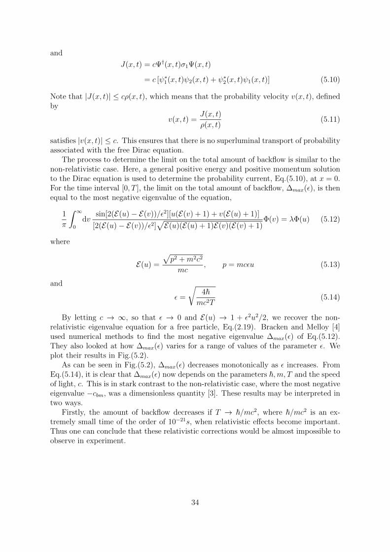
The process to determine the limit on the total amount of backflow is similar to thenon-relativistic case. Here, a general positive energy and positive momentum solutionto the Dirac equation is used to determine the probability current, Eq.(5.10), at x = 0.For the time interval [0, T ], the limit on the total amount of backflow, ∆max(ε), is thenequal to the most negative eigenvalue of the equation,

1

π

∫ ∞0

dvsin[2(E(u)− E(v))/ε2][u(E(v) + 1) + v(E(u) + 1)]

[2(E(u)− E(v))/ε2]√E(u)(E(u) + 1)E(v)(E(v) + 1)

Φ(v) = λΦ(u) (5.12)

where

E(u) =

√p2 +m2c2

mc, p = mcεu (5.13)

and

ε =

√4~

mc2T(5.14)

By letting c → ∞, so that ε → 0 and E(u) → 1 + ε2u2/2, we recover the non-relativistic eigenvalue equation for a free particle, Eq.(2.19). Bracken and Melloy [4]used numerical methods to find the most negative eigenvalue ∆max(ε) of Eq.(5.12).They also looked at how ∆max(ε) varies for a range of values of the parameter ε. Weplot their results in Fig.(5.2).

As can be seen in Fig.(5.2), ∆max(ε) decreases monotonically as ε increases. FromEq.(5.14), it is clear that ∆max(ε) now depends on the parameters ~,m, T and the speedof light, c. This is in stark contrast to the non-relativistic case, where the most negativeeigenvalue −cbm, was a dimensionless quantity [3]. These results may be interpreted intwo ways.

Firstly, the amount of backflow decreases if T → ~/mc2, where ~/mc2 is an ex-tremely small time of the order of 10−21s, when relativistic effects become important.Thus one can conclude that these relativistic corrections would be almost impossible toobserve in experiment.

34

0.2 0.4 0.6 0.8 1.0Ε

-0.038

-0.036

-0.034

-0.032

-0.030

-0.028

-0.026

DmaxHΕL

Figure 5.2: Plot of the most negative eigenvalue of Eq.(5.12), ∆max(ε) as a function ofε.

Alternatively, if we choose to fix c, then the most negative value of ∆max(ε) emergesif T →∞, m→∞ or ~→ 0. In the naive classical limit ~→ 0, the amount of probabil-ity backflow increases. Although this “limit” is an oversimplification, one would expectthis clearly non-classical effect to vanish. It is worrying that this is so, however it doescoincide with the non-relativistic case, where taking ~→ 0 does not cause backflow todisappear.

5.4 Backflow Against a Constant Force

If a non-relativistic particle is subject to a constant force F > 0 in the positivex-direction, how much probability backflow can occur in opposition to this force over agiven time interval [0, T ]? This question was posed by Bracken and Melloy [6]. Similarto the case of a free particle [3], and Dirac electron [4], the problem becomes one ofsolving an eigenvalue equation of the form,

1

π

∫ ∞0

dvsin[u2 − v2 + α(u− v)]

(u− v)φ(v) = λφ(u) (5.15)

where α is a dimensionless parameter defined by

α =FT

32

√4m~

(5.16)

Note that if F = 0 then α = 0 and we recover the non-relativistic eigenvalue equationfor a free particle, Eq.(2.19). Using numerical methods, the most negative eigenvalue∆max(α) of Eq.(5.15) was calculated for a chosen set of values of α. The results are

35

displayed in Fig.(5.3), and reveal the relationship,

∆max(α) = −0.039e−2α (5.17)

0.2 0.4 0.6 0.8 1.0 1.2 1.4Α

-0.035

-0.030

-0.025

-0.020

-0.015

-0.010

-0.005

DmaxHΑL

Figure 5.3: Plot of the most negative eigenvalue of Eq.(5.15), ∆max(α) as a function ofα.

As α increases, the value of ∆max(α) is suppressed by the exponential and decreases.Through Eq.(5.16), it is apparent that ∆max(α) now depends on the parameters F,m, Tand ~. In the limit ~→ 0, the backflow effect decreases as one would hope. This is alsothe case for increasing F or T . What is surprising is that ∆max(α) actually increasesfor increasing m.

5.5 Concluding Remarks

The focus of the material presented in this chapter was to highlight different sit-uations where the most negative eigenvalue −cbm, which also provides a limit on themaximum possible backflow, becomes dependent on certain physical parameters. Mostnotably an emphasis was placed on the reappearance of ~, since letting ~→ 0 is regardedas restoring the classical limit. Backflow was seen to diminish in both the quasiprojec-tor measurement model and in opposition to a constant force when ~ → 0. This wasnot the case for a relativistic particle, however this does agree with the non-relativistictreatment where taking ~ → 0 does not result in the disappearance of the effect. Theprocess of decoherence provides the best explanation as to why backflow is not evidentin classical systems, but by studying these three scenarios a better understanding ofthe effect has been acquired.

36

6 Experimental Realisation

6.1 Introduction

It is of great importance that backflow be observed experimentally. This peculiareffect first noted by Allcock [2], emerged in the context of the arrival time problem inquantum mechanics. It has been argued that the time of arrival of a free particle cannotbe accurately measured [29], and so one might suspect there to be an inherent difficultyin measuring backflow. It is certainly surprising that no one has yet attempted to doso but exactly what method would be most effective is unclear.

The probability current J is used extensively in the literature on backflow but isgenerally regarded as being of no operational significance. Attempts have been madeto relate the current to measurement [30, 31] and it has even been suggested that Jis fundamental in the understanding of scattering phenomena [32]. The most interest-ing treatment examines special protective measurements of J which do not disturb thewave function [33]. The arguments put forward strongly favour associating physicalreality with the quantum state of a single system and these sentiments are reinforcedby recent work [34]. If progress is made in determining the current experimentally,the process would naturally lend itself to a measurement of backflow. In this chapterwe discuss both direct and indirect methods that may lead to the experimental reali-sation of backflow. It is felt that for the subject to advance, the effect must be observed.

6.2 Direct Measurement of Backflow

The most direct method of measuring backflow could in principle be done by makingposition measurements on ensembles of single-particle systems. The flux, Eq.(2.14), canbe defined as

F (t1, t2) = 〈Π(t2)〉 − 〈Π(t1)〉 (6.1)

which is the difference between two probabilities. If we possessed two identical ensem-bles, each prepared in the initial state |ψ〉, then it is possible to deduce the flux. Ameasurement on the first ensemble to determine if the particle is in x > 0 at time t1,would yield 〈Π(t1)〉. The same measurement performed on the second ensemble at timet2, would give 〈Π(t2)〉. If 〈Π(t1)〉 > 〈Π(t2)〉, the flux, Eq.(6.1), is negative and there isbackflow.

Yearsley et al [1] suggest that this could be achieved using a weakly interactingBose-Einstein condensate, since a single measurement on the condensate is effectivelya measurement on an ensemble of non-relativistic particles. The main challenge is thepreparation of identical initial states consisting of only positive momentum. As we sawearlier in Sec.(4.3), a superposition of Gaussian wavepackets is experimentally viablebut does not produce a large amount of backflow. One may ask the question; whatstate can be prepared experimentally to demonstrate backflow? The answer potentially

37

is a Schrodinger cat state, and we will discuss this in Sec.(6.4).Bracken and Melloy [3] propose that a more practicable alternative would be to mea-

sure the electric current density, since this is proportional to the probability current,for an electrically charged particle. The initial states of the particles must be preparedwith only positive velocity components but these can be of arbitrary size. For eachparticle a measurement of the electric current density is made at subsequent intervalsof time. If one were to observe a current density in direct opposition to the velocity(multiplied by the charge), then this would confirm the presence of backflow. Howeverthe feasibility of such a scheme is questionable. One must measure to great accuracy anextremely small amount of current due to a single electric charge moving on the scaleof micrometres per microsecond. The delicate nature of such a measurement, and alsoits reproducibility, suggest it is unlikely that backflow will be observed in this way.

6.3 Complex Potential Model for Arrival Time

The arrival time problem is inextricably linked with the backflow effect. Here, weare concerned with finding the probability that an incoming wavepacket arrives at x = 0during a fixed time interval. There exist many different approaches to this problem [35–39], but in some specific models it is possible to extract the current explicitly from thearrival time probability. For states displaying backflow the current is negative whereasthe arrival time probability is non-negative. A noticeable difference between these twoquantities will give a clear indication of backflow.

We consider an initial wavepacket localised in x < 0 consisting entirely of posi-tive momenta and introduce a complex absorbing potential, −iV0θ(x), of step functionform in x > 0. (See Ref. [9, 40–42] for other arrival time approaches with a complexpotential). The total non-hermitian Hamiltonian is

H = H0 − iV0θ(x) (6.2)

where H0 is the free Hamiltonian. The probability that the wavepacket is in x < 0 andhas yet to be absorbed by the complex potential is given by the survival probabilityN(τ), defined as

N(τ) = 〈ψτ |ψτ 〉 (6.3)

where the state |ψ〉, evolved for a time τ with the complex Hamiltonian Eq.(6.2), isdescribed by

|ψτ 〉 = exp(−iH0 − V0θ(x))τ |ψ〉 (6.4)

The probability for the wavepacket to cross x = 0 in the time interval [τ, τ +dτ ] is thenthe arrival time distribution,

Π(τ) = −dN

dτ

= 2V0〈ψτ |θ(x)|ψτ 〉 (6.5)

If we differentiate with respect to τ then

38

dΠ

dτ= −2V0Π + 2V0〈ψτ |J |ψτ 〉 (6.6)

where J is the current operator, Eq.(2.13). We see that Eq.(6.6) is a differential equationfor Π(τ) and can be solved to give

Π(τ) = 2V0

∫ τ

−∞dt e−2V0(τ−t)〈ψτ |J |ψτ 〉 (6.7)

Assuming Π(τ) → 0 as τ → −∞, then Eq.(6.7) is the exact expression for Π(τ)and shows the explicit dependence on the current operator J . Although J is not apositive operator, Eq.(6.7) is positive by construction. How backflow will affect Π(τ)is unclear, so it is helpful to only consider the usual weak measurement approximationwhere V0 is taken to be small and we may neglect the complex potential term in |ψτ 〉.The arrival time distribution is then

Π(τ) ≈ 2V0

∫ τ

0

dt e−2V0(τ−t)〈ψt|J |ψt〉

= 2V0

∫ τ

0

dt e−2V0(τ−t)J(t) (6.8)

where |ψt〉 = e−iH0t|ψ〉. The distribution Π(τ) is no longer strictly positive because thecurrent may be negative for states that display backflow. Even integration over timedoes not necessarily ensure the positivity of Eq.(6.8). We only took the limit V0 → 0for the complex potential term in |ψτ 〉, but not in the rest of the expression, so thepositivity observed in Eq.(6.7) is not preserved. However, for sufficiently small V0 thisis not significant, and Π(τ) can be regarded as the arrival time distribution measuredby a realistic measurement. This in principle can be determined experimentally andby using the process of deconvolution [43, 44], the current (and consequently the flux),can be calculated from Eq.(6.8).

For states that exhibit backflow the flux is negative, whereas the probability forcrossing x = 0 during the time interval [t1, t2], defined as

P(t1, t2) =

∫ t2

t1

dtΠ(t) (6.9)

is a strictly positive quantity. A comparison of the two values provides a way to poten-tially observe backflow if there is a significant difference between them.

Note that Eq.(6.8) has the form of the current smeared over a period of time. Aregion of negative current will counteract and essentially cancel out a region of positivecurrent in the measured probability Π(τ). It is possible then, that backflow causesa time delay between the arrival of the wavepacket at x = 0 and its detection in ameasuring device.

Already it has been shown that for an idealised particle detection model that uses acomplex potential, the backflow effect has startling implications when considering theconcept of perfect absorption at the origin [10]. During an interval of backflow it is

39

possible for a perfect absorber to emit probability. This is to compensate for the smallamount of probability that has already entered the detector volume before the periodof backflow, but has not been absorbed. The effect is only temporary however and noparticles are permanently reflected if we are to assume the detector behaves as a perfectabsorber. We also mention that at asymptotic distances from the source or interactionregion, the effect of backflow is negligible [9].

Yearsley et al [1] looked at how probability backflow is affected by a time-smearedcurrent. Their plot of the current for the backflow maximising state, compared withthe time-smeared current Eq.(6.8) for two values of V0, can be seen in Fig.(6.1).

Figure 6.1: A comparison of the backflow maximising current (solid line) with thetime-smeared current Eq.(6.8) for V0 = 0.5 (dashed line) and V0 = 0.1 (dotted line) [1].

There are no longer any periods of negativity due to the time-smearing of the cur-rent. The behaviour at t = ±1 is now characterized by discontinuous changes in thederivative of the time-smeared current rather than the distinctive singularity structure.These discontinuities are possible signatures (in the measured probabilities) of the back-flow effect.

6.4 Schrodinger Cat State

A Schrodinger cat state is a superposition of two maximally different quantum states.For our purposes we are interested in a superposition of spatially separated coherentstates described by the wave function,

|ψcat〉 = a|α〉+ b| − α〉 a, b ∈ C (6.10)

where |α〉 is a coherent state which is specified by a single complex number α. Coher-

40

ent states are minimum uncertainty states, and in the position representation can beexpressed as

ψα(x) = 〈x|α〉 = A exp

(−(√

mω

2~x+ α

)2)

(6.11)

where A is a normalisation constant given by,

A =(mωπ~

) 14

exp

(1

2α(α− α∗)

)(6.12)

The time dependence of the coherent state is obtained by acting with the time evolutionoperator U(t) = exp(−iHt/~), and it follows that

U(t)|α〉 = |α(t)〉 = e−i2ωt|αe−iωt〉 (6.13)

A coherent state remains coherent as time evolves. The time dependent wave functionof the cat state, expressed in the position representation, is now

ψcat(x, t) = aψα(x, t) + bψ−α(x, t) (6.14)

The state ψcat(x, t) is a superposition with arbitrary weights of two coherent statessymmetrically placed with respect to the origin. The preparation of cat states is chal-lenging as they are very susceptible to decoherence, but states of this form have beenrealised experimentally [45, 46]. Most notably, a cat state of the harmonic oscillator hasbeen created by preparing a superposition of two coherent state wavepackets of a singletrapped ion in one dimension [47, 48]. This approach enables the harmonic motion ofthe trapped ion to be controlled to a high degree of accuracy, and because of the timeevolution of a coherent state, the separation of the superposition is preserved.

It is the motion of the ion in the trap that may lead to the observation of backflow.For the effect to occur, one of the two components of the wave function must overtakeand interfere with the other. However, ψcat(x, t) is a symmetric state and will not dis-play backflow. It is experimentally possible though, to manipulate ψcat(x, t) so that itis no longer symmetric. This is achieved by applying a single pulse of an additional dcelectric field to displace the ion from the trap centre. The cat state will then be of theform,

|ψcat〉 = a|α〉+ b|β〉 (6.15)

where α and β are real and non-negative, and this state will produce backflow. A plotof the current Eq.(2.2), at x = 0, is shown in Fig.(6.2) and Fig.(6.3) for the followingparameters,

a =

√3

4, b =

√1

4, α = 1.5, β = 9, ω = 1 (6.16)

with ~ = 1 and m = 1. The parameters chosen were to illustrate the negativity of thecurrent and in principle are experimentally viable.

41

0.5 1.0 1.5 2.0 2.5 3.0t

-1

1

2

3

4

5

JH0, tL

Figure 6.2: Plot of J(0, t) for a wave function consisting of a superposition of twocoherent states, with the parameters specified in Eq.(6.16).

1.4 1.5 1.6 1.7 1.8t

-0.5

0.5

JH0, tL

Figure 6.3: Close up of Fig.(6.2). The current is clearly seen to be negative at severaltimes.

The current has two strong negative peaks for the time interval [0, π], best seenin Fig.(6.3). A plot of the probability for remaining in x < 0 is shown in Fig.(6.4).Like the example of a superposition of two Gaussian wavepackets in Sec.(4.3), backflowoccurs in several disjoint time intervals. The value of the flux during the largest periodof backflow is calculated to be,

F ≈ −0.0116 (6.17)

42

which is around 30% of the theoretical maximum. The backflowing fraction of thex-axis has the value,

Pback = 0.1404 (6.18)

Both the negative flux and Pback are larger for the cat state when compared with asuperposition of two Gaussians. This is encouraging for the experimental observationof the effect, even though the amount of backflow is still significantly less than thetheoretical maximum.

0.5 1.0 1.5 2.0 2.5 3.0t

0.2

0.4

0.6

0.8

1.0

PHtL

Figure 6.4: Plot of the probability for remaining in x < 0 as a function of time for theSchrodinger cat state.

1.5 1.6 1.7 1.8t

0.3

0.4

0.5

0.6

0.7

0.8

PHtL

Figure 6.5: Close up of Fig.(6.4). The probability is clearly seen to increase.

43

It is possible to increase the amount of backflow by modifying the values of α and β.However, a Schrodinger cat state has support on both positive and negative momentumtherefore it is necessary to confirm the occurrence of backflow is not the result of anynegative momenta in the wavepacket. A series of plots of the momentum distributionof the cat state for various times during the interval, 0 ≤ t ≤ π, is shown in Fig.(6.6).At t = 0.8, the cat state is almost entirely composed of positive momentum. Duringa period of backflow (t = 1.6), the momentum distribution of |α〉 is centred aroundp ≈ 2.1, and an estimate of the fraction of the wavepacket located in p < 0 shows ap-proximately 0.1% of the wavepacket consists of negative momentum. This is negligibleand demonstrates that the negativity of the flux is due to the backflow effect.

Note that the Wigner function of a cat state displays Gaussian like probabilitieslocalised in two different regions of phase space plus a strong interference term whichtakes negative values [49]. As discussed in Sec.(2.1), it is this negativity that is a nec-essary condition for the negativity of the flux.

Figure 6.6: Plot of the momentum distribution of the Schrodinger cat state for varioustimes during the interval, 0 ≤ t ≤ π.

A method similar to that described in Sec.(6.2) could be used to detect backflow.Position measurements on the ion must be performed with a temporal resolution thatis less than the period of the trap. Shining a laser on the ion at resonance will emit alarge number of photons that would indicate its position, however there are concernswith this approach. A laser can impart more momentum to the ion which may disturb

44

the harmonic motion and more importantly, any measurement that reveals the positionof the ion to within the uncertainty of its wave function will destroy the quantumstate. An indirect method could prove more fruitful, but precisely what this mightentail is unclear. It is important that any interaction with the state does not lead todecoherence. The field of ion trap manipulation is now well established and one suspectsthat the techniques required to detect backflow already exist. All that is needed is anexperimentalist with the expertise to finally realise this quantum effect.

The material presented in this section is in its infancy but does show promise.Further work must establish the optimum values for α and β to maximise backflow butalso confirm that negative momentum is not responsible. It could be that experimentallimitations mean only a small range of values are accessible to α and β.

45

7 Summary and Further Work

7.1 Summary

The aim of this report was to provide a detailed account of the quantum backfloweffect. In Chapter 2 it was shown that when the current at the origin J(0, t) < 0, theprobability of remaining in x < 0 can increase with time. To understand this behaviourwe developed the relationship between the Wigner function and the current. Negativevalues of the Wigner function arise from interference between different portions of thewavepacket and it is this negativity that is a necessary condition for the negativity ofthe current. The backflow eigenvalue equation was set up and solved numerically tofind the most negative eigenvalue of the flux operator. This led to the appearance of thedimensionless quantity cbm. The backflow maximising state was numerically computedand a plot of the resulting wave function shown in momentum and configuration space.A plot of the resulting current revealed a distinctive singularity structure at t = ±1.The flux operator was shown to be linear bounded, self-adjoint and non-compact.

The spatial extent of backflow was explored in Chapter 3. A quantum inequality forthe current demonstrated that backflow is limited in space. The backflowing fractionof the x-axis was characterised by the backflow probability Pback, which approaches itsmaximal value of 1/2 when the component momenta in the wavepacket are stronglycorrelated. The connection between backflow and superoscillations was explored. Thereappeared to be striking similarities between the time evolution of fast superoscillationsand strong backflow.

In Chapter 4 the example of a superposition of two plane waves was used to illus-trate the backflow effect. This demonstrated that negative values of the current can beunderstood as an interference effect. It was also shown that the width of a region ofbackflow decreases as the wavenumber k(x) becomes more negative. The current andthe flux were computed for a superposition of two Gaussian wavepackets. Althoughexperimentally realisable, this state displays only 16% of the maximum possible back-flow, a very small amount. A normalisable state significant in the development of thesubject was studied and shown to display 11% of the theoretical maximum backflow.A candidate analytic expression for the backflow maximising state was presented whichappeared to follow closely the numerical solution of Penz et al [8]. However a plot of thecurrent failed to match the distinctive singularity structure at t = ±1 which is perhapsan important characteristic of the backflow maximising state.

In Chapter 5 we examined three different scenarios where the most negative eigen-value −cbm, becomes dependent on certain physical parameters. The more realisticmeasurement model of quasiprojectors restored the naive classical limit, and backflowwas seen to diminish when ~→ 0. In the relativistic case for particles governed by theDirac equation, the maximum amount of backflow ∆max depends on the dimensionlesscombination mc2T/~. Backflow can occur in opposition to a constant force but theeffect gets smaller when the size of the force is increased.

46

The experimental realisation of backflow was discussed in Chapter 6. A directmethod to measure backflow could in principle be done by making position measure-ments on ensembles of single-particle systems. A complex potential model often used inthe arrival time problem could lead to the observation of backflow. If the arrival timedistribution Π(τ) can be determined, it is possible to extract the current by deconvo-lution and then from this calculate the flux. Backflow was also noted to have certainimplications for the concept of perfect absorption. A Schrodinger cat state which isexperimentally realisable was shown to exhibit backflow. The scheme presented showspromise but requires further work.

7.2 Open Questions and Further Work

Time Scale of Backflow

It is always possible to find a state which exhibits backflow for an arbitrarily long periodof time but this does not tell us about the ‘natural’ time scale for which this effecttakes place. The relationship established in Eq.(2.24) demonstrated that the currentcan be arbitrarily negative if only for a sufficiently short time. Does the magnitude ofthe negative current dictate the time scale on which backflow occurs? If not, is it someproperty of the type of state that determines the duration of a period of backflow? Thesequestions reaffirm the need for experimental observation of the effect. If a successfulmethod to determine the flux was found, the amount of backflow for different statescould be measured and compared not only with each other, but also their own theoreticalmaximum values. This would establish whether or not a state will always display thesame amount of backflow.

Analytic Calculation of the Eigenvalue Equation

Penz et al [8] questioned whether there really is a backflow eigenvalue, in the strictmathematical sense, that −cbm is an approximation to. The analytic calculation of−cbm and the analytic form of the backflow maximising state will no doubt be foundif there is a continued effort to do so. This optimism is confirmed by the progressmade in the recent work of Yearsley et al [1], who also speculate that perhaps the non-commutativity of the operators θ(p) and θ(−x) will lead to an analytic calculation ofthe quantity −cbm.

Eigenstates of the Flux Operator

The backflow maximising state is an eigenstate of the flux operator F (t1, t2) with eigen-value −cbm. Here is a quantum state that describes a non-relativistic free particle whichdisplays the maximum amount of backflow. How does one interpret the other eigenstatesof the flux operator though? Specifically what does it mean for the eigenstate whichhas eigenvalue +1? A plot of this state in momentum space is shown in Fig.(7.1). It hasa slightly different form to the backflow maximising state Fig.(2.1). The behaviour atlarge u is unclear because a momentum cut-off must be introduced to solve the backfloweigenvalue equation numerically. It would appear that the state tends towards someasymptotic form, however further investigation is needed.

47

5 10 15 20u

-0.04

-0.02

0.00

0.02

0.04

ΦHuL

Figure 7.1: Plot of the eigenstate of the flux operator with eigenvalue +1 in momentumspace.

A plot of the current at the origin is shown in Fig.(7.2). There are large positivevalues of J , but also short periods of negativity indicating that this eigenstate exhibitsbackflow too. Since the flux of this state is +1, the probability for remaining in x < 0rapidly decreases with all the probability crossing x = 0 in the time interval [−1, 1].This suggests the eigenstate consists of a wavepacket with high velocity which crossesthe origin in its entirety during [−1, 1].

-1.0 -0.5 0.5 1.0t

-2

2

4

6

8

jHtL

Figure 7.2: Plot of J(0, t) for the eigenstate of the flux operator with eigenvalue +1.

It would be of great interest to look in more detail at the other eigenstates of theflux operator. Not only would it help our interpretation of these states but it could wellprovide clues to the analytic form of the backflow maximising state.

48

References

[1] J.M.Yearsley, J.J.Halliwell, R.Hartshorn, and A.Whitby,e-print arXiv:1202.1783v4 (2012).

[2] G.R.Allcock, Ann.Phys. 53, 253 (1969); 53, 286 (1969); 53, 311 (1969).

[3] A.J.Bracken and G.F.Melloy, J.Phys.A 27, 2197 (1994).

[4] A.J.Bracken and G.F.Melloy, Found.Phys. 28, 505 (1998).

[5] M.V.Berry, J.Phys.A 43, 415302 (2010).

[6] A.J.Bracken and G.F.Melloy, Ann.Phys.(Leipzig) 7, 726 (1998).

[7] S.P.Eveson, C.J.Fewster, and R.Verch, Ann.Inst. H.Poincare 6, 1 (2005).

[8] M.Penz, G.Grubl, S.Kreidl, and P.Wagner, J.Phys.A 39, 423 (2006).

[9] J.G.Muga, S.Brouard, and D.Macıas, Ann.Phys. 240, 351 (1995).

[10] J.G.Muga, J.P.Palao, and C.R.Leavens, Phys.Lett.A 253, 21 (1999).

[11] M.Ruggenthaler, G.Grubl, and S.Kreidl, J.Phys.A 38, 8445 (2005).

[12] P.Strange, Eur.J.Phys. 33, 1147 (2012).

[13] J.M.Yearsley, Phys.Rev.A 82, 012116 (2010).

[14] J.J.Halliwell and J.M.Yearsley, Phys.Rev.A 79, 062101 (2009).

[15] J.M.Yearsley, Aspects of Time in Quantum Theory, Imperial College PhD Thesisavailable as quant-ph/1110.5790 (2011).

[16] J.J.Halliwell and J.M.Yearsley, Phys.Lett.A 374, 154 (2009).

[17] B.Misra and E.C.G.Sudarshan, J.Math.Phys. 18, 756 (1977).

[18] N.Balasz and B.K.Jennings, Phys.Rep. 104, 347 (1984).M.Hillery, R.F.O’Connell, M.O.Scully, and E.P.Wigner, Phys.Rep. 106, 121(1984).

[19] R.P.Feynman, Quantum Implications: Essays in Honour of David Bohm, B.J.Hileyand F.D.Peat (eds) p. 235 (Routledge and Kegan Paul, 1987).

[20] L.Diosi and C.Kiefer, J.Phys.A 35, 2675 (2002).P.J.Dodd and J.J.Halliwell, Phys.Rev.A 69, 052105 (2004).

[21] N.N.Bogolubov, A.A.Logunov, A.I.Oksak, and I.T.Todorov, General Principles ofQuantum Field Theory p. 100 (Kluwer Academic Publishers, Dordrecht, 1990).

49

[22] Y.Aharonov, J.Anadan, S.Popescu, and L.Vaidman, Phys.Rev.Lett. 64, 2965(1990).

[23] Y.Aharonov, D.Z.Albert, and L.Vaidman, Phys.Rev.Lett 60, 1351 (1988).

[24] M.V.Berry and P.Shukla, J.Phys.A 43, 354024 (2010).

[25] Y.Aharonov, F.Colombo, I.Sabadini, D.C.Struppa, and J.Tollaksen, J.Phys.A 44,365304 (2011).

[26] M.V.Berry and S.Popescu, J.Phys.A 39, 6965 (2006).

[27] J.H.Eberly, N.B.Narozhny, and J.J.Sanchez-Mondragon, Phys.Rev.Lett. 44, 1323(1980).

[28] P.J.S.G.Ferreira and A.Kempf, IEEE Trans.Signal Processing 54, 3732 (2006).

[29] Y.Aharonov, J.Oppenheim, S.Popescu, B.Reznik, and W.G.Unruh, Phys.Rev.A57, 4130 (1998).

[30] W.Gale, E.Guth, and G.T.Trammell, Phys.Rev. 165, 1434 (1968).

[31] D.J.Mason, M.F.Borunda, and E.J.Heller, cond-mat/1205.0291 (2012).

[32] M.Daumer, D.Durr, S.Goldstein, and N.Zanghi, J.Stat.Phys. 88, 967 (1997).

[33] Y.Aharonov and L.Vaidman, Phys.Lett.A 178, 38 (1993).

[34] M.F.Pusey, J.Barrett, and T.Rudolph, Nature Physics 8, 476 (2012).

[35] N.Grot, C.Rovelli, and R.S.Tate, Phys.Rev.A 54, 4676 (1996).

[36] V.Delgado and J.G.Muga, Phys.Rev.A 56, 3425 (1997).

[37] J.G.Muga and C.R.Leavens, Phys.Rep. 338, 353 (2000).

[38] J.G.Muga, R.Sala Mayato, and I.L.Egusquiza (eds), Time In Quantum Mechanics(Springer, Berlin, 2002).

[39] J.M.Yearsley, D.A.Downs, J.J.Halliwell, and A.K.Hashagen, Phys.Rev.A 84,022109 (2011).

[40] J.J.Halliwell, Prog.Th.Phys. 102, 707 (1999).

[41] J.Echanobe, A.del Campo, and J.G.Muga, Phys.Rev.A 77, 032112 (2008).

[42] J.J.Halliwell, Phys.Rev.A 77, 062103 (2008).

[43] J.A.Damborenea, I.L.Egusquiza, G.C.Hegerfeld, and J.G.Muga, Phys.Rev.A 66,052104 (2002).

[44] G.C.Hegerfeld, D.Seidel, and J.G.Muga, Phys.Rev.A 68, 022111 (2003).

[45] D.Leibfried et al, Nature 438, 639 (2005).

50

[46] X.C.Yao et al, Nature Photon. 6, 225 (2012).

[47] C.Monroe, D.M.Meekhof, B.E.King, and D.J.Wineland, Science 272, 1131 (1996).

[48] C.Monroe, D.M.Meekhof, B.E.King, D.Liebfried, W.M.Itano, and D.J.Wineland,Acc.Chem.Res. 29, 585 (1996).

[49] E.Colavita and S.Hacyan, Rev.Mex.Fis. 49, 45 (2003).

51