1

The QC Relaxation: A Theoretical andComputational Study on Optimal Power Flow

Carleton Coffrin, Hassan L. Hijazi, and Pascal Van Hentenryck

Abstract—Convex relaxations of the power flow equations and,in particular, the Semi-Definite Programming (SDP) and Second-Order Cone (SOC) relaxations, have attracted significant interestin recent years. The Quadratic Convex (QC) relaxation is a depar-ture from these relaxations in the sense that it imposes constraintsto preserve stronger links between the voltage variables throughconvex envelopes of the polar representation. This paper is asystematic study of the QC relaxation for AC Optimal PowerFlow with realistic side constraints. The main theoretical resultshows that the QC relaxation is stronger than the SOC relaxationand neither dominates nor is dominated by the SDP relaxation.In addition, comprehensive computational results show thatthe QC relaxation may produce significant improvements inaccuracy over the SOC relaxation at a reasonable computationalcost, especially for networks with tight bounds on phase angledifferences. The QC and SOC relaxations are also shown to besignificantly faster and reliable compared to the SDP relaxationgiven the current state of the respective solvers.

Index Terms—Optimization Methods, Convex Quadratic Op-timization, Optimal Power Flow

NOMENCLATURE

N - The set of nodes in the networkE - The set of from edges in the networkER - The set of to edges in the networki - imaginary number constantI - AC currentS “ p` iq - AC powerV “ v=θ - AC voltageZ “ r ` ix - Line impedanceY “ g ` ib - Line admittanceT “ t=θt - Transformer propertiesY s “ gs ` ibs - Bus shunt admittanceW - Product of two AC voltagesl - Current magnitude squared, |I|2

bc - Line chargingsu - Line apparent power thermal limitθ∆ - Phase angle difference limitSd “ pd ` iqd - AC power demandSg “ pg ` iqg - AC power generationc0, c1, c2 - Generation cost coefficients<p¨q - Real part of a complex number=p¨q - Imaginary part of a complex numberp¨q˚ - Conjugate of a complex number| ¨ | - Magnitude of a complex number, l2-normxl, xu - Lower and upper bounds of x, respectivelyqx - Convex envelope of xx - A constant value

All authors are members of the Optimisation Research Group, NICTA, ACT2601 Australia; and affiliated with the College of Engineering and ComputerScience, Australian National University, ACT 0200, Australia.

I. INTRODUCTION

CONVEX relaxations of the power flow equations haveattracted significant interest in recent years. They in-

clude the Semi-Definite Programming (SDP) [1], Second-Order Cone (SOC) [2], Convex-DistFlow (CDF) [3], and therecent Quadratic Convex (QC) [4] and Moment-Based [5],[6] relaxations. Much of the excitement underlying this lineof research comes from the fact that the SDP relaxation hasshown to be tight on a variety of case studies [7], openinga new avenue for accurate, reliable, and efficient solutionsto a variety of power system applications. Indeed, industrial-strength optimization tools (e.g., Gurobi, cplex, Mosek) arenow available to solve various classes of convex optimizationproblems.

The relationships between the SDP, SOC, and CDF re-laxations is now largely well-understood: See [8], [9] for acomprehensive overview. In particular, the SOC and CDFrelaxations are known to be equivalent and the SDP relaxationis at least as strong than both of these. However, little isknown about the QC relaxation which is a significant departurefrom these more traditional relaxations. Indeed, one of the keyfeatures of the QC relaxation is to compute convex envelopesof the polar representation of the power flow equations inthe hope of preserving stronger links between the voltagevariables. This contrasts with the SDP and SOC relaxationswhich are derived from a lift-and-project approach on thecomplex representation.

This paper fills this gap and provides a theoretical study ofthe QC relaxation as well as a comprehensive computationalevaluation to compare the strengths and weaknesses of theserelaxations. Our main contributions can be summarized asfollows:

1) The QC relaxation is stronger than the SOC relaxation.2) The QC relaxation neither dominates nor is dominated

by the SDP relaxation.3) Computational results on optimal power flow show that

the QC relaxation may bring significant benefits inaccuracy over the SOC relaxation, especially for tightbounds on phase angle differences, for a reasonable lossin efficiency.

4) The computational results also show that, with existingsolvers, the SOC and QC relaxations are significantlyfaster and more reliable than the SDP relaxation.

The theoretical results are derived using the equivalence of twoclasses of second-order cone constraints (in conjunction withthe power equations), which provides an alternative formula-tion for the QC model which is interesting in its own right.

arX

iv:1

502.

0784

7v2

[cs

.CE

] 2

9 Ju

l 201

5

2

Moreover, to the best of our knowledge, the computationalresults also represent the most comprehensive comparison ofthese convex relaxations. They are obtained for optimal powerflow problems with realistic side-constraints, featuring busshunts, line charging, and transformers.

The rest of the paper is organized as follows. Section IIreviews the formulation of the AC-OPF problem from firstprinciples and presents two equivalent formulations of thisnon-convex optimization problem. Section III derives the SDP,QC, and SOC relaxations. Section IV illustrates their behavioron a well-known 3-bus example. Section V presents an alter-native formulation of the QC relaxation which is a convenienttool for subsequent proofs. Section VI presents the theoreticalresults linking the QC to the other relaxations. Section VIIreports the computational results for the three relaxations on93 AC-OPF test cases, and Section VIII concludes the paper.

II. AC OPTIMAL POWER FLOW

This section reviews the specification of AC Optimal PowerFlow (AC-OPF) and introduces the notations used in the paper.In the equations, constants are always in bold face. The ACpower flow equations are based on complex quantities forcurrent I , voltage V , admittance Y , and power S, which arelinked by the physical properties of Kirchhoff’s Current Law(KCL), i.e.,

Igi ´ Idi “

ÿ

pi,jqPEYER

Iij (1)

Ohm’s Law, i.e.,

Iij “ YijpVi ´ Vjq (2)

and the definition of AC power, i.e.,

Sij “ ViI˚ij (3)

Combining these three properties yields the AC Power Flowequations, i.e.,

Sgi ´ Sdi “

ÿ

pi,jqPEYER

Sij @i P N (4a)

Sij “ Y˚ij ViV

˚i ´ Y

˚ij ViV

˚j pi, jq P E Y ER (4b)

These non-convex nonlinear equations define how power flowsin the network and are a core building block in many powersystem applications. However, practical applications typicallyinclude various operational side constraints on the power flow.We now review some of the most significant ones.

Generator Capabilities: AC generators have limitationson the amount of active and reactive power they can produceSg , which is characterized by a generation capability curve[10]. Such curves typically define nonlinear convex regionswhich are typically approximated by boxes in AC transmissionsystem test cases, i.e.,

Sgli ď Sgi ď S

gui @i P N (5a)

Line Thermal Limit: AC power lines have thermal limits[10] to prevent lines from sagging and automatic protectiondevices from activating. These limits are typically given inVolt Amp units and constrain the apparent power flows on thelines, i.e.,

|Sij | ď suij @pi, jq P E Y E

R (6)

Bus Voltage Limits: Voltages in AC power systems shouldnot vary too far (typically ˘10%) from some nominal basevalue [10]. This is accomplished by putting bounds on thevoltage magnitudes, i.e.,

vli ď |Vi| ď vui @i P N (7)

A variety of power flow formulations only have variablesfor the square of the voltage magnitude, i.e., |Vi|2. In suchcases, the voltage bound constrains can be incorporated viathe following constraints:

pvliq2 ď |Vi|

2 ď pvui q2 @i P N (8)

Phase Angle Differences: Small phase angle differencesare also a design imperative in AC power systems [10] and ithas been suggested that phase angle differences are typicallyless than 10 degrees in practice [11]. These constraints havenot typically been incorporated in AC transmission test cases[12]. However, recent work [13], [4] have observed thatincorporating Phase Angle Difference (PAD) constraints, i.e.,

´ θ∆ij ď =`

ViV˚j

˘

ď θ∆ij @pi, jq P E (9)

is useful in the convexification of the AC power flow equa-tions. For simplicity, this paper assumes that the phase an-gle difference bounds are symmetrical and within the rangep´π{2, π{2q, i.e.,

0 ď θ∆ij ďπ

2pi, jq P E (10)

but the results presented here can be extended to more generalcases. Observe also that the PAD constraints (9) can beimplemented as a linear relation of the real and imaginarycomponents of ViV ˚j [14], i.e. @pi, jq P E,

tanp´θ∆ij q<`

ViV˚j

˘

ď=`

ViV˚j

˘

ďtanpθ∆ij q<`

ViV˚j

˘

(11)

The usefulness of this formulation will be apparent later in thepaper.

Other Constraints: Other line flow constraints have beenproposed, such as, active power limits and voltage differencelimits [7], [14]. However, we do not consider them here since,to the best of our knowledge, test cases incorporating theseconstraints are not readily available.

Objective Functions: The last component in formulatingOPF problems is an objective function. The two classicobjective functions are line loss minimization, i.e.,

minimize:ÿ

iPN

<pSgi q (12)

and generator fuel cost minimization, i.e.,

minimize:ÿ

iPN

c2ip<pSgi qq2 ` c1i<pSgi q ` c0i (13)

Observe that objective (12) is a special case of objective (13)where c2i“0, c1i“1, c0i“0 piPNq [15]. Hence, the rest ofthis paper focuses on objective (13).

3

Model 1 AC-OPF

variables: Sgi p@i P Nq, Vip@i P Nq

minimize:ÿ

iPN

c2ip<pSgi qq2 ` c1i<pSgi q ` c0i (15a)

subject to:

vli ď |Vi| ď vui @i P N (15b)

Sgli ď Sgi ď S

gui @i P N (15c)

|Sij | ď suij @pi, jq P E Y E

R (15d)

Sgi ´ Sdi “

ÿ

pi,jqPEYER

Sij @i P N (15e)

Sij “ Y˚ij ViV

˚i ´ Y

˚ij ViV

˚j pi, jq P E Y ER (15f)

´ θ∆ij ď =pViV˚j q ď θ

∆ij @pi, jq P E (15g)

Model 2 AC-OPF-W

variables: Sgi p@i P Nq, Vip@i P Nq, Wijp@i, j P Nq

minimize:ÿ

iPN

c2ip<pSgi qq2 ` c1i<pSgi q ` c0i (16a)

subject to:

Wij “ ViV˚j @i P N,@j P N (16b)

pvliq2 ďWii ď pv

ui q

2 @i P N (16c)

Sgli ď Sgi ď S

gui @i P N (16d)

Sgi ´ Sdi “

ÿ

pi,jqPEYER

Sij @i P N (16e)

Sij “ Y˚ijWii ´ Y

˚ijWij pi, jq P E (16f)

Sji “ Y˚ijWjj ´ Y

˚ijW

˚ij pi, jq P E (16g)

|Sij | ď psuijq @pi, jq P E Y E

R (16h)

tanp´θ∆ij q<pWijq ď =pWijq ď tanpθ∆ij q<pWijq (16i)

@pi, jq P E

AC-OPF: Combining the AC power flow equations, theside constraints, and the objective function, yields the well-known AC-OPF formulation presented in Model 1. Observethat, in Model 1, the non-convexities arises solely from theproduct of the voltages (i.e., ViV ˚j ) and they can be isolatedby introducing new W variables to represent the products ofV s [16], [2], [17], [18], i.e,

ViV˚j “Wij pi, j P Nq. (14)

Model 2 presents an equivalent version of the AC-OPF, wherethe W factorization has been incorporated and the only sourceof non-convexity is in constraint (16b). Note that this sectionhas introduced the simplest form of the AC-OPF problem andthat real-world applications feature a variety of extensionsas discussed at length in [19], [20]. In practice, this non-convex nonlinear optimization problem is typically solved withnumerical methods (e.g. IPM, SLP) [21], [22], which providelocally optimal solutions if they converge to a feasible point.

Model 3 The SDP Relaxation AC-OPF-W-SDP.

variables: Sgi p@i P Nq, Wijp@i, j P Nq

minimize: (16a)subject to: (16c)–(16i)

W ľ 0 (17a)

Model 4 The SOC Relaxation AC-OPF-W-SOC.

variables: Sgi p@i P Nq, Wijp@pi, jq P Eq, Wiip@i P Nq : real

minimize: (16a)subject to: (16c)–(16i)

|Wij |2 ďWiiWjj @pi, jq P E (18a)

III. CONVEX RELAXATIONS OF OPTIMAL POWER FLOW

Since the AC-OPF problem is NP-Hard [23], [24] andnumerical methods provide limited guarantees for determiningfeasibility and global optimally, significant attention has beendevoted to finding convex relaxations of Model 1. Suchrelaxations are appealing because they are computationallyefficient and may be used to:

1) bound the quality of AC-OPF solutions produced bylocally optimal methods;

2) prove that a particular AC-OPF problem has no solution;3) produce a solution that is feasible in the original non-

convex problem [7], thus solving the AC-OPF andguaranteeing that the solution is globally optimal.

The ability to provide bounds is particularly important for thenumerous mixed-integer nonlinear optimization problems thatarise in power system applications. For these reasons, a varietyof convex relaxations of the AC-OPF have been developed in-cluding, the SDP [1], QC [4], SOC [2], and Convex-DistFlow[3], which are reviewed in detail in this section. Moreover,since the SOC and Convex-DistFlow relaxations have beenshown to be equivalent [25], this paper focuses on the SDP,SOC, and QC relaxations only and shows how they are derivedfrom Model 2. The key insight is that each relaxation presentsa different approach to convexifing constraints (16b), whichare the only source of non-convexity in Model 2.

The Semi-Definite Programming (SDP) Relaxation: ex-ploits the fact that the W variables are defined by V pV ˚qT ,which ensures that W is positive semi-definite (denoted byW ľ 0) and has rank 1 [1], [7], [18]. These conditions aresufficient to enforce constraints (16b) [26], i.e.,

Wij “ ViV˚j pi, j P Nq ô W ľ 0 ^ rankpW q “ 1

The SDP relaxation [27], [26] then drops the rank constraintto obtain Model 3.

The Second Order Cone (SOC) Relaxation: convexifieseach constraint of (16b) separately, instead of considering themglobally as in the SDP relaxation. The SOC relaxation takesthe absolute square of each constraint, refactors it, and then

4

relaxes the equality into an inequality, i.e.,

Wij “ ViV˚j (19a)

WijW˚ij “ ViV

˚j V

˚i Vj (19b)

|Wij |2 “WiiWjj (19c)

|Wij |2 ďWiiWjj (19d)

Equation (19d) is a rotated second-order cone constraint whichis widely supported by industrial optimization tools. It can, infact, be rewritten in the standard form of a second-order coneconstraint as,

ˇ

ˇ

ˇ

ˇ

ˆ

2Wij

Wii ´Wjj

˙ˇ

ˇ

ˇ

ˇ

ďWii `Wjj (20)

The complete SOC formulation is presented in Model 4. Notethat this relaxation requires fewer W variables than Model 3.Due to the sparsity of AC power networks, this size reductioncan lead to significant memory and computational savings.

The Quadratic Convex (QC) Relaxation: was introducedto preserve stronger links between the voltage variables [4].It represents the voltages in polar form (i.e., V “ v=θ) andlinks these real variables to the W variables, along the linesof [16], [17], [28], [29], using the following equations:

Wii “ v2i i P N (21a)

<pWijq “ vivj cospθi ´ θjq @pi, jq P E (21b)=pWijq “ vivj sinpθi ´ θjq @pi, jq P E (21c)

The QC relaxation then relaxes these equations by takingtight convex envelopes of their nonlinear terms, exploiting theoperational limits for vi, vj , θi´ θj . The convex envelopes forthe square and product of variables are well-known [30], i.e.,

xx2yT ”

#

qx ě x2

qx ď pxu ` xlqx´ xuxl(T-CONV)

xxyyM ”

$

’

’

’

&

’

’

’

%

|xy ě xly ` ylx´ xlyl

|xy ě xuy ` yux´ xuyu

|xy ď xly ` yux´ xlyu

|xy ď xuy ` ylx´ xuyl

(M-CONV)

Under our assumptions that the phase angle bound satisfies0 ď θ∆ ď π

2 and is symmetric, convex envelopes for sine(S-CONV) and cosine (C-CONV) [4] are given by,

xsinpxqyS ”

$

&

%

|sx ď cos´

xu

2

¯´

x´ xu

2

¯

` sin´

xu

2

¯

|sx ě cos´

xu

2

¯´

x` xu

2

¯

´ sin´

xu

2

¯

xcospxqyC ”

#

|cx ď 1´ 1´cospxuq

pxuq2x2

|cx ě cospxuq

In the following, we abuse notation and also use xfp¨qyC

to denote the variable on the left-hand side of the convexenvelope C for function fp¨q. When such an expression is usedinside an equation, the constraints xfp¨qyC are also added tothe model.

Convex envelopes for equations (21a)–(21c) can be obtainedby composing the convex envelopes of the functions for

Model 5 The QC Relaxation AC-OPF-C-QC.

variables: Sgi p@i P Nq, Wijp@pi, jq P Eq, Wiip@i P Nq : real

vi=θip@i P Nq, lijp@pi, jq P Eq

minimize: (16a)subject to: (16c)–(16i)

Wii “ xv2i yT i P N (22a)

<pWijq “ xxvivjyM xcospθi ´ θjqy

CyM @pi, jq P E (22b)

=pWijq “ xxvivjyM xsinpθi ´ θjqy

SyM @pi, jq P E (22c)Sij ` Sji “ Zij lij @pi, jq P E (22d)

|Sij |2 ďWiilij @pi, jq P E (22e)

1 2

3

C

Fig. 1. A Network Diagram for the 3-Bus Example.

square, sine, cosine, and the product of two variables, i.e.,

Wii “ xv2i yT i P N (23a)

<pWijq “ xxvivjyM xcospθi ´ θjqy

CyM @pi, jq P E (23b)

=pWijq “ xxvivjyM xsinpθi ´ θjqy

SyM @pi, jq P E (23c)

The QC relaxation also proposes to strengthen these convexenvelopes with a second-order cone constraint based on theabsolute square of line power flow (3), first proposed in [3].This requires a new variable lij for each line pi, jq P Ethat captures the current magnitude squared on that line. Thefollowing constraints are added to link the lij variables to theexisting model variables.

Sij ` Sji “ Zij lij @pi, jq P E (24a)

|Sij |2 ďWiilij @pi, jq P E (24b)

The complete QC relaxation is presented in Model 5. Thismodel is annotated as C-QC, as the second-order cone con-straints use current variables. The motivation for this distinc-tion will become clear in Section V.

IV. AN ILLUSTRATIVE EXAMPLE

This section illustrates the three main power flow relaxationson the 3-bus network from [31], which has proven to be anexcellent test case for power flow relaxations. This system isdepicted in Figure 1 and the associated network parameters aregiven in Table I. This network is designed to have very fewbinding constraints. Hence, the generator and line limits areset to large non-binding values, except for the thermal limitconstraint on the line between buses 2 and 3, which is set to 50MVA. In addition to its base configuration, we also considerthis network with reduced phase angle difference bounds of18˝. IPOPT [32] is used as a heuristic [33] to find a feasible

5

TABLE ITHREE-BUS SYSTEM NETWORK DATA (100 MVA BASE).

Bus ParametersBus pd qd vl vu

1 110 40 0.9 1.12 110 40 0.9 1.13 95 50 0.9 1.1

Line ParametersFrom–To Bus r x bc su θ∆

1–2 0.042 0.90 0.30 8 30˝

2–3 0.025 0.75 0.70 50 30˝

1–3 0.065 0.62 0.45 8 30˝

Generator ParametersGenerator pgl,pgu qgl, qgu c2 c1 c0

1 0,8 ´8,8 0.110 5.0 02 0,8 ´8,8 0.085 1.2 03 0, 0 ´8,8 0 0 0

TABLE IIAC-OPF BOUNDS USING RELAXATIONS ON THE 3-BUS CASE.

$/h Optimality Gap (%)Test Case AC SDP QC SOC

Base 5812 0.39 1.24 1.32θ∆“18˝ 5992 2.06 1.24 4.28

solution to the AC-OPF and we measure the optimally gapbetween the heuristic and a relaxation using the formula

Heuristic´ RelaxationHeuristic

.

Table II summarizes the results.1 In the base configuration, theSDP relaxation has the smallest optimality gap. In the θ∆ “

18˝ case, the QC relaxation has the smallest optimality gap,while reducing the bound on phase angle differences increasesthe optimality gap for both the SDP and SOC relaxations.This small network highlights two important results. First, theSDP relaxation does not dominate the QC relaxation and vice-versa. Second, the SDP and QC relaxations dominate the SOCrelaxation. The next two sections prove that this last resultholds for all networks.

V. AN ALTERNATE FORM OF THE QC RELAXATION

Section III introduced two types of second-order coneconstraints. Model 4 uses a SOC constraint based on theabsolute square of the voltage product [2], i.e.,

|Wij |2 ďWiiWjj (25)

while Model 5 uses a SOC constraint based on the absolutesquare of the power flow [3], i.e.,

|Sij |2 ďWiilij . (26)

We now show that, in conjunction with the power flow equa-tions (16f)–(16g), these two SOC formulations are equivalent.More precisely, we show that

Sij “ Y˚ijWii ´ Y

˚ijWij pi, jq P E

Sji “ Y˚ijWjj ´ Y

˚ijW

˚ij pi, jq P E

|Wij |2 ďWiiWjj pi, jq P E

(W-SOC)

1On this small example a nonlinear global optimization solver was used toprove that the heuristic solutions are in fact globally optimal. Such a validationis not possible on larger test cases.

Model 6 The Alternate QC Relaxation AC-OPF-W-QC

variables: Sgi p@i P Nq, Wijp@pi, jq P Eq, Wiip@i P Nq : real

vi=θip@i P Nq

minimize: (16a)subject to: (16c)–(16i), (22a)–(22c), (18a)

is equivalent to

Sij “ Y˚ijWii ´ Y

˚ijWij pi, jq P E

Sji “ Y˚ijWjj ´ Y

˚ijW

˚ij pi, jq P E

Sij ` Sji “ Zij lij pi, jq P E|Sij |

2 ďWiilij pi, jq P E.

(C-SOC)

This equivalence suggests an alternative formulation of theQC relaxation which is given in Model 6 and establishes aclear connection between Models 4 and 5. Throughout thispaper, we use W and C to denote which of these equivalentformulations is used.

We now prove these results. The following lemma, whoseproof is straight-forward and can be found in the Appendix,establishes some useful equalities.

Lemma V.1. The following four equalities hold:

1) |Sij |2 “ |Yij |2`

W 2ii ´WiiWij ´WiiW

˚ij ` |Wij |

2˘

.2) |Wij |

2 “W 2ii´W

˚iiZ

˚ijSij ´WiiZijS

˚ij ` |Zij |

2|Sij |2.

3) lij “ |Yij |2pWii `Wjj ´Wij ´W

˚ijq.

4) Wjj “Wii ´Z˚ijSij ´ZijS

˚ij ` |Zij |

2lij .

We are now ready to prove the main result of this section.

Theorem V.2. (C-SOC) is equivalent to (W-SOC).

Proof:The proof is similar in spirit to those presented in [25], [34].

W-SOC ñ C-SOC: Every solution to (W-SOC) is asolution to (C-SOC). Given a solution to (W-SOC), by equality(3) in Lemma V.1, we assign lij as follows:

lij “ |Yij |2pWii ´Wij ´W

˚ij `Wjjq pi, jq P E

This assignment satisfies the power loss constraint (22d) bydefinition of the power. It remains to show that second-ordercone constraint in (C-SOC) is satisfied. Using equalities (1)and (3) in Lemma V.1, we obtain

|Sij |2 “ |Yij |

2`

W 2ii ´WiiWij ´WiiW

˚ij ` |Wij |

2˘

|Sij |2 ď |Yij |

2`

W 2ii ´WiiWij ´WiiW

˚ij `WiiWjj

˘

|Sij |2 ďWii|Yij |

2`

Wii ´Wij ´W˚ij `Wjj

˘

|Sij |2 ďWiilij .

C-SOC ñ W-SOC: Every solution to (C-SOC) is asolution to (W-SOC). We show that the values of Wij in(C-SOC) satisfy the second-order cone constraint in (W-SOC).Using equalities (2) and (4) in Lemma V.1 and the fact that

6

SOCQC

SDPAC

Fig. 2. A Venn Diagram of the Solutions Sets for Various AC Power FlowRelaxations (set sizes in this illustration are not to scale).

Wii “W˚ii since Wii is a real number, we have

|Wij |2 “W 2

ii ´W˚iiZ

˚ijSij ´WiiZijS

˚ij ` |Zij |

2|Sij |2

|Wij |2 ďW 2

ii ´W˚iiZ

˚ijSij ´WiiZijS

˚ij ` |Zij |

2Wiilij

|Wij |2 ďWiipWii ´Z

˚ijSij ´ZijS

˚ij ` |Zij |

2lijq

|Wij |2 ďWiiWjj

and the result follows.

Corollary V.3. Model 5 is equivalent to Model 6.

Computational results on these two formulations are presentedin the Appendix. The main message is that the C-SOCformulation is preferable to W-SOC in the current state ofthe solving technology, especially on very large networks.

It is important to note that, for clarity, the proofs are pre-sented on the purest version of the AC power flow equations.Transmission system test cases typically include additionalparameters such as bus shunts, line charging, and transformers.Proofs that these results can be extended to include theadditional parameters in transmission system test cases arepresented in the Appendix.

VI. RELATIONS OF THE POWER FLOW RELAXATIONS

We are now in a position to state the relationships betweenthe convex relaxations. Recall that model M1 is a relaxation ofmodel M2, denoted by M2 ĎM1, if the solution set of M2 isincluded in the solution set M1. We use M1 ‰M2 to denotethe fact that neither M2 Ď M1 nor M1 Ď M2 holds. Sinceour relaxations have different sets of variables, we define thesolution set as the assignments to the Wij variables.

Theorem VI.1. The following properties, illustrated in Figure2, hold:

1) SDP Ď SOC.2) SDP ‰ QC.3) QC Ď SOC.

Proof: Properties (1) and (2) follows from [18] andSection IV respectively. For Property (3), observe that the setof constraints in Model 6 (W-QC) is a superset of those inModel 4. The result follows from Corollary V.3.Observe that the additional constraints (22a)–(22c) in the QCformulations are parameterized by the θ∆. As θ∆ grows larger,the QC model reduces to the SOC model. Clearly, the strengthof the QC relaxation is sensitive to this input parameter, asillustrated in Section IV.

VII. COMPUTATIONAL EVALUATION

This section presents a computational evaluation of therelaxations and address the following questions:

1) How big are the optimality gaps in practice?2) What are the runtime requirements of the relaxations?3) How robust is the solving technology for the relaxations?

The relaxations were compared on 105 state-of-the-art AC-OPF transmission system test cases from the NESTA v0.4.0archive [35]. These test cases range from as few as 3 buses toas many as 9000 and consist of 35 different networks under atypical operating condition (TYP), a congested operating con-dition (API), and a small angle difference condition (SAD).2

Experimental Setting: All of the computations are con-ducted on Dell PowerEdge R415 servers with Dual 2.8GHzAMD 6-Core Opteron 4184 CPUs and 64GB of memory.IPOPT 3.12 [32] with linear solver ma27 [36], as suggested by[37], was used as a heuristic for finding locally optimal feasi-ble solutions to the non-convex AC-OPF formulated in AMPL[38]. The SDP relaxation was executed on the state-of-the-artimplementation [39] which uses a branch decomposition [40]with a minor extension to add constraint (16i). The SDP solverSDPT3 4.0 [41] was used with the modifications suggestedin [39]. The second-order cone models were formulated inAMPL and IPOPT was used to solve the models. Numericalstability appears to be a significant challenge on the powernetworks with more than 1000 buses [42]. Note that IPOPTis single-threaded and does not take advantage of the multiplecores available in the computation servers. This gives somecomputational advantage to the SDP solver, which utilizesmultiple cores.

Challenging Test Cases: We observe that 52 of the 105test cases considered have an optimality gap of less than 1.0%with the SOC relaxation. Such test cases are not particularlyuseful for this study as the improvements of the SDP and QCmodels are minor. Hence, we focus our attention on the 53test cases where the SOC optimality gap is greater than 1.0%.The results are displayed in Table III.

A. The Quality of the Relaxations

The first six columns of Table III present the optimalitygaps for each of the relaxations on the 53 challenging NESTAtest cases. Note that bold values indicate cases where therelaxation produced a solution to the non-convex AC powerflow problem. The table illustrates that this is a rare occurrencein the cases considered.

The SDP Relaxation: Overall, the SDP relaxation tendsto be the tightest, often featuring optimality gaps below 1.0%.In 5 of the 53 cases, the SDP relaxation even produces afeasible AC power flow solution (as first observed in [7]).However, with six notable cases where the gap is above 5%,it is clear that small gaps are not guaranteed. In some cases,the optimality gap can be as large as 30%.

A significant issue with the SDP relaxation is the reliabilityof the solving technology. Even after applying the solver

2Nine test cases based on the EIR Grid network were omitted fromevaluation because the AC-OPF-W-SDP solver did not support inactive buses.

7

TABLE IIIQUALITY AND RUNTIME RESULTS OF AC POWER FLOW RELAXATIONS

$/h Optimality Gap (%) Runtime (seconds)Test Case AC SDP QC SOC CP AC SDP QC SOC CP

Typical Operating Conditions (TYP)nesta case3 lmbd 5812.64 0.39 1.24 1.32 2.99 0.12 4.16 0.07 0.05 0.03nesta case5 pjm 17551.89 5.22 14.54 14.54 15.62 0.04 5.36 0.09 0.03 0.05

nesta case30 ieee 204.97 0.00 15.64 15.88 27.91 0.09 8.38 0.17 0.07 0.06nesta case118 ieee 3718.64 0.06 1.72 2.07 7.87 0.41 12.62 0.87 0.43 0.05

nesta case162 ieee dtc 4230.23 1.08 4.00 4.03 15.44 0.61 35.20 1.48 0.31 0.04nesta case300 ieee 16891.28 0.08 1.17 1.18 n.a. 0.80 29.69 2.83 0.65 n.a.

nesta case2224 edin 38127.69 1.22 6.03 6.09 8.45 11.42 690.16 65.59 45.99 0.33nesta case2383wp mp 1868511.78 0.37 1.04 1.05 5.35 12.41 1966.10 57.87 12.91 0.80nesta case3012wp mp 2600842.72 — 1.00 1.02 n.a. 12.40 14588.79: 53.59 19.15 n.a.nesta case9241 pegase 315913.26 — 1.67 — n.a. 132.25 — 3064.42 — n.a.

Congested Operating Conditions (API)nesta case3 lmbd api 367.74 1.26 1.83 3.30 14.79 0.18 4.41 0.09 0.05 0.23

nesta case6 ww api 273.76 0.00‹ 13.14 13.33 17.17 0.34 13.19 0.07 0.06 0.03nesta case14 ieee api 325.56 0.00 1.34 1.34 8.89 0.19 5.64 0.11 0.08 0.94

nesta case24 ieee rts api 6421.37 1.45 13.77 20.70 24.12 0.14 7.50 0.26 0.09 0.04nesta case30 as api 571.13 0.00 4.76 4.76 8.01 0.38 6.12 0.17 0.11 1.11nesta case30 fsr api 372.14 11.06 45.97 45.97 48.80 0.25 7.25 0.19 0.09 0.92

nesta case30 ieee api 415.53 0.00 1.01 1.01 12.75 0.07 6.60 0.19 0.09 0.03nesta case39 epri api 7466.25 0.00 2.97 2.99 13.31 0.10 7.36 0.29 0.12 0.04

nesta case73 ieee rts api 20123.98 4.29 12.01 14.34 17.83 0.48 10.03 0.66 0.20 0.06nesta case89 pegase api 4288.02 18.11 20.39 20.43 22.60 1.16 21.58 1.29 0.81 0.04

nesta case118 ieee api 10325.27 31.50 43.93 44.08 49.69 0.46 12.59 0.84 0.25 0.05nesta case162 ieee dtc api 6111.68 0.85 1.33 1.34 19.39 0.50 36.85 1.53 0.39 0.05

nesta case189 edin api 1982.82 0.05 5.78 5.78 n.a. 1.07 16.10 1.14 0.33 n.a.nesta case2224 edin api 46235.43 1.10 2.77 2.77 9.07 12.28 672.04 81.66 88.33 0.33

nesta case2383wp mp api 23499.48 0.10 1.12 1.12 3.10 9.50 1421.39 28.37 10.25 0.34nesta case2736sp mp api 25437.70 0.07 1.32 1.33 3.89 9.21 2278.77 41.29 10.51 0.36

nesta case2737sop mp api 21192.40 0.00 1.05 1.06 4.62 9.29 1887.22 30.94 9.91 0.32nesta case2869 pegase api 96573.10 0.92‹ 1.49 1.49 5.16 21.03 1579.87 102.55 161.96 0.37

nesta case3120sp mp api 22874.98 — 3.02 3.03 n.a. 14.92 15018.93: 41.72 12.19 n.a.nesta case9241 pegase api 241975.18 — 2.45 2.59 n.a. 140.73 — 3511.60 8387.11 n.a.

Small Angle Difference Conditions (SAD)nesta case3 lmbd sad 5992.72 2.06 1.24‹ 4.28 5.90 0.19 4.39 0.10 0.05 0.03

nesta case4 gs sad 324.02 0.05 0.81 4.90 66.06 0.24 4.16 0.06 0.06 0.07nesta case5 pjm sad 26423.32 0.00 1.10 3.61 43.95 0.08 5.35 0.11 0.05 0.03

nesta case6 c sad 24.43 0.00 0.40 1.36 6.79 0.26 5.32 0.11 0.05 0.02nesta case9 wscc sad 5590.09 0.00 0.41 1.50 6.69 0.14 4.18 0.19 0.05 0.03

nesta case24 ieee rts sad 79804.96 6.05 3.88 11.42 23.56 0.10 6.24 0.30 0.11 0.04nesta case29 edin sad 46933.26 28.44 20.57 34.47 36.79 0.70 9.19 1.73 0.27 0.06

nesta case30 as sad 914.44 0.47 3.07 9.16 16.06 0.18 6.49 0.22 0.09 0.03nesta case30 ieee sad 205.11 0.00 3.96 5.84 27.96 0.12 7.49 0.18 0.09 0.03

nesta case73 ieee rts sad 235241.70 4.10 3.51 8.37 22.21 0.30 9.48 0.87 0.20 0.07nesta case118 ieee sad 4324.17 7.57 8.32 12.89 20.77 0.56 14.14 0.98 0.31 0.06

nesta case162 ieee dtc sad 4369.19 3.65 6.91 7.08 18.13 0.81 39.71 1.70 0.36 0.05nesta case189 edin sad 914.61 1.20‹ 2.22 2.25 n.a. 0.65 14.83 1.27 0.46 n.a.nesta case300 ieee sad 16910.23 0.13 1.16 1.26 n.a. 1.01 29.63 2.81 0.76 n.a.

nesta case2224 edin sad 38385.14 1.22 5.57 6.18 9.06 11.53 691.53 50.34 65.68 0.33nesta case2383wp mp sad 1935308.12 1.30 2.97 4.00 8.62 16.25 1785.26 40.71 12.57 0.80nesta case2736sp mp sad 1337042.77 2.18‹ 2.01 2.34 4.56 13.22 1737.25 35.42 11.31 0.48

nesta case2737sop mp sad 795429.36 2.24‹ 2.21 2.42 3.95 13.01 2153.37 32.05 9.69 0.39nesta case2746wp mp sad 1672150.46 2.41‹ 1.83 2.44 5.43 14.01 2840.32 35.66 13.32 0.56

nesta case2746wop mp sad 1241955.30 2.71‹ 2.48 2.94 5.14 14.51 2306.18 32.41 23.22 0.42nesta case3012wp mp sad 2635451.29 — 1.92 2.12 n.a. 15.79 13548.13: 46.59 28.41 n.a.nesta case3120sp mp sad 2203807.23 — 2.56 2.79 n.a. 30.01 16804.55: 53.81 15.69 n.a.

nesta case9241 pegase sad 315932.06 — 0.80 1.75 n.a. 80.30 — 3531.62 33437.86 n.a.bold - the relaxation provided a feasible AC power flow, ‹ - solver reported numerical accuracy warnings, —,: - iteration or memory limit

modifications suggested in [39], the solver fails to converge toa solution before hitting the default iteration limit on 8 of the53 test cases shown, it reports numerical accuracy warningson 4 of the test cases, and ran out of memory on the 3 testcases with more 9000 nodes.

The QC and SOC Relaxations: As suggested bythe theoretical study in Section VI, when the phase an-gle difference bounds are large, the QC relaxation is

quite similar to the SOC relaxation. However, when thephase angle difference bounds are tight (e.g., in theSAD cases), the QC relaxation has significant benefitsover the SOC relaxation. On average, the SDP relaxationdominates the QC and SOC relaxations. However, thereare several notable cases (e.g. nesta case24 ieee rts sad,nesta case29 edin sad, nesta case73 ieee rts sad) where

8

the QC relaxation dominates the SDP relaxation.The Copper Plate (CP) Relaxation: This relaxation in-

dicates the cost of supplying power to the loads when thereare no line losses or network constraints [43], and is includedin the table as a point of reference. Note that this relaxationcannot be applied to networks containing lines with negativeresistance or impedance, as indicated by “n.a.”.

B. The Performance of the Relaxations

Detailed runtime results for the heuristic solution methodand the relaxations are presented in the last four columns ofTable III. The AC heuristic is fast, often taking less than 1second on test cases with less than 1000 buses. The SOCrelaxation most often has very similar performance to the ACheuristic. The additional constraints in the QC relaxation adda factor 2–5 on top of the SOC relaxation. In contrast to theseother methods, the SDP relaxation stands out, taking 10–100times longer. It is interesting to observe, in the 5 cases wherethe SDP relaxation finds an AC-feasible solution, the heuristicfinds a solution of equal quality in a fraction of the time.Focusing on the test cases where the SDP fails to converge,we observe that the failure occurs after several minutes ofcomputation, further emphasizing the reliability issue.

VIII. CONCLUSION

This paper compared the QC relaxation of the power flowequations with the well-understood SDP and SOC relaxationsboth theoretically and experimentally. Its two main contribu-tions are as follows:

1) The QC relaxation is stronger than the SOC relaxationand neither dominates nor is dominated by the SDPrelaxation.

2) Computational results on optimal power flow show thatthe QC relaxation may bring significant benefits inaccuracy over the SOC relaxation, especially for tightbounds on phase angle differences, for a reasonable lossin efficiency. In addition, they show that, with existingsolvers, the SOC and QC relaxations are significantlyfaster and more reliable than the SDP relaxation.

There are two natural frontiers for future work on theserelaxations; One is to utilize these relaxations in power sys-tem applications that are modeled as mixed-integer nonlinearoptimization problems, such as the Optimal TransmissionSwitching, Unit Commitment, or Transmission Network Ex-pansion Planning. Indeed, Mixed-Integer Quadratic Program-ming solvers are already being used to extend these relaxationsto richer power system applications [4], [44], [45], [46], [47].The other frontier is to develop novel methods for closingthe significant optimality gaps that remain on a variety of testcases considered here.

ACKNOWLEDGEMENTS

The authors would like to thank the four anonymous review-ers for their insightful suggestions for improving this work.NICTA is funded by the Australian Government through theDepartment of Communications and the Australian ResearchCouncil through the ICT Centre of Excellence Program.

REFERENCES

[1] X. Bai, H. Wei, K. Fujisawa, and Y. Wang, “Semidefinite programmingfor optimal power flow problems,” International Journal of ElectricalPower & Energy Systems, vol. 30, no. 67, pp. 383 – 392, 2008.

[2] R. Jabr, “Radial distribution load flow using conic programming,” IEEETransactions on Power Systems, vol. 21, no. 3, pp. 1458–1459, Aug2006.

[3] M. Farivar, C. Clarke, S. Low, and K. Chandy, “Inverter var controlfor distribution systems with renewables,” in 2011 IEEE InternationalConference on Smart Grid Communications (SmartGridComm), Oct2011, pp. 457–462.

[4] H. Hijazi, C. Coffrin, and P. Van Hentenryck, “Convex quadratic relax-ations of mixed-integer nonlinear programs in power systems,” Publishedonline at http://www.optimization-online.org/DB HTML/2013/09/4057.html, 2013.

[5] D. Molzahn and I. Hiskens, “Moment-based relaxation of the opti-mal power flow problem,” in Power Systems Computation Conference(PSCC), 2014, Aug 2014, pp. 1–7.

[6] ——, “Sparsity-exploiting moment-based relaxations of the optimalpower flow problem,” Power Systems, IEEE Transactions on, vol. PP,no. 99, pp. 1–13, 2014.

[7] J. Lavaei and S. Low, “Zero duality gap in optimal power flow problem,”IEEE Transactions on Power Systems, vol. 27, no. 1, pp. 92 –107, feb.2012.

[8] S. Low, “Convex relaxation of optimal power flow - part i: Formulationsand equivalence,” IEEE Transactions on Control of Network Systems,vol. 1, no. 1, pp. 15–27, March 2014.

[9] ——, “Convex relaxation of optimal power flow - part ii: Exactness,”IEEE Transactions on Control of Network Systems, vol. 1, no. 2, pp.177–189, June 2014.

[10] P. Kundur, Power System Stability and Control. McGraw-Hill Profes-sional, 1994.

[11] K. Purchala, L. Meeus, D. Van Dommelen, and R. Belmans, “Usefulnessof DC power flow for active power flow analysis,” Power EngineeringSociety General Meeting, pp. 454–459, 2005.

[12] R. Zimmerman, C. Murillo-S andnchez, and R. Thomas, “Matpower:Steady-state operations, planning, and analysis tools for power systemsresearch and education,” IEEE Transactions on Power Systems, vol. 26,no. 1, pp. 12 –19, feb. 2011.

[13] C. Carleton and P. Van Hentenryck, “A linear-programming approx-imation of ac power flows,” Forthcoming in INFORMS Journal onComputing, 2014.

[14] R. Madani, S. Sojoudi, and J. Lavaei, “Convex relaxation for optimalpower flow problem: Mesh networks,” in Signals, Systems and Comput-ers, 2013 Asilomar Conference on, Nov 2013, pp. 1375–1382.

[15] J. Taylor and F. Hover, “Convex models of distribution system recon-figuration,” IEEE Transactions on Power Systems, vol. 27, no. 3, pp.1407–1413, Aug 2012.

[16] A. Gomez Esposito and E. Ramos, “Reliable load flow technique forradial distribution networks,” IEEE Transactions on Power Systems,vol. 14, no. 3, pp. 1063–1069, Aug 1999.

[17] R. Jabr, “Optimal power flow using an extended conic quadratic for-mulation,” IEEE Transactions on Power Systems, vol. 23, no. 3, pp.1000–1008, Aug 2008.

[18] S. Sojoudi and J. Lavaei, “Physics of power networks makes hardoptimization problems easy to solve,” in Power and Energy SocietyGeneral Meeting, 2012 IEEE, July 2012, pp. 1–8.

[19] F. Capitanescu, J. M. Ramos, P. Panciatici, D. Kirschen, A. M.Marcolini, L. Platbrood, and L. Wehenkel, “State-of-the-art, challenges,and future trends in security constrained optimal power flow,”Electric Power Systems Research, vol. 81, no. 8, pp. 1731 – 1741,2011. [Online]. Available: http://www.sciencedirect.com/science/article/pii/S0378779611000885

[20] B. Stott and O. Alsac, “Optimal power flow — basic requirements forreal-life problems and their solutions,” self published, available frombrianstott@ieee.org, Jul 2012.

[21] J. Momoh, R. Adapa, and M. El-Hawary, “A review of selected optimalpower flow literature to 1993. i. nonlinear and quadratic programmingapproaches,” IEEE Transactions on Power Systems, vol. 14, no. 1, pp.96 –104, feb 1999.

[22] J. Momoh, M. El-Hawary, and R. Adapa, “A review of selected optimalpower flow literature to 1993. ii. newton, linear programming andinterior point methods,” IEEE Transactions on Power Systems, vol. 14,no. 1, pp. 105 –111, feb 1999.

[23] A. Verma, “Power grid security analysis: An optimization approach,”Ph.D. dissertation, Columbia University, 2009.

9

[24] K. Lehmann, A. Grastien, and P. Van Hentenryck, “AC-Feasibility onTree Networks is NP-Hard,” IEEE Transactions on Power Systems, 2015(to appear).

[25] B. Subhonmesh, S. Low, and K. Chandy, “Equivalence of branch flowand bus injection models,” in Communication, Control, and Computing(Allerton), 2012 50th Annual Allerton Conference on, Oct 2012, pp.1893–1899.

[26] L. Vandenberghe and S. Boyd, “Semidefinite programming,” SIAMReview, vol. 38, no. 1, pp. 49–95, 1996. [Online]. Available:http://dx.doi.org/10.1137/1038003

[27] R. M. Freund, “Introduction to Semidefinite Pro-gramming (SDP),” Published online at http://ocw.mit.edu/courses/electrical-engineering-and-computer-science/6-251j-introduction-to-mathematical-programming-fall-2009/readings/MIT6 251JF09 SDP.pdf, Sept. 2009, accessed: 23/02/2015.

[28] F. Capitanescu, I. Bilibin, and E. Romero Ramos, “A comprehensivecentralized approach for voltage constraints management in active dis-tribution grid,” Power Systems, IEEE Transactions on, vol. 29, no. 2,pp. 933–942, March 2014.

[29] E. Romero-Ramos, J. Riquelme-Santos, and J. Reyes, “A simpler andexact mathematical model for the computation of the minimal powerlosses tree,” Electric Power Systems Research, vol. 80, no. 5, pp. 562 –571, 2010. [Online]. Available: http://www.sciencedirect.com/science/article/pii/S0378779609002570

[30] G. McCormick, “Computability of global solutions to factorable noncon-vex programs: Part i convex underestimating problems,” MathematicalProgramming, vol. 10, pp. 146–175, 1976.

[31] B. Lesieutre, D. Molzahn, A. Borden, and C. DeMarco, “Examiningthe limits of the application of semidefinite programming to powerflow problems,” in 49th Annual Allerton Conference on Communication,Control, and Computing (Allerton), 2011, sept. 2011, pp. 1492 –1499.

[32] A. Wachter and L. T. Biegler, “On the implementation of a primal-dual interior point filter line search algorithm for large-scale nonlinearprogramming,” Mathematical Programming, vol. 106, no. 1, pp. 25–57,2006.

[33] W. Bukhsh, A. Grothey, K. McKinnon, and P. Trodden, “Local solutionsof the optimal power flow problem,” IEEE Transactions on PowerSystems, vol. 28, no. 4, pp. 4780–4788, Nov 2013.

[34] S. Bose, S. Low, T. Teeraratkul, and B. Hassibi, “Equivalent relaxationsof optimal power flow,” IEEE Transactions on Automatic Control,vol. PP, no. 99, pp. 1–1, 2014.

[35] C. Coffrin, D. Gordon, and P. Scott, “NESTA, The NICTA EnergySystem Test Case Archive,” CoRR, vol. abs/1411.0359, 2014. [Online].Available: http://arxiv.org/abs/1411.0359

[36] R. C. U.K., “The hsl mathematical software library,” Published onlineat http://www.hsl.rl.ac.uk/, accessed: 30/10/2014.

[37] A. Castillo and R. P. ONeill, “Computational performance ofsolution techniques applied to the acopf,” Published online athttp://www.ferc.gov/industries/electric/indus-act/market-planning/opf-papers/acopf-5-computational-testing.pdf, January 2013, accessed:17/12/2014.

[38] R. Fourer, D. M. Gay, and B. Kernighan, “AMPL: A MathematicalProgramming Language,” in Algorithms and Model Formulations inMathematical Programming, S. W. Wallace, Ed. New York, NY, USA:Springer-Verlag New York, Inc., 1989, pp. 150–151.

[39] J. Lavaei, “Opf solver,” Published online at http://www.ee.columbia.edu/„lavaei/Software.html, oct. 2014, accessed: 22/02/2015.

[40] R. Madani, M. Ashraphijuo, and J. Lavaei, “Promises of conic relaxationfor contingency-constrained optimal power flow problem,” Publishedonline at http://www.ee.columbia.edu/„lavaei/SCOPF 2014.pdf, 2014,accessed: 22/02/2015.

[41] K. C. Toh, M. Todd, and R. H. Ttnc, “Sdpt3 – a matlab software packagefor semidefinite programming,” Optimization Methods and Software,vol. 11, pp. 545–581, 1999.

[42] D. Bienstock, M. Chertkov, and S. Harnett, “Chance-constrainedoptimal power flow: Risk-aware network control under uncertainty,”SIAM Review, vol. 56, no. 3, pp. 461–495, 2014. [Online]. Available:http://dx.doi.org/10.1137/130910312

[43] C. Coffrin, H. Hijazi, and P. Van Hentenryck, “Network Flow andCopper Plate Relaxations for AC Transmission Systems,” CoRR, vol.abs/1506.05202, 2015. [Online]. Available: http://arxiv.org/abs/1506.05202

[44] C. Coffrin, H. Hijazi, K. Lehmann, and P. Van Hentenryck, “Primaland dual bounds for optimal transmission switching,” Proceedings ofthe 18th Power Systems Computation Conference (PSCC’14), Wroclaw,Poland, 2014.

[45] R. Jabr, “Optimization of ac transmission system planning,” IEEETransactions on Power Systems, vol. 28, no. 3, pp. 2779–2787, Aug2013.

[46] H. Hijazi and S. Thiebaux, “Optimal ac distribution systems reconfigu-ration,” Proceedings of the 18th Power Systems Computation Conference(PSCC’14), Wroclaw, Poland, 2014.

[47] J. Taylor and F. Hover, “Conic ac transmission system planning,” IEEETransactions on Power Systems, vol. 28, no. 2, pp. 952–959, May 2013.

Carleton Coffrin received a B.Sc. in Computer Science and a B.F.A. inTheatrical Design from the University of Connecticut, Storrs, CT and a M.S.and Ph.D. from Brown University, Providence, RI. He is currently a staffresearcher at National ICT Australia where he studies the application ofoptimization methods to problems in power systems.

Hassan L. Hijazi received a Ph.D. in Computer Science from AIX-MarseilleUniversity while working at Orange Labs - France Telecom R&D from 2007to 2010. He then joined the Optimization Group at the Computer ScienceLaboratory of the Ecole Polytechnique-France where he stayed until late 2012.He is currently a senior research scientist at National ICT Australia and asenior lecturer at the Australian National University. His main field of researchis mixed-integer nonlinear optimization and applications in network-basedproblems, where he has given contributions both in theory and practice.

Pascal Van Hentenryck received the undergraduate and Ph.D. degrees fromthe University of Namur, Namur, Belgium. He currently leads the Optimiza-tion Research Group at National ICT Australia and holds the Vice-ChancellorChair in data-intensive computing at the Australian National University,Canberra, Australia. Prior to that, he was a Professor with Brown University,Providence, RI, USA. His current research interests are in optimization withapplications to disaster management, power systems, and transportation.

10

APPENDIX

PROOF OF LEMMA V.1

Proof:Property 1 – the absolute square of power –

|Sij |2 “ |Yij |

2`

W 2ii ´WiiWij ´WiiW

˚ij ` |Wij |

2˘

is derived using the following steps:

Sij “ Y˚ijWii ´ Y

˚ijWij

SijS˚ij “ pY

˚ijWii ´ Y

˚ijWijqpYijW

˚ii ´ YijW

˚ijq

|Sij |2 “ |Yij |

2WiiW˚ii ´ |Yij |

2W˚iiWij ´ |Yij |

2WiiW˚ij

` |Yij |2WijW

˚ij

|Sij |2 “ |Yij |

2`

W 2ii ´WiiWij ´WiiW

˚ij ` |Wij |

2˘

.

Property 2 – the absolute square of the voltage product –

|Wij |2 “W 2

ii ´W˚iiZ

˚ijSij ´WiiZijS

˚ij ` |Zij |

2|Sij |2

is derived using the following steps:

Sij “ Y˚ijWii ´ Y

˚ijWij

Wij “Wii ´Z˚ijSij

WijW˚ij “ pWii ´Z

˚ijSijqpW

˚ii ´ZijS

˚ijq

|Wij |2 “W 2

ii ´W˚iiZ

˚ijSij ´WiiZijS

˚ij ` |Zij |

2|Sij |2.

Property 3 – the absolute square of current –

lij “ |Yij |2pWii `Wjj ´Wij ´W

˚ijq

is derived using the following steps:

Iij “ YijpVi ´ Vjq

IijI˚ij “ YijpVi ´ VjqY

˚ij pV

˚i ´ V

˚j q

|Iij |2 “ |Yij |

2pViV˚i ´ ViV

˚j ´ V

˚i Vj ` VjV

˚j q

lij “ |Yij |2pWii ´Wij ´W

˚ij `Wjjq.

Property 4 – voltage drop –

Wjj “Wii ´Z˚ijSij ´ZijS

˚ij ` |Zij |

2lij

is derived using the following steps:

Wjj “Wjj

Wjj “Wii ´Wii `Wij ´Wii `W˚ij

`Wii ´Wij ´W˚ij `Wjj

Wjj “Wii ´Wii `Wij ´Wii `W˚ij ` |Zij |

2lij

Wjj “Wii ´Z˚ijSij ´ZijS

˚ij ` |Zij |

2lij .

Note that property 3 is used in the second step.

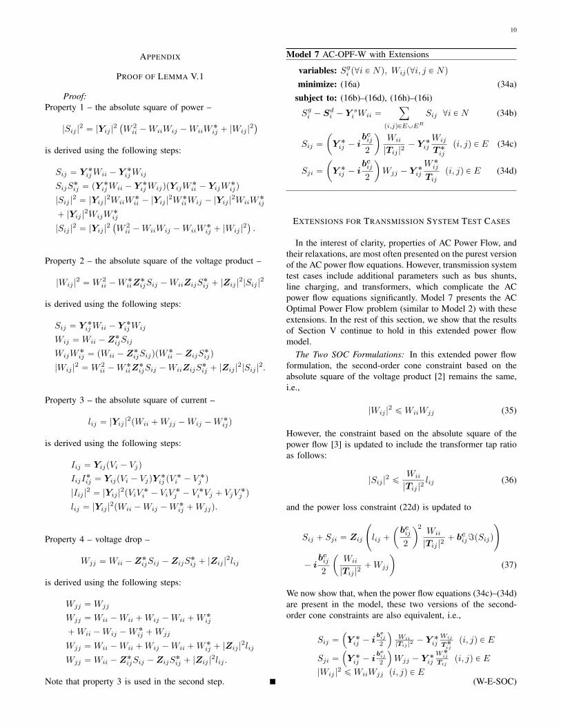
Model 7 AC-OPF-W with Extensions

variables: Sgi p@i P Nq, Wijp@i, j P Nq

minimize: (16a) (34a)subject to: (16b)–(16d), (16h)–(16i)

Sgi ´ Sdi ´ Y

si Wii “

ÿ

pi,jqPEYER

Sij @i P N (34b)

Sij “

ˆ

Y ˚ij ´ ibcij2

˙

Wii

|Tij |2´ Y ˚ij

Wij

T ˚ijpi, jq P E (34c)

Sji “

ˆ

Y ˚ij ´ ibcij2

˙

Wjj ´ Y˚ij

W˚ij

Tijpi, jq P E (34d)

EXTENSIONS FOR TRANSMISSION SYSTEM TEST CASES

In the interest of clarity, properties of AC Power Flow, andtheir relaxations, are most often presented on the purest versionof the AC power flow equations. However, transmission systemtest cases include additional parameters such as bus shunts,line charging, and transformers, which complicate the ACpower flow equations significantly. Model 7 presents the ACOptimal Power Flow problem (similar to Model 2) with theseextensions. In the rest of this section, we show that the resultsof Section V continue to hold in this extended power flowmodel.

The Two SOC Formulations: In this extended power flowformulation, the second-order cone constraint based on theabsolute square of the voltage product [2] remains the same,i.e.,

|Wij |2 ďWiiWjj (35)

However, the constraint based on the absolute square of thepower flow [3] is updated to include the transformer tap ratioas follows:

|Sij |2 ď

Wii

|Tij |2lij (36)

and the power loss constraint (22d) is updated to

Sij ` Sji “ Zij

˜

lij `

ˆ

bcij2

˙2Wii

|Tij |2` bcij=pSijq

¸

´ ibcij2

ˆ

Wii

|Tij |2`Wjj

˙

(37)

We now show that, when the power flow equations (34c)–(34d)are present in the model, these two versions of the second-order cone constraints are also equivalent, i.e.,

Sij “´

Y ˚ij ´ ibcij

2

¯

Wii

|Tij |2´ Y ˚ij

Wij

T ˚ij

pi, jq P E

Sji “´

Y ˚ij ´ ibcij

2

¯

Wjj ´ Y˚ij

W˚ij

Tijpi, jq P E

|Wij |2 ďWiiWjj pi, jq P E

(W-E-SOC)

11

is equivalent to

Sij “´

Y ˚ij ´ ibcij

2

¯

Wii

|Tij |2´ Y ˚ij

Wij

T ˚ij

pi, jq P E

Sji “´

Y ˚ij ´ ibcij

2

¯

Wjj ´ Y˚ij

W˚ij

Tijpi, jq P E

Sij ` Sji “ Zij

ˆ

lij `´

bcij

2

¯2Wii

|Tij |2` bcij=pSijq

˙

´ibcij

2

´

Wii

|Tij |2`Wjj

¯

pi, jq P E

|Sij |2 ď Wii

|Tij |2lij pi, jq P E.

(C-E-SOC)We begin by redeveloping the properties of Lemma V.1 in

the extended model.The Equalities: As both models contain constraints (34c)–

(34d), the properties arising from these equations can betransferred between both models.

Proof:Property 1 – the absolute square of power –

|Sij |2 “ |Yij |

2

˜

W 2ii

|Tij |4´

Wii

|Tij |2Wij

T ˚ij´

Wii

|Tij |2W˚ij

Tij`|Wij |

2

|Tij |2

¸

´

ˆ

bcij2

˙2W 2ii

|Tij |4´ bcij

Wii

|Tij |2=pSijq (38)

The derivation follows similarly to the one presented earlierand the details are left to the reader. The only delicate pointis to observe that three separate terms in the initial expansioncan be collected into =pSijq.

Property 2 – the absolute square of the voltage product –

|Wij |2 “ p1´ bcij=pZijqq

W 2ii

|Tij |2´W˚

iiZ˚ijSij ´WiiZijS

˚ij

` |Zij |2

˜

|Tij |2|Sij |

2 `

ˆ

bcij2

˙2W 2ii

|Tij |2`Wiib

cij=pSijq

¸

(39)

The derivation follows similarly to the one presented earlierand the details are left to the reader.

Property 3 – the absolute square of current –

lij “ |Yij |2

˜

Wii

|Tij |2´Wij

T ˚ij´W˚ij

Tij`Wjj

¸

´

ˆ

bcij2

˙2Wii

|Tij |2´ bcij=pSijq (40)

After observing that the extension of Ohm’s Law in this modelis given by

Iij “

ˆ

Yij ` ibcij2

˙

ViTij

´ YijVj pi, jq P E, (41)

the derivation follows similarly to the one presented earlierand the details are left to the reader.

Property 4 – voltage drop –

Wjj “ p1´ bcij=pZijqq

Wii

|Tij |2´Z˚ijSij ´ZijS

˚ij

` |Zij |2

˜

lij `

ˆ

bcij2

˙2Wii

|Tij |2` bcij=pSijq

¸

(42)

The proof follows similarly to the one presented earlier andthe details are left to the reader.

With these core properties updated, we are now ready to extendthe proof from Section V.

Theorem A.1. (C-E-SOC) is equivalent to (W-E-SOC).

Proof:

The proof follows the one presented in Section V.

a) W-E-SOCñ C-E-SOC: Every solution to (W-E-SOC)is a solution to (C-E-SOC). Given a solution to (W-SOC), byequality (3), we assign lij as follows:

lij “ |Yij |2

˜

Wii

|Tij |2´Wij

T ˚ij´W˚ij

Tij`Wjj

¸

´

ˆ

bcij2

˙2Wii

|Tij |2´ bcij=pSijq pi, jq P E (43)

This assignment satisfies the power loss constraint (37) bydefinition of the power. It remains to show that second-ordercone constraint in (C-E-SOC) is satisfied. Using equalities (1)and (3), we obtain

|Sij |2 “ |Yij |

2

˜

W 2ii

|Tij |4´

Wii

|Tij |2Wij

T ˚ij´

Wii

|Tij |2W˚ij

Tij`|Wij |

2

|Tij |2

¸

´

ˆ

bcij2

˙2W 2ii

|Tij |4´ bcij

Wii

|Tij |2=pSijq (44a)

|Sij |2 ď |Yij |

2

˜

W 2ii

|Tij |4´

Wii

|Tij |2Wij

T ˚ij´

Wii

|Tij |2W˚ij

Tij`WiiWjj

|Tij |2

¸

´

ˆ

bcij2

˙2W 2ii

|Tij |4´ bcij

Wii

|Tij |2=pSijq (44b)

|Sij |2 ď

Wii

|Tij |2

˜

|Yij |2

˜

Wii

|Tij |2´Wij

T ˚ij´W˚ij

Tij`Wjj

¸¸

´Wii

|Tij |2

˜

ˆ

bcij2

˙2Wii

|Tij |2´ bcij=pSijq

¸

(44c)

|Sij |2 ď

Wii

|Tij |2lij . (44d)

b) C-E-SOC ñ W-E-SOC: Every solution to (C-E-SOC)is a solution to (W-E-SOC). We show that the values ofWij in (C-E-SOC) satisfy the second-order cone constraintin (W-E-SOC). Using equalities (2) and (4) and the fact that

12

1e−01 1e+01 1e+03

020

4060

8010

0

Time (log, seconds)

Num

ber

of In

stan

ces

Sol

ved

W−SOCC−SOC

Fig. 3. Runtime Profiles for the Two SOC Relaxations.

Wii “W˚ii since Wii is a real number, we have

|Wij |2 “ p1´ bcij=pZijqq

W 2ii

|Tij |2´W˚

iiZ˚ijSij ´WiiZijS

˚ij

` |Zij |2

˜

|Tij |2|Sij |

2 `

ˆ

bcij2

˙2W 2ii

|Tij |2`Wiib

cij=pSijq

¸

(45a)

|Wij |2 ď p1´ bcij=pZijqq

W 2ii

|Tij |2´W˚

iiZ˚ijSij ´WiiZijS

˚ij

` |Zij |2

˜

Wiilij `

ˆ

bcij2

˙2W 2ii

|Tij |2`Wiib

cij=pSijq

¸

(45b)

|Wij |2 ďWii

ˆ

p1´ bcij=pZijqqWii

|Tij |2´Z˚ijSij ´ZijS

˚ij

˙

`Wii

˜

|Zij |2

˜

lij `

ˆ

bcij2

˙2Wii

|Tij |2` bcij=pSijq

¸¸

(45c)

|Wij |2 ďWiiWjj (45d)

and the result follows.

Corollary A.2. Model 5 is equivalent to Model 6 in theextended AC Power Flow formulation from Model 7.

COMPARISON OF SOC FORMULATIONS

Section V proposed two equivalent formulations of thesecond-order cone constraints for power flow relaxations.Although both formulations define the same convex set, it isunclear if they have the same performance characteristics. Forexample, the current-based constraint (C-SOC) has more con-straints and more variables than the voltage-product constraint(W-SOC). All other aspects being equal, one would expect(C-SOC) to be slower than (W-SOC). This section investigatesthe performance implications of these two formulations onboth the QC and SOC power flow relaxations. Four powerflow relaxations are considered, W-SOC (Model 4), C-SOC(Model 4 with (C-SOC)), W-QC (Model 5 with (W-SOC)), andC-QC (Model 5). To test the performance of these relaxations,each model is evaluated on 105 state-of-the-art AC-OPF

1e−01 1e+01 1e+03

020

4060

8010

0

Time (log, seconds)

Num

ber

of In

stan

ces

Sol

ved

W−SOCC−SOC

Fig. 4. Runtime Profiles for the Two QC Relaxations.

transmission system test cases from the NESTA v0.4.0 archive[35]. Figure 3 compares the two variants of the SOC relaxationand Figure 4 compares two variants on the QC relaxation.

Both figures indicate that the two formulations are verysimilar for small test cases but, on the larger test cases (i.e.,with more than 1000 buses), the C-QC formulation has a fasterconvergence rate, in IPOPT. This suggests that, despite itsincreased size, the C-QC formulation originally presented in[4] is preferable from a performance standpoint and that theC-SOC formulation may be preferable on very large networks(e.g. above 9000 buses).