Technical Series Paper #99-02

The PSID and Me

Greg J. Duncan Northwestern University

School of Education and Social Policy

and

Faculty Fellow, Institute for Policy Research

April 18, 1999

This project was supported by funding from the National Science Foundation (SES 9515005).

WP-99-14

The PSID and Me

Greg J. DuncanNorthwestern University

School of Education and Social Policyand

Faculty FellowInstitute for Policy Research

The PSID and Me

Greg J. DuncanNorthwestern University

April 18, 1999

Prepared for the Murray Research Center Conference “Landmark Studies of the TwentiethCentury”, to be held April 23-24, 1999. This paper benefited from comments by DorothyDuncan, Rachel Dunifon, Martha Hill, John Modell, and James Morgan.

AbstractI begin with a brief history of the Panel Study of Income Dynamics (PSID) and its

brilliant founding father, noting its nearly disastrous initial design, nearly fatal funding cutoffswhen Nixon put the Office of Economic Opportunity out of business, and then when Reaganchopped the NSF social science budget in half, and paying honor to its exceptionally talented,long-lived and unsung staff.

Since it is impossible to cover all of the lessons learned from the PSID, I concentrate onwhat is of greatest interest to me: the surprising degree of economic mobility in the U.S. – bothwithin and between generations, with its attendant implications for understanding the nature anddevelopmental consequences of life cycle processes in general, and poverty and welfaredynamics in particular.

As of four years ago, when I left the PSID and Michigan for Northwestern, I had spenthalf my life working on the PSID. Not surprisingly, my PSID phase has had a profound effect onmy life. The recognition that economic fortunes bob around on a sea of demographic change ledto my interest in determinants and sequelae of family composition changes. The heterogeneousnature of poverty and welfare receipt – frequently transitory but a worrisome amount persistent –stimulated my interest in understanding their consequences for children’s development. Pursuingthese interests has led to many interdisciplinary collaborations, a chance meeting at an airport 17years ago with the woman who is now my wife and, in 1995, a change of jobs and disciplinaryaffiliation.

The PSID and Me

Since I was a Grinnell College sophomore when the Panel Study of Income Dynamics

(PSID) began, I can claim no credit for its remarkable design or early history. I began working

on the project in its fifth and, according to the original plan, final year.

Now thirty years old, the PSID continues to collect data from its loyal but ever-changing

national sample of families. These data have been the basis of dozens of dissertations and

hundreds of articles. Taken together, the study’s data have forced us to confront and learn from

the dynamism inherent in economic and demographic processes.

Now fifty years old, I am no longer associated with the study but continue to follow the

trajectories begun when I was part of the PSID. I seek in this paper to describe the study and my

relationship to it. I begin with a brief history of the PSID, followed by a summary of some of the

more important lessons learned from it. Throughout I mix project and personal history and show

how my 23 years with the project, and four years since, have shaped my career and life.

THE STUDY ITSELF

As part of Lyndon Johnson's War on Poverty, the Office of Economic Opportunity

(OEO) directed the U.S. Bureau of the Census to conduct a nationwide assessment of the extent

to which the War on Poverty was affecting people's economic well-being. This Census Bureau

study, called the Survey of Economic Opportunity (SEO), completed interviews with about

30,000 households, first in 1966, and again in 1967.

Interest in continuing this survey of economic “trajectories” (the other war going on at

the time contributed its share of metaphors to the poverty debate), but avoiding Census Bureau

bureaucracy, led James D. Smith and his OEO colleagues to approach James Morgan at the

Survey Research Center (SRC) at the University of Michigan about interviewing for five years a

nationally representative subsample of approximately 2,000 low-income SEO households. With

extensive prior experience in economic surveys, an ability to endear himself to sponsors by

generating and then returning budget surpluses, co-authorship of the remarkably

underappreciated 1961 book Income and Welfare in the United States, an unlimited supply of

3

bright ideas, bad puns and funny phrases, and paternal genes inherited from a Ph.D. psychologist

who wrote How to Keep a Sound Mind, Morgan, a Professor of Economics and Program

Director at SRC, was a natural choice to lead the new study.

Morgan, however, was initially reluctant to take it on because the seriously flawed OEO

design called for following only low-income households.1 Arguing the formidable virtues of

complete population representation, pointing out, for example, that understanding why nonpoor

households fell into poverty was at least as interesting as knowing why poor households climbed

out, Morgan was successful in talking OEO into funding a design in which 2,000 randomly

chosen initially-poor OEO households were combined with a fresh cross-section of about 3,000

households from the SRC national sampling frame.2 When weighted, the combined sample was

representative of the entire population of the United States, including non-poor as well as poor

households. But the disproportionately large number of low-income households produces large

analysis samples for black and other disadvantaged groups.

The year 1972 proved momentous for the PSID. Its original five years were coming to an

end and, dramatically, then-President Nixon abolished the OEO virtually overnight.

Responsibility for the PSID was transferred to the Assistant Secretary for Planning and

Evaluation (ASPE) of the Department of Health, Education and Welfare (now Health and

Human Services) where visionary ASPE officials such as Larry Orr saw the value of continuing

to support the PSID.3

1 Morgan also feared OEO micromanagement. But micromanagement proved impossible foroverburdened OEO staff and the PSID enjoyed its own form of benign neglect.

2 Throughout this career, Morgan has responded to requests to perform proposed surveys with details oncreative study designs that, in his often firmly-stated opinions, the sponsors should have adopted. Itworked in the case of the PSID but rarely afterward.

3 In personal communication, Larry Orr provided the following story of his behind-the-scenesmaneuvering at ASPE: “At some point in the mid-70s, it looked like the Contracts Office was finallylosing patience with our annual non-competitive extensions of the contract and was going to make uscompete it. We were also starting to get some flak from the other parts of ASPE, who were askingwhether this thing was worth the large chunk of the Policy Research budget that it was consuming. So Iconvened a blue-ribbon panel of folks I knew would be sympathetic to the project (and to Michigan'scontinued stewardship of it) and got a report saying that this should be just behind the Washington

4

The year 1972 was also my first with the project. As a second-year economics graduate

student at Michigan, I was attracted to work at the Survey Research Center by Morgan’s mile-a-

minute course on survey methods and by the invaluable experience of spending my senior

undergraduate year in Costa Rica as part of a field studies program. My research project focused

on how efficiently Costa Rican farmers, truckers, and wholesalers brought to market basic

agricultural produce. I conducted and analyzed data from interviews throughout the country.

Fortunately, the data I collected over the course of my year in Costa Rica were much better

behaved than I was.

I loved working on the PSID project and at the Survey Research Center. My first tour of

duty was as a data editor, reading the often lengthy interviewer explanations of complications

that rendered responses to the PSID’s many closed-ended questions problematic, making sense

of the demographic and economic data, observing the myriad events behind families’ seemingly

tumultuous economic fortunes, and learning which pieces of data deserved the greatest trust.

Morgan’ s first quantitative analysis assignment for me was to use as many as necessary

of the 2,978 variables gathered over the course of the first five years of the study to understand

responses to the fifth-year open-ended question: “We have been visiting you for five years now

and asking a lot of questions, but we are also interested in your overall impression of this period.

How would you say things have gone for you during the last five years?” Sobering in the

responses were precious few references to earnings, capitalist exploitation, family income, class

solidarity or another of the other economic and class factors I championed at the time. And

almost nothing in the PSID’s wealth of variables accounted for differences in reports of either

the level or trends in well-being revealed by these open-ended responses. More generally, the

assignment was hopelessly beyond my capabilities, but the process of flailing through data and

literature planted a number of seeds in my mind that would later sprout.

Other, more manageable, analyses led to chapters published in the first of ten Five

Thousand American Families volumes and my first journal articles. With time, my work on the

monument on the government's list of national treasures. It worked, and from that point on, thecontinuation of the survey was, as I recall, pretty much a non-issue.”

5

PSID came to include questionnaire development and proposal writing for future waves, and

helping to manage many of the other tasks associated with an annual panel survey.

Equally stimulating was the enterprise of the Survey Research Center itself. Dependent

for 95% of its budget on the research-grant “overhead” it generated, SRC had developed a strong

set of community-building norms, a sense of shared fate, and democratic decision-making. Its

periodic staff lunches and, with time, some research collaborations reinforced my appreciation

for the value of work going on in other disciplines. The dignity and wisdom with which

researchers such as Angus Campbell, Robert Kahn and Leslie Kish conducted themselves, their

research, and, when called upon, their administrative duties, left a deep impression on me. I

gained my Ph.D. in 1974 and garnered a few job offers but found the option of staying with the

PSID was much more compelling - and indeed I remained with the study for the next twenty

years.

By the late 1970s, after a decade of operation, the PSID’s status properly evolved from a

“poverty study” into a unique longitudinal data resource for social scientists from several

disciplines. This, combined with ASPE’s declining budget fortunes, led to a transfer of primary

funding for the study from ASPE to the National Science Foundation. Ronald Reagan’s attempt

to all but eliminate social science research from the National Science Foundation budget in the

early 1980s would have done in the PSID, had it not been for three years of emergency funding,

orchestrated by Tom Juster, from the Ford, Sloan and Rockefeller Foundations.

The intellectual agenda of the PSID’s data collection has always been two-fold. The first

is to maintain a clean and consistent time series of core content - employment, family income

and family structure – based on the study’s annual interviews. The second, dictated by our desire

to maintain the PSID’s capacity to address contemporary research issues and, eventually, by the

funding structure of the study, has been to complement the core with question supplements.

The poverty focus of the PSID’s early years led to the inclusion of an eclectic set of

supplemental measures that might be expected to differentiate families that climbed out of

poverty from those who stayed poor. Thus, the first five annual questionnaires are filled with

measures of locus of control, future orientation, achievement motivation, employment barriers,

entrepreneurial activity, trust/hostility, avoidance of unnecessary risks, access to sources of

6

information and help, and a short sentence-completion test. As explained in the final section of

this paper, some of the measures have proved quite powerful in differentiating individuals

according to their long- (but not short-)run successes and failures.

The surge of labor-market research in the 1970s led us4 to eliminate the PSID’s gender

bias in the detail of questions asked of married women and to add interesting question

supplements on work histories, labor-market attachment and on-the-job training. In 1980,

Morgan anticipated the interest in “social capital” by leading an effort to develop a question

supplement on both past and possible future flows of time and money help between households.

These were exciting times, since we had the freedom to conceive and develop supplements on

contemporary topics which, when coupled with the PSID’s ever-expanding time series of core

content, would provide us and a growing national network of analysts with unique data drawn

from our large national sample of households.

The nature of PSID’s operations changed somewhat when its major funding was taken

over in the early 1980s by the National Science Foundation. A Board of Overseers began to

review and pass judgment on PSID operations. While many of their suggestions have improved

the PSID considerably, the burdens of dealing with academic overseers proved considerable.5

The creative elements of the PSID shifted more and more to the invention and design of question

modules that supplemented the PSID’s demographic and economic core. Since NSF never

funded more than 70% of what it took to collect and process the data, we became much more

dependent on Federal agencies and, occasionally, private foundations to fund question

supplements that would help cover the PSID’s $2.5 million (current dollar) annual cost.

Substantively, the question supplements developed in the 1980s and early 1990s and

funded primarily by the National Institute of Child Health and Human Development and the

National Institute on Aging enabled the PSID to add many valuable question supplements on

4 Mary Corcoran, Martha Hill and Karen Mason spearheaded the effort to establish comparabilitybetween the labor market information collected from men and women.

5 As NSF funding increased, the PSID Advisory Board became the PSID Board of Overseers. Oneprominent member sent a letter to us shortly after the change, making sure that we understood the changewas more than semantic!

7

fertility, health, wealth, child development and intergenerational transfers, as well as a Ford-

Foundation-funded supplement sample of Latino households. We also found funding for projects

establishing links between PSID sample members and the National Death Index and between

PSID respondent addresses every year and geographic identifiers such as census tracts, ZipCodes

and counties, which has enabled analysts to match contextual information from the decennial

census and other sources to the interview information to explore the nature of neighborhood

effects.

Operationally, these supplemental activities required a great deal of proposal writing and

other entrepreneurial effort, much of which I assumed when I joined Morgan as the study’s co-

director in 1982. Although burdensome,6 the process forced me to come up to speed on many

topics that would eventually become part of my research and develop a network of contacts in

government agencies. Reducing the burden during this period were an invaluable set of

colleagues, in particular Martha Hill, Dan Hill, Charlie Brown and Jim Lepkowski, and a

remarkably capable and perceptive set of individuals working in the government agencies, in

particular Daniel Newlon in the NSF, Jeffrey Evans in NICHD and Richard Suzman in NIA, all

of whom understood both the research issues and how to work their bureaucracies to secure the

needed money. I was joined in 1993 by co-director Sandra Hofferth, who, with Frank Stafford, is

the principal investigator of the PSID today.

A final set of burdens, which figured in to my willingness to leave the PSID in 1994,

began in 1992 when the NSF determined that PSID interviewing needed to be switched from

paper-and-pencil to computer-assisted methods. This change was recommended by individuals

who had enjoyed great success implementing computer-assisted interviewing methods in cross-

sectional surveys. Converting the PSID to computer-assisted methods was a nightmare, since we

6 Our typical situation had us preparing to release data gathered two years before, cleaning data collectedone year before, attending to response rates and costs of the current round of data collection, pretestingquestions for the following year and writing proposals for possible question supplements two and threeyears hence. The highlight of these burdens for me was spending an Easter weekend in the late 1980swriting a proposal to the National Science Foundation that justified why the PSID was THE study forunderstanding the economic and social consequence of global warming! It seems that a NSF global-warming initiative provided the social science divisions with an opportunity to substitute that initiative’sfunds for others.

8

wanted to avoid creating a “seam” in the PSID’s long time-series, had very complicated family-

relationship question sequences and faced situations every year in which newly-formed families

that were discovered during the interviewing process needed to be contacted and interviewed.

None of these tasks could be accommodated with existing software. Our costs failed to fall as

advertised; our careful hand-editing of the data was eliminated in favor of much less satisfactory

questionnaire-related programming; a programmer became part of the delicate questionnaire

design process and the lead time needed to develop the next year’s questionnaire increased by

several months. At least when it comes to inserting technology into an ongoing panel study, I am

most decidedly a Luddite.

SOME IMPORTANT LESSONS FROM THE PSID

Fundamental to the success of the PSID are the often-overlooked advantages of

following, and keeping as part of the sample, members of the families who moved away from

their original households to set up new households, such as children who came of age during the

study (Hill, 1992). Since such individuals were originally chosen to be representative of the

general U.S. population, the new families they form in the PSID sample are themselves

representative of new families formed in the larger U.S. population.7 Furthermore, since children

born to the PSID’s representative sample families are themselves a representative sample of

children, the study’s design also provides continuous representation of births.

When played out over 30 years, these design features enable the PSID to provide: i) data

on representative cross-sections of families and individuals in 1968; ii) data on representative

annual cross-sections of families and individuals between 1969 and 1997; iii) 30-year

longitudinal data on individuals in the initially-representative 1968 sample, including children

observed both when they were living with their parents and long after striking out on their own

in adulthood; and iv) shorter-run comparative longitudinal data on representative cohorts of

individuals at any point between 1968 and 1997.

7 An exception is new U.S. families formed through immigration, which have no chance of entering astudy like the PSID. Immigrant samples were added to the PSID in 1990 and 1997.

9

Four other crucial design features of the PSID are that the core content of the study’s

annual interviews has remained largely unchanged; response rates have been high and largely

random (Fitzgerald et al., 1998); remarkable effort has been expended on cleaning the data in

exactly the same way in virtually every year of the study;8 and data have always been released to

the larger research community as soon as they are cleaned and documented. Unplanned but

inevitable given the stimulating and supportive environment Morgan created and I tried to

maintain is the fact that many key support staff have remained with the study for decades.

It is impossible to overemphasize the key role played by support staff in the success of

the study. Collectively, they provided the institutional memory needed to keep the data

comparable across waves. And in their individual ways, they quickly discovered optimal

methods for persuading reluctant respondents to continue with the study, wrote questions that

normal (i.e., non-academic) people understood, processed the data and counseled the horde of at

times irritating young researchers outside of SRC who wanted to use the data but sometimes, in a

few memorable cases, refused to read even the first page of documentation. Their perfectionism

caused more than a few headaches in meeting deadlines, but their single-minded dedication to

getting things right has produced an extraordinarily detailed and accurate motion picture of

American economic family life in the last third of the twentieth century.

These features have made the PSID one of the most widely used and influential data sets

in the social science research community. As of 1996, PSID-based articles have appeared in over

100 different refereed journals; the bibliography lists some 1,200 publications in all. In the early

8 Data “editing,” my first job with the PSID, consisted of a 45-minute-per-completed-interviewexamination of questionnaire responses as well as interviewer comments by a trained data editor,following detailed and unchanging rules, to produce an unusually clean and, across waves, consistent setof key family and economic variables. Over the course of my 23 years with the PSID I had manyoccasions to visit the paper questionnaires stored in the subbasement of the Institute for Social Researchin order to make sense out of what appeared from my analyses to be erroneously-coded data. Invariably,the problem was with my inability to anticipate the complexities of family economic life; I found virtuallyno editing or coding errors. The data-cleaning operation changed considerably when computer-assistedinterviewing techniques were introduced in 1993.

10

1990s, publication rates were five per year in the top four economics journals, six per year in the

top labor-economics journals, and five per year in the top five sociology and family journals.9

I cannot hope to present a comprehensive summary of what has been learned from these

many studies. In the spirit of the conference, my approach is decidedly selective and personal.

What a family’s “life cycle” is really like

Despite the study’s longitudinal nature, most analysts, myself included, typically

approached the PSID’s first decade of data as though they were drawn from a cross section.

Longitudinal methods were not well developed in the 1970s, and the PSID questionnaire

provided many novel measures that, when analyzed using cross-sectional methods, produced

interesting and, most importantly, publishable articles. My own studies were inspired by my

training as a labor economist and focused on then-popular topics such as earnings differences

between men and women and between union and nonunion workers, economic rewards of on-

the-job training, childcare choices of working parents, and, using retrospective reports,

intergenerational models of completed schooling.

Lurking in the background, however, were persistently puzzling PSID data suggesting a

striking degree of economic turbulence and perhaps genuine mobility at all income levels

(Morgan et al., 1974; Duncan et al., 1984). Incomes fluctuated a great deal from one year to the

next, producing many transitions into and out of both poverty and affluence, and onto and off the

welfare rolls. Moreover, other important changes frequently took place: roughly one in five

families changed composition from one year to the next and a comparable fraction pulled up

stakes and moved from one location to another.

What was going on? Were the income changes merely the result of measurement errors,

or were families’ economic fortunes really more volatile than previously believed? If the

turbulence was real, what caused it and to what extent was it voluntary or at least anticipated?

And how much of the turbulence reflected true mobility – permanent changes in economic and,

perhaps, social position?

9 These publication data come from the PSID’s 1996 proposal to the National Science Foundation.

11

The prevalent academic conceptions of social and economic position in the 1970s were of

unchanging social class; slowly building stocks of economically valuable (human capital) skills;

or fairly predictable life-cycle changes experienced by individuals as they age. In the life-cycle

view, early adulthood is usually seen as a period of relatively low income as career and marital

arrangements are being sorted out. Income grows as careers stabilize and, in some cases,

blossom, and as multiple earners in households increase the household's total income. Retirement

usually occasions a drop in income, cushioned by social security and private pension payments

in both nominal income and work-related expenses.

Lenore Weitzman’s (1985) sensational but erroneously overstated depiction of the dire

economic consequences of divorce was still years in the future and had not yet been integrated

into life-cycle theories. Elder’s landmark studies of the Great Depression (1974) provided a vivid

picture of the consequences of severe macroeconomic disruptions, but few thought that these

kinds of disruptions were a regular feature of many families’ lives in the prosperous second half

of the 20th century.

This life-cycle view of income changes conforms closely to (and, indeed, has been

developed from) family-income data drawn from representative cross-sections of the population

showing higher levels of household income for older individuals until the late 40s, and then

lower levels at older ages. If we succumb to the temptation to use these cross-sectional data on

different families at various life cycle stages to represent the likely economic path of individuals

as they age, then we might view individual income trajectories as fairly smooth, with fluctuations

occurring infrequently and at discrete points of the life cycle such as early adulthood and

retirement.

PSID as well as subsequent longitudinal household and administrative data reveal

economic and social trajectories that are much more disparate and chaotic than envisioned by a

life-cycle view. An idea of the scope of these fluctuations can be gleaned from Table 1, which is

taken from Duncan’s (1988) PSID-based analysis of household income trajectories over the

12

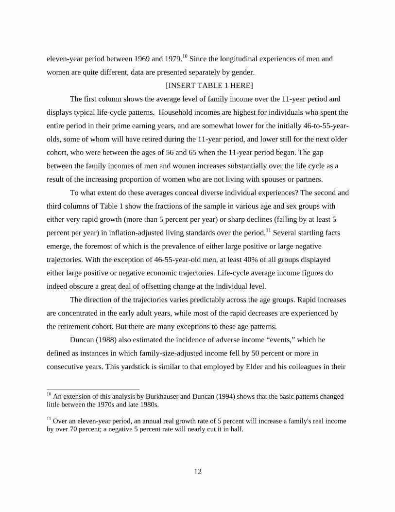
eleven-year period between 1969 and 1979.10 Since the longitudinal experiences of men and

women are quite different, data are presented separately by gender.

[INSERT TABLE 1 HERE]

The first column shows the average level of family income over the 11-year period and

displays typical life-cycle patterns. Household incomes are highest for individuals who spent the

entire period in their prime earning years, and are somewhat lower for the initially 46-to-55-year-

olds, some of whom will have retired during the 11-year period, and lower still for the next older

cohort, who were between the ages of 56 and 65 when the 11-year period began. The gap

between the family incomes of men and women increases substantially over the life cycle as a

result of the increasing proportion of women who are not living with spouses or partners.

To what extent do these averages conceal diverse individual experiences? The second and

third columns of Table 1 show the fractions of the sample in various age and sex groups with

either very rapid growth (more than 5 percent per year) or sharp declines (falling by at least 5

percent per year) in inflation-adjusted living standards over the period.11 Several startling facts

emerge, the foremost of which is the prevalence of either large positive or large negative

trajectories. With the exception of 46-55-year-old men, at least 40% of all groups displayed

either large positive or negative economic trajectories. Life-cycle average income figures do

indeed obscure a great deal of offsetting change at the individual level.

The direction of the trajectories varies predictably across the age groups. Rapid increases

are concentrated in the early adult years, while most of the rapid decreases are experienced by

the retirement cohort. But there are many exceptions to these age patterns.

Duncan (1988) also estimated the incidence of adverse income “events,” which he

defined as instances in which family-size-adjusted income fell by 50 percent or more in

consecutive years. This yardstick is similar to that employed by Elder and his colleagues in their

10 An extension of this analysis by Burkhauser and Duncan (1994) shows that the basic patterns changedlittle between the 1970s and late 1980s.

11 Over an eleven-year period, an annual real growth rate of 5 percent will increase a family's real incomeby over 70 percent; a negative 5 percent rate will nearly cut it in half.

13

studies of the effects of the Great Depression, which found long-lasting effects of income drops

of one-third or more.

The incidence of sharp drops in income-to-needs over the life course is shown in the

fourth column of Table 1. The overall risk is high: between 18% and 39% of the various groups

are estimated to have experienced such a drop at least once during the eleven-year period. Most

of these decreases left the individuals involved with, at best, modest incomes. Not shown in

Table 1 is the fact that 87% of the individuals experiencing these decreases saw their family

incomes fall to less than $25,000.

Since the PSID questions respondents about their expectations of future changes in

economic status,12 it is possible to calculate what fraction of the 50%+ income drops were

preceded in either of the previous two annual interviews by a report that the respondent expected

his or her family economic status to decline. The fifth column of Table 1 shows that a majority

of all income declines and the vast majority of pre-retirement income drops were unexpected.

Taken together, longitudinal PSID data show that it is a mistake to treat the “path” of

average incomes as the typical income course of individuals as they age. Family incomes are

quite volatile at nearly every point in the life cycle, making rapid growth or decline in living

standards more the rule than the exception. We do not have to look with Elder and his colleagues

to the Great Depression to find frequent instances of economic loss and hardship; the risk of

sharp decreases in living standards is still significant at virtually every stage of life. Most of the

losses are unexpected. These losses occur despite our system of government safeguards

(unemployment insurance, Aid to Families With Dependent Children) and intrafamily transfers

that might be expected to reduce or eliminate them.

So what?

Should these newly-discovered economic fluctuations be a concern? Elder’s data provide

compelling but historical evidence of circumstances in which economic shocks can have

12 After a sequence of other questions about household income, respondents were asked "What about thenext few years, do you think you will be better off, or worse off, or what?"

14

devastating effects on both adults and children. In Falling From Grace, (1988) Katherine

Newman draws data from the 1980s to document the psychological and other damage brought

about by downsizing, divorce and other events. Countless more specialized studies focus on the

consequences of individual events such as layoffs, divorce and widowhood. Perhaps

contemporary economic dislocations are even more damaging than those in the 1930s, since

there is much less of a sense that these events are shared by others.

On the other hand, some events producing economic losses may have benign or even

beneficial effects. Children leave parental homes and older parents decide not to move in with

their adult children, despite economic advantages they would otherwise enjoy, because they

value their independence. Although their incomes are lower than before retirement, retired

individuals may be better off because they have more leisure time than when they were working,

and the predictability of retirement has allowed them time to prepare for its financial and

psychological consequences. Despite their unstable incomes, construction workers may be well

off because their higher rates of pay compensate them for the instability of their jobs, while the

self-employed may value “being their own bosses” over a stable salary. In short, not all instances

of income instability have the same negative implications. Indeed, some have argued explicitly

that income variability over the life cycle is of little analytic and policy interest (Murray, 1986).

Research on the consequences of economic fluctuations is difficult because few data sets

combine reliable longitudinal information on family income with well-measured subsequent

physiological or psychological outcomes. An interesting exception using PSID data related the

level and stability of income to mortality (McDonough, Duncan, et al., 1997). They treat PSID

data as if they were a series of independent 6-year panels, the first spanning calendar years 1972-

78, the second spanning 1973-79, and so forth, with the last one spanning the decade from 1983-

1989. Within each six-year period they use the first five years to measure the level and stability

of household income and the sixth and final year to measure possible mortality.

Key results are presented in Table 2. They are taken from a logistic regression in which

the dependent variable is whether the individual died during the sixth and final year of the given

period. Income level and stability over the five-year period preceding the possible death are

combined into a single classification of: i) low and unstable income (i.e., mean income under

15

$20,000 and at least one big income drop13 over the given five-year period; ii) low but stable

income; iii) middle-class (mean income between $20,000 and $70,000) and unstable; iv) middle-

class and stable; v) affluent and unstable. Affluent individuals with stable incomes served as the

reference group.14

[INSERT TABLE 2 HERE]

Consistent with a number of other studies, mortality risks fall with income level.

Individuals with low incomes have 3 to 4 times the mortality risk of the affluent individuals in

the reference group. New in the analysis is the result that unstable incomes also contribute to

mortality risk, but only among the middle class. When compared with the consistently-affluent

reference group, middle-income individuals with stable incomes had a marginally significant

1.5-times elevation of mortality risk. In contrast, an individual with middle-class but unstable

income had a risk ratio more than three times that of individuals in the reference group, and

almost as high as individuals in the two low-income groups. Instability mattered neither at the

low nor high end of the income distribution, perhaps because the disadvantages of low incomes

and the advantages of affluence overwhelm the possible effects of instability. An important item

for future research is whether it is the income fluctuations per se or the events (e.g.,

unemployment, widowhood) producing them that increase the mortality risks.

Poverty and welfare dynamics

Published in 1984, the book Years of Poverty, Years of Plenty was an attempt by me and

my coauthors to summarize the most important lessons from the first ten years of the PSID.15 It

included chapters on family economic and labor-market mobility, labor market differences

between blacks and whites and between men and women, and poverty and welfare dynamics. We

13 Consistent with Table 1, an income drop is defined as a situation in which size-adjusted family incomefell by 50% or more in consecutive years.

14 Control variables include age of individual, calendar year, race, and the average size of the givenperson's household over the first five years of the window.

15 The coauthors – Morgan, Richard Coe, Martha Hill, Saul Hoffman, Mary Corcoran – were cherishedcollaborators in my first years with the PSID.

16

wrote it to be an accessible summary of findings and were pleased by the extent to which it

found its way into classrooms and policy discussions.

The interest generated by the book focused overwhelmingly on its findings on the

dynamic nature of poverty and welfare use. As with the more general life-cycle results, there was

a huge gap between popular perceptions of these phenomena and the data’s clear message of

turbulence and mobility. When the PSID began, and continuing today, popular perceptions of the

permanence of poverty and welfare receipt are widespread. We speak easily of “the poor” as if

they were an ever-present and unchanging group. Indeed, the way we conceptualize the “poverty

problem,” the “underclass problem” or “the welfare problem” seems to presume the permanent

existence of well-defined groups within American society.

Much of our data on poverty is based on large annual Census Bureau surveys in which

family annual cash incomes are compared with a set of “poverty thresholds” that vary with

family size. In 1998, a three-person family with an income below $12,802 would be designated

as poor; the threshold for a four-person family is $16,400. Although the poverty rates calculated

each year by the Census Bureau generate a great deal of publicity, they rarely change by as much

as a single percentage point from one year to the next. Longer-run trends show jumps during

recessions and a disturbing secular increase in the poverty rate among families with children.

Evidence that, say, one in five children was poor in two consecutive Census-Bureau

survey “snapshots,” and that those poor children shared similar characteristics (e.g., half lived in

mother-only families) is consistent with an inference of absolutely no turnover in the poverty

population and seems to fit the stereotype that poor families with children are likely to remain

poor, and that there is a hard-core population of poor families with little hope of self-

improvement. However, the same evidence is equally consistent with 100 percent turnover – or

any other percentage one might pick – assuming only that equal numbers of people with similar

characteristics cross into and out of poverty.

In fact, longitudinal data from the PSID have always revealed a great deal of turnover

among both the poor and welfare recipients (Duncan et al., 1984). Only a little over half of the

individuals living in poverty in one year are found to be poor in the next, and considerably less

17

than one-half of those who experience poverty remain persistently poor over many years.

Similarly, many families receive income from welfare sources at least occasionally, but

relatively very few do so year after year.

Many descriptions of poverty experiences are possible with the PSID; perhaps the

simplest is a count of the number of years in which an individual lived in a family with total

annual income that fell short of the poverty threshold in that year. In the case of the eleven-year

period used for Table 1, if poverty were a persistent condition, then the sample would cluster at

one of two points -- no poverty at all or poverty in all of the eleven years. If much contact with

poverty is occasional, then we would expect that the persistently poor would be a small subset of

the larger group that had at least some experience with poverty.

The last two columns of Table 1 show what fractions of individuals in the various

age-sex groups spent at least one of the eleven years below the poverty line and those who spent

more than half of the time (at least six of eleven years) in poverty.

The difference in the sizes of these two groups at all stages of the life cycle is striking.

Depending on the life-cycle stage, between 20% and 27% of adult women experienced poverty

at least once during the eleven-year period. The risk of at least occasional poverty was

considerably lower for adult men than women. Persistent poverty, defined as living in poverty

for more than half of the eleven-year period, characterized fewer than one-tenth of any of the

subgroups. An older woman's chance of experiencing persistent poverty was roughly twice that

of a 25-44-year-old woman and nearly five times as high as that of a 25-44-year-old man.

Poverty rates for children and, especially, minority children are much higher, with nearly one-

quarter of black children living in persistent poverty (U.S. Department of Health and Human

Services, 1997).

By adopting “event history” methods such as the life table and Cox regression (Tuma and

Groeneveld, 1979), Mary Jo Bane and David Ellwood (1986, 1994) furthered the transformation

in how social scientists and policy analysts viewed poverty and welfare dynamics. These

methods enabled them to characterize the nature and determinants of poverty and welfare

experiences by the length of their “spells” (i.e., continuous periods of poverty or receipt).

18

Essential data from the Bane and Ellwood analyses are presented in Table 3. In the case

of poverty, they use the PSID to estimate what fraction of families who first begin a poverty

experience do so for short (i.e., 1-2 years), medium (3-7 years) and longer-run (8 or more years)

periods of time. They find that while a clear majority of poverty spells are short, a substantial

subset of poor families have longer-run experiences. Heterogeneity of experiences is thus key.

Striving to discover THE correct characterization of poverty - transitory or persistent - is

fruitless, since poverty experiences are always a mixture of transitory and long-term. The policy

implications of these data are profound, since the heterogeneous nature of poverty experiences

demands a heterogeneous set of policies to address the needs they create. The short-term needs

associated with short spells call for social-insurance approaches in which fears of “dependence”

need not be a concern. Long-term poverty spells are a different matter, and call for policies that

address the causes of the longer-run problems of the poor.

In the data presented in the second column of Table 3, Bane and Ellwood (1994)

calculate the likely total number of years of receipt for families just starting to receive Aid to

Families With Dependent Children (AFDC).16 They find a roughly even distribution of first-time

welfare recipients across the three time intervals; roughly one-third have very short welfare

experiences, a third medium-length experiences and the final third long-term receipt.

[INSERT TABLE 3]With welfare, as with poverty, heterogeneity is a key feature. Prior to the reforms of

1996, AFDC operated simultaneously as a short-term insurance and long-run support program.

As shown in Table 3, many families using AFDC did so for only a few years, received help from

it, got back on their feet and never returned. However, a substantial fraction of recipients was

indeed long-term, raising all of the inflammatory rhetoric that seems to surround contemporary

discussions of welfare.

These data figured prominently in the debate over welfare reform. David Ellwood (1988)

himself proposed time limits as a means of addressing some of the problems associated with

16 In contrast to the poverty data, which are based on single spells of poverty, the welfare-receipt dataallow for multiple spells of receipt. Since transitions out of poverty or off welfare are often followed in ayear or two by another spell, it is important to attempt to capture multiple spells in these calculations.

19

long-run receipt, although in the context of a comprehensive package of supports designed to

ensure that families who wanted work could get it and that the incomes of working families

remain above the poverty line. In fact, welfare reform is being implemented in 50 different ways

across the states, with some incarnations resembling Ellwood’s desired policies but others quite

different.

Road trip

News of and use of data from the PSID soon spread to several European countries and

generated interest in launching similar studies. The most ambitious and widely-used are the

German Socio-Economic Panel, which collected its first wave in 1984, and the British

Household Panel Survey, which collected its first wave in 1990. Luxembourg, the Netherlands

and the Lorraine region of France ran panels in the 1980s; quite comparable household panels in

all European Community countries began in the early 1990s.

I had the privilege of serving as a consultant to many of these studies and am grateful to

the Survey Research Center for allowing me leaves ranging from a week to six months to do this

work. The personal rewards to this work were immense: in the process of returning from a 1981

trip to Sweden and standing in line in front of the TWA ticket counter at JFK airport, I struck up

a conversation with the woman who, 18 months later, would marry me and, 17 years later, is still

willing to put up with my workaholic nature. Flying in and out on different planes, but with just

enough of a snow delay to give us a couple of hours to get to know one another -- the

improbability of it all leads me to attach a large stochastic component to people’s fates.

There have been intellectual rewards to this work as well. One very surprising result from

comparative longitudinal analyses of income data is that the United States is far from alone in its

high degree of economic mobility, particularly among the poor. This issue has important

implications for the poverty debate in the United States.

Tim Smeeding’s Luxembourg Income Study project has documented the much higher

rates of poverty prevailing in the United States than in other Western industrialized countries.

Conservatives have argued that these uniquely high rates of U.S. poverty are the price we pay for

our economic dynamism. Poverty is certainly less of a worry if the economy will ensure that

20

prosperity is a year or two away. To what extent are the lower poverty rates of European

countries associated with lower amounts of economic mobility?

With funding from the Russell Sage Foundation, I coordinated a project that examined

poverty dynamics in the nine countries listed in the first column of Table 4 (Duncan et al., 1995).

Data from Canada, Finland and Sweden came from administrative records; all other results were

from household panel surveys. Considerable effort was expended to insure that all studies were

based on representative and comparable samples and defined income levels and changes in

comparable ways. To establish a comparable poverty line across countries, we used a relative

threshold – 50% of the median income of all households in the country.

[INSERT TABLE 4 HERE]

The first column in Table 4 presents a cross-sectional snapshot of poverty rates across the

countries. Consistent with data from the cross-sectional Luxembourg Income Study project, the

poverty rate is found to be much higher in the United States, particularly among blacks, than in

European countries, with the Canadians somewhere in between.

Poverty dynamics are gauged by the fraction of poor families (defined as having incomes

below 50% of the median in year t) which, in year t+1, have income above 60% of the median.17

If one calculates the poverty escape rates based on the entire poor population within each country

(data not shown in Table 4), then the U.S. poor rank near the bottom. However, this is due

largely to the fact that the U.S. poor are, on average, much further away from the poverty line

than the poor in other countries. If we take only those families with year-1 incomes close to the

poverty line (i.e., with incomes between 40% and 50% of the median), then the poverty escape

rates are remarkable similar across the countries (second column of Table 4). A more direct

calculation of the degree of income instability among low-income families (third column of

Table 4) shows, if anything, less instability in the United States.18

17 60% rather than 50% was used to avoid classifying instances of small income changes as transitions outof poverty.

18 The instability measure used here is the median absolute percentage change in income among familiesin the bottom decile of the income distribution. Note that since data from the Scandanavian countries arebased on administrative records, not subject to interview response errors, and do not show consistentlydifferent patterns, measurement error is not likely to be an overwhelming factor in these relative rankings.

21

Thus, the surprising result from this comparative study is that patterns of economic

turbulence in other industrialized countries are similar to those in the United States. The extent of

genuine economic mobility in these data is another matter. Most of the families climbing out of

poverty do not end up in the middle class, and more than a few return to below-poverty-level

incomes from time to time. A companion analysis of welfare dynamics (Duncan et al., 1995)

found, if anything, that the U.S. recipients had shorter-term experiences than recipients in most

other countries.

Poverty and child development

The PSID’s fascinating data on family income and poverty dynamics began to take

precedence over my interest in traditional labor economics topics. My research began to focus on

understanding the patterns of change in family economic well-being. Since family structure itself

figured so prominently in the income changes, a number of my studies were of the economic

determinants and consequences of events such as divorce, widowhood and out-of-wedlock

childbearing. Economists such as Gary Becker had developed interesting models of these kinds

of behavior, but so too had sociologists and psychologists.

By the mid-1980s, my attention turned to the “so what?” questions. PSID analysts were

able to describe in exquisite detail the dynamic patterns of poverty, family structure and social

conditions, but collectively knew little of the effects of these changes and events on the

psychological and physical health of adults and on the life chances of individuals who

experienced these events while growing up.

Addressing the “so what?”questions with the PSID’s now 30-year motion picture of

economic, demographic and social conditions and events has had the most profound impact on

the evolution of my academic career. My early efforts to link economic and other events in the

sample produced a mixed record of success, perhaps because older adults’ formative years

predated the PSID’s first waves. Much more promising has been my research on child and

adolescent development, which has been able to draw upon more complete information, much of

22

it dating from birth and extending to the early-adult point at which developmental outcomes are

assessed.

No single discipline monopolizes theoretical and methodological insights in this field of

research, but there have been remarkably few collaborations among the relevant social-science

disciplines. Consequently, developmental studies designed by psychologists and sociologists

attend to neither the economic dimension of family life nor economic aspects of the policy

implications of the research. Moreover, economist-driven studies give short shrift to the idea of

critical periods and to the careful measurement of outcome and process favored by psychologists

and sociologists.

Although my mentoring by Morgan, SRC upbringing, and occasional contact with Glen

Elder and some of the other major figures in human development predisposed me to read

portions of the research literatures in sociology and developmental psychology, it became clear

to me that fruitful interdisciplinary collaborations require major mutual investments of time and

energy.

My truly formative moments in the process came over the course of my many meetings

with the Social Science Research Council’s Working Group on Communities, Neighborhoods,

Family Processes and Individual Development. Launched in 1989 as part of SSRC’s initiative on

the underclass, this working group brought me into sustained contact with a stimulating set of

developmental psychologists and sociologists.19 Group interactions forced me to explain and

reflect on the economic and policy underpinnings of links between child development and

neighborhood and family processes, and taught me approaches and insights from these other

disciplines. My association with Jeanne Brooks-Gunn has proved particularly stimulating,

fruitful and enjoyable; our research collaborations continue to this day.

One thing has led to another; I now belong to a number of interdisciplinary research

networks and committees and relish my role as the token economist. It enables me to ask naive

questions without embarrassing myself and to contribute economic, econometric and policy

19 Tom Cook was the initial head of the group. Other members included Larry Aber, Jeanne Brooks-Gunn, Linda Burton, Lindsay Chase-Lansdale, Jim Connell, Warren Critchlow, Ron Ferguson, FrankFurstenberg, Robin Jarrett, Vilma Ortiz, Tim Smeeding, Margaret Spencer and Mercer Sullivan.

23

insights into the woefully insular studies of development by psychologists.20 More importantly,

these collaborations have borne fruit, as exemplified by my work with Brooks-Gunn, Jean Yeung

and others on links between poverty and child development.

Many studies, books and reports have demonstrated correlations between children’s

poverty and various measures of child achievement, health and behavior (e.g., Duncan and

Brooks-Gunn, 1997; Brooks-Gunn and Duncan, 1997; Children’s Defense Fund, 1994; Mayer,

1997). As summarized in Brooks-Gunn and Duncan (1997, Table 1), the strength and

consistency of these associations is striking. For example, the risk of poor relative to nonpoor

children is: 2.0 times as high for grade repetition and high school dropout; 1.4 times for learning

disability; 1.3 times for parent-reported emotional or behavior problems; 3.1 times for a teenage

out-of-wedlock birth; 6.8 times for reported cases of child abuse and neglect; and 2.2 times for

experiencing violent crime.

But literature on the causal effects of poverty on children has major shortcomings, the

most important of which is that family income is not reported in many data sources that contain

crucial information about child outcomes. As a result, studies using these kinds of data have

often used variables such as occupation, single-parenthood or low maternal education to infer

family income levels. But income and social class are far from synonymous. As we have seen,

family incomes are surprisingly volatile, which means that there are only modest correlations

between economic deprivation and typical measures of socioeconomic background.

How best to combine insights from economics and developmental psychology to

understand the effects of poverty on children? Psychology emphasizes the importance of

conditions surrounding developmental stages and transitions. In the context of poverty studies,

the greater malleability of children’s development and the overwhelming importance of the

family (as opposed to school or peer contexts) lead to expectations that economic conditions in

early childhood may be far more important for shaping children’s ability and achievement than

conditions later in childhood.

20 Don’t get me wrong: economists and sociologists are just as insular in their separate ways.

24

The possibility that the effects on children’s development of economic conditions depend

upon childhood stage is foreign to most economists, whose developmental models are very

simplistic and tend to focus on the role of “permanent” income and assume that families

anticipate bumps in their life-cycle paths and can save and borrow freely to smooth their

consumption across these bumps. But while some economists recognize the potential importance

of credit and other constraints faced by poor families, none had attempted to gauge the

implications of the bumps in the context of children’s development.

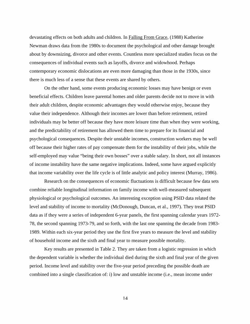
The PSID’s long-run scope and careful measurement of income enabled Duncan et al.

(1998) to investigate the importance of childhood-stage-specific poverty for completed

schooling. Their sample consisted of 1,323 children born between 1967 and 1973, who were

observed in PSID families for the entire period between birth and age 20-25 and constitute a

representative sample of children in these birth cohorts. To allow for the differential impact of

income by childhood stage, they related years of children’s completed schooling to measures of

family income averaged over the first, second and third five-year segments of the children’s lives

(Table 5).21

[INSERT TABLE 5 HERE]

Taken as a whole, the results show that the timing of economic deprivation matters a

great deal for the schooling outcomes, with income early in life by far the most important. The

coefficients reported in Table 5 suggest that, controlling for income in other stages and other

family conditions, children in families with birth-to-age-five incomes between $15,000 and

$25,000 average two-thirds of a year more schooling – about one-third of a standard deviation –

relative to children in families with less than $15,000 income. In contrast, income from middle

childhood and adolescence failed to predict strongly to the schooling outcomes.22

21 The regression models also control for mother’s schooling, family structure, race, gender, and the ageof the mother at the birth of the child, total number of siblings, whether ever lived in South, number ofgeographic moves and number of years mother worked for 1000+ hours. Parental income is inflated to1993 price levels.

22 As shown in Table 5, Duncan et al. (1998) did find that high parental income during adolescence had astrong positive effect on completed schooling. Additional analyses produced the unsurprising result thathaving affluent parents as a teenager increases your chances of attending college.

25

In short, economic deprivation occurring early in childhood appears to have the most

pronounced and longest-lasting effects on children’s achievement. The lens of early childhood as

the critical period with respect to economic deprivation leads to some important policy

implications (Duncan and Brooks-Gunn, 1998). For example, the five-year time limits in the

1996 welfare reform legislation are not as worrisome as sanctions, since few families hitting

five-year limits will contain young children living with them but many families sanctioned off

TANF programs will. More generally, income support programs are much less expensive if

directed at families with young children rather than children of any age.

Are there undiscovered dynamics in noneconomic phenomena?

John Modell encourages me to speculate about whether an annual or even more frequent

panel study version of the General Social Survey, the National Election Study, or some of the

landmark long-term developmental studies would revolutionize our thinking about the dynamic

nature of attitudes or developmental pathways as the PSID has done with respect to poverty,

welfare use, labor supply and other economic phenomena. Of course there are many examples of

two- or three-wave panels involving noneconomic phenomena, some of which take their

measurements at long intervals. None, to my knowledge, interviews frequently enough to

provide the kind of motion picture that the PSID produces about its economic and demographic

core.

Cast in event-history terms, such studies would enable us to ask whether attitudes,

psychological states or behaviors follow predictable “spell” patterns. Are changes gradual or

sudden, perhaps in response to important individual or environmental events? How often and for

what kinds of people do changes in attitudes and behaviors prove transitory?

Such data would also enable us to address whether our conceptions of constancy and

change should be supplemented with a focus on instability. Is instability in domains other than

income a predictor of important health and other significant outcomes?

Nesselroade and Featherman (1997) argue that developmentalists’ preoccupation with

stability has led them to ignore powerful theoretical and empirical reasons for needing to

understand the nature and determinants of intra-individual change. They point out that the life-

26

span perspective’s focus on changes in individuals’ capacity and performance as well as

adaptations to changing environments should lead us to view variability as the norm and stability

as the exception.

And yet most developmental research focuses on either relatively stable differences

between individuals, or on changes in a given individual that occur between measurement points

months or even years apart (Alwin, 1994, Costa and McCrae, 1980), but almost never on

duration or stability. Lacking panel data, we are tempted to infer life-cycle change by comparing

individuals of different ages from cross-sectional data, which is precisely the mistake made in

life-cycle studies of economic well-being.

Even with panel data, however, we refuse to take instability and short spells seriously.

We compute test-retest correlations from panel data gathered over short intervals to measure

reliability rather than instability, which reflects our belief that most of our constructs are stable

over at least short periods of time. Measures that exhibit instability are discarded by this process,

rather than seen as potentially valuable examples of short-duration or unstable phenomena. Few

developmental or attitudinal analyses are cast as event-histories. 23 Think of how much less we

would know about subatomic processes if we required particles to live for at least one second!

Analogously, consider the fact that we would miss at least half of the action in understanding

welfare receipt if we required spells to be at least three years in duration. What are we missing if

we don’t have a PSID-type motion picture of developmental processes?

Some intriguing evidence suggests that turbulence matters in other-than-economic

domains. Eizenman et al. (1997) gathered measures of locus of control and perceived

competence over 25 consecutive weeks from a sample of elderly residents of a Pennsylvania

retirement community. They derive measures of both the level and the stability of these two

constructs and then relate both dimensions to the mortality status of their sample five years after

23 The 1997 meetings of the Society for Research on Child Development featured a wonderful lecture byMark Applebaum, who nominated “cutting edge” methodologies for inclusion in developmentalists’methodological toolkits. I was shocked when he included event-history methods, since I had presumedthat they were widely known and used. But then I reflected on my limited reading of the developmentalliterature and realized that there were virtually no examples in which developmental processes and stageswere analyzed with duration-based methods.

27

their final measurement. As McDonough et al., (1997) found in the case of income instability,

they discover that the instability of locus of control and perceived competence is highly

predictive of subsequent mortality. In fact, instability in these dimensions was considerably more

predictive of mortality than was level.

The more general answer to the question of whether motion-picture panel studies of

other-than-economic phenomena would revolutionize conceptions of these phenomena is, of

course, “we do not know.” Nor are we likely to find out soon, since duration and turbulence are

understudied dimensions of the constructs that interest us. It makes sense to begin to investigate

these issues with small, well-focused Eizenman et al.-type studies before thinking about more

expensive large-scale studies.

ME, WITHOUT THE PSID

In 1994 I left Michigan and the PSID and joined the faculties of the Human Development

and Social Policy (HDSP) program and Institute for Policy Research at Northwestern University.

Although my attachment to both the PSID and the Survey Research Center caused me to agonize

over the decision, it is now clear that the change was a good one.

My interests in interdisciplinary work involving human development, economics and

social policy meshed perfectly with the structure and philosophy of HDSP. Fulfilling an ambition

formed as a Grinnell undergraduate, I traded administrative duties running the PSID for the

rewards of teaching and mentoring the remarkably motivated, capable and mature HDSP

graduate students. And the Institute for Policy Research has provided a fertile environment for

sustaining my research program. I surprised myself with the extent of my comfort with only an

interdisciplinary affiliation and pushing for neither a joint nor even courtesy appointment in

Northwestern’s prestigious economics department.

My experiences have reinforced my excitement over the synergistic possibilities of

incorporating economic and policy insights into studies of human development. At the risk of

oversimplication, developmentalists are strong on theory and measurement but weak in thinking

critically about the fact that peoples’ contexts are, in large part, chosen (endogeneous) and in

thinking systematically about the policy implications of their research.

28

The endogeneity problem is especially important. Does a positive association between a

high-quality child care setting and a child’s school subsequent readiness tell us that child care

quality promotes school readiness or that school readiness is caused by the same, often-

unmeasured parental characteristics that led to the choice of high-quality child care? The

psychologist’s and sociologist’s first instinct is to assume the former; the economist’s the latter.

If most resilient children are found to have had an adult mentor, does this indicate that adult

mentors would help unresilient children or merely that a manifestation of resilience is the

seeking out of mentors? The policy implications depend fundamentally on the answers to these

questions.

Economists are strong on the policy side, ask some interesting theoretical questions and

have developed a useful toolkit of techniques and approaches for the endogeneity problem. The

gulf in vocabulary, methods and instinct is wide, but by no means insurmountable.

Some of my research still uses data from the PSID. Intriguing in this work are results

indicating that some of the social-psychological measures included in the PSID’s early waves are

much more predictive of long-run and intergenerational success than of short-run outcomes.

Early analyses of the short-run (i.e., five-year) effects on labor-market earnings of measures such

as personal control and achievement motivation failed to show robust and important connections

(Duncan and Morgan, 1981; Augustyniak, et al., 1985). However, when Rachel Dunifon and I

(1998) related levels of labor-market success in the early 1990s to the early-wave measures of

personal control and components of achievement motivation, we found linkages that are much

more powerful. In fact, the collection of 25-year-old social-psychological measures accounted

for as much of the variation in current earnings as did completed schooling.

Moreover, recent work on the intergenerational effects of these early-wave measures

(Yeung, Duncan and Hill, forthcoming) shows the power for boys’ future success of some

behavioral traits of their fathers. In particular, having a risk-averse father (i.e., reports fastening

his seat belt, having car or medical insurance, etc.) is a highly predictive of the son’s completed

schooling and early-career attainments. Perhaps having a father who dampens rather than

reinforces the excesses of youth is beneficial for boys. At any rate, these two sets of long-run

results suggest the value for attainment research of taking a very long view.

29

For the most part, though, I have also surprised myself at the speed with which other data

have replaced the PSID in my research. My work with the MacArthur Middle Childhood

Network has led John Modell, post-doctoral fellow Lori Kowaleski-Jones and me to apply some

of the methods developed for understanding the dynamics of income trajectories to children’s

achievement and behavior-problem trajectories.24 Every-other-year data on behavior problems

and achievement from the National Longitudinal Surveys of Youth Child Survey display

developmental trajectories that bounce around almost as much as does family income.

Surprisingly, the seemingly chaotic developmental trajectories share many of the characteristics

of income trajectories: heterogeneous levels and slopes and a substantial random component. In

the case of the developmental trajectories, there is a tendency for girls to return more slowly than

boys to their individual “permanent” trajectories if thrown “off course” (Kowaleski-Jones and

Duncan, forthcoming).

More ambitious are my projects involving randomized experiments, which offer much

greater power than population surveys for addressing endogeneity problems. Such problems

became painfully clear as Jeanne Brooks-Gunn, other members of the SSRC committee and I

worked with PSID and other data to understand how neighborhood conditions affected children’s

development. Families are not assigned randomly to their neighborhoods, raising the question of

whether the apparent neighborhood “effects” emerging from our regressions merely reflected

unmeasured family factors that affected both choice of neighborhood and child well-being

(Duncan and Raudenbush, 1999).

Few developmental studies of contextual effects recognize, much less solve, the problem

of bias caused by unmeasured selection factors. Jens Ludwig and I tackle these problems by

taking advantage of Ludwig’s involvement with the Department of Housing and Urban

Development’s Moving to Opportunity (MTO) experiment. In MTO, poor families from public

housing projects in five of our nation’s largest cities are offered a chance to enter a program that

facilitates moves to low-poverty neighborhoods. Since families are randomly assigned to one of

three “treatments,” one of which provides no additional help at all, the problem of omitted-

24 John Modell’s proper insistence on an historical element to our research has led him to conduct aparallel analysis of life-course patterns of communion attendance in 19th century Sweden.

30

variable bias is eliminated. Early results indicate large beneficial effects of moving to lower-

poverty neighborhoods on the criminal behavior (for violent but not property crimes) of

adolescent boys in these families (Ludwig, Duncan and Hirschfield, 1998).

A second project that has added a developmental component to a randomized anti-

poverty experiment is called New Hope. Beginning in the early 1990s, New Hope offered low-

income families in two poor areas of Milwaukee the chance of a “contingent social contract” –

work 30 hours per week and receive a generous set of supports (a wage subsidy, childcare, health

insurance and, if needed, a temporary community service job). Interested families were randomly

assigned to a group eligible to receive these supports and a control group that was eligible to

receive only the supports available to all low-income families from the city and state.

Understanding how this program affects family functioning and child development is the

goal of our eclectic subgroup (Aletha Huston, Robert Granger, Vonnie McLoyd and Tom

Weisner) of MacArthur Network members. Our methods include surveys two and five years into

the program as well as qualitative interviews with a randomly-chosen subset of both program and

control families.

Since Milwaukee is only a 90-minute drive from Evanston, we have been able to involve

four HDSP graduate students in both the qualitative and quantitative work, three of whom are

using both methods simultaneously. Working with these talented students and fellow Network

members to make sense out of results from both ethnographic and survey data from a

randomized experiment is my working definition of a research Nirvana. Although this work is

still in progress, it is already clear that it is the interaction between the qualitative and

quantitative methods that has proved most interesting and rewarding. We simply would not have

been able to nail down the experimental-effects story without the insights gathered by the

students over the course of their many hours of conversations in the living rooms of New Hope

families.

With data from many other welfare experiments and new developmental surveys coming

on line in the next few years, we will have the opportunity to learn much more about the nature

and policy implications of welfare reforms for family process and children’s development. Two

ambitious child development supplements, in 1997 and planned for 2001, will keep the PSID in

31

the forefront of this work. I do not yet know whether I will become one of the analysts of these

new sets of PSID data. Whatever my future may bring, the PSID’s marks on my own

development will remain indelible.

32

Ref er ences

Alwin, D.F. 1994. “Aging, Personality and Social Change: The Stability of IndividualDifferences Over the Adult Life Span.” In Life-Span Development and Behavior,edited by D.L. Featherman, R.M. Lerner, and M. Perlmutter. Hillsdale, NJ:Lawrence Erlbaum Associates.

Augustyniak, Sue, Greg J. Duncan and Jeffrey Liker. 1985. “Panel Data and Models ofChange: A Comparison of First Difference and Conventional Two-Wave Models.”Social Science Research 14: 80-101.

Bane, M. J. and David T. Ellwood. 1986. “Slipping In and Out of Poverty: TheDynamics of Spells.” Journal of Human Resources 21: 1-23.

Bane, M. J. and David T. Ellwood. 1994. Welfare Realities. Cambridge, MA: HarvardUniversity Press.

Brooks-Gunn, J. and Greg J. Duncan. 1997. "The Effects of Poverty on Children.” TheFuture of Children 7(2): 55-71.

Burkhauser, R. and Greg J. Duncan. 1994. Sharing prosperity across the age distribution:A comparison of the United States and Germany in the 1980s. The Gerontologist34:150-160.

Children’s Defense Fund. 1994. Wasting America’s Future. Boston: Beacon Press.

Costa, P.T. and R.R. McCrae. 1980. “Still Stable After All These Years: Personality asa Key to Some Issues in Adulthood and Old Age” in Life-Span Development andBehavior, edited by P. Baltes and O.C. Brim. New York: Academic Press.

Dunifon, Rachel and Greg J. Duncan. 1998. “Long-Run Effects of Motivation on LaborMarket Success.” Social Psychology Quarterly 61(1): 33-48.

Duncan, Greg J. 1988. "The Volatility of Family Income Over the Life Course." InLife-Span Development and Behavior, edited by P. Baltes, D. Featherman, andRichard M. Lerner. Hillsdale, NJ: Lawrence Erlbaum Associates.

Duncan, Greg J., and Jeanne Brooks-Gunn (eds.) 1997. The Consequences of GrowingUp Poor. New York: Russell Sage.

Duncan, Greg J., Bjorn Gustafsson, Richard Hauser, Guenther Schmaus, StephenJenkins, Hans Messinger, Ruud Muffels, Brian Nolan, Jean-Claude Ray, andWolfgang Voges. 1995. "Poverty and Social-Assistance Dynamics in the UnitedStates, Canada and Western Europe" in Poverty, Inequality and the Future of Social

33

Policy: Western States in the New World Order, edited by Katherine McFate, RogerLawson and William J. Wilson. New York: Russell Sage.

Duncan, Greg J., Richard Coe, Mary Corcoran, Martha Hill, Saul Hoffman, and James N.Morgan. 1984. Years of Poverty, Years of Plenty: The Changing EconomicFortunes of American Workers and Families. Ann Arbor: Institute for SocialResearch.

Duncan, Greg J. and James N. Morgan. 1981. "Sense of Efficacy and Changes inEconomic Status--A Replication." Journal of Human Resources 16(4): 649-657.

Duncan, Greg J. and Stephen Raudenbush. 1999. “Assessing the Effects of Context inStudies of Child and Youth Development.” Educational Psychologist 34(1): 29-41.

Duncan, Greg J., Wei-Jun Yeung, Jeanne Brooks-Gunn and Judith Smith. 1998. "HowMuch Does Childhood Poverty Affect the Life Chances of Children?" AmericanSociological Review 63(3): 406-423.

Eizenman, D . R., J .R. N es selroade, D .L. F eatherman, and J.W. Rowe. 1997. “I ntra- I ndividual Variability in Perceived Contr ol: The M acA rthur S ucces s ful A gingS tudies.” Psychology and Aging 12: 489-502.

Elder, G. H. 1974. Children of the Great Depression. Chicago: University of ChicagoPress.

Ellwood, David. 1988. Poor Support: Poverty and the American Family. New York:Basic Books.

Fitzgerald, John, Peter Gottschalk, and Robert Moffitt. 1998. “An Analysis of SampleAttrition in Panel Data: The Michigan Panel Study of Income Dynamics.” Journalof Human Resources 33(2): 251-299.

Hill, Martha. 1992. The Panel Study of Income Dynamics. Beverly Hills: SagePublications.

Kowaleski-Jones, Lori and Greg. J. Duncan. Forthcoming. “The Structure ofAchievement and Behavior Across Middle Childhood” Child Development.

Liker, J. K., and Glen H. Elder. 1983. “Economic Hardship and Marital Relations in the1930's.” American Sociological Review 48: 343-359.

Luwig, Jens, Greg. J. Duncan, and Paul Hirschfield. 1998. “Urban Poverty and JuvenileCrime: Evidence from a Randomized Housing-Mobility Experiment.”Northwestern University/University of Chicago Joint Center for Poverty ResearchWorking Paper, November 1998, #2.

34

Mayer, Susan. 1997. What Money Can’t Buy. Cambridge, MA: Harvard UniversityPress.

McDonough, Peggy, Greg J. Duncan, David Williams, and James House. 1997. “IncomeDynamics and Adult Mortality in the U.S., 1972-1989.” American Journal ofPublic Health 87(9): 1476-1483.

Morgan, James N. et al., 1974. Five Thousand American Families--Patterns ofEconomic Progress, Vol. I. Ann Arbor: Institute for Social Research.

Murray, Charles. 1986. “According to Age: Longitudinal Profiles of AFDC Recipientsand the Poor by Age Group”. Prepared for the Working Seminar on the Family andAmerican Welfare Policy.

Newman, Katherine. 1988. Falling From Grace: The Experience of Downward Mobilityin the American Middle Class. New York: Free Press.

N es selroade, J . R. and D . L. F eatherman 1997. “Es tablis hing a Ref er ence Fr ame A gains tWhich to Char t A ge-Related Changes” in Studying Aging and Social Change:Conceptual and Methodological Issues edited by M. A . H ar dy. Newbury Park, CA:Sage Publications.

Tuma, N.B. and L.D. Groeneveld. 1979. “Dynamic Analysis of Event Histories.”American Journal of Sociology 84: 820-854.

Weitzman, Lenore. 1985. The Divorce Revolution. New York: Free Press.

Yeung, Wei-Jun J., Duncan Greg J., and Martha S. Hill. Forthcoming. "Putting FathersBack in The Picture: Parental Activities and Children's Attainment", Journal ofMarriage and Family Review

35

Tab le 1: Level and s t ab ility of income, 1969- 79 by age and s ex

A ge in 1969/S ex M ean incomelevel, in

thous ands of1985 $

P er cent withincome r is ing

r apidly

P er cent withincome f alling

r apidly

% w ith big( >50% ) dropsin income atleast once

O f those w ithdrops , % expecting

income los s

Pat

25- 54 yrs M en $43.1 35% 6% 18% 9%

Women 40.0 32 10 24 646- 55 yrs

M en 38.7 22 13 26 12Women 32.3 21 20 33 24

56- 65 yrs M en 29.5 7 38 38 34

Women 22.1 6 35 39 25

N ote: Taken f rom D uncan ( 1988) . “Rapid r ise” in size- adjus ted income is an increase gr eater than 5% per yeaadjus ted income is a decr eas e greater than 5% per year. Over an eleven-year period, an annual real growth rate of 5 percent willincrease a family's real income by over 70 percent; a negative 5 percent rate will nearly cut it in half.

36

Table 2: Odd-ratios of mortality for individuals aged 45-64 years, by income leveland stability, 1972 through 1989

Five-year mean incomelevel and stability

Odds ratio 95% confidence interval

Income <$20,000 and 1+income drops 3.7*

2.4-5.7

Income <$20,000 and noincome drops 3.4*

2.2-5.1

Income $20-$70,000 and 1+drops 3.2*

1.9-5.5

Income $20-$70,000 and nodrops 1.5*

1.0-2.0

Income >$70,000 and 1+drops 1.4

0.7-2.6

Income >$70,000 and nodrops 1.00 (reference group)

-

Note: Taken from McDonough et al. (1997), Table 3. “Income drop” is defined as asituation in which size-adjusted family income fell by 50% or more in consecutive years.

“*” indicates that the coefficient is at least twice its standard error. Odds ratios areadjusted for age, sex, race, family size and period.

Table 3: Distribution of lengths of spells of poverty and AFDC, for individuals firstbeginning spells of poverty and AFDC

Poverty, for nonelderly personsbeginning a poverty spell

Aid to Families With DependentChildren, for women first beginningan AFDC spell

1-2 years 60% 36%

3-7 26 35

8+ 14 29

TOTAL 100% 100%

Source: Poverty data taken from Bane and Ellwood (1986, Table 2); AFDC data takenfrom Bane and Ellwood (1994, Table 2.3)

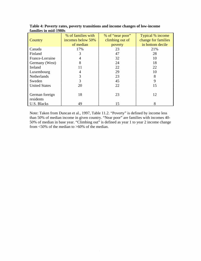
37

Table 4: Poverty rates, poverty transitions and income changes of low-incomefamilies in mid-1980s

Country% of families with

incomes below 50%of median

% of “near poor”climbing out of

poverty

Typical % incomechange for families

in bottom decileCanada 17% 23 21%Finland 3 47 28France-Lorraine 4 32 10Germany (West) 8 24 18Ireland 11 22 22Luxembourg 4 29 10Netherlands 3 23 8Sweden 3 45 9United States 20 22 15

German foreignresidents

18 23 12

U.S. Blacks 49 15 8

Note: Taken from Duncan et al., 1997, Table 11.2. “Poverty” is defined by income lessthan 50% of median income in given country. “Near poor” are families with incomes 40-50% of median in base year. “Climbing out” is defined as year 1 to year 2 income changefrom <50% of the median to >60% of the median.

38

Table 5: Effects of stage-specific parental income on completed schooling and high-school graduation rates

Income averaged over:Years of completed schooling

AGE 0-5Below $15,000 .00 (reference group)

$15,000-$24,999 .66*$25,000-$34,999 .73*$35,000-$49,999 .78*

$50,000 and above 1.41*

AGE 6-10Below $15,000 .00 (reference group)

$15,000-$24,999 .16$25,000-$34,999 .24$35,000-$49,999 .44

$50,000 and above .33

AGE 11-15Below $15,000 .00 (reference group)

$15,000-$24,999 .34$25,000-$34,999 .41$35,000-$49,999 .36

$50,000 and above 1.08*

Note: Based on Duncan et al., (1998), Table 3. “*” indicates that the coefficient is at leasttwice its standard error. All regressions include controls for mother’s schooling, familystructure, race, gender, and the age of the mother at the birth of the child, total number ofsiblings, whether ever lived in South, number of geographic moves and number of yearsmother worked for 1000+ hours. Parental income is inflated to 1993 price levels.

Notes on the 'Income Plus' Files

1994-1997 Family Income and Components Files

Yong-Seong Kim, Tecla Loup, Joseph Lupton, and Frank P. Stafford

March 11, 1999

FIRST REVISION April 2000 SECOND REVISION December 20, 2000

I. Introduction and Overview These files contain data and documentation for the Panel Study of Income Dynamics' 1994, 1995, 1996, and 1997 Total Family Income and its components. These files also include the state of residence for each of these four waves as defined by the PSID and FIPS state codes. Originally, these files included the three-digit 1970 Census occupation and industry codes for head's and wife's/"wife's" current or most recent main jobs, for the 1996 wave only. In April 2000, these codes were added for the 1994 and 1995 waves as well. Coding for 1997 has not been completed as of this writing. We expect to post 1999 occupations with the 1999 files. Also in April 2000, both USDA and Census Needs Standards were added for all four waves. This file provides basic information about these 1994-1997 income files. We recommend that you carefully review the following material before proceeding with any work using the data files. Over the last two years the PSID Staff have taken steps to develop new processing software to be applied to the (Computer Assisted Telephone Interviewing) CATI output for family income and its components. For those familiar with the complex PSID income sequences for head, wife and other family unit members, this will be recognized as an ambitious project. An initial version of the Income Processing Software (IPS) was completed in the early fall of 1997 (CATIINC 1.0), and a modified version was completed (CATIINC 2.0) in the late summer of 1998. A further revised version was developed (CATINC 3.0) in the summer of 2000. This CATI 3.0 is more sophisticated in identifying anomalous cases. For example, the newest IPS version incorporates information from prior waves (and, if available, subsequent waves) to identify potentially problematic cases of data entry error. 1. Early work with the income data from the PSID Income Plus files showed that the post-CATI data, 1993-1997, have a higher variance and that this seems to be concentrated in about 50 cases per year (out of 7,000 – 8,500 cases). Having extensively reworked our Income Processing Software (IPS) in the spring and summer of 2000 to create CATINC 3.0, we have recently applied it and edited additional cases. This new version of IPS is meant to work in tandem with our new editing system—more on this below. The IPS calculates income and its components in a straightforward way if all elements are there and there are no item non-responses or other anomalies in the underlying components. For the cases with unusual features one can calculate values from partial information. But this has limits. Also, simple keystroke errors in CATI can give rise to valid, but extreme values. To identify large, artificial changes in income

components—such as labor income—the program flags ‘large changes,’ particularly if not accompanied by a change in occupation and/or industry. These flagged cases are looked up to assess the larger context of the record including possible interviewer text fields of notes taken during the interview. If a better judgment edit can be made, a value is assigned. If not, a simple imputation may be used. Cases so modified are recorded as modified for the user. 2. The IPS output is intended to be then edited within an editing system. This system is described more fully below. In the interim we have effected a simpler (but time intensive) version of that system by creating Excel files of the input that goes into an income calculation and using that information for editing. This has lead to what we regard as very good income data for labor income and total family income. There are still some very minor improvements to the income files, 1994-1997 and 1999 which will be carried out for final archiving in our new edit system. How does our pre-archived income data look? An overview of Total Family Income, 1968-1999 is provided in Figure 1 where we have carried out the application of the extensively revised IPS to process income from its detailed components and have carried out numerous checks for both cross-sectional and cross-wave outliers to identify potentially anomalous cases. IPS has also treated the SEO sample (see the PSID website under 'Overview' and then ‘Sample’) differently. In the case of imputations for missing data it has developed within-SEO sample conditional values to avoid imparting a systematic upward bias for those cases. Across all four waves, 1994-1997, there were about 800 cases deemed to need some case-by-case checking. (Sort of like challenges in the NFL.) Overall, about 200 cases were changed, 1994-1997, with more of the changes in 1994, and fewer per year going forward to 1997. These changes are mostly designed to improve the data quality for panel analysis, but show up as a modest reduction in the cross-sectional variance of income.

Figure 1

total family income

0.0

10000.0

20000.0

30000.0

40000.0

50000.0

60000.0

70000.0

y_

68

y_

70

y_

72

y_

74

y_

76

y_

78

y_

80

y_

82

y_

84

y_

86

y_

88

y_

90

y_

92

y_

94

y_

96

PSID faminc

$ in

19

97

mean

std

From Figure 1 there are two data ‘eras’: one 1968 to 1979 and then post 1980. Throughout there is a steady upward rise in (family weighted) total family income in 1997 CPI-U dollars, from $35,628 in 1967 (1968 survey year) to $48,394 in 1996 (1997 survey year). The standard deviation of family income appears smooth through time up to 1979 and then from 1980 forward is higher and more variable per year. The explanation for this change is that prior to 1979 the topcode value of income was $99,999. In 1980 it was increased to $999,999 and in 1981 it was increased to $9,999,999. The reasons for topcoding at $99,999 prior to 1980 appear to have been limits on logical record length in the early file structures of the PSID and a concern that top values may be dominated by reporting error. The current philosophy is to provide as many digits as needed to portray the full range of income, to check to be sure that insofar as possible these high values are valid and not keystroke errors, and allow the analyst to deal with issues of robust estimation. For the period 1968 to 1993, income was also bottom coded at $1. This means that a few families with negative total family income, arising typically from a business or farm loss were set to $1. For 1994-1997 the Income Plus files allow a negative total family income. For the purpose of constructing Figure 1, the negative and 0 values for 1994 to 1997 were set to $1 to maintain comparability with pre-1994 bottom coding. One purpose for bottom coding appears to be simplicity in calculation income-to-needs ratios, a key goal in the study, particularly in its early years when the central focus was the study of poverty and income needs of the U.S. population. The data in Figure 1 show a higher standard deviation after the top coding change in 1979-1980. This is not surprising, and Figure 2 shows the total family income series 1968-1997 if the

topcoding at $99,999 had been extended throughout. In that case the standard deviation is always below the mean and exhibits relatively little year-to-year variation throughout. The standard deviation in total family income in the Income Plus files for 1994-1997 seems quite in line with the long term pattern.

Figure 2

total family income (top adj)

0

5000

10000

15000

20000

25000

30000

35000

40000

45000

50000

y_

68

y_

70

y_

72

y_

74

y_

76

y_

78

y_

80

y_

82

y_

84

y_

86

y_

88

y_

90

y_

92

y_

94

y_

96

PSID faminc

19

97

$ mean

std

A concern is that even with careful data processing with IPS and individual case editing, the CATI based income could be dramatically different from paper and pencil and individual editing prior to 1993. One simple check is suggested by referring back to Figure 1. Throughout the period when topcoding was extended to $9,999,999 there are much larger year-to-year variations in the cross section standard deviation of total family income. Further there are three post-1979 ‘episodes’ of notably higher standard deviation values: the early 1980’s recession and recovery of 1981-1983, the late 1980’s expansion of 1987-1989, and the post-Gulf War expansion of 1994-1996. There does not appear to be a pure CATI effect, since 1993 differs from 1994-1996 and 1997 is about in the same range as 1993. Within the CATI years, then 1993 and 1997 are ‘low’ in terms of post-1980 values for the standard deviation, and 1994-1996 are ‘high’ in these same terms. Despite the apparent similarity in the overall cross sectional income measures (after an enormous effort to maintain comparability in the face of extensive technical changes) the output from each year since the 1992 survey has had its own set of special input problems, owing to successive changes and improvements in the CATI software. In 1993 there was a migration from the

traditional paper questionnaire to an initial CATI application. This has the potential to have created a seam problem in the income data, given the complex structure of the PSID question sequences designed to measure income at the detailed component level by person within the family. In processing the 1993 family income there was a need to create an initial version of our software system which paralleled the pre-1993 system of software and editing of paper questionnaires. This is necessarily different in numerous details from the prior system, again creating a potential seam in the income data. For 1994 there were additional changes to CATI and the 1994 data in these files, as noted above, have been processed by the CATIINC 3.0 software. From 1995-1997 the CATI system had been stabilized and we are applying the same software for these files, so these 1994/5-1997 family income data should be quite consistent with one another. The issue for researchers to consider then is a potential double seam created by a shift to CATI and a concomitant change in the processing software in 1993 and 1994. It is our judgment that the seam problem created by CATI collection itself was quite minor. To illustrate, a 1994 study of recording errors in 200 cases assigned to CATI and 200 cases in paper and pencil shows similar rates of recording errors. The potentially far more important source of non-comparability is in the processing system – the system which takes partial and otherwise anomalous cases and reaches an estimate or imputation for a ‘final value’. Taking the processed 1994-1997 output from CATINC 3.0, cases were reviewed and adjusted, if that was deemed best. For example, by misreporting the `per' variable, a respondent could have $75,000 `per year' miscoded as $75,000 `per week'. A file of these corrections was kept, by year, so that those wishing to apply alternative editing judgments can do so. In the paragraphs below we provide the user with a selection of the extreme cases which we `hand edited' after having employed our program to compute family income and its components. We have recently (September - December of 2000) reviewed the labor income of head and wife and have `hand edited’ an additional set of the cases with high values of transfer income. The components of transfer income are very diverse. This has made it difficult to carefully evaluate outliers without a case by case review of the interview and interviewer thumbnail comments—plus information on the family from prior and subsequent years. Analysts are urged to exclude or otherwise allow for cases in which the value of transfer income is above the top 99.5 percentile point. Also, analysts may want to either exclude or allow for these cases n the analysis of income totals which have such extreme values in them (i.e. total family income, taxable income of the head and wife) or to assign the transfer income part of these family aggregates to zero or the median of transfer income. ILLUSTRATIVE POST SOFTWARE CASE `HAND' OR JUDGMENTAL EDITING: 1997 ID=02314 had Social Security income of $1,214,952. The head reported $15,000 a year, and the wife reported $99,996 per month! Checking the marginal notes, we read that the COMBINED head and wife Social Security income was $15,000 for the year; the interviewer entered this amount for the wife intending to alert us to the fact that head and wife couldn't separate their respective amounts. (It worked, but this is not what she would have been advised

to do—yet she made this judgment on the spot to continue the interview.) We recoded the amount to $15,000. 1997 ID=01368 had head and wife transfer income of $347,041. This was due to an `other retirement pension' amount of $308,712. From other evidence, the amount seemed unlikely for this family. We checked back to 1996, where the same item was reported as $3,087. It appears that the 1997 other pension reported amount is missing a decimal and should be $3087.12, or rounded to $3087. In addition, this family reported $38,329 from "anything else" (miscellaneous transfers), with no marginal note explaining the source. Checking the 1996 and 1995 interviews, no similar amount had been reported. We judged that the $38,329 is a lump sum payment of some kind, probably health insurance reimbursements—the head has been ill, in and out of nursing homes and hospitals. So their total transfers were entered as $3087 for 1997. 1997 ID=05135 had other family unit member (OFUM) transfer income of $221,132. Two OFUMs, a son and a girlfriend, were in this family unit (FU). The son reported $511/month of Supplemental Security Income (SSI), received all year, for a total of $6132. The girlfriend reported "anything else" of $10,000/week received in Jan, Mar, June, August, and November. Aside from the fact that it appears she means $10,000 per year, this money is from student loans and should be entirely removed from income. We never consider loans as income, period. So total OFUM transfers for this case=$6,132. 1996 ID=00427 had head and wife transfer income of $238,446. Here are all the non-labor components: the `wife' reported $500/yr dividends—which seems ok, $2000/yr interest—which seems ok, but $18,000 per WEEK help from relatives! This is not ok! Checking back to 1995, she reported $20,000 per year for the same thing. So the `per' time unit was judged to be `per year' rather than `per week'. In addition, head reported $18,000 per year in help from non-relatives. The marginal notes make it clear that this is double-counted with the `wife's'. So their total transfers were judged to be $20,500 per year. Cases of this sort were quite rare. When it is remembered that the field-based input on the part on interviewers for these files consisted of approximately 1.5 million data entries, the presence of some outlier cases is not surprising. Interviewing is a delicate art of continuing to engage a respondent who is providing a lengthy and complex interview via telephone. Some errors are inevitable, and not all will be caught in our processing and hand editing systems. Users need to keep this in mind and are advised to calculate descriptive statistics and quantiles on the groups and subgroups in their analyses. Users should also realize that in looking at individual cases, changes were made only if there were fairly obvious indications of misreporting (as illustrated above). Our approach is not nor has it ever been to second guess respondent reports or stylize the economic reality of the families in our study. The tradition in the PSID has been to set income data with negative or zero total family income values to $1. For these files of the 1994-1997 years, those with negative or zero total family income (arising, e.g., from a business loss or from living on liquidated assets) were simply left as negative or zero values. As discussed above users wishing to increase time series consistency may want to allow for this difference.

While we have listed and adjusted obvious outliers, there are two remaining data issues which analysts should recognize. There are 519 working wives who were skipped past the labor force CATI checkpoint in the income question series in the 1994 Survey. In the process of revising the Income Plus file, the income variable for those respondents was first flagged and was imputed using various methods including cross-year imputation. As a result, the 1994 cases of wife earnings that were treated by the IPS is increased relative to other years (see Section V: Income Editing Procedures). We have made numerous data checks by looking at time series of descriptive statistics for the years 1968-1997. Nonetheless, this is a new and complex system and income is itself highly dispersed. For analysts, robust estimation and descriptive techniques should be the order of the day. Finally, we note that the data used in this paper are all in 1997 dollars (CPI-U, 1982-1984 = 100). (The data in the released files are *not* in 1997 dollars, rather they are in actual amounts). The relevant CPI-U values are: 1997: 160.5 1996: 156.9 1995: 152.4 1994: 148.2 1993: 144.5 1992: 140.3 1991: 136.2 The conversion factors which were applied to the data by (calendar) year data were: 1997: 160.5/156.9 = 1.02295 1996: 160.5/152.4 = 1.05315 1995: 160.5/148.2 = 1.08300 1994: 160.5/144.5 = 1.10727 For those working with data from 1991-1993 to study time series patterns the conversion factors would be: 1993: 160.5/140.3 = 1.14398 1992: 160.5/136.2 = 1.17841 There was a study comparing the PSID and CPS, 1969-1991, by Greg Duncan, Timothy Smeeding and Willard Rodgers (Household Income Dynamics in the 1970's and 1980's, working paper, April 24, 1995), based on families headed by a 25-54 year old. The study showed that, particularly for the Gulf War Recession year, 1991, the PSID and CPS do line up relative to their values as of 1969. However, in the mid to late 1980's the PSID (with 1969 as the reference year) was showing substantially lower income at the lower (20 and lower) percentile points. One interpretation is that while the PSID gets a more complete income picture (more components and

detail and therefore less underreporting), in more recent years we also get a better response from people with low income and assets. This has come up in the wealth area where, in contrast to evidence from some other studies, we show that African Americans are less likely to have a bank account in the 1990's compared to the 1980's (see Erik Hurst, Ming Ching Luoh and Frank Stafford, "Wealth Dynamics of American Families, 1984-1994," Brookings Papers on Economic Activity," (1998:I), p. 296-301). These low income and low asset ownership respondents, one can hypothesize, actually report how low their income and assets are in the PSID. In summary, there are several points to bear in mind in CPS/PSID household/family income comparisons. 1. 1991 was a special (vintage) year in terms of CPS/ PSID alignment. 2. Both studies have potentially significant data seam problems in the 1990's. The post 1992 survey year CATI and processing of CATI issues for the PSID have been noted above. 3. At the median there appears to be an approximately a 0-5% PSID/CPS difference in medians between CPS and PSID for 1994(93) through 1997(96).

Table 1 Median Family Income PSID and CPS Comparison

PSID Median (1997$) CPS Median (1997$) *

Release of

March 1999 December 2000

1993 (1994 Survey) $32,749 $33,321 $34,432

1994 $34,607 $34,654 $34,807

1995 $35,070 $35,173 $35,807

1996 ** $34,985 $34,903 $35,979

* Source: http://www.census.gov/hhes/income/dinctabs.html ** In 1997, we were forced to drop 2,843 of the 3,967 families in the SEO (low income) sample because we were not successful in our efforts to secure funding for the continued data collection for this part of the core sample. The sample suspension as of 1997 and every other year interviewing changes after 1997 are discussed in our April, 1997 PSID Newsletter and our April, 1998 PSID Newsletter (viewable at this website). The 1997 family weights have been designed to apply to either the remaining pre-1997 PSID core (allowing for the 2,843 dropped SEO cases) or the 1997 core, which now includes the new sample of post-1968 immigrant (P68I) families.

II. Data There are four data files: the 1994, 1995, 1996 and 1997 Family Income and Components Files. Each file contains information about Total Family Income, which is the sum of Taxable Income of the Head and Wife plus Transfer Income of the Head and Wife plus Taxable Income of Other Family Unit Members plus Transfer Income of Other Family Unit Members plus Social Security Income. Also included are: Farm Income, Business Income, Labor Income of the Head, Labor Income of the Wife, and (for 1994) whether the labor income of the wife was assigned by imputation (as the

product of 1994 Survey Year hours times 1993 Survey Year wage rate). The state of residence, as defined by the PSID and FIPS state codes, is also included for each wave. Occupation and industry codes are added to the 1994-1996 files; these variables were not included as part of those early-release main files because they had not yet been coded when those files were released. In addition, the revised income plus file includes various components of labor income so that it helps users to identify which part of labor income might be imputed. Also variables for number of businesses owned by the family, head, and wife were generated as a by-product of the IPS. Finally, not only the total business income but also the disaggregation of labor and assets parts of the business income for Head and Wife/"Wife" are generated. Finally, both USDA and Census needs standards have been added for all four years. Note that a very few cases have missing data in these variables (1 case in 1994, 3 in 1995, 6 in 1996, and 1 in 1997). The early release family data files, which match the Income Plus files, included some family records that will not appear on the archive releases of the family files. (Cases can be invalidated for various reasons, e.g., a splitoff interview was found to be invalid because the splitoff had moved back home before the splitoff interview was taken.) The needs variables, however, were calculated using the cross-year individual file, which did not include individuals from those invalidated families. These 1994-1997 Family Income Files contain one record for each family interviewed in 1994-1997. For each year, the file includes a special sample of recontacted respondents (notably numerous in 1994), as part of a large methodology study. These 1994-1997 files do not include the special Latino sample. The case count of families in the 1994 Family Income File is 8659. For 1994 the case count of families that have a non-zero family panel weight (see the weights files for 1994-1996 released 9/98) was 7747. The difference is the consequence of the recontact families. They can be used for some analysis purposes, but simply have a zero family weight. Parallel differences of this sort exist for 1995 and 1996. Users wishing to apply FAMILY WEIGHTS in their analysis will need to visit the weight section of the data library (PSID Data Files, 1993-1997). (We do not place the Family weights here for the sake of controlling redundancy in our data library and website.) The 1997 weights are complicated by sample suspension and the addition of a refresher sample of post-1968 immigrants, but they are now available and can be applied to these 1997 family income variables. These 1994-1997 data may be subject to relatively minor changes once the archive-release versions of the 1994, 1995, 1996 and 1997 family files become available. The data are in raw ASCII form. Refer to the data definition statements—SAS or SPSS—for record format layout information, variable names, variable labels, and missing data codes.

Table 2 File Attributes and Variables for Data Files

File Name Records LRECL Num of Variables

FAMINC94 8,659 229 48

FAMINC95 8,570 228 48

FAMINC96 8,517 225 48

FAMINC97 6,307 215 44

III. SAS & SPSS Data Definition Statements These files contain SAS and SPSS data definition statements providing information about the variables in the data files. Two files, one of each type, SAS and SPSS, corresponding to each data file, are provided. The naming conventions are the same as for the data files, e.g., FAMINC94.SAS contains SAS statements for the 1994 Family Income data file, and FAMINC94.SPS contains SPSS statements for the 1994 Family Income data file. Similar files also exist for 1995-1997. The data definition statements provide variable names, variable labels, locations. These processed files have no `missing' data. The SAS and SPSS data definition statements are NOT intended to represent completed and full programs for the respective statistical program packages to run extracts, analysis, etc. You must provide all other SAS or SPSS statements needed to complete a program. Users wishing to migrate to other formats may use a commercial software for such purposes, such as STAT/TRANSFER.

IV. Documentation The following machine-readable documentation files are provided for the designated data files.

Table 3 File Description and Attributes for Documentation Files

Contents Filename Approximate Printed pages

Notes on the 'Income Plus' Files YPlsNote.doc 16

V. Income Editing Procedures General Editing Rules for Labor Income In a given year of PSID, the data were first screened to detect potentially problematic values for each component of the head and wife’s labor income variables. Programs were written to flag: 1) Don’t Know (DK) and Not Applicable (NA) (e.g., 9999998, 9999999) ; 2) ‘short’ or less than full field width codes (e.g. 9999, 9998); and 3) keystroke errors (e.g. 9996, 88889). The resulting numbers of such instances for the head and wife are reported in Tables 4 and 5.

Table 4 Number of flagged cases in head’s labor income

PSID FRM WG BNS OVT TIPS COM UK PRA GAD RM XTR Total

94 30 579 33 81 9 12 0 19 5 0 29 797 95 30 454 20 65 11 11 0 11 1 1 13 617 96 18 381 27 47 5 6 0 8 4 1 16 513 97 20 285 31 33 6 6 6 3 3 1 8 402

Total 98 1699 111 226 31 35 6 41 13 3 66 2329

* FRM = Farm income, WG=Wage and salaries, BNS=Bonus, OVT=Overtime, COM=commissions, UK=Unknown Jobs income, PRA=Professional practice, GAD=Market Gardening, RM=Roomers and Boarders, XTR=Extra job income.

Table 5 Number of flagged cases in wife’s wage income

PSID WG

94 732 95 160 96 156 97 145

Total 1193

Needless to say, these values must be replaced by real values so that any level of aggregation of labor income components yields meaningful amounts. To obtain an informed value, the following data elements were examined: 1) cross-sectional information such as from the employment section; 2) cross-year information for the same family; 3) the cross-sectional distribution from the current year employment section. When all these efforts failed to deliver a candidate value, interviewers' notes were read for a possible explanation. As indicated in Tables 4 and 5, the two most problematic components are "Wages and Salaries" and "Overtime". The procedures for these two components are discussed below. 1. Wages and Salaries: Wages and salaries reported in G13 and G52 should not include income from an unincorporated business. For such cases a zero amount was assigned and the amount was relocated to the business income section. There is useful contextual information for wages and salaries (G13 and G52) in the employment sections (B, C, D and E). By definition, wage and salary income must be closely related to hours of work. In the case where G13 or G52 had a potential problem, the characteristics of all jobs (excluding unincorporated business jobs) reported by the head (wife) were examined. For each job, wage and salary were calculated based on hours of work (= how many weeks work times how many hours per week) and the hourly wage rate. When the number of weeks was not reported, the month strings of the job (weeks = # of months worked times 4.33) were used as a proxy. Then, wage and salary income of each job that head had reported was aggregated. In some cases, hours of work and wage and salaries of other years were compared. In many cases, the wage rate (after CPI adjustment) and hours of work in other years provide useful information in imputing amounts. The variables from the employment sections, month strings for work history, were a central input to editing.

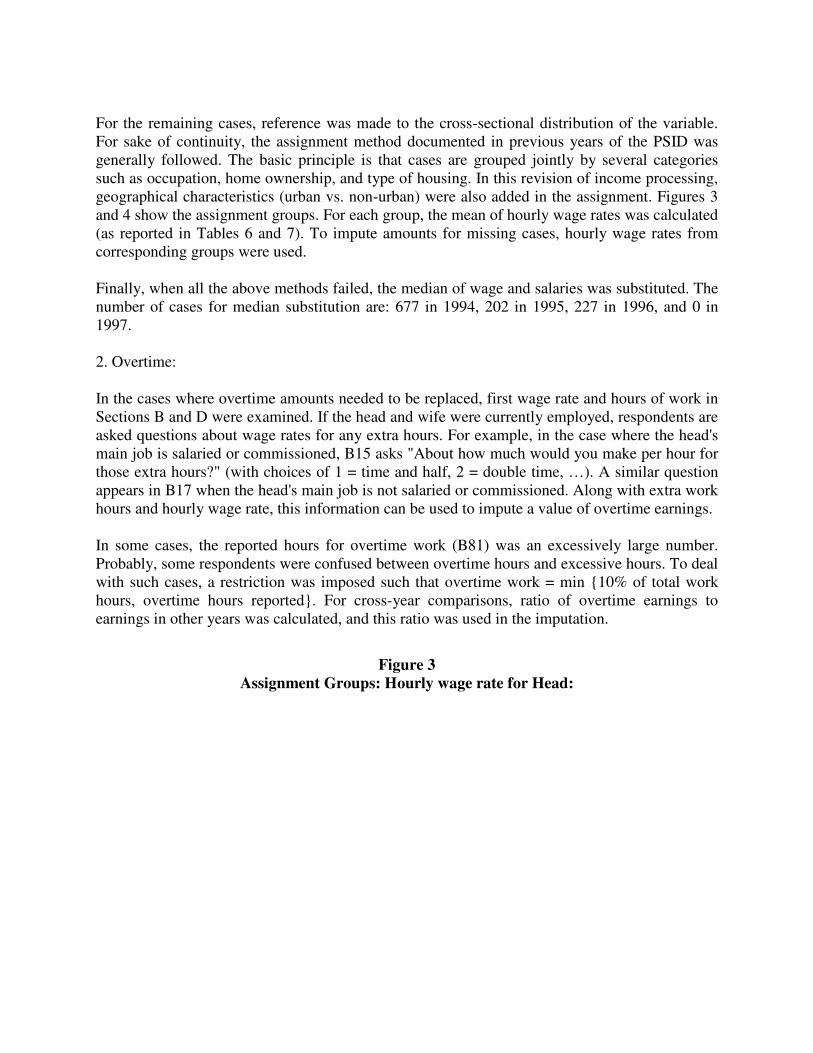
For the remaining cases, reference was made to the cross-sectional distribution of the variable. For sake of continuity, the assignment method documented in previous years of the PSID was generally followed. The basic principle is that cases are grouped jointly by several categories such as occupation, home ownership, and type of housing. In this revision of income processing, geographical characteristics (urban vs. non-urban) were also added in the assignment. Figures 3 and 4 show the assignment groups. For each group, the mean of hourly wage rates was calculated (as reported in Tables 6 and 7). To impute amounts for missing cases, hourly wage rates from corresponding groups were used. Finally, when all the above methods failed, the median of wage and salaries was substituted. The number of cases for median substitution are: 677 in 1994, 202 in 1995, 227 in 1996, and 0 in 1997. 2. Overtime: In the cases where overtime amounts needed to be replaced, first wage rate and hours of work in Sections B and D were examined. If the head and wife were currently employed, respondents are asked questions about wage rates for any extra hours. For example, in the case where the head's main job is salaried or commissioned, B15 asks "About how much would you make per hour for those extra hours?" (with choices of 1 = time and half, 2 = double time, …). A similar question appears in B17 when the head's main job is not salaried or commissioned. Along with extra work hours and hourly wage rate, this information can be used to impute a value of overtime earnings. In some cases, the reported hours for overtime work (B81) was an excessively large number. Probably, some respondents were confused between overtime hours and excessive hours. To deal with such cases, a restriction was imposed such that overtime work = min {10% of total work hours, overtime hours reported}. For cross-year comparisons, ratio of overtime earnings to earnings in other years was calculated, and this ratio was used in the imputation.

Figure 3 Assignment Groups: Hourly wage rate for Head:

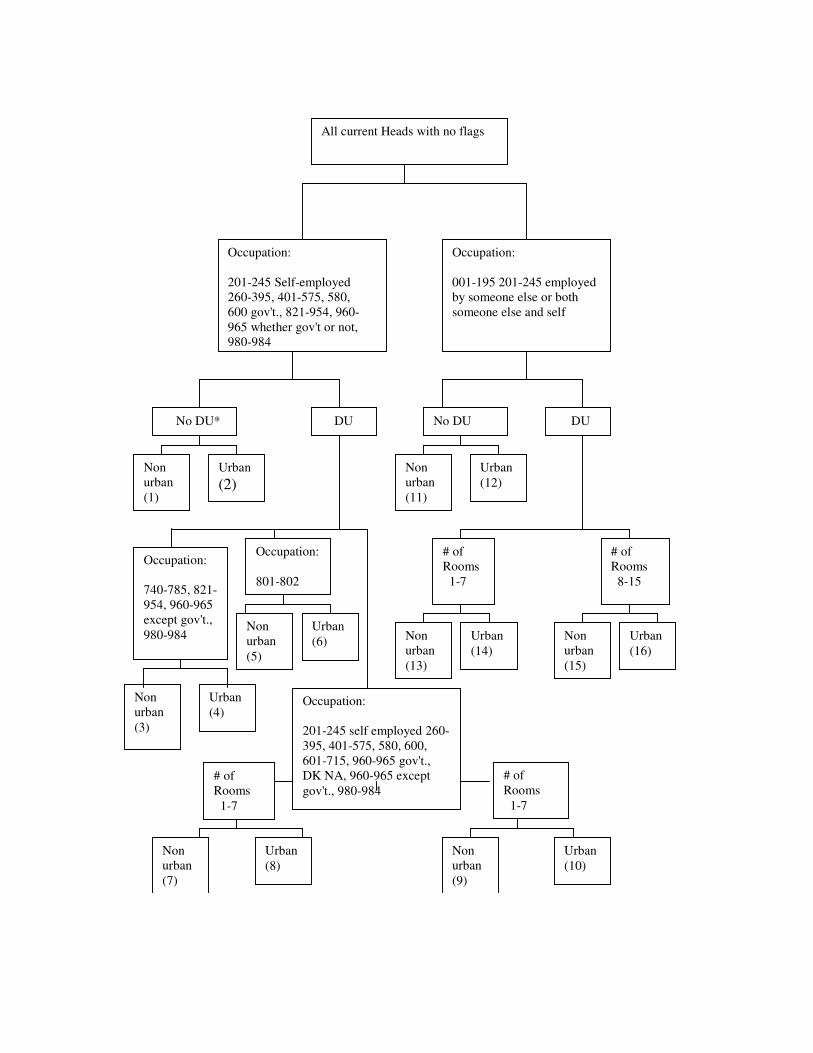
All current Heads with no flags

Occupation:

201-245 Self-employed260-395, 401-575, 580,600 gov't., 821-954, 960-965 whether gov't or not,980-984

Occupation:

001-195 201-245 employedby someone else or bothsomeone else and self

No DU* DU No DU DU

Occupation:

740-785, 821-954, 960-965except gov't.,

980-984

Occupation:

801-802

Occupation:

201-245 self employed 260-395, 401-575, 580, 600,601-715, 960-965 gov't.,DK NA, 960-965 except

gov't., 980-984

Urban

(2)Nonurban(1)

Nonurban(11)

Urban

(12)

# ofRooms 1-7

# ofRooms

1-7

# ofRooms

1-7

# ofRooms 8-15

Nonurban

(3)

Urban(4)

Nonurban

(5)

Nonurban(9)

Nonurban(7)

Nonurban(13)

Nonurban(15)

Urban

(14)

Urban

(16)

Urban(8)

Urban(10)

Urban

(6)

Table 6 Assignments for Head’s Hourly Wage Rate

PSID 94

group n Min max mean std

1 371 1.07 147.66 8.47 10.00 2 2081 1.00 162.67 9.60 9.35 3 120 1.35 166.88 9.19 15.38 4 324 1.00 113.75 10.76 10.80 7 411 1.29 100.00 11.60 8.92 8 1261 1.37 161.85 14.48 10.22 9 84 1.09 50.60 14.41 8.58

10 320 2.08 183.33 20.48 18.57 11 65 1.52 63.49 11.64 8.91 12 525 1.32 115.61 14.42 10.31 13 127 2.18 48.25 15.01 8.19 14 644 1.63 176.00 21.08 16.24 15 58 1.16 52.00 17.68 10.43 16 409 3.40 178.57 30.13 23.09

PSID 95

group n Min max mean std

1 422 1.07 94.57 9.22 7.73 2 2012 1.02 104.25 9.46 8.20 3 69 1.69 42.64 9.06 6.33 4 377 1.21 91.43 10.38 10.04 7 299 1.65 125.00 13.82 9.90 8 1324 1.03 182.55 14.38 11.80 9 94 1.25 171.22 21.92 19.66

10 338 2.64 146.94 19.29 14.52 11 111 1.69 83.56 14.76 12.28 12 463 1.02 120.45 14.70 11.26 13 165 1.04 90.91 18.97 10.64 15 96 3.85 170.07 29.44 24.35 16 345 2.92 191.49 28.40 19.88

PSID 97

group n Min max mean std

1 342 1.12 53.12 8.21 6.10 2 1612 1.00 96.34 9.85 7.95 3 114 1.07 86.09 9.56 8.66 4 229 1.11 44.80 10.94 6.16 7 377 1.01 105.47 12.47 9.27 8 955 1.15 192.46 15.60 12.42 9 85 1.44 37.12 13.95 7.36

10 305 2.50 163.27 22.94 20.12 11 79 1.50 57.33 11.17 8.23 12 471 1.56 175.53 14.47 11.47 13 125 1.46 35.42 14.40 6.10 14 556 2.05 150.00 20.84 13.42 15 46 2.61 64.00 21.55 12.31

16 384 2.25 191.49 30.55 22.18

Figure 4

Assignment Groups: Hourly Wage Rate for Wives:

Region 1 = Connecticut, Maine, Massachusetts, New Hampshire, New Jersey, New York, Pennsylvania, Rhode Island, Vermont

All current Wives with no flags

Occupation:

601-715, 740- 785, 801-802, 821-954, ,960-965except gov't, 980-984

Occupation:

201-245 Self-employed260-395, 401-575, 580,600, 960-965 gov't

Occupation:

001-195, 201-245 employedby someone else or bothsomeone else and self

Nonurban(1)

Nonurban(3)

Nonurban(5)

# ofRooms 1-7

# ofRooms 8-15

Urban(2)

Urban(4)

Urban(6)

Region 1 Region 2-4,6

Nonurban(7)

Urban(8)

Nonurban(9)

Urban(10)

Region 2 = Illinois, Indiana, Iowa, Kansas, Michigan, Minnesota, Missouri, Nebraska, North Dakota, Ohio, South Dakota, Wisconsin Region 3 = Alabama, Arkansas, Delaware, Florida, Georgia, Kentucky, Louisiana, Maryland, Mississippi, North Carolina, Oklahoma, South Carolina, Tennessee, Texas, Virginia, Washington, D.C., West Virginia Region 4 = Arizona, California, Colorado, Idaho, Montana, Nevada, New Mexico, Oregon, Utah, Washington, Wyoming Region 5 = Alaska, Hawaii Region 6 = others

Table 7 Assignments for Wives Hourly Wage Rates

PSID94

group n min max rate std

1 173 1.03 5.49 2.45 1.04 2 477 1.00 14.27 2.70 1.64 3 162 1.03 11.90 2.99 1.48 4 856 1.03 40.35 3.55 2.58 5 60 1.03 9.79 3.41 1.87 6 336 1.01 14.59 4.72 2.51 7 60 1.03 9.10 4.39 1.87 8 271 1.03 42.93 5.98 3.79 9 6 5.24 8.93 6.88 1.52

10 80 1.03 13.56 6.36 3.30

PSID95

group n min max rate std

1 122 1.03 5.75 2.28 1.01 2 621 1.01 90.23 2.82 3.79 3 233 1.01 12.88 3.45 2.07 4 931 1.03 37.77 3.51 2.37 5 101 1.12 15.43 4.30 2.58 6 370 1.03 30.19 4.67 2.94 7 111 1.03 14.59 5.47 2.78 8 327 1.03 27.47 5.86 3.33 9 8 3.43 9.44 6.86 1.90

10 88 1.16 24.04 5.48 3.11

PSID96

group n min max rate std

1 195 1.03 12.02 2.58 1.24 2 361 1.01 9.44 2.94 1.63 3 195 1.03 10.00 2.98 1.53 4 801 1.03 38.63 3.86 2.63 5 87 1.03 9.39 3.81 1.95 6 359 1.03 16.23 4.78 2.47 7 86 1.03 13.05 4.15 2.26 8 328 1.03 24.04 5.92 3.29 9 9 3.92 10.04 7.28 2.12

10 89 1.03 47.22 6.63 5.51