the property value impacts of groundwater contamination:

The Property Value Impacts of Groundwater Contamination

Agricultural Runoff and Private Wells

Dennis Guignet Rachel Northcutt and Patrick Walsh

Working Paper Series

Working Paper 15-05 November 2015

US Environmental Protection Agency National Center for Environmental Economics 1200 Pennsylvania Avenue NW (MC 1809) Washington DC 20460 httpwwwepagoveconomics




NCEE Working Paper Series Working Paper 15-05

November 2015

DISCLAIMER

The views expressed in this paper are those of the author(s) and do not necessarily represent those

of the US Environmental Protection Agency In addition although the research described in this

paper may have been funded entirely or in part by the US Environmental Protection Agency it

has not been subjected to the Agencys required peer and policy review No official Agency

endorsement should be inferred

The Property Value Impacts of Groundwater Contamination Agricultural Runoff and Private Wells

By Dennis Guignet Rachel Northcutt and Patrick Walsh

National Center for Environmental Economics US Environmental Protection Agency

Last Revised November 16 2015

Abstract

There are few studies examining the impacts of groundwater quality on residential property values

Using a unique dataset of groundwater well tests we link residential transactions to home-specific

contamination levels and undertake a hedonic analysis of homes in Lake County Florida where

groundwater pollution concerns stem primarily from agricultural runoff We find that testing and

contamination yield a 2 to 6 depreciation an effect that diminishes after the situation is

resolved Focusing specifically on nitrogen-based contamination we find prices decline mainly at

concentrations above the regulatory health standard suggesting up to a 15 deprecation at levels

twice the standard

Corresponding Author

National Center for Environmental Economics

US Environmental Protection Agency

Mail Code 1809 T

1200 Pennsylvania Avenue NW

Washington DC 20460 USA

Ph 01-202-566-1573

guignetdennisepagov

Keywords drinking water groundwater hedonic nitrate nitrite potable well property value

water quality

We thank Robin Jenkins Erik Helm and participants at the Northeastern Agricultural and

Resource Economics Associationrsquos 2015 Water Quality Economics Workshop for helpful

comments We are grateful to Abt Associates for data support and Michael Berry at the Florida

Department of Health for explaining the extensive dataset of potable well contamination tests Any

views expressed are solely those of the authors and do not necessarily reflect the views of the US

Environmental Protection Agency and the other above organizations

INTRODUCTION

Estimating the value of groundwater resources and the services they provide is a critical

component of informing policy decisions on protecting and improving water quality One of the

most crucial services provided by groundwater is that it is an important source of drinking water

In the US groundwater is the source for 77 of community water systems and about 15 of the

population rely on private groundwater wells as their water source (US EPA 2012a 2012b)

Private wells are particularly susceptible to potential water quality issues because they are not

regulated under the Safe Drinking Water Act and do not regularly undergo monitoring and

treatment to ensure water quality Furthermore households relying on private wells tend to be in

rural areas where local aquifers are potentially vulnerable to contamination from nearby

agricultural activities

The hedonic property value method is a natural valuation approach for estimating the

welfare impacts from changes in groundwater quality The private well and the quality of the local

groundwater aquifer are inherently linked to the housing bundle and so a change in quality at

least as perceived by buyers and sellers in the market should be capitalized in the price of a home

In theory any property value impacts reflect the change in the present value of the future stream

of expected utility a homebuyer expects to derive from the housing bundle Given the amount of

household activities that depend on safe water a contaminated well should have a direct impact

on home prices

Although there are multiple applications of the hedonic property value approach to surface

water quality there are very few rigorous hedonic studies on groundwater quality We attribute

this gap in the literature largely to the lack of appropriate data and difficulties in linking

groundwater quality measures to individual homes Groundwater well test results are not usually

1

publicly available so much of the past literature has used distance or aggregated measures as

proxies for contamination Our paper surmounts these data issues through a unique and

comprehensive dataset of groundwater contamination tests conducted by the Florida Department

of Health (FLDOH) We link residential property transactions to home-specific contamination

levels in private potable wells and undertake a hedonic analysis to examine how property values

respond to groundwater pollution The focus is on Lake County Florida where a large proportion

of groundwater pollution stems from pesticide and fertilizer runoff from orange groves and other


To our knowledge this is the first hedonic study to link water quality data in private potable

wells to individual homes and have a dataset rich enough to thoroughly examine the relationship

between groundwater pollutant concentrations and residential property values Further this is the

most rigorous hedonic study to date examining the impact of agriculture-related groundwater

pollution on residential property values

Using a dataset of residential transactions from 1990 to 2013 we empirically examine four

main hypotheses First does groundwater pollution impact home values Second if so how do

these price impacts vary over time Third do the property value impacts vary depending on the

type of contaminant Fourth how do these impacts vary with increases in pollutant

concentrations

The next section outlines the existing hedonic literature on water quality and the few

studies specifically on groundwater Then background on agricultural activities and groundwater

quality in Florida (and specifically in Lake County) is provided followed by a discussion of the

empirical model and data used to estimate the model The hedonic regression results are then

presented followed by concluding remarks

2

LITERATURE REVIEW

Since Rosen (1974) set the underpinnings that theoretically connect hedonics to welfare

analysis there has been a flurry of hedonic property value studies on a variety of environmental

amenities and disamenities1 Water quality and property prices have been linked as far back as the

1960rsquos (David 1968) although water quality monitoring is only recently starting to reach a density

conducive to widespread analysis Since 2000 federal state and local monitoring efforts are

increasing along with the corresponding data availability Several earlier papers that found a

significant relationship between water quality and property prices include Michael et al (2000)

Poor et al (2001) and Gibbs et al (2002) Much of the literature around that time utilized

available water clarity data for northeast US lakes More recent studies have expanded the type of

waterbody analyzed (Artell 2013 Netusil Kincaid amp Chang 2014) the water quality parameter

used (Bin amp Czajkowski 2013 P Walsh amp Milon 2015) and the population affected (Poor

Pessagno amp Paul 2007 P J Walsh Milon amp Scrogin 2011) Much of the hedonic literature

however has focused almost exclusively on surface water quality

The hedonic literature explicitly examining how groundwater quality impacts residential

property values is noticeably thinner with only a few rigorous studies2 Groundwater

contamination is often difficult to detect and if homes are on a public water supply there may be

negligible health impacts from local groundwater contamination plumes In early studies Malone

and Barrows (1990) Page and Rabinowitz (1993) and Dotzour (1997) did not find a significant

1 M A Boyle and Kiel (2001) and Jackson (2001) provide somewhat dated but comprehensive literature reviews

2 Several other papers have explored the impact of contaminated groundwater on agricultural parcels where

irrigation is of primary concern (Buck Auffhammer amp Sunding 2014)

3

relationship between groundwater contamination and property prices These earlier studies offer

valuable contributions to the literature but the econometric identification strategies are now fairly

dated and the groundwater data at the time was relatively scant leading to issues of small sample

sizes and coarse measures of groundwater quality

More recently Case et al (2006) used a hybrid repeat saleshedonic technique and found

a 465 price decrease among residential condominiums impacted by groundwater contamination

but only after knowledge of the contamination was public Although temporary Boyle et al (2010)

found a significant 05 to 1 decline in home values for each 001 mgl of arsenic contamination

above the 005 mgl regulatory standard at the time Due to data constraints both these studies

utilized spatially aggregated measures of groundwater contamination

In contrast Guignet (2013) compiled a unique dataset of private groundwater well tests

and linked these tests to individual home transactions These tests serve as a clear signal to

households and provide a clean home-specific measure of the disamenity Guignetrsquos results

indicated that homes tested for groundwater contamination face a significant 11 decrease in

prices even if the results revealed no contamination A somewhat larger 13 depreciation was

reported when tests revealed contamination levels above the regulatory standard but caution is

warranted in interpreting this result because only ten transactions were observed where

contamination exceeded the standard

The current study builds on these past works by utilizing a rich dataset of groundwater well

contamination tests conducted and compiled by the FLDOH for the entire State of Florida from

the 1980s through 2013 These data allow us to link groundwater contamination levels in private

wells to individual homes enabling a detailed investigation into how home prices vary with home-

specific pollutant concentrations Further with the exception of Malone and Barrows (1990) to

4

our knowledge this is the only hedonic study examining how total nitrate and nitrite along with

other contaminants associated with surrounding agricultural activities affect home values

BACKGROUND AGRICULTURE AND GROUNDWATER IN FLORIDA

Approximately 90 of Florida residents depend on groundwater for drinking water

(SRWP 2015) At the same time Florida is particularly vulnerable to human health effects from

groundwater contamination because the hydrology of the state is characterized by a high water

table and thin surface layer of soil (SRWP 2015) Contributing to Floridarsquos increased risk of

groundwater contamination are the many point and non-point pollution sources throughout the

State with agriculture-related activities posing a considerable threat (SRWP 2015)

Florida greatly contributes to overall agricultural production in the US ranking among the

top states in the production of citrus crops and other fruits and vegetables (FLDACS 2012) In

this analysis we focus on Lake County Florida which has a long history of citrus farming and

other agricultural activities (FLDACS 2012 Furman White Cruz Russell amp Thomas 1975)

Lake County sits in the central region of the state and together with its neighboring central Florida

counties produce the majority of Floridarsquos citrus crops (FLDACS 2012) On its own Lake

County produced the tenth highest volume of citrus crops in Florida with the eleventh highest

acreage devoted to commercial citrus production (FLDACS 2012) About 5 of the land area

(32207 acres) in Lake County is devoted to citrus groves and another 5 (30956 acres) to row

crops 3 Although soils in Lake County are suitable for citrus groves these soils would not offer

3 Land areas calculated in a Geographic Information System (GIS) using data obtained from the Florida Fish and

Wildlife Conservation Commission (FFWCC) accessed Feb 6 2015 at

httpoceanfloridamarineorgTRGISDescription_Layers_Terrestrialhtmag

5

enough nutrients to citrus crops without heavy fertilization (Furman et al 1975) Like surrounding

counties the soils of Lake County are highly permeable and allow groundwater to percolate down

quickly into the aquifer (Furman et al 1975)

At the same time according to the FLDOH database of potable well tests the most

common groundwater pollutants found in Lake County are total nitrate and nitrite (N+N) ethylene

dibromide (EDB) and arsenic (see Figure 1) These pollutants have all been linked to the use of

agricultural fertilizers pesticides herbicides andor soil fumigants (Chen Ma Hoogeweg amp

Harris 2001 Harrington Maddox amp Hicks 2010 Solo-Gabriele Sakura-Lemessy Townsend

Dubey amp Jambeck 2003 US EPA 2014a 2014b) among other sources

Sources of total N+N in groundwater include human wastewater and animal manure but

the use of fertilizers is the most prominent contributor (Harrington et al 2010) When exposed to

high levels of total N+N in drinking water infants can suffer from blue baby syndrome a blood

disorder involving low oxygen levels and that can be fatal (US EPA 2014b) As a result the US

EPA and the State of Florida set a health based standard or maximum contaminant level (MCL)

for total N+N in drinking water of 10000 parts-per-billion (ppb)

Sources of arsenic in Lake County include runoff from agriculture but also from

electronics production and erosion of natural arsenic deposits Ethylene dibromide (EDB) can

enter groundwater through leaded gasoline spills and leaking storage tanks as well as through

wastewater from chemical production However EDB was also previously used as a pesticide

(US EPA 2014a) and among incidents of EDB contamination in Lake County agricultural

activities are often believed to be the source Consuming water contaminated with high levels of

EDB and arsenic increases the risk of several adverse health outcomes including cancer skin

damage and problems with the circulatory digestive and reproductive systems (FLDOH 2014

6

US EPA 2014a 2014b) The current MCL for arsenic is 10 ppb and the MCL for EDB set by the

State of Florida is 002 ppb (which is stricter than the 005 ppb standard set by the US EPA)

EMPIRICAL MODEL

Several hedonic property value regression models are estimated where the dependent

variable is the natural log of the transaction price for home i in neighborhood j when it was sold

in period t ስሖኦኧሹ The hedonic price is estimated as a function of characteristics of the housing

structure (eg age interior square footage number of bathrooms) the parcel (eg lot acreage)

and its location (eg distance to urban centers and agricultural sites being located on the

waterfront) denoted by ቨኦኧ The price of a home also depends on overall trends in the housing

market which are accounted for by annual and quarterly dummy variables ሄቃህ Of particular

interest we include measures of groundwater contamination in the potable well at home i

ሌስሚላሙሚኦኧካ በበቒኦኧዋኌሹ which is a function of an indicator variable denoting whether the well water

at home i was recently sampled and tested ስሚላሙሚኦኧሹ and the contaminant concentration results of

those tests which are measured in parts-per-billion ስበበቒኦኧሹ The equation to be estimated is

ቘቚ ሖኦኧ ሖ ቨኦኧኆ ሏ ቃኅ ሏ ሌስሚላሙሚኦኧካ በበቒኦኧዋኌሹ ሏ ሜኧ ሏ ኧኦኧ (1)

where ኧኦኧ is a normally distributed error term In some specifications we include block group level

spatial fixed effects ሜኧ to absorb all time invariant price effects associated with neighborhood j

and allow ኧኦኧ to be correlated within each block group j The coefficients to be estimated are ኆ

ኅ ሜኧ and of particular interest ኌ

A common criticism in hedonic applications is whether home sellers and buyers actually

consider or are even aware of the environmental disamenity of interest and the measure assumed

7

in the right-hand side of the hedonic price equation (Guignet 2013) If not then there is no reason

to suspect that prices capitalize the disamenity However in the current context households are

aware of groundwater pollution in their private well at least in cases identified by FLDOH In

Florida sellers are required by law to disclose their drinking water source and if it is a private well

they must report the date of the last water test and the result of that test (Florida Association of

Realtors 2009) Additionally when an issue is suspected FLDOH requests to test a homeownerrsquos

well in-person and homeowners are then sent a letter notifying them of the test results So in this

context ሚላሙሚኦኧ and በበቒኦኧ are directly observed by sellers and likely buyers as well

Previous studies found that regulatory standards for a contaminant may serve as a point of

reference to households and that property values respond to groundwater contamination levels

relative to these standards (Boyle et al 2010 Guignet 2012) In our application when the Florida

Department of Health (FLDOH) sends a letter to homeowners it categorizes contaminant test

results by those that (i) exceed Floridarsquos MCL or Health Advisory Levels (HAL) (ii) are above

Floridarsquos secondary drinking water standards which reflect non-health ldquonuisancerdquo based concerns

and (iii) that are above the detectable limit but below current standards In our base models we

therefore model ሌሄቸህ following a similar categorization scheme using a series of indicator

variables

ሌስሚላሙሚኦኧካ በበቒኦኧዋኌ ሹ

ሖ ሚላሙሚኦኧኪኢኰ ሏ ኪኇኮስበበቒኦኧ ሚ ሼሹ ሏ ኪነኆኮስበበቒኦኧ ሚ ቃሹቂሹ (2)

where ኮስበበቒኦኧ ሚ ሼሹ is an indicator variable equal to one if any contaminants were found above

the detectable limit and zero otherwise and ኮስበበቒኦኧ ሚ ቃሹቂሹ denotes whether any contaminants

8

were at levels above the corresponding MCL (or HAL)4 The variables ሚላሙሚኦኧ ኮስበበቒኦኧ ሚ ሼሹ

and ኮስበበቒኦኧ ሚ ቃሹቂሹ are based on all tests taken ሚ years before the transaction The temporal

window to consider in defining ሚ is discussed in the next sections

Under this functional form ኪኢኰ captures the price differential corresponding to homes that

were recently tested for contamination (ie within ሚ years before the transaction) The coefficient

ኪኇ captures the additional price differential among homes where at least one contaminant was

recently found (relative to homes that were tested and no contaminants were found to be above the

detectable limit) ኪነኆ captures the additional change in price corresponding to homes where the

recent test revealed at least one contaminant at levels above the corresponding MCLHAL (relative

to homes where contamination was found but all contaminants were below the MCLHALs)

Since the coefficients of interest correspond to binary variables following Halvorsen and

Palmquist (1980) we calculate the percent change in price as

ቲሖኢኰ ሖ ስላዙኩኚከኩ ሐ ሽሹ ሒ ሽሼሼ (3)

ቲሖኇ ሖ ስላዙኩኚከኩለዙቿኇ ሐ ሽሹ ሒ ሽሼሼ (4)

ቲሖነኆ ሖ ስላዙኩኚከኩለዙቿኇለዙኈቾኇ ሐ ሽሹ ሒ ሽሼሼ (5)

As discussed later in the Data section the hedonic analysis focuses on all homes that were

previously tested at any point before the sale Therefore ቲሖኢኰ is the percent change in price to

homes that were recently tested but where no contamination was found relative to homes that were

tested in the more distant past all else constant Similarly ቲሖኇ and ቲሖነኆ are the percent

changes in price due to contamination levels for at least one contaminant being above the

4 We do not account for secondary standards because not all contaminants have secondary standards and there were

few observations where concentrations exceeded the secondary standard but were less than the MCLHAL

9

detectable limit or the MCLHAL respectively relative to homes that were not recently tested for

groundwater contamination Among this counterfactual group of homes we presume that tests

were no longer warranted because groundwater contamination was no longer a concern The

FLDOH will continue testing until the situation is resolved (eg contamination levels remain

below the MCLHAL for an extended period of time or a permanent clean water supply is

provided)

We could also change the counterfactual for the price comparison for example the property

value impacts from contamination above the detectable limit relative to homes that were also

recently tested but where no contamination was found is

ቲሖኢኰሦኇ ሖ ስላዙቿኇ ሐ ሽሹ ሒ ሽሼሼ (6)

Equations 1 through 6 are estimated for several variants of the hedonic regression including

specifications that do and do not include spatial fixed effects and that do not distinguish between

contamination levels above the detectable limit and MCLHAL

As with most hedonic applications there is concern that there may be spatially dependent

unobserved influences that affect property values For example a given neighborhood is usually

built within a particular time period with several set home configurations using similar building

materials and where the housing bundles are defined by similar local amenities and disamenities

Additionally for the purpose of obtaining a mortgage loan the comparable sales method is

typically employed which values a home using adjustments to several recent nearby home sales

Failure to control for spatial dependence can potentially result in biased or inconsistent estimates

To test for spatial dependence we use the robust Lagrange Multiplier (LM) test of both the

spatial error and lag format (LeSage amp Pace 2009) The spatial lag model includes a spatial lag of

the dependent variable of the form

10

ቘቚ ሖኦኧ ሖ ኳምሖለኦኧሉ ሏ ቨኦኧኆ ሏ ቃኅ ሏ ሌስሚላሙሚኦኧካ በበቒኦኧዋኌ ሹ ሏ ሜኧ ሏ ኧኦኧ (7)

where ρ is a spatial lag parameter to be estimated and ምሖለኦኧሉ is the corresponding element from

the ntimes1 vector obtained after multiplying the spatial weights matrix (SWM) ቍ and the price vector

ቆ In other words ምሖለኦኧሉ is the spatially and temporally weighted average of neighboring prices

allowed to influence the price of home i sold in period t The spatial error model (SEM) instead

models unobserved spatial dependence in the error term as

ቘቚ ሖኦኧ ሖ ቨኦኧኆ ሏ ቃኅ ሏ ሌስሚላሙሚኦኧካ በበቒኦኧዋኌ ሹ ሏ ሜኧ ሏ ኧኦኧካ ባቔቑቑ ኧኦኧ ሖ ክምኧለኦኧሉ ሏ ማኦኧ (8)

Here λ is the spatial autocorrelation parameter to be estimated ምኧለኦኧሉ is the corresponding

element from the ntimes1 vector obtained after multiplying the SWM ቍ and vector of error terms ε

and ማኦኧዻዺሄሼካ ኴሀህ5

Robust versions of the spatial lag and error LM tests were used to test for spatial

dependence and choose between the lag and error models In all cases the null hypothesis of no

spatial dependence was rejected and in each format the spatial error model (SEM) had significantly

larger LM test coefficients supporting the SEM over the lag format Due to concerns with

simultaneous lag and error dependence we also estimated the general spatial model for all model

variations (LeSage amp Pace 2009) which includes both a spatial lag of the dependent variable and

5 A variety of spatial weights matrices (SWMs) were explored In spatial econometrics SWMs are used to

exogenously specify the spatial relationships between ldquoneighboringrdquo home sales We favor SWMs that identify

neighbors based on distance and time so that nearby and more recent home sales are given nonzero weights We use

alternative time constraints of 6 months 12 months and 18 months prior to a transaction and include 3 months after

to account for delays between contract and sale The spatial radii used to identify neighbors are 800 1600 and

3200 meters The inverse distance between the two homes is used as the individual entry in the SWM which is

row-standardized so that the weights corresponding to each transaction sum to one (LeSage and Pace 2009)

11

a spatially correlated error term In all cases the spatial lag parameter ρ was insignificant while

the spatial error parameter λ was significant at the 99 level Together these series of tests clearly

demonstrate that the SEM best reflects the spatial nature of the underlying data generating

6 process

DATA

The hedonic analysis focuses on transactions of single-family homes from 1990 to 2013 in

Lake County Florida just west of Orlando The main components of the data are described below

Groundwater Well Test Samples

The Florida Department of Health (FLDOH) regularly tests groundwater wells for

contamination and maintains a database of all wells identified and assessed along with the test

results from 1982 to present for the entire State Our focus is on private potable wells but the

dataset also includes publically owned wells and some irrigation and abandoned wells

The FLDOH conducts these tests for a slew of different reasons but in most cases a sister

agency usually the Florida Department of Environmental Protection (FLDEP) notifies the

FLDOH of a potential contamination issue caused by human activity7 The FLDOH then surveys

6 Following LeSage and Pace (2009) we selected the SWM with the highest log-likelihood in the majority of

models which turned out to be the one with a distance radius of 3200 meters and a temporal window of 12 months

Across the different SWMs however differences were miniscule

7 FLDOHrsquos groundwater testing program focuses on contamination issues caused by human activities and generally

does not investigate groundwater contamination due to natural causes although some issues are later determined to

be from natural causes

12

the potentially impacted area (usually a frac14 mile radius around the area of concern) Several wells

(about 10 or so) within the potentially impacted area are first tested If contamination is found

additional wells are tested and the well survey area is iteratively expanded as needed to fully assess

any potential contamination issues In some cases FLDOH and FLDEP may first become aware

of potential contamination because residents complain that their water smells or tastes odd

The FLDOH can only carry out a well test if it receives consent from the property owner

Although the vast majority agrees to have their well tested occasionally homeowners do refuse8

In any case it is clear that the groundwater test data used in this study is not random and should

not be interpreted as a representative sample of the groundwater quality in Florida Nonetheless

these data are useful in identifying how property values respond to contamination in private

potable wells at least among properties where testing has occurred

In the time between 1982 and 2013 there is a record of 71365 private potable groundwater

wells in Florida that were identified and assessed by FLDOH We carefully matched groundwater

tests at these private potable wells to the corresponding residential parcels and transactions The

matching procedure relies on both an address matching algorithm which links wells and parcels

based on similar address fields as well as spatial matching which exploits the spatial relationship

between well coordinates and parcel boundaries Both techniques are used in conjunction to

accurately link residential parcels to the corresponding groundwater well tests and contamination

levels at the time of sale9

8 Of the 6619 private drinking water wells in Lake County that were identified by the FLDOH test results were not

available for 365 (55) wells These wells may not have been tested because the well owner refused FLDOHrsquos

request That said these non-tested wells could also belong to homes with multiple wells but where only one well

was tested

9 See the Appendix for details

13

We focus on the 6619 private potable wells that were matched to a home in Lake County

To test a well suspected to be supplying polluted drinking water the FLDOH first retrieves a water

sample from the well and examines the sample for detectable concentrations of specific

contaminants Households are then sent the actual lab test results along with a letter explaining

how to interpret the results and explicitly categorizing any contaminants found as having levels

(i) above Floridarsquos Maximum Contaminant Level (MCL) or Health Advisory Levels (HAL) (ii)

above Floridarsquos secondary drinking water standards which reflect non-health ldquonuisancerdquo based

concerns or (iii) above the detectable limit but below current standards

If contamination is found to be present in the sample and at concentrations above the

MCLHAL households are advised not to consume the well water If needed actions are often

taken to reduce pollutant concentrations in a householdrsquos water including drilling a new well

installing a filter and if possible providing a connection to the public water line (FLDOH 2014)

All costs are covered by FLDEPrsquos Water Supply Restoration Program and the FLDOH will

usually continue to test the groundwater until contamination levels are below the MCL (or State

HAL) and believed to be safe or if a permanent clean water supply is provided

The FLDOH records 6652 total water samples taken in Lake County with the earliest in

1983 and the most recent in 2013 Since the number of samples is greater than the number of

observed wells it is clear that some wells were indeed sampled multiple times As shown in Figure

1 total N+N EDB and arsenic are the three most common contaminants in Lake County

14

Lake County Parcels and Transactions

In Lake County 74422 residential parcels were sold at least once during the 1990 to 2013

study period10 Of these parcels 3416 were identified by FLDOH as having at least one private

potable well test results were available for 3288 of these parcels Among those 2110 residential

parcels were found to have at least one contaminant at levels above the detectable limit including

158 parcels with at least one contaminant above the corresponding MCLHAL

There were a total of 124859 arms-length transactions of single-family homes from 1990shy

201311 Of these unique sales 5738 were of parcels with a tested well Only in 1730 of these

cases however did a test take place prior to the sale With this final dataset of n=1730 residential

transactions where we have data on actual contamination levels at (or prior to) the time of the sale

we examine how residential property prices respond to groundwater contamination

Table 1 shows that 1135 of these transactions had tests that revealed contaminants at

concentrations above the detectable limit (above DL) and 180 of those transactions had at least

one contaminant at concentrations above the corresponding MCL or HAL (which we denote

simply as above MCL) The number of identifying observations decreases as we consider smaller

temporal windows before the date of transaction (Δt = 1 2 or 3 years) The temporal window is

something we investigate in the Results section but the main hedonic analysis focuses on

groundwater pollution found within Δt = 3 years prior to a transaction Considering the three most

10 Data on residential parcels characteristics and transactions were obtained from the Lake County Property

Appraiserrsquos Office

11 Homes recorded as having more than twelve bathrooms or greater than 50 acre plots were omitted We also

eliminated homes where the real price (2013$) was in the top or bottom 1 percentiles

15

common contaminants descriptive statistics of the maximum concentrations found at a home

within three years prior to the sale date are shown in Table 2

In order to cleanly identify property value impacts we must control for other characteristics

of a housing bundle that may influence price We include home structure characteristics such as

the age and quality of the home number of bathrooms interior square footage land area of the

parcel and whether the house has a pool and air conditioning Recognizing that the location of

the house in relation to amenities and disseminates also greatly explains variation in home values

we include several location characteristics such as the number of gas stations within 500 meters

distances to the nearest primary road golf course and protected open space and whether the home

is a lakefront property or located in a floodplain To control for confounding factors associated

with proximity to likely pollution sources we use GIS data from the Florida Fish and Wildlife

Conservation Commission (FFWCC) and include the inverse distance to different agricultural

lands namely distance to the to the nearest citrus grove and row crops12 We also account for a

12 These variables were derived using GIS data from the following sources Data of golf courses and lakes and ponds

were obtained from the Lake County Government website

(httpwwwlakecountyflgovdepartmentsinformation_technologygeographic_information_servicesdatadownload

saspx accessed March 3 2015) Citrus groves and row crop data were obtained from the FFWCC

(httpoceanfloridamarineorgTRGISDescription_Layers_terrestrialhtmag accessed Feb 6 2015) Primary

roads were identified based on the US Census Bureaursquos 2010 TIGERLine files (httpwwwcensusgovgeomapsshy

datadatatiger-linehtml accessed Sept 16 2013) GIS data of gas stations were identified from NAVTEQrsquos 2009

and 2012 ldquoAuto_Svcrdquo data (Facility type = 5540) Data of protected open space were obtained from USGSrsquos 2012

GAP analysis (httpgapanalysisusgsgovpadusdatadownload accessed Sept 16 2013) and floodplain data were

from FEMArsquos 2012 National Flood Hazard Layer

16

home being located within the existing public water system service area13 Descriptive statistics of

the housing structure and spatial characteristics are displayed in Table 3

RESULTS

The hedonic regressions were estimated using all n=1730 transactions from 1990 to 2013

where data on potable well contamination prior to the sale were available Admittedly this is a

fairly long time period to be imposing a single hedonic surface and thus a constant equilibrium

but given the small sample size we view this as an acceptable tradeoff All regressions include

year and quarter dummy variables to account for overall housing market trends

Property Value Impacts of Groundwater Contamination

The base model hedonic results in Table 4 focus on well water tests and contamination

results within 3 years prior to the sale All the variables in Table 3 are included in the hedonic

regressions but only the estimates of interest are shown14 The coefficient estimates not displayed

all showed the expected sign or were insignificant The adjusted R-squares ranged from 0770 to

13 In parts of Florida households within the public water service area may not necessarily be connected to public

water and may still use private wells as their potable water source Public water service area data obtained from the

St Johns River Water Management District (httpwwwsjrwmdcomgisdevelopmentdocsthemeshtml accessed

on March 26 2015)

14 The only exception is that distance to the nearest major road was excluded due to multicollinearity concerns the

estimates of interest however are robust to this exclusion Lot size and interior square footage entered in log-form

and the inverse distance to the nearest citrus grove row crop and golf course were used instead of linear distance

Companion missing dummy variables were included to account for missing values of lot size bathrooms and age of

home

17

0801 indicating fairly good overall statistical fits In the OLS model (model 1A) we see that

testing for contamination within the last three years (tested) is negatively correlated with home

prices and that finding contamination levels above zero or more precisely above the detectable

limit (above DL) leads to an additional decrease in prices Both coefficients however are small

(-00239 and -00146 respectively) and are not statistically different from zero

The second panel shows the estimated percent changes in price as calculated in equations

(3) through (6) Although testing ሄቲሖኢኰህ and (conditional on testing) finding contamination

ሄቲሖኢኰሦኇህ when considered separately have insignificant effects on home prices together

there does seem to be a significant impact as suggested by ቲሖኇ Testing and finding

contamination within the last three years suggests a 377 decline in home value according to

model 1A Similar results are found in model 1B which includes block group fixed effects to

account for all time invariant price effects associated with a particular neighborhood In both

models the only significant price impact corresponds to ቲሖኇ suggesting a 252 ndash 377

depreciation Multiplying ቲሖኇ by the mean price of a non-tested home ($171563) suggests an

average loss of $4322 ndash $6475 This depreciation is relative to homes where groundwater

contamination was previously suspected andor confirmed but where any past issues have since

been resolved (since the FLDOH no longer deemed it necessary to continue to monitor the well)

Finally a spatial econometric model is estimated to better control for the spatial nature of

the underlying data generating process Model 1C is a spatial error model (SEM) (LeSage amp Pace

2009) that uses a SWM with distance and time constraints of 3200 feet and 12 months The spatial

coefficients are comparable to the OLS results with minor differences in magnitude The

significant spatial autocorrelation coefficient λ demonstrates that the error terms are spatially

correlated The combined impact of testing and a result above the detectable limit is a negative

18

363 in this model which reflects a mean loss in value of $6228 and is significant at the 99

level

Models 1D 1E and 1F are the same as the previous three models but include an

additional interaction term to investigate whether contamination levels above the MCL or HAL

lead to an additional decrease in value15 We find no statistically significant impacts from

contamination levels above the MCLHAL This is not necessarily surprising since mitigating and

averting actions can be taken and are often performed by FLDEP at no cost to the homeowner

when the MCLHAL is exceeded (FLDEP 2014) That said this result could also be partially due

to the small number of transactions where the MCLHAL was exceeded (n=48 see Table 1)

Across all three models we see that ቲሖኇ equals a 265 to 377 depreciation again suggesting

that recent testing and detection of private well contamination leads to a small but significant

decrease in home values Since the SEM estimates fall within those of the OLS and fixed effect

(FE) models and are fairly close to the OLS results we focus on OLS and FE models for the

remainder of the analysis

Property Value Impacts Over Time

We next investigate whether the property value impacts from groundwater testing and

contamination are permanent or diminish over time Variants of models 1A and 1B are re-

estimated but now separately account for homes with private wells that were tested within one year

prior to the transaction 1 to 2 years 2 to 3 years and so on out to 7 to 8 years prior In accounting

15 Note that our notation commonly refers to the regulatory standard as MCL but we use this notation to refer to

both EPArsquos MCL and Floridarsquos more stringent HAL when applicable

19

for tests and test results in one year increments we examine how ቲሖኇ varies overtime The

ቲሖኇ estimates are calculated following equation 4 and graphed in Figure 2

The OLS and FE models suggest that home values are 594 and 375 lower

respectively when the private well was tested and contamination found within one year before the

transaction The OLS model also suggests a significant 581 decline corresponding to testing

and contamination within 2 to 3 years prior to the transaction Otherwise the price impacts are

statistically insignificant The point estimates gradually tend towards zero and the 95 confidence

intervals widen when considering well water testing and contamination that was found more than

3 years earlier

The FLDOH generally continues to test a private well until contaminants are found to be

at levels below the MCLHAL for an extended period of time or in some cases once a permanent

clean water supply can be provided (eg connecting to the public water system) Although the

results suggest that testing and contamination in a private drinking water well lead to an initial 3

to 6 decline in home value this decrease is not permanent and seems to diminish a few years

after the situation is resolved

Heterogeneity Across Contaminants

In order to examine whether the property value impacts vary across different contaminants

variants of the base model regressions from Table 4 were re-estimated with a series of interaction

terms to allow the price effects of the most common pollutants (total nitrate and nitrite (N+N)

ethylene dibromide (EDB) and arsenic) to vary from other contaminants in general The results

are omitted for brevity but in short we find no statistically significant difference in the price

impacts from total N+N EDB or arsenic compared to contamination in general This finding

20

must be interpreted with caution however because as shown in Table 2 the number of transactions

available for statistical identification gets very small when focusing on individual contaminants

(with the exception of total N+N)

Price and Concentration of Total Nitrate and Nitrite

There is a fairly large number of transactions where detectable levels of total N+N were

found within three years before the sale date (see table 2) allowing for an explicit examination of

how price impacts vary with increasing levels of total N+N in private groundwater wells Variants

of models 1A and 1B from table 4 are re-estimated to include the maximum concentration of total

ኑኑሹN+N found within three years before the transaction measured in parts-per-billion ስሖሖለኦኧ

ኑኑDifferent functional forms of the relationship between ቘቚ ሖኦኧ and ሖሖለኦኧ are assessed

including linear and piecewise-linear models The estimated coefficients are used to calculate the

corresponding percent change in price ስቲሖኦኧ ኑኑሹ as a function of parts-per-billion (ppb) of total

N+N The linear specification provided no robust evidence of a significant relationship between

prices and concentrations of total N+N and so the results are omitted

To examine whether the 10000 ppb health based standard is serving as a point of reference

for home buyers and sellers we estimate a piecewise-linear model where the slope coefficients at

concentrations below and above the MCL are allowed to differ The percent change in price is

estimated as

ሎዙኩኚከኩለዙቿኇለስዙሒክክኟኞኟኩሹለሶዙዾኈቾኇሒ ሊክክኟኞኟኩ ቿነኆላሺሏ ሉነኆላሒኮሊክክኟኞኟኩ ቲሖኦኧ

ኑኑ ሖ ሐላ ሐ ሽቇ ሒ ሽሼሼ (9)

where the parameters to be estimated include ኪኑኑ which denotes the slope coefficient

corresponding to the concentration of total N+N ስሖሖለኦኧ ኑኑሹ and ኪኑኑዾነኆ which captures the

21

change in the slope once the 10000 ppb MCL is exceeded This exceedance is denoted by the

dummy variable ኮስሖሖለኦኧ ኑኑ ሚ ዹዯዸሹ Figure 3 shows that the price effects are insignificant at total

N+N levels below the MCL but once exceeded there is a statistically significant decline in home

values which continues as total N+N concentrations increase In fact at levels twice the MCL the

average loss in value is as much as $11893 to $25845

CONCLUSION

There are only a few rigorous hedonic studies examining how home values are directly

impacted by changes in groundwater quality (Boyle et al 2010 Guignet 2013) We attribute this

gap in the literature largely to the lack of appropriate data and difficulties in linking groundwater

quality measures to individual homes and transactions In this paper we used a comprehensive

dataset of groundwater contamination tests of potable wells conducted by the Florida Department

of Health (FLDOH) We implemented a dual matching procedure that utilized property and

groundwater well address fields along with spatial coordinates and parcel boundaries to establish

accurate matches and ultimately link residential transactions to groundwater tests and contaminant

levels relative to the date of sale This allowed us to investigate how home-specific levels of

groundwater contamination in private potable wells impact property values thus providing some

insight for benefit-cost analyses of policies to improve and protect groundwater quality

Contamination of nutrients and other chemicals linked to agricultural fertilizers and

pesticides are increasingly impacting surface and groundwater quality16 Our hedonic study

16 In EPArsquos 2000 National Water Quality Inventory states reported that agricultural nonpoint source pollution was

the leading source of water quality impacts on surveyed rivers and lakes the second largest source of impairments to

wetlands and a major contributor to contamination of surveyed estuaries and ground water

22

focused on Lake County Florida where a large component of groundwater pollution concerns

stem from runoff of chemicals associated with orange groves and other agricultural activities The

most frequently detected contaminants observed in the data were total nitrate and nitrite (N+N)

ethylene dibromide (EDB) and arsenic all of which have been linked to agricultural fertilizers

pesticides herbicides or soil fumigants (Chen et al 2001 Harrington et al 2010 Solo-Gabriele

et al 2003 US EPA 2014b) Human exposure to these contaminants can increase the risks of

numerous adverse health outcomes including infant mortality blue-baby syndrome cancer and

issues with the liver stomach and circulatory and reproductive systems (US EPA 2014b)

Our hedonic results suggest that groundwater pollution in a private potable well does

impact the value of a home generally leading to a 2 to 6 depreciation This price impact is not

permanent however and seems to diminish a few years after the contamination issue is resolved

In their study of naturally occurring arsenic contamination in Maine Boyle et al (2010) also found

that prices rebound a few years after contamination

Focusing on individual contaminants (total N+N EDB and aresenic) we found no

significant heterogeneity in how the housing market responds Although this conclusion is

confounded by the fact that very few identifying transactions were available when focusing on

individual contaminants A valuable direction for future research is to further examine whether

different contaminants affect home values differently If the price impacts are in fact similar across

different contaminants and perhaps even sources then this would facilitate benefit transfer to other

groundwater contamination contexts such as leaking underground storage tanks hydraulic

fracturing and natural gas extraction and hazardous chemicals from superfund sites

Focusing on total N+N we explicitly modelled how home values are impacted at different

concentration levels and found that relatively low concentrations have an insignificant impact on

23

residential property prices In contrast once the health based regulatory standard or maximum

contaminant level (MCL) is exceeded home values decline sharply In fact home values decrease

by 7 to 15 at contamination levels twice the MCL (corresponding to an average loss of $11893

to $25845) This finding is in-line with past risk communication and valuation research (Boyle et

al 2010 Guignet 2012 Johnson amp Chess 2003 Smith Desvousges Johnson amp Fisher 1990)

supporting the notion that given little knowledge of how pollution maps into health risks

households use the regulatory standard as a point of reference in forming their perceived risks

Along this vein this finding also supports our overall analysis by demonstrating that households

are responding to the information provided by regulators

24

FIGURES AND TABLES

Figure 1 Most Frequent Groundwater Contaminants Detected in Lake County FL

Figure 2 Price Impacts of Testing and Contamination Over Time

plt001 plt005 plt01 Estimates of ቲሖኇ from OLS (denoted by circles) and fixed effect (FE) models

(denoted by triangles) Vertical lines represent the 95 confidence intervals

25

Figure 3 Percent Change in Price and Concentration of Total Nitrate and Nitrite Piecewise-

linear Specification

Concentration of total nitrate and nitrite (measured in parts-per-billion) displayed on x-axis and percent change in price

displayed on y-axis (see equation 10) Solid line denotes the OLS model and long dashed line denotes the census block group

fixed effect (FE) model Dotted lines denote the 95 confidence intervals (derived using the ldquopredictnlrdquo command in Stata 13)

Table 1 Number of Sales where Private Well Tested By Time Prior to Sale and Test Results

Time Before Sale Date

Variable 1 Year 2 Years 3 Years Any Time

Before Sale Date

Tested 413 615 793 1730

Above Detectable Limit 287 411 524 1135

Above Maximum Contaminant Level 24 38 48 180

Table 2 Summary Statistics of Pollutant Concentrations Above Detectable Limit Tests 3 Years

Prior to Sale

Contaminant Observations Average Min Max MCLHAL

ppb ppb ppb ppb

Total Nitrate + Nitrite

(N+N) 477 3746187 15 22000 10000

Ethylene Dibromide (EDB) 20 00701 00027 046 002

Arsenic 22 40706 01160 236 10

26

Table 3 Descriptive Statistics for Home and Location Characteristics (n=1730 sales)

Variablea Obs Mean Std Dev Min Max

Price of home (2013$ USD) 1730 2159772 1076671 20000 525000

Age of home (years) 1701 125332 153015 0 123

Number of bathrooms 1730 22017 06923 1 7

Interior square footage 1730 2031902 7797661 396 6558

Lot size (acres) 956 21009 24005 01251 1516

Quality of constructionb 1730 5834942 790632 100 710

Air conditioning 1730 09751 01557 0 1

Pool 1730 03260 04689 0 1

Distance to urban cluster (km) 1730 173645 59100 02083 278515

In 100-year flood plain 1730 00688 02532 0 1

Number of gas stations within 500 meters 1730 00491 02241 0 2

Waterfront home 1730 01156 03198 0 1

Distance to nearest protected area 1730 1873717 1504043 127204 6553036

Distance to nearest primary road 1730 1117695 6414878 1497474 2413985

Distance to nearest lake or pond 1730 3401355 2705953 0 213223

Distance to nearest citrus grove 1730 3645416 3854437 0 5815711

Distance to nearest rowfield crop 1730 249673 2405691 0 1735105

Distance to nearest golf course 1730 264459 2786067 193349 1772205

In public water system service area 1730 01844 03879 0 1

a All characteristics are dummy variables unless otherwise noted Distance variables measured in meters unless

otherwise noted

b Construction quality based on County Assessor gradings where 50 = poorest quality and 950 = best quality

27

Table 4 Base Hedonic Regression Results Tested 3 Years Prior to Sale

OLS FE SEM OLS FE SEM

VARIABLES (1A) (1B) (1C) (1D) (1E) (1F)

Tested

times Above DL

times Above MCL

lambda (λ)

-00239

(0019)

-00146

(0018)

00021

(0019)

-00276

(0017)

-00220

(00172)

-00150

(00182)

01040

(00145)

-00239

(0019)

-00145

(0018)

-00007

(0040)

00020

(0019)

-00288

(0018)

00153

(0038)

-00220

(00172)

-00150

(00185)

-00004

(00367)

01040

(00145)

ቲሖኢኰ

ቲሖኢኰሦኇ

ቲሖኇ

ቲሖነኆ

-236

(184)

-145

(179)

-377

(132)

021

(189)

-273

(168)

-252

(123)

-217

(168)

-149

(179)

-363

131

-236

(184)

-144

(178)

-377

(135)

-007

(400)

020

(189)

-284

(172)

-265

(133)

155

(385)

-217

168

-149

(182)

-363

135

-366

347

Observations

Block Group FE

of FEs

1730

No

-

1730

Yes

65

1730

No

-

1730

No

-

1730

Yes

65

1730

No

-

R-squared 0798 0770 0800 0798 0770 0801 Note Dependent variable is the natural log of the real transaction price (2013$ USD) Only coefficients of interest are shown including Tested and interaction terms capturing the

incremental impact of contamination levels above the detectable limit (Tested times Above DL) and above the MCL (Tested times Above MCL) Robust standard errors appear in

parentheses below estimates In spatial fixed effects (FE) models standard errors are clustered at the fixed effect level Models 1C and 1F are spatial error models (SEMs) where

the error terms are allowed to be spatially correlated based on inverse distance SWMs Models 1C and 1F use a SWM with a distance radius of 3200 feet and a time constraint of

12 months (see the Empirical Model section for details)

plt001 plt005 plt01

28

APPENDIX PRIVATE WELL AND RESIDENTIAL PARCEL MATCHING

In order to link private potable wells to residential parcels a dual address and spatial

matching procedure was implemented where matches were based on a common address field and

the spatial relationship of the well relative to the parcel boundaries17 Both techniques are used in

conjunction to accurately link residential parcels to the corresponding groundwater well tests and

contamination levels at the time of sale

Both the parcel and well datasets had text fields denoting the corresponding street address

Although clean matches could be determined between the street number zip code and city name

the street name sometimes proved problematic The street names were not always entered in a

consistent manner within or across datasets These fields were standardized to the best of our

ability based on United States Postal Service standards (USPS 2013) but there were still

inconsistencies and potential spelling errors implying that matching based only on exactly

equivalent text strings would disregard some valid matches

Therefore an index was developed based on the ldquoLevenshtein edit distancerdquo a metric

denoting the number of single character substitutions insertions or deletions that would be

necessary to convert one text string into another18 This metric was normalized by dividing by the

number of characters in the longer of the two address fields yielding a zero to one index where

zero denotes a perfect match and one implies no match This allowed us to assess the similarity

between the street name fields listed for each well and parcel

As shown in Table A1 the majority of the matches are perfect matches where the address

fields are exactly the same (the city andor zip code are the same the street numbers are equal and

17 We thank Abt Associates for developing and programming much of the well-parcel matching procedure 18 This metric was calculated using a Stata module available at httpsideasrepecorgcbocbocodes457547html

accessed December 9 2014

29

the street name match quality index = 0) Visual inspection confirmed however that some

addresses that were clearly the same were not being picked up by this criteria alone We therefore

allowed for approximate matches based on near identical address fields (the city andor zip code

are the same street numbers are equal and match quality index le 010) Visual inspection of the

data confirmed that this was an appropriate but conservative threshold as to not falsely match a

well to a parcel Nonetheless some accurate well-parcel matches were still not being identified

Table A1 Classification of Well-to-Parcel Matches and Sales Tested Before Sale Date

Match Classification Parcels Sales

Perfect Match 5682 1463

Approximate Match 441 116

Weak Approximate Match w Location Match 491 137

Location Match w Same Street Number 77 14

Total Matched 6691 1730

Using Geographic Information Systems (GIS) we established potential location based

matches based on whether the well coordinates fell within the boundaries of a particular residential

parcel Although computationally easy the location based matching by itself unfortunately proved

inaccurate likely due to the somewhat coarse accuracy of hand-held GPS units and GIS data (a

few meters margin of error) and the fact that well-heads tend to be located near parcel boundaries

Nonetheless the locational information was used to supplement the address matching procedure

Weak approximate matches with a location match were identified as those where the city

andor zip code were the same street numbers were equal street name match quality index le 050

(but gt 010) and where the well coordinates were within the parcel boundary Lastly since the zip

code and city fields were sometimes missing within one or both datasets we also allowed matches

where the street numbers were the same match quality index le 050 and where the well

30

coordinates were within the parcel boundary but the city andor zip code did not need to be

equivalent

Short of manually going through all possible well and parcel combinations we believe this

procedure yields a comprehensive and accurate set of unique well-parcel matches (n=6691) In

the main hedonic analysis the property value regressions are estimated using the n=1730

transactions where a home was matched to a private well and where the well water was tested

prior to the transaction The results are robust however if we re-estimate the regressions using

only the sample of n=1463 sales with perfect matches

31

References

Artell J (2013) Lots of value A spatial hedonic approach to water quality valuation Journal of

Environmental Planning and Management 57(6) 862-882 doi

101080096405682013772504

Bin O amp Czajkowski J (2013) The Impact of Technical and Non-technical Measures of

Water Quality on Coastal Waterfront Property Values in South Florida Marine Resource

Economics 28(1) 43-63 doi 1059500738-1360-28143

Boyle K J Kuminoff N V Zhang C Devanney M amp Bell K P (2010) Does a property-

specific environmental health risk create a ldquoneighborhoodrdquo housing price stigma Arsenic

in private well water Water Resources Research 46(3) na-na doi

1010292009wr008074

Boyle K J Lewis L Pope J C amp Zabel J E (2012) Valuation in a Bubble Hedonic

Modeling Pre- and Post-Housing Market Collapse AERE Newsletter 32(2) 24-31

Boyle M A amp Kiel K A (2001) A Survey of House Price Hedonic Studies of the Impact of

Environmental Externalities Journal of Real Estate Literature 9(2) 117-144

Buck S Auffhammer M amp Sunding D (2014) Land Markets and the Value of Water

Hedonic Analysis Using Repeat Sales of Farmland American Journal of Agricultural

Economics 96(4) 953-969 doi 101093ajaeaau013

Case B Colwell P F Leishman C amp Watkins C (2006) The Impact of Environmental

Contamination on Condo Prices A Hybrid Repeat-SaleHedonic Approach Real Estate

Economics 34(1) 77-107

32

Chen M Ma L Q Hoogeweg C G amp Harris W G (2001) Arsenic Background

Concentrations in Florida USA Surface Soils Determination and Interpretation

Environmental Forensics 2 117-126

David E L (1968) Lakeshore Property Values A Guide to Public Investment in Recreation

Water Resources Research 4(4) 697-707

Dotzour m (1997) Groundwater Contamination and Residential Property Values Appraisal

Journal 65(3) 279-285

FLDACS (2012) Florida Agriculture by the Numbers 2012 Retrieved from

httpwwwnassusdagovStatistics_by_StateFloridaPublicationsAgriculture_Statistical

_Directory2012201220FL20Ag20by20the20Numbers(FASD)pdf

FLDEP (2014 September 16 2014) Water Supply Resotration Program for Contaminated

Potable Water Wells Retrieved May 6 2015 2015 from

httpwwwdepstatefluswaterwffwsupply

FLDOH (2014) Florida Department of Health Environmental Chemistry Analyte List

Retrieved from httpwwwfloridahealthgovenvironmental-healthdrinkingshy

water_documentsHAL_listpdf

Florida Association of Realtors (2009) Sellers Real Property Disclosure Statement (SRPD-4)

Retrieved from httpsdrhousescomFlatFeeDisclosurepdf

Furman A L White H O Cruz O E Russell W E amp Thomas B P (1975) Soil Survey of

Lake County Area Florida Retrieved from

httpwwwnrcsusdagovInternetFSE_MANUSCRIPTSfloridalakeareaFL1975Lakep

df

33

Gibbs J P Halstead J M amp Boyle K J (2002) An Hedonic Analysis of the Effects of Lake

Water Clarity on New Hampshire Lakefront Properties Agricultural and Resource

Economics Review 31(1) 39-46

Guignet D (2012) The Impacts of Pollution and Exposure Pathways on Home Values A Stated

Preference Analysis Ecological Economics 82 53-63

Guignet D (2013) What do Property Values Really Tell Us A Hedonic Study of Pollution

from Underground Storage Tanks Land Economics 89(2) 211-226

Halvorsen R amp Palmquist R (1980) The Interpretation of Dummy Variables in

Semilogarithmic Equations The American Economic Revier 70(3) 474-475

Harrington D Maddox G amp Hicks R (2010) Florida Springs Initiative Monitoring Network

Report and Recognized Sources of Nitrate Retrieved from

httpwwwdepstateflusspringsreportsfilessprings_report_102110pdf

Jackson T O (2001) The Effects of Environmental Contamination of Real Estate A Literature

Review Journal of Real Estate Literature 9(2) 93-116

Johnson B B amp Chess C (2003) How reassuring are risk comparisons to pollution standards

and emission limits Risk Analysis 23(5) 999-1007

LeSage J amp Pace R K (2009) Introduction to Spatial Econometrics Boca Raton Florida

Chapman amp HallCRC Press

Malone P amp Barrows R (1990) Ground water pollutions effects on residential property

values Portage County Wisconsin Journal of Soil and Water Conservation 45(2) 346shy

348

34

Michael H J Boyle K J amp Bouchard R (2000) Does the Measurement of Environmental

Quality Affect Implicit Prices Estimated from Hedonic Models Land Economics 76(2)

283-298

Mueller J M amp Loomis J B (2012) Bayesians in Space Using Bayesian Methods to Inform

Choice of Spatial Weights Matrix in Hedonic Property Analyses (Vol 40)

Netusil N R Kincaid M amp Chang H (2014) Valuing water quality in urban watersheds A

comparative analysis of Johnson Creek Oregon and Burnt Bridge Creek Washington

Water Resources Research 50(5) 4254-4268 doi 1010022013WR014546

Page G W amp Rabinowitz H (1993) Groundwater Contamination Its Effects on Property

Values and Cities Journal of the American Planning Association 59(4) 473-481

Poor P J Boyle K J Taylor L O amp Bouchard R (2001) Objective versus Subjective

Measures of Water Clarity in Hedonic Property Value Models Land Economics 77(4)

482-493

Poor P J Pessagno K L amp Paul R W (2007) Exploring the hedonic value of ambient water

quality A local watershed-based study Ecological Economics 60(4) 797-806

Rosen S (1974) Hedonic Prices and Implicit Markets Product Differentiation in Pure

Competition The Journal of Political Economy 82(1) 34-55

Shimizu C amp Nishimura K G (2007) Pricing Structure in Tokyo Metropolitan Land Markets

and its Structural Changes Pre-bubble Bubble and Post-bubble Periods The Journal of

Real Estate Finance and Economics 35(4) 475-496

Smith K V Desvousges W H Johnson F R amp Fisher A (1990) Can public information

programs affect risk perceptions Journal of Policy Analysis and Management 9(1) 41shy

59

35

Solo-Gabriele H Sakura-Lemessy D-M Townsend T Dubey B amp Jambeck J (2003)

Quantities of Arsenic within the State of Florida (03-06)

SRWP (2015) Drinking Water amp Human Health in Florida Retrieved February 11 2015

2015 from httpsrwqistamuedufloridaprogram-informationflorida-targetshy

themesdrinking-water-and-human-health

US EPA (2012a 2012) Private Drinking Water Wells Retrieved April 30 2015 2015 from

httpwaterepagovdrinkinfowell

US EPA (2012b 2012) Public Drinking Water Systems Facts and Figures Retrieved April

30 2015 2015 from httpwaterepagovdrinkinfowell

US EPA (2014a February 9 2014) Basic Information about Ethylene dibromide in Drinking

Water Retrieved February 12 2015 2015 from

httpwaterepagovdrinkcontaminantsbasicinformationethylene-dibromidecfm

US EPA (2014b October 29 2014) Drinking Water Contaminants Retrieved February 12

2015 2015 from httpwaterepagovdrinkcontaminantsindexcfm

USPS (2013) Mailing Standards for the United States Postal Service (PSN 7610-03-000shy

3688) United States Postal Service Retrieved from httppeuspscomtextpub28

Walsh P amp Milon J W (2015) Nutrient Standards Water Quality Indicators and Economic

Benefits from Water Quality Regulations Environmental and Resource Economics 1-19

doi 101007s10640-015-9892-2

Walsh P J Milon J W amp Scrogin D O (2011) The Spatial Extent of Water Quality

Benefits in Urban Housing Markets Land Economics 87(4) 628-644

36




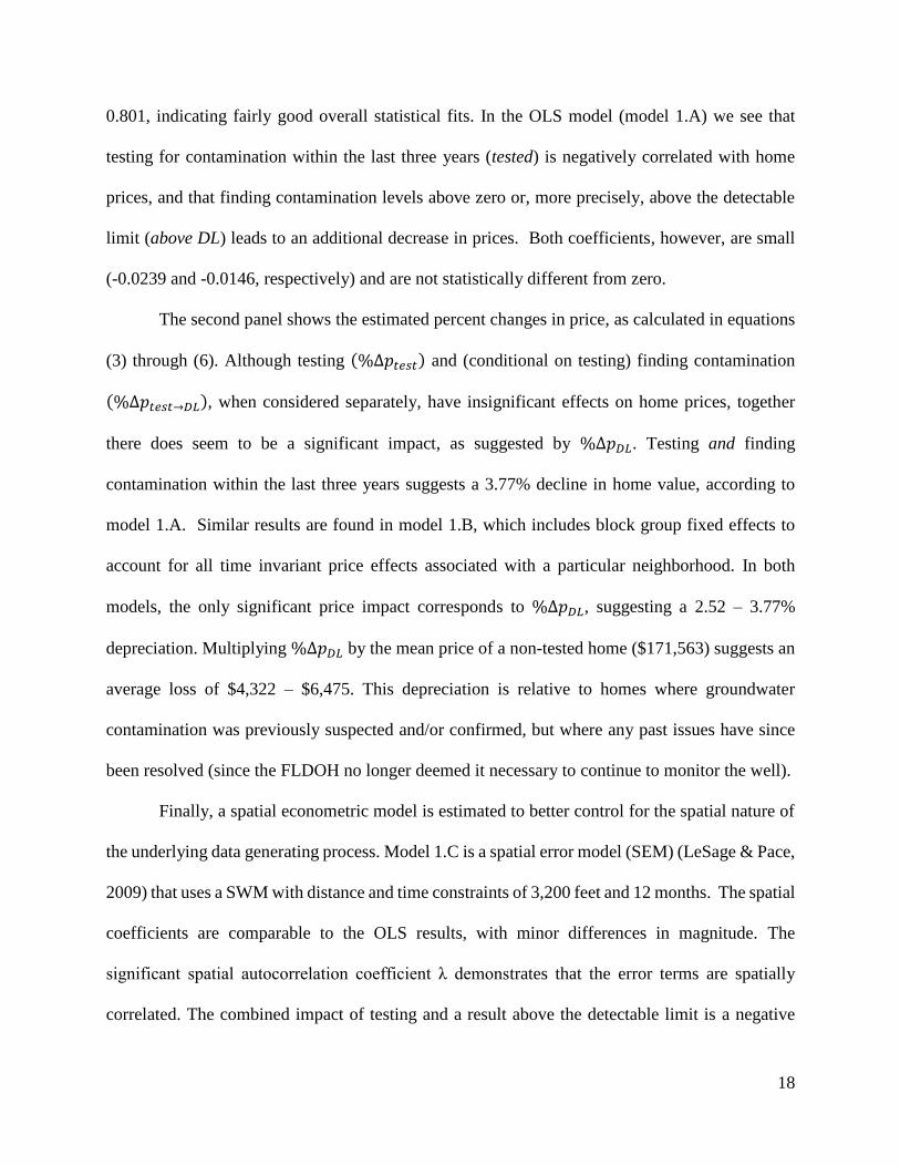
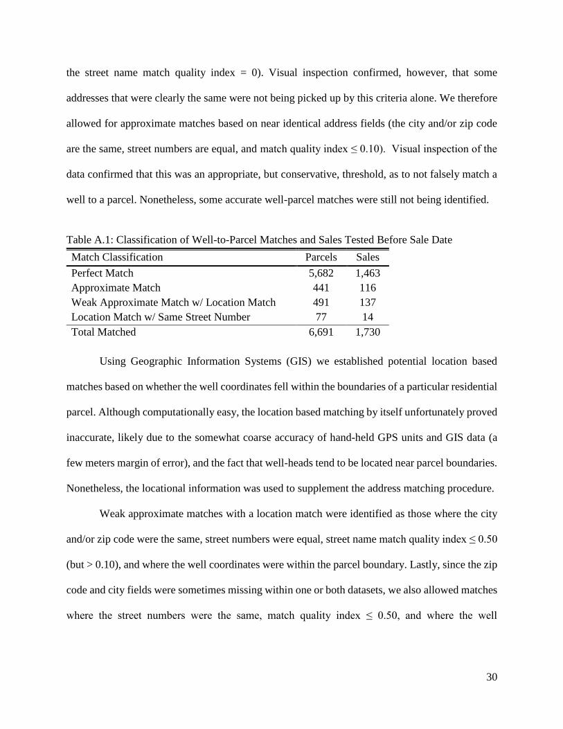NCEE Working Paper Series Working Paper 15-05

November 2015

DISCLAIMER

The views expressed in this paper are those of the author(s) and do not necessarily represent those

of the US Environmental Protection Agency In addition although the research described in this

paper may have been funded entirely or in part by the US Environmental Protection Agency it

has not been subjected to the Agencys required peer and policy review No official Agency

endorsement should be inferred





Abstract








twice the standard




Mail Code 1809 T



Ph 01-202-566-1573

guignetdennisepagov


water quality







INTRODUCTION


















on home prices





1


















concentrations






2

LITERATURE REVIEW






















3
























4























5
























6



EMPIRICAL MODEL



















7

















variables





8























9






provided)


















10
























11




6 process

DATA

















12























was tested


13




















14























15
























16



RESULTS














on March 26 2015)





home

17
























18


level




















19









3 years earlier














20


















estimated as





21






CONCLUSION

















22
























23










24

FIGURES AND TABLES





25









Before Sale Date

Tested 413 615 793 1730




Prior to Sale


ppb ppb ppb ppb


(N+N) 477 3746187 15 22000 10000


Arsenic 22 40706 01160 236 10

26



Price of home (2013$ USD) 1730 2159772 1076671 20000 525000

Age of home (years) 1701 125332 153015 0 123



Lot size (acres) 956 21009 24005 01251 1516



Pool 1730 03260 04689 0 1




Waterfront home 1730 01156 03198 0 1









otherwise noted


27




Tested

times Above DL

times Above MCL

lambda (λ)

-00239

(0019)

-00146

(0018)

00021

(0019)

-00276

(0017)

-00220

(00172)

-00150

(00182)

01040

(00145)

-00239

(0019)

-00145

(0018)

-00007

(0040)

00020

(0019)

-00288

(0018)

00153

(0038)

-00220

(00172)

-00150

(00185)

-00004

(00367)

01040

(00145)

ቲሖኢኰ

ቲሖኢኰሦኇ

ቲሖኇ

ቲሖነኆ

-236

(184)

-145

(179)

-377

(132)

021

(189)

-273

(168)

-252

(123)

-217

(168)

-149

(179)

-363

131

-236

(184)

-144

(178)

-377

(135)

-007

(400)

020

(189)

-284

(172)

-265

(133)

155

(385)

-217

168

-149

(182)

-363

135

-366

347

Observations

Block Group FE

of FEs

1730

No

-

1730

Yes

65

1730

No

-

1730

No

-

1730

Yes

65

1730

No

-






plt001 plt005 plt01

28
























29

























30


equivalent







31

References



101080096405682013772504



Economics 28(1) 43-63 doi 1059500738-1360-28143




1010292009wr008074











32







Journal 65(3) 279-285















df

33





















348

34



283-298










482-493










59

35



















doi 101007s10640-015-9892-2



36





Abstract








twice the standard




Mail Code 1809 T



Ph 01-202-566-1573

guignetdennisepagov


water quality







INTRODUCTION


















on home prices





1


















concentrations






2

LITERATURE REVIEW






















3
























4























5
























6



EMPIRICAL MODEL



















7

















variables





8























9






provided)


















10
























11




6 process

DATA

















12























was tested


13




















14























15
























16



RESULTS














on March 26 2015)





home

17
























18


level




















19









3 years earlier














20


















estimated as





21






CONCLUSION

















22
























23










24

FIGURES AND TABLES





25









Before Sale Date

Tested 413 615 793 1730




Prior to Sale


ppb ppb ppb ppb


(N+N) 477 3746187 15 22000 10000


Arsenic 22 40706 01160 236 10

26



Price of home (2013$ USD) 1730 2159772 1076671 20000 525000

Age of home (years) 1701 125332 153015 0 123



Lot size (acres) 956 21009 24005 01251 1516



Pool 1730 03260 04689 0 1




Waterfront home 1730 01156 03198 0 1









otherwise noted


27




Tested

times Above DL

times Above MCL

lambda (λ)

-00239

(0019)

-00146

(0018)

00021

(0019)

-00276

(0017)

-00220

(00172)

-00150

(00182)

01040

(00145)

-00239

(0019)

-00145

(0018)

-00007

(0040)

00020

(0019)

-00288

(0018)

00153

(0038)

-00220

(00172)

-00150

(00185)

-00004

(00367)

01040

(00145)

ቲሖኢኰ

ቲሖኢኰሦኇ

ቲሖኇ

ቲሖነኆ

-236

(184)

-145

(179)

-377

(132)

021

(189)

-273

(168)

-252

(123)

-217

(168)

-149

(179)

-363

131

-236

(184)

-144

(178)

-377

(135)

-007

(400)

020

(189)

-284

(172)

-265

(133)

155

(385)

-217

168

-149

(182)

-363

135

-366

347

Observations

Block Group FE

of FEs

1730

No

-

1730

Yes

65

1730

No

-

1730

No

-

1730

Yes

65

1730

No

-






plt001 plt005 plt01

28
























29

























30


equivalent







31

References



101080096405682013772504



Economics 28(1) 43-63 doi 1059500738-1360-28143




1010292009wr008074











32







Journal 65(3) 279-285















df

33





















348

34



283-298










482-493










59

35



















doi 101007s10640-015-9892-2



36

INTRODUCTION


















on home prices





1


















concentrations






2

LITERATURE REVIEW






















3
























4























5
























6



EMPIRICAL MODEL



















7

















variables





8























9






provided)


















10
























11




6 process

DATA

















12























was tested


13




















14























15
























16



RESULTS














on March 26 2015)





home

17
























18


level




















19









3 years earlier














20


















estimated as





21






CONCLUSION

















22
























23










24

FIGURES AND TABLES





25









Before Sale Date

Tested 413 615 793 1730




Prior to Sale


ppb ppb ppb ppb


(N+N) 477 3746187 15 22000 10000


Arsenic 22 40706 01160 236 10

26



Price of home (2013$ USD) 1730 2159772 1076671 20000 525000

Age of home (years) 1701 125332 153015 0 123



Lot size (acres) 956 21009 24005 01251 1516



Pool 1730 03260 04689 0 1




Waterfront home 1730 01156 03198 0 1









otherwise noted


27




Tested

times Above DL

times Above MCL

lambda (λ)

-00239

(0019)

-00146

(0018)

00021

(0019)

-00276

(0017)

-00220

(00172)

-00150

(00182)

01040

(00145)

-00239

(0019)

-00145

(0018)

-00007

(0040)

00020

(0019)

-00288

(0018)

00153

(0038)

-00220

(00172)

-00150

(00185)

-00004

(00367)

01040

(00145)

ቲሖኢኰ

ቲሖኢኰሦኇ

ቲሖኇ

ቲሖነኆ

-236

(184)

-145

(179)

-377

(132)

021

(189)

-273

(168)

-252

(123)

-217

(168)

-149

(179)

-363

131

-236

(184)

-144

(178)

-377

(135)

-007

(400)

020

(189)

-284

(172)

-265

(133)

155

(385)

-217

168

-149

(182)

-363

135

-366

347

Observations

Block Group FE

of FEs

1730

No

-

1730

Yes

65

1730

No

-

1730

No

-

1730

Yes

65

1730

No

-






plt001 plt005 plt01

28
























29

























30


equivalent







31

References



101080096405682013772504



Economics 28(1) 43-63 doi 1059500738-1360-28143




1010292009wr008074











32







Journal 65(3) 279-285















df

33





















348

34



283-298










482-493










59

35



















doi 101007s10640-015-9892-2



36


















concentrations






2

LITERATURE REVIEW






















3
























4























5
























6



EMPIRICAL MODEL



















7

















variables





8























9






provided)


















10
























11




6 process

DATA

















12























was tested


13




















14























15
























16



RESULTS














on March 26 2015)





home

17
























18


level




















19









3 years earlier














20


















estimated as





21






CONCLUSION

















22
























23










24

FIGURES AND TABLES





25









Before Sale Date

Tested 413 615 793 1730




Prior to Sale


ppb ppb ppb ppb


(N+N) 477 3746187 15 22000 10000


Arsenic 22 40706 01160 236 10

26



Price of home (2013$ USD) 1730 2159772 1076671 20000 525000

Age of home (years) 1701 125332 153015 0 123



Lot size (acres) 956 21009 24005 01251 1516



Pool 1730 03260 04689 0 1




Waterfront home 1730 01156 03198 0 1









otherwise noted


27




Tested

times Above DL

times Above MCL

lambda (λ)

-00239

(0019)

-00146

(0018)

00021

(0019)

-00276

(0017)

-00220

(00172)

-00150

(00182)

01040

(00145)

-00239

(0019)

-00145

(0018)

-00007

(0040)

00020

(0019)

-00288

(0018)

00153

(0038)

-00220

(00172)

-00150

(00185)

-00004

(00367)

01040

(00145)

ቲሖኢኰ

ቲሖኢኰሦኇ

ቲሖኇ

ቲሖነኆ

-236

(184)

-145

(179)

-377

(132)

021

(189)

-273

(168)

-252

(123)

-217

(168)

-149

(179)

-363

131

-236

(184)

-144

(178)

-377

(135)

-007

(400)

020

(189)

-284

(172)

-265

(133)

155

(385)

-217

168

-149

(182)

-363

135

-366

347

Observations

Block Group FE

of FEs

1730

No

-

1730

Yes

65

1730

No

-

1730

No

-

1730

Yes

65

1730

No

-






plt001 plt005 plt01

28
























29

























30


equivalent







31

References



101080096405682013772504



Economics 28(1) 43-63 doi 1059500738-1360-28143




1010292009wr008074











32







Journal 65(3) 279-285















df

33





















348

34



283-298










482-493










59

35



















doi 101007s10640-015-9892-2



36

LITERATURE REVIEW






















3
























4























5
























6



EMPIRICAL MODEL



















7

















variables





8























9






provided)


















10
























11




6 process

DATA

















12























was tested


13




















14























15
























16



RESULTS














on March 26 2015)





home

17
























18


level




















19









3 years earlier














20


















estimated as





21






CONCLUSION

















22
























23










24

FIGURES AND TABLES





25









Before Sale Date

Tested 413 615 793 1730




Prior to Sale


ppb ppb ppb ppb


(N+N) 477 3746187 15 22000 10000


Arsenic 22 40706 01160 236 10

26



Price of home (2013$ USD) 1730 2159772 1076671 20000 525000

Age of home (years) 1701 125332 153015 0 123



Lot size (acres) 956 21009 24005 01251 1516



Pool 1730 03260 04689 0 1




Waterfront home 1730 01156 03198 0 1









otherwise noted


27




Tested

times Above DL

times Above MCL

lambda (λ)

-00239

(0019)

-00146

(0018)

00021

(0019)

-00276

(0017)

-00220

(00172)

-00150

(00182)

01040

(00145)

-00239

(0019)

-00145

(0018)

-00007

(0040)

00020

(0019)

-00288

(0018)

00153

(0038)

-00220

(00172)

-00150

(00185)

-00004

(00367)

01040

(00145)

ቲሖኢኰ

ቲሖኢኰሦኇ

ቲሖኇ

ቲሖነኆ

-236

(184)

-145

(179)

-377

(132)

021

(189)

-273

(168)

-252

(123)

-217

(168)

-149

(179)

-363

131

-236

(184)

-144

(178)

-377

(135)

-007

(400)

020

(189)

-284

(172)

-265

(133)

155

(385)

-217

168

-149

(182)

-363

135

-366

347

Observations

Block Group FE

of FEs

1730

No

-

1730

Yes

65

1730

No

-

1730

No

-

1730

Yes

65

1730

No

-






plt001 plt005 plt01

28
























29

























30


equivalent







31

References



101080096405682013772504



Economics 28(1) 43-63 doi 1059500738-1360-28143




1010292009wr008074











32







Journal 65(3) 279-285















df

33





















348

34



283-298










482-493










59

35



















doi 101007s10640-015-9892-2



36
























4























5
























6



EMPIRICAL MODEL



















7

















variables





8























9






provided)


















10
























11




6 process

DATA

















12























was tested


13




















14























15
























16



RESULTS














on March 26 2015)





home

17
























18


level




















19









3 years earlier














20


















estimated as





21






CONCLUSION

















22
























23










24

FIGURES AND TABLES





25









Before Sale Date

Tested 413 615 793 1730




Prior to Sale


ppb ppb ppb ppb


(N+N) 477 3746187 15 22000 10000


Arsenic 22 40706 01160 236 10

26



Price of home (2013$ USD) 1730 2159772 1076671 20000 525000

Age of home (years) 1701 125332 153015 0 123



Lot size (acres) 956 21009 24005 01251 1516



Pool 1730 03260 04689 0 1




Waterfront home 1730 01156 03198 0 1









otherwise noted


27




Tested

times Above DL

times Above MCL

lambda (λ)

-00239

(0019)

-00146

(0018)

00021

(0019)

-00276

(0017)

-00220

(00172)

-00150

(00182)

01040

(00145)

-00239

(0019)

-00145

(0018)

-00007

(0040)

00020

(0019)

-00288

(0018)

00153

(0038)

-00220

(00172)

-00150

(00185)

-00004

(00367)

01040

(00145)

ቲሖኢኰ

ቲሖኢኰሦኇ

ቲሖኇ

ቲሖነኆ

-236

(184)

-145

(179)

-377

(132)

021

(189)

-273

(168)

-252

(123)

-217

(168)

-149

(179)

-363

131

-236

(184)

-144

(178)

-377

(135)

-007

(400)

020

(189)

-284

(172)

-265

(133)

155

(385)

-217

168

-149

(182)

-363

135

-366

347

Observations

Block Group FE

of FEs

1730

No

-

1730

Yes

65

1730

No

-

1730

No

-

1730

Yes

65

1730

No

-






plt001 plt005 plt01

28
























29

























30


equivalent







31

References



101080096405682013772504



Economics 28(1) 43-63 doi 1059500738-1360-28143




1010292009wr008074











32







Journal 65(3) 279-285















df

33





















348

34



283-298










482-493










59

35



















doi 101007s10640-015-9892-2



36























5
























6



EMPIRICAL MODEL



















7

















variables





8























9






provided)


















10
























11




6 process

DATA

















12























was tested


13




















14























15
























16



RESULTS














on March 26 2015)





home

17
























18


level




















19









3 years earlier














20


















estimated as





21






CONCLUSION

















22
























23










24

FIGURES AND TABLES





25









Before Sale Date

Tested 413 615 793 1730




Prior to Sale


ppb ppb ppb ppb


(N+N) 477 3746187 15 22000 10000


Arsenic 22 40706 01160 236 10

26



Price of home (2013$ USD) 1730 2159772 1076671 20000 525000

Age of home (years) 1701 125332 153015 0 123



Lot size (acres) 956 21009 24005 01251 1516



Pool 1730 03260 04689 0 1




Waterfront home 1730 01156 03198 0 1









otherwise noted


27




Tested

times Above DL

times Above MCL

lambda (λ)

-00239

(0019)

-00146

(0018)

00021

(0019)

-00276

(0017)

-00220

(00172)

-00150

(00182)

01040

(00145)

-00239

(0019)

-00145

(0018)

-00007

(0040)

00020

(0019)

-00288

(0018)

00153

(0038)

-00220

(00172)

-00150

(00185)

-00004

(00367)

01040

(00145)

ቲሖኢኰ

ቲሖኢኰሦኇ

ቲሖኇ

ቲሖነኆ

-236

(184)

-145

(179)

-377

(132)

021

(189)

-273

(168)

-252

(123)

-217

(168)

-149

(179)

-363

131

-236

(184)

-144

(178)

-377

(135)

-007

(400)

020

(189)

-284

(172)

-265

(133)

155

(385)

-217

168

-149

(182)

-363

135

-366

347

Observations

Block Group FE

of FEs

1730

No

-

1730

Yes

65

1730

No

-

1730

No

-

1730

Yes

65

1730

No

-






plt001 plt005 plt01

28
























29

























30


equivalent







31

References



101080096405682013772504



Economics 28(1) 43-63 doi 1059500738-1360-28143




1010292009wr008074











32







Journal 65(3) 279-285















df

33





















348

34



283-298










482-493










59

35



















doi 101007s10640-015-9892-2



36
























6



EMPIRICAL MODEL



















7

















variables





8























9






provided)


















10
























11




6 process

DATA

















12























was tested


13




















14























15
























16



RESULTS














on March 26 2015)





home

17
























18


level




















19









3 years earlier














20


















estimated as





21






CONCLUSION

















22
























23










24

FIGURES AND TABLES





25









Before Sale Date

Tested 413 615 793 1730




Prior to Sale


ppb ppb ppb ppb


(N+N) 477 3746187 15 22000 10000


Arsenic 22 40706 01160 236 10

26



Price of home (2013$ USD) 1730 2159772 1076671 20000 525000

Age of home (years) 1701 125332 153015 0 123



Lot size (acres) 956 21009 24005 01251 1516



Pool 1730 03260 04689 0 1




Waterfront home 1730 01156 03198 0 1









otherwise noted


27




Tested

times Above DL

times Above MCL

lambda (λ)

-00239

(0019)

-00146

(0018)

00021

(0019)

-00276

(0017)

-00220

(00172)

-00150

(00182)

01040

(00145)

-00239

(0019)

-00145

(0018)

-00007

(0040)

00020

(0019)

-00288

(0018)

00153

(0038)

-00220

(00172)

-00150

(00185)

-00004

(00367)

01040

(00145)

ቲሖኢኰ

ቲሖኢኰሦኇ

ቲሖኇ

ቲሖነኆ

-236

(184)

-145

(179)

-377

(132)

021

(189)

-273

(168)

-252

(123)

-217

(168)

-149

(179)

-363

131

-236

(184)

-144

(178)

-377

(135)

-007

(400)

020

(189)

-284

(172)

-265

(133)

155

(385)

-217

168

-149

(182)

-363

135

-366

347

Observations

Block Group FE

of FEs

1730

No

-

1730

Yes

65

1730

No

-

1730

No

-

1730

Yes

65

1730

No

-






plt001 plt005 plt01

28
























29

























30


equivalent







31

References



101080096405682013772504



Economics 28(1) 43-63 doi 1059500738-1360-28143




1010292009wr008074











32







Journal 65(3) 279-285















df

33





















348

34



283-298










482-493










59

35



















doi 101007s10640-015-9892-2



36



EMPIRICAL MODEL



















7

















variables





8























9






provided)


















10
























11




6 process

DATA

















12























was tested


13




















14























15
























16



RESULTS














on March 26 2015)





home

17
























18


level




















19









3 years earlier














20


















estimated as





21






CONCLUSION

















22
























23










24

FIGURES AND TABLES





25









Before Sale Date

Tested 413 615 793 1730




Prior to Sale


ppb ppb ppb ppb


(N+N) 477 3746187 15 22000 10000


Arsenic 22 40706 01160 236 10

26



Price of home (2013$ USD) 1730 2159772 1076671 20000 525000

Age of home (years) 1701 125332 153015 0 123



Lot size (acres) 956 21009 24005 01251 1516



Pool 1730 03260 04689 0 1




Waterfront home 1730 01156 03198 0 1









otherwise noted


27




Tested

times Above DL

times Above MCL

lambda (λ)

-00239

(0019)

-00146

(0018)

00021

(0019)

-00276

(0017)

-00220

(00172)

-00150

(00182)

01040

(00145)

-00239

(0019)

-00145

(0018)

-00007

(0040)

00020

(0019)

-00288

(0018)

00153

(0038)

-00220

(00172)

-00150

(00185)

-00004

(00367)

01040

(00145)

ቲሖኢኰ

ቲሖኢኰሦኇ

ቲሖኇ

ቲሖነኆ

-236

(184)

-145

(179)

-377

(132)

021

(189)

-273

(168)

-252

(123)

-217

(168)

-149

(179)

-363

131

-236

(184)

-144

(178)

-377

(135)

-007

(400)

020

(189)

-284

(172)

-265

(133)

155

(385)

-217

168

-149

(182)

-363

135

-366

347

Observations

Block Group FE

of FEs

1730

No

-

1730

Yes

65

1730

No

-

1730

No

-

1730

Yes

65

1730

No

-






plt001 plt005 plt01

28
























29

























30


equivalent







31

References



101080096405682013772504



Economics 28(1) 43-63 doi 1059500738-1360-28143




1010292009wr008074











32







Journal 65(3) 279-285















df

33





















348

34



283-298










482-493










59

35



















doi 101007s10640-015-9892-2



36

















variables





8























9






provided)


















10
























11




6 process

DATA

















12























was tested


13




















14























15
























16



RESULTS














on March 26 2015)





home

17
























18


level




















19









3 years earlier














20


















estimated as





21






CONCLUSION

















22
























23










24

FIGURES AND TABLES





25









Before Sale Date

Tested 413 615 793 1730




Prior to Sale


ppb ppb ppb ppb


(N+N) 477 3746187 15 22000 10000


Arsenic 22 40706 01160 236 10

26



Price of home (2013$ USD) 1730 2159772 1076671 20000 525000

Age of home (years) 1701 125332 153015 0 123



Lot size (acres) 956 21009 24005 01251 1516



Pool 1730 03260 04689 0 1




Waterfront home 1730 01156 03198 0 1









otherwise noted


27




Tested

times Above DL

times Above MCL

lambda (λ)

-00239

(0019)

-00146

(0018)

00021

(0019)

-00276

(0017)

-00220

(00172)

-00150

(00182)

01040

(00145)

-00239

(0019)

-00145

(0018)

-00007

(0040)

00020

(0019)

-00288

(0018)

00153

(0038)

-00220

(00172)

-00150

(00185)

-00004

(00367)

01040

(00145)

ቲሖኢኰ

ቲሖኢኰሦኇ

ቲሖኇ

ቲሖነኆ

-236

(184)

-145

(179)

-377

(132)

021

(189)

-273

(168)

-252

(123)

-217

(168)

-149

(179)

-363

131

-236

(184)

-144

(178)

-377

(135)

-007

(400)

020

(189)

-284

(172)

-265

(133)

155

(385)

-217

168

-149

(182)

-363

135

-366

347

Observations

Block Group FE

of FEs

1730

No

-

1730

Yes

65

1730

No

-

1730

No

-

1730

Yes

65

1730

No

-






plt001 plt005 plt01

28
























29

























30


equivalent







31

References



101080096405682013772504



Economics 28(1) 43-63 doi 1059500738-1360-28143




1010292009wr008074











32







Journal 65(3) 279-285















df

33





















348

34



283-298










482-493










59

35



















doi 101007s10640-015-9892-2



36























9






provided)


















10
























11




6 process

DATA

















12























was tested


13




















14























15
























16



RESULTS














on March 26 2015)





home

17
























18


level




















19









3 years earlier














20


















estimated as





21






CONCLUSION

















22
























23










24

FIGURES AND TABLES





25









Before Sale Date

Tested 413 615 793 1730




Prior to Sale


ppb ppb ppb ppb


(N+N) 477 3746187 15 22000 10000


Arsenic 22 40706 01160 236 10

26



Price of home (2013$ USD) 1730 2159772 1076671 20000 525000

Age of home (years) 1701 125332 153015 0 123



Lot size (acres) 956 21009 24005 01251 1516



Pool 1730 03260 04689 0 1




Waterfront home 1730 01156 03198 0 1









otherwise noted


27




Tested

times Above DL

times Above MCL

lambda (λ)

-00239

(0019)

-00146

(0018)

00021

(0019)

-00276

(0017)

-00220

(00172)

-00150

(00182)

01040

(00145)

-00239

(0019)

-00145

(0018)

-00007

(0040)

00020

(0019)

-00288

(0018)

00153

(0038)

-00220

(00172)

-00150

(00185)

-00004

(00367)

01040

(00145)

ቲሖኢኰ

ቲሖኢኰሦኇ

ቲሖኇ

ቲሖነኆ

-236

(184)

-145

(179)

-377

(132)

021

(189)

-273

(168)

-252

(123)

-217

(168)

-149

(179)

-363

131

-236

(184)

-144

(178)

-377

(135)

-007

(400)

020

(189)

-284

(172)

-265

(133)

155

(385)

-217

168

-149

(182)

-363

135

-366

347

Observations

Block Group FE

of FEs

1730

No

-

1730

Yes

65

1730

No

-

1730

No

-

1730

Yes

65

1730

No

-






plt001 plt005 plt01

28
























29

























30


equivalent







31

References



101080096405682013772504



Economics 28(1) 43-63 doi 1059500738-1360-28143




1010292009wr008074











32







Journal 65(3) 279-285















df

33





















348

34



283-298










482-493










59

35



















doi 101007s10640-015-9892-2



36






provided)


















10
























11




6 process

DATA

















12























was tested


13




















14























15
























16



RESULTS














on March 26 2015)





home

17
























18


level




















19









3 years earlier














20


















estimated as





21






CONCLUSION

















22
























23










24

FIGURES AND TABLES





25









Before Sale Date

Tested 413 615 793 1730




Prior to Sale


ppb ppb ppb ppb


(N+N) 477 3746187 15 22000 10000


Arsenic 22 40706 01160 236 10

26



Price of home (2013$ USD) 1730 2159772 1076671 20000 525000

Age of home (years) 1701 125332 153015 0 123



Lot size (acres) 956 21009 24005 01251 1516



Pool 1730 03260 04689 0 1




Waterfront home 1730 01156 03198 0 1









otherwise noted


27




Tested

times Above DL

times Above MCL

lambda (λ)

-00239

(0019)

-00146

(0018)

00021

(0019)

-00276

(0017)

-00220

(00172)

-00150

(00182)

01040

(00145)

-00239

(0019)

-00145

(0018)

-00007

(0040)

00020

(0019)

-00288

(0018)

00153

(0038)

-00220

(00172)

-00150

(00185)

-00004

(00367)

01040

(00145)

ቲሖኢኰ

ቲሖኢኰሦኇ

ቲሖኇ

ቲሖነኆ

-236

(184)

-145

(179)

-377

(132)

021

(189)

-273

(168)

-252

(123)

-217

(168)

-149

(179)

-363

131

-236

(184)

-144

(178)

-377

(135)

-007

(400)

020

(189)

-284

(172)

-265

(133)

155

(385)

-217

168

-149

(182)

-363

135

-366

347

Observations

Block Group FE

of FEs

1730

No

-

1730

Yes

65

1730

No

-

1730

No

-

1730

Yes

65

1730

No

-






plt001 plt005 plt01

28
























29

























30


equivalent







31

References



101080096405682013772504



Economics 28(1) 43-63 doi 1059500738-1360-28143




1010292009wr008074











32







Journal 65(3) 279-285















df

33





















348

34



283-298










482-493










59

35



















doi 101007s10640-015-9892-2



36
























11




6 process

DATA

















12























was tested


13




















14























15
























16



RESULTS














on March 26 2015)





home

17
























18


level




















19









3 years earlier














20


















estimated as





21






CONCLUSION

















22
























23










24

FIGURES AND TABLES





25









Before Sale Date

Tested 413 615 793 1730




Prior to Sale


ppb ppb ppb ppb


(N+N) 477 3746187 15 22000 10000


Arsenic 22 40706 01160 236 10

26



Price of home (2013$ USD) 1730 2159772 1076671 20000 525000

Age of home (years) 1701 125332 153015 0 123



Lot size (acres) 956 21009 24005 01251 1516



Pool 1730 03260 04689 0 1




Waterfront home 1730 01156 03198 0 1









otherwise noted


27




Tested

times Above DL

times Above MCL

lambda (λ)

-00239

(0019)

-00146

(0018)

00021

(0019)

-00276

(0017)

-00220

(00172)

-00150

(00182)

01040

(00145)

-00239

(0019)

-00145

(0018)

-00007

(0040)

00020

(0019)

-00288

(0018)

00153

(0038)

-00220

(00172)

-00150

(00185)

-00004

(00367)

01040

(00145)

ቲሖኢኰ

ቲሖኢኰሦኇ

ቲሖኇ

ቲሖነኆ

-236

(184)

-145

(179)

-377

(132)

021

(189)

-273

(168)

-252

(123)

-217

(168)

-149

(179)

-363

131

-236

(184)

-144

(178)

-377

(135)

-007

(400)

020

(189)

-284

(172)

-265

(133)

155

(385)

-217

168

-149

(182)

-363

135

-366

347

Observations

Block Group FE

of FEs

1730

No

-

1730

Yes

65

1730

No

-

1730

No

-

1730

Yes

65

1730

No

-






plt001 plt005 plt01

28
























29

























30


equivalent







31

References



101080096405682013772504



Economics 28(1) 43-63 doi 1059500738-1360-28143




1010292009wr008074











32







Journal 65(3) 279-285















df

33





















348

34



283-298










482-493










59

35



















doi 101007s10640-015-9892-2



36




6 process

DATA

















12























was tested


13




















14























15
























16



RESULTS














on March 26 2015)





home

17
























18


level




















19









3 years earlier














20


















estimated as





21






CONCLUSION

















22
























23










24

FIGURES AND TABLES





25









Before Sale Date

Tested 413 615 793 1730




Prior to Sale


ppb ppb ppb ppb


(N+N) 477 3746187 15 22000 10000


Arsenic 22 40706 01160 236 10

26



Price of home (2013$ USD) 1730 2159772 1076671 20000 525000

Age of home (years) 1701 125332 153015 0 123



Lot size (acres) 956 21009 24005 01251 1516



Pool 1730 03260 04689 0 1




Waterfront home 1730 01156 03198 0 1









otherwise noted


27




Tested

times Above DL

times Above MCL

lambda (λ)

-00239

(0019)

-00146

(0018)

00021

(0019)

-00276

(0017)

-00220

(00172)

-00150

(00182)

01040

(00145)

-00239

(0019)

-00145

(0018)

-00007

(0040)

00020

(0019)

-00288

(0018)

00153

(0038)

-00220

(00172)

-00150

(00185)

-00004

(00367)

01040

(00145)

ቲሖኢኰ

ቲሖኢኰሦኇ

ቲሖኇ

ቲሖነኆ

-236

(184)

-145

(179)

-377

(132)

021

(189)

-273

(168)

-252

(123)

-217

(168)

-149

(179)

-363

131

-236

(184)

-144

(178)

-377

(135)

-007

(400)

020

(189)

-284

(172)

-265

(133)

155

(385)

-217

168

-149

(182)

-363

135

-366

347

Observations

Block Group FE

of FEs

1730

No

-

1730

Yes

65

1730

No

-

1730

No

-

1730

Yes

65

1730

No

-






plt001 plt005 plt01

28
























29

























30


equivalent







31

References



101080096405682013772504



Economics 28(1) 43-63 doi 1059500738-1360-28143




1010292009wr008074











32







Journal 65(3) 279-285















df

33





















348

34



283-298










482-493










59

35



















doi 101007s10640-015-9892-2



36























was tested


13




















14























15
























16



RESULTS














on March 26 2015)





home

17
























18


level




















19









3 years earlier














20


















estimated as





21






CONCLUSION

















22
























23










24

FIGURES AND TABLES





25









Before Sale Date

Tested 413 615 793 1730




Prior to Sale


ppb ppb ppb ppb


(N+N) 477 3746187 15 22000 10000


Arsenic 22 40706 01160 236 10

26



Price of home (2013$ USD) 1730 2159772 1076671 20000 525000

Age of home (years) 1701 125332 153015 0 123



Lot size (acres) 956 21009 24005 01251 1516



Pool 1730 03260 04689 0 1




Waterfront home 1730 01156 03198 0 1









otherwise noted


27




Tested

times Above DL

times Above MCL

lambda (λ)

-00239

(0019)

-00146

(0018)

00021

(0019)

-00276

(0017)

-00220

(00172)

-00150

(00182)

01040

(00145)

-00239

(0019)

-00145

(0018)

-00007

(0040)

00020

(0019)

-00288

(0018)

00153

(0038)

-00220

(00172)

-00150

(00185)

-00004

(00367)

01040

(00145)

ቲሖኢኰ

ቲሖኢኰሦኇ

ቲሖኇ

ቲሖነኆ

-236

(184)

-145

(179)

-377

(132)

021

(189)

-273

(168)

-252

(123)

-217

(168)

-149

(179)

-363

131

-236

(184)

-144

(178)

-377

(135)

-007

(400)

020

(189)

-284

(172)

-265

(133)

155

(385)

-217

168

-149

(182)

-363

135

-366

347

Observations

Block Group FE

of FEs

1730

No

-

1730

Yes

65

1730

No

-

1730

No

-

1730

Yes

65

1730

No

-






plt001 plt005 plt01

28
























29

























30


equivalent







31

References



101080096405682013772504



Economics 28(1) 43-63 doi 1059500738-1360-28143




1010292009wr008074











32







Journal 65(3) 279-285















df

33





















348

34



283-298










482-493










59

35



















doi 101007s10640-015-9892-2



36




















14























15
























16



RESULTS














on March 26 2015)





home

17
























18


level




















19









3 years earlier














20


















estimated as





21






CONCLUSION

















22
























23










24

FIGURES AND TABLES





25









Before Sale Date

Tested 413 615 793 1730




Prior to Sale


ppb ppb ppb ppb


(N+N) 477 3746187 15 22000 10000


Arsenic 22 40706 01160 236 10

26



Price of home (2013$ USD) 1730 2159772 1076671 20000 525000

Age of home (years) 1701 125332 153015 0 123



Lot size (acres) 956 21009 24005 01251 1516



Pool 1730 03260 04689 0 1




Waterfront home 1730 01156 03198 0 1









otherwise noted


27




Tested

times Above DL

times Above MCL

lambda (λ)

-00239

(0019)

-00146

(0018)

00021

(0019)

-00276

(0017)

-00220

(00172)

-00150

(00182)

01040

(00145)

-00239

(0019)

-00145

(0018)

-00007

(0040)

00020

(0019)

-00288

(0018)

00153

(0038)

-00220

(00172)

-00150

(00185)

-00004

(00367)

01040

(00145)

ቲሖኢኰ

ቲሖኢኰሦኇ

ቲሖኇ

ቲሖነኆ

-236

(184)

-145

(179)

-377

(132)

021

(189)

-273

(168)

-252

(123)

-217

(168)

-149

(179)

-363

131

-236

(184)

-144

(178)

-377

(135)

-007

(400)

020

(189)

-284

(172)

-265

(133)

155

(385)

-217

168

-149

(182)

-363

135

-366

347

Observations

Block Group FE

of FEs

1730

No

-

1730

Yes

65

1730

No

-

1730

No

-

1730

Yes

65

1730

No

-






plt001 plt005 plt01

28
























29

























30


equivalent







31

References



101080096405682013772504



Economics 28(1) 43-63 doi 1059500738-1360-28143




1010292009wr008074











32







Journal 65(3) 279-285















df

33





















348

34



283-298










482-493










59

35



















doi 101007s10640-015-9892-2



36























15
























16



RESULTS














on March 26 2015)





home

17
























18


level




















19









3 years earlier














20


















estimated as





21






CONCLUSION

















22
























23










24

FIGURES AND TABLES





25









Before Sale Date

Tested 413 615 793 1730




Prior to Sale


ppb ppb ppb ppb


(N+N) 477 3746187 15 22000 10000


Arsenic 22 40706 01160 236 10

26



Price of home (2013$ USD) 1730 2159772 1076671 20000 525000

Age of home (years) 1701 125332 153015 0 123



Lot size (acres) 956 21009 24005 01251 1516



Pool 1730 03260 04689 0 1




Waterfront home 1730 01156 03198 0 1









otherwise noted


27




Tested

times Above DL

times Above MCL

lambda (λ)

-00239

(0019)

-00146

(0018)

00021

(0019)

-00276

(0017)

-00220

(00172)

-00150

(00182)

01040

(00145)

-00239

(0019)

-00145

(0018)

-00007

(0040)

00020

(0019)

-00288

(0018)

00153

(0038)

-00220

(00172)

-00150

(00185)

-00004

(00367)

01040

(00145)

ቲሖኢኰ

ቲሖኢኰሦኇ

ቲሖኇ

ቲሖነኆ

-236

(184)

-145

(179)

-377

(132)

021

(189)

-273

(168)

-252

(123)

-217

(168)

-149

(179)

-363

131

-236

(184)

-144

(178)

-377

(135)

-007

(400)

020

(189)

-284

(172)

-265

(133)

155

(385)

-217

168

-149

(182)

-363

135

-366

347

Observations

Block Group FE

of FEs

1730

No

-

1730

Yes

65

1730

No

-

1730

No

-

1730

Yes

65

1730

No

-






plt001 plt005 plt01

28
























29

























30


equivalent







31

References



101080096405682013772504



Economics 28(1) 43-63 doi 1059500738-1360-28143




1010292009wr008074











32







Journal 65(3) 279-285















df

33





















348

34



283-298










482-493










59

35



















doi 101007s10640-015-9892-2



36
























16



RESULTS














on March 26 2015)





home

17
























18


level




















19









3 years earlier














20


















estimated as





21






CONCLUSION

















22
























23










24

FIGURES AND TABLES





25









Before Sale Date

Tested 413 615 793 1730




Prior to Sale


ppb ppb ppb ppb


(N+N) 477 3746187 15 22000 10000


Arsenic 22 40706 01160 236 10

26



Price of home (2013$ USD) 1730 2159772 1076671 20000 525000

Age of home (years) 1701 125332 153015 0 123



Lot size (acres) 956 21009 24005 01251 1516



Pool 1730 03260 04689 0 1




Waterfront home 1730 01156 03198 0 1









otherwise noted


27




Tested

times Above DL

times Above MCL

lambda (λ)

-00239

(0019)

-00146

(0018)

00021

(0019)

-00276

(0017)

-00220

(00172)

-00150

(00182)

01040

(00145)

-00239

(0019)

-00145

(0018)

-00007

(0040)

00020

(0019)

-00288

(0018)

00153

(0038)

-00220

(00172)

-00150

(00185)

-00004

(00367)

01040

(00145)

ቲሖኢኰ

ቲሖኢኰሦኇ

ቲሖኇ

ቲሖነኆ

-236

(184)

-145

(179)

-377

(132)

021

(189)

-273

(168)

-252

(123)

-217

(168)

-149

(179)

-363

131

-236

(184)

-144

(178)

-377

(135)

-007

(400)

020

(189)

-284

(172)

-265

(133)

155

(385)

-217

168

-149

(182)

-363

135

-366

347

Observations

Block Group FE

of FEs

1730

No

-

1730

Yes

65

1730

No

-

1730

No

-

1730

Yes

65

1730

No

-






plt001 plt005 plt01

28
























29

























30


equivalent







31

References



101080096405682013772504



Economics 28(1) 43-63 doi 1059500738-1360-28143




1010292009wr008074











32







Journal 65(3) 279-285















df

33





















348

34



283-298










482-493










59

35



















doi 101007s10640-015-9892-2



36



RESULTS














on March 26 2015)





home

17
























18


level




















19









3 years earlier














20


















estimated as





21






CONCLUSION

















22
























23










24

FIGURES AND TABLES





25









Before Sale Date

Tested 413 615 793 1730




Prior to Sale


ppb ppb ppb ppb


(N+N) 477 3746187 15 22000 10000


Arsenic 22 40706 01160 236 10

26



Price of home (2013$ USD) 1730 2159772 1076671 20000 525000

Age of home (years) 1701 125332 153015 0 123



Lot size (acres) 956 21009 24005 01251 1516



Pool 1730 03260 04689 0 1




Waterfront home 1730 01156 03198 0 1









otherwise noted


27




Tested

times Above DL

times Above MCL

lambda (λ)

-00239

(0019)

-00146

(0018)

00021

(0019)

-00276

(0017)

-00220

(00172)

-00150

(00182)

01040

(00145)

-00239

(0019)

-00145

(0018)

-00007

(0040)

00020

(0019)

-00288

(0018)

00153

(0038)

-00220

(00172)

-00150

(00185)

-00004

(00367)

01040

(00145)

ቲሖኢኰ

ቲሖኢኰሦኇ

ቲሖኇ

ቲሖነኆ

-236

(184)

-145

(179)

-377

(132)

021

(189)

-273

(168)

-252

(123)

-217

(168)

-149

(179)

-363

131

-236

(184)

-144

(178)

-377

(135)

-007

(400)

020

(189)

-284

(172)

-265

(133)

155

(385)

-217

168

-149

(182)

-363

135

-366

347

Observations

Block Group FE

of FEs

1730

No

-

1730

Yes

65

1730

No

-

1730

No

-

1730

Yes

65

1730

No

-






plt001 plt005 plt01

28
























29

























30


equivalent







31

References



101080096405682013772504



Economics 28(1) 43-63 doi 1059500738-1360-28143




1010292009wr008074











32







Journal 65(3) 279-285















df

33





















348

34



283-298










482-493










59

35



















doi 101007s10640-015-9892-2



36
























18


level




















19









3 years earlier














20


















estimated as





21






CONCLUSION

















22
























23










24

FIGURES AND TABLES





25









Before Sale Date

Tested 413 615 793 1730




Prior to Sale


ppb ppb ppb ppb


(N+N) 477 3746187 15 22000 10000


Arsenic 22 40706 01160 236 10

26



Price of home (2013$ USD) 1730 2159772 1076671 20000 525000

Age of home (years) 1701 125332 153015 0 123



Lot size (acres) 956 21009 24005 01251 1516



Pool 1730 03260 04689 0 1




Waterfront home 1730 01156 03198 0 1









otherwise noted


27




Tested

times Above DL

times Above MCL

lambda (λ)

-00239

(0019)

-00146

(0018)

00021

(0019)

-00276

(0017)

-00220

(00172)

-00150

(00182)

01040

(00145)

-00239

(0019)

-00145

(0018)

-00007

(0040)

00020

(0019)

-00288

(0018)

00153

(0038)

-00220

(00172)

-00150

(00185)

-00004

(00367)

01040

(00145)

ቲሖኢኰ

ቲሖኢኰሦኇ

ቲሖኇ

ቲሖነኆ

-236

(184)

-145

(179)

-377

(132)

021

(189)

-273

(168)

-252

(123)

-217

(168)

-149

(179)

-363

131

-236

(184)

-144

(178)

-377

(135)

-007

(400)

020

(189)

-284

(172)

-265

(133)

155

(385)

-217

168

-149

(182)

-363

135

-366

347

Observations

Block Group FE

of FEs

1730

No

-

1730

Yes

65

1730

No

-

1730

No

-

1730

Yes

65

1730

No

-






plt001 plt005 plt01

28
























29

























30


equivalent







31

References



101080096405682013772504



Economics 28(1) 43-63 doi 1059500738-1360-28143




1010292009wr008074











32







Journal 65(3) 279-285















df

33





















348

34



283-298










482-493










59

35



















doi 101007s10640-015-9892-2



36


level




















19









3 years earlier














20


















estimated as





21






CONCLUSION

















22
























23










24

FIGURES AND TABLES





25









Before Sale Date

Tested 413 615 793 1730




Prior to Sale


ppb ppb ppb ppb


(N+N) 477 3746187 15 22000 10000


Arsenic 22 40706 01160 236 10

26



Price of home (2013$ USD) 1730 2159772 1076671 20000 525000

Age of home (years) 1701 125332 153015 0 123



Lot size (acres) 956 21009 24005 01251 1516



Pool 1730 03260 04689 0 1




Waterfront home 1730 01156 03198 0 1









otherwise noted


27




Tested

times Above DL

times Above MCL

lambda (λ)

-00239

(0019)

-00146

(0018)

00021

(0019)

-00276

(0017)

-00220

(00172)

-00150

(00182)

01040

(00145)

-00239

(0019)

-00145

(0018)

-00007

(0040)

00020

(0019)

-00288

(0018)

00153

(0038)

-00220

(00172)

-00150

(00185)

-00004

(00367)

01040

(00145)

ቲሖኢኰ

ቲሖኢኰሦኇ

ቲሖኇ

ቲሖነኆ

-236

(184)

-145

(179)

-377

(132)

021

(189)

-273

(168)

-252

(123)

-217

(168)

-149

(179)

-363

131

-236

(184)

-144

(178)

-377

(135)

-007

(400)

020

(189)

-284

(172)

-265

(133)

155

(385)

-217

168

-149

(182)

-363

135

-366

347

Observations

Block Group FE

of FEs

1730

No

-

1730

Yes

65

1730

No

-

1730

No

-

1730

Yes

65

1730

No

-






plt001 plt005 plt01

28
























29

























30


equivalent







31

References



101080096405682013772504



Economics 28(1) 43-63 doi 1059500738-1360-28143




1010292009wr008074











32







Journal 65(3) 279-285















df

33





















348

34



283-298










482-493










59

35



















doi 101007s10640-015-9892-2



36









3 years earlier














20


















estimated as





21






CONCLUSION

















22
























23










24

FIGURES AND TABLES





25









Before Sale Date

Tested 413 615 793 1730




Prior to Sale


ppb ppb ppb ppb


(N+N) 477 3746187 15 22000 10000


Arsenic 22 40706 01160 236 10

26



Price of home (2013$ USD) 1730 2159772 1076671 20000 525000

Age of home (years) 1701 125332 153015 0 123



Lot size (acres) 956 21009 24005 01251 1516



Pool 1730 03260 04689 0 1




Waterfront home 1730 01156 03198 0 1









otherwise noted


27




Tested

times Above DL

times Above MCL

lambda (λ)

-00239

(0019)

-00146

(0018)

00021

(0019)

-00276

(0017)

-00220

(00172)

-00150

(00182)

01040

(00145)

-00239

(0019)

-00145

(0018)

-00007

(0040)

00020

(0019)

-00288

(0018)

00153

(0038)

-00220

(00172)

-00150

(00185)

-00004

(00367)

01040

(00145)

ቲሖኢኰ

ቲሖኢኰሦኇ

ቲሖኇ

ቲሖነኆ

-236

(184)

-145

(179)

-377

(132)

021

(189)

-273

(168)

-252

(123)

-217

(168)

-149

(179)

-363

131

-236

(184)

-144

(178)

-377

(135)

-007

(400)

020

(189)

-284

(172)

-265

(133)

155

(385)

-217

168

-149

(182)

-363

135

-366

347

Observations

Block Group FE

of FEs

1730

No

-

1730

Yes

65

1730

No

-

1730

No

-

1730

Yes

65

1730

No

-






plt001 plt005 plt01

28
























29

























30


equivalent







31

References



101080096405682013772504



Economics 28(1) 43-63 doi 1059500738-1360-28143




1010292009wr008074











32







Journal 65(3) 279-285















df

33





















348

34



283-298










482-493










59

35



















doi 101007s10640-015-9892-2



36


















estimated as





21






CONCLUSION

















22
























23










24

FIGURES AND TABLES





25









Before Sale Date

Tested 413 615 793 1730




Prior to Sale


ppb ppb ppb ppb


(N+N) 477 3746187 15 22000 10000


Arsenic 22 40706 01160 236 10

26



Price of home (2013$ USD) 1730 2159772 1076671 20000 525000

Age of home (years) 1701 125332 153015 0 123



Lot size (acres) 956 21009 24005 01251 1516



Pool 1730 03260 04689 0 1




Waterfront home 1730 01156 03198 0 1









otherwise noted


27




Tested

times Above DL

times Above MCL

lambda (λ)

-00239

(0019)

-00146

(0018)

00021

(0019)

-00276

(0017)

-00220

(00172)

-00150

(00182)

01040

(00145)

-00239

(0019)

-00145

(0018)

-00007

(0040)

00020

(0019)

-00288

(0018)

00153

(0038)

-00220

(00172)

-00150

(00185)

-00004

(00367)

01040

(00145)

ቲሖኢኰ

ቲሖኢኰሦኇ

ቲሖኇ

ቲሖነኆ

-236

(184)

-145

(179)

-377

(132)

021

(189)

-273

(168)

-252

(123)

-217

(168)

-149

(179)

-363

131

-236

(184)

-144

(178)

-377

(135)

-007

(400)

020

(189)

-284

(172)

-265

(133)

155

(385)

-217

168

-149

(182)

-363

135

-366

347

Observations

Block Group FE

of FEs

1730

No

-

1730

Yes

65

1730

No

-

1730

No

-

1730

Yes

65

1730

No

-






plt001 plt005 plt01

28
























29

























30


equivalent







31

References



101080096405682013772504



Economics 28(1) 43-63 doi 1059500738-1360-28143




1010292009wr008074











32







Journal 65(3) 279-285















df

33





















348

34



283-298










482-493










59

35



















doi 101007s10640-015-9892-2



36






CONCLUSION

















22
























23










24

FIGURES AND TABLES





25









Before Sale Date

Tested 413 615 793 1730




Prior to Sale


ppb ppb ppb ppb


(N+N) 477 3746187 15 22000 10000


Arsenic 22 40706 01160 236 10

26



Price of home (2013$ USD) 1730 2159772 1076671 20000 525000

Age of home (years) 1701 125332 153015 0 123



Lot size (acres) 956 21009 24005 01251 1516



Pool 1730 03260 04689 0 1




Waterfront home 1730 01156 03198 0 1









otherwise noted


27




Tested

times Above DL

times Above MCL

lambda (λ)

-00239

(0019)

-00146

(0018)

00021

(0019)

-00276

(0017)

-00220

(00172)

-00150

(00182)

01040

(00145)

-00239

(0019)

-00145

(0018)

-00007

(0040)

00020

(0019)

-00288

(0018)

00153

(0038)

-00220

(00172)

-00150

(00185)

-00004

(00367)

01040

(00145)

ቲሖኢኰ

ቲሖኢኰሦኇ

ቲሖኇ

ቲሖነኆ

-236

(184)

-145

(179)

-377

(132)

021

(189)

-273

(168)

-252

(123)

-217

(168)

-149

(179)

-363

131

-236

(184)

-144

(178)

-377

(135)

-007

(400)

020

(189)

-284

(172)

-265

(133)

155

(385)

-217

168

-149

(182)

-363

135

-366

347

Observations

Block Group FE

of FEs

1730

No

-

1730

Yes

65

1730

No

-

1730

No

-

1730

Yes

65

1730

No

-






plt001 plt005 plt01

28
























29

























30


equivalent







31

References



101080096405682013772504



Economics 28(1) 43-63 doi 1059500738-1360-28143




1010292009wr008074











32







Journal 65(3) 279-285















df

33





















348

34



283-298










482-493










59

35



















doi 101007s10640-015-9892-2



36
























23










24

FIGURES AND TABLES





25









Before Sale Date

Tested 413 615 793 1730




Prior to Sale


ppb ppb ppb ppb


(N+N) 477 3746187 15 22000 10000


Arsenic 22 40706 01160 236 10

26



Price of home (2013$ USD) 1730 2159772 1076671 20000 525000

Age of home (years) 1701 125332 153015 0 123



Lot size (acres) 956 21009 24005 01251 1516



Pool 1730 03260 04689 0 1




Waterfront home 1730 01156 03198 0 1









otherwise noted


27




Tested

times Above DL

times Above MCL

lambda (λ)

-00239

(0019)

-00146

(0018)

00021

(0019)

-00276

(0017)

-00220

(00172)

-00150

(00182)

01040

(00145)

-00239

(0019)

-00145

(0018)

-00007

(0040)

00020

(0019)

-00288

(0018)

00153

(0038)

-00220

(00172)

-00150

(00185)

-00004

(00367)

01040

(00145)

ቲሖኢኰ

ቲሖኢኰሦኇ

ቲሖኇ

ቲሖነኆ

-236

(184)

-145

(179)

-377

(132)

021

(189)

-273

(168)

-252

(123)

-217

(168)

-149

(179)

-363

131

-236

(184)

-144

(178)

-377

(135)

-007

(400)

020

(189)

-284

(172)

-265

(133)

155

(385)

-217

168

-149

(182)

-363

135

-366

347

Observations

Block Group FE

of FEs

1730

No

-

1730

Yes

65

1730

No

-

1730

No

-

1730

Yes

65

1730

No

-






plt001 plt005 plt01

28
























29

























30


equivalent







31

References



101080096405682013772504



Economics 28(1) 43-63 doi 1059500738-1360-28143




1010292009wr008074











32







Journal 65(3) 279-285















df

33





















348

34



283-298










482-493










59

35



















doi 101007s10640-015-9892-2



36










24

FIGURES AND TABLES





25









Before Sale Date

Tested 413 615 793 1730




Prior to Sale


ppb ppb ppb ppb


(N+N) 477 3746187 15 22000 10000


Arsenic 22 40706 01160 236 10

26



Price of home (2013$ USD) 1730 2159772 1076671 20000 525000

Age of home (years) 1701 125332 153015 0 123



Lot size (acres) 956 21009 24005 01251 1516



Pool 1730 03260 04689 0 1




Waterfront home 1730 01156 03198 0 1









otherwise noted


27




Tested

times Above DL

times Above MCL

lambda (λ)

-00239

(0019)

-00146

(0018)

00021

(0019)

-00276

(0017)

-00220

(00172)

-00150

(00182)

01040

(00145)

-00239

(0019)

-00145

(0018)

-00007

(0040)

00020

(0019)

-00288

(0018)

00153

(0038)

-00220

(00172)

-00150

(00185)

-00004

(00367)

01040

(00145)

ቲሖኢኰ

ቲሖኢኰሦኇ

ቲሖኇ

ቲሖነኆ

-236

(184)

-145

(179)

-377

(132)

021

(189)

-273

(168)

-252

(123)

-217

(168)

-149

(179)

-363

131

-236

(184)

-144

(178)

-377

(135)

-007

(400)

020

(189)

-284

(172)

-265

(133)

155

(385)

-217

168

-149

(182)

-363

135

-366

347

Observations

Block Group FE

of FEs

1730

No

-

1730

Yes

65

1730

No

-

1730

No

-

1730

Yes

65

1730

No

-






plt001 plt005 plt01

28
























29

























30


equivalent







31

References



101080096405682013772504



Economics 28(1) 43-63 doi 1059500738-1360-28143




1010292009wr008074











32







Journal 65(3) 279-285















df

33





















348

34



283-298










482-493










59

35



















doi 101007s10640-015-9892-2



36

FIGURES AND TABLES





25









Before Sale Date

Tested 413 615 793 1730




Prior to Sale


ppb ppb ppb ppb


(N+N) 477 3746187 15 22000 10000


Arsenic 22 40706 01160 236 10

26



Price of home (2013$ USD) 1730 2159772 1076671 20000 525000

Age of home (years) 1701 125332 153015 0 123



Lot size (acres) 956 21009 24005 01251 1516



Pool 1730 03260 04689 0 1




Waterfront home 1730 01156 03198 0 1









otherwise noted


27




Tested

times Above DL

times Above MCL

lambda (λ)

-00239

(0019)

-00146

(0018)

00021

(0019)

-00276

(0017)

-00220

(00172)

-00150

(00182)

01040

(00145)

-00239

(0019)

-00145

(0018)

-00007

(0040)

00020

(0019)

-00288

(0018)

00153

(0038)

-00220

(00172)

-00150

(00185)

-00004

(00367)

01040

(00145)

ቲሖኢኰ

ቲሖኢኰሦኇ

ቲሖኇ

ቲሖነኆ

-236

(184)

-145

(179)

-377

(132)

021

(189)

-273

(168)

-252

(123)

-217

(168)

-149

(179)

-363

131

-236

(184)

-144

(178)

-377

(135)

-007

(400)

020

(189)

-284

(172)

-265

(133)

155

(385)

-217

168

-149

(182)

-363

135

-366

347

Observations

Block Group FE

of FEs

1730

No

-

1730

Yes

65

1730

No

-

1730

No

-

1730

Yes

65

1730

No

-






plt001 plt005 plt01

28
























29

























30


equivalent







31

References



101080096405682013772504



Economics 28(1) 43-63 doi 1059500738-1360-28143




1010292009wr008074











32







Journal 65(3) 279-285















df

33





















348

34



283-298










482-493










59

35



















doi 101007s10640-015-9892-2



36









Before Sale Date

Tested 413 615 793 1730




Prior to Sale


ppb ppb ppb ppb


(N+N) 477 3746187 15 22000 10000


Arsenic 22 40706 01160 236 10

26



Price of home (2013$ USD) 1730 2159772 1076671 20000 525000

Age of home (years) 1701 125332 153015 0 123



Lot size (acres) 956 21009 24005 01251 1516



Pool 1730 03260 04689 0 1




Waterfront home 1730 01156 03198 0 1









otherwise noted


27




Tested

times Above DL

times Above MCL

lambda (λ)

-00239

(0019)

-00146

(0018)

00021

(0019)

-00276

(0017)

-00220

(00172)

-00150

(00182)

01040

(00145)

-00239

(0019)

-00145

(0018)

-00007

(0040)

00020

(0019)

-00288

(0018)

00153

(0038)

-00220

(00172)

-00150

(00185)

-00004

(00367)

01040

(00145)

ቲሖኢኰ

ቲሖኢኰሦኇ

ቲሖኇ

ቲሖነኆ

-236

(184)

-145

(179)

-377

(132)

021

(189)

-273

(168)

-252

(123)

-217

(168)

-149

(179)

-363

131

-236

(184)

-144

(178)

-377

(135)

-007

(400)

020

(189)

-284

(172)

-265

(133)

155

(385)

-217

168

-149

(182)

-363

135

-366

347

Observations

Block Group FE

of FEs

1730

No

-

1730

Yes

65

1730

No

-

1730

No

-

1730

Yes

65

1730

No

-






plt001 plt005 plt01

28
























29

























30


equivalent







31

References



101080096405682013772504



Economics 28(1) 43-63 doi 1059500738-1360-28143




1010292009wr008074











32







Journal 65(3) 279-285















df

33





















348

34



283-298










482-493










59

35



















doi 101007s10640-015-9892-2



36



Price of home (2013$ USD) 1730 2159772 1076671 20000 525000

Age of home (years) 1701 125332 153015 0 123



Lot size (acres) 956 21009 24005 01251 1516



Pool 1730 03260 04689 0 1




Waterfront home 1730 01156 03198 0 1









otherwise noted


27




Tested

times Above DL

times Above MCL

lambda (λ)

-00239

(0019)

-00146

(0018)

00021

(0019)

-00276

(0017)

-00220

(00172)

-00150

(00182)

01040

(00145)

-00239

(0019)

-00145

(0018)

-00007

(0040)

00020

(0019)

-00288

(0018)

00153

(0038)

-00220

(00172)

-00150

(00185)

-00004

(00367)

01040

(00145)

ቲሖኢኰ

ቲሖኢኰሦኇ

ቲሖኇ

ቲሖነኆ

-236

(184)

-145

(179)

-377

(132)

021

(189)

-273

(168)

-252

(123)

-217

(168)

-149

(179)

-363

131

-236

(184)

-144

(178)

-377

(135)

-007

(400)

020

(189)

-284

(172)

-265

(133)

155

(385)

-217

168

-149

(182)

-363

135

-366

347

Observations

Block Group FE

of FEs

1730

No

-

1730

Yes

65

1730

No

-

1730

No

-

1730

Yes

65

1730

No

-






plt001 plt005 plt01

28
























29

























30


equivalent







31

References



101080096405682013772504



Economics 28(1) 43-63 doi 1059500738-1360-28143




1010292009wr008074











32







Journal 65(3) 279-285















df

33





















348

34



283-298










482-493










59

35



















doi 101007s10640-015-9892-2



36




Tested

times Above DL

times Above MCL

lambda (λ)

-00239

(0019)

-00146

(0018)

00021

(0019)

-00276

(0017)

-00220

(00172)

-00150

(00182)

01040

(00145)

-00239

(0019)

-00145

(0018)

-00007

(0040)

00020

(0019)

-00288

(0018)

00153

(0038)

-00220

(00172)

-00150

(00185)

-00004

(00367)

01040

(00145)

ቲሖኢኰ

ቲሖኢኰሦኇ

ቲሖኇ

ቲሖነኆ

-236

(184)

-145

(179)

-377

(132)

021

(189)

-273

(168)

-252

(123)

-217

(168)

-149

(179)

-363

131

-236

(184)

-144

(178)

-377

(135)

-007

(400)

020

(189)

-284

(172)

-265

(133)

155

(385)

-217

168

-149

(182)

-363

135

-366

347

Observations

Block Group FE

of FEs

1730

No

-

1730

Yes

65

1730

No

-

1730

No

-

1730

Yes

65

1730

No

-






plt001 plt005 plt01

28
























29

























30


equivalent







31

References



101080096405682013772504



Economics 28(1) 43-63 doi 1059500738-1360-28143




1010292009wr008074











32







Journal 65(3) 279-285















df

33





















348

34



283-298










482-493










59

35



















doi 101007s10640-015-9892-2



36
























29

























30


equivalent







31

References



101080096405682013772504



Economics 28(1) 43-63 doi 1059500738-1360-28143




1010292009wr008074











32







Journal 65(3) 279-285















df

33





















348

34



283-298










482-493










59

35



















doi 101007s10640-015-9892-2



36

























30


equivalent







31

References



101080096405682013772504



Economics 28(1) 43-63 doi 1059500738-1360-28143




1010292009wr008074











32







Journal 65(3) 279-285















df

33





















348

34



283-298










482-493










59

35



















doi 101007s10640-015-9892-2



36


equivalent







31

References



101080096405682013772504



Economics 28(1) 43-63 doi 1059500738-1360-28143




1010292009wr008074











32







Journal 65(3) 279-285















df

33





















348

34



283-298










482-493










59

35



















doi 101007s10640-015-9892-2



36

References



101080096405682013772504



Economics 28(1) 43-63 doi 1059500738-1360-28143




1010292009wr008074











32







Journal 65(3) 279-285















df

33





















348

34



283-298










482-493










59

35



















doi 101007s10640-015-9892-2



36







Journal 65(3) 279-285















df

33





















348

34



283-298










482-493










59

35



















doi 101007s10640-015-9892-2



36





















348

34



283-298










482-493










59

35



















doi 101007s10640-015-9892-2



36



283-298










482-493










59

35



















doi 101007s10640-015-9892-2



36



















doi 101007s10640-015-9892-2



36

the property value impacts of groundwater contamination:

Documents