the properties of interest rate swaps - matematik | kth · the properties of interest rate swaps an...
TRANSCRIPT
The properties of interest rate swaps
An investigation of the price setting of illiquid interest rates swaps and the perfect hedging
portfolios.
Max Lindquist
12/23/2011

[1]
Abstract
The main purpose of this thesis is to analyze the properties of various types of simple interest rates
swaps, investigate how they depend on the swap rates of the liquid instruments on the market and
the OIS-rates, and analyze how an illiquid instrument should be priced and hedged. The price setting
tool used by the Fixed Income division at SEB Merchant Banking has been analyzed, and simulations
of the hedging portfolios have been done over a time span of one year.
The conclusions have been that it is impossible to hedge against the convex OIS rate dependence of
the analyzed swaps and that, thought it might seem like a good idea, a dynamic hedge will lead to a
much worse outcome than a static hedge.

[2]
Acknowledgements I would like to thank Christian Ekstrand, who was my tutor at the Fixed Income Quant Group at SEB Merchant Banking, and Professor Tobias Rydén, who was my tutor at the department of Mathematical Statistics at The Royal Institute of Technology, for guidance during this thesis.
[3]
Table of Contents 1. Introduction ......................................................................................................................................... 4
2. Theory .................................................................................................................................................. 5
2.1. Forward Rate Agreements (FRAs) ................................................................................................ 5
2.2. Vanilla Interest Rate Swaps .......................................................................................................... 5
2.3. Overnight Index Swaps (OISs) ...................................................................................................... 6
2.4. Rationale for OIS discounting ....................................................................................................... 7
2.5. Revised Formulas.......................................................................................................................... 7
3. The Model............................................................................................................................................ 8
3.1. Constructing the LIBOR and OIS yield curves ............................................................................... 8
3.2. The Swaps dependence on the OISs ............................................................................................ 9
3.3. How to Hedge an Instrument ..................................................................................................... 10
3.4. Analyzed Instruments ................................................................................................................. 12
4. Data ................................................................................................................................................... 16
5. Results ............................................................................................................................................... 17
5.1. Intraday ...................................................................................................................................... 17
5.1.1. Testing the effects from the swap rates.............................................................................. 18
5.1.2. Testing the effects from the OIS rates ................................................................................ 19
5.1.3. Testing the convexity ........................................................................................................... 20
5.1.4. Running the simulation ....................................................................................................... 21
5.2. Changing Dates ........................................................................................................................... 23
5.2.1. Testing for all Variables Constant ........................................................................................ 25
5.2.2. Testing the effects from the swap rates.............................................................................. 30
5.2.3. Testing the effects from the OIS rates ................................................................................ 33
5.2.4. Running the simulation ....................................................................................................... 35
5.2.5. Analyzing the hedge ............................................................................................................ 37
5.3. Dynamic Hedging ........................................................................................................................ 43
7. Conclusions ........................................................................................................................................ 45
8. Reference List .................................................................................................................................... 46
9. Appendix ............................................................................................................................................ 47

[4]
1. Introduction Since the credit crunch of 2007 the interest rate market has changed rapidly. Interest rates that before systematically moved together, and had a negligible spread, now started to diverge and procedures that seemed obvious, such as discounting simple cash flows, suddenly became complex topics of discussion. Before the credit crunch swap rates of the same maturities, but with different lengths of the underlying floating rates, chased each other consistently, and the spreads were negligible. The same relationship also applied to the deposit rates and the OIS-rates (Overnight Index Swaps, see section 2.3. for a definition) of the same maturities, which meant that it did not really matter which of these rates one used as an approximation of the risk-free interest rate, which is used to discount future risk-free cash flows. It was therefore widely accepted among derivatives traders and academics to use the LIBOR-rate as an approximation of the risk-free rate. Hull for instance wrote in Options, Futures and other Derivatives from 2002, that the LIBOR-rate is considered as the “true” risk-free rate, and that “the term risk-free rate in this book should be interpreted as the LIBOR-rate”1. Times have changed, and there is a larger global uncertainty on the financial markets. Because credit risk now has to be taken into account, the discount curve has to be built using the federal overnight rate and Overnight Index Swaps. Because of credit risk, there now has to be a LIBOR-surface, or at least a number of LIBOR-curves, rather than a single LIBOR-curve, where the choice of LIBOR-curve used should depend on the tenors of the underlying floating rates used in a contract. The objective of this thesis is to analyze the properties of various types of simple interest rates swaps, investigate how they depend on the swap rates of the liquid instruments on the market and the OIS-rates, and analyze how an illiquid instrument should be hedged. In connection with this thesis a hedging simulation program has been built, for the Capital Markets Quant Group at SEB Merchant Banking, using VBA in MS Excel, which has been used for analyzing the swaps and their corresponding hedging portfolios.
1 John C. Hall, page. 75

[5]
2. Theory The value at time of , paid at time , is given by the price of a zero coupon bond .
Corresponding to that, the price to be paid at time of a fair loan of $1, is given by . The LIBOR
(London Interbank Offered Rate) rate, which is a first order Taylor approximation of the yearly compounding interest rate (see appendix for the derivation), from time to is therefore given by
The forward interest rate for [ ] at time , i.e. the interest rate, specified at time , of a loan taken from to , is defined as
2.1. Forward Rate Agreements (FRAs) A forward rate agreement (FRA) is an over-the-counter agreement which pays the LIBOR rate, , in return for a fixed rate . The theoretical payment at time is given by:
where is the notional, is the start time of the FRA and is the time of the theoretical payment. The payment is made at , when there is a market quote for the LIBOR rate . The payment at
time is given by:
The value at time of this agreement is given by:
2.2. Vanilla Interest Rate Swaps A Vanilla Interest Rate Swap consists of a strip of consecutive non-overlapping FRAs with the same fixed rate. In contrast to FRAs, the payments of a swap are made in the end of each period i.e. the payments of
, and the fixed leg, are made at time . The value at time of a
swap is therefore given by:
∑ (
)
(2.2.1)
∑ ((
) )
[6]
[ ∑ ( )
]
The time is referred to as the tenor, and the value of , chosen such that is equal to
zero is known as the swap rate. In most cases the swap rate is chosen as the fixed rate, which is referred to as an at-the-market swap. The swap rate is given by:
∑
(2.2.2)
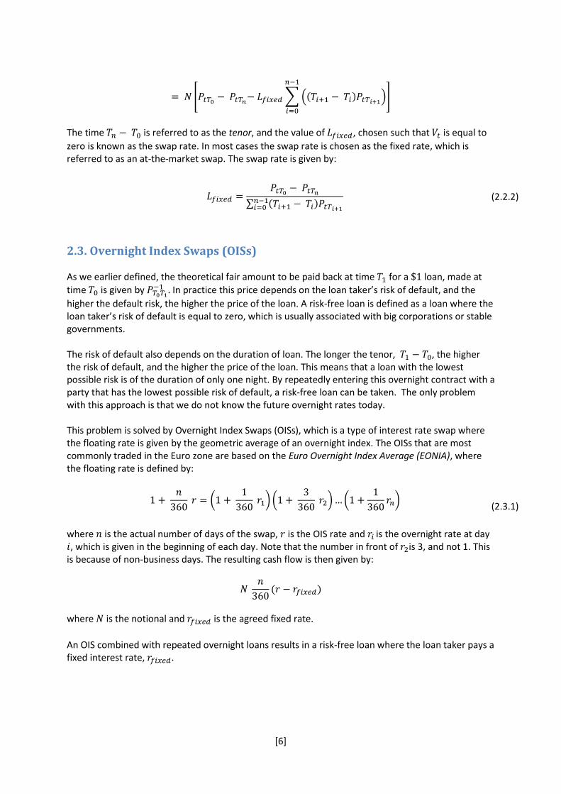
2.3. Overnight Index Swaps (OISs) As we earlier defined, the theoretical fair amount to be paid back at time for a loan, made at
time is given by In practice this price depends on the loan taker’s risk of default, and the
higher the default risk, the higher the price of the loan. A risk-free loan is defined as a loan where the loan taker’s risk of default is equal to zero, which is usually associated with big corporations or stable governments. The risk of default also depends on the duration of loan. The longer the tenor, , the higher the risk of default, and the higher the price of the loan. This means that a loan with the lowest possible risk is of the duration of only one night. By repeatedly entering this overnight contract with a party that has the lowest possible risk of default, a risk-free loan can be taken. The only problem with this approach is that we do not know the future overnight rates today. This problem is solved by Overnight Index Swaps (OISs), which is a type of interest rate swap where the floating rate is given by the geometric average of an overnight index. The OISs that are most commonly traded in the Euro zone are based on the Euro Overnight Index Average (EONIA), where the floating rate is defined by:
(
) (
) (
)
(2.3.1)
where is the actual number of days of the swap, is the OIS rate and is the overnight rate at day , which is given in the beginning of each day. Note that the number in front of is 3, and not 1. This is because of non-business days. The resulting cash flow is then given by:
where is the notional and is the agreed fixed rate.
An OIS combined with repeated overnight loans results in a risk-free loan where the loan taker pays a fixed interest rate, .
[7]
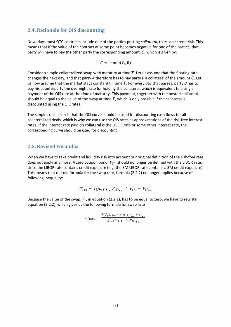
2.4. Rationale for OIS discounting Nowadays most OTC contracts include one of the parties posting collateral, to escape credit risk. This means that if the value of the contract at some point becomes negative for one of the parties, that party will have to pay the other party the corresponding amount, , which is given by:
Consider a simple collateralized swap with maturity at time . Let us assume that the floating rate changes the next day, and that party A therefore has to pay party B a collateral of the amount . Let us now assume that the market stays constant till time . For every day that passes, party B has to pay his counterparty the overnight rate for holding the collateral, which is equivalent to a single payment of the OIS rate at the time of maturity. This payment, together with the posted collateral, should be equal to the value of the swap at time , which is only possible if the collateral is discounted using the OIS rates. The simple conclusion is that the OIS curve should be used for discounting cash flows for all collateralized deals, which is why we can use the OIS rates as approximations of the risk-free interest rates. If the interest rate paid on collateral is the LIBOR rate or some other interest rate, the corresponding curve should be used for discounting.
2.5. Revised Formulas When we have to take credit and liquidity risk into account our original definition of the risk-free rate does not apply any more. A zero coupon bond, , should no longer be defined with the LIBOR rate, since the LIBOR rate contains credit exposure (e.g. the 3M LIBOR rate contains a 3M credit exposure). This means that our old formula for the swap rate, formula (2.2.2) no longer applies because of following inequality:
Because the value of the swap, , in equation (2.2.1), has to be equal to zero, we have to rewrite equation (2.2.2), which gives us the following formula for swap rate
∑
∑
[8]
3. The Model
3.1. Constructing the LIBOR and OIS yield curves
To price and value the illiquid instrument we are analyzing, we need to construct the LIBOR curve to
compute the swap rate and the OIS curve to compute the discount rate.
The LIBOR curve is constructed from a number of different instruments, namely swaps, FRAs, futures
and deposits. For the time points of which we have market data for liquid instruments, the prices will
be exactly reconstructed. We then get a curve, by interpolating between these time points, which we
can use to price and value illiquid instruments (such as a 7½Y swap or a forward starting swap). The
interpolation can be done in a multiple number of ways, where linear interpolation arguably is the
simplest.
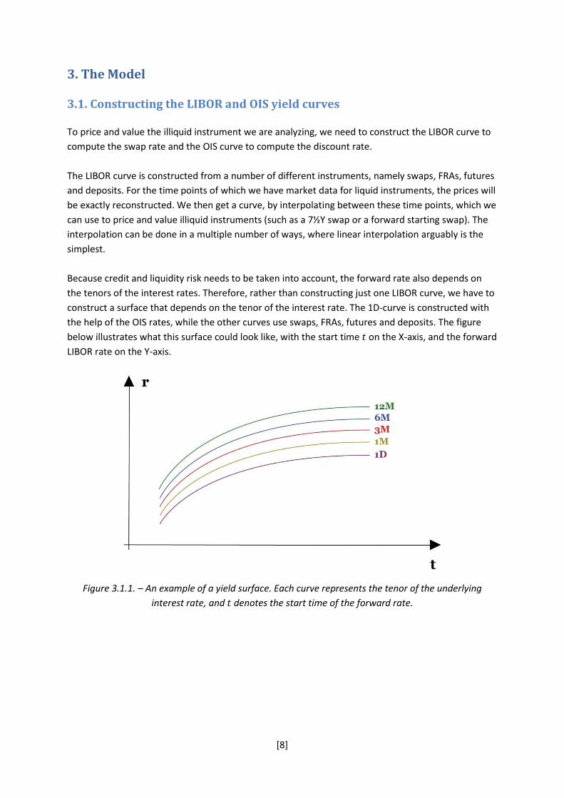
Because credit and liquidity risk needs to be taken into account, the forward rate also depends on
the tenors of the interest rates. Therefore, rather than constructing just one LIBOR curve, we have to
construct a surface that depends on the tenor of the interest rate. The 1D-curve is constructed with
the help of the OIS rates, while the other curves use swaps, FRAs, futures and deposits. The figure
below illustrates what this surface could look like, with the start time on the X-axis, and the forward
LIBOR rate on the Y-axis.
Figure 3.1.1. – An example of a yield surface. Each curve represents the tenor of the underlying
interest rate, and denotes the start time of the forward rate.

[9]
3.2. The Swaps dependence on the OISs
In section 2.2. we defined the present value of a swap as:
∑ (
)
(3.2.1)
Because of the last factor in equation (3.2.1),
, which is dependent on the OIS rates and the
discount time (so we should rather denote it as ), is not a linear function (which is
easily seen from equation (2.3.1)). up to a year is given by the following expression:
where is the OIS rate in the interval [ ]. Note that the expression above is only true for tenors shorter than a year, since the OISs also include yearly payments (which will not matter in our case since our simulations are only over a timespan of one year). We could therefore approximate
with its Taylor expansion:
( )
So a small change in the OIS rate will affect the present value of the swap linearly, but whenever we see large shifts in the OIS curve, the second order of the Taylor expansion takes over and we get a convex dependence. As we have established above, the present value of the swap has a direct dependence on the OIS rates through the discount factor, but because the swap rate of our illiquid instrument, , is dependent on both the LIBOR rates,
, and the OIS rates, , and the LIBOR rates in turn are
built up using the swap rates and the OIS rates, through the 1D-curve, (and could therefore be written as
)2, we also have an indirect dependence from the OIS rates on the present
value through the LIBOR rate.
∑ (
)
(3.2.2)
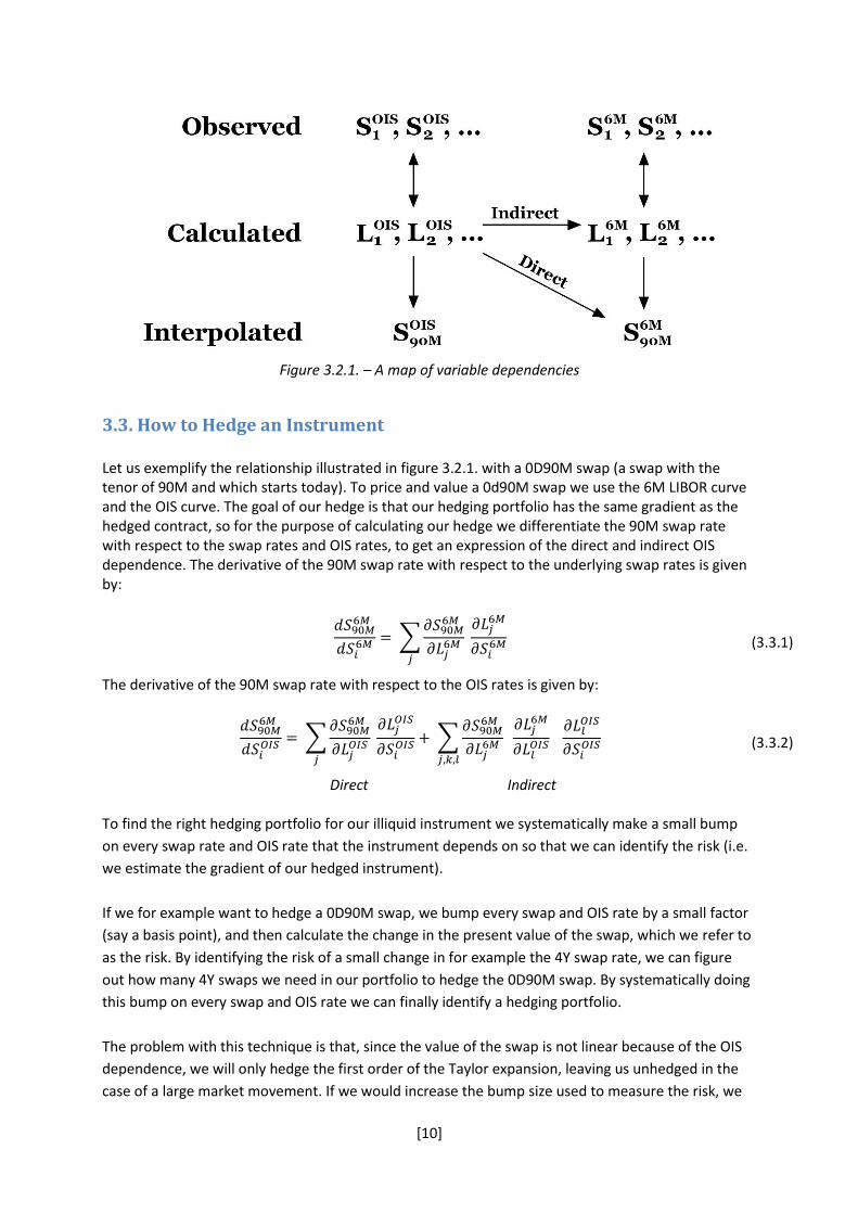
Indirect Direct So the OIS dependence on the value of a swap is indeed quite complex. Figure 3.2.1. below, should make this dependence a little more clear. The analyzed instruments in this project use the 6M LIBOR
curve, and that is why we denote the swap rates as .
2 The OIS dependence on the swap rates are incorporated into the market price for the liquid instruments, but
when we price an illiquid instrument, such as a forward starting swap, we have to take this dependence into account, since it should affects our hedge.
[10]
Figure 3.2.1. – A map of variable dependencies
3.3. How to Hedge an Instrument Let us exemplify the relationship illustrated in figure 3.2.1. with a 0D90M swap (a swap with the tenor of 90M and which starts today). To price and value a 0d90M swap we use the 6M LIBOR curve and the OIS curve. The goal of our hedge is that our hedging portfolio has the same gradient as the hedged contract, so for the purpose of calculating our hedge we differentiate the 90M swap rate with respect to the swap rates and OIS rates, to get an expression of the direct and indirect OIS dependence. The derivative of the 90M swap rate with respect to the underlying swap rates is given by:
∑
(3.3.1)
The derivative of the 90M swap rate with respect to the OIS rates is given by:
∑
∑
(3.3.2)
Direct Indirect To find the right hedging portfolio for our illiquid instrument we systematically make a small bump
on every swap rate and OIS rate that the instrument depends on so that we can identify the risk (i.e.
we estimate the gradient of our hedged instrument).
If we for example want to hedge a 0D90M swap, we bump every swap and OIS rate by a small factor
(say a basis point), and then calculate the change in the present value of the swap, which we refer to
as the risk. By identifying the risk of a small change in for example the 4Y swap rate, we can figure
out how many 4Y swaps we need in our portfolio to hedge the 0D90M swap. By systematically doing
this bump on every swap and OIS rate we can finally identify a hedging portfolio.
The problem with this technique is that, since the value of the swap is not linear because of the OIS
dependence, we will only hedge the first order of the Taylor expansion, leaving us unhedged in the
case of a large market movement. If we would increase the bump size used to measure the risk, we

[11]
would instead be better hedged for larger movements, but worse hedged for smaller movements.
This tradeoff is illustrated in the figure below.
Figure 3.3.2. – The tradeoff between making a small or large bump when calculating the risk
One could possibly try to do these bumps on the OIS rates and the swap rates simultaneously, and in
some way solve an optimization problem which minimizes the total risk, but this would be much
more complex, and lead to a much slower price setting tool.
What we do here is a delta hedge, meaning that we only try to hedge the first order of the Taylor
expansion. An interesting question would be why we only do a delta hedge, and do not try to do a
gamma hedge (which means that we hedge the second order of the Taylor expansion), which is
commonly done for option hedging.
In the case of option hedging we have many more instruments to choose from when we build the
hedging portfolio, since options with different strike prices could be considered as different
instruments. A larger number of instruments would be needed in the hedging portfolio for a gamma
hedge relative to a delta hedge. When we delta hedge an interest rate swap we use as many
instruments as there are constraints (every bump identifies a risk, which has to be covered by an
instrument), which means that there are no instruments left to hedge with if we would like to do a
gamma hedge.
[12]
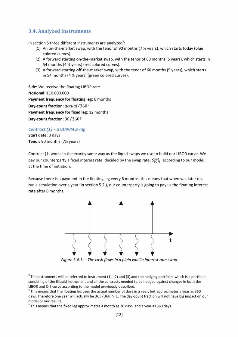
3.4. Analyzed Instruments In section 5 three different instruments are analyzed3:
(1) An on-the-market swap, with the tenor of 90 months (7 ½ years), which starts today (blue colored curves).
(2) A forward starting on-the-market swap, with the tenor of 60 months (5 years), which starts in 54 months (4 ½ years) (red colored curves).
(3) A forward starting off-the-market swap, with the tenor of 60 months (5 years), which starts in 54 months (4 ½ years) (green colored curves).
Side: We receive the floating LIBOR rate
Notional: €10.000.000
Payment frequency for floating leg: 6 months
Day-count fraction: ⁄ 4
Payment frequency for fixed leg: 12 months
Day-count fraction: ⁄ 5
Contract (1) – a 0D90M swap
Start date: 0 days
Tenor: 90 months (7½ years)
Contract (1) works in the exactly same way as the liquid swaps we use to build our LIBOR curve. We
pay our counterparty a fixed interest rate, decided by the swap rate, , according to our model,
at the time of initiation.
Because there is a payment in the floating leg every 6 months, this means that when we, later on,
run a simulation over a year (in section 5.2.), our counterparty is going to pay us the floating interest
rate after 6 months.
Figure 3.4.1. – The cash flows in a plain vanilla interest rate swap
3 The instruments will be referred to instrument (1), (2) and (3) and the hedging portfolio, which is a portfolio
consisting of the illiquid instrument and all the contracts needed to be hedged against changes in both the LIBOR and OIS curve according to the model previously described. 4 This means that the floating leg uses the actual number of days in a year, but approximates a year as 360
days. Therefore one year will actually be ⁄ . The day-count fraction will not have big impact on our model or our results. 5 This means that the fixed leg approximates a month as 30 days, and a year as 360 days.
[13]
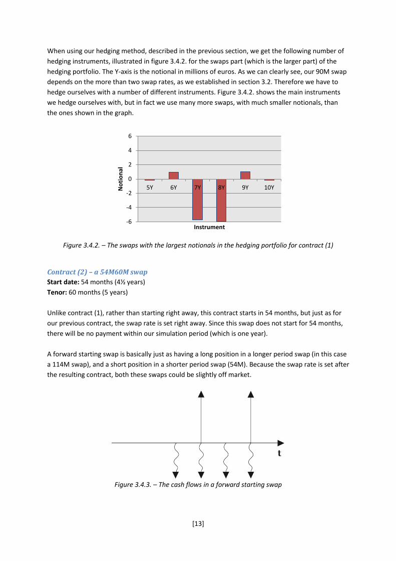
When using our hedging method, described in the previous section, we get the following number of
hedging instruments, illustrated in figure 3.4.2. for the swaps part (which is the larger part) of the
hedging portfolio. The Y-axis is the notional in millions of euros. As we can clearly see, our 90M swap
depends on the more than two swap rates, as we established in section 3.2. Therefore we have to
hedge ourselves with a number of different instruments. Figure 3.4.2. shows the main instruments
we hedge ourselves with, but in fact we use many more swaps, with much smaller notionals, than
the ones shown in the graph.
Figure 3.4.2. – The swaps with the largest notionals in the hedging portfolio for contract (1)
Contract (2) – a 54M60M swap
Start date: 54 months (4½ years)
Tenor: 60 months (5 years)
Unlike contract (1), rather than starting right away, this contract starts in 54 months, but just as for
our previous contract, the swap rate is set right away. Since this swap does not start for 54 months,
there will be no payment within our simulation period (which is one year).
A forward starting swap is basically just as having a long position in a longer period swap (in this case
a 114M swap), and a short position in a shorter period swap (54M). Because the swap rate is set after
the resulting contract, both these swaps could be slightly off market.
Figure 3.4.3. – The cash flows in a forward starting swap
-6
-4
-2
0
2
4
6
5Y 6Y 7Y 8Y 9Y 10YNo
tio
nal
Instrument

[14]
The fact that this contract is the difference between two swaps can be seen from the hedged
portfolio. Because this contract is further away in time than contract (1), it is going to be more
effected by changes in the OIS rates, since we have to discount cash flows further away in time.
Figure 3.4.4. – The notionals for the main hedging swaps for contracts (2) and (3)
Contract (3) – an off-market 54M60M swap
Start date: 54 months (4½ years)
Tenor: 60 months (5 years)
Off-Market rate: 1 %
Contract three is just like contract (2), except for the fact that we have set the fixed rate off-market
to 1 %. This means that we do not calculate the swap rate when we enter the contract. Instead we
just set the fixed rate to 1 %. The big difference from contract (2) is that this contract is equivalent to
having contract (2) with an extra fixed leg. This means that contract (3) is going to depend on the OIS
rates even more, since there are more cash flows to discount.
Figure 3.4.5. – The cash flows for an off market forward starting swap are just like a usual forward
starting swap (i.e. the cash flows start later in time, rather than at day 0), but with an extra fixed leg.
-6
-4
-2
0
2
4
6
3Y 4Y 5Y 6Y 7Y 8Y 9Y 10Y 11YNo
tio
nal
Instruments
[15]
The hedging weights for the swaps, in the hedging portfolio, are going to be exactly the same as for
contract (2), since the dependence on the swap rates is equivalent. On the other hand the OIS hedge
will to be way larger since this contract has a much greater dependence on the OIS rates.
[16]
4. Data
The data used for the simulations in this project is ICAP data, retrieved using Reuters. We only use
the 6M curve in this project, since this is the most liquid one, and therefore the instruments used for
these simulations are the OISs, FRAs, the 6M deposit and swaps. The OIS rates are used to construct
the 1D curve, and the three latter are used to construct the 6M curve. The OIS rates used are the
EONIA rates (Euro Overnight Index Average), and the forward interest rate curve constructed during
this project uses the EURIBOR swap rates (Euro Interbank Offered Rate). Throughout this report we
will denote the EURIBOR rate as the LIBOR rate to avoid any confusion, since this is a term more
frequently used in academic papers.
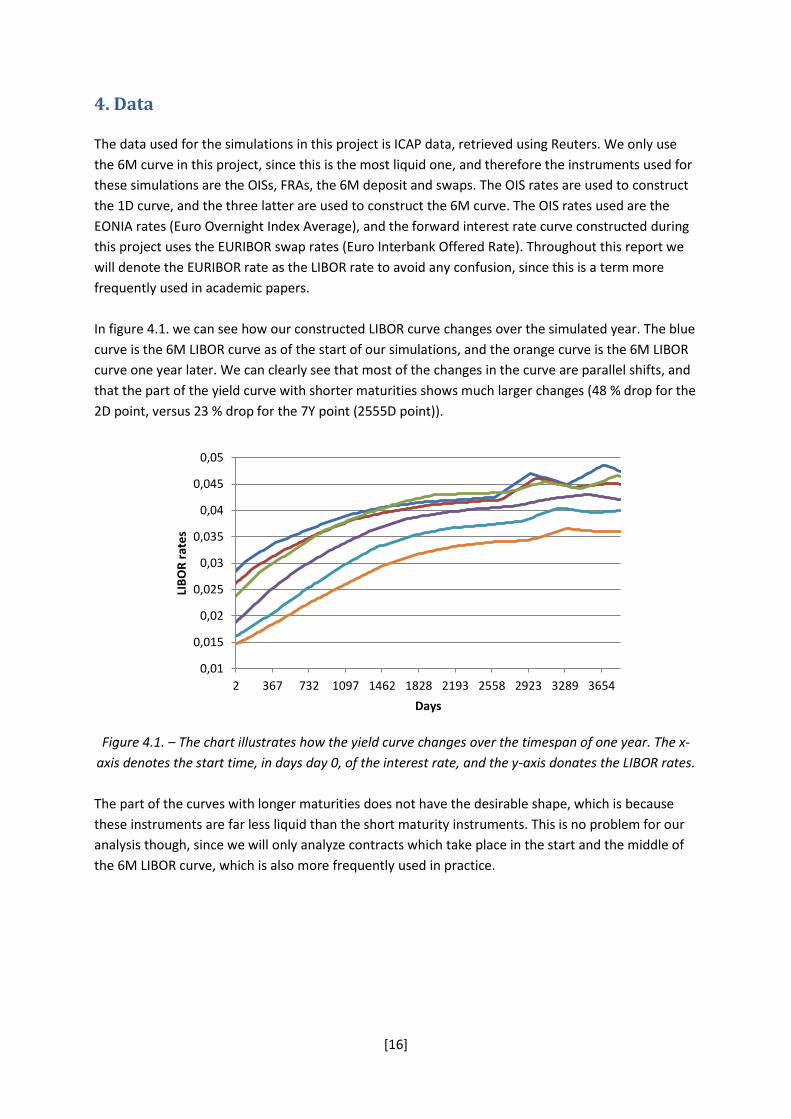
In figure 4.1. we can see how our constructed LIBOR curve changes over the simulated year. The blue
curve is the 6M LIBOR curve as of the start of our simulations, and the orange curve is the 6M LIBOR
curve one year later. We can clearly see that most of the changes in the curve are parallel shifts, and
that the part of the yield curve with shorter maturities shows much larger changes (48 % drop for the
2D point, versus 23 % drop for the 7Y point (2555D point)).
Figure 4.1. – The chart illustrates how the yield curve changes over the timespan of one year. The x-
axis denotes the start time, in days day 0, of the interest rate, and the y-axis donates the LIBOR rates.
The part of the curves with longer maturities does not have the desirable shape, which is because
these instruments are far less liquid than the short maturity instruments. This is no problem for our
analysis though, since we will only analyze contracts which take place in the start and the middle of
the 6M LIBOR curve, which is also more frequently used in practice.
0,01
0,015
0,02
0,025
0,03
0,035
0,04
0,045
0,05
2 367 732 1097 1462 1828 2193 2558 2923 3289 3654
LIB
OR
rat
es
Days

[17]
5. Results In this section we will present the results of the run simulations. The blue colored curves will always
represent the 90M swap, the red colored curve the forward starting 54M60M swap and the green
curve the off market 54M60M swap. Whenever we have two y-axes, the 90M swap is shown on the
left y-axis, while the forward starting contracts are shown on the right y-axis.
5.1. Intraday We first test the model by running the simulation intraday, meaning that we are using historical data for up to a year, but never change the dates in the model. So when the interest rates change we measure the present value of the swap as if no time has passed. This implies two things. Firstly, because we will always compare each simulated day with our initial data, it means that the changes in the interest rates will be getting larger with every iterated day (for each iteration we will use a new days data, but as stated above, we never change the dates in the model), since the changes in the swap and OIS rates are going to be aggregated. Secondly, this means that we should be very well hedged, because of the nature of our hedge. As explained in section 3.3., we identify our hedging portfolio by making a separate bump on every interest rate that our illiquid contract depends on. Because this is done without changing any dates, we should see a hedging portfolio with very small changes.
[18]
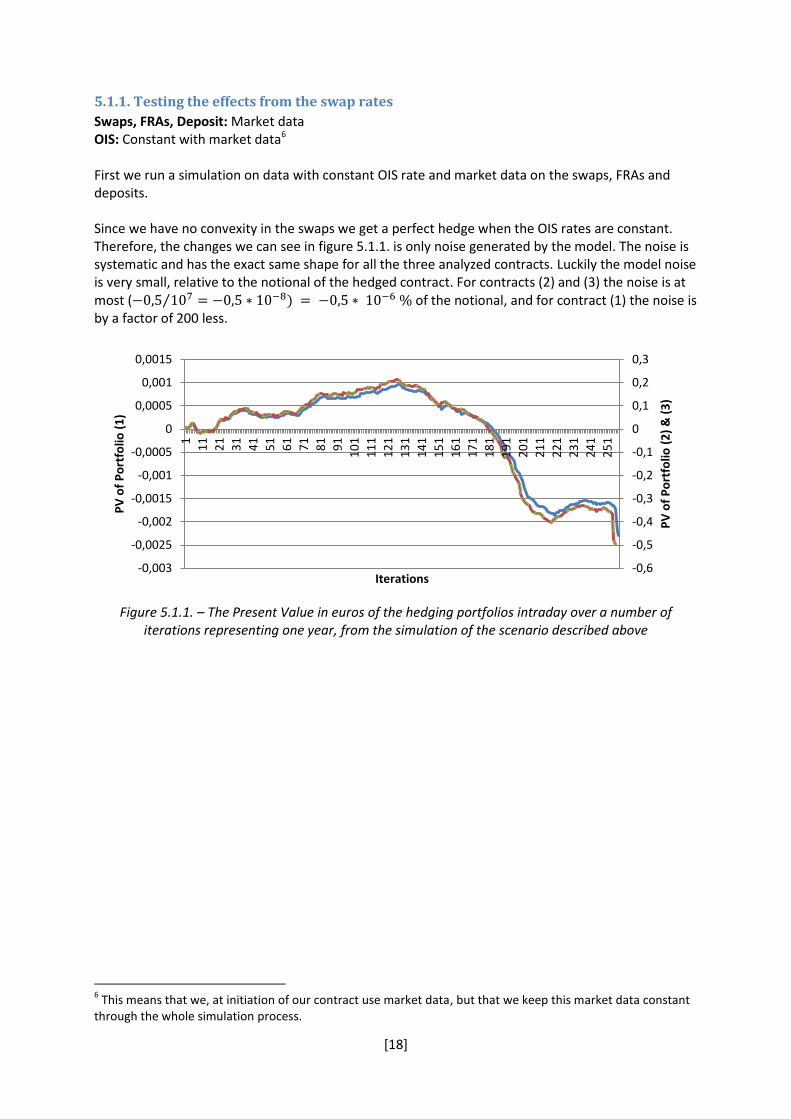
5.1.1. Testing the effects from the swap rates
Swaps, FRAs, Deposit: Market data OIS: Constant with market data6 First we run a simulation on data with constant OIS rate and market data on the swaps, FRAs and deposits. Since we have no convexity in the swaps we get a perfect hedge when the OIS rates are constant. Therefore, the changes we can see in figure 5.1.1. is only noise generated by the model. The noise is systematic and has the exact same shape for all the three analyzed contracts. Luckily the model noise is very small, relative to the notional of the hedged contract. For contracts (2) and (3) the noise is at most ( ⁄ of the notional, and for contract (1) the noise is by a factor of 200 less.
Figure 5.1.1. – The Present Value in euros of the hedging portfolios intraday over a number of
iterations representing one year, from the simulation of the scenario described above
6 This means that we, at initiation of our contract use market data, but that we keep this market data constant
through the whole simulation process.
-0,6
-0,5
-0,4
-0,3
-0,2
-0,1
0
0,1
0,2
0,3
-0,003
-0,0025
-0,002
-0,0015
-0,001
-0,0005
0
0,0005
0,001
0,0015
1
11
21
31
41
51
61
71
81
91
10
1
11
1
12
1
13
1
14
1
15
1
16
1
17
1
18
1
19
1
20
1
21
1
22
1
23
1
24
1
25
1
PV
of
Po
rtfo
lio (
2)
& (
3)
PV
of
Po
rtfo
lio (
1)
Iterations

[19]
5.1.2. Testing the effects from the OIS rates
Swaps, FRAs, Deposit: Constant with market data OIS: Market Data The next step is to figure out the effects of the OIS rates on the hedged portfolio. When the OIS rates are no longer constant we will no longer be perfectly hedged, since we have only been able to hedge ourselves in regard to the first degree in the Taylor expansion. As can be seen in figure 5.1.2. the effects on the portfolio from the OIS rates become much stronger with increasing OIS rates since we have only hedged ourselves for small movements in the OIS curve (see section 3.3.). We also see that portfolios (2) and (3) are more affected by the convexity of the OISs, since they are more dependent on the OIS rates because of cash flows further away in time. The reason we see slightly larger movements in portfolio (3), compared to portfolio (2), is because the OIS rates also affect the fixed leg of an off-market contract. We can still note that the deviation from zero, of the present value, is still very small, in relation to the notional of the hedged contract.
Figure 5.1.2. – The Present Value in euros of the hedging portfolios intraday over a number of
iterations representing one year, from the simulation of the scenario described above
-0,5
0
0,5
1
1,5
2
-0,1
-0,05
0
0,05
0,1
0,15
0,2
0,25
0,3
0,35
0,4
1
11
21
31
41
51
61
71
81
91
10
1
11
1
12
1
13
1
14
1
15
1
16
1
17
1
18
1
19
1
20
1
21
1
22
1
23
1
24
1
25
1
PV
of
Po
rtfo
lios
(2)
& (
3)
PV
of
Po
rtfo
lio (
1)
Iterations
[20]
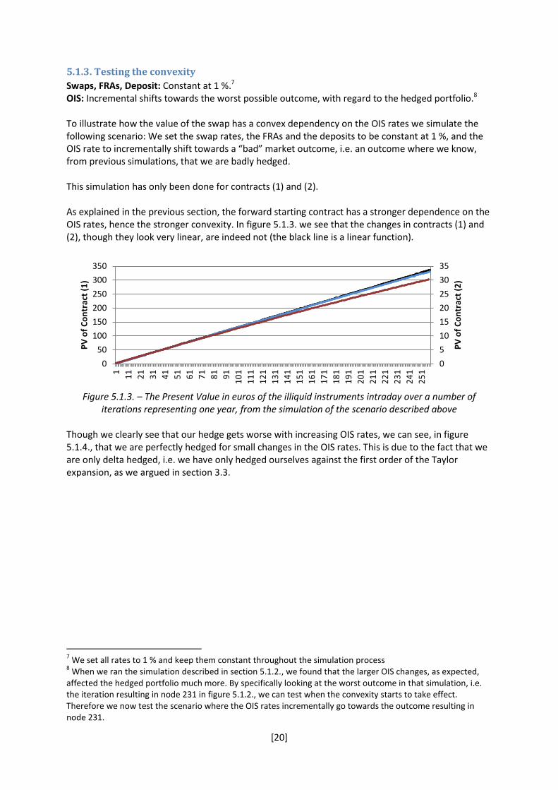
5.1.3. Testing the convexity
Swaps, FRAs, Deposit: Constant at 1 %.7 OIS: Incremental shifts towards the worst possible outcome, with regard to the hedged portfolio.8 To illustrate how the value of the swap has a convex dependency on the OIS rates we simulate the following scenario: We set the swap rates, the FRAs and the deposits to be constant at 1 %, and the OIS rate to incrementally shift towards a “bad” market outcome, i.e. an outcome where we know, from previous simulations, that we are badly hedged. This simulation has only been done for contracts (1) and (2). As explained in the previous section, the forward starting contract has a stronger dependence on the OIS rates, hence the stronger convexity. In figure 5.1.3. we see that the changes in contracts (1) and (2), though they look very linear, are indeed not (the black line is a linear function).
Figure 5.1.3. – The Present Value in euros of the illiquid instruments intraday over a number of
iterations representing one year, from the simulation of the scenario described above Though we clearly see that our hedge gets worse with increasing OIS rates, we can see, in figure 5.1.4., that we are perfectly hedged for small changes in the OIS rates. This is due to the fact that we are only delta hedged, i.e. we have only hedged ourselves against the first order of the Taylor expansion, as we argued in section 3.3.
7 We set all rates to 1 % and keep them constant throughout the simulation process
8 When we ran the simulation described in section 5.1.2., we found that the larger OIS changes, as expected,
affected the hedged portfolio much more. By specifically looking at the worst outcome in that simulation, i.e. the iteration resulting in node 231 in figure 5.1.2., we can test when the convexity starts to take effect. Therefore we now test the scenario where the OIS rates incrementally go towards the outcome resulting in node 231.
0
5
10
15
20
25
30
35
0
50
100
150
200
250
300
350
1
11
21
31
41
51
61
71
81
91
10
1
11
1
12
1
13
1
14
1
15
1
16
1
17
1
18
1
19
1
20
1
21
1
22
1
23
1
24
1
25
1
PV
of
Co
ntr
act
(2)
PV
of
Co
ntr
act
(1)

[21]
Figure 5.1.4. – The Present Value in euros of the hedging portfolios intraday over a number of
iterations representing, from the simulation of the scenario described above
5.1.4. Running the simulation
Swaps, FRAs, Deposit: Market data OIS: Market data
Finally we run a simulation where we use market data for all instruments, which generates a quite
surprising result. As we can see from figure 5.1.5., the loss has increased with a factor of 20-50
compared to the results we got when we used fixed data on the swaps. One might have thought that
the loss in this case would have been the sum of the losses for controlling for swaps and OISs, but
here we see a much worse outcome (though still pretty acceptable relative to the notional of the
contract).
Figure 5.1.5. – The Present Value in euros of the hedging portfolios intraday over a number of
iterations representing one year, from the simulation of the scenario described above
Recall what we discussed in section 3.2. regarding how the contract value depends on the OIS rates.
We established that the present value of the illiquid instrument depends on both the swap rates and
the OIS rates, and thereafter we derived its Taylor expansion. But because the present value is
dependent on both the swap rates and the OIS rates we can differentiate as follows:
-1,4
-1,2
-1
-0,8
-0,6
-0,4
-0,2
0
-0,07
-0,06
-0,05
-0,04
-0,03
-0,02
-0,01
0
1
11
21
31
41
51
61
71
81
91
10
1
11
1
12
1
13
1
14
1
15
1
16
1
17
1
18
1
19
1
20
1
21
1
22
1
23
1
24
1
25
1
PV
of
Po
rtfo
lio (
2)
PV
of
Po
rtfo
lio (
1)
Iterations
-20
0
20
40
60
80
100
-2
0
2
4
6
8
10
1
11
21
31
41
51
61
71
81
91
10
1
11
1
12
1
13
1
14
1
15
1
16
1
17
1
18
1
19
1
20
1
21
1
22
1
23
1
24
1
25
1
PV
of
Po
rtfo
lio (
2)
& (
3)
PV
of
Po
rtfo
lio (
1)
Iterations
[22]
( ) ∑
∑
∑∑
∑∑
∑∑
(
)
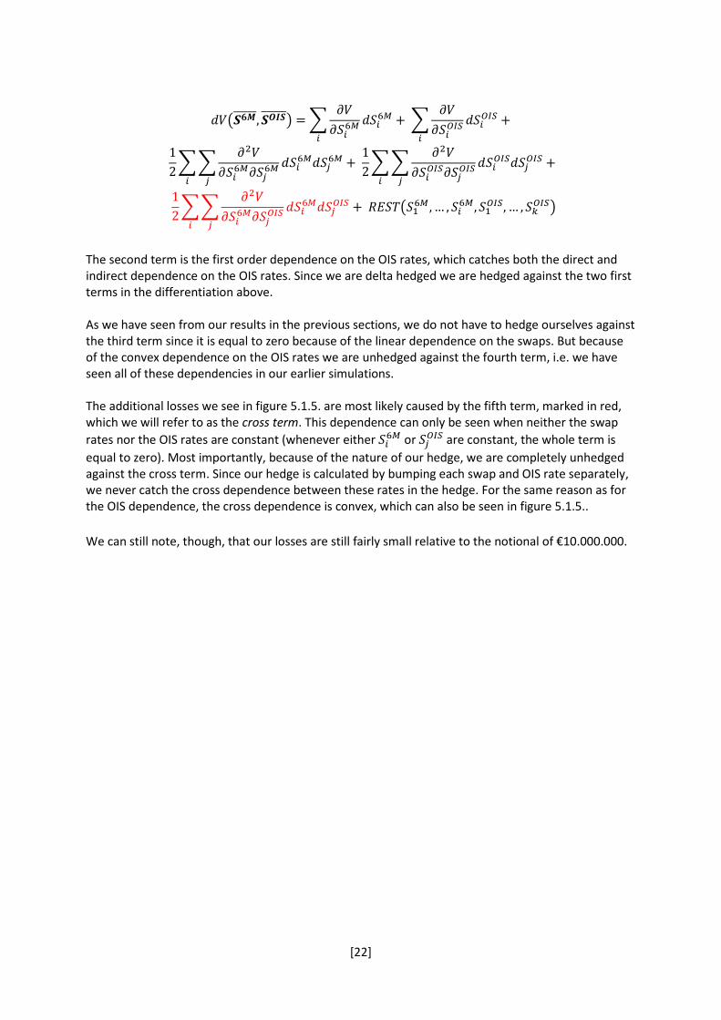
The second term is the first order dependence on the OIS rates, which catches both the direct and indirect dependence on the OIS rates. Since we are delta hedged we are hedged against the two first terms in the differentiation above. As we have seen from our results in the previous sections, we do not have to hedge ourselves against the third term since it is equal to zero because of the linear dependence on the swaps. But because of the convex dependence on the OIS rates we are unhedged against the fourth term, i.e. we have seen all of these dependencies in our earlier simulations. The additional losses we see in figure 5.1.5. are most likely caused by the fifth term, marked in red, which we will refer to as the cross term. This dependence can only be seen when neither the swap
rates nor the OIS rates are constant (whenever either or
are constant, the whole term is
equal to zero). Most importantly, because of the nature of our hedge, we are completely unhedged against the cross term. Since our hedge is calculated by bumping each swap and OIS rate separately, we never catch the cross dependence between these rates in the hedge. For the same reason as for the OIS dependence, the cross dependence is convex, which can also be seen in figure 5.1.5..
We can still note, though, that our losses are still fairly small relative to the notional of €10.000.000.
[23]
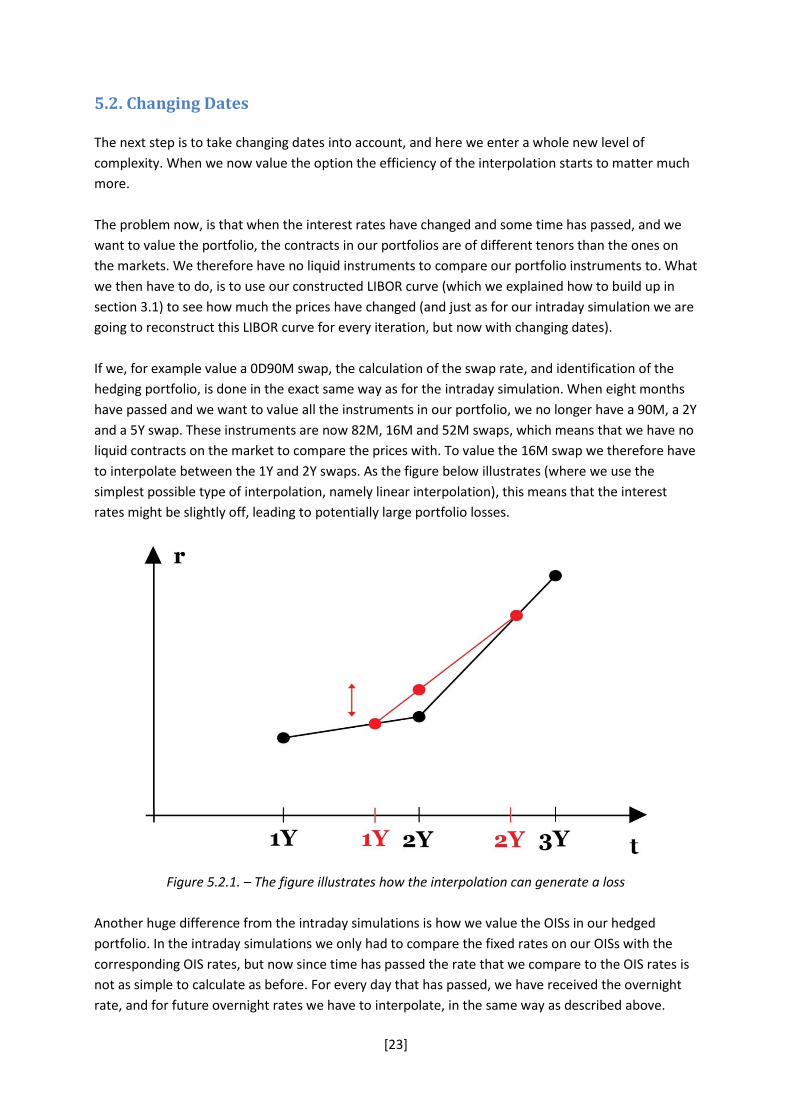
5.2. Changing Dates
The next step is to take changing dates into account, and here we enter a whole new level of
complexity. When we now value the option the efficiency of the interpolation starts to matter much
more.
The problem now, is that when the interest rates have changed and some time has passed, and we
want to value the portfolio, the contracts in our portfolios are of different tenors than the ones on
the markets. We therefore have no liquid instruments to compare our portfolio instruments to. What
we then have to do, is to use our constructed LIBOR curve (which we explained how to build up in
section 3.1) to see how much the prices have changed (and just as for our intraday simulation we are
going to reconstruct this LIBOR curve for every iteration, but now with changing dates).
If we, for example value a 0D90M swap, the calculation of the swap rate, and identification of the
hedging portfolio, is done in the exact same way as for the intraday simulation. When eight months
have passed and we want to value all the instruments in our portfolio, we no longer have a 90M, a 2Y
and a 5Y swap. These instruments are now 82M, 16M and 52M swaps, which means that we have no
liquid contracts on the market to compare the prices with. To value the 16M swap we therefore have
to interpolate between the 1Y and 2Y swaps. As the figure below illustrates (where we use the
simplest possible type of interpolation, namely linear interpolation), this means that the interest
rates might be slightly off, leading to potentially large portfolio losses.
Figure 5.2.1. – The figure illustrates how the interpolation can generate a loss
Another huge difference from the intraday simulations is how we value the OISs in our hedged
portfolio. In the intraday simulations we only had to compare the fixed rates on our OISs with the
corresponding OIS rates, but now since time has passed the rate that we compare to the OIS rates is
not as simple to calculate as before. For every day that has passed, we have received the overnight
rate, and for future overnight rates we have to interpolate, in the same way as described above.

[24]
Let us ones again exemplify. If four months have passed this means that we have received the
overnight rate every business day for four months. To value a 2Y OIS in our hedged portfolio (which
now only is a 20M OIS) we first use the four months of given overnight rates, and for the remaining
20M we interpolate between todays 1Y and 2Y OIS. We finally get the following expression for the
“floating” OIS rate:
∏(
)(
)
where N is the numbers of days left (in this example approximately 600 days), x in this example is 20,
and
is the overnight rate for day (TN stands for “Tomorrow Next”). To get the present value of
the OIS we compare this rate with the fixed rate, which was decided by the OIS rate at time .
Figure 5.2.2. – The figure illustrates the cash flows we use when calculating the OIS rate in a “living”
contract.

[25]
5.2.1. Testing for all Variables Constant
Swaps, FRAs, Deposit: Constant with market data OIS: Constant with market data
In the simplest case we keep all rates constant, and try to figure out how the change in dates affects
the value of the portfolio.
Figure 5.2.3. – The Present Value in euros of the illiquid instruments over a time span of one year,
from the simulation of the scenario described above
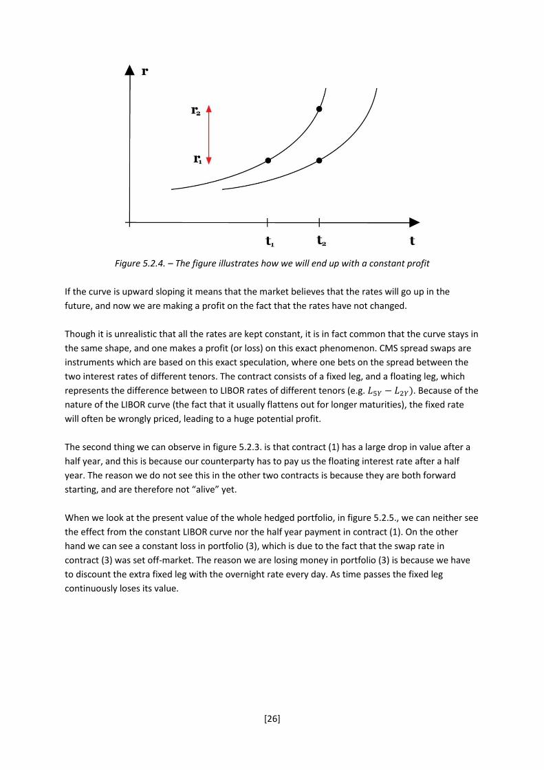
The first thing we can observe is that all three contracts constantly increase in value. At first glance
this might seem strange, since neither the swap rates nor the OIS rates are changing, but because of
the shape of the LIBOR curve this actually makes sense. Let us elaborate.
When one year has passed, our 2Y swaps are now 1Y swaps, but the LIBOR curve looks exactly the
same as it did one year ago. The fixed rate of that swap was set one year ago, and to the 2Y swap
rate, but now we are comparing this swap rate to the 1Y rate, which is the same as the 1Y rate was
one year ago and therefore much lower. This leads to an arbitrage opportunity, since the fact that
the curve is kept constant means we always make money.
020000400006000080000
100000120000140000160000180000200000
PV
of
Co
ntr
acts
(1
), (
2)
& (
3)
Days
[26]
Figure 5.2.4. – The figure illustrates how we will end up with a constant profit
If the curve is upward sloping it means that the market believes that the rates will go up in the
future, and now we are making a profit on the fact that the rates have not changed.
Though it is unrealistic that all the rates are kept constant, it is in fact common that the curve stays in
the same shape, and one makes a profit (or loss) on this exact phenomenon. CMS spread swaps are
instruments which are based on this exact speculation, where one bets on the spread between the
two interest rates of different tenors. The contract consists of a fixed leg, and a floating leg, which
represents the difference between to LIBOR rates of different tenors (e.g. . Because of the
nature of the LIBOR curve (the fact that it usually flattens out for longer maturities), the fixed rate
will often be wrongly priced, leading to a huge potential profit.
The second thing we can observe in figure 5.2.3. is that contract (1) has a large drop in value after a
half year, and this is because our counterparty has to pay us the floating interest rate after a half
year. The reason we do not see this in the other two contracts is because they are both forward
starting, and are therefore not “alive” yet.
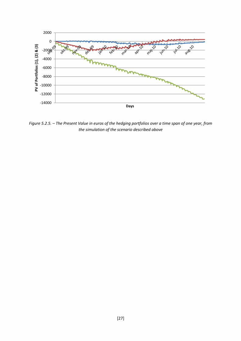
When we look at the present value of the whole hedged portfolio, in figure 5.2.5., we can neither see
the effect from the constant LIBOR curve nor the half year payment in contract (1). On the other
hand we can see a constant loss in portfolio (3), which is due to the fact that the swap rate in
contract (3) was set off-market. The reason we are losing money in portfolio (3) is because we have
to discount the extra fixed leg with the overnight rate every day. As time passes the fixed leg
continuously loses its value.
[27]
Figure 5.2.5. – The Present Value in euros of the hedging portfolios over a time span of one year, from
the simulation of the scenario described above
-14000
-12000
-10000
-8000
-6000
-4000
-2000
0
2000P
V o
f P
ort
folio
s (1
), (
2)
& (
3)
Days

[28]
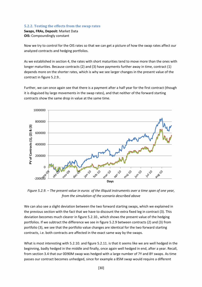
Swaps, FRAs, Deposit: Constant at 1 % OIS: Compoundingly constant9
So if we set the swap rates to be constant at 1 %, we should no longer see the LIBOR spread effect
(the effect that could be associated to the CMS spread swaps). We also set our OIS rates to
“compoundingly constant”, so that we do not make an arbitrage profit.
Just as in the previous simulation we see a constant loss in contact (3) because of the discounting of
the extra fixed leg, but for the other two contracts, we indeed see a much smaller value change.
Figure 5.2.6. – The Present Value in euros of the illiquid instruments over a time span of one year,
from the simulation of the scenario described above
The reason we still see changes in contracts (1) and (2), and the reason we are still not perfectly
hedged for the corresponding portfolios is that though we have set all swap rates equal to 1 %, our
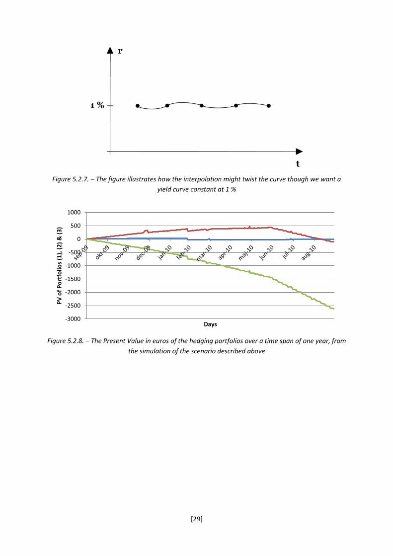
LIBOR curve is still not constant at 1 % because of the interpolation method being used (see figure
5.2.7.). This will have a quite big impact on the whole portfolio since we have to interpolate the rates
for all contracts in the portfolio, every day. For this reason we can observe quite large deviations
from 1 % (up to 15 basis points), which could be regarded as a model error.
9 This means that we set our overnight rate to constant at 1 %, and every OIS rate to the daily compounded
value of the overnight rate, e.g. the 1Y OIS rate is set so that it is equal to the compounded rate given if you receive the overnight rate at 1 % for a year. The reason we cannot set all the OIS rates to 1 % is that we will make a constant arbitrage profit since the overnight rate at 1 % compounded for a year would be larger than 1 %.
-3500
-3000
-2500
-2000
-1500
-1000
-500
0
500
PV
of
Co
ntr
acts
(1
), (
2)
& (
3)
[29]
Figure 5.2.7. – The figure illustrates how the interpolation might twist the curve though we want a
yield curve constant at 1 %
Figure 5.2.8. – The Present Value in euros of the hedging portfolios over a time span of one year, from
the simulation of the scenario described above
-3000
-2500
-2000
-1500
-1000
-500
0
500
1000
PV
of
Po
rtfo
lios
(1),
(2
) &
(3
)
Days
[30]
5.2.2. Testing the effects from the swap rates
Swaps, FRAs, Deposit: Market Data OIS: Compoundingly constant
Now we try to control for the OIS rates so that we can get a picture of how the swap rates affect our
analyzed contracts and hedging portfolios.
As we established in section 4, the rates with short maturities tend to move more than the ones with
longer maturities. Because contracts (2) and (3) have payments further away in time, contract (1)
depends more on the shorter rates, which is why we see larger changes in the present value of the
contract in figure 5.2.9..
Further, we can once again see that there is a payment after a half year for the first contract (though
it is disguised by large movements in the swap rates), and that neither of the forward starting
contracts show the same drop in value at the same time.
Figure 5.2.9. – The present value in euros of the illiquid instruments over a time span of one year,
from the simulation of the scenario described above
We can also see a slight deviation between the two forward starting swaps, which we explained in
the previous section with the fact that we have to discount the extra fixed leg in contract (3). This
deviation becomes much clearer in figure 5.2.10., which shows the present value of the hedging
portfolios. If we subtract the difference we see in figure 5.2.9 between contracts (2) and (3) from
portfolio (3), we see that the portfolio value changes are identical for the two forward starting
contracts, i.e. both contracts are affected in the exact same way by the swaps.
What is most interesting with 5.2.10. and figure 5.2.11. is that it seems like we are well hedged in the
beginning, badly hedged in the middle and finally, once again well hedged in end, after a year. Recall,
from section 3.4 that our 0D90M swap was hedged with a large number of 7Y and 8Y swaps. As time
passes our contract becomes unhedged, since for example a 85M swap would require a different
-200000
0
200000
400000
600000
800000
1000000
PV
of
Co
ntr
acts
(1
), (
2)
& (
3)
Days
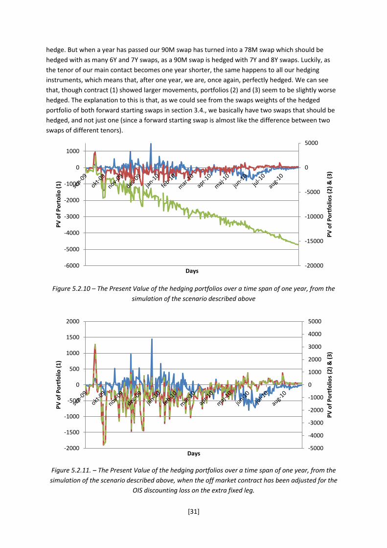
[31]
hedge. But when a year has passed our 90M swap has turned into a 78M swap which should be
hedged with as many 6Y and 7Y swaps, as a 90M swap is hedged with 7Y and 8Y swaps. Luckily, as
the tenor of our main contact becomes one year shorter, the same happens to all our hedging
instruments, which means that, after one year, we are, once again, perfectly hedged. We can see
that, though contract (1) showed larger movements, portfolios (2) and (3) seem to be slightly worse
hedged. The explanation to this is that, as we could see from the swaps weights of the hedged
portfolio of both forward starting swaps in section 3.4., we basically have two swaps that should be
hedged, and not just one (since a forward starting swap is almost like the difference between two
swaps of different tenors).
Figure 5.2.10 – The Present Value of the hedging portfolios over a time span of one year, from the
simulation of the scenario described above
Figure 5.2.11. – The Present Value of the hedging portfolios over a time span of one year, from the
simulation of the scenario described above, when the off market contract has been adjusted for the
OIS discounting loss on the extra fixed leg.
-20000
-15000
-10000
-5000
0
5000
-6000
-5000
-4000
-3000
-2000
-1000
0
1000
PV
of
Po
rtfo
lios
(2)
& (
3)
PV
of
Po
rto
lio (
1)
Days
-5000
-4000
-3000
-2000
-1000
0
1000
2000
3000
4000
5000
-2000
-1500
-1000
-500
0
500
1000
1500
2000P
V o
f P
ort
folio
s (2
) &
(3
)
PV
of
Po
rtfo
lio (
1)
Days

[32]
The reason the portfolio value is not exactly zero after a year has to do with a modeling error, due to
the nature of the hedging model and the interpolation we are using. As we could see in section 3.4.,
the contracts were hedged symmetrically with “surrounding” swaps (i.e. a 90M swap was hedged
with approximately 0,6 7Y and 8Y swaps, -0,1 6Y and 9Y swaps, and so on). So when there are no
“surrounding” instruments to hedge with, the hedged portfolio will be slightly off (e.g. if we would
try to hedge a 46M swap we would, according to the model, need 0,6 3Y and 4Y swaps, -0,1 2Y and
5Y swaps, but since there is no liquid 2Y swap on the market, and this part of the LIBOR curved is
actually built up by FRAs, our hedge would be slightly off, because of inconsistencies in the
instruments). The fact that we actually ended up quite close to zero was pure luck, since we
unknowingly managed to choose a contract with many “surrounding” liquid instruments.
To see for which contracts the swap hedge will be perfect after one year, we run a simulation, with
constant OIS rates and market data for the swap rates, for ten contracts of different tenors (not
forward starting). As we described above, we should be well hedged for the contracts with many
“surrounding” liquid swaps, i.e. the ones with tenors in the middle of the LIBOR curve, and we can
clearly see, in figure 5.2.12., which shows the portfolio loss after one year for the different illiquid
instruments, that this is actually the case. The 30M and 42M swaps are too close to the FRA-part of
the LIBOR-curve, while the contracts further away on the curve are less liquid and can therefore not
be used when building up the LIBOR curve (e.g. the 16Y or 23Y swaps).
Figure 5.2.12 – The chart illustrates that the contracts with many “surrounding” liquid instruments
give a better swap hedge. The x-axis shows a number of instruments of different maturities, and the
y-axis show the present value in euros of the hedging portfolio after one year.
0
100
200
300
400
500
600
700
800
2½Y 3½Y 4½Y 5½Y 6½Y 7½Y 8½Y 9½Y 10½Y 11½Y
The
PV
aft
er
1Y
Swaps

[33]
5.2.3. Testing the effects from the OIS rates
Swaps, FRAs, Deposit: Constant OIS: Market Data
Just as for the intraday simulations we now test the effects of the OIS rates by setting the swap rates
to constant. The reason we do not set all swap rates to 1 % is that we want a more realistic situation,
which leads to a similar situation as in section 5.2.1., where we make a profit as if we had invested in
a CMS spread swap. Rather than looking at the actual change in the value of the contracts and
portfolios, we should look at how the OIS rates affect the contracts and portfolios. We do this by
running the simulation as usual, which results in the left graphs in figures 5.2.13. and 5.2.14. We then
subtract the results we got in section 5.2.1., and this way only see the OIS effect, which is shown in
the right parts of figures 5.2.13. and 5.2.14..
Figure 5.2.13 – The Present Value in euros of the illiquid instruments over a time span of one year,
from the simulation of the scenario described above (the right chart is adjusted to not include the
profit given by the spread between the interest rates).
Just as expected, both forward starting contracts are much more dependent on the OIS rates since
they have more cash flows further away in time, which we see in the right graph of Figure 5.2.13.. A
large part of this OIS dependence is also due to the fact that the forward starting contracts consist of
two, slightly off market, today starting swaps, which means that we have two extra fixed legs that
have to be discounted. We can also see that the off-market swap is much more dependent on the
OIS rate because of its extra fixed leg. The loss that is generated due to the daily discounting of the
extra fixed leg, which we also saw in section 5.2.1. is eliminated, and we only see the effects of
changing OIS rates.
-100000
-50000
0
50000
100000
150000
200000
250000
PV
of
Co
ntr
acts
(1
), (
2)
& (
3)
Days -100000
-80000
-60000
-40000
-20000
0
20000
40000
PV
of
Co
ntr
acts
(1
), (
2)
& (
3)
Days
[34]
The portfolio effects are illustrated in the graphs below, and we can see similar effects as for the
single contracts.
Figure 5.2.14 – The Present Value in euros of the hedging portfolios over a time span of one year,
from the simulation of the scenario described above (the right chart is adjusted to not include the
profit given by the spread between the interest rates).
-25000
-20000
-15000
-10000
-5000
0
5000se
p-0
9
okt
-09
no
v-0
9
dec
-09
jan
-10
feb
-10
mar
-10
apr-
10
maj
-10
jun
-10
jul-
10
aug-
10
PV
of
Po
rtfo
lios
(1),
(2
) &
(3
)
Days -10000
-8000
-6000
-4000
-2000
0
2000
4000
sep
-09
okt
-09
no
v-0
9
dec
-09
jan
-10
feb
-10
mar
-10
apr-
10
maj
-10
jun
-10
jul-
10
aug-
10
PV
of
Po
rto
flio
s (1
), (
2)
& (
3)
Days

[35]
5.2.4. Running the simulation
Swaps, FRAs, Deposit: Market Data OIS: Market Data
Finally it is time to run the most realistic simulation, namely the one using market data for all
instruments, and where the dates are changing.
Most of the changes we see in the contacts and the portfolios are already explained in previous
sections, so let us therefore summarize what could be said about the results below.
- The 0D90M swap is more affected by the swap rates with shorter maturities, which are the
ones which tend to change the most. This explains why contract (1) changes more than the
others (explained in section 5.2.2.)
- The two forward starting contracts are more affected by changes in the OIS curve.
- After a half year we can see a drop in the value of contract (1) since it is “alive”. This cannot
be said for the forward starting contracts.
- Part of the difference between contracts (2) and (3) is due to the daily discounting of the
extra fixed leg for contract (3).
- Contract (3) is more dependent on the OIS rates than (2).
- Our hedge, in regard to the swaps, starts of as being good, than becomes worse with time,
and finally, after a year, returns to hedging the swap dependency perfectly.
Figure 5.2.15. – The Present Value of the illiquid instruments over a time span of one year, from the
simulation of the scenario described above
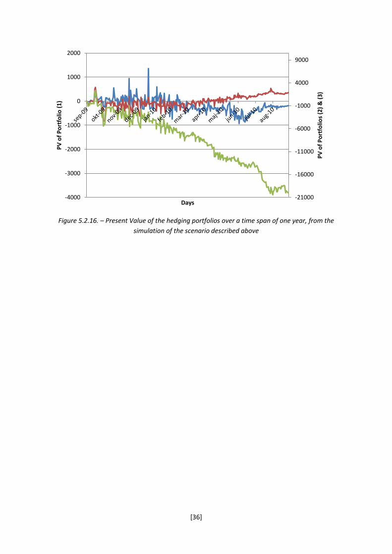
We can see one new result in figure 5.2.16, which is the fact that both portfolio (1) and (2) have
generated a larger loss than what was generated by only the OIS rates in section 5.2.3. Recall from
section 5.1.4., that we saw the cross dependence from OIS rates and LIBOR rates. This is also why we
end up with a loss, even though we are back to being well hedged in terms of the swaps.
-200000
0
200000
400000
600000
800000
1000000
PV
of
Co
ntr
acs
(1),
(2
) &
(3
)
Days
[36]
Figure 5.2.16. – Present Value of the hedging portfolios over a time span of one year, from the
simulation of the scenario described above
-21000
-16000
-11000
-6000
-1000
4000
9000
-4000
-3000
-2000
-1000
0
1000
2000
PV
of
Po
rtfo
lios
(2)
& (
3)
PV
of
Po
rtfo
lio (
1)
Days

[37]
5.2.5. Analyzing the hedge
We have previously established that the efficiency of our hedged portfolio changes as time passes. At
time we are well hedged, but, as we have seen in the previously presented results, we seem to be
partly unhedged for a period of time, until we reach one year, where we once again are well hedged.
This means that swaps, like many other derivatives such as various types of options, should be
dynamically hedged, rather than statically hedged. This also means that we should measure the risk
every day, and add more instruments, so that we stay perfectly hedged.
When running the simulations we have also analyzed how the portfolio should be hedged over time,
i.e. for every iteration we have used the method described in section 3.3. to identify the risk, and
calculate the needed hedging portfolio. So instead of dynamically re-hedging the portfolio every day,
we have kept the initial hedged portfolio, and measured how the effectiveness has changed over
time, by identifying what needs to be added for the hedge to become perfect again.
Whenever we, according to the model, are perfectly hedged (note that this still does not take the
cross dependence and the convexity of the OIS rates into account), all the risks are equal to zero, and
no additional hedge is needed. This will be the case at time , since we, by definition constructed
our portfolio so that we would be perfectly hedged.
Recall that we were supposed to hedge the 0D90M
swap with the weights shown in the chart to the
right (the notional was €10.000.000 and the scale
on the Y-axis is in millions of euros). Figure 5.2.17.
shows how the effectiveness of the hedge gets
worse over time. The Y-axis represents how much
of each instrument that is needed to be added to
the portfolio for it to be perfectly hedged relative
to how much of this instrument we already have
(e.g. if we have €1000 7Y swaps in our portfolio, and €500 has to be added, the graph will show 0,5).
Figure 5.2.17. – The effectiveness of the hedge
-2
-1,5
-1
-0,5
0
0,5
1
1,5
2
2,5
3
3,5
20
09
-09
-29
20
09
-10
-29
20
09
-11
-29
20
09
-12
-29
20
10
-01
-29
20
10
-02
-28
20
10
-03
-31
20
10
-04
-30
20
10
-05
-31
20
10
-06
-30
20
10
-07
-31
20
10
-08
-31
Effe
ctiv
en
ess
of
he
dgi
ng
con
trac
ts
Days
6Y
7Y
8Y
9Y
-6
-4
-2
0
2
4
6
5Y 6Y 7Y 8Y 9Y 10Y
[38]
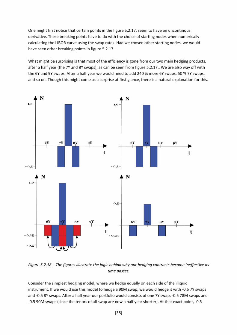
One might first notice that certain points in the figure 5.2.17. seem to have an uncontinous
derivative. These breaking points have to do with the choice of starting nodes when numerically
calculating the LIBOR curve using the swap rates. Had we chosen other starting nodes, we would
have seen other breaking points in figure 5.2.17..
What might be surprising is that most of the efficiency is gone from our two main hedging products,
after a half year (the 7Y and 8Y swaps), as can be seen from figure 5.2.17.. We are also way off with
the 6Y and 9Y swaps. After a half year we would need to add 240 % more 6Y swaps, 50 % 7Y swaps,
and so on. Though this might come as a surprise at first glance, there is a natural explanation for this.
Figure 5.2.18 – The figures illustrate the logic behind why our hedging contracts become ineffective as
time passes.
Consider the simplest hedging model, where we hedge equally on each side of the illiquid
instrument. If we would use this model to hedge a 90M swap, we would hedge it with -0.5 7Y swaps
and -0.5 8Y swaps. After a half year our portfolio would consists of one 7Y swap, -0.5 78M swaps and
-0.5 90M swaps (since the tenors of all swap are now a half year shorter). At that exact point, -0,5
[39]
90M swaps could instead be represented by -0.25 7Y swaps and -0.25 8Y swaps. In the same way the
78M swap could be represented by 6Y and 7Y swaps. Finally, the resulting portfolio is actually -0.25
6Y swaps, 0,5 7Y swaps and -0.25 8Y swaps, which leaves us quite unhedged against a change in any
one of the mentioned contracts, but still well hedge against a parallel shift (if all interest rates move
together). This is why we saw large fluctuations after a half year in the hedging portfolios in sections
5.2.2. and 5.2.5, but is panned out after one year.
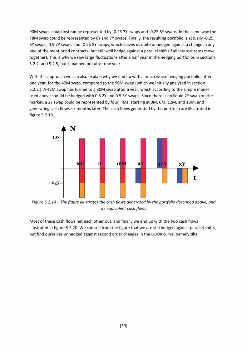
With this approach we can also explain why we end up with a much worse hedging portfolio, after
one year, for the 42M swap, compared to the 90M swap (which we initially analyzed in section
5.2.2.). A 42M swap has turned to a 30M swap after a year, which according to the simple model
used above should be hedged with 0.5 2Y and 0.5 3Y swaps. Since there is no liquid 2Y swap on the
market, a 2Y swap could be represented by four FRAs, starting at 0M, 6M, 12M, and 18M, and
generating cash flows six months later. The cash flows generated by the portfolio are illustrated in
figure 5.2.19..
Figure 5.2.19 – The figure illustrates the cash flows generated by the portfolio described above, and
its equivalent cash flows
Most of these cash flows net each other out, and finally we end up with the two cash flows
illustrated in figure 5.2.20. We can see from the figure that we are still hedged against parallel shifts,
but find ourselves unhedged against second order changes in the LIBOR curve, namely tilts.
[40]
Figure 5.2.20. – The figure illustrates the remaining un-netted cash flows
At time we are supposed to be perfectly hedged. The reason for this is that a price for a, for
example, 90M swap does not exist on the market, and therefore can only be priced in the model.
Therefore, per definition, we are perfectly hedged, for swaps, at the initiation of the contract (which
is not true for the OIS rates though, because of their convexity, which we could see from the intraday
simulations). But when time passes, and the tenors of our contracts change, we are no longer
perfectly hedged, which we have illustrated in the figure 5.2.19.
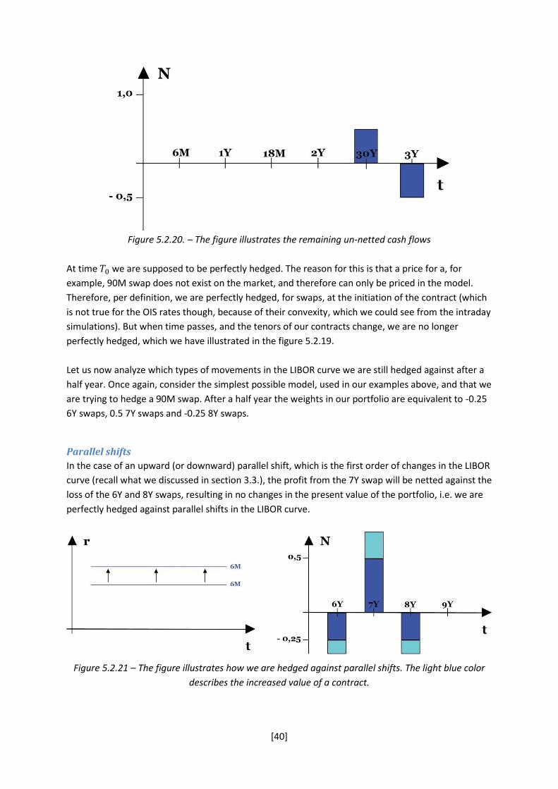
Let us now analyze which types of movements in the LIBOR curve we are still hedged against after a
half year. Once again, consider the simplest possible model, used in our examples above, and that we
are trying to hedge a 90M swap. After a half year the weights in our portfolio are equivalent to -0.25
6Y swaps, 0.5 7Y swaps and -0.25 8Y swaps.
Parallel shifts
In the case of an upward (or downward) parallel shift, which is the first order of changes in the LIBOR
curve (recall what we discussed in section 3.3.), the profit from the 7Y swap will be netted against the
loss of the 6Y and 8Y swaps, resulting in no changes in the present value of the portfolio, i.e. we are
perfectly hedged against parallel shifts in the LIBOR curve.
Figure 5.2.21 – The figure illustrates how we are hedged against parallel shifts. The light blue color
describes the increased value of a contract.

[41]
Tilts
In the case of a tilt, which represent the second order of changes in the LIBOR curve, we see that the slope of the curve changes. Here we see that the profits from the longer swaps net the losses from the shorter swaps, leading to no change in the hedging portfolio, i.e. we are also hedged against tilt changes in the LIBOR curve.
Figure 5.2.22 – The figure illustrates how we are hedged against tilts. The red color describes the
decreased value of a contract.
Humps/Twists
The event of a change in the curvature, which is represented by the third order of changes in the
LIBOR curve, is usually referred to as a hump or a twist. In figure 5.2.23. we can see that we are no
longer hedged against these types of changes in the swap rates, since the value changes of the
instruments are no longer netted against each other.
Figure 5.2.23. – The figure illustrates how we are hedged against twists/humps
We are also not hedged against single interest rate changes, i.e. if one interest rate changes, while
the others stay constant, which is a very unusual type of interest rate change.
Table 5.2.1. – The table describes how we are perfectly hedged in the first and second order of
changes, but not against the third order of changes.
[42]
Many studies have been made on principal component analysis, which tries to analyze which types of
interest rate movements are the most common, and most of them agree on that about 80% to 90 %
of the variance is explained by parallel shifts, while approximately 90% to 95 % of the variance is
explained by all first three orders of changes in the LIBOR curve. The rest of the variance is often
considered as random noise and will usually be excluded from further analysis [James & Webber].

[43]
5.3. Dynamic Hedging Swaps, FRAs, Deposit: Market Data OIS: Constant at 0 % As we can from the results in sections 5.2.2. and 5.2.4. see that the volatility of the hedging portfolio seems to be much larger after a half year, than in the beginning and end of the year. This makes it really tempting to use a strategy where you dynamically re-hedge your portfolio to keep the volatility low. For this reason we have analyzed the present value, over a timespan of a year, which uses the following strategy:
- At time we buy a 90M swap, and hedge it the same way as we have done before. - days later, at time , we sell all our hedging instruments, except for our 90M swap (which
is now a D swap), with a potential profit or loss from each sold instrument. - The money received or lost, is invested (or borrowed) with the overnight rate. - At time we once again identify the risks by bumping each rate separately, and buy the
contracts which will perfectly hedge our illiquid instrument. - days later, at time , we do the same thing we did at time .
We have run a simulation of this strategy for different values on , namely 7, 30 and 90, which represent weekly, monthly and quarterly re-hedging, and the generated results are presented in figure 5.3.1.
Figure 5.3.1. – The present value in euros of the dynamically hedging portfolios, with different
rehedging frequencies over a time span of one year, from the simulation of the scenario described above
The reason we have no volatility after a half year is that our 90M swap has turned into a 7Y swap, which is one of the liquid instruments on the market. We can therefore hedge our contract with a 7Y swap, and be perfectly hedged for the rest of the time.
-2500
-2000
-1500
-1000
-500
0
500
1000
1500
2000
2500
PV
of
Po
rtfo
lios
(1),
(2
) &
(3
)
Days
Quaterly
Monthly
Weekly

[44]
We can clearly see that a strategy with dynamic hedging results in a worse outcome than keeping the contracts for one year straight (compare with the charts presented in section 5.2.2.). It does not seem like the frequency of the re-hedging makes any difference on the present value of the portfolio after one year. We have run the same simulation on two other datasets, which has yielded similar results. What the frequency of the re-hedging does seem to impact is the volatility of the portfolio present value. It seems like a more frequent re-hedging strategy results in a lower overall volatility, and indeed, after analyzing the standard deviation of the resulting datasets, we see that a more frequent re-hedge results in a more stable portfolio value over time. Table 5.2.1. shows the average five day standard deviation for the first half year of the time series.
Quaterly Monthly Weekly
Data 1 € 176 € 82 € 61
Data 2 € 171 € 98 € 86
Data 3 € 184 € 75 € 54
Table 5.2.1. – The five day standard deviations of the different re-hedging strategies.
What is most interesting with this result is that we know that we will end up with a portfolio loss if we attempt to re-hedge our portfolio at any time. This basically means that the model fools you, and makes you think that you should re-hedge the portfolio, to get rid of the noise, which is a bad idea. The best strategy is to always keep your swaps in your hedged portfolio for exactly one year, since you know that your swap hedge will be perfect after exactly one year, even though it looks like you are making a huge loss after a half year. In practice, traders would seldom hedge just one contract. Most often they will either keep a position that they think would be profitable over time, or of they want to get rid of all the present risk, hedge a batch of swaps, which is a strategy that is more similar to dynamic hedging, rather than static.

[45]
7. Conclusions The purpose of this thesis was to investigate the properties of interest rate swaps and their optimal hedging portfolios. The results have shown that we are perfectly hedged against the first and second order of changes (parallel shifts and tilts) in the LIBOR curve, but that we become unhedged against the third order of changes (humps/twists) as time goes by. We have also concluded that we are completely unhedged against the cross term, defined in section 5.1.4., and the convex dependence on the OIS rates, of the present value of the hedging portfolio. However these losses are fairly small in relation to the notional of the hedged contract. Furthermore we have seen that though we seem to be badly hedged for the swap part of the portfolio after a half year, we are once again close to perfectly hedged after a year, because of the nature of the contracts we are using in our hedging portfolio. Therefore the model might trick you into re-hedging your portfolio before a full year has passed, which we have shown is not a good idea, since it leads to larger overall losses. In other words, a strategy of dynamic rehedging, though it lowers the volatility of the portfolio, almost always leads to a worse outcome after a full year. This phenomenon introduces another important problem: When you value you position, after a half year, you need to look at the liquidation value (according to rules from the Swedish Financial Supervisory Authority), which can be much lower than the value you for certain know the swap will be worth in the future. I will leave a solution to this problem for further studies. There are many interesting types of contracts, which are outside of the scope of this thesis, which could be of interest for future investigation, such as cross currency swaps, caps, floors and swaptions. A similar model and methodology could be used to analyze these more complex instruments that are more associated with dynamic hedging strategies than plain vanilla interest rates swaps.

[46]
8. Reference List
Books
C. Ekstrand, “Financial Derivatives Modeling”, 2011, Springer J. James, N. Webber, “Interest Rate Modeling”, 2001, Wiley John C. Hall, “Options, Futures and other Derivatives”, 2002, Pearson
Articles
F. Mercurio, “Interest Rates and The Credit Crunch: New Formulas and Market Models”, 2009, Bloomberg QFR
[47]
9. Appendix The price at time of one dollar at time is given by . Therefore the following statement, for yearly compounding interest rates, has to be true:
The derivation is as follows:
( )
By doing a first order Taylor expansion of the right hand term, we get the following equation:
Finally we have derived the LIBOR rate: