the productivity commission aims to
TRANSCRIPT


The Productivity Commission aims to
provide insightful, well-informed and
accessible advice that leads to the best
possible improvement in the wellbeing
of New Zealanders.

Measuring state sector productivity Final report of the measuring and improving
state sector productivity inquiry, volume 2
August 2018

The New Zealand Productivity Commission
Te Kōmihana Whai Hua o Aotearoa1
The Commission – an independent Crown entity – completes in-depth inquiry reports on topics selected by
the Government, carries out productivity-related research and promotes understanding of productivity
issues. The Commission aims to provide insightful, well-informed and accessible advice that leads to the
best possible improvement in the wellbeing of New Zealanders. The New Zealand Productivity Commission
Act 2010 guides and binds the Commission.
Information on the Commission is available at www.productivity.govt.nz
How to cite this document: New Zealand Productivity Commission. (2018). Measuring state sector
productivity. Final report of the measuring and improving state sector productivity inquiry, vol. 2. Wellington:
New Zealand Productivity Commission.
ISBN: 978-1-98-851918-0 (print) ISBN: 978-1-98-851920-3 (online)
This copyright work is licensed under the Creative Commons Attribution 3.0 license. In essence you are free
to copy, distribute and adapt the work, as long as you attribute the source of the work to the New Zealand
Productivity Commission (the Commission) and abide by the other license terms.
To view a copy of this license, visit http://creativecommons.org/licenses/by/3.0/nz/. Please note that this
license does not apply to any logos, emblems, and/or trademarks that may be placed on the Commission’s
website or publications. Those specific items may not be reused without express permission.
Inquiry contacts
Administration Robyn Sadlier
T: (04) 903 5167
Other matters Judy Kavanagh
Inquiry Director T: (04) 903 5165 E: [email protected]
Website
www.productivity.govt.nz
@NZprocom
NZ ProductivityCommission
1 The Commission that pursues abundance for New Zealand.
Disclaimer
The contents of this report must not be construed as legal advice. The Commission does not accept
any responsibility or liability for an action taken as a result of reading, or reliance placed because of
having read any part, or all, of the information in this report. The Commission does not accept any
responsibility or liability for any error, inadequacy, deficiency, flaw in or omission from this report.
Acknowledgements
This guide is a team effort. Commissioners Murray Sherwin, Professor Sally Davenport and Dr Graham
Scott oversaw the inquiry. Judy Kavanagh directed the inquiry team. Dr Patrick Nolan was lead author
of Measuring state sector productivity, with contributions from Huon Fraser, Terry Genet, Nicholas
Green, Mike Hayward, Dave Heatley, Kevin Moar, Sandra Moore and James Soligo. The team are
grateful for the help and support of Louise Winspear and Robyn Sadlier. The Commission would also
like to acknowledge the helpful comment, advice and examples provided by the Ministries of Health,
Justice, Education and Social Development, the New Zealand Police, TAS, The Treasury, State Services
Commission, Statistics New Zealand and Professor Patrick Dunleavy, London School of Economics.

Contents
Glossary ........................................................................................................................................... i
About this guide ............................................................................................................................. 1
1 Key concepts ......................................................................................................................... 1 1.1 Productivity, inputs, outputs and outcomes ............................................................................... 1 1.2 Applying the concept of productivity to public services ........................................................... 2 1.3 Outline: building a productivity measure .................................................................................... 5 1.4 Productivity measurement: the state of the art .......................................................................... 6 1.5 Further information ....................................................................................................................... 8
2 Scoping ................................................................................................................................ 10 2.1 The business case ....................................................................................................................... 10 2.2 The research question ................................................................................................................ 12 2.3 Think about production too ....................................................................................................... 13
3 Collecting data .................................................................................................................... 14 3.1 Use existing data if possible ...................................................................................................... 14 3.2 Privacy and handling issues ........................................................................................................ 16
4 Defining outputs .................................................................................................................. 20 4.1 Outcomes, outputs and activities .............................................................................................. 20 4.2 Measurability of outputs ............................................................................................................. 21 4.3 Coverage of outputs ................................................................................................................... 22
5 Defining inputs .................................................................................................................... 25 5.1 Defining inputs ............................................................................................................................ 25 5.2 Additional considerations .......................................................................................................... 29
6 Cost weighting and price deflation ...................................................................................... 31 6.1 Combining multiple outputs and inputs into single indexes................................................... 31 6.2 Accounting for price changes .................................................................................................... 34
7 Accounting for differences in operating environments and quality changes ....................... 39 7.1 Differences in operating environments ..................................................................................... 39 7.2 Quality adjustment ..................................................................................................................... 42
8 Measuring and checking ...................................................................................................... 47 8.1 Recap: productivity measures .................................................................................................... 47 8.2 Benchmarking ............................................................................................................................. 48 8.3 Bringing it all together ............................................................................................................... 50 8.4 Sense testing results ................................................................................................................... 51
Appendix A Worked example: case study on early childhood education ..................................... 54
Appendix B Worked example: case study on New Zealand Police .............................................. 57
Appendix C Worked example: case study on universities ............................................................ 62
References .................................................................................................................................... 68
Tables and figures
Table 1.1 Challenges in measuring the output of services ............................................................................... 4 Table 1.2 Steps in defining and implementing a productivity measure .......................................................... 5 Figure 1.1 Statistics New Zealand labour and multi-factor productivity indexes, 1996–2015 .......................... 7 Table 3.1 Example service delivery cost components .................................................................................... 16 Table 4.1 Examples of outcomes and outputs ................................................................................................ 21 Table 5.1 Examples of outputs and contributing inputs ................................................................................. 25 Table 5.2 Options for calculating labour input ................................................................................................ 29 Table 6.1 Quality criteria for price deflators .................................................................................................... 35 Table 7.1 Approaches to quality adjusting school data .................................................................................. 43 Table 7.2 Approaches to adjusting health sector data ................................................................................... 44 Table 7.3 Approaches to adjusting data in other sectors ............................................................................... 44 Table 8.1 Productivity questions and measurement techniques .................................................................... 50 Figure A.1 Labour productivity in the teacher-led ECE sectors, adjusted for wage premia for
qualifications, 2001/02 – 2012/13 ..................................................................................................... 56 Table B.1 Total outputs (responses to mental health incidents), 2010/11–2016/17 ...................................... 58 Figure B.1 Productivity of responses to mental health and threatened or attempted suicide incidents,
2010/11–2016/17 ............................................................................................................................... 59 Figure B.2 Police productivity, upper North Island districts, 2010/11–2016/17............................................... 60 Figure B.3 Police productivity, South Island and lower North Island districts, 2010/11–2016/17 .................. 60 Table C.1 Source data, EFTS and PPE for New Zealand universities, 2016 .................................................... 63 Table C.2 First cut: capital stock productivity, 2016 ......................................................................................... 64 Table C.3 University income data, 2016 ............................................................................................................ 64 Table C.4 Second cut: research-adjusted capital stock productivity, 2016 .................................................... 65 Table C.5 University depreciation, 2016 ........................................................................................................... 65 Table C.6 Third cut: research-adjusted capital flow productivity, 2016 .......................................................... 66 Table C.7 Fourth cut: casemix- and research-adjusted capital flow productivity, 2016 ................................ 67
Glossary i
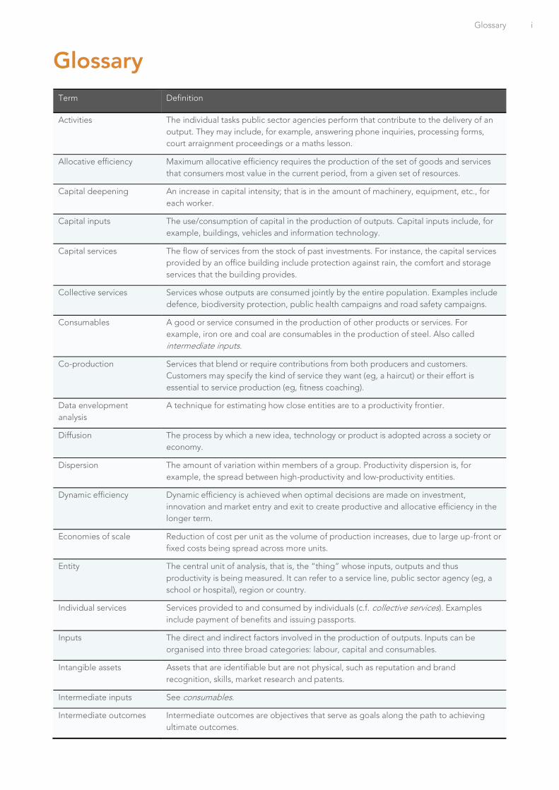
Glossary
Term Definition
Activities The individual tasks public sector agencies perform that contribute to the delivery of an
output. They may include, for example, answering phone inquiries, processing forms,
court arraignment proceedings or a maths lesson.
Allocative efficiency Maximum allocative efficiency requires the production of the set of goods and services
that consumers most value in the current period, from a given set of resources.
Capital deepening An increase in capital intensity; that is in the amount of machinery, equipment, etc., for
each worker.
Capital inputs The use/consumption of capital in the production of outputs. Capital inputs include, for
example, buildings, vehicles and information technology.
Capital services The flow of services from the stock of past investments. For instance, the capital services
provided by an office building include protection against rain, the comfort and storage
services that the building provides.
Collective services Services whose outputs are consumed jointly by the entire population. Examples include
defence, biodiversity protection, public health campaigns and road safety campaigns.
Consumables A good or service consumed in the production of other products or services. For
example, iron ore and coal are consumables in the production of steel. Also called
intermediate inputs.
Co-production Services that blend or require contributions from both producers and customers.
Customers may specify the kind of service they want (eg, a haircut) or their effort is
essential to service production (eg, fitness coaching).
Data envelopment
analysis
A technique for estimating how close entities are to a productivity frontier.
Diffusion The process by which a new idea, technology or product is adopted across a society or
economy.
Dispersion The amount of variation within members of a group. Productivity dispersion is, for
example, the spread between high-productivity and low-productivity entities.
Dynamic efficiency Dynamic efficiency is achieved when optimal decisions are made on investment,
innovation and market entry and exit to create productive and allocative efficiency in the
longer term.
Economies of scale Reduction of cost per unit as the volume of production increases, due to large up-front or
fixed costs being spread across more units.
Entity The central unit of analysis, that is, the “thing” whose inputs, outputs and thus
productivity is being measured. It can refer to a service line, public sector agency (eg, a
school or hospital), region or country.
Individual services Services provided to and consumed by individuals (c.f. collective services). Examples
include payment of benefits and issuing passports.
Inputs The direct and indirect factors involved in the production of outputs. Inputs can be
organised into three broad categories: labour, capital and consumables.
Intangible assets Assets that are identifiable but are not physical, such as reputation and brand
recognition, skills, market research and patents.
Intermediate inputs See consumables.
Intermediate outcomes Intermediate outcomes are objectives that serve as goals along the path to achieving
ultimate outcomes.
ii Improving state sector productivity
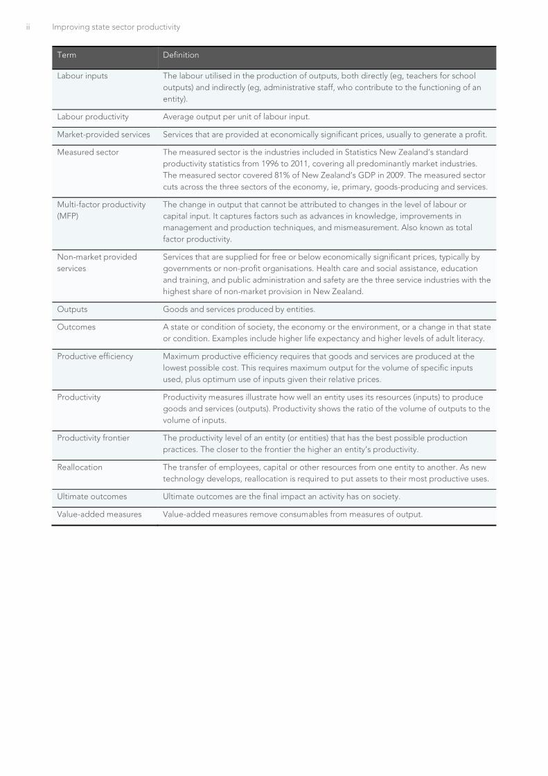
Term Definition
Labour inputs The labour utilised in the production of outputs, both directly (eg, teachers for school
outputs) and indirectly (eg, administrative staff, who contribute to the functioning of an
entity).
Labour productivity Average output per unit of labour input.
Market-provided services Services that are provided at economically significant prices, usually to generate a profit.
Measured sector The measured sector is the industries included in Statistics New Zealand’s standard
productivity statistics from 1996 to 2011, covering all predominantly market industries.
The measured sector covered 81% of New Zealand’s GDP in 2009. The measured sector
cuts across the three sectors of the economy, ie, primary, goods-producing and services.
Multi-factor productivity
(MFP)
The change in output that cannot be attributed to changes in the level of labour or
capital input. It captures factors such as advances in knowledge, improvements in
management and production techniques, and mismeasurement. Also known as total
factor productivity.
Non-market provided
services
Services that are supplied for free or below economically significant prices, typically by
governments or non-profit organisations. Health care and social assistance, education
and training, and public administration and safety are the three service industries with the
highest share of non-market provision in New Zealand.
Outputs Goods and services produced by entities.
Outcomes A state or condition of society, the economy or the environment, or a change in that state
or condition. Examples include higher life expectancy and higher levels of adult literacy.
Productive efficiency Maximum productive efficiency requires that goods and services are produced at the
lowest possible cost. This requires maximum output for the volume of specific inputs
used, plus optimum use of inputs given their relative prices.
Productivity Productivity measures illustrate how well an entity uses its resources (inputs) to produce
goods and services (outputs). Productivity shows the ratio of the volume of outputs to the
volume of inputs.
Productivity frontier The productivity level of an entity (or entities) that has the best possible production
practices. The closer to the frontier the higher an entity’s productivity.
Reallocation The transfer of employees, capital or other resources from one entity to another. As new
technology develops, reallocation is required to put assets to their most productive uses.
Ultimate outcomes Ultimate outcomes are the final impact an activity has on society.
Value-added measures Value-added measures remove consumables from measures of output.

About this guide iii
About this guide
Productivity is a measure of the goods and services produced (outputs) by an economy, industry or
organisation compared to the resources used in that production (inputs). Improving productivity is about
making better use of inputs; producing more or better outputs with the same resources. It is not about
increasing hours of work or cutting budgets. Neither of these will produce a measurable increase in
productivity. Valid productivity measures account for changes in the quality of outputs. For example, a
budget reduction (lower inputs) that leads to a reduction in quality (reduced output) is unlikely to boost
measured productivity.
Measures of productivity have their origins in the private sector. The methods and concepts developed for
measuring private sector productivity typically rely on assumptions that may not be valid in the state sector.
This does not make state sector productivity measurement impossible. It simply means that you may need to
apply different measurement techniques than those you would use to study the private sector.
Productivity measurement can be applied to a whole agency, to a functional unit, or to specific activities and
programmes. An organisation that measures productivity is in a better position to know if it is achieving the
best outcomes it can with the resources it uses. Without such measures it is difficult to know whether the
organisation’s performance is improving or declining.
The Commission has developed this guide to help people in the state sector to measure the productivity of
their agencies, functional units, activities and programmes. This guide is part of the final report of the
Commission’s inquiry into measuring and improving state sector productivity. You can read it independently
or in conjunction with Improving state sector productivity.
The Commission wrote this guide primarily for individuals and teams within the state sector who are
intending to develop productivity metrics. You should also find this guide useful if commissioning or
evaluating productivity studies, or just understanding the productivity measures created by others.
The guide does not present a one-size-fits-all approach. It aims to give practical advice on how to better
understand your organisation and its performance. It assumes you already have a basic knowledge of
productivity measurement concepts. The glossary may be useful to refresh or clarify these concepts and the
terms used in the guide. This guide has eight chapters.
Chapter 1 outlines important concepts, such as what is productivity, how it relates to outcomes, and how
it can apply to state sector services.
Chapters 2 and 3 discuss practical considerations in the development of productivity measures, including
the need to establish what the measures will be used for, developing a clear research question, and
planning the use of data.
Chapters 4 and 5 discuss outputs and inputs, respectively. These chapters cover their definition and
measurement.
Chapter 6 then explains how to combine different outputs and inputs into a single index. This is
necessary when measures cover more than just single outputs or inputs. The chapter also outlines the
ways to account for price changes.
Chapter 7 outlines approaches to accounting for differences in operating environments and when the
quality of outputs and inputs change over time.
Chapter 8 pulls the guide together by discussing the types of measures to use and benchmarking
techniques. It also covers triangulating (sense testing) results with the findings of quantitative and
comparative studies.
Measuring state sector productivity is a developing field. This a living document, which the Commission
intends to update as the techniques for measuring state sector productivity evolve. The Commission invites
your feedback to improve future editions. Please send suggestions to [email protected]


Chapter 1 | Key concepts 1
1 Key concepts
This chapter outlines the concepts behind productivity measurement, how they relate to outcomes, and how
they apply to public services. The chapter also discusses state-of-the-art state sector productivity
measurement, and its evolution from the “outputs equals inputs” convention. It discusses the role of
aggregate data and micro-level data. It outlines productivity path analysis as one approach to measurement.
1.1 Productivity, inputs, outputs and outcomes
Public services make up close to one fifth of the economy and so poor productivity in this sector is a drag on
the New Zealand economy (both in its own right and in terms of impact on the performance of the private
sector). More productive public services offer governments improved choices and higher living standards for
New Zealanders.
Productivity is a measure of how efficiently an economy, industry or organisation produces goods and
services (outputs) using inputs such as labour and capital. More specifically, it shows the relationship
between the volume of output produced and the volume of inputs consumed in that production.
Volume, in this context, is a measure of quantity. You can measure volume directly, for example, the number
of hours worked, or number of widgets produced. More typically, you will need to convert volume measures
to dollar amounts and adjust them for factors like quality. Subsequent chapters outline procedures for doing
this.
Productivity measures can show how well an organisation uses its resources, both over time and compared
to similar organisations. Such comparisons can provide you with useful insights about where and how to
improve organisational performance.
Box 1.1 Should you use partial or multi-factor productivity measures?
Measuring the productivity of a single input (eg, labour) can provide valuable insights into
performance. Such measures are called partial productivity measures. However, partial productivity
measures can be misleading if the contribution of other inputs changes over time.
For example, suppose a measure of labour productivity shows a consistent increase in output per
worker over time. The increase could be due to management practices, such as hiring more highly
skilled staff or introducing new processes. But it could also be due to investment in technology (ie, a
capital investment). Basing productivity measures on only labour inputs could mis-attribute the
underlying cause of the measured productivity improvement. Worse, if the new technology was costly
relative to the labour saved, overall productivity – in terms of all resources consumed – may have
declined.
Technology is already shaping the delivery of many public services. Taxpayers submit their tax returns
online. Airports have automated passport checks (SmartGate). Doctors increasingly provide services
through patient portals and virtual consultations. It is likely that much of the future growth in state
sector productivity will involve further investments in technology. Given this, productivity measures can
be useful if they incorporate other contributing factors, especially capital and, in some cases,
consumables. Such measures are termed multi-factor productivity measures.
Data limitations may mean that it is difficult (or impossible) to measure capital inputs (see Chapter 5)
and so it may be more practical to measure labour productivity. Given the labour intensity of many
public services, labour productivity may be a good proxy for the overall performance of these services.
However, you should be aware of the limitations of such partial productivity measures.
2 Improving state sector productivity
There is widespread misunderstanding of the concept of productivity. It is about making the best possible
use of resources like labour and funding, not increasing hours of work or cutting budgets. Properly
measured, it should account for factors like changes in the quality of inputs and outputs.
Productivity is one dimension of performance
Performance frameworks for state sector agencies should include productivity as one dimension. It is not
possible to achieve the best possible outcomes for New Zealanders unless public services are productive
(Smith, 2018). It may, for instance, be possible to decide what outcomes are desired and to even predict the
likely contribution of specific outputs to these outcomes. But unless the state sector can effectively convert
the resources available into outputs it will fail to maximise desired outcomes with the resources available.
To put this more technically, the state sector cannot be allocatively efficient (on the optimal point on its
current production possibility frontier) or dynamically efficient (expanding the frontier over time) unless it is
also productive. But this also goes in the other direction. As Richardson (2012, p. 276) noted:
the real reform of the public sector is only going to come when governments knuckle down to the real
task of defining first what the state should (and should not) do, before embarking on the crusade for a
smarter state. No point in the state doing dumb things in a smarter way.
Thus, a desire to both maximise productivity and to ensure allocative and dynamic efficiency are central to
optimising the performance of the state sector. They are complements, not substitutes.
1.2 Applying the concept of productivity to public services
It is inappropriate to take the methods and concepts developed for measuring private sector productivity
and to uniformly apply them to public services (Box 1.2). This does not mean that state sector productivity
cannot be measured. It simply means that productivity in the state sector needs to be measured differently
to how it is measured in the private sector. This section discusses some of these differences: the nature of
the labour input, accountability for inputs, the observability of outputs and the role of reallocation.
The nature of the labour input
Public services tend to be relatively labour intensive. This means they can face the “Baumol cost disease”,
where wage growth in labour-intensive industries becomes decoupled from productivity growth (Baumol &
Bowen, 1966). This can happen when productivity improvements in a capital-intensive industry lead to wage
growth in that industry. Competition for labour between this industry and other more labour-intensive
industries can lead to wages in these other industries growing too. This increases the cost of labour inputs
relative to the outputs produced and leads to lower labour productivity. Some service industries are
particularly prone to this “disease”.
Workers in the private and state sectors often receive different forms of financial rewards. State sector
workers are more likely to have standardised pay scales – with constraints on pay levels and fewer incentives
tied to performance – and greater job security. They typically have no claim on profits or cost savings. Some
argue that state sector workers face greater non-pecuniary incentives, such as concern about their
reputation, mission orientation, etc. According to this view, state sector workers are relatively more
motivated by non-financial rewards, such as a shared sense of mission.
Box 1.2 Measuring productivity of the private sector
The concepts and methods of productivity measurement were originally developed to apply to the
private sector. Much of the terminology reflects a “factory” model of production. Despite the
terminology, the concepts generalise well to other production models and to services. Nonetheless,
analysts of private sector activities and organisations typically make assumptions that simplify data
collection and analysis. These can include assuming market prices approximate the opportunity cost of
inputs and outputs. In turn, this assumes no subsidies, and no monopoly production nor monopsony
purchasing.

Chapter 1 | Key concepts 3
In practice differences in motivation of private and state sector workers are less clear cut (Le Grand, 2007).
Non-financial rewards motivate many people working in the private sector, and it is naive to say state sector
workers do not have financial motivations. The private sector produces many essential goods and services
(eg, food). Others are produced by both the private and state sector (eg, education and health).
Relying on the mission orientation of state-sector workers may not always lead to productive services.
“Knightly” people may not “always be motivated to be very efficient” (eg, recognise the opportunity cost of
the resources they consume) and may have their own agenda (eg, “give users what the knights think users
need, but not necessarily what the users think they need”) (Le Grand, 2007, pp.20-21).
The uniqueness of the labour input into public services can be overstated. Many of the techniques used to
account for labour input in the private sector are applicable to public services. However, be careful when
using wage rates to cost weight different categories of workers (a technique used in the private sector) as
these rates can be set in differently in the two sectors (see Chapter 5).
Accountability constraints
A further difference between the private and state sectors reflects the importance of accountability for
inputs. A principle of the state sector reforms in New Zealand in the 1980s was to increase the flexibility with
which state-sector managers could manage inputs. The principle was that the political executive would
specify desired outcomes, contract agency chief executives for outputs to contribute to these outcomes, and
agencies would then manage the inputs to achieve them (letting “managers manage”). Nonetheless, the
allocation of inputs (eg, workers) in the state sector is subject to public law and administrative requirements.
These are designed to ensure that public funds are used in a lawful, transparent and accountable manner.
Agencies may manage performance risk through highly specified contracts that describe the inputs used,
the processes followed, and the outputs produced (NZPC, 2015). This reduces incentives and opportunities
for innovation, limits the flexibility of providers to respond to changing needs of service recipients or
changes in the wider environment, and limits the scope for providers to work together and to bundle
services in a way that best meets the needs of recipients (ie, service integration).
This has implications for measuring productivity in the state sector. You should seek to understand the
extent that productivity estimates reflect controls over the ways that inputs are managed. An observed
change in productivity may reflect a change in public policy rather than choices made by managers per se.
This is one reason why state-sector productivity measures should be treated as one input into performance
decisions, rather than the sole factor (Tavich, 2017).
Management literature distinguishes between high- and low-powered incentives. High-powered incentives
tie significant private rewards (or sanctions) to measured outputs or outcomes. For example, salespeople
often receive a low base salary plus a commission on each sale they close. High-powered incentives can be
effective to motivate staff where a goal is clearly measurable and well aligned with an organisation’s overall
purpose, the factors that influence the measure are under control of the staff concerned, and zealous pursuit
of the reward is unlikely to create perverse consequences. Low-powered incentives are appropriate if
multiple goals are sought, results are difficult to measure, teamwork is crucial, or success is determined by
factors beyond the staff’s control. Public services rarely meet the criteria for high-powered incentives.
Reflecting this, the state sector generally offers its employees salary packages with low-powered incentives.
However, high-powered incentives can feature in public service provision if status, continuation of
employment, promotion prospects or other non-salary remuneration are conditional on performance
measures. It is important to recognise such situations and manage potentially adverse consequences.
Observability of outputs
It is generally harder to measure outputs in the services sector, as compared to the manufacturing and
primary sectors. This applies to production by the state and private sectors. Table 1.1 sets out some of the
challenges in measuring the productivity of services.

4 Improving state sector productivity
Table 1.1 Challenges in measuring the output of services
Issue Implications
Service output is “fuzzy”. The process
of producing a service does not result
in a tangible good but in a “change of
state”
It can be hard to clearly identify the output of a service
It might be difficult to separate the output of services from factors used
in its production (ie, distinguishing the output from the process)
It can be challenging to identify quality improvements
Some service outputs are co-produced
with customers. Customers often
determine what kind of service they
want (eg, a haircut) or their effort is
essential in producing the service (eg, a
fitness programme)
Problems defining and identifying a standardised unit of output, as the
customer’s involvement in production means each output is different
and adapted to specific needs
Difficulties identifying the value added by the provider, as opposed to
the customer
For some services, particularly social
services, the purchaser and the
customer are different people or
entities
The purchaser’s assessment of quality and value may be different from
the customer’s assessment
Source: Djellal and Gallouj, 2008; NZPC, 2015.
Estimates of private-sector productivity generally use price information to:
judge the relative value of different goods and services;
account for changes in the quality of outputs; and
weight different goods and services when aggregating data (eg, into industry or national measures).
However, for many public services there is no price information (as services are free to the consumer) or only
limited price data (as they are subsidised or not in a competitive market) (Dunleavy, 2016). You will need to
apply different techniques when comparing or aggregating state sector activities, and when accounting for
changes in quality (see Chapters 6 and 7).
Private-sector firms typically have straightforward goals like increased market share or shareholder value.1 By
contrast, some state-sector services have relatively complex goals. These encompass, for example, concerns
about who benefits (Tavich, 2017).
Even where agencies have clear high-level goals (eg, to increase human capital), it is difficult to define
measurable indicators of performance for co-produced services. Public services are also likely to have
multiple consumers – those directly receiving the service (eg, patients, schoolchildren) and the wider
citizenry – who may have different perspectives on a specific service.
It is also important to consider what is driving observed changes in productivity and, if necessary, how these
results compare with other sources of evidence. This is why Atkinson (2005) emphasised the need to
supplement productivity measures with independent evidence – what he called a process of “triangulation”.
Resource allocation works differently
A significant portion of productivity growth in the private sector is the result of influences that are external to
individual firms (Conway, 2016). For example, competition between suppliers encourages firms to drive
down production costs and/or improve product quality. Preferences by consumers for cheaper or better
products can shift market share towards more productive firms at the expense of the less productive ones.
Inputs (consumables, labour and investment capital) follow the market share, shifting to the firms with higher
1 This is not to say that such goals are easily achieved, nor that they can be achieved without staying on the right side of suppliers, customers, employees,
governments, etc. However, for analytical purposes it is usually reasonable to model private firms as if they had a single-valued objective.

Chapter 1 | Key concepts 5
productivity where they are, in turn, used more efficiently than previously. Such “reallocation” improves in
the measured productivity of that industry.
Some of these external influences do not apply as strongly (if at all) to the state sector (Dunleavy, 2015). For
instance, competition (either in output markets or for the ownership of the firm itself) is often absent in the
state sector. Many of the agencies that deliver public services face little competition. And while governments
can restructure, merge, split or disestablish state-sector agencies, this tends to be slower and harder to do
than in the private sector. Structural change in the state sector is typically motivated by multiple goals, some
of which are incompatible with improved productivity. The need to satisfy multiple stakeholders places
further constraints on structural changes.
In response to societal demands for better outcomes (eg, in mental health), politicians and state-sector
agency leaders may direct increased resources towards ineffective or inefficient services. Should those
resources come from the budgets of relatively more productive services, then reallocation effects lead to an
overall drop in state-sector productivity. This is the opposite result from the reallocation effects in the private
sector, as described above.
Reflecting these considerations, state sector productivity growth is much more likely to rely on technological
diffusion, defined broadly (Dunleavy, 2013). Fortunately measuring diffusion in the state sector is often a
relatively straightforward exercise. Many administrative systems hold the data required to directly measure
changes in practices. This contrasts with private firms where innovation cannot often be directly observed –
measures of the number of firms engaged in innovative activity can range from 0.2% to 40% (Wakeman & Le,
2015).
1.3 Outline: building a productivity measure
Table 1.2 outlines the steps you will need to undertake – or at least consider – in defining and implementing
a productivity measure, along with the relevant chapter for each step. For simpler measures you may be able
to omit some steps.
While this guide describes this approach as a linear process, in practice it is likely to be iterative. You should
refine the analysis as understanding and availability of data change over time.
Table 1.2 Steps in defining and implementing a productivity measure
Step Considerations Chapter
Scope
Establish the
business case
Establish the benefits of measuring productivity; the ongoing resource commitment;
how measures will be used and released; the role of staff in development and
refinement; and risks that measures could be misunderstood or create harmful
incentives
2
Develop a clear
research question
Define the entity being studied; whether different entities will be compared; whether to
measure productivity levels and/or growth rates; whether measures will be undertaken
for a single period or repeated; whether partial and/or multi-factor productivity
measures are most useful; and whether value-add or gross productivity measures are of
interest
2
Prepare
Establish what
data you need
Establish rules, protocols and procedures regarding the use of data; what existing data
are available and how existing data map to the research question; whether data gaps
can be addressed by linking existing datasets; and, if new data are needed, does their
collection pass a cost-benefit test
3

6 Improving state sector productivity
Step Considerations Chapter
Define and
measure outputs
Establish the appropriate level for defining inputs (eg, service line, individual provider,
across several providers); which outputs can be measured; how
representative/important the measured outputs are; whether the exclusion of some
outputs biases the measure; and how to account for unmeasured outputs
4
Define and
measure inputs
Establish how detailed data on inputs need to be; which inputs can be measured and
whether exclusions bias the measure; how inputs can be apportioned to outputs
5
Convert diverse
outputs and
inputs into a
consistent format
If valid market prices exist then use these to combine (weight) multiple outputs (or
inputs) into a single index, otherwise use per-unit production costs (cost weights).
Generally, use publicly available price indexes (such as the full CPI) to deflate
expenditure figures. The approach taken must be transparent as it can have a major
impact on results
6
Standardise inputs
and outputs
Establish whether the quality of services or the operating environment are likely to have
changed and whether these changes will affect the measure. You can account for
changes by segmenting services or users into groups with similar characteristics. Other
approaches include assessing the impact on intermediate outcomes (for quality) or
changes in population characteristics (for the operating environment). The approach
taken must be transparent as it can have a major impact on results
7
Produce
Measure Following the scoping and preparation stages, undertake the productivity
measurement. Compare productivity performance, across time and across entities. It is
useful to start with simple measures and develop more complex approaches over time
8
Check Discuss findings widely at draft stage and benchmark findings against similar studies.
Follow a clear process for releasing and updating results
8
1.4 Productivity measurement: the state of the art
For many years, the default position in measuring the output of the state sector was to assume the growth
rate of outputs was equal to the growth of inputs (implying no change in productivity). This is the “inputs
equals outputs” convention. This convention reflected the absence of price data and easily observable
output measures for publicly produced goods and services. This convention effectively assumes away the
question of productivity. It implies that the social value of government outputs always grows at the same rate
as the cost of inputs.
Since the early 2000s, many governments have made efforts to move beyond the inputs equals outputs
convention. An improved understanding of productivity measurement and advances in data collection and
analytics has supported these efforts (Dunleavy, 2016). The Office for National Statistics (ONS) in the United
Kingdom has been at the forefront. Impetus came from an independent review of the measurement of
government output and productivity commissioned in 2003 by the ONS and led by Sir Anthony Atkinson.
This followed a European Commission requirement that national accounts should incorporate direct
measures of government output. Valuable progress has also been made in New Zealand (see Box 1.3).
This guide outlines an approach to productivity measurement based on Productivity Path Analysis (PPA)
(Dunleavy, 2016). This approach differs from the aggregate approach taken by Statistics New Zealand (Box
1.3). The advantage of aggregate measures is that they are potentially comprehensive. A limitation is that
they do not address the distribution of outcomes across entities within a sector. In contrast, micro-data
approaches like PPA can provide a relatively rich picture of service productivity and help illustrate important
policy questions (such as the variation of performance across organisations). But these approaches can be
data and resource intensive, and each study only provides a partial view of changes in aggregate state sector
productivity.

Chapter 1 | Key concepts 7
The approach in this guide is consistent with the principles for measuring state sector productivity set out in
the Atkinson report (2005). Although that report focused on measuring state sector productivity in the
system of national accounts, its recommendations reflected best practice more generally. Atkinson argued
that approaches to measuring state sector productivity should contain the following features.
Box 1.3 Statistics New Zealand measures of state sector productivity
Statistics New Zealand regularly publishes estimates for education and training, and health care and
social assistance, as part of their annual releases of industry-level productivity measures. Statistics
New Zealand (2013) and Tipper (2013) detail the methodology.
Tipper (2013) noted education and health care became priorities for Statistics New Zealand as these are
where most progress has been made in defining output measures. Their output measures are based on
a chain-volume value-added GDP production approach (see section 6.2 for an explanation of chain
weighting). Value add is defined as output minus consumables (see section 5.1 for a discussion on
consumables). Defining output in collective services such as defence, police or fire services remains
relatively difficult and so estimates for these services continue to be based on the “inputs equals
outputs” convention.
Having defined activity measures, their growth rates are calculated. Within subsectors, the growth rates
of unmeasured activities are assumed to be the same as those of measured activities. The growth rates
of the activities are then combined into a single output index for the subsector using cost weights for
the different components of output which reflect their relative importance.
In the case of inputs, measures of labour and capital used in the production of the activities are
estimated and combined. The labour input is based on hours paid, while the capital input is estimated
by applying the user cost of capital to the total capital stock used in the industry. The latter is
constructed using the perpetual inventory method (PIM) (see Box 5.1). An exogenously given rate of
return of 4% is applied to all industries in the estimation of the user cost of capital (Macgibbon, 2010).
Figure 1.1 shows the labour productivity and multi-factor productivity indexes for education and
training, health care and social assistance, and for the measured sector2. While these data are not
explicitly quality adjusted, techniques exist for doing this (see section 7.2). However, in the absence of
international standards for these techniques quality-adjusted measures should not be included in the
national accounts.
Figure 1.1 Statistics New Zealand labour and multi-factor productivity indexes, 1996–2015
Sources: Statistics New Zealand, 2017a; Tipper, 2013.
Notes:
1. Index = 1000 for 1996.
2. The industry coverage of the productivity statistics is defined as the ‘measured sector’. These industries mainly contain enterprises that are market producers. This means they sell their products for economically significant prices that affect the quantity that consumers are willing to purchase (Statistics New Zealand, n.d.).
400
600
800
1000
1200
1400
1996 1998 2000 2002 2004 2006 2008 2010 2012 2014
Labour productivity
Education and Training
Health Care and Social Assistance
Measured sector
400
600
800
1000
1200
1400
1996 1998 2000 2002 2004 2006 2008 2010 2012 2014
Multifactor productivity
Education and Training
Health Care and Social Assistance
Measured sector
400
500
600
700
800
900
1000
1100
1200
1300
1400
1996 1997 1998 1999 2000 2001 2002 2003 2004 2005 2006 2007 2008 2009 2010 2011 2012 2013 2014 2015
Measured sector Education and training Health care and social assistance

8 Improving state sector productivity
Output indicators should cover the full range of services for that functional area.
Outputs should be adjusted for quality, taking account of the attributable incremental contribution of
the service to the outcome.
The measurement of inputs should be as comprehensive as possible and should include capital services.
Independent corroborative evidence should be sought on government productivity, as part of a
“triangulation” process, recognising the limitations in reducing productivity to a single number.
Productivity Path Analysis is consistent with these features.
1.5 Further information
The sources in Box 1.4 are a useful supplement to this guide.
Box 1.4 Looking for more information?
Statistics New Zealand’s (2010) feasibility study Measuring government sector productivity in New
Zealand provides a good introduction to the topic along with an overview of concepts and compilation
challenges. This study also discusses measuring health care and education productivity in some detail.
Likewise, while Statistics New Zealand’s Productivity statistics: sources and methods (10th edition)
(2014) focuses on the approach to measuring productivity in the measured sector, the chapters on the
labour series and capital series can be helpful when measuring state sector productivity.
The Office for National Statistics in the United Kingdom has produced useful guidance material. The
ONS Productivity Handbook (Office of National Statistics, 2007) includes chapters on public service
productivity and quality adjustment. The Atkinson Review: Final Report (Atkinson, 2005) is a valuable
resource and includes chapters on methodological principles, inputs and deflators, outputs and
implementation, along with discussion of measurement issues in state-sector industries (health,
education, public order and safety, and social protection).
Dunleavy and Carrera (2013) provide an overview of Productivity Path Analysis and present UK
examples for several services, including customs, tax, regulatory agencies and hospitals.
A more general summary of the approaches to measuring state sector productivity in different OECD
member countries can be found in Lau, Lonti and Schultz (2017). The OECD has also published useful
technical guidance, including Schreyer’s (2010) Towards measuring the volume of output of education
and health services: A handbook.
The New Zealand Treasury’s Guide to social cost benefit analysis (2015) includes useful material on
topics such as willingness-to-pay approaches and approaches to discounting. Material produced as
part of the development of the Living Standards Dashboard (Janssen, 2018; Smith, 2018) provide a
valuable overview of issues such as how to value financial and physical capital.

Chapter 1 | Key concepts 9
Chapter 1 takeaways
Productivity is a measure of how efficiently an entity converts inputs (typically capital, labour and
consumables) into outputs (such as services). When the state sector produces outputs efficiently,
available resources go further, and the government can achieve improved outcomes. Conversely,
poor state sector productivity can be a drag on the whole economy.
Methods for measuring productivity in the private sector cannot always be used to measure the
productivity of state sector activities. This does not mean state sector productivity is impossible to
measure, only that different approaches are often required.
In the past, governments have assumed state sector outputs increase directly in proportion to
inputs, that is state sector productivity was assumed not to change over time. This “inputs equals
outputs” convention effectively assumes productivity is unchanged and unchangeable.
Governments around the world are moving beyond this convention. The United Kingdom has been
at the forefront of developing methods to measure state sector productivity. New Zealand has also
made useful progress.
Productivity Path Analysis (PPA) is one approach to measuring state sector productivity. This guide
discusses the steps involved in undertaking a PPA:
- clearly establish the productivity question the measure is trying to answer;
- identify the core outputs of the entity being examined, identify the unit cost associated with
each output, then develop a cost-weighted total output metric;
- calculate the total cost of inputs used to produce the outputs; and
- decide whether adjustments need to be made for changes in output quality or changes to the
organisation’s operating environment.

10 Improving state sector productivity
2 Scoping
Designing, measuring, checking, understanding, reporting, responding to and refining a productivity
measure is an iterative process. But it needs to start somewhere. This chapter covers scoping the measure:
establishing a business case and a clear research question.
2.1 The business case
The business case for a productivity measure needs to contain, in broad terms, what will be measured, the
likely start-up and ongoing costs of measurement and what the agency might gain from measurement. The
clearer this is, the easier it will be to get buy-in.
It is valuable to first establish what “business need” the measure will address. Performance measures can
serve a number of distinct purposes (Gill & Schmidt, 2011; van Dooren, Bouckaert & Halligan, 2015). These
include:
to steer and control (eg, whether policies and programmes on track);
to give account (eg, whether performance can be justified); and
to learn (eg, whether improvements can be made).
There can be tension between these roles. Gill and Schmidt (2011) noted that a “focus on accountability and
control tends to punish deviations from standards rather than providing an opportunity to learn” (p.16).
Cooley (1983) argued that “indicators will be corrupted more readily if rewards or punishments are
associated with extreme values on that indicator, than if the indicator is used for guiding corrective
feedback” (p.9).
While accountability and steering are important, the main benefit from productivity measurement is the
potential to encourage conversations and learning about service improvements. These measures should be
used “as a diagnostic [tool] rather than a target” (Gill, Kengema & Laking, 2011, p.433). Where the primary
objective of a measure is to promote learning and improvement it is worth considering:
how directly the results of the measure will lead to a decision or action;
the consequences of any decision that are based on the measure (eg, the significance for funding levels,
managerial flexibility or team reputations); and
whether productivity measures may lead to an incomplete or misleading picture of performance (eg,
because of other, extenuating factors).
Of course, performance information is often used to achieve multiple objectives and the way the information
is used may vary from its intended purpose. The Official Information Act 1982 provides public access to
information, which can enable participation in government and hold governments and state-sector agencies
to account. However, if information is made public without the necessary context, then measures intended
to learn or steer may be used by the public or media for accountability purposes.
This is not a reason to avoid developing productivity measures or to keep them hidden. It simply shows that
state-sector agencies need a clear understanding of what might be inferred from any measures they develop
and to make this explicit when measures are released.
Guiding principles
It is also important that the broader agency environment is conducive to collecting and disseminating
productivity measures. Adopting the following principles can help productivity measurement contribute to
an agency’s objectives:
collect productivity data as part of business-as-usual activity;

Chapter 2 | Scoping 11
productivity measures complement measures of outcomes;
productivity measures are just one input into evaluating performance;
the primary use of productivity measures is to learn about service improvement;
staff who deliver services are involved in designing productivity measures; and
agency leaders actively support the use of productivity measures.
Following these principles will make it easier for agencies to measure productivity and make measurement
more useful (eg, by contributing to existing performance frameworks and outcomes). See the companion
volume to this guide: Improving state sector productivity for a fuller discussion.
Building a receptive culture
State sector leaders need to lay the groundwork for efficiency improvements by demonstrating a
commitment to organisational learning and the use of productivity measures. There are several ways that the
use of productivity measures can be encouraged. Box 2.1 lists some suggestions. Further detail on policy
and leadership needed to establish receptive culture for measuring productivity is in the companion volume
Improving state sector productivity.
Involve the staff who deliver services in the development of measures
Measures developed with staff are more likely to reflect the reality of service delivery and be more accurate,
trusted, sustainable, and more effectively implemented and used. Knopf (2017) noted in her review of
efficiency measurement in the health sector that the “workforce has strong views and most of the expertise
on the best way to provide services. They are critical to implementing service improvements” (p. 14).
Involving staff in the development and implementation of measures can help manage any undesirable
effects they may create. Employee engagement in the development of organisational measures and
strategies is also important for promoting higher performance, innovation and staff wellbeing (OECD, 2016).
Box 2.1 How leaders can create a receptive culture for productivity measures
Regularly and consistently pay attention to and prioritise organisational learning and the pursuit of
efficiency and effectiveness.
Provide a role model for officials and coach other leaders in how to encourage learning and
efficiency throughout the organisation.
Put in place organisational systems and procedures to encourage learning and the use of
productivity measures in decision-making.
Foster an expectation that staff share information. Sanction staff who withhold information and
reward those who develop systems to make sharing information easier.
Create multiple channels of communication that enable staff to connect with and learn from others.
This is particularly important in cases where staff operate from multiple (regional) locations.
Seek input from staff on barriers to learning and improving productivity. Empower staff to develop
solutions to the barriers and act on their suggestions. Encourage staff by publicly acknowledging
and rewarding their efforts.
Include learning and the pursuit of efficiency in statements of organisational beliefs and values.
Link managers’ performance measures to the steps they take to encourage staff learning and
knowledge sharing.
Reward staff who demonstrate a commitment to learning and the pursuit of efficiency.

12 Improving state sector productivity
2.2 The research question
A well-articulated research question is the bedrock of a good measure. Getting there is an iterative process
that involves consideration of the following questions.
What entity or activity will be measured?
What will the productivity measure be compared against?
What will be measured?
What entity or service will be measured?
What you are trying to achieve with productivity measurement. Typically, it will be to better understand the
performance of an organisation, part of an organisation or a specific service. For brevity, this guide generally
uses the term ‘entity’ to refer to the ‘thing’ whose productivity is being measured.
What will the productivity measure be compared against?
Are you interested in the performance of the entity over time? Or how its performance compares against
similar entities?
In the first case you will need data collected over time. In the second, you will need data collected on
different entities.
If you are interested in both questions, ie, how changes in the entity’s performance compare to changes over
time of similar entities, then you will need both types of data.
What will be measured?
The next step is to decide what type of productivity measure you require.
For a one-time comparison between entities you will need to calculate a productivity level for each
entity.
For longitudinal study of a single entity you will need to calculate productivity levels for each period and
turn these into productivity growth rates.
For a cross-time, cross-entity study you may be interested in both levels and growth rates.
Chapter 8 provides more detail on these choices.
You should also decide whether to measure partial productivity (such as labour productivity) or multi-factor
productivity (see Box 1.1).
Create space for staff to experiment with new ways of operating. Treat unsuccessful experiments as
learning opportunities rather than failures. Reward staff for experimenting, even when experiments
are unsuccessful. Publicly emphasise the importance of learning from failure.
Personally (and publicly) encourage people at all levels to ask questions and share stories about
what they have learnt from previous experiences.
Seed a workforce that embraces learning and productivity improvement by hiring and promoting
staff on the basis of their capacity for learning and their ability to identify improvements in working
practices.
Source: Adapted from NZPC, 2014.

Chapter 2 | Scoping 13
2.3 Think about production too
Measuring productivity need not be rocket science. As described in Chapter 8, productivity measurement
techniques can vary in complexity from a simple ratio analysis to more complex approaches based on
frontier techniques. Sometimes complex analysis is necessary, but in many cases, a simple form of
measurement will be enough to answer some questions and prompt valuable discussion. New Zealand
Treasury (2015) commented in its guide to cost benefit analysis:
A systematic method does not need to be complex, detailed and expensive. Even a rough back-of-the-
envelope calculation can be logical and methodical (p. 6).
It is also necessary to consider the existing systems and capability levels within state-sector agencies. Some
agencies will have a stronger ability to start developing and using productivity measures than others.
Sometimes it will be easier to start with a partial measure, a measure of a service or a part of a service.
Agencies could begin with simpler productivity measures and then, over time, build their capability to use
more sophisticated techniques if these are required.
It is also important to think ahead to the time when you have results. These questions are important.
How often will results be disseminated? To whom?
What will the results be used for?
How might the results be interpreted?
Chapter 2 takeaways
A well-articulated research question is the bedrock of a good productivity measure. The limits of
any measure need to be transparent. You should document this information and include it when
presenting results. It is also important to consider how any measure developed could be used and
by whom.
Productivity measures are most valuable when used as the basis for conversations and learning
about service improvement. Treat them as one input into performance measurement. Do not attach
significant staff rewards and sanctions to productivity measures.

14 Improving state sector productivity
3 Collecting data
Productivity measurement rests on access to reliable, relevant data. This chapter covers some general issues
in collecting, handling and sharing data.
3.1 Use existing data if possible
When developing productivity measures your first choice should be to use existing data, rather than
collecting new data. New data collection will always come at a cost.
You can go a long way using data routinely collected for administrative purposes. To give one example,
District Health Boards (sub. 17, p.6) noted that the health sector:
has a range of IT systems that support the delivery of services in an operational context, for example,
theatres, radiology, laboratories. Often these systems do not feed directly into national collections but
generally support clinical coding processes and other analytical processes, such as costing and
production planning.
All state-sector agencies collect financial and human resources data. In many cases this is well suited to
building input measures and cost weights.
Think about data access, standards and linking. Useful questions include the following.
What datasets are relevant?
Who has control or ownership of these data?
How were these data collected?
Are there rules around the use of these data?
Are there potential privacy concerns? How might these be addressed?
What options already exist for linking datasets?
It is also important to recognise that existing data have limits. The following are examples from the health
sector.
Hospital data (both inpatients and outpatients) tend to be most readily available, and most often utilised
for productivity studies. But hospitals are only part of the wider health system. To understand health
trends more fully, it is necessary to link data.
Some data on outcomes in other health services (eg, primary health care) can be found in the Integrated
Data Infrastructure (IDI) (Box 3.1). However, this database contains little data on inputs. Data in the IDI
can illustrate the relationship between outputs and outcomes but provides very limited information on
how policy levers can drive the production of outputs (which, in turn, affect outcomes).
There are significant opportunities to link disparate datasets and improve access for policy and
operational personnel. As District Health Boards (sub. 17) and others, for example Downs (2017) noted,
access to primary health care data is a challenge, especially data that would inform better outcome-
based analysis.
Dataset linking is easiest where there is consistency in data standards and systems. While some practices
(eg, common costing standards) provide a good basis for developing productivity metrics, their
implementation across providers could be more consistent.

Chapter 3 | Collecting data 15
One way to address these issues is to integrate data systems or build new ones (see Box 3.2). This requires
the capability to design and construct processes for drawing together data from multiple systems, and rules
and organisations to govern the flow of input and output data within and between agencies.
2 The iCAM model needs to be distinguished from MSD’s finance Cost Allocation Model, which allocates costs at an aggregate level to help MSD make
decisions about future budget allocations for service lines and specific interventions (iMSD, 2017).
Box 3.1 The Integrated Data Infrastructure
Statistics New Zealand’s Integrated Data Infrastructure (IDI) is a large, secure, research database
containing a wide range of data about people, households and businesses.
Personal data in the IDI is identified by the name and date of birth of the individual concerned when it
enters the IDI. It is then “matched” with other data held in the IDI about the same person. The
identifying detail is then stripped out and the data becomes “de-identified”. An equivalent process is
used to de-identify business data.
The data seen by researchers is always de-identified. It therefore has limited use for operational
purposes.
The IDI began with Statistics New Zealand data from the 2013 census and other surveys. It now includes
data from many government agencies and some non-government organisations. These include data on
schools, tertiary education and some training programmes, IRD data on tax and income, MSD benefit
data, housing data, Auckland City Mission data, ACC claims data and several datasets from the health
sector.
For more information on accessing and using the IDI see www.stats.govt.nz/integrated-
data/integrated-data-infrastructure/ and https://sia.govt.nz/assets/Documents/Beginners-Guide-To-
The-IDI-December-2017.pdf. The Social Investment Agency has other tools on its website, including the
Social Investment Agency Analytical Layer and Social Investment Data Foundation. See
https://sia.govt.nz/tools-and-guides/.
Source: Statistics New Zealand, 2017b; Social Investment Agency, 2017.
Box 3.2 Building a measurement model: MSD’s individualised Cost Allocation Model (iCAM)2
The Ministry of Social Development (MSD) has developed (and continues to develop) an individualised
Cost Allocation Model (iCAM). It estimates the costs of various staff activities using existing
administrative data. The purpose of the iCAM model is to help MSD consider:
cost effectiveness: to accurately estimate the cost of programmes and services;
targeting: to better identify which groups of clients to invest in; and
efficiency: to track and assess the efficiency of delivering individual outputs (iMSD, 2017).
iCAM uses information from administrative datasets to estimate how much time front-line case
management staff spend on different computer-based activities. The time staff spend on each screen in
the various IT systems is calculated from time stamps generated when a system action is completed.
Estimates of other costs, such as staff time that is not allocated to a computer-based activity (eg,
training time), and indirect costs (eg, overheads and corporate support) are then added to the model.
These costs are broken down into specified individual service outputs or activities, such as applications
for a benefit, use of an employment service, benefit payments, etc.
This assignment of costs to individual components is at the core of the model, with the total cost of
each service output being built up from a set of cost components – specific tasks involved in delivering

16 Improving state sector productivity
3.2 Privacy and handling issues
State-sector agencies collect and store a lot of data in their administrative systems that could be useful for
productivity measurement. However, there are important constraints on the use of existing data. The Privacy
Act 1993 defines “personal information” as “any information about an individual (a living, natural person) as
long as that individual can be identified” (s 2). The Act also contains 12 information privacy principles that set
out how agencies may collect, store, use and disclose personal information. The two most relevant principles
are:
Principle 10: Limits on use of personal information, which prevents personal information that is obtained
in connection with one purpose from being used for another purpose. There are exceptions to this,
which include where “the purpose for which the information is used is directly related to the purpose in
connection with which it was obtained” (s 6) and where the information is “to be used in a form in which
the individual concerned is not identified” (s 6) or “for statistical or research purposes and will not be
published in a form that could reasonably be expected to identify the individual concerned” (s 6); and
Principle 11: Limits on disclosure of personal information, which prevents personal information from
being disclosed to a person, agency or body except in specific circumstances. These exceptions include
(as above): when the information is “to be used in a form in which the individual concerned is not
identified” (s 6) or “for statistical or research purposes and will not be published in a form that could
reasonably be expected to identify the individual concerned” (s 6).
The re-use of data collected as part of daily business must be consistent with principle 10 of the Privacy Act
1993 and any data matching that involves sharing or disclosing information to other agencies or bodies must
be consistent with principle 11. Both principles require agencies to protect the identities of the individuals
the data relates to.
Productivity measurement need not involve sharing information between agencies. However, the impact of
productivity improvement is often felt more strongly across a whole system – or in a different part of a
system – than in the area where the measured output is produced. For example, improvements in one part
of the health system will usually impact on other health services, so a measure which only looks at the service
in which a particular change was made may not uncover the full impact of that change.
a service. For example, a “wage subsidy placement” would include five components: referral, vacancy
placement, subsidy amount, subsidy administration and overhead. Table 3.1 provides examples of
metrics used to calculate costs associated with specific activities.
Table 3.1 Example service delivery cost components
Component Definition Metric for allocation1
Appointment Scheduling an appointment with a client Staff time
Benefit
administration
Assessing and maintaining entitlement to income
support assistance
Staff time
Client contact Contact with clients to help them plan and move into
employment or updating their records
Staff time
Seminar Staff time in administering and running seminars (eg,
work readiness) for clients
Staff time
Overhead costs IT, corporate services, property and support staff costs Departmental cost per output
Source: iMSD, 2017.
Notes:
1. Metric for allocating group costs down to individual activity or outputs.

Chapter 3 | Collecting data 17
Before using or sharing administrative data it is important to ensure there are rules, protocols and processes
around how the data will be used and for what purpose (eg, standards for the collection, storage, reporting
and sharing of data). Questions can include how to get agreement to use the data, how to ensure that only
authorised people can access it and how to ensure datasets cannot be reverse engineered to reveal
individual records.
Box 3.3 Protecting patient records: Research on Health Care Homes
The Commission conducted a study on Health Care Homes in the greater Wellington region as an
example of innovation in primary health care. The study had two goals. The first was to look at the
impact of Health Care Homes on general practice – the part of the health system in which it was being
implemented. The second was to look at the impact of Health Care Homes on the wider health system
– in particular, on the demand for hospital services.
This required data from the General Practice Patient Management Systems (held by Compass Health
PHO) to be matched with data from the National Minimum Dataset (a national collection of public and
private hospital discharge information). Consistency with the Privacy Act 1993 requires that information
to be shared must be in a form in which individuals cannot be identified. The IT staff at Compass Health
PHO and Capital & Coast DHB matched data using patients’ National Health Identifier (NHI) numbers.
The IT staff then removed NHI numbers before sending the data to researchers at Auckland University
of Technology (AUT) for analysis.
Capital & Coast DHB and Compass Health PHO (and the PHO’s member general practices) have long
working relationships that go back many years. These well-established relationships, along with the
reputation of the AUT researchers, facilitated this information sharing.
Box 3.4 Who can help with questions about data?
Several organisations can provide guidance about the collection, storage, reporting and sharing of
data. These include the following:
Privacy Commissioner: Provides advice and guidance on its website, including a privacy impact
assessment toolkit and an interactive data safety toolkit with tips on how to manage a privacy
breach.
Social Investment Agency (SIA): Has developed tools and guidance to help agencies to work with
IDI data (such as the Data Exchange, the Social Investment Data Foundation code, the Social
Investment Measurement Map and a Beginners guide to the IDI, among others). The SIA is also
leading work to develop a data protection and use policy for the social sector.
Government Chief Privacy Officer: The GCPO has issued core expectations for good practice for
privacy management and governance in the state sector. It has also developed guidance on privacy
management and a privacy maturity assessment framework to help agencies assess and build their
capability.
Government Chief Data Steward: The GCDS is the Government Statistician and Chief Executive of
Statistics New Zealand. The GCDS oversees the development of policy, infrastructure, strategy and
planning to develop capability and the use of data across government. The GCDS supports
government agencies to build their capability and manage the data they hold.
Data Futures Partnership: The Partnership’s guidelines enable organisations to maximise the value
of data through building the trust of clients and developing wider community acceptance (Data
Futures Partnership, 2017).
18 Improving state sector productivity
Protecting data helps ensure public trust in government’s use of data. The Data Futures Partnership has
specifically addressed this challenge. It noted that:
… data reuse interests tend to address only their own needs – frequently overlooking the interests of
the data contributor. At best there is lip service to consent, minimal personal control for the contributor,
or at worst coercive harvesting of data. Because these attempts fail at trust they become costly and hard
to scale (Mansell et al., n.d., p.7).
State-sector leaders interviewed by Pickens (2017) noted that it can be difficult to obtain information from
other organisations, including government agencies and contracted service providers, due to privacy
concerns and suspicion about how the information might be used. Yet the benefits from the greater use of
administrative data are potentially very high, so agencies need to seriously consider how to share and use
data in a safe way. Box 3.5 describes how a large organisation developed internal rules for data use that
protect personal data.
Box 3.6 discusses the development of a system for sharing data across an operational network.
Box 3.5 Protecting individual data: MSD’s privacy, human rights and ethics framework
MSD started developing and implementing a privacy, human rights and ethics framework (PHRaE) in
2016. The framework was prompted by the need to protect people’s rights and information in the
context of predictive models MSD was developing. MSD experienced negative media coverage on
privacy issues and decided it needed to improve its level of maturity measured against the using the
Chief Privacy Officer’s privacy maturity assessment framework.
To strengthen its privacy, information sharing and, to a lesser extent, information security systems
across the board, MSD expanded the PHRaE to cover all its activity in 2017. The PHRaE comprises
materials, including a guidance document, a how to guide, and an interactive tool, and a centralised
team of specialists to support project teams at the design and development stage of new initiatives.
Source: Ministry of Social Development, 2017.
Box 3.6 Building trust to handle and share data across a clinical network
The Canterbury Clinical Network is a collective alliance of health care leaders, professionals and
providers from across the Canterbury health system. Since 2009 the Network has developed new
service delivery and funding and contracting models, which “are based on principles of high trust, low
bureaucracy, openness and transparency” (Pegasus Health PHO).
An important development was HealthOne, which created a single shared health record across all the
health providers in the district. This means that all health professionals can see a patient’s entire health
record. This was a huge shift from the previous situation where general practitioners, secondary care
and allied health professionals kept their own records and manually notified each other when they
treated the same person.
The incentive for providers to share data was that they would not be able to access other parties’ data
unless they shared theirs. HealthOne would not have been possible without the trust between general
practices, PHOs and Canterbury DHB built through positive relationships over 15 years.
Source: Canterbury DHB; Pegasus Health PHO; Canterbury Clinical Network.

Chapter 3 | Collecting data 19
Chapter 3 takeaways
Productivity measures should draw on existing data where possible, rather than collecting new
data. It may take time to understand what data is currently available and how these data could be
used. Linking datasets can provide significant benefits.
It is important there are rules, protocols and processes around the use of data. These measures can
help build trust and facilitate data sharing.

20 Improving state sector productivity
4 Defining outputs
This chapter examines the measurement of outputs. It begins by discussing the difference between
outcomes, outputs, and activities. It then describes how the observability of outputs can vary depending on
the type of service under examination. Finally, it discusses coverage of outputs in productivity measures.
4.1 Outcomes, outputs and activities
Outputs can be distinguished from outcomes and activities. In this guide:
outcomes are a state or condition of society, the economy or the environment, or a change in that state
or condition (New Zealand Treasury, 2011);
outputs are goods and services commissioned by ministers from state, non-government and private
sector producers (New Zealand Treasury, 2011); and
activities are individual tasks that state-sector agencies perform that contribute to the delivery of an
output.
Box 4.1 illustrates these concepts.
As simple as this distinction seems, there are a variety of ways to apply these concepts in practice.
Ultimate and intermediate outcomes
Tavich (2017) noted the distinction between ultimate and intermediate outcomes. Ultimate outcomes are the
final impact an activity has on society. Intermediate outcomes are objectives that serve as goals along the
Box 4.1 Measuring outputs and activities in the court system
The Ministry of Justice developed a “cost of case” model for the District Court to estimate the staff
time and the Ministry’s costs of each different type of case to progress through the Court.
Rather than measuring the “disposal” (or completion) of cases as outputs, the model measures
“events”, defined as a single interaction with the Court or with a judge. (These events correspond to
“activities”.) The model used survey data and expert opinion from experienced front-line court staff on
the expected length of time to prepare for and conduct court events. Individual court events are
weighted by these estimates to provide an overall estimate of each court’s workload and the
associated costs. Cases are also weighted by seriousness, as more serious cases typically require more
court events and therefore spend longer in the system. Courts have their actual performance compared
to these workload estimates to ensure continual optimisation of resourcing and results.
This information allowed the Ministry of Justice to better understand the variation in cases and effort
required for each Court’s workload. This analysis helped identify variations in service levels around the
country. For example, the Ministry’s Annual Report noted that it took:
69% longer to go through the administration stage in Waitākere compared to Tauranga;
52% longer to go through the review stage in Gisborne compared to Whangārei;
50% longer to go through the trial stage in Nelson compared to Rotorua; and
61% longer to go through the sentencing stage in Whanganui compared to New Plymouth.
This analysis allowed the Ministry to better understand its cost and demand pressures, to allocate front-
line resources based on need and to work on providing service consistency across Courts.
Source: Ministry of Justice Annual Report, 2017, p.5; Ministry of Justice, pers. comm.
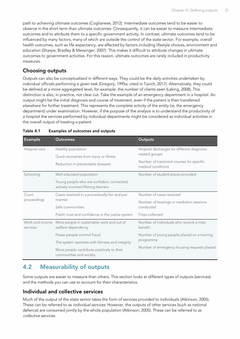
Chapter 4 | Defining outputs 21
path to achieving ultimate outcomes (Coglianese, 2012). Intermediate outcomes tend to be easier to
observe in the short term than ultimate outcomes. Consequently, it can be easier to measure intermediate
outcomes and to attribute them to a specific government activity. In contrast, ultimate outcomes tend to be
influenced by many factors, many of which are outside the control of the state sector. For example, overall
health outcomes, such as life expectancy, are affected by factors including lifestyle choices, environment and
education (Sharpe, Bradley & Messinger, 2007). This makes it difficult to attribute changes in ultimate
outcomes to government activities. For this reason, ultimate outcomes are rarely included in productivity
measures.
Choosing outputs
Outputs can also be conceptualised in different ways. They could be the daily activities undertaken by
individual officials performing a given task (Gregory, 1995a; cited in Tavich, 2017). Alternatively, they could
be defined at a more aggregated level, for example, the number of clients seen (Laking, 2008). This
distinction is also, in practice, not clear cut. Take the example of an emergency department in a hospital. An
output might be the initial diagnosis and course of treatment, even if the patient is then transferred
elsewhere for further treatment. This represents the complete activity of the entity (ie, the emergency
department) under examination. However, if the purpose of the analysis is to understand the productivity of
a hospital the services performed by individual departments might be considered as individual activities in
the overall output of treating a patient.
Table 4.1 Examples of outcomes and outputs
Example Outcomes Outputs
Hospital care Healthy population
Quick recoveries from injury or illness
Reduction in preventable diseases
Hospital discharges for different diagnosis-
related groups
Number of treatment courses for specific
medical conditions
Schooling Well-educated population
Young people who are confident, connected,
actively involved lifelong learners
Number of student places provided
Court
proceedings
Cases resolved in a procedurally fair and just
manner
Safe communities
Public trust and confidence in the justice system
Number of cases resolved
Number of hearings or mediation sessions
conducted
Fines collected
Work and income
services
More people in sustainable work and out of
welfare dependency
Fewer people commit fraud
The system operates with fairness and integrity
More people contribute positively to their
communities and society
Number of individuals who receive a main
benefit
Number of young people placed on a training
programme
Number of emergency housing requests placed
4.2 Measurability of outputs
Some outputs are easier to measure than others. This section looks at different types of outputs (services)
and the methods you can use to account for their characteristics.
Individual and collective services
Much of the output of the state sector takes the form of services provided to individuals (Atkinson, 2005).
These can be referred to as individual services. However, the outputs of other services (such as national
defence) are consumed jointly by the whole population (Atkinson, 2005). These can be referred to as
collective services.

22 Improving state sector productivity
This guide focuses on individual services. For collective services or particular services with both individual
and collective features, there are three main approaches for measuring their outputs:
Assuming the productivity growth of collective services is equal to that of similar services provided by the
private sector. For example, it could be possible to assume the productivity of public health campaigns
is equal to comparable campaigns in the measured health services.
Applying direct output measures where possible and reverting to an input method for the remaining
collective services. In effect, this means that collectively consumed services are excluded from the
productivity measure.
Measuring outputs where possible and using activity indicators for collectively consumed services. For
example, in the case of fire prevention services the total number of hours spent delivering prevention
activities might be an appropriate substitute for outputs (Office of the Deputy Prime Minister (UK), 2005).
Transactional and variable services
It is also possible to distinguish between transactional services and variable services. Outputs from
transactional services tend to:
be standardised, high volume and repetitive;
entail relatively little interaction with, or involvement of, consumers; and
be relatively easy to specify in advance; and
have relatively easy measurement of actual performance (OECD, 2001b).
An example of a transactional service is the payment of income-tested benefits. Transactional outputs are
generally relatively straightforward to measure. They are usually supported by comprehensive procedure
guides and operating manuals, which detail rules to be followed and standards to be met during the
production process (OECD, 2001b). Dunleavy and Carrera (2013) suggested that quality can be assumed to
be relatively constant for these types of outputs. They recommend that researchers take note of any
substantive failures of quality control when presenting productivity data, rather than seeking to quality adjust
the output numbers.
Variable services include teaching and individual health care. For these services outputs can be defined and
counted but they are subject to much greater variation than transactional services. Variable services are
often delivered with a high degree of interaction with, or involvement of, the consumer of the service. The
variability in production process introduces much greater scope for differences in quality. This makes quality
adjustment (discussed in Chapter 6) more important.
4.3 Coverage of outputs
Ideally, the range of outputs included in productivity measures would be comprehensive (Statistics
New Zealand, 2010). Including a subset of outputs may lead to a misleading picture of changes in
performance and/or encourage state-sector agencies to focus on measured outputs at the expense of
unmeasured ones (Simpson, 2009). The New Zealand Council of Trade Unions raised this concern:
Elevating any subset of measured outputs to ‘core’ status [….] risks distorting the operations of the
organisation or programme if more effort is devoted to improving that indicator at the expense of its
complete set of objectives (sub. 9, p.6).
Yet a principle that always required complete coverage of outputs would be impractical. There may be gaps
in data availability. In practice, a balance is needed between coverage and the cost of a measurement
(Atkinson, 2005).
There may also be diminishing marginal returns from attempting to measure all outputs. As one submitter
noted:
Chapter 4 | Defining outputs 23
It is neither necessary nor desirable to measure every single output of any sector, service or function.
The Pareto principle states that, for a lot of events, roughly 80% of effects come from 20% of the causes
… This 80/20 rule can be applied in this context by focusing on the critical 20% of functions of any sector
which would produce roughly 80% of the outputs. This would maximise the cost/benefit ratio for the
project, deliver the most gains in productivity, and avoid wasting time dealing with problems which are
trivial (Hermann Grobler, sub. 5, p.6).
Statistics New Zealand (2010) suggested that if comprehensive coverage is not possible then the next best
option could be to aim for representativeness. In this case, it is necessary to identify outputs whose growth
rates can reasonably be assumed to be representative of growth rates for outputs where data is not available
or is costly to collect.
Other authors noted the importance of capturing the fundamental goods and services produced by the
agency in measures (SSC & Treasury, 2008; Dunleavy & Carrera, 2013). Dunleavy and Carrera (2013)
suggested asking (about a state sector agency) “what its broad mission is, and what few main outputs
capture that mission and can be cost-weighted in a reasonably accurate manner” (p.36). This approach
effectively measures productivity for these priority outputs and then, if an aggregate measure for an agency
is required, assumes the productivity of other outputs grows in line with growth in inputs. Note that in
developing this aggregate measure it is necessary to also estimate what share of total output is being
measured, what share is not being measured and whether this changes over time. For example, if a specific
output is used as a proxy for total output, then the calculation of aggregate productivity needs to consider
whether this output changes in importance to the agency over time. This is discussed in more detail in the
section on cost weighting in Chapter 5.
This guide emphasises defining outputs according to the availability of data and the ease with which any
additional data might be gathered. Statistics New Zealand (2010) noted that output coverage is typically
based on what information and classifications are already available, rather than on purity of concept.
However, it is important to not only measure what can be easily measured (Atkinson, 2005). While there are
practical constraints on what can be measured it is important to not lose sight of the central question
(understanding the services provided to households and firms). As he wrote:
… the procedure of defining direct output indicators within a government function should start by
seeking to identify the services provided by government to households and firms, and attempts made to
find data to reflect these services as comprehensively as possible, with appropriate allowance for quality
change. The services should be the starting point, not the available indicators (Atkinson, 2005, p.47).
This should not be taken as meaning the absence of complete data necessarily prohibits measurement
efforts. Instead, it simply means the limitations associated with measures should be clearly articulated and
efforts to improve the availability of data should be undertaken in parallel with measurement efforts.

24 Improving state sector productivity
Chapter 4 takeaways
In practice, distinguishing activities and outputs can be difficult and will depend on the purpose of
the analysis and the level at which the analysis is framed (service level, sector level, agency level,
etc.).
The output of collective services can be difficult to measure. In some cases, it may be possible to
assume productivity of these services has grown at the same rate as a similar (measurable) service
or by employing the “inputs equals outcomes” convention.
Transactional services tend to be highly standardised. For these services it may be reasonable to
assume quality is constant through time.
The production of variable services is less standardised. There is, therefore, more scope for
changes in service quality through time (see Chapter 6).
Ideally a productivity measure would include all outputs. However, this may be impractical and so a
“second-best” approach is to aim for representativeness. The outputs selected should capture the
core functions or mission of the entity.
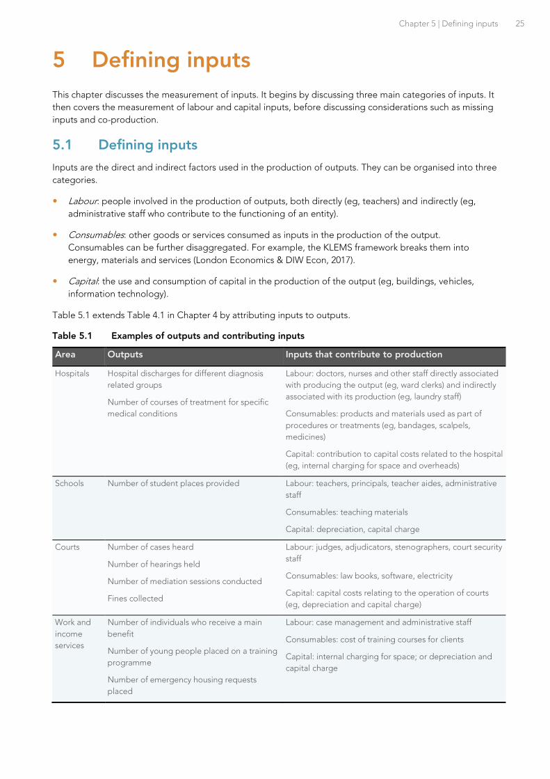
Chapter 5 | Defining inputs 25
5 Defining inputs
This chapter discusses the measurement of inputs. It begins by discussing three main categories of inputs. It
then covers the measurement of labour and capital inputs, before discussing considerations such as missing
inputs and co-production.
5.1 Defining inputs
Inputs are the direct and indirect factors used in the production of outputs. They can be organised into three
categories.
Labour: people involved in the production of outputs, both directly (eg, teachers) and indirectly (eg,
administrative staff who contribute to the functioning of an entity).
Consumables: other goods or services consumed as inputs in the production of the output.
Consumables can be further disaggregated. For example, the KLEMS framework breaks them into
energy, materials and services (London Economics & DIW Econ, 2017).
Capital: the use and consumption of capital in the production of the output (eg, buildings, vehicles,
information technology).
Table 5.1 extends Table 4.1 in Chapter 4 by attributing inputs to outputs.
Table 5.1 Examples of outputs and contributing inputs
Area Outputs Inputs that contribute to production
Hospitals Hospital discharges for different diagnosis
related groups
Number of courses of treatment for specific
medical conditions
Labour: doctors, nurses and other staff directly associated
with producing the output (eg, ward clerks) and indirectly
associated with its production (eg, laundry staff)
Consumables: products and materials used as part of
procedures or treatments (eg, bandages, scalpels,
medicines)
Capital: contribution to capital costs related to the hospital
(eg, internal charging for space and overheads)
Schools Number of student places provided Labour: teachers, principals, teacher aides, administrative
staff
Consumables: teaching materials
Capital: depreciation, capital charge
Courts Number of cases heard
Number of hearings held
Number of mediation sessions conducted
Fines collected
Labour: judges, adjudicators, stenographers, court security
staff
Consumables: law books, software, electricity
Capital: capital costs relating to the operation of courts
(eg, depreciation and capital charge)
Work and
income
services
Number of individuals who receive a main
benefit
Number of young people placed on a training
programme
Number of emergency housing requests
placed
Labour: case management and administrative staff
Consumables: cost of training courses for clients
Capital: internal charging for space; or depreciation and
capital charge

26 Improving state sector productivity
Differentiating between types of inputs is important when:
developing partial productivity measures, such as measures of labour productivity (see Box 1.1); or
decision-makers want to understand the impact of changes in particular inputs, such as the impact of
hiring more staff or buying new technology.3
Measures of multi-factor productivity (MFP) are useful when it is not possible to differentiate inputs into
labour, capital and consumables. MFP measures show the amount of output produced from each unit of
resource employed. The analysis includes all resources. Total expenditure can be used as a proxy for total
inputs (Gemmell, Nolan & Scobie, 2017b).
The inputs used in production can be calculated using a volume measure or an expenditure measure:
volume measures track changes in the number of inputs (eg, staff numbers, hours, or full-time
equivalents for labour); and
expenditure measures track changes in spending on the different types of inputs.
It is theoretically preferable to use volume measures in place of expenditure measures as they more directly
capture input changes (Atkinson, 2005). For example, a change in salary expenditure, even if adjusted for
inflation, reflects both changing hours of work (the volume of labour) and changes in wage rates (the price
per unit of labour). Yet in practice it will be unlikely that the volume of all inputs will be observable and so it
may be necessary to use some expenditure measures to ensure comprehensive coverage of inputs. Likewise,
in many cases the change in expenditure-based measures will be a reasonable proxy for changes in the
volume of inputs. Unless there are reasons for thinking that expenditure-based measures may be misleading,
the simpler approach of measuring inputs based on expenditure is generally recommended.
For cases where there is a need for a direct volume of inputs, the “Measuring labour volumes” section below
discusses approaches.
Measuring capital inputs
Capital refers to the fixed assets owned by the service provider and used in the production of outputs.
Buildings, computers and infrastructure are all examples of capital. Measuring capital can be difficult, as
discussed in Box 5.1.
The principle is to measure the flow of capital services. As Atkinson (2005, p.215) noted, for:
any given type of asset, there is a flow of productive services from the cumulative stock of past
investments. To illustrate, take the example of an office building. Service flows of an office building are
the protection against rain, the comfort and storage services that the building provides to personnel
during a given period… the appropriate measure of capital input for production and productivity
analysis is the flow of capital services of an asset type. This involves adding to the capital consumption
an interest charge, with an agreed interest rate, on the entire owned capital.
Dunleavy and Carrera (2013) suggested “a good proxy of capital consumption is capital depreciation, which
is published in most public organizations’ annual reports” (p.43). Depreciation measures reductions in the
value of the capital stock over the useful life of assets. Depreciation rates often vary, depending on the asset
in question and its expected useful life. These variations in depreciation rates are significant given the
growing use of digital technology in the state sector (Dunleavy, 2016).
3 Labour productivity measures the amount of output produced from each unit of labour employed, while capital productivity measures the amount of
output produced from each unit of capital employed.
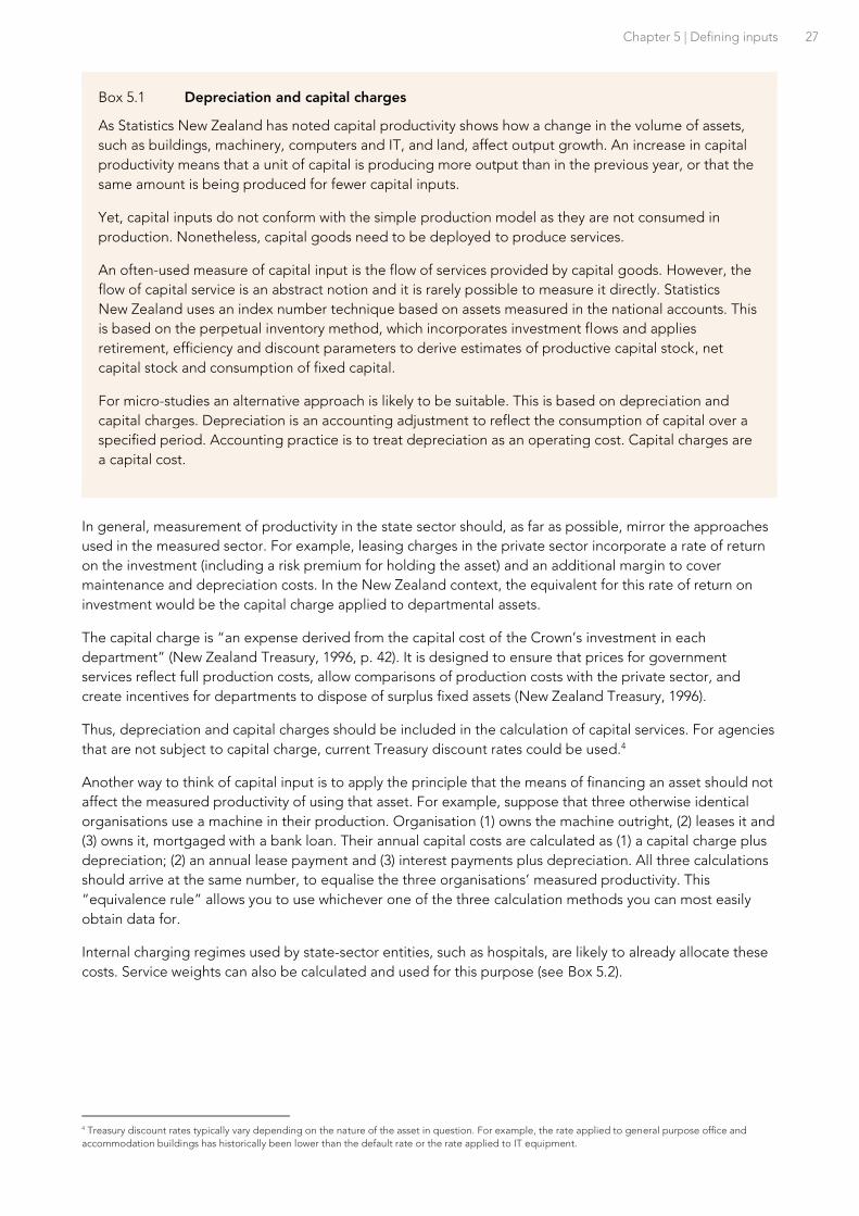
Chapter 5 | Defining inputs 27
In general, measurement of productivity in the state sector should, as far as possible, mirror the approaches
used in the measured sector. For example, leasing charges in the private sector incorporate a rate of return
on the investment (including a risk premium for holding the asset) and an additional margin to cover
maintenance and depreciation costs. In the New Zealand context, the equivalent for this rate of return on
investment would be the capital charge applied to departmental assets.
The capital charge is “an expense derived from the capital cost of the Crown’s investment in each
department” (New Zealand Treasury, 1996, p. 42). It is designed to ensure that prices for government
services reflect full production costs, allow comparisons of production costs with the private sector, and
create incentives for departments to dispose of surplus fixed assets (New Zealand Treasury, 1996).
Thus, depreciation and capital charges should be included in the calculation of capital services. For agencies
that are not subject to capital charge, current Treasury discount rates could be used.4
Another way to think of capital input is to apply the principle that the means of financing an asset should not
affect the measured productivity of using that asset. For example, suppose that three otherwise identical
organisations use a machine in their production. Organisation (1) owns the machine outright, (2) leases it and
(3) owns it, mortgaged with a bank loan. Their annual capital costs are calculated as (1) a capital charge plus
depreciation; (2) an annual lease payment and (3) interest payments plus depreciation. All three calculations
should arrive at the same number, to equalise the three organisations’ measured productivity. This
“equivalence rule” allows you to use whichever one of the three calculation methods you can most easily
obtain data for.
Internal charging regimes used by state-sector entities, such as hospitals, are likely to already allocate these
costs. Service weights can also be calculated and used for this purpose (see Box 5.2).
4 Treasury discount rates typically vary depending on the nature of the asset in question. For example, the rate applied to general purpose office and
accommodation buildings has historically been lower than the default rate or the rate applied to IT equipment.
Box 5.1 Depreciation and capital charges
As Statistics New Zealand has noted capital productivity shows how a change in the volume of assets,
such as buildings, machinery, computers and IT, and land, affect output growth. An increase in capital
productivity means that a unit of capital is producing more output than in the previous year, or that the
same amount is being produced for fewer capital inputs.
Yet, capital inputs do not conform with the simple production model as they are not consumed in
production. Nonetheless, capital goods need to be deployed to produce services.
An often-used measure of capital input is the flow of services provided by capital goods. However, the
flow of capital service is an abstract notion and it is rarely possible to measure it directly. Statistics
New Zealand uses an index number technique based on assets measured in the national accounts. This
is based on the perpetual inventory method, which incorporates investment flows and applies
retirement, efficiency and discount parameters to derive estimates of productive capital stock, net
capital stock and consumption of fixed capital.
For micro-studies an alternative approach is likely to be suitable. This is based on depreciation and
capital charges. Depreciation is an accounting adjustment to reflect the consumption of capital over a
specified period. Accounting practice is to treat depreciation as an operating cost. Capital charges are
a capital cost.

28 Improving state sector productivity
Measuring labour inputs
As noted above, unless there are reasons for thinking that expenditure-based measures may be misleading,
the simpler approach of measuring inputs based on expenditure is generally recommended. However, there
may be cases where there is a need for a direct volume of inputs. This section discusses approaches to
measuring labour volumes based on the Statistics New Zealand approach. The main approaches are
summarised in Table 5.2. The preferred measure of labour input is composition-adjusted hours of work. This
measure accounts for skill (often proxied by qualifications or years in work) differences among workers, so an
hour worked by a skilled person is given a greater weight than a less skilled person (Statistics New Zealand,
n.d.).
If the data needed for composition-adjusted labour measures are not available a “second-best” approach
can suffice. For example, in the Commission’s case study of early childhood education, the most detailed
data available were the number of full- and part-time teachers and their qualification status (Green, 2017).
For a more disaggregated measure of labour input the Commission:
weighted the part-time headcount numbers to distinguish their contribution to output production more
clearly (using a range of weights, from 0.25 to 0.75); and
used wage rates in the sector’s collective contract and Statistics New Zealand average income data for
early childhood teachers to weight the headcount numbers.
This allowed the labour input measure to reflect changes in the quality/composition of the teaching cohort
(Green, 2017).
The calculation of labour inputs should also account for the indirect costs associated with the production of
goods or services, such as labour provided through administrative or support services. Agency finance
divisions will have accounting rules for calculating or attributing the overhead contributions to outputs
(New Zealand Treasury, 1994).
Box 5.2 Using service weights when measuring the productivity of hospital services
District health boards use service weights to attribute spending to a specific service (eg, on an
operating theatre) when measuring productivity. Service weights enable them to calculate more
accurate efficiency and productivity measures for sub-outputs such as theatres, wards or radiology.
District health boards developed service weights as part of their health system performance
programme. They reflect the relative cost or input consumed by the outputs of a service. Conceptually,
they are same as output weights or cost weights. However, service weights relate to a specific service
while cost weights relate to an entire hospital.
For example, output weights should match the inputs consumed per output. For service components it
is necessary to include only those related to the service. When all costs are used they include some that
do not represent input into the production of the service. For example, in determining the efficiency of
theatres outputs should be weighted using theatre weights. These weights would reflect the inputs
consumed in theatre, not the resources consumed by the entire hospital.
Service weights can be developed in the same way as cost weights (eg, using actual cost information to
determine the relative cost of output). To produce cost weights the fully absorbed cost (entire hospital
cost) would be used, while service weights would use just the cost of the given service in the
production of outputs.
Source: District Health Boards, 2015.
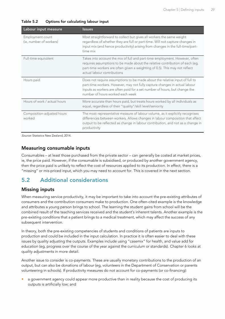
Chapter 5 | Defining inputs 29
Table 5.2 Options for calculating labour input
Labour input measure Issues
Employment count
(ie, number of workers)
Most straightforward to collect but gives all workers the same weight
regardless of whether they are full or part-time. Will not capture changes in
input mix (and hence productivity) arising from changes in the full-time/part-
time mix
Full-time equivalent Takes into account the mix of full and part-time employment. However, often
requires assumptions to be made about the relative contribution of each (eg,
part-time workers are often given a weighting of 0.5). This may not reflect
actual labour contributions
Hours paid Does not require assumptions to be made about the relative input of full to
part-time workers. However, may not fully capture changes in actual labour
inputs as workers are often paid for a set number of hours, but change the
number of hours worked each week
Hours of work / actual hours More accurate than hours paid, but treats hours worked by all individuals as
equal, regardless of their “quality”/skill level/seniority
Composition-adjusted hours
worked
The most representative measure of labour volume, as it explicitly recognises
differences between workers. Allows changes in labour composition that affect
output to be reflected as change in labour contribution, and not as a change in
productivity
Source: Statistics New Zealand, 2014.
Measuring consumable inputs
Consumables – at least those purchased from the private sector – can generally be costed at market prices,
ie, the price paid. However, if the consumable is subsidised, or produced by another government agency,
then the price paid is unlikely to reflect the cost of resources applied to its production. In effect, there is a
“missing” or mis-priced input, which you may need to account for. This is covered in the next section.
5.2 Additional considerations
Missing inputs
When measuring service productivity, it may be important to take into account the pre-existing attributes of
consumers and the contribution consumers make to production. One often-cited example is the knowledge
and attributes a young person brings to school. The learning the student gains from school will be the
combined result of the teaching services received and the student’s inherent talents. Another example is the
pre-existing conditions that a patient brings to a medical treatment, which may affect the success of any
subsequent intervention.
In theory, both the pre-existing competencies of students and conditions of patients are inputs to
production and could be included in the input calculation. In practice it is often easier to deal with these
issues by quality adjusting the outputs. Examples include using “casemix” for health, and value add for
education (eg, progress over the course of the year against the curriculum or standards). Chapter 6 looks at
quality adjustments in more detail.
Another issue to consider is co-payments. These are usually monetary contributions to the production of an
output, but can also be donations of labour (eg, volunteers in the Department of Conservation or parents
volunteering in schools). If productivity measures do not account for co-payments (or co-financing):
a government agency could appear more productive than in reality because the cost of producing its
outputs is artificially low; and

30 Improving state sector productivity
agencies may have an incentive to shift costs onto the public; for instance, by increasing the proportion
of costs covered by co-payments. By shifting costs, an agency may appear to be increasing productivity
without any real improvement in efficiency.
When studying the productivity of service, co-payments should be included as an input. However, if studying
the productivity of government funding only, then co-payments should not be included.
When other agencies’ outputs are the entity’s inputs
There is also a choice whether to use gross output or value-added measures. Value-added measures remove
consumables from gross output. Gross output measures are useful for understanding the total output of a
sector or organisation, while value-added measures are useful for assessing the marginal additional value
added. Statistics New Zealand (2010) illustrated this difference with a health sector example:
…if interest lies in understanding the marginal extra value added by the health system (for example, the
fact that medications are typically bought in and not produced by the government health sector, so are
not part of its value added), then a value added single or multifactor productivity methodology should
be constructed. If interest lies in understanding the total output of the health system, then a productivity
measure based on gross output should be constructed (p.19).
Chapter 5 takeaways
There are three types of inputs: labour, capital and consumables. Separating inputs into these
categories is important when seeking to understand how efficiently a specific input is being used
(eg, labour productivity) or what effect changes in an input have had.
It is theoretically preferable to use volume measures of inputs rather than expenditure measures,
but in practice it will be unlikely that the volume of all inputs will be observable. In many cases
changes in expenditure will be a reasonable proxy for volume changes. Unless there are reasons for
thinking that expenditure-based measures may be misleading, the simpler approach of measuring
inputs based on expenditure is recommended.
Include depreciation and interest or capital charges when estimating capital inputs (the
consumption of capital services). When measuring productivity at a service level it is important to
allocate capital inputs to particular services in proportion to the services’ consumption of those
inputs.
For cases where there is a need for a direct volume of labour inputs, composition-adjusted hours of
work is the preferred measure of labour. If composition-adjusted data are not available a simple
measure of labour will often suffice (eg, the number of hours of paid work).
Identify any relevant “missing inputs”, such as the pre-existing attributes of consumers. It may be
easier to account for such attributes through adjusting the quality of outputs (Chapter 6).
When assessing the productivity of a service, include co-payments. However, if assessing the
productivity of government funding only, you would exclude co-payments.

Chapter 6 | Cost weighting and price deflation 31
6 Cost weighting and price deflation
This chapter explains how to combine different outputs and inputs into single indexes. This is necessary
when measures cover more than just single outputs or inputs. The chapter also outlines how to account for
price changes.
6.1 Combining multiple outputs and inputs into single indexes
When measures cover multiple outputs or inputs they need to be combined into a single metric or index.
This can be a complex exercise. A simple count of the total number of outputs produced is unlikely to give
an accurate picture of how productive an entity is. Dunleavy (2016, pp.5-6) noted that for most private firms,
the presence of sales volumes and prices makes the process of calculating a total output metric relatively
straightforward.
… suppose a firm has two products, the first X priced at $5 and selling 20,000 units and the other Y
priced at $10 and selling 5,000 units. Its total output is thus: ($5 *20,000) + ($10 * 5,000) = $150,000. Price
is important here in two ways. First, it allows us to easily price-weight across completely dissimilar
products. Second, in competitive markets with consumer sovereignty, we can make welfare implications
about the sales patterns observed – in this case that consumers would not freely pay $10 for product Y
compared with $5 for product X unless they were getting commensurate benefits from it.
This approach is rarely feasible for the state sector because outputs are not priced, and many outputs must
be consumed whether citizens or enterprises wish to do so or not (Dunleavy, 2016; Gemmell, Nolan &
Scobie, 2017b).
Diewert (2017) suggests three methods for valuing state sector outputs, ranked in order of their desirability:
first best: valuation at market prices or purchaser’s valuations;
second best: valuations at producer’s unit costs of production; and
third best: output price growth is set equal to an index of input price growth.
The third-best method (assuming that inputs equal outputs) is a convenient way to overcome measurement
difficulties in the state sector. But, by definition, it will measure productivity growth as zero. So this method is
of little value. The following sections examine the advantages and disadvantages of Diewert’s first and
second-best approaches.
Valuation at market prices or purchaser’s valuations
One method for valuing outputs is to obtain price information from comparable services provided in the
private sector. Atkinson (2005) gave two examples:
In the case of road use, “we may attach value weights to passenger miles and to freight tonne miles,
based on the alternative costs of using rail” (p.89).
The provision of personal care by social services, where there is a parallel private market. The price that
people are willing to pay for daily care in the private sector can be used for the marginal valuation.
Simpson (2009, p.255) also noted that comparable prices in the private sector can be used to value state
sector services, but offered the following caveats:
… private sector alternatives might differ in their scope and characteristics; private healthcare might
offer reduced waiting times and higher quality accommodation. In addition the characteristics of
individuals using private sector alternatives, for example their underlying health, may differ from those
using public sector provision and may also affect the price. Hence in each case questions would remain
about how reliably these methods would capture the relative valuations of different goods.
32 Improving state sector productivity
In addition, the sheer size of the state sector as a provider of certain services (eg, health care) can skew the
price of parallel services provided in the private market. In other cases, (eg, police, fire service) there is no
comparable private market (Parker, Waller & Xu, 2013).
Willingness-to-pay (WTP) methodologies can also be used to estimate the value consumers place on
particular outputs. WTP approaches seek to establish in advance what somebody would be prepared to pay
to receive goods or services, for example, a particular health intervention. There are two broad approaches
for estimating WTP (Accent & RAND Europe, 2010):
Revealed preference methods observe people’s preferences indirectly; as revealed by actual market
behaviour and other choices they make. Examples include the premium that individuals are willing to pay
to live in the catchment area of particular schools, how long individuals are prepared to wait for a certain
service, or how far they are willing to travel to access a certain hospital (Simpson, 2009).
Stated preference methods ask people how much they would pay. In an environmental context this
might involve asking how much an individual would agree to pay for avoiding a degradation of the
environment or, alternatively, how much they would ask for as compensation for the degradation.
Alternatively, people can be asked to make trade-offs among different alternatives, from which their
willingness to pay can be estimated.
The New Zealand Initiative (sub. 8) supported the investigation of techniques for assessing the value of non-
market outputs including revealed preference methods. In particular, it noted the “risk-premium that obtains
for particular jobs, for example, can provide a reasonable benchmark for the value that workers place on
avoiding relatively small risks” (p.3).
Other submitters were less optimistic about WTP methods. For example, New Zealand Council of Trade
Unions (sub. 9) and the Public Service Association (sub. 14) argued that “public services are not market
goods and there is no value in a subjective measure based on the assumption that they could be treated as
such”.
While there can be benefits from using WTP methods, designing and executing a reliable approach requires
time and expertise. In many cases a weighting approach based on unit costs is likely to be sufficient.
Valuations at producer’s unit costs of production
The per-unit production costs method applies weightings to different outputs based on the cost of
providing that output. In doing so, these costs act as a proxy for the per-unit value to the service recipient. If
a state sector entity has three core outputs – A, B and C – output would be calculated using:
(units of A * unit costs for A) + (units of B * unit costs for B) + (units of C * unit costs for C)
(Dunleavy, 2016)
The use of market prices or purchaser valuations attempts to attribute societal value to public services. By
contrast, cost weights reflect willingness of governments to pay for public services. Box 6.1 and Box 6.2
provide examples of applying cost weightings in various measures of state sector productivity. Box 6.3
discusses the sensitivity of these measures to different approaches to cost weighting.

Chapter 6 | Cost weighting and price deflation 33
Box 6.1 Examples of cost weightings in state sector productivity measures
In their study of the evolution of productivity in the UK customs service, Dunleavy and Carrera
(2013) measured two outputs: the total numbers of import and export declarations processed per
year. These volumes were weighted by the relative unit costs in each year to create a total outputs
data series.
The Office for National Statistics (2012) calculated output of the UK education sector using the
number of students in nine different learning services, including schools, the higher education
training of teachers and health professionals and further education. Student numbers were
weighted by their share in aggregate education expenditure and converted into a single education
output series.
Administrative costs can be a useful proxy where reliable data on per-unit costs are not available. In
their study of productivity in UK tax administration, Dunleavy and Carrera (2013) used the share of
administration costs for different taxes collected to weight the different tax volumes. Weighted tax
volumes were added together to create a total index of tax output.
In an analysis of police productivity in England and Wales, Pritchard (2003) applied weightings to
categories of crimes investigated based on the costs involved. Results showed that although the
total number of recorded crimes reduced between 1995 and 2001, the weighted output of
investigations actually increased. This was due to a sharp increase in violent crime (which is the
costliest type of crime to investigate) and a reduction in several types of crime that are less
expensive (such as thefts from vehicles and burglaries).
Box 6.2 Combining police outputs related to mental health and attempted suicide incidents
The Commission worked with the New Zealand Police to produce productivity metrics for police
responses to mental health and attempted suicide incidents. Mental health-related calls received by
police have grown rapidly, increasing nearly tenfold from 5 000 in 1996 to 47 000 in 2017. In addition to
increasing in volume, the New Zealand Police has suggested that mental health incidents are becoming
increasingly complex.
Potential difficulties in measuring mental health and attempted suicide incidents were overcome using
case weights derived from administrative data. The police central dispatch system allocates tasks to
police officers and records staff activity information. Case numbers were calculated for mental health
and attempted suicide incidents. To account for differences in the complexity of incidence, cases were
weighted using the average time a police officer spends responding to each incident class. More
complex incidents require more police time.
The New Zealand Police is seeking to improve policing services for people with mental health
conditions. The study showed police officers spent not only more time on mental health incidents, but
more time on each incident over the seven years of the study.
The use of administrative data to derive weight and other information removes judgments and
potential sources of human error in constructing productivity metrics. However, careful attention needs
to be paid to ensuring the weights are sensible and are representative over time.
Source: Genet and Hayward, 2017.

34 Improving state sector productivity
6.2 Accounting for price changes
Productivity is a volume measure. Sometimes it is not possible to measure the volume of inputs and outputs
directly, and expenditure will need to serve as a proxy. Yet changes in expenditure can reflect changes in
volume, changes in prices, or both. For instance, a change in expenditure on staff could reflect changes in
the volume of labour (say the number of hours worked) and/or changes in salaries. As such, expenditure
figures need to be “adjusted” to account for price movements. This allows changes in volume to be
identified (Atkinson, 2005).
Consider a service where the direct volume of output cannot be measured and where input prices have
fallen over time, so it is now cheaper to provide the service. In this case, expenditure on the service could
remain the same while the volume of output increased. Failing to “deflate” input costs (ie, remove the effect
of price changes) would overstate any productivity improvements.
Crucially, the approach used to deflate expenditure can have a material impact on productivity estimates.
The following sections provide more detail on the selection and use of price deflators.
Characteristics of a good price deflator
Atkinson (2005) presents criteria for assessing the adequacy of price deflators (Table 6.1). The criteria cover:
the quality of the deflator (eg, comprehensive, full coverage);
the availability of data (eg, sustainability, timeliness, periodicity, availability of cost weights); and
the capacity of the deflator to illustrate the questions under consideration (eg, relevance, homogeneity
and quality change).
Box 6.3 Sensitivity of productivity estimates to cost weighting approaches
Gemmell, Nolan and Scobie (2017a) examined university productivity separately for teaching and
research. This required total staff FTEs and expenditures to be separately estimated for teaching and
research.
They recognised that academic staff in universities typically split their time between teaching, research
and administration, and so allocated non-academic (mainly academic support) staff FTEs to teaching
and research on a pro-rata basis. This led to a staff FTE split between teaching and research that on
average was around 40:60 in favour of research, over the period 2000 to 2015.
Similarly, they used income sources in universities’ published financial accounts to estimate
expenditure allocation between teaching and research, and allocated some government tuition and
student fee income to research to capture the fraction of time academic staff, funded from this income,
spend on research on average. This yielded a teaching/research expenditure allocation around 40:60
across all universities on average, similar to that of their first approach.
The authors also explored the impact of changing these assumptions on university productivity growth
estimates. To examine sensitivity they adopted the extreme alternative that all academic staff FTEs
were allocated to teaching, with research FTEs obtained from the “research staff FTE” category in
Ministry of Education data. Similarly, they treated tuition/student fee income as teaching related for the
purposes of expenditure allocation.
Overall, assuming a much more heavily weighted allocation of university resources towards teaching
suggested that productivity growth was substantially lower than it would appear with a more research-
weighted allocation. And, while quality-adjustment generally produced faster productivity growth than
basic measures, both those measures were lower with greater input allocation to teaching.
Source: Gemmell, Nolan and Scobie, 2017a.

Chapter 6 | Cost weighting and price deflation 35
Table 6.1 Quality criteria for price deflators
Criterion Description Examples and explanation
Comprehensiveness The set of deflators should cover all
components of expenditure to be deflated
There should be full geographic and sector
coverage of the expenditure being deflated
(eg, health deflators should cover the whole of
the health system not just hospitals)
Coverage The individual deflator should relate to all
expenditure on the item to be deflated
Deflators for labour expenditure should cover
all aspects of employee compensation (eg, all
direct taxes and social security contributions
and pensions as well as earnings)
Relevance The deflator should correspond to the
expenditure item to be deflated
For example, expenditure on books should be
deflated using an indicator of the price change
in books
Sustainability The deflator should be available for the
foreseeable future, and for a reasonable
number of periods in the past
Micro-studies of changes in price for only a
single year have limited use: long time series
are preferable
Homogeneity Deflation should be carried out at a level of
disaggregation that maximises
homogeneity of items within a category
For example, significant difference in the
movement of pay between staff grades would
suggest that separate deflators are needed
Timeliness The deflator should be available in good
time after the end of the reference period
Estimation for missing periods may introduce
bias
Periodicity The deflator should be available on a
quarterly basis
Annual figures may be satisfactory, but only
where there is evidence of insignificant short-
term change
Quality change Where changes in characteristics of a good
or service occur, price indexes should
reflect pure price changes only
Improvements in composition and
consequently effectiveness of a drug should
be distinguished from pure price change
Availability of cost
weights
Corresponding weights (of the same
periodicity) for deflators should also be
available
Source: Atkinson, 2005.
Calculating deflators
In some cases, market price information (such as the Consumer Price Index) can be used to deflate values of
non-market outputs (Schreyer, 2010). An alternative is to construct direct volume indexes. Different indexes
can be combined using fixed base or chain-weighted approaches.
Market price information
Where the data required to estimate direct volume indexes are not available, it may be possible to use
publicly available Statistics New Zealand deflators. Important sources of data from Statistics New Zealand
include the following.
Consumer Price Index (CPI): The CPI measures the changing price of a fixed basket of goods and
services. This basket is representative of the spending habits of New Zealand households and remains a
fixed quantity so that changes in the CPI represent only price changes. As the quantity must remain
fixed, Statistics New Zealand makes adjustments for any changes in the size, performance or functionality
of products. Every three years Statistics New Zealand reviews the basket of goods to account for
changes in household spending habits over time. The goods and services covered by the CPI are
classified into nine groups, 21 subgroups and 73 sections.
36 Improving state sector productivity
CPI subgroups: A number of the CPI groups and subgroups include data on public services (such as
primary and secondary education). These subgroups reflect consumers’ spending in these specific areas,
while the CPI reflects price movements more generally.
Purchasing Price Index (PPI): Another possible deflator is a subgroup of Statistics New Zealand’s PPI. This
index only covers the “productive sector” and measures changes in the prices of outputs that generate
operating income and of inputs that incur operating expense. It does not include prices for items related
to capitalised expenditure, non-operating income, financing costs or employee compensation. The
subgroups are not published at a further disaggregated level (eg, split into primary and secondary
schools).
When considering the use of market price information, it is necessary to check the data is suitable for
deflating non-market production (Schreyer, 2010). In particular:
the services supplied by market providers have to be sufficiently similar to those supplied by non-market
providers – this has to be true for each type of service and for the mix between different services; and
the deflator needs to reflect the full cost of production.
On the second point, some market information (such as the CPI) only reflects consumer’s out-of-pocket
expenditure. However, many public services are subsidised meaning the “out-of-pocket” price does not
reflect the costs of delivering the service. For example, in the CPI the price for medical services only reflects
patients’ out-of-pocket expenditure, yet these services are heavily subsidised by the state. Using CPI data for
medical services would therefore likely underestimate price changes.
For example, Gemmell, Nolan and Scobie (2017b) compared quality adjustments based on the full CPI with
those based on the CPI level 2 subgroup for primary and secondary education (reflects consumers’ spending
on schooling) (see Box 8.3). They argued for using the full CPI to deflate teacher salaries and school revenue.
The full CPI provides a “common numeraire” as the basis for all real comparisons, so it indicates a common
average real basket of goods that the funds in question could alternatively buy.
Direct volume indexes
A direct volume index is the weighted average of the volume indexes of different types of activity, where the
cost share of each type of activity constitutes the weight (Schreyer, 2010). There are several approaches to
producing direct volume indexes such as the Paasche and Laspeyres indexes (see Box 6.4).
Box 6.4 Three approaches to calculating direct volume indexes
The Paasche index calculates the expenditure needed to buy current year quantities. It is expressed
as a percentage of what the expenditure would have been in the base period if the quantity
consumed had been at current levels (Goodridge, 2007). It divides spending on a basket of goods
and services in the current period (ie, the sum of price multiplied by quantity for each product) by
how much the same basket would cost in a base period. More formally this can be expressed as:
(Σ(Ptn)*(Qtn))/(Σ(Pt0)*(Qtn))
where Ptn and Qtn are prices and quantities at time n, and Pt0 is the price in the base period.
The main feature of the Laspeyres index is that the weights used are taken from the base period.
This can be expressed formally as:
(Σ(Ptn)*(Qt0))/(Σ(Pt0)*(Qt0))
where Ptn is the price at time n, and Pt0 and Qt0 are the prices and quantities in the base period.
Source: Goodridge, 2007.

Chapter 6 | Cost weighting and price deflation 37
The choice between approaches largely depends on the availability of data and how volatile prices are likely
to be. The Laspeyres index holds base prices constant and the Paasche index uses current prices. The
Paasche index requires data that are more recent while the Laspeyres uses historic prices. As such, the
Laspeyres index is likely to be most useful.
Fixed base versus chain weighting
When dealing with multiple inputs and outputs, it is necessary to have a method for combining indexes.
Simply averaging the change in indexes could be misleading as the volumes of different goods are likely to
vary.
For example, consider an entity with two outputs – A and B – where one unit of A has the same value as one
unit of B. Assume that initial production is 1 000 units of A and 10 000 units of B, and over a year production
of A increases by 5% and production of B increases by 1%. Averaging the two growth rates would give a
result of 3% while the actual growth in output would only be 1.4% (from 11 000 to 11 150).
There are a number of ways to combine different indexes. One option is to use a fixed-base approach. This
approach implicitly assumes that the value shares of different goods do not change over time. However, this
assumption is flawed in cases where the relative importance of goods is prone to change. For this reason,
weights are often adjusted regularly (annually or every five years).
Chain-linking is an approach where the weights are adjusted annually. This simply means that for each
period, the base used is the weight from the previous period (Goodridge, 2007). Chain-linking has
advantages over a fixed-base approach:
new outputs can be added to the “basket” every year. If the index is non-chained, new items can only be
added to the base year;
because the comparison is with the previous year (rather than a base year), chain-linking makes it easier
to identify annual changes (such as changes in price or the quantity of outputs produced); and
chain-linking removes the substitution bias encountered when there are large shifts in both the weight
and in the actual variable being indexed (Goodridge, 2007).
The ability to chain-link depends on the timeliness of the data used for the weights. Further, if the relative
values of goods do not shift over time, then chain-linking is unlikely to provide additional useful information.
Notably, chain-linking affects Paasche and Laspeyres indexes differently. When applied to Paasche indexes,
chain-linking has the effect of reducing the index because growth is not calculated as a percentage of
expenditure in the base period but instead is backward-looking. This means substitution effects are less
pronounced when the index is chained together. By contrast, a chain-linked Laspeyres index would rise by a
greater amount than the standard Laspeyres.

38 Improving state sector productivity
Chapter 6 takeaways
In many cases it will be necessary to combine multiple outputs (or inputs) into a single metric or
index. For private sector outputs market prices can be used. Many state-sector outputs are
unpriced or subsidised, so a different approach is usually required.
The generally recommended approach is to use per-unit production cost as a way of weighting
(combining) different outputs. These weights, however, reflect the value producers put on services
rather than consumers’ valuations.
Another way to value outputs is to use willingness-to-pay (WTP) measures. While there can be
benefits from using WTP methods, designing and executing a reliable approach requires time and
expertise, and in many cases a weighting approach based on unit costs is likely to be sufficient.
Changes in expenditure can reflect changes in volumes, changes in prices, or both. As such,
expenditure figures need to be “adjusted” to account for price movements. The approach used to
“deflate” this expenditure can have a material impact on productivity results. The use of publicly
available deflators, particularly the full CPI, is generally recommended. The approach taken must be
transparent as it can have a major impact on results.

Chapter 7 | Accounting for differences in operating environments and quality changes 39
7 Accounting for differences in operating environments and quality changes
A raw measure of productivity – the ratio of inputs to outputs – is not particularly useful by itself: it is only
meaningful as part of a comparison (Statistics New Zealand, 2010). Comparisons can be made between:
the productivity levels or growth rates of different entities; or
the productivity growth rate of a particular entity over time.
In making comparisons it is important to account for differences in the operating environments of entities
and for changes in operating environments over time. For example, differences in the performance of
schools may reflect the socio-economic status of their students as well as the performance of their staff.
Failing to account for these differences could mean measures overstate the performance of staff in schools
that draw students from advantaged backgrounds.
The quality of services may also differ between organisations and over time. Productivity measures must
account for these differences as well. For example, suppose a hospital increases the quality of its care and as
a result readmissions fall. The fall in readmissions results in the number of patients treated increasing at a
slower rate than the hospital’s inputs. Without accounting for the change in the quality, productivity
measures would tell a story of falling productivity and would miss the hospital’s improved performance.
The following sections discuss approaches for accounting for these differences and for changes in quality.
7.1 Differences in operating environments
Differences that organisations face in their operating environments can be seen in the example of two
hospitals that produce the same number of operations for the same quantity of inputs. These hospitals may
appear to have equal productivity but if one is treating patients with more complex conditions then the value
it is adding is higher. It is therefore important to account for differences in the complexity of activity in
measuring the output of public services such as hospital care. Differences in operating environments that
can be useful to account for include:
the characteristics of the clients of the services (eg, age, socio-economic background, pre-existing status,
support networks);
the size and scope of the organisations (eg, whether hospitals have specialist units);
market structure (eg, presence of other suppliers or competitors); and
overall performance of the economy.
Approaches to accounting for these factors include:
measuring the outputs related to different population subgroups separately (segmenting the population)
and treating them as distinct outputs;
limiting the range of providers studied to those from similar environments; and
adjusting the volumes of outputs for differences in the operating environment (eg, severity of
treatments).

40 Improving state sector productivity
Te Puni Kōkiri noted that in measuring state sector productivity the Commission should
focus on population segmentation to help build a more constructive understanding of how the public
sector engages with and delivers benefits to Māori, recognising that Māori needs are often complex and
intergenerational (sub. DR27, p.1).
An example of segmenting a population is the Commission’s approach in distinguishing users of social
services depending on how they access the system and their reasons for doing so (see Box 7.1). Under this
approach the productivity of the services received by clients in the four quadrants would each be measured
separately. However, studying different population groups separately (or limiting the range of providers
studied) can limit the scope of the analysis, unless cost weighting or other methods are used to combine the
results for different quadrants. The segmentation of District Health Boards into peer groups (Box 7.2)
illustrates another approach.
Box 7.1 Segmenting a population: people interacting with the social services system
In More effective social services (NZPC, 2015) the Commission highlighted how clients access the social
services system in different ways and for different reasons. For some, their main interaction with the
system is through their local school or childcare centre. On occasions, they may need to visit their local
general practitioner or perhaps a hospital if the issue is more serious. For these people, coordinating
services to meet their needs is relatively straightforward and, in many cases, they prefer to coordinate
their own interactions with the social services system.
The Commission segmented service users according to the complexity of their needs and their capacity
to extract the services they need from the system. The Commission found it useful to group clients
under four headings:
people with relatively straightforward needs who require assistance to access services (quadrant A);
people with relatively straightforward needs who have the capacity to access services for
themselves (quadrant B);
people with complex needs who have the capacity to access services for themselves (quadrant C);
and
people with complex needs who require assistance to access services (quadrant D).
B. Self-referral C. Client as integrator
A. Cross-referral D. Navigator as integrator
Low High
Low
Clie
nt
cap
aci
ty
Complexity of client need
High

Chapter 7 | Accounting for differences in operating environments and quality changes 41
An example of adjusting the volumes of outputs for differences in the operating environment is casemix
adjustment in the health sector (Box 7.3). This approach accounts for the characteristics of patients and is
used to allow for comparisons across settings or time. Volumes can be adjusted for case severity, typically
using cost weights (Rouse & Swales, 2006). These weights group together treatments that are clinically
similar, consume similar quantities of resources and are likely to be similar in cost. Casemix adjustment can
be applied to productivity measures for other public services. See Appendix C for an example.
Box 7.2 Grouping district health boards into “peer” groups
The Hospital Quality and Productivity framework was established in 2009 and concluded in 2015. The
framework established a series of performance indicators that allowed comparisons between DHBs.
The ministerial review group that initiated the framework noted:
There is much to be gained by reducing the substantial gap between the best and worst
performers within and between hospitals. This requires an independent set of productivity
measures at the appropriate level that are credible, useful and make sense to those hospital
clinicians and managers who are best placed to make productivity improvements within the
hospital. (p.5)
DHBs were clustered into peer groups to enable comparison of performance. DHBs were grouped
based the New Zealand Role Delineation Model (NZRDM) which differentiated the degree of
complexity between services provided across District Health Boards.
Source: District Health Boards New Zealand (2010).
Box 7.3 The casemix system used in the health sector
Health sector analyses use the casemix system to account for differences in patients’ pre-existing
conditions.
The casemix system is the basis for 28–29% of District Health Board funding in New Zealand. The
system has two parts: a clinical coding classification used to group events; and a cost weighting system
applied to these groupings.
The first step is to turn patients’ clinical records into clinical codes. The clinical coding classification
contains almost 2000 codes and can indicate:
major diagnosis category;
medical, surgical, or other procedures; and
level(s) of complication(s).
Given the number of clinical codes, similar events with comparable resource use are assigned to
Diagnostic Related Groups (DRGs). They enable hospital production to be measured by linking the
characteristics of patients treated (hospital activity) and the resources used in treating their patients
(input costs).
Cost weights – termed Weighted Inlier Equivalent Separations (WIES) – are then assigned to events
based on the DRG group, with adjustments for length of stay. Different cost weights exist for inlier
events, low and high outliers, and same day and one day events.
WIES is the system developed by the State of Victoria for casemix funding public hospitals. A version of
WIES has been adapted for New Zealand use (WIESNZ) and is updated annually.
Source: Casemix Project Group, 2015.

42 Improving state sector productivity
7.2 Quality adjustment
Quality can have many dimensions, as consumers may value a wide range of characteristics when consuming
public services. Schreyer (2010) outlines three general approaches to adjusting for changes in the quality of
the output of public services.
Implicit quality adjustment (stratification): This approach groups outputs so that only products and
services of the same specification are compared (Schreyer, 2012).
Explicit adjustments: Explicit approaches to quality adjustment are based on measures that adjust
outputs for changes in outcomes. There are two broad approaches to explicit quality adjustment.
- Explicit adjustment (proximate outcomes): The first approach is based on a resulting change in status
directly attributable to the services received (Schreyer, 2012). In this case, quality adjustments could
be based on factors like examination scores or attainment levels for education outputs (O’Mahony &
Stevens, 2009) or the change in health status associated with an intervention (Schreyer, 2012).
- Explicit adjustment (ultimate outcomes): A second approach is based on a broader definition of
outcomes as “a state that consumers value, for example the health status without necessarily relating
the change in this state to the medical intervention” (Schreyer, 2012, p.259). In this case, quality
indicators could include the population’s education level, life expectancy or level of crime. Proxies
for these indicators have included future earnings as a measure of the underlying population’s
education level or prices of houses as a measure of school quality (Black, 1998; Cannon, Danielsen &
Harrison, 2015; Gibson & Boe-Gibson, 2014).
Further, as Gemmell, Nolan and Scobie (2017a; 2017b) illustrated, it is also possible to use similar techniques
to quality adjust the inputs (eg, staffing) into state sector production. Different approaches are illustrated
below with examples from the education and health sectors.
Examples of possible quality adjustments in education
In education, quality adjustments can relate to inputs (eg, teacher quality or pupil to staff ratios), proximate
outcomes (eg, performance in school inspections or student attainment) or final outcomes (eg, impact on
Box 7.4 Implicit adjustments for differences in operating environments
Moore and Hayward (2017) used the Ministry of Social Development’s (MSD) individual Cost Allocation
Model to develop productivity measures of benefit-related transactional services. The study implicitly
adjusted for the impact of the operating environment by selecting “applications” as the output metric.
While demographic and socio-economic factors can have a significant impact on the quantity of benefit
applications, selecting applications as an output metric implicitly incorporated such factors.
Adjustments for the operating environment are only relevant if external factors are not sufficiently
accounted for within any output metrics. Common adjustments include demographic and socio-
economic characteristics, regional differences and the economic cycle.
If the benefit-applications study selected the overall serviced population (or region) as an output
metric, then it would have been important to adjust for the operating environment. Such adjustments
could have included the demographic characteristics and socio-economic status of the population,
which may be reflected in variations in dependence on welfare services.
Adjustments for the operating environment are common in other sectors that consider impacts at a
population level, such as the health sector’s use of a population-based funding formula for the
allocation of resources. In such cases, it can be appropriate to incorporate the impact of the wider
operating environment through such adjustments or models.
Source: Moore and Hayward, 2017.

Chapter 7 | Accounting for differences in operating environments and quality changes 43
human capital or on house prices due to school zoning). Table 7.1 lists some approaches to quality adjusting
school data. For examples related to tertiary education see Gemmell, Nolan and Scobie (2017a).
A further issue in quality adjusting data for state sector productivity is the proportionality problem. This
arises when comparing indexes of quality with indexes of inputs and outputs. It is necessary to establish a
“factor of proportionality” between the change in quality scores and the change in output (Schreyer, 2010).
Quality-adjusted outputs will not necessarily reveal how much extra quality is valued by the service users.
Should, for example, a 5% increase in student test scores mean the value of school output should be 5%
higher? This consideration is especially important when comparing productivity outcomes across industries,
for example, whether a 10% increase in the quality of education is equivalent to a 10% increase in quality of
health care.
Table 7.1 Approaches to quality adjusting school data
Concept Variables Measures Challenges
Labour inputs
(resources used
in production)
Labour Labour force (employment
count, FTEs, hours paid,
actual hours worked,
quality adjusted hours)
Combining non-commensurate
inputs into an index
Informal inputs (such as student
attributes)
Total inputs
(resources used
in production)
Labour, capital,
consumables (eg, teaching
aids, electricity usage and
building maintenance)
Total real operating
allowances
Implicitly assumes expenditure
weights are appropriate
Proximate
outcomes
Acquisition of skills and
qualifications
Transfer or increase in
knowledge
Pupil based: pupil numbers
(hours vs. EFTS),
educational attainment
(milestones, credits,
degrees)
Teaching based: number
of lessons, class size,
school inspections
Combining non-commensurate
outputs into an index
Attribution (eg, informal inputs)
Accounting for teacher quality
Grade inflation
Teaching to the test
Final outcomes
(direct)
Human capital Additional lifetime
earnings
Lags and attribution to expected
earnings
Final outcomes
(indirect)
Social network Housing value approach Accounting for more general
neighbourhood effects
Source: Howell, 2016; cited in Gemmell, Nolan and Scobie, 2017b.
Examples of quality adjustments in health
Approaches to quality adjustment can also be illustrated with the case of health care. There is a sizeable
literature on applying quality improvement approaches to health care and researchers such as Professor
Martin Connor of the Centre for Health Innovation, Griffith University, have illustrated the potential of
hospital performance data.
Marshall (2009) noted that statistical approaches first developed in the manufacturing sector could support
quality and reliability in health care. When it comes to defining quality, as with education, it is possible to
think about inputs (eg, wage rates; the qualifications of clinicians), proximate outcomes (eg, variations in
care; quality and safety markers) and final outcomes (eg, patient experience data; measures of whether
people are being treated in the right setting). Table 7.2 summarises some approaches.

44 Improving state sector productivity
Table 7.2 Approaches to adjusting health sector data
Concept Variables Measures Challenges
Labour inputs
(resources used
in production)
Labour Labour force (employment
count, FTEs, hours paid, actual
hours worked, quality adjusted
hours (eg, based on wage rates
or qualifications))
Combining non-commensurate
inputs into an index
Informal inputs (such as patient
characteristics)
Total inputs
(resources used
in production)
Labour, capital,
consumables (eg,
electricity usage and
building maintenance)
Total real operating allowances Implicitly assumes expenditure
weights are appropriate
Proximate
outcomes
Avoidance of direct
harm
Avoidance of excessive
variation
Quality and safety markers
Atlas of Healthcare Variation
Whether markers based on
priority areas reflect system
performance more generally
How to define appropriate
variation
Final outcomes Direct Patient experience data Currently limited to adult
inpatients, but being extended
to primary health care
Final outcomes Indirect Changing population shares in
levels of chronic care
Sampling bias and attribution
issues
Other examples of quality adjustments
Atkinson (2005) noted that the output of prison services is often measured by numbers of nights spent in
prison by prisoners on remand, prisoners under sentence, non-criminal prisoners and prisoners in police
cells. But this failed to quality adjust for overcrowding, reoffending and achievements during incarceration
such as educational attainment or drug rehabilitation. It also failed to weight according to cost, for example,
high risk vs. low risk prisoners. Atkinson (2005) argued that overcrowded cells could be given a lower weight
in output, although developing a precise weight requires robust evidence of the extent of overcrowding or
the threshold at which it becomes a problem. Atkinson (2005) also noted similar concerns about the standard
approaches to measuring outputs in benefit administration (see Table 7.3).
Table 7.3 Approaches to adjusting data in other sectors
Sector Unadjusted output Limitations Possible quality
adjustments
Prisons Number of nights Fails to reflect overcrowding,
reoffending, rehabilitation and
prior risk
Proportion of
overcrowded cells
Benefit administration Raw activity numbers Fails to reflect whether recipients
receive a high-quality service
Measures of timeliness
and accuracy of payments
Source: Productivity Commission.
Pros and cons of different approaches to quality adjustment
The choice of how to account for quality changes can have a significant impact on estimates of productivity
growth. Work in New Zealand and Australia has shown how sensitive estimates of productivity can be to the
approach taken to control for the quality of inputs and outputs.
Gemmell, Nolan and Scobie (2017b) tested a range of quality adjustments to productivity estimates for
New Zealand schools based on sector level data. They found that although most adjustments provided a

Chapter 7 | Accounting for differences in operating environments and quality changes 45
broadly (though not completely) consistent picture of flat or declining productivity, in one case the
change of method led to the measured productivity trend reversing.
The Australian Productivity Commission (Lovell & Baker, 2005) developed experimental productivity
estimates for 10 government services drawing on data contained in the Report on Government Services.
They found that the estimates of productivity were sensitive to the approach taken to control for the
quality of inputs and of outputs.
In the UK, the Office for National Statistics (ONS) takes a case-by-case approach to quality adjustment. It
uses stratification of services (implicit adjustment) and explicit adjustments (based on the attributable
contribution of the activity to outcomes). The ONS found that the greater degree of subjectivity involved in
quality adjustment compared to volume measures, means a higher standard is needed for judging their use.
Gemmell, Nolan and Scobie (2017b) tested approaches to quality adjusting productivity estimates. They
advise caution in making quality adjustments to labour inputs given important caveats on the use of salaries
as a proxy for quality of inputs. This reflects the nature of state sector labour markets (eg, whether a change
in total salaries reflects quality or compositional changes). They also highlighted the importance of missing
inputs such as the previous performance of students (needed for measures of value added).
Likewise, they argued that approaches based on final outcomes (such as the impact of the education system
on earnings) raised attribution issues. They showed how the decline in measures based on ultimate
outcomes was likely to reflect changes, at least partly, in unemployment and real wage growth following the
Global Financial Crisis. Changes in these measures reflect differences in the economic context facing
different cohorts of school leavers, not just the performance of schools.
Gemmell, Nolan and Scobie (2017b) argued that explicit adjustments should be based on the attributable
contribution of the activity to intermediate outcomes (such as student performance in tests). This was similar
to the conclusion reached by the ONS. However, even in this case there can be scope for ambiguity. For
example, student performance can be measured against performance in domestic or international tests and,
in recent years, the performance of New Zealand students in domestic tests has contrasted markedly with
their performance in international ones.
While Gemmell, Nolan and Scobie (2017b) pointed to challenges in quality adjusting state sector
productivity measures, they did not support relying only on unadjusted measures. Instead they noted that
quality adjusted measures should be treated as one (albeit essential) element of a broader framework for the
assessment of performance. Measurement approaches should be reviewed and may change as data
availability and analytical techniques improve.

46 Improving state sector productivity
Chapter 7 takeaways
Productivity measures are only useful as part of a comparison. Typically, comparisons are made
between the productive level (or growth rates) of different organisations, or between the
productivity of a specific organisation at different times.
When making comparisons, it is important to account for differences in the operating environments
of organisations and for changes in operating environments over time. Differences to look for
include differences in client characteristics, the size and scope of organisations, and the structure of
the market the organisations operate in.
Segmenting organisations or clients into comparable groups is one way to deal with differences in
the operating environment. Population segmentation can help build understanding of how
agencies engage with and deliver services to important population groups, such as Māori and
Pacific peoples.
Adjusting outputs, say through a casemix approach, is another way to deal with differences in the
operating environment. It may also be possible to limit the comparison to organisations with similar
environments.
Comparisons also need to account for differences in the output quality – either between
organisations or over time. Three approaches are used to adjust for quality.
- Implicit quality adjustment or stratification. This approach groups outputs so that only products
and services of the same specification are compared.
- Explicit adjustments based on proximate outcomes. This approach adjusts outputs based on an
observable change that is directly attributable to the services. For instance, the output of a
school could be adjusted based on the examination scores of its students.
- Explicit adjustments based on ultimate outcomes. This approach adjusts outputs based on a
change that consumers value, but which is not necessarily attributable to the services. For
instance, the output of a hospital could be adjusted using national life expectancy data.
Productivity measures can be sensitive to the approach used to adjust for quality. No approach to
quality adjustment is flawless, all have pros and cons. However, it is possible to develop reasonable
proxies for quality that can enhance unadjusted measures.

Chapter 8 | Measuring and checking 47
8 Measuring and checking
This chapter pulls the guide together by discussing frequently used productivity measures. It also discusses
the value in triangulating (sense testing) results with the findings of other studies.
8.1 Recap: productivity measures
Multi-factor productivity
Productivity is a measure of the effectiveness of an entity at converting inputs into outputs. As an illustrative
example, assume a one output and one input. The entity’s productivity can be measured as Q/I, where Q is
the total volume of output and I is the total volume of input. As there is a single input, this is a multi-factor
(or total) productivity measure.
Partial productivity
Partial productivity measures are where only one production factor (labour, capital or consumables) is used
as the input measure. The most commonly used partial productivity measure is labour productivity, which is
the ratio of total output to the total labour input. By contrast, when all the factors of production (inputs) are
included in the calculation, multi-factor productivity measures are produced.
A partial productivity measure like labour productivity has some advantages. It can show the impact of
changes in one specific factor on overall productivity. They can also be easier to undertake, as the data
requirements are lower. And for services that are labour intensive, labour productivity may offer a reasonable
indication of overall productivity performance.
However, partial productivity measures also have some drawbacks. Substitution between different inputs
(eg, greater use of technology in the treatment of health conditions) can lead to productivity changes. This
substitution between factors is unlikely to be captured in a partial productivity measure (Box 1.1). Using a
partial measure for performance evaluation may encourage gaming or goal displacement.
Comparison across time
Both partial and multi-factor productivity ratios are most useful when tracked over time or compared across
entities. Tracking a measure over time can show increases and decreases in the productivity of an entity.
There are several ways of conceptualising productivity growth: growth in a productivity index, in outputs
compared with inputs, and in real revenues with real costs. For example, with an index approach productivity
growth between periods 1 (t1) and 2 (t2) equals (Qt2/It2)/(Qt1/It1), where Qt1 and Qt2 are the quantities at
periods 1 and 2 and It1 and It2 are the inputs in these periods.
Adjusting inputs and outputs
The next step is to account for the fact that there are likely to be multiple inputs and outputs. As discussed in
Chapter 6, one approach is to use cost weights, so labour productivity can be written as Q/wL and multi-
factor productivity as Q/(wL+rK+mM), where:
w is the cost of labour and L the volume of labour input, and together they make up expenditure on
labour;
r is the user cost of capital and K the capital input, and together they make up the flow of capital
services, which can be proxied by depreciation and capital charges (see Box 5.1); and
m the unit price of consumables and M volume of consumables and together they make up expenditure
on consumables.
Likewise, where there are two outputs (a and b), Q is equal to caQa + cbQb, where ca, pb, Qa, and Qb are the
costs and quantities of a and b. You should consider whether the weights should be fixed over time (using
constant or current prices) and, if fixed, for how long or over what periods (eg, completed business cycles)?

48 Improving state sector productivity
8.2 Benchmarking
Benchmarking refers to a performance comparison across different entities to find the best performers and
provide information to assist poor performers.
Benchmarking can be point in time or over a period.
Point in time benchmarking
In making comparisons across entities it is important to be careful when comparing productivity levels. Given
the difficulty in accurately establishing productivity levels, these comparisons should generally emphasise
variations in growth rates. This, however, requires time-series data.
Benchmarking across time
Comparisons in the productivity measures of different entities over time can show how relative performance
is changing.
Benchmarking techniques
Benchmarking techniques are based on the principle of measuring the performance of one organisation (or
part of organisation) against a standard. This can either be an absolute standard or relative to other
organisations. It can be used to:
assess performance;
identify where improvement may be needed;
identify other organisations with processes that result in superior performance (encouraging the diffusion
of these processes); and
illustrate whether improvement programmes have been successful.
There are three main approaches to benchmarking:
benchmarking standards: setting a standard of performance that an effective organisation could be
expected to achieve;
benchmarking results: comparing the performance of a number of entities that provide a similar service.
This can illustrate whether an entity is making effective use of its resources compared to other entities;
and
benchmarking processes: examining the processes that produce a particular output, with a view to
understanding reasons for variations in performance.
Frontier analysis
A relatively technical form of benchmarking is frontier analysis. This approach can explain whether relatively
poor performance of a sector is due to a lack of productivity growth among the best performing
organisations (the frontier), or best practices failing to diffuse throughout a sector (eg, from the best
performers to the worst). Yet frontier approaches can be relatively data and resource intensive. Gemmell,
Nolan and Scobie (2017b) identified the following general stages in a frontier analysis.
Define the entities – entities (sometimes referred to as “decision-making units” in this literature) are the
units of frontier analysis. An entity could be an individual, firm, state-sector agency (eg, a school or
hospital), region or country.
Calculate the efficiency frontier – the efficiency frontier (sometimes called the reference set) is made up
of entities whose input levels are the lowest for any given level of output; this becomes the set against
which the efficiency of all entities can be assessed. There are two broad approaches to estimating
frontiers: non-parametric and parametric (see Box 8.1).

Chapter 8 | Measuring and checking 49
Estimate the distance of entities to the efficiency frontier – each entity receives an efficiency score that is
determined by their performance relative to that of the best performers.
Further detail about frontier approaches can be found in Gemmell, Nolan and Scobie (2017b), SCRCSSP
(1997) and Gabbitas and Jeffs (2008).
Box 8.1 When to use non-parametric and parametric frontiers
There are two broad approaches to estimating frontiers: non-parametric and parametric.
Non-parametric approaches make no allowance for “random noise” such as measurement errors or
other random shocks. As a result, any observation falling within the frontier is treated as technically
inefficient. The most widely used non-parametric approach is data envelopment analysis (DEA).
Parametric approaches, on the other hand, do not attribute all of the observed differences between
entities to differences in technical efficiency, as they allow for measurement error and other random
noise. As a result, no entities necessarily need to lie on the efficiency frontier (Gabbitas & Jeffs, 2008). A
widely used parametric approach is stochastic frontier analysis (SFA).
Considerations that influence the choice of technique include the following.
Cases with less heterogeneous samples are more suited to DEA. SFA is better suited to more
heterogeneous samples. DEA is more sensitive to heterogeneity in the sample (influenced by
outliers) and will tend to give lower average efficiency scores although not consistently. The
regression approach of SFA gives less weight to outliers.
Cases where output supplied is subject to variable or unpredictable client demand are less suited
to DEA. Unpredictability of client demand can introduce a source of variance in outputs and
weaken the relationship between inputs and outputs. SFA is better suited to coping with
unpredictable demand.
Both methods can deal with cases where exogenous variables influence operating environments.
Where these variables could be an important consideration, a DEA approach to restrict the
comparison set (to entities with similar or less favourable operating environments) is likely to be less
suitable. Other DEA approaches or an SFA approach based on regression analysis would be better.
SFA requires the parameters of the production function and the random error term to be
estimated. DEA is more suitable for cases where these parameters cannot be feasibly estimated,
such as where there are a limited number of observations available for robust regression analysis.
Gemmell, Nolan & Scobie (2017b) provides further detail about DEA and SFA. SCRCSSP (1997) and
Gabbitas and Jeffs (2008) provide practical guidance on DEA and SFA respectively.
Source: Gemmell, Nolan and Scobie, 2017b.

50 Improving state sector productivity
8.3 Bringing it all together
Table 8.1 is a useful summary of productivity questions that an entity may have and how these might be
answered with different measurement techniques.
Table 8.1 Productivity questions and measurement techniques
Productivity question Measurement
technique
Data requirements Suggested
interpretation
Has the entity’s
productivity changed over
a given period?
MFP analysis over the
target period
The flow of total outputs
produced by the entity over
the target period
Proxies for any changes in
output quality during the
target period
The flow of total (aggregate)
inputs used over the target
period
Price deflator
Changes in MFP (ratio of
outputs to inputs) through
time reflect changes in the
productivity of the entity
Over a given period, has
the entity’s productivity in
using a specific input
changed?
Partial productivity
analysis over the target
period
(Common measures
are labour productivity
and capital
productivity)
The flow of the input used
over the target period
Proxies for any change in the
quality of the input during
the target period
The flow of total outputs
produced by the entity over
the target period
Proxys for any change in
output quality during the
target period
Price deflator
Partial productivity measures
show the impact of changes
in a specific input on overall
productivity. For instance,
capital productivity shows
the amount of output
generated per unit of capital
input over the target period
Are some entities more
productive than others?
What should an entity do
to improve its
performance?
Benchmarking,
comparing entities at
one point in time
If the aim is to understand
why some entities are more
productive than others, input
data should be
disaggregated into specific
input categories (labour,
capital etc).
Quality adjusted inputs and
outputs for all target entities
is required.
As required to calculate MFP
levels for each entity at each
time
Dispersion of MFP shows
how much room to improve
there is for those short of the
frontier
Benchmarking,
comparing entities
over a time period
As required to calculate MFP
and partial productivity for
each entity at each time
Partial productivity measures,
and changes over time,
provide information about
the drivers of better and
worse performance
Source: Productivity Commission.

Chapter 8 | Measuring and checking 51
8.4 Sense testing results
For any study it is important to sense test the results. Box 8.2 contains useful questions that can be asked of
any productivity study. Box 8.3 discusses the approach taken to sense testing a study that quality adjusted
data on school productivity.
Productivity measures are just one dimension of the performance of the state sector. When drawing
conclusions, you should consider what is driving observed changes in productivity and, if necessary, how
these results compare with other sources of evidence. Atkinson (2005) emphasised the need to supplement
productivity measures with independent evidence, what he called a process of “triangulation”. It can also be
useful to consider the following questions.
What impact did the chosen approach and methodology have on the results? For example, as Gemmell,
Nolan and Scobie (2017a) highlighted, measures of tertiary sector productivity are highly sensitive to
approaches for cost weighting teaching and research activities and deflating outputs for price
How might changes in data collections and funding arrangements affect the results? For example, if
revenue from non-government sources is not included in the measure of inputs then changes in these
revenue sources can impact on the results
Box 8.2 Useful questions to ask of any productivity study
These questions can be used as a checklist for your analyses, or in understanding the work of others.
Outputs: How comprehensive were the range of outputs? If a subset of outputs was used, are the
most important or representative outputs included? How were changes in quality and/or collective
services accounted for?
Inputs: Did the study measure partial or multi-factor productivity measure? Was it sensitive to
changes in input mix? If so, does this impact on the usefulness of the productivity measure?
Labour inputs: How were labour inputs measured (expenditure or volume approaches)? What is the
likely impact of this? Were outsourced or contracted labour inputs included in the productivity
measure?
Capital inputs: Did the study employ both depreciation and a capital charge? If the study considers
a specific service line, how was capital apportioned to particular outputs?
Missing inputs: Did the study account for the pre-existing attributes of clients, or any co-payments?
Cost weighting: How did the study weight (value) different inputs and outputs? If market prices
were used, does the study explore the similarities or differences between state sector services and
private sector services?
Price changes: Has the study accounted for price changes over time? Does the deflator used
display the characteristics of a good price deflator?

52 Improving state sector productivity
As well as the quantitative techniques emphasised in this guide, qualitative techniques can be valuable for
the purposes of triangulating (or sense testing) the results. For example, comparative satisfaction surveys can
indicate the value that users attribute to public services in different jurisdictions. However, Bouckaert and
van de Walle (2003) argued that criteria such as “trust” and “more satisfaction” do not necessarily imply
better quality. Indeed, Boyle (2006) showed that for 15 European countries there was only, for example, a
moderate association between expenditure per capita on public services and satisfaction with public
administration. Making country comparisons can be difficult given changes in relative prices in countries
(measured in purchasing power parities) and the composition of international datasets (eg, with lower-
income countries joining the OECD).
Box 8.3 Sense testing results for quality-adjusted school productivity
The following example of quality-adjusting school productivity illustrates the importance of sense
testing results. It also shows that international comparisons can be a useful source of supporting
evidence.
Gemmell, Nolan and Scobie (2017b) estimated a range of quality adjusted productivity measures for
New Zealand schools and discussed the benefits and risks of different approaches (eg, regarding
teacher salaries, students’ performance in tests, or impact on earnings).
Adjusting these data for quality changes was complex in practice. As an example, the Office for
National Statistics (ONS) in the United Kingdom had to revise its approach to quality adjusting
education quantity when practices regarding students sitting exams changed. This is significant as any
quality adjustment can make a substantial difference to measured productivity.
One issue in the New Zealand study was the choice of deflator for school revenue data and the salary
data to account for the effect of price changes. The choice of deflator has a material impact on results.
The authors thus tested a range of deflators, including the education and training subgroup of the CPI
rather than the full CPI. However, using the subgroup meant that salary-based measures would grow
faster than unadjusted productivity measures, even though the growth in total salaries (4.4% nominal,
or 2.1% real when deflated by the full CPI) had been much faster than the growth in teacher FTEs (1.2%)
or price growth more generally (the CPI at 2.2%). This deflator failed a sense test.
One series of results for schools in this work was benchmarked against a series produced by the ONS. It
is important to recognise that given differences in public policies, policy contexts and data availability it
is appropriate for there to be some small methodological differences in the approaches and findings
for the two countries. Yet similarities in the general magnitude and direction of effect from making
broadly similar quality adjustment (based on performance in domestic assessments) can be expected.
In both countries the unadjusted series show similar trends. They both show a downward shift over time
reflecting policy choices regarding smaller class sizes. Making a quality adjustment based on pupil
attainment leads to average labour productivity growth around zero in both countries between 1997
and 2014, although in New Zealand a higher proportion of students achieving NCEA level 2 or above is
reflected in stronger multi-factor productivity growth since 2005.
Source: Gemmell, Nolan and Scobie, 2017b; Office of National Statistics, 2012.

Chapter 8 | Measuring and checking 53
Chapter 8 takeaways
There are two types of productivity measures. Partial productivity is the ratio of total output to a
specific input (ie, labour, capital or consumables). Multi-factor (or total factor) productivity is the
ratio of total output to all inputs.
Both partial and multi-factor productivity ratios are most useful when tracked over time or
compared across entities. Tracking a measure over time can show increases and decreases in the
productivity of an organisation or part of an organisation.
Benchmarking techniques information on how well an entity is performing relative to the best
performers in the sector.
Comparing productivity measures of different organisations can show how relative performance is
changing. Yet, comparisons of the absolute level of productivity must be done with care. It is
preferable to compare productivity growth rates rather than the absolute level of productivity.
For any study it is important to sense test the results. When drawing conclusions you should
consider what is driving observed changes in productivity and, if necessary, how these results
compare with other sources of evidence.

54 Improving state sector productivity
Appendix A Worked example: case study on early childhood education
Green (2017) estimated the productivity of the early childhood education (ECE) sector in New Zealand using
publicly-available data. This appendix summarises features of the study to illustrate the steps involved in
defining and producing a productivity measure.
Establish the business case
The Productivity Commission wanted to illustrate concepts for its state sector productivity inquiry with case
studies. It identified early childhood education (ECE) as a possible topic. Previously the Commission had
looked at parts of the education industry (school and tertiary education) but not the ECE sector. The
Commission wanted a case study that drew only on publicly available data to illustrate how far these data
could be taken, and the pros and cons of different measurement approaches. The Commission did not
intend for this to be an ongoing exercise.
Develop a clear research question
The research questions developed were:
using publicly-available information, estimate the labour and multifactor productivity of the ECE sector;
and
discuss options for quality-adjusting ECE outputs.
The availability of data constrained the time period for the analysis. Green decided that the productivity
measures produced would be gross, so no allowance was needed for consumables or intermediate inputs.
As the research questions relate to the whole sector, Green did not need data disaggregated by provider.
Establish what data you need
The statistics page of the Ministry of Education’s Education Counts website provided most of the necessary
data. The data were divided into outputs (participation rates and hours), inputs (labour and financial inputs,
serving as a proxy for total inputs), and proxies for changes in quality of inputs (staff qualification levels and
pay rates).
The website included annual ECE census report, along with statistics on ECE participation, services, teaching
staff, finances and language use. These included:
• Participation data: statistics on children's participation in ECE including tables on prior participation
rates of children starting school, enrolments and average hours spent in ECE. The relevant worksheets
were: “Time Series Data: Enrolments in ECE (2000-2017)” and “Time Series Data: Hours of Participation
in ECE (2000-2017)”.
• Teaching staff data: the numbers and characteristics of ECE teachers. These came from the “Time Series
Data: Number of teaching staff by full-time/part time status (2011-2017)” worksheet. The methodology
for collecting these data changed in 2014 (with a change to the treatment of relievers and temporary
staff) and so the years prior to this were not strictly comparable with later years.
• Financing data: statistics on expenditure on ECE, including tables on government expenditure on ECE,
and tables on the Consumers Price Index for the fees charged by ECE services. Two worksheets were
identified as having useful information: “ECE Expenditure” (which provided annual data for 2001/02 to
2014/15) and “ECE Fees” (which provided quarterly data from March 2005 to March 2015).
Green noted that additional data would be required to undertake quality adjustment. He used data on
teacher registration status (from Education Counts), short-term ECE teaching reliever wage rates (from NZEI),
and mean and median salaries in the preschool education sector (from the LEED dataset on Statistics New
Zealand’s infoshare website).

Appendix A | Worked example: case study on early childhood education 55
Green collated these pieces of data into a single Excel workbook, with labelled tabs and data sources
(including internet addresses where available) and date of collation noted in each worksheet. This approach
is helpful as readers and reviewers are easily able to check original sources. It also makes it easier for
researchers to update calculations in future years or when new data is available.
Define and measure outputs
Outputs were defined as funded child hours by service type (“Child Hours”). These data were available for
2001/02 to 2014/15. Te kōhanga reo funded child hours were excluded from the analysis (as there were no
staff input numbers).
Define and measure inputs
Labour inputs were defined as weighted staff numbers (“Staff Numbers”). These data were available for full-
time and part-time teachers and for 2002 to 2015. Staff numbers were based on:
Part time staff numbers for home-based and teacher-led services multiplied by 0.5 to construct a
weighted teacher numbers index. Other weights (0.25 and 0.75) were tried to test the sensitivity of these
results to this assumption.
Playcentre adults numbers multiplied by their average weekly hours of duty, divided by 35 (to provide a
weekly fraction) and then added to the weighted teacher numbers figure.
The 2004/05 year was used as the starting point for the analysis of overall labour productivity, as this was the
first year for which there were staff data for the home-based sector.
Total government expenditure on ECE (“Govt Expenditure”) was used as a proxy for total inputs.
Convert diverse outputs and inputs into a consistent format
Neither Child Hours nor Staff Numbers needed to be adjusted to account for changes in price levels. The
effect of changes in price levels on Govt Expenditure, however, did need to be taken into account.
Expenditure was deflated by the full CPI to give a series of real Govt Expenditure. The formula for this was
(Govt Expendituren/CPIn) * CPIb
where Govt Expendituren was government expenditure in year n, CPIn was the CPI level in the year n and
CPIb was the CPI in the base (starting) year.
Standardise inputs and outputs
Changes in the composition of the teaching workforce (such as the proportion of teachers who are qualified
or registered) were treated as changes in the quality of inputs. To address this Staff Numbers was adjusted
by the share of teaching staff who were “qualified” versus “not qualified” (based on Education Counts data)
and the wage premium for qualified teachers (based on NZEI data).
This wage premium varied among qualification levels. A teacher with a Diploma of Teaching had a premium
of 3% over an unqualified teacher, while a teacher with a 3-year degree or higher had a 23% premium. As the
qualification levels of teachers was not known, Green modelled two different scenarios. One where all
qualified staff received the lowest premia and one where they received the highest. These two scenarios
provided a range for the effect these premia may have.
The formula for adjusting Staff Numbers was:
Adjusted Staff Numbers = ((Staff Numbers * % Staff Qualified) * (1 + Wage Premia)) +
(Staff Numbers * (1 - % Staff Qualified))
Measure
Based on the steps above, the measures developed were:
Unadjusted labour productivity: Child Hours/Staff Numbers. This grew by an annual average of 0.4%
between 2004/05 and 2012/13.

56 Improving state sector productivity
Unadjusted multifactor productivity: Child Hours/Real Govt Expenditure. This declined by an average of
3.4% from 2001/02 to 2014/15.
Adjusted labour productivity: Child Hours/Adjusted Staff Numbers. Between 2000/01 and 2012/13 this
measure was, on average, either flat or fell by an average of 2.8% per annum. These results for adjusted
labour productivity are shown in Figure A.1.
Figure A.1 Labour productivity in the teacher-led ECE sectors, adjusted for wage premia for
qualifications, 2001/02 – 2012/13
Source: Green, 2017.
Notes:
1. The weights make different assumptions about the characteristics of “qualified” teachers. “Q1” weight assumes entry level qualification and little-to-no teaching experience. “Q3 weight” assumes an advanced qualification. Labour productivity should fall within these two bounds.
Check
Green presented preliminary results to an internal workshop at the Commission, and then discussed them
with stakeholders, including the Ministry of Education. Care was taken when writing up the findings given the
potential for misunderstanding. The paper was upfront about the fact that the ability to assess productivity
change in early childhood education (ECE) was limited by incomplete or inconsistent data. This could be
improved with:
teaching staff data on a full-time equivalent or actual hours-worked basis, rather than simple headcounts;
and
data, in monetary terms, on average hourly parental financial contributions (to match the data available
average hourly government subsidy rates).
Finally, Green discussed the broader setting for the use of any measures and noted that “measures used for
quality adjustment should have a close causal and empirically-demonstrated link to early childhood activities,
be relevant to the entire sector, and avoid overlaps with other parts of the education system.”
880
900
920
940
960
980
1000
1020
1040
2001/02 2002/03 2003/04 2004/05 2005/06 2006/07 2007/08 2008/09 2009/10 2010/11 2011/12 2012/13
Q3 weight
Q1 weight

Appendix B | Worked example: case study on New Zealand Police 57
Appendix B Worked example: case study on New Zealand Police
Genet and Hayward (2017) estimated the productivity of police responses to mental health incidents in New
Zealand. The steps undertaken in this study are summarised below as an illustration of the process of
defining and producing a productivity measure.
Establish the business case
The Productivity Commission wanted to illustrate concepts for its state sector productivity inquiry with case
studies. The Commission engaged with the New Zealand Police who wanted to improve their understanding
of responses to mental health incidents. The number of calls for police assistance has been growing rapidly,
and the New Zealand Police wanted to improve policing services for people with mental health conditions.
The Commission was keen to publish a case study that used administrative data from within an organisation
to construct productivity measures.
Develop a clear research question
The research questions developed were:
how has the labour productivity of police responses to mental health and attempted suicide incidents
changed over time; and
are there regional differences in labour productivity in these responses?
Establish what data you need
Police collect a significant amount of data about the volume of different outputs and their corresponding
labour inputs. Staff hour information is derived from the Police central dispatch system, which allocates tasks
to police officers. This system records, with a relatively high level of accuracy, the time a police officer takes
in responding to a certain incident, and the time taken before the incident is “closed”. Where dispatch
information is not available, estimates of staff time are used for cost allocation.
Define and measure outputs
This case study focused on initial scene attendance relating to mental health and threatened or attempted
suicide incidents.5 Incidents are coded when a call is placed with Police dispatch and coded again at the
closure of the initial scene attendance. A mental health incident is coded as “1M” and a threatened or
attempted suicide is coded as “1X”. Incidents initially coded as 1M or 1X but closed under another coding
are classified as “Other” for the purposes of this case study.
Incident classification may change during scene attendance. Changes include:
Incidents that start as mental health (1M) or threatened or attempted suicide (1X) that are then closed as
“Other”. For example, an incident may be classified as a mental health incident by dispatch but could be
reclassified due to other circumstances (such as a crime that results in an arrest). This occurs for
approximately 15% of mental health and threatened or attempted suicide incidents.
Mental health incidents that are closed as threatened or attempted suicide or threatened or attempted
suicide incidents that are closed as mental health incidents (ie, they change classification between the
two). This occurs for less than five percent of mental health or threatened or attempted suicide incidents.
Incidents that were first classified into another category (“Other”) but end as a mental health or
threatened or attempted suicide incident. This occurs in 35 to 40% of all incidents that end as mental
health or threatened or attempted suicide.
5 Attempted suicide incidents where there is a fatality are coded separately in the police dispatch system. They are not included in this analysis.

58 Improving state sector productivity
Table B.1 shows trends in mental health and threatened or attempted suicide by Police District – the raw
volume output measure for this study. Incidents are opened or closed as mental health or threatened or
attempted suicide increased by 79% over the period 2010/11 to 2016/17. Much of this increase is due to a
doubling of threatened or attempted suicide incidents responded to by Police.
Table B.1 Total outputs (responses to mental health incidents), 2010/11–2016/17
2010/11 2011/12 2012/13 2013/14 2014/15 2015/16 2016/17 % change
Auckland City 1 316 1 262 1 709 1 750 1 677 1 829 2 205 68%
Bay of Plenty 1 251 1 371 1 644 1 985 2 063 2 108 2 383 90%
Canterbury 1 910 1 931 2 384 2 796 2 811 3 094 3 471 82%
Central 1 621 1 683 2 256 2 447 2 644 2 782 3 116 92%
Counties/Manukau 1 392 1 571 2 072 2 188 2 244 2 339 2 435 75%
Eastern 825 885 1 151 1 299 1 250 1 419 1 507 83%
Northland 566 541 697 726 822 946 970 71%
Southern 1 073 1 028 1 309 1 461 1 604 1 747 1 914 78%
Tasman 532 603 797 866 887 1 081 1 259 137%
Waikato 1 404 1 377 1 753 1 994 2 043 2 069 2 346 67%
Waitemata 1 465 1 576 1 964 2 223 2 203 2 472 2 777 90%
Wellington 2 034 2 181 2 606 3 039 2 918 3 233 3 240 59%
Total 15 389 16 009 20 342 22 774 23 166 25 119 27 623 79%
Source: Data supplied by the New Zealand Police.
Notes:
1. This dataset is a subset of the New Zealand Police’s total mental health demand and response.
Define and measure inputs
This study uses the number of Police hours responding to mental health and threatened and attempted
suicide incidents as an estimate of inputs. As capital and intermediate inputs are not captured, it is not a
complete reflection of inputs. However, labour hours provide a reasonable estimate for inputs because
policing is labour intensive, and most overheads are allocated proportionately to staff time.
Convert diverse inputs into a consistent format
The total hours include both dispatch time and frontline police time. Dispatch staff members are paid a
comparable amount to frontline staff members and hence no weighting has been applied to these hours. An
extension to this study could involve weighting hours by individual staff members’ salary, or by groups of
staff members, to better reflect the staff input costs incurred by the New Zealand Police.
Standardise outputs
The total number of incidents are weighted for the purposes of this study. This is because mental health and
threatened or attempted suicide incidents are not necessarily comparable and are increasing at different
rates. The weights are derived using the average number of hours spent on mental health and threatened or
attempted suicide incidents in the 2010/11 year. Weights are calculated for each combination of start and
end codes for incidents. The total output metric is derived by multiplying the total outputs for each category
by these weights.
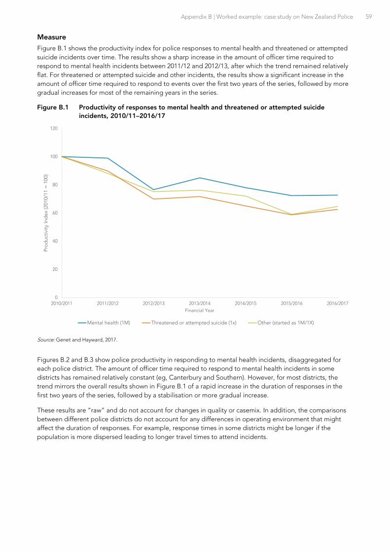
Appendix B | Worked example: case study on New Zealand Police 59
Measure
Figure B.1 shows the productivity index for police responses to mental health and threatened or attempted
suicide incidents over time. The results show a sharp increase in the amount of officer time required to
respond to mental health incidents between 2011/12 and 2012/13, after which the trend remained relatively
flat. For threatened or attempted suicide and other incidents, the results show a significant increase in the
amount of officer time required to respond to events over the first two years of the series, followed by more
gradual increases for most of the remaining years in the series.
Figure B.1 Productivity of responses to mental health and threatened or attempted suicide
incidents, 2010/11–2016/17
Source: Genet and Hayward, 2017.
Figures B.2 and B.3 show police productivity in responding to mental health incidents, disaggregated for
each police district. The amount of officer time required to respond to mental health incidents in some
districts has remained relatively constant (eg, Canterbury and Southern). However, for most districts, the
trend mirrors the overall results shown in Figure B.1 of a rapid increase in the duration of responses in the
first two years of the series, followed by a stabilisation or more gradual increase.
These results are “raw” and do not account for changes in quality or casemix. In addition, the comparisons
between different police districts do not account for any differences in operating environment that might
affect the duration of responses. For example, response times in some districts might be longer if the
population is more dispersed leading to longer travel times to attend incidents.
0
20
40
60
80
100
120
2010/2011 2011/2012 2012/2013 2013/2014 2014/2015 2015/2016 2016/2017
Pro
du
ctiv
ity
Ind
ex
(20
10
/11
= 1
00)
Financial Year
Mental health (1M) Threatened or attempted suicide (1x) Other (started as 1M/1X)
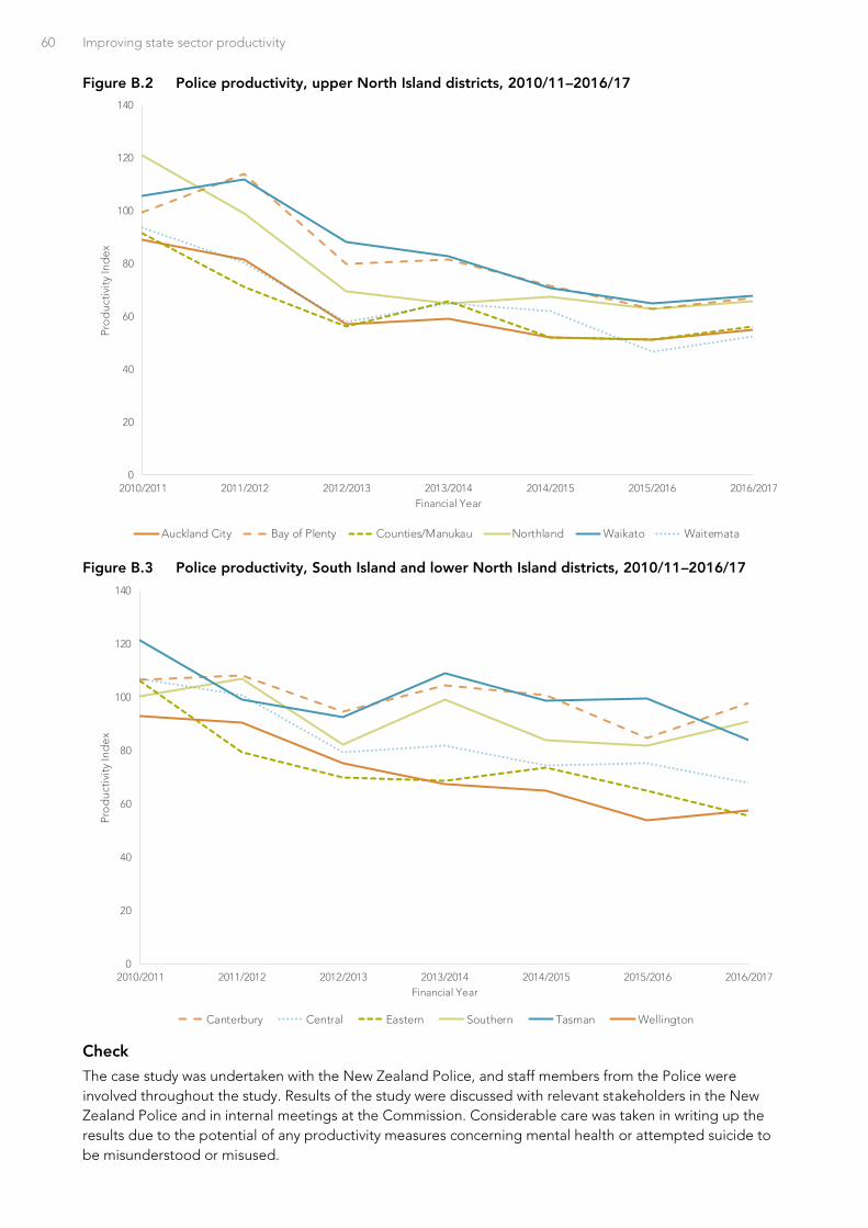
60 Improving state sector productivity
Figure B.2 Police productivity, upper North Island districts, 2010/11–2016/17
Figure B.3 Police productivity, South Island and lower North Island districts, 2010/11–2016/17
Check
The case study was undertaken with the New Zealand Police, and staff members from the Police were
involved throughout the study. Results of the study were discussed with relevant stakeholders in the New
Zealand Police and in internal meetings at the Commission. Considerable care was taken in writing up the
results due to the potential of any productivity measures concerning mental health or attempted suicide to
be misunderstood or misused.
0
20
40
60
80
100
120
140
2010/2011 2011/2012 2012/2013 2013/2014 2014/2015 2015/2016 2016/2017
Pro
du
cti
vity
In
de
x
Financial Year
Auckland City Bay of Plenty Counties/Manukau Northland Waikato Waitemata
0
20
40
60
80
100
120
140
2010/2011 2011/2012 2012/2013 2013/2014 2014/2015 2015/2016 2016/2017
Pro
du
cti
vity
Ind
ex
Financial Year
Canterbury Central Eastern Southern Tasman Wellington

Appendix B | Worked example: case study on New Zealand Police 61
The paper noted that the measures were “raw results”, and there are a number of factors that could impact
productivity performance that are not captured in the measure. Genet and Hayward (2017) noted the
analysis could be improved with adjustments for:
Quality – taking account of any changes in the quality of responses to mental health incidents. For
example, the amount of time police officers might be spending discussing the incident with the family of
the person suffering from mental health problems.
Case complexity – mental health incidents becoming increasingly complex and more challenging to
respond to, affecting the duration of responses.
Differences between districts in access to support services – no account is taken of the availability or
ease of access to District Health Board mental health services and how this may have changed over time.
This may affect how quickly Police are able to resolve an incident by transferring care to an appropriate
mental health service.

62 Improving state sector productivity
Appendix C Worked example: case study on universities
This guide is written from the perspective of an organisation that seeks to improve its own performance
through better understanding of its own productivity. However, the performance of public sector
organisations is of broader interest. Some public-sector entities have wide responsibilities to monitor various
aspects of the performance of other public entities. Examples include the Controller and Auditor-General,
the New Zealand Treasury and the State Services Commission. Others have narrower responsibilities,
including, for example, the Education Review Office (schools), the Ministry of Health (District Health Boards)
and the Productivity Commission (on inquiry topics as specified by Ministers). And public-sector entity
performance is, or should be, of concern to those who use and fund the services supplied.
The Controller and Auditor-General (2017) and NZPC (2017) inspired this example. Both studies sought to
understand how efficiently tertiary education institutions were using their physical assets. They relied on data
collected and published by the Tertiary Education Commission (TEC).
Establish the business case
Any visitor to a university is usually stuck by impressive buildings and the land they occupy. But are these
assets necessary for teaching? Or do they serve other purposes? Looking at a group of universities might
answer this question. The productivity measure of interest is the volume of teaching per unit of physical
capital. Should universities’ scores be closely bunched, then it is likely that they are efficient on this measure.
By contrast, significant dispersion might indicate the poor performers have significant room to improve.
For a single university, the business case lies in understanding its own performance relative to comparable
institutions, and the reasons why that may be the case. To the extent the underlying factors are under their
control, such understanding offers an opportunity to improve its performance.
For monitoring agencies, the business case revolves around understanding the wider application of public
resources. Information about productivity dispersion may inspire a change to policy, closer monitoring or
redirected funding that leads to better societal outcomes.
Develop a clear research question
The underlying question in both Controller and Auditor-General (2017) and NZPC (2017) is:
How does teaching capital productivity vary across New Zealand universities?
This case study demonstrates an iterative approach to answering this research question.
Establish what data you need
Answering this requires measurement of the capital productivity levels of each university on a consistent
basis, and then looking at the dispersion of those levels.
This example is intended to be illustrative rather than definitive. It is limited to publicly accessible data.
Conveniently, the TEC collates the annual audited data on the financial performance of all public tertiary
education institutions for comparative purposes. For simplicity of exposition, this example is limited to the
eight universities.
Define and measure outputs
The TEC dataset contains a teaching output measure – equivalent full-time students (EFTS). This measure
adjusts for part-time and part-year students. EFTS has known limitations as an output measure. However, it
(or its equivalent) is widely used for this purpose in New Zealand and internationally.

Appendix C | Worked example: case study on universities 63
Define and measure inputs
The TEC dataset also holds a convenient measure of physical capital stocks – property, plant and equipment
(PPE). Table C.1 reproduces the EFTS (output) and PPE (input) data.
Table C.1 Source data, EFTS and PPE for New Zealand universities, 2016
AUT Lincoln Massey Auckland Canterbury Otago Waikato VUW
Total EFTS 199 16 30 97 189 44 31 867 12 398 18 547 9 806 17 390
Property, plant &
equipment ($000)
773 626 186 183 1 048 451 2 432 637 1 046 794 1 539
646
409 107 794 828
Source: Spreadsheet published at http://www.tec.govt.nz/funding/funding-and-performance/performance/financial/. Accessed 19 July 2018.
Notes:
1. Property, plant & equipment is the average of the stocks at the end of 2015 and 2016. Other data is for the 2016 calendar year.
Convert diverse outputs and inputs into a consistent format
No conversion is required, since:
EFTS are a standardised measure, reflecting both teaching and student time; and
PPE values are measured in dollars.
No deflators were required, because this was a point-in-time comparison.
Measure
This example is iterative, and four productivity analyses are undertaken:
P1: unadjusted capital productivity: EFTS/PPE.
P2: research-adjusted capital stock productivity: EFTS/teaching capital.
P3: research-adjusted capital flow productivity: EFTS/teaching capital flows.
P4: casemix- and research-adjusted capital flow productivity: casemix-adjusted EFTS/teaching capital
flows.
Each step brings in any extra data it requires. All data comes from the same source. The first and second cuts
show the steps towards the analysis presented in NZPC (2017). Subsequent steps use the techniques
outlined in this guide to further refine the measure.
First cut: unadjusted capital productivity
Output: equivalent full-time students (EFTS)
Input: physical capital stock, as measured by PPE
Productivity measure 1 (P1): EFTS per thousand dollars of PPE.
Calculation: P1 = EFTS / PPE
For AUT: P1 = 19916 / 773626 = 0.026
This appendix shows the calculation steps for AUT only. Other ways of expressing this result include:
AUT requires one million dollars of physical capital to educate 26 full-time students; or
for each full-time student, AUT needs $38,500 of physical capital.

64 Improving state sector productivity
Table C.2 shows significant dispersion on the P1 measure. AUT is more than twice as productive as
Canterbury and Otago.
Table C.2 First cut: capital stock productivity, 2016
AUT Lincoln Massey Auckland Canterbury Otago Waikato VUW
EFTS per $000 PPE 0.026 0.017 0.018 0.013 0.012 0.012 0.024 0.022
A limitation
Universities produce more than just teaching. They devote much of their resources to research outputs. The
proportion of research to teaching varies across universities, so raw capital productivity may present
research-intensive universities unfairly.
Second cut: adjusting inputs to account for a second output
The TEC data do not include an output variable for research. However, the data does split university income
into teaching and research sources. The ratio of teaching income to the total of teaching and research
income is a weight that can be used as a proxy for the teaching intensity of the university. Table C.3 shows
the income data used to calculate this weight. ‘Teaching capital’ can be calculated using this teaching
weight to scale PPE.
Table C.3 University income data, 2016
($000) AUT Lincoln Massey Auckland Canterbury Otago Waikato VUW
Government tuition funding 146 937 28 462 153 067 329 375 125 478 230 530 72 645 137 762
Student fees & charges 168 174 23 873 169 570 286 356 101 603 164 504 81 862 134 950
Research income 27 804 41 706 103 347 332 567 59 775 171 347 50 424 79 438
There are some implicit assumptions in using current income data to scale a capital stock. One is that
research and teaching have a similar level of capital intensity. Another is that current income split has not
changed too much over time, as the capital stock reflects past decisions. Further research could test these
assumptions. This example assumes that these assumptions are reasonable.
Output: equivalent full-time students (EFTS)
Input: teaching capital (as calculated below)
Productivity measure 2 (P2): EFTS per thousand dollars of teaching capital
Calculation:
teaching weight = (Government tuition funding + Student fees & charges) /
(Government tuition funding + Student fees & charges + Research income)
teaching capital = PPE * teaching cost weight
P2 = EFTS / teaching capital
For AUT:
teaching weight = (146937+ 168174) / (146937+ 168174+ 27804) = 0.919
teaching capital = 773626 * 0.919 = 710899
P2 = 19916 / 710899 = 0.028

Appendix C | Worked example: case study on universities 65
Table C.4 shows P2 for the universities. The adjustment makes a significant difference for the research-
intensive universities, especially Lincoln and Auckland. P2 also has significant dispersion, with Waikato more
than twice as productive as Canterbury.
Table C.4 Second cut: research-adjusted capital stock productivity, 2016
AUT Lincoln Massey Auckland Canterbury Otago Waikato VUW
Teaching weight (%) 91.9% 55.7% 75.7% 64.9% 79.2% 69.7% 75.4% 77.4%
Teaching capital ($000) 710 899 103 613 794 089 1 579 514 828 663 1 073 858 308 445 615 531
EFTS per $000 teaching capital 0.028 0.030 0.024 0.020 0.015 0.017 0.032 0.028
A further limitation
Not all property, plant and equipment is equal. In particular, it gets depleted at different rates over time.
Accountants call this depletion as ‘depreciation’ and use different rates of depreciation for different classes
of assets. Should the makeup of PPE vary significantly between universities then a failure to include
depreciation could make universities whose assets are depreciating more quickly than those of their peers
appear more productive.
Third cut: using capital flows rather than stocks
Chapter 5 explains that you should use flows for capital inputs. One way to calculate capital flows is to add
depreciation and a capital charge. Depreciation is already in the financial dataset (Table C.5).
Table C.5 University depreciation, 2016
AUT Lincoln Massey Auckland Canterbury Otago Waikato VUW
Depreciation ($000) 38 931 7 721 49 560 115 141 44 588 57 883 21 512 41 384
For historical and political reasons, the government does not impose a capital charge on universities. The
rate that applied to other state sector entities in 2016 was 7%. This rate is a reasonable choice for this
analysis.
You should use the same capital charge rate for every entity in a cross-entity comparison, otherwise the
differences in rate could cause differences in measured productivity.
Output: equivalent full-time students (EFTS)
Input: teaching capital flow (as calculated below)
Productivity measure 3 (P3): EFTS per $000 of teaching capital flow
Calculation:
teaching capital flow = teaching capital * capital charge rate + depreciation
P3 = EFTS / teaching capital flow
For AUT:
teaching capital flow = 710899 * 0.07 + 38931 = 88694
P3 = 19916 / 88694 = 0.22
Table C.6 shows P3 for the universities. This adjustment made little difference to the relative rankings of the
universities.
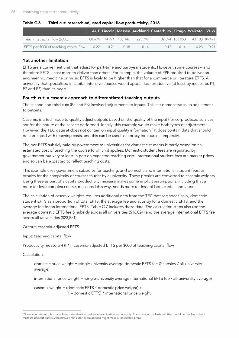
66 Improving state sector productivity
Table C.6 Third cut: research-adjusted capital flow productivity, 2016
AUT Lincoln Massey Auckland Canterbury Otago Waikato VUW
Teaching capital flow ($000) 88 694 14 974 105 146 225 707 102 594 133 053 43 103 84 471
EFTS per $000 of teaching capital flow 0.22 0.21 0.18 0.14 0.12 0.14 0.23 0.21
Yet another limitation
EFTS are a convenient unit that adjust for part-time and part-year students. However, some courses – and
therefore EFTS – cost more to deliver than others. For example, the volume of PPE required to deliver an
engineering, medicine or music EFTS is likely to be higher than that for a commerce or literature ETFS. A
university that specialised in capital-intensive courses would appear less productive (at least by measures P1,
P2 and P3) than its peers.
Fourth cut: a casemix approach to differentiated teaching outputs
The second and third cuts (P2 and P3) involved adjustments to inputs. This cut demonstrates an adjustment
to outputs.
Casemix is a technique to quality adjust outputs based on the quality of the input (for co-produced services)
and/or the nature of the service performed. Ideally, this example would make both types of adjustments.
However, the TEC dataset does not contain on input quality information.6 It does contain data that should
be correlated with teaching costs, and this can be used as a proxy for course complexity.
The per-EFTS subsidy paid by government to universities for domestic students is partly based on an
estimated cost of teaching the course to which it applies. Domestic student fees are regulated by
government but vary at least in part on expected teaching cost. International student fees are market prices
and so can be expected to reflect teaching costs.
This example uses government subsidies for teaching, and domestic and international student fees, as
proxies for the complexity of courses taught by a university. These proxies are converted to casemix weights.
Using these as part of a capital productivity measure makes some implicit assumptions, including that a
more (or less) complex course, measured this way, needs more (or less) of both capital and labour.
The calculation of casemix weights requires additional data from the TEC dataset; specifically, domestic
student EFTS as a proportion of total EFTS, the average fee and subsidy for a domestic EFTS, and the
average fee for an international EFTS. Table C.7 includes these data. The calculation steps also use the
average domestic EFTS fee & subsidy across all universities ($16,024) and the average international EFTS fee
across all universities ($23,851).
Output: casemix-adjusted EFTS
Input: teaching capital flow
Productivity measure 4 (P4): casemix-adjusted EFTS per $000 of teaching capital flow
Calculation:
domestic price weight = (single-university average domestic EFTS fee & subsidy / all-university
average)
international price weight = (single-university average international EFTS fee / all-university average)
casemix weight = (domestic EFTS * domestic price weight) +
(1 – domestic EFTS) * international price weight
6 Some countries (eg, Australia) have a standardized entrance examination for university. The scores of students admitted could be used as a direct
measure of input quality. Alternatively, the cutoff score applied might make a reasonable proxy.

Appendix C | Worked example: case study on universities 67
casemix-adjusted EFTS = EFTS * casemix weight
P4 = casemix-adjusted EFTS / teaching capital flow
For AUT:
domestic price weight = (13753 / 16024) = 0.86
international price weight = (23632 / 23851) = 0.99
casemix weight = (0.845 * 0.86) + (1 – 0.845) * 0.99 = 0.88
casemix-adjusted EFTS = 19916 * 0.88 = 17526
P4 = 17526 / 88694 = 0.20
Table C.7 shows the P4 calculations.
Table C.7 Fourth cut: casemix- and research-adjusted capital flow productivity, 2016
AUT Lincoln Massey Auckland Canterbury Otago Waikato VUW
Domestic EFTS (%) 84.5% 80.1% 85.0% 87.6% 91.1% 91.7% 84.6% 90.3%
Av. domestic student fee & subsidy ($) 13 753 15 301 15 539 18 046 16 835 19 962 14 408 14 349
Domestic price weight 0.86 0.95 0.97 1.13 1.05 1.25 0.90 0.90
Av. international student fee ($) 23 632 21 397 22 575 28 369 25 078 28 591 20 585 20 583
International price weight 0.99 0.90 0.95 1.19 1.05 1.20 0.86 0.86
Casemix weight 0.88 0.94 0.97 1.13 1.05 1.24 0.89 0.89
Casemix-adjusted EFTS per $000
of teaching capital flow
0.20 0.20 0.17 0.16 0.13 0.17 0.20 0.18
Auckland (with a medical school) and Otago (with medical and dentistry schools) get the highest casemix
weight. Canterbury (with engineering) comes next. Casemix weighting narrows, but does not eliminate, the
capital productivity dispersion. Canterbury remains the poorest performer. AUT, Lincoln and Waikato remain
the highest performers.
Check
There are many ways to further refine and improve this analysis, including the following:
Universities may lease physical assets for teaching purposes, in addition to the assets they own. The
capital input measure should ideally treat leased assets on an equivalent basis to owned assets. You
should add rents and leases paid to capital flows. For consistency, you should also add rates and other
costs of owning assets to capital flows.7
Apparently poor performance in capital productivity may reflect different ratios of capital to other inputs
(labour and/or consumables), rather than poor overall performance. A problem identified through study
of a partial measure should spur deeper and wider investigation.
The TEC dataset includes labour, measured in full-time equivalents, split into teaching and research
inputs. You could calculate a labour productivity measure using this data.
Interested readers should consult Gemmell, Nolan and Scobie (2017). It provides an extensive analysis of
quality adjusted productivity of New Zealand tertiary education providers.
7 Should a university lease out assets it owns, then rent and lease income should be subtracted from capital flows. Rates etc. for these assets should be
excluded from capital flows.
68 Improving state sector productivity
References
Accent & RAND Europe. (2010). Review of Stated Preference and Willingness to Pay Methods. Retrieved 13
September 2017 from http://webarchive.nationalarchives.gov.uk/+/http:/www.competition-
commission.org.uk/our_role/analysis/summary_and_report_combined.pdf
Atkinson, T. (2005). Atkinson review: final report. Measurement of government output and productivity for
the national accounts. Retrieved 7 July 2017 from www.ons.gov.uk/ons/guide-method/method-
quality/specific/public-sector-methodology/articles/atkinson-review-final-report.pdf
Baumol, W. B., & Bowen, W. G. (1966). Performing Arts, the Economic Dilemma: A Study of Problems
Common to Theatre, Opera, Music and Dance. The University of Michigan. MIT Press.
Black, S. (1998). Measuring the value of better schools. Federal Reserve Bank of New York. Economic Policy
Review: 4(1), 87–94.
Bouckaert, G. & Van de Walle, S. (2003). Quality of Public Service Delivery and Trust in Government. In:
Governing Networks: EGPA Yearbook, Ed. Ari Salminen. Amsterdam: IOS Press.
Boyle, R. (2006). Measuring public sector productivity: Lessons from international experience. CPMR
Discussion Paper, no. 35. Retrieved 14 September 2017 from
www.ipa.ie/_fileUpload/Documents/CPMR_DP_35_Measuring_Public_Sector_Productivity_Lessons_fr
om_International_Experience.pdf
Coglianese, C. (2012). Measuring Regulatory Performance: evaluating the impact of regulation and
regulatory policy, expert paper 1, Paris: OECD. Retrieved 26 July 2018 from
www.oecd.org/gov/regulatory-policy/1_coglianese%20web.pdf
Cannon, S., Danielsen, B., & Harrison, D. (2015). School vouchers and home prices: Premiums in school
districts lacking public schools. Journal of Housing Research, 24(1):1-20.
Cooley, W.W. (1983). Improving the performance of an educational system. Educational Researcher, 12(6),
4-12.
Controller and Auditor-General. (2017). Investing in tertiary education assets. Retrieved 24 July 2018 from
www.oag.govt.nz/2017/tei-assets
Conway, P. (2016). Achieving New Zealand's productivity potential. New Zealand Productivity Commission
Research Paper 2016/1, Wellington: NZPC.
Data Futures Partnership. (2017). A path to social licence: Guidelines for trusted data use. Wellington: Data
Futures Partnership. Retrieved 6 September 2017 from https://trusteddata.co.nz/wp-
content/uploads/2017/08/Summary-Guidelines.pdf
District Health Boards New Zealand (2010). Hospital Quality and Productivity Interim Report: June 2009 to
July 2010. Retrieved 27 July 2018 from www.parliament.nz/resource/0000160165
District Health Boards (2015). Hospital Quality and Productivity: Report to December 2015. Wellington:
Technical Advisory Services Limited.
Diewert, W. (2017). Productivity measurement in the public sector: theory and practice. Discussion paper 17-
01. Vancouver, Canada: University of British Columbia. Retrieved 7 September 2017 from
http://econ.sites.olt.ubc.ca/files/2017/02/pdf_paper_erwin-diewert-17-01-TheoryandPractice.pdf
Djellal, F., & Gallouj, F. (2008). Measuring and improving productivity in services: issues, strategies and
challenges. Cheltenham, United Kingdom: Edward Elgar.

References 69
Downs, A. (2017). From theory to practice: The promise of primary care in New Zealand. Retrieved 20
November 2017 from www.fulbright.org.nz/wp-content/uploads/2017/09/DOWNS-From-Theory-to-
Practice-The-Promise-of-Primary-Care-in-New-Zealand-.pdf
Dunleavy, P. (2015). Public sector productivity: puzzles, conundrums, dilemmas and their solutions. In J.
Wanna, H-A Lee, & S. Yates (Eds.) Managing under austerity, delivering under pressure (pp. 25–42).
Canberra, Australia: ANU Press.
Dunleavy, P. (2016). Public sector productivity – Measurement challenges, performance information and
prospects for improvement. Paper to the Annual Meeting of the OECD Senior Budget Officers’
Network. Paris, France: OECD.
Dunleavy, P., & Carrera, P. (2013). Growing the productivity of government services. Cheltenham, United
Kingdom: Edward Elgar.
Gabbitas, O., & Jeffs, C. (2008). Assessing productivity in the delivery of public hospital services in Australia:
Some experimental estimates. Paper presented at the 30th Australian Health Economics Conference.
Adelaide, Australia.
Gemmell, N., Nolan, P., & Scobie, G. (2017a). Estimating quality-adjusted productivity in tertiary education:
Methods and evidence for New Zealand. Wellington: Victoria University of Wellington Chair in Public
Finance and New Zealand Productivity Commission.
Gemmell, N., Nolan, P., & Scobie, G. (2017b). Public sector productivity: Quality adjusting sector-level data
on New Zealand schools. Wellington: New Zealand Productivity Commission.
Genet, T., & Hayward, M. (2017). Productivity measurement case study: Police. New Zealand Productivity
Commission Research Note 2017/09. Wellington: New Zealand Productivity Commission.
Gibson, J., & Boe-Gibson, G. (2014). Capitalizing performance of ‘free’ schools and the difficulty of reforming
school attendance boundaries. Working Paper 8/14, Department of Economics, University of Waikato.
Hamilton: University of Waikato.
Gill, D., Kengema, L., & Laking, R. (2011). Information that managers use: results from the managing for
organisational performance survey. In Gill, D. (Ed.), The iron cage recreated: the performance
management of state organisations in New Zealand (pp. 375–402). Wellington: Institute of Policy
Studies.
Gill, D., & Schmidt, T. (2011). Organisational performance management: Concepts and themes, in Gill D.
(ed.), The iron cage recreated: The performance management of state organisations in New Zealand.
Wellington: Institute of Policy Studies.
Goodridge, P. (2007). Index numbers. Economic & Labour Market Review, 1(3), 54–57.
Green, N. (2017). Productivity measurement case study: early childhood education. New Zealand Productivity
Commission Research Note 2017/05. Wellington: New Zealand Productivity Commission.
Insights MSD [iMSD] (2017). Service delivery cost allocation model for individual outputs: 2017 version.
Wellington: Ministry of Social Development.
Janssen, J. (2018). The start of a conversation on the value of New Zealand’s financial/physical capital. Living
standards series discussion paper. Wellington: New Zealand Treasury.
Knopf, E. (2017). History of efficiency measurement by the New Zealand public health sector: post 2000.
Wellington: New Zealand Productivity Commission.
Laking, R. (2008). New Zealand public management in action: a case study of organisational performance,
International Public Management Review, 9(1), pp. 76-93.

70 Improving state sector productivity
Lau, E., Lonti, S., & Schultz, R. (2017). Challenges in the measurement of public sector productivity in OECD
countries. International Productivity Monitor, 32, 180–95.
Le Grand, J. (2007). The other invisible hand: Delivering public services through choice and competition.
Princeton, NJ, United States: Princeton University Press.
London Economics & DIW Econ. (2017). Review of international best practice in the production of
productivity statistics. Retrieved 26 July 2018 from
www.ons.gov.uk/file?uri=/economy/economicoutputandproductivity/productivitymeasures/articles/rev
iewofinternationalbestpracticeintheproductionofproductivitystatistics/2018-02-
07/productivityinternational.pdf
Lovell, C., & Baker (2005). Experimental estimates of productivity change in the non-market sector:
Preliminary evidence from government services. Internal research memorandum. Canberra: Australian
Government Productivity Commission.
MacGibbon, N. (2010). Exogenous versus Endogenous Rates of Return (Statistics New Zealand Working
Paper No 10–03). Retrieved 26 July 2018 from http://archive.stats.govt.nz/methods/research-
papers/working-papers-original/exogenous-vs-endogenous-working-paper-10-03.aspx
Mansell, J., Laking, R., Matheson, B., & Light, R. (n.d.). Data commons blueprint: A high trust, lower cost
alternative to enable data integration and reuse. Retrieved 9 December 2017 from
http://datacommons.org.nz
Marshall, M. (2009). Applying quality improvement approaches to healthcare. British Medical Journal,
339(7725), 819-20.
Ministry of Justice. (2017). Annual Report: 1 July 2016 to 30 June 2017. Retrieved 26 July 2018 from
www.justice.govt.nz/assets/Documents/Publications/moj-2016-17-annual-report-screen.pdf
Ministry of Social Development. (2017). Privacy, human rights and ethics framework (unpublished internal
document).
Moore, S., & Hayward, M. (2017). Productivity measurement case study: Ministry of Social Development.
New Zealand Productivity Commission Research Note 2017/07. Wellington: New Zealand Productivity
Commission.
New Zealand Treasury. (1994). Improving output costing: guidelines and examples. Retrieved 21 September
2017 from www.treasury.govt.nz/publications/guidance/reporting/outputcosting/outputcosting.pdf
New Zealand Treasury. (1996). Putting it together: an explanatory guide to the New Zealand public sector
financial management system. Retrieved 21 September 2017 from
www.treasury.govt.nz/publications/guidance/publicfinance/pit/
New Zealand Treasury. (2011). Putting it together: an explanatory guide to New Zealand’s state sector
financial management system. Retrieved 27 July 2018 from
www.treasury.govt.nz/publications/guide/putting-it-together-explanatory-guide-new-zealands-state-
sector-financial-management-system-html
New Zealand Treasury. (2015). Guide to social cost benefit analysis. Retrieved 9 December 2017 from
www.treasury.govt.nz/publications/guidance/planning/costbenefitanalysis/guide/cba-guide-jul15.pdf
NZPC. (2014). Regulatory institutions and practices. Wellington: New Zealand Productivity Commission.
Retrieved 1 July 2018 from www.productivity.govt.nz/sites/default/files/regulatory-institutions-and-
practices-final-report.pdf
NZPC (2015). More effective social services. Wellington: New Zealand Productivity Commission. Retrieved 3
June 2018 from www.productivity.govt.nz/sites/default/files/social-services-final-report-main.pdf

References 71
NZPC. (2017). New models of tertiary education. Wellington: New Zealand Productivity Commission.
Retrieved 24 June 2018 from
www.productivity.govt.nz/sites/default/files/New%20models%20of%20tertiary%20education%20FINAL
O’Mahony, M., & Stevens, P. (2009). Output and productivity growth in the education sector: Comparisons
for the US and UK. Journal of Productivity Analysis, 31:177–94.
OECD. (2001a). Measuring productivity (OECD Manual). Retrieved 20 November 2017 from
www.oecd.org/std/productivity-stats/2352458.pdf
OECD. (2001b). Specifying outputs in the public sector. Paris, France: OECD.
OECD. (2009). Measuring capital (OECD Manual). Retrieved 9 December 2017 from
www.oecd.org/publications/measuring-capital-oecd-manual-2009-9789264068476-en.htm
OECD. (2016). Engaging public employees for a high-performing civil service. Paris, France: OECD.
Office of National Statistics. (2007). The ONS productivity handbook: A statistical overview and guide.
Hampshire, United Kingdom: Palgrave Macmillan.
Office of National Statistics. (2012). Public service productivity estimates: Education. Retrieved 1 September
2017 from www.ons.gov.uk/economy/economicoutputandproductivity/publicservicesproductivity
Office of the Deputy Prime Minister (UK). (2005). Measurement of output and productivity of the fire and
rescue service. A conceptual framework. Retrieved 7 September 2017 from
http://webarchive.nationalarchives.gov.uk/20070507024724/http://www.communities.gov.uk/pub/810/
MeasurementofOutputandProductivityoftheFireandRescueServicePDF565Kb_id1123810.pdf
Parker D., Waller K., Xu H. (2013). Private and public services: productivity and performance migration,
International Journal of Productivity and Performance Management, 62(6) 652-664.
Pickens, D. (2017). Efficiency and performance in the New Zealand state sector: Reflections of senior state
sector leaders. Wellington, New Zealand: New Zealand Productivity Commission.
Pritchard, A. (2003). Understanding government output and productivity. Economic Trends, 596, 27–40.
Richardson, R. (2012). Seismic shifts in politics and policy. Reform. Retrieved 26 July 2018 from
www.reform.uk/wp-content/uploads/2014/11/Seismic-shifts-in-politics-and-policy.pdf
Rouse, P., & Swales, R. (2006). Pricing public health care services using DEA: Methodology versus politics.
Annals of Operation Research, 145:265–80.
Schreyer, P. (2010). Towards measuring the volume output of education and health services: A handbook.
OECD Statistics Working Papers 2010/02. Paris, France: OECD. Retrieved 20 November 2017 from
http://dx.doi.org/10.1787/5kmd34g1zk9x-en
Schreyer, P. (2012). Output, outcome and quality adjustment in measuring health and education services.
Review of Income and Wealth, 58(2): 257–78.
Sharpe, A., Bradley, C., & Messinger, H. (2007). The measurement of output and productivity in the health
care sector in Canada: An overview. CLS Research Report 2007–06. Ottawa: Centre for the Study of
Living Standards.
Simpson, H. (2009). Productivity in Public Services. Journal of Economic Surveys, 23(2), 250–276.
Smith, C. (2018). Treasury living standards dashboard: Monitoring intergenerational wellbeing. Wellington:
Kōtātā Insight.

72 Improving state sector productivity
SSC & New Zealand Treasury. (2008). Performance measurement. Advice and examples on how to develop
effective frameworks. Wellington: SSC and New Zealand Treasury. Retrieved 7 July 2017 from
www.ssc.govt.nz/upload/downloadable_files/performance-measurement.pdf
Statistics New Zealand. (2010). Measuring government sector productivity in New Zealand: a feasibility study.
Retrieved 9 June 2017 from
www.stats.govt.nz/browse_for_stats/economic_indicators/productivity/measuring-govt-
productivity.aspx
Statistics New Zealand. (2013). Education and health industry productivity, 1996–2011. Retrieved 9 June 2017
from http://archive.stats.govt.nz/browse_for_stats/economic_indicators/productivity/education-
health-industry-productivity-1996-2011.aspx
Statistics New Zealand. (2014). Productivity statistics: sources and methods (10th edition). Retrieved 5
December 2017 from
http://archive.stats.govt.nz/browse_for_stats/economic_indicators/productivity/productivity-stats-
sources-methods-tenth-ed.aspx
Statistics New Zealand. (2017a). Productivity Statistics: 1978–2016. Retrieved 9 June 2017 from
www.stats.govt.nz/browse_for_stats/economic_indicators/productivity/ProductivityStatistics_HOTP78-
16.aspx
Statistics New Zealand. (2017b). Integrated Data Infrastructure. Retrieved 5 December 2017 from
www.stats.govt.nz/browse_for_stats/snapshots-of-nz/integrated-data-infrastructure.aspx
Statistics New Zealand. (n.d). DataInfo. Retrieved 27 July 2018 from
http://datainfoplus.stats.govt.nz/item/nz.govt.stats/1d6724de-47ef-4b49-938a-ccddd9b98a9f/1/
SCRCSSP (Steering Committee for the Review of Commonwealth/State Service Provision) (1997). Data
envelopment analysis: A technique for measuring the efficiency of government service delivery.
Retrieved 28 November 2017 from www.pc.gov.au/research/supporting/data-envelopment-
analysis/dea.pdf
Tavich, D. (2017). Social sector productivity: A task perspective. New Zealand Productivity Commission
Research Note 2017/01. Wellington: New Zealand Productivity Commission.
Tipper, A. (2013). Output and productivity in the education and health industries. Paper presented at the
54th Conference of the New Zealand Association of Economists, Wellington.
Van Dooren, W., Bouckaert, G., & Halligan, J. (2015). Performance management in the public sector. Oxford,
UK: Routledge.
Wakeman, S., & Le, T. (2015). Measuring the innovative activity of New Zealand firms. New Zealand
Productivity Commission Working Paper, WP 2015/02. Retrieved 26 July 2018 from
www.productivity.govt.nz/working-paper/measuring-the-innovative-activity-of-new-zealand-firms

