Working Paper Series

The pro-poorness, growth and inequality nexus: Some findings from a simulation study Thomas Groll Peter J. Lambert

ECINEQ WP 2011 – 214

ECINEQ 2011 – 214

September 2011

www.ecineq.org

The pro-poorness, growth and inequality nexus: Some findings from a simulation

study*

Thomas Groll and Peter J. Lambert† University of Oregon

Abstract

A widely accepted criterion for pro-poorness of an income growth pattern is that it should reduce a (chosen) measure of poverty by more than if all incomes were growing equiproportionately. Inequality reduction is not generally seen as either necessary or sufficient for pro-poorness. As shown in Lambert (2010), in order to conduct nuanced investigation of the pro-poorness, growth and inequality nexus, one needs at least a 3-parameter model of the income distribution. In this paper, we explore in detail the properties of inequality reduction and pro-poorness, using the Watts poverty index and Gini inequality index, when income growth takes place within each of the following models: the displaced lognormal, Singh-Maddala and Dagum distributions. We show by simulation, using empirically relevant parameter estimates, that distributional change preserving the form of each of these income distributions is, in the main, either pro-poor and inequality reducing, or pro-rich and inequality exacerbating. Instances of pro-rich and inequality reducing change do occur, but we find no evidence that distributional change could be both pro-poor and inequality exacerbating.

Keywords: poverty, growth, pro-poorness, income distribution. JEL classification: I32, D63, D31.

* The authors wish to thank Stephen Jenkins and Essama Nssah for helpful comments on this paper. † Contact details: Department of Economics, 1285 University of Oregon, Eugene, OR 97403, USA.

1

The pro-poorness, growth and inequality nexus: some findings from a simulation study

Thomas Groll and Peter J. Lambert1

University of Oregon§

Abstract A widely accepted criterion for pro-poorness of an income growth pattern is that it should reduce a (chosen) measure of poverty by more than if all incomes were growing equiproportionately. Inequality reduction is not generally seen as either necessary or sufficient for pro-poorness. As shown in Lambert (2010), in order to conduct nuanced investigation of the pro-poorness, growth and inequality nexus, one needs at least a 3-parameter model of the income distribution. In this paper, we explore in detail the properties of inequality reduction and pro-poorness, using the Watts poverty index and Gini inequality index, when income growth takes place within each of the following models: the displaced lognormal, Singh-Maddala and Dagum distributions. We show by simulation, using empirically relevant parameter estimates, that distributional change preserving the form of each of these income distributions is, in the main, either pro-poor and inequality reducing, or pro-rich and inequality exacerbating. Instances of pro-rich and inequality reducing change do occur, but we find no evidence that distributional change could be both pro-poor and inequality exacerbating.

JEL Classification Numbers: I32, D63, D31 Keywords: poverty, growth, pro-poorness, income distribution

1 The authors wish to thank Stephen Jenkins and Essama Nssah for helpful comments on this paper. § Address for correspondence: Department of Economics, 1285 University of Oregon, Eugene, OR 97403, USA

2

1. Introduction

The pro-poor growth literature has departed from that on the growth-inequality

relationship, and focuses in the main on the income elasticity of poverty according to

various measures. Osmani (2005) argues influentially that economic growth should be

considered pro-poor if it achieves an absolute reduction in poverty greater than would

occur in a benchmark growth scenario, now taken to be that of equiproportionate

(distributionally-neutral) income growth. This requires that income growth for the poor

should exceed the average growth in percentage terms, thereby reducing poverty by

more than would be achieved by across-the-board benchmark growth. However there is

a distinction between such growth and inequality-reducing income growth, as inequality

theorists well appreciate. Something would be lost were the two kinds of growth to come

down to the same thing. As recently shown by Lambert (2010), however, they do come

down to the same thing if the growth takes place within a lognormal income distribution –

and this has been a popular model for pro-poorness analysis, used by a significant

number of economists.2 The basic problem is that the lognormal distribution has only

one spread parameter, and this does ‘double duty’ in respect of both inequality and

poverty when distributional change takes place within the model. 3-parameter forms

such as the displaced lognormal, Singh-Maddala and Dagum distributions, on the other

hand, are shown in Lambert (2010) to offer promise for drawing fine distinctions between

pro-poor and inequality-reducing growth patterns.

In this paper, we investigate the effects of parameter changes on mean income,

the Gini coefficient of inequality and the Watts index of poverty, for the displaced

lognormal, Singh-Maddala and Dagum distributions. We identify, among parameter

changes which increase mean income, those which reduce inequality, and those which

reduce poverty by more than would benchmark income growth. By this we are able to

expose the extent of difference between those income growth patterns which are pro-

poor and those which are inequality-reducing. The results will be of major interest to

poverty analysts, and are extensively discussed later in the paper with respect to recent

measurement literature.

2 See, for example, Bouguignon (2003), Epaulard (2003), Klasen and Misselhorn (2006), López

and Servén (2006), and Kalwij and Verschoor (2006, 2007). See also Bresson (2009, 2010) for a

contrary view.

3

The structure of the paper is as follows. In Section 2, preliminaries are outlined

and the framework for pro-poorness measurement is sketched. Section 3 specifies

relevant details of the parametric forms for the income distributions with which we are

concerned. Section 4 contains our findings in respect of pro-poorness and inequality

reduction for income growth patterns which preserve the assumed form of the income

distribution. Section 5 contains concluding remarks on the significance of our findings.

2. Preliminaries and the analytical framework for pro-poorness analysis

Let incomes be distributed according to a 3-parameter model with frequency density

function f (x s1 , s2 , s3) and cumulative distribution function (c.d.f.) F(x s1 , s2 , s3) , where

s1, s2 , s3 are the 3 parameters concerned. We may shorten the notations for density

function and c.d.f. to f (x) and F(x) when we are not discussing parameter value

changes. In these terms, mean income is m = xf (x)dx0

¥

ò , the Gini coefficient is

G = F(x)0

¥

ò 1- F(x)[ ]dx m and the Watts poverty index is P = l n z

x( )f (x)dx0

z

ò where

z is an exogenously given poverty line (we set z equal to half the median income in the

base distribution throughout the simulations for the displaced lognormal, Singh-Maddala

and Dagum distributions which are to come). .

When the parameter values change, from (s1, s2 , s3) in the base distribution to

(s1 + Ds1, s2 + Ds2 , s3 + Ds3) say, the mean, the Gini and the Watts index will in general

change, say from m to m + Dm , from G to G + DG and from P to P + DP . If all income

units experience positive income growth, for example, then Dm > 0 and DP < 0 but the

effect on inequality can go either way.

Let p Î[0,1] and let x(p) be the income value at rank p in the pre-growth

income distribution: F(x(p) s1 , s2 , s3) = p . After the parameters have changed, suppose

that an income value x(p) + Dx(p) is now at position p:

F(x(p) + Dx(p) s1 + Ds1, s2 + Ds2 , s3 + Ds3 ) = p . Suppose furthermore that no person’s

4

rank in the income distribution is changed by the growth process.3 Then the person at

rank p experiences an income increase of Dx( p)x( p) ¸ Dm

méëê

ùûú% for each 1% increase in

the mean. The function q(x) defined by q(x(p)) = Dx( p)x( p) ¸ Dm

méëê

ùûú

records the profile

of the growth pattern across the income distribution. In Essama-Nssah and Lambert

(2009), pro-poorness measurement is systematized in terms of the growth pattern

function q(x) . Expressed as a function of rank p Î[0,1] , q(x(p)) is a normalized version

of the growth incidence curve of Ravallion and Chen (2003). Ravallion and Chen use

this curve to examine the mean growth rate of the incomes of the poor relative to the

growth rate of mean income.

When incomes grow according to the pattern q(x) , the pro-poorness measure for

the Watts index is k (q) =q(x)0

zò f (x)dx

F(z) when the aggregate growth rate is positive,

and the reciprocal of this quantity, k (q) =q(x)0

zò f (x)dx

F(z)é

ëê

ù

ûú

-1

, when there is recession

(aggregate growth is negative): see Essama-Nssah and Lambert (2009, p. 759) on this.

k (q) measures, as a ratio, (i) in times of positive growth, the reduction in poverty for the

growth pattern q(x) relative to the (counterfactual) reduction in poverty were growth to

have been equiproportionate across the whole income distribution at the same overall

rate Dmm , and (ii) in times of recession, the increase in poverty for the growth pattern

q(x) relative to the (counterfactual) increase were recession to have impacted

equiproportionately across the whole income distribution at the same overall rate. In

either case, pro-poorness is indicated by a value k (q) > 1 , and pro-richness by k (q) < 1 .

It is evident from the formula for k(q) that if, in times of positive growth, q(x) > 1 "x < z

3 This assumption is both convenient and also prevalent in the pro-poorness measurement literature. See Jenkins and Van Kerm (2006, 2011), Grimm (2007) and Bourguignon (2010) in respect of the new issues which must be confronted in measuring pro-poorness of growth when there is mobility among the poor, i.e. when some who are initially poor, as well as some who are not, cross the poverty line.

5

then growth is indeed pro-poor for the Watts index: in this case, every poor person

benefits by more than the average income growth.4

3. The displaced lognormal, Singh-Maddala and Dagum distributions

The displaced lognormal distribution, which has been found to correct for the negative

skewness typically found in the distribution of log income, is a well-known distributional

form and was used, for example, by Alexeev and Gaddy (1992) to model per capita

income distribution in the USSR in the 1980s in their study of inequality trends. The

Singh-Maddala distribution was found by McDonald (1984) to provide a better fit to US

family nominal income for 1970-1980 than any other 2- or 3-parameter distribution he

tried, and also better than some 4-parameter distributions (ibid., p. 659). The Dagum

distribution is held by its supporters to provide a better fit yet than the Singh-Maddala:

see for example Kleiber (1996, p. 266) on this. Here we summarize some basic details

for all three of these distributions. We shall subsequently examine the distinctions

between pro-poor and inequality-reducing growth patterns for these distributions.

3.1 The displaced lognormal distribution

Let x be income and let k be a number such that n(x - k) is normally

distributed,n(x - k) : N (q,s 2 ) . Then x follows the displaced lognormal distribution with

parameters (k,q,s ) . Mean income is k + exp q + 1

2s 2( ) and the Gini coefficient is

G = l 2Fs

2

æè

öø - 1é

ëêùûú

where F(×) is the N(0,1) distribution function and

4 And conversely for recession, a sufficient condition for pro-poorness is q(x) < 1 "x < z . In fact, q(x) > 1 "x < z is a sufficient condition for pro-poorness of positive growth according to any

monotonic poverty index, not just the Watts. The measure k P (q) was initially introduced by

Kakwani and Pernia (2000), who characterize pro-richness differently when 0 < kP(q) < 1 than

when k P(q) < 0 . In the first case, they say, “growth results in a redistribution against the poor,

even though it still reduces poverty incidence. This situation may be generally characterized as trickle-down growth” whilst in the second, growth leads to increased poverty.

6

l = 11 + k exp -(q + 1

2 s 2 ){ }. A typical income is x = k + exp q + ns( ) wheren : N (0,1) .

Alexeev and Gaddy (1992) found estimates for the parameter values {k,q,s} in the

region of (14.8, 4.98, 0.56) for 1990, the latest year included in their study.

3.2 The Singh-Maddala distribution

The Singh-Maddala has c.d.f. F(x) = 1 - 1 +x

bæè

öø

aé

ëê

ù

ûú

- q

where a, b and q are positive. It has

finite 1st and 2nd moments if aq > 2. Inverting the c.d.f., an income x can be specified as

x = b (1 - u)-1/q - 1éë ùû1

a where u is uniformly distributed on [0,1]. Mean income is

E[X] = b.G 1 +

1

a( ).G q -1

a( )G q( ) and the Gini coefficient is G = 1 -

G(q)G 2q - 1a( )

G q - 1a( )G(2q)

, where

G(x) is the gamma function. Lorenz curves cross, consequent on a parameter change, if

and only if a and aq move in opposite directions (Wilfling and Krämer, 1993). In

McDonald and Mantrala (1995), using CPS data, estimated values for the parameters

(a,b,q) are approximately (1.6, 125, 5.3) for 1990.

3.3 The Dagum distribution

The Dagum distribution has c.d.f. F(x) = 1 +x

bæè

öø

-aé

ëê

ù

ûú

- p

where a, b and p are positive. It

has finite 1st and 2nd moments if a > 2. Inverting the c.d.f., an income x can be

specified as x = b u-1/ p - 1( )-1/a where u is uniformly distributed on [0,1]. Mean income is

E[X] = b.G 1 -

1

a( )G p +1

a( )G p( )

and the Gini coefficient is G =G( p)G(2 p + 1

a )

G(2 p)G( p + 1a )

- 1 . Lorenz

curves cross, consequent on a parameter change, if and only if p and ap move in

opposite directions (Kleiber 1996). In McDonald and Mantrala (1995), using CPS data,

estimates for the parameters (a,b, p) are found which are in the neighborhood of the

values (3.3, 66, .43) for 1990.

7

4. Findings: pro-poor and inequality reducing growth patterns

We used the ball-park parameter estimates given in the preceding section to define the

pre-growth income distribution with c.d.f. F(x s1 , s2 , s3) . Thus, for the displaced

lognormal distribution, (s1, s2 , s3) = (k,q,s ) = (14.8, 4.98, 0.56) , for the Singh-Maddala,

(s1, s2 , s3) = (a,b,q) = (1.6,125,5.3) , and for the Dagum distribution,

(s1, s2 , s3) = (a,b, p) = (3.3,66,.43) . We generated 1,000 income values in each

distribution using these formulae and drawings n from either N(0,1) (in the case of the

displaced lognormal) or the uniform distribution on [0,1] (for the Singh-Maddala and

Dagum distributions). In order to simulate the effects of growth within these income

distributions, we then changed the parameters to (s1 + Ds1, s2 + Ds2 , s3 + Ds3) . Under the

assumption that no person’s rank in the income distribution is changed, as already

explained the elasticity function q(x) which expresses the growth pattern for income x

could be determined, and the pro-poorness measure k (q) for the Watts index follows.

We chose 20 small changes for each parameter, using values

Ds1 = ±.5,±1.0,±1.5,... ± 5.0 and, for i = 2,3 , Dsi = ±.01,±.02,±.03,... ± .10 , except that

for the Singh-Maddala and Dagum distributions, there was no need to institute a small

change in s2 = b because this is purely a scale parameter, changes in which do not

affect inequality or pro-poorness. Hence we took Ds2 = 0 for both of these distributions.

In this way, we obtained in fact 9,261 values for the proportional inequality change DGG

and pro-poorness measure k (q) as the income growth pattern q(x) varied within the

displaced lognormal (including changes of zero associated with the initial values of the

parameters), and similarly 441 values within each of the other two model distributions.

Our findings were as follows.

4.1 Displaced lognormal distribution

Figure 1 shows a scatterplot of the DGG

,k (q)æèç

öø÷

-values generated by changing the

parameters k,q,s of the displaced lognormal distribution (some outliers have been

omitted from this and subsequent graphs for clarity of scaling). Figures 2, 3 and 4 show,

8

within the cube of (k,q,s ) -values, regions in which growth is positive/negative,

inequality reducing/enhancing and pro-poor/pro-rich.

Fig. 1: displaced lognormal DG

G,k (q)( ) scattergram

9

Fig. 2: displaced lognormal growth rate Fig. 3: displaced lognormal inequality reduction

Fig. 4: displaced lognormal pro-poorness

In Figure 1, the quandrants demarking {pro-poor, inequality reducing} parameter

changes, and {pro-rich, inequality enhancing} parameter changes, are both quite

“densely populated”, whilst there is thinner evidence of {pro-rich, inequality reducing}

change, and almost none of {pro-poor, inequality enhancing} change, as can be

confirmed by noting that the light and dark areas in Figures 3 and 4 respectively barely

intersect. Within the class of pro-rich parameter changes, there is strong evidence both

of Kakwani and Pernia’s (2000) “trickle-down growth” (i.e regions where inequality

increases and pro-poorness lies between 0 and 1, recall footnote 4), and of poverty

exacerbation which is accompanied by either an inequality increase or decrease.

Some mathematical analysis illuminates the full set of possibilities for the

displaced lognormal distribution, which in many respects emulate the simpler properties

of the lognormal itself as shown in Lambert (2010). When the parameters s , q and k

change in the displaced lognormal model, the signs of ds , dq + sds and dk can be

used to determine a priori (independent of magnitudes) some scenarios in which pro-

10

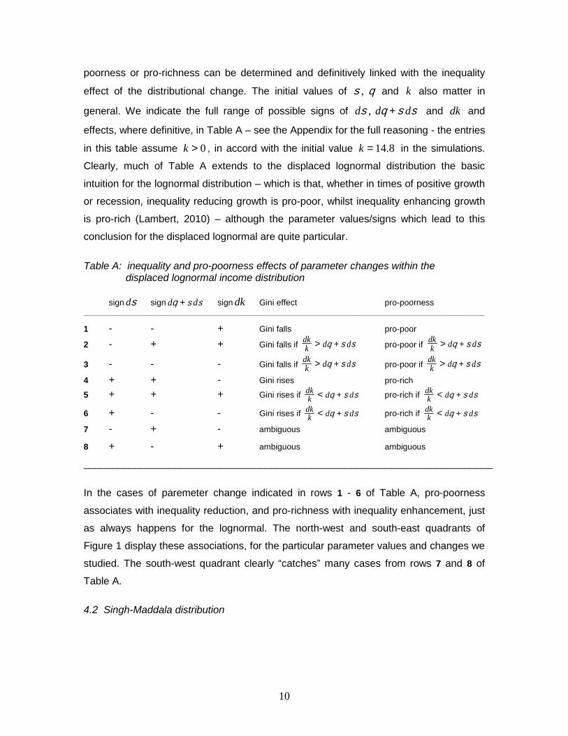
poorness or pro-richness can be determined and definitively linked with the inequality

effect of the distributional change. The initial values of s , q and k also matter in

general. We indicate the full range of possible signs of ds , dq + sds and dk and

effects, where definitive, in Table A – see the Appendix for the full reasoning - the entries

in this table assume k > 0 , in accord with the initial value k = 14.8 in the simulations.

Clearly, much of Table A extends to the displaced lognormal distribution the basic

intuition for the lognormal distribution – which is that, whether in times of positive growth

or recession, inequality reducing growth is pro-poor, whilst inequality enhancing growth

is pro-rich (Lambert, 2010) – although the parameter values/signs which lead to this

conclusion for the displaced lognormal are quite particular.

Table A: inequality and pro-poorness effects of parameter changes within the displaced lognormal income distribution sign ds sign dq + sds sign dk Gini effect pro-poorness _________________________________________________________________________________________________

1 - - + Gini falls pro-poor 2 - + + Gini falls if dk

k > dq + sds pro-poor if dkk > dq + sds

3 - - - Gini falls if dkk > dq + sds pro-poor if dk

k > dq + sds 4 + + - Gini rises pro-rich 5 + + + Gini rises if dk

k < dq + sds pro-rich if dkk < dq + sds

6 + - - Gini rises if dkk < dq + sds pro-rich if dk

k < dq + sds 7 - + - ambiguous ambiguous

8 + - + ambiguous ambiguous

________________________________________________________________________

In the cases of paremeter change indicated in rows 1 - 6 of Table A, pro-poorness

associates with inequality reduction, and pro-richness with inequality enhancement, just

as always happens for the lognormal. The north-west and south-east quadrants of

Figure 1 display these associations, for the particular parameter values and changes we

studied. The south-west quadrant clearly “catches” many cases from rows 7 and 8 of

Table A.

4.2 Singh-Maddala distribution

11

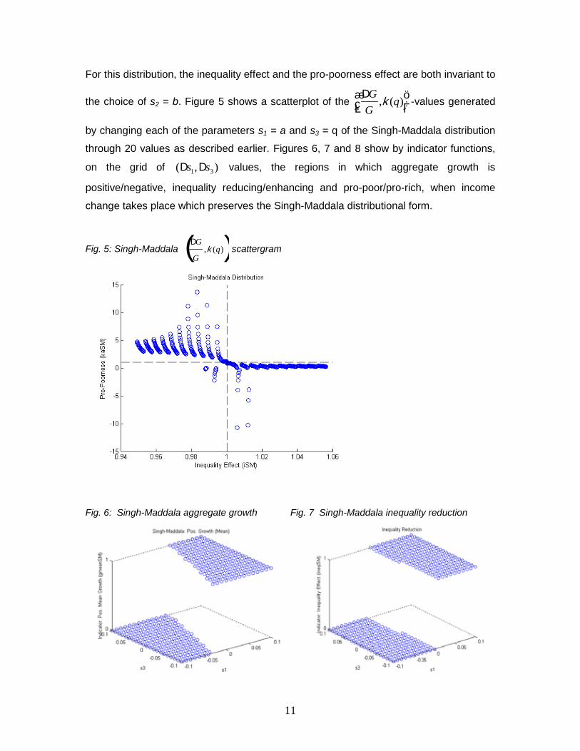
For this distribution, the inequality effect and the pro-poorness effect are both invariant to

the choice of s2 = b. Figure 5 shows a scatterplot of the DGG

,k (q)æèç

öø÷

-values generated

by changing each of the parameters s1 = a and s3 = q of the Singh-Maddala distribution

through 20 values as described earlier. Figures 6, 7 and 8 show by indicator functions,

on the grid of (Ds1,Ds3) values, the regions in which aggregate growth is

positive/negative, inequality reducing/enhancing and pro-poor/pro-rich, when income

change takes place which preserves the Singh-Maddala distributional form.

Fig. 5: Singh-Maddala DG

G,k (q)( ) scattergram

Fig. 6: Singh-Maddala aggregate growth Fig. 7 Singh-Maddala inequality reduction

12

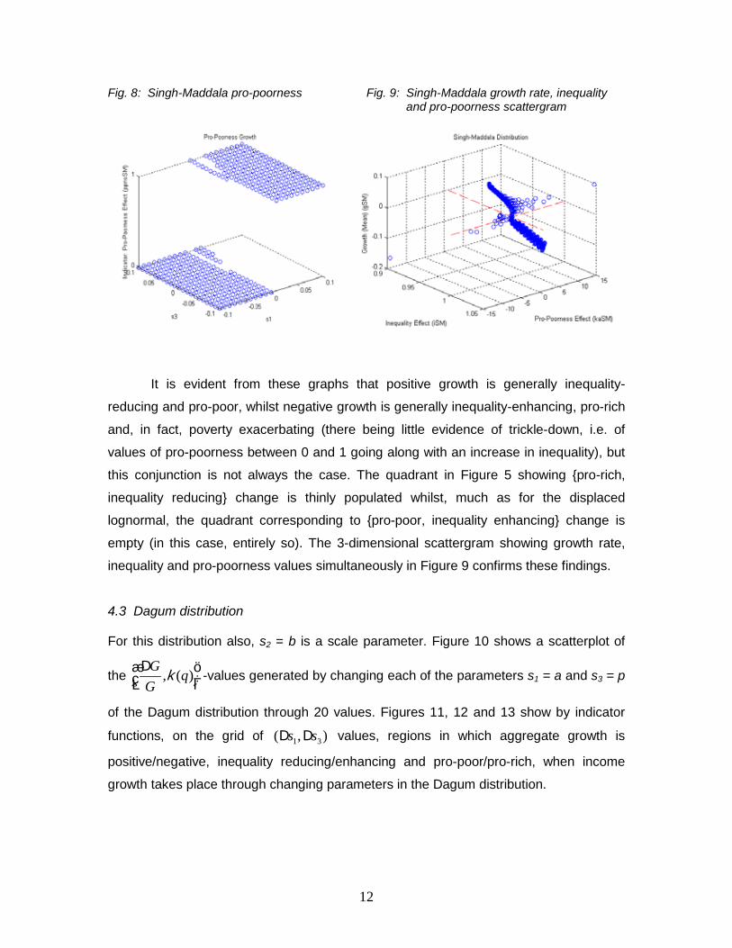
Fig. 8: Singh-Maddala pro-poorness Fig. 9: Singh-Maddala growth rate, inequality and pro-poorness scattergram

It is evident from these graphs that positive growth is generally inequality-

reducing and pro-poor, whilst negative growth is generally inequality-enhancing, pro-rich

and, in fact, poverty exacerbating (there being little evidence of trickle-down, i.e. of

values of pro-poorness between 0 and 1 going along with an increase in inequality), but

this conjunction is not always the case. The quadrant in Figure 5 showing {pro-rich,

inequality reducing} change is thinly populated whilst, much as for the displaced

lognormal, the quadrant corresponding to {pro-poor, inequality enhancing} change is

empty (in this case, entirely so). The 3-dimensional scattergram showing growth rate,

inequality and pro-poorness values simultaneously in Figure 9 confirms these findings.

4.3 Dagum distribution

For this distribution also, s2 = b is a scale parameter. Figure 10 shows a scatterplot of

the DGG

,k (q)æèç

öø÷

-values generated by changing each of the parameters s1 = a and s3 = p

of the Dagum distribution through 20 values. Figures 11, 12 and 13 show by indicator

functions, on the grid of (Ds1,Ds3) values, regions in which aggregate growth is

positive/negative, inequality reducing/enhancing and pro-poor/pro-rich, when income

growth takes place through changing parameters in the Dagum distribution.

13

Fig. 10: Dagum DG

G,k (q)( ) scattergram

Fig. 11: Dagum aggregate growth Fig. 12: Dagum inequality reduction

Fig. 13: Dagum pro-poorness Fig. 14: Dagum growth rate, inequality and pro-poorness scattergram

14

As in the Singh-Maddala case, positive growth is generally inequality-reducing

and pro-poor, whilst negative growth is generally inequality-enhancing and pro-rich.

Again, the quadrant in the scattergram (in Figure 10) showing {pro-rich, inequality

reducing} changes is thinly populated, and, as for both the displaced lognormal and

Singh-Maddala distributions, the quadrant corresponding to {pro-poor, inequality

enhancing} change is essentially empty. There is some evidence of trickle-down growth.

These findings are also very clear in the 3-dimensional scattergram showing growth rate,

inequality and pro-poorness values simultaneously in Figure 14.

5. Concluding discussion We have shown by these simulations, that for empirically relevant 3-parameter

income distributions, comprising the displaced lognormal distribution fitted to USSR per

capita income in 1990, and the Singh-Maddala and Dagum distributions fitted to United

States CPS data also for 1990, when distributional change preserves the form of the

income distribution, pro-poorness and inequality reduction ‘generally’ occur

concomitantly, as do pro-richness and inequality exacerbation, although cases do occur

in which distributional change is both pro-rich and inequality reducing. We did not,

however, find any configurations in which distributional change was both pro-poor and

inequality exacerbating using any of these distributions. The displaced lognormal was

better able to model Kakwani and Pernia’s (2000) trickle-down growth scenario than

either the Singh-Maddala or Dagum.

The poverty index we used was the familiar Watts (1969) index, and the

inequality index we used was the similarly well-known Gini coefficient. The study could

be repeated with other choices of poverty and inequality index, of course, and pro-poor

and inequality exacerbating changes might be uncovered, but it seems unlikely that the

main gist of these findings would be overturned. Just as is tautologically true of the

lognormal distribution in all cases, we have associated pro-poorness with inequality

reduction and pro-richness with inequality exacerbation in very many cases of parameter

change within the selected 3-parameter models of income distribution.

15

Appendix: analysis of displaced lognormal distribution

By assumption y = x - k is lognormally distributed with parameters s and q , so that

n(y) = q + ns where n : N(0,1) . The mean of y is u = exp{q + 12 s 2 } and the mean of x

is m = u + k . We assume k > 0 in what follows, to accord with the empirical value

k = 1.2 used in the simulations. When parameters change, let the proportional growth

rates of u and m be g = dl n u and g = dl n m respectively and let Q(y) be the

elasticity function measuring the percentage change in y per unit percentage change in

g . As shown in Lambert (2010), if q increases to q + dq and s increases to s + ds ,

then, provided g ¹ 0 , l n 1+ g Q( y)

1+ gìíî

üýþ

= ds n - s - 12

ds( ) Þ l n 1 + g Q( y)

1 + g

ìíî

üýþ

=

ds

sl n y - q - s 2 - 1

2 s ds( ). Let the poverty line be z < m (so that society is not destitute,

Cowell, 1988). For x < z we have y < z - k < u , i.e. n y < q + 1

2 s 2 , so that

l n 1 + g Q( y)

1 + g

ìíî

üýþ

¸ds

s< - 1

2 s 2 + s ds( )< 0 . Therefore, for any y < u ,

(A) g Q(y) - g <

> 0 according as ds

>

< 0 .

The means of x and y grow by respectively gm and gu dollars in the growth process,

and the dollar increase experienced by an income unit having x before growth is

gxq(x) = g yQ( y) + dk , where q(x) is the growth pattern. Thus firstly dk = gm - gu , from

which

(B) g - g =dk - kg

m ><

0 Û dkk

><

g

and secondly g xq(x) - m[ ]= g yQ(y) - u[ ], i.e. g q(x) - 1[ ]= g - g( ) m

x- 1æ

èöø +

y g Q(y) - g[ ]x

"x, y = x - k , from which, using (A), for a poor income x < z we have

(C) g q(x) - 1[ ] <

> g - g( ) m

x- 1æ

èçöø÷

according as ds >

< 0

We consider the set of parameter changes {ds ,dq + sds ,dk} rather than {ds ,dq,dk}

(for convenience since g = dq + sds ). For some sign configurations in the set

16

{ds ,dq + sds ,dk} , g - g can be signed from (B), and then g - g( ) m

x- 1æ

èçöø÷

is

unambiguously signed in (C) for all x < m . In times of either positive growth or recession,

g q(x) - 1[ ]> 0 "x < z ensures pro-poorness and g q(x) - 1[ ]< 0 "x < z ensures pro-

richness (recall the earlier discussion). The eight sign possibilities for the set

{ds ,dq + sds ,dk} of parameter changes, and implied signs of g - g where known,

are shown in Table 1 below, along with the pro-poorness or pro-richness of the

distributional change, where this can be ascertained using (C).

Table 1

sign ds sign dq + sds sign dk sign g - g pro-poorness ______________________________________________________________________________

1 - - + + pro-poor 2 - + + ? pro-poor if g > g 3 - - - ? pro-poor if g > g 4 + + - - pro-rich 5 + + + ? pro-rich if g < g 6 + - - ? pro-rich if g < g 7 - + - - ? 8 + - + + ? _________________________________________________________

The Gini coefficient of income inequality can be written as G =u

u + kæèç

öø÷

2Fs

2

æè

öø - 1é

ëêùûú

where F(×) is the N(0,1) distribution function. Evidently G is increasing in s ,

decreasing in k and, since we assume here that k > 0 , increasing in dq + sds . Thus

the Gini effect is unambiguous for the parameter configurations in rows 1 and 4 in Table

1. In rows 2, 3, 5 and 6, the sign of the Gini effect can be predicated on the sign of

g - g , since du

u + k( )=k

(v + k)2du - u dk

kéë ùû =kv

(v + k)2g - dk

kéë ùû >

< 0 Û g

>

< dk

k Û

g - g <

> 0 (using (B)). Hence if g - g < 0 and ds > 0 then dG > 0 , whilst if g - g > 0 and

ds < 0 then dG < 0 . Table 2 adds the Gini effects, where known, to the pro-poorness

properties of the various distributional changes shown in Table 1.

17

Table 2

sign ds sign dq + sds sign dk sign g - g Gini effect pro-poorness _________________________________________________________________________________________________

1 - - + + Gini falls pro-poor 2 - + + ? Gini falls if g > g pro-poor if g > g 3 - - - ? Gini falls if g > g pro-poor if g > g 4 + + - - Gini rises pro-rich 5 + + + ? Gini rises if g < g pro-rich if g < g 6 + - - ? Gini rises if g < g pro-rich if g < g 7 - + - - ? ? 8 + - + + ? ? ________________________________________________________________________

Table 2 is replicated as Table A in the main text, where g >

< g is written in terms of

parameter changes, as dkk

>

< dq + sds , using (B).

References

Alexeev, M.V. and C.G. Gaddy (1992). Income distribution in the USSR in the 1980s.

Washington DC: National Council For Soviet And East European Research.

Bourguignon, F. (2003). The growth elasticity of poverty reduction: explaining

heterogeneity across countries and time periods. Chapter 1, pp. 3-26, in Eicher,

T.S. and S. J. Turnovsky (eds.) Inequality and Growth: Theory and Policy

Implications. Cambridge MA: MIT Press.

Bourguignon, F. (2010). Non-anonymous growth incidence curves, income mobility and

social welfare dominance. Journal of Economic Inequality, forthcoming.

Bresson, F. (2009). On the estimation of growth and inequality elasticities of poverty with

grouped data. Review of Income and Wealth, vol. 55(2), pp. 266-302.

Bresson, F. (2010). A general class of inequality elasticities of poverty. Journal of

Economic Inequality, vol. 8, pp. 71-100.

Cowell, F.A. (1988). Poverty measures, inequality and decomposability. In Bös, D., M.

Rose and C. Seidl (eds.) Welfare and Efficiency in Public Economics.

Heidelberg: Springer Verlag.

18

Epaulard, A., 2003. Macroeconomic performance and poverty reduction. Working Paper

No 03/72, International Monetary Fund.

Essama-Nssah, B. and P.J. Lambert (2009). Measuring pro-poorness: a unifying

approach with new results. Review of Income and Wealth, vol. 55, pp. 752-778.

Grimm, M. (2007). Removing the anonymity axiom in assessing pro-poor growth.

Journal of Economic Inequality, vol. 5, pp. 179–197.

Jenkins, S.P. and P. Van Kerm (2006). Trends in income inequality, pro-poor income

growth, and income mobility. Oxford Economic Papers, vol. 58, pp. 531-548.

Jenkins, S.P. and P. Van Kerm (2011). Trends in individual income growth:

measurement methods and British evidence. Working Paper No. 2011-06,

Institute for Social and Economic Research, University of Essex.

Kalwij, A., Verschoor, A., 2006. Globalisation and poverty trends across regions. The

role of variation in the income and inequality elasticities of poverty. In Nissanke,

M. and E. Thorbecke (eds.), The Impact of Globalization on the World’s Poor.

Palgrave Macmillan.

Kalwij, A. and A. Verschoor (2007). Not by growth alone: the role of the distribution of

income in regional diversity in poverty reduction. European Economic Review,

vol. 51 pp. 805–829

Kakwani, N.C. and E.M. Pernia (2000). What is pro-poor growth? Asian Development

Review, vol. 18, pp. 1-16.

Klasen, S. and M. Misselhorn (2006). Determinants of the growth semi-elasticity of

poverty reduction. No. 15, Proceedings of the 2006 German Development

Economics Conference, Berlin.

Kleiber, C. (1996). Dagum vs. Singh-Maddala income distributions. Economics Letters,

vol. 53 , pp. 265-268.

Lambert, P.J. (2010). Pro-poor growth and the lognormal income distribution. Journal of

Income Distribution, vol. 19, pp. 88-99.

López, J.H. and L. Servén (2006). A normal relationship? Poverty, growth, and

inequality. Policy Research Working Paper No. 3814, World Bank.

19

McDonald, J.B. (1984). Some generalized functions for the size distribution of income.

Econometrica, vol. 52, pp. 647-663.

McDonald, J.B. and A. Mantrala (1995). The distribution of personal income: revisited.

Journal of Applied Econometrics, vol. 10, pp. 201-204.

Osmani, S. (2005). Defining pro-poor growth. One Pager Number 9, International

Poverty Center, Brasil.

Ravallion, M. and S. Chen (2003). Measuring pro-poor growth. Economics Letters, vol.

78, pp. 93-99.

Watts, H. (1968). An economic definition of poverty. Pages 316-329 in Daniel P.

Moynihan, ed., On Understanding Poverty: Perspectives from the Social

Sciences. Basic Books, New York, 1968.

Wilfling, B. and Krämer, W. (1993). The Lorenz-ordering of Singh-Maddala income

distributions, Economics Letters, vol. 43: pp. 53–57.