The Price Effects of Cash Versus In-Kind Transfers∗

Jesse M. Cunha

Naval Postgraduate School

Giacomo De Giorgi

GSEM-University of Geneva

Seema Jayachandran

Northwestern University

November 2017

Abstract

This paper examines the effect of cash versus in-kind transfers on local prices. Both types

of transfers increase the demand for normal goods; in-kind transfers also increase supply in

recipient communities, which could lead to lower prices than under cash transfers. We test and

confirm this prediction using a program in Mexico that randomly assigned villages to receive

boxes of food (trucked into the village), equivalently-valued cash transfers, or no transfers. We

find that prices are significantly lower under in-kind transfers compared to cash transfers; rel-

ative to the control group, in-kind transfers cause a 4 percent fall in prices while cash transfers

cause a positive but negligible increase in prices. In the more economically developed villages

in the sample, households’ purchasing power is only modestly affected by these price effects.

In the less developed villages, the price effects are much larger in magnitude, which we show

is due to these villages being less tied to the outside economy and having less competition

among local suppliers.

∗We thank the editor and five anonymous referees, as well as Steve Coate, Rebecca Dizon-Ross, Liran Einav,Fred Finan, Amy Finkelstein, Rema Hanna, Ilyana Kuziemko, Karthik Muralidharan, Paul Niehaus, Ben Olken,Jonathan Robinson, and several seminar and conference participants for helpful comments. Jose Marıa Nunez,Bernardo Garcia Bulle, Andres Drenik and Alexander Persaud provided excellent research assistance. Jayachan-dran acknowledges financial support from the National Science Foundation under Grant No. 1156941, and De Giorgiacknowledges financial support from the Spanish Ministry of Economy and Competitiveness, grants ECO2011-28822and the Severo Ochoa Programme for Centres of Excellence in R&D (SEV-2011-0075); and the EU through theMarie Curie CIG grant FP7-631510. Authors’ contact information: jcunha@nps.edu; giacomo.degiorgi@gmail.com;seema@northwestern.edu.

1. IntroductionA central question in anti-poverty policy is whether transfers should be made in kind or as cash.

The rationales for in-kind transfers include encouraging consumption of particular goods or induc-

ing the less needy to self-select out of the program (Besley, 1988; Nichols and Zeckhauser, 1982;

Blackorby and Donaldson, 1988; Besley and Coate, 1991; Bearse, Glomm, and Janeba, 2000).

These potential benefits of in-kind transfers are weighed against the fact that cash transfers typi-

cally have lower administrative costs and give recipients greater freedom over their consumption.

Another potentially important but less discussed aspect of this policy tradeoff is the effect

that in-kind and cash transfers have on local prices. Cash transfers increase the demand for normal

goods, which will lead to price increases. This prediction holds either with perfect competition and

marginal costs that are increasing in quantity, or with imperfect competition even if marginal costs

are constant or decreasing (under certain assumptions about demand, as we discuss in detail later).

In-kind transfers similarly increase demand through an income effect, but, in addition, if they

increase local supply (e.g., the government trucks food aid into a village), then local prices should

be lower under in-kind transfers, relative to cash transfers.1 From local suppliers’ viewpoint, an in-

kind transfer consists of a negative shock to the residual demand they face because the transfer has

met some of consumers’ demand, plus a positive demand shock due to consumers having higher

income.

The pecuniary effects could potentially be a useful policy lever, as noted by the previous litera-

ture.2 For example, the price declines caused by in-kind transfers could serve as a second-best way

to tax producers and redistribute to consumers (Coate, Johnson, and Zeckhauser, 1994). Similarly,

Coate (1989) discusses how price effects could make an in-kind food aid program more effective

than a cash program, depending on the market structure. And even if the main rationale for in-kind

transfers is paternalism or self-targeting and the pecuniary effects are an unintended consequence,

they might significantly enhance or diminish the program goal of assisting the poor.3 Note that

1Transfers can also take the form of vouchers, as in the U.S. Food Stamp and WIC programs. In this case theprogram increases demand for certain goods but local supply is not directly affected. We are considering in-kindtransfers in which the government delivers the goods or services (e.g., public housing projects in the U.S., the HeadStart program), rather than providing vouchers. In addition, the type of transfer we consider is one in which the supplyis sourced from outside the economy that receives the transfer.

2We refer to the effects we study as “price effects” or “pecuniary effects.” The data do not allow for a full exami-nation of general equilibrium effects including effects outside the market for food or outside the recipient villages.

3Another rationale for in-kind transfers is to insulate consumers from price volatility. The welfare effects ofinsurance against price fluctuations are more often discussed in the context of price stabilization policies (Massell,1969; Deaton, 1989; Newbery, 1989). Lower prices also would further boost consumption of the in-kind goods (forboth program recipients and non-recipients); if encouraging consumption of these items is the paternalistic motive forusing in-kind transfers, then the price effects will reinforce this program goal.

1

under perfect competition, the price effects shift wealth between buyers and sellers, while with im-

perfect competition and prices above the first-best level, lower prices induced by in-kind transfers

could represent an increase in efficiency, relative to cash transfers.

This paper tests for price effects of in-kind transfers versus cash transfers in rural Mexico and

compares both to the status quo of no transfers. We study a large food assistance program for poor

households, the Programa de Apoyo Alimentario (PAL). When rolling out the program, the gov-

ernment selected around 200 villages for a village-level randomized experiment. The poor in some

of the villages received monthly in-kind transfers of packaged food (rice, vegetable oil, canned

fish, etc.) that were trucked in by the government. The market value of the food transfer was about

200 pesos (20 US dollars) per household per month; most of the in-kind transfer was inframarginal

to households’ consumption.4 In other villages, the poor households received monthly cash trans-

fers of similar value to the in-kind transfer. A third set of villages served as a control group. The

vast majority of households in the villages, 89 percent on average, were eligible for the program.

A comparison of the cash-transfer villages to the control villages provides an estimate of the

price effect of cash transfers, which should be positive for normal goods since the income effect

shifts the demand curve outward. The PAL in-kind transfer has a higher nominal value than the

cash transfer (due to the idiosyncratic way that PAL administrators calculated the cost of the in-

kind bundle). The in-kind bundle’s true value to recipients is, coincidentally, very similar to the

cash transfer on average (Cunha, 2014). Therefore, the income effect in the in-kind villages should

be similar to that in the cash villages, and a comparison of in-kind and cash villages isolates the

supply effect of an in-kind transfer—the change in prices caused by the influx of goods into the

local economy. This supply effect should cause a decline in prices. We use pre- and post-program

price data collected from households and food stores to test these predictions.

We find no detectable increase in prices under cash transfers (though the point estimate suggests

a small increase), while in-kind transfers cause prices of the transferred goods to fall by 3.7 percent.

Across several specifications, we consistently find that providing transfers in kind rather than as

cash causes prices to be lower by 3 to 4 percent. These effects are not limited to the short run; over

the full range of program duration in the data, from 8 to 22 months, the effects persist. Thus, the

price effects do not appear to be undone by exit or entry of grocery shops in the village or other

changes in market structure induced by the intervention, or alternatively, such adjustments take

several years to materialize.

Goods that are not part of the transfer program are also subject to pecuniary effects. The supply

4Throughout the paper, when we calculate the nominal value of the transfer, we use pre-program unit values.

2

influx from the in-kind transfer should lower demand and prices for food items that are substitutes

of the in-kind items. Empirically, the price effects for these other goods are small. Therefore,

all told, the price effects have only modest implications for many households’ purchasing power.

This is noteworthy because program eligibility is very high and the transfer is large relative to food

expenditures, both of which result in a large aggregate shock to the local economy. This finding

of, on average, small price effects, suggests that for typical transfer programs, price effects may

not be economically significant in many communities.

The exception is the less developed villages in our sample, as proxied by low average income,

small population, and physical remoteness. In fact, the average effects we find are driven almost

entirely by the subsample of villages with below-median development.5 These villages could have

larger price effects for at least two reasons. First, their goods markets could be less integrated with

the regional or world economy, so local supply and demand determine prices. Second, there could

be less competition among local suppliers (e.g., among grocery shops or distributors supplying

those shops). We find evidence that both mechanisms help explain the result. Furthermore, surveys

of store owners in a subsample of villages point to imperfect competition as a key feature of the

market structure and an important factor in understanding the pronounced price effects in less

developed villages.

For the less developed villages, in-kind transfers cause prices of the transferred goods to fall

by 5 percent relative to cash transfers. In addition, cash transfers lead to a 1.5 percent increase in

overall food prices; this implies an elasticity of prices with respect to income of 0.15, as the cash

transfers in less developed villages constitute a 10 percent increase in aggregate income, on av-

erage. Choosing in-kind rather than cash transfers generates extra indirect transfers to consumers

in the form of lower prices worth about 14 percent of the direct transfer itself in less developed

villages; these effects have the opposite implication for food-producing households in the recipient

villages. We should note that our estimates of the program’s total effects have wide confidence

intervals, but they are nonetheless suggestive of quantitatively important price effects in poor com-

munities. Mexico’s very poor villages have a similar level of development—income level and

physical remoteness—as many villages in Africa, Asia, and Central America (World Bank, 1994).

Our results suggest that transfer programs in ultra-poor communities in developing countries may

have important pecuniary effects. Meanwhile, if the recipient community is well-connected with

larger markets or has a competitive supply side, or in general is more developed, then pecuniary

5Consistent with this finding, Angelucci and De Giorgi (2009) do not find price effects of conditional cash transfersin Oportunidades villages in Mexico, which are more developed than the PAL villages.

3

effects are likely to be small relative to the direct benefits of transfer programs.

This paper contributes to the literature on in-kind transfers, which has mostly focused on the

consumption effects of in-kind transfers and on the political economy of transfer programs. (See

Currie and Gahvari (2008) for a nice review of this literature.) Several studies have examined

the consumption effects of the PAL program in Mexico (Gonzalez-Cossio et al., 2006; Skoufias,

Unar, and Gonzalez-Cossio, 2008; Leroy et al., 2010; Cunha, 2014). They broadly find that cash

and in-kind transfers lead to similar increases in total expenditures, although of different types

of foods and non-foods. There is also extensive work on the consumption effects of other transfer

programs, such as the U.S. Food Stamp program (Moffitt, 1989; Hoynes and Schanzenbach, 2009).

Other work examines whether in-kind transfers are effective at self-targeting (Reeder, 1985; Currie

and Gruber, 1996; Jacoby, 1997). Another branch of the literature examines the political economy

of in-kind programs, including their degree of voter support and how they affect producer rents

(De Janvry, Fargeix, and Sadoulet, 1991; Jones, 1996).

Fewer studies provide evidence on the question this paper addresses, namely the price effects

of in-kind transfers, and those that do often focus on voucher programs in which the government

does not act as a supplier (Murray, 1999; Finkelstein, 2007; Hastings and Washington, 2010).6

Another related literature is on international food aid and local prices, but few of the papers in this

literature aim to establish causality; for example, Levinsohn and McMillan (2007) use estimates

of the supply and demand elasticity of food from the literature to gauge the potential price effect

of food aid, and Garg et al. (2013) examine food aid and prices, but emphasize that their estimates

are correlations and not necessarily causal effects.

Our paper is also one of the first to measure the price effects of social programs. There is a vast

literature that studies the direct effects of social programs, but fewer studies examine the indirect

effects of programs and in particular their market-level price effects (Lise, Seitz, and Smith, 2004;

Angelucci and De Giorgi, 2009; Kaboski and Townsend, 2011; Imbert and Papp, 2015; Attanasio,

Meghir, and Santiago, 2012; Muralidharan, Niehaus, and Sukhtankar, 2017). Our finding that the

pecuniary effects of social programs can be quite large in underdeveloped communities is relevant

when thinking about the impacts of many other programs in developing countries.7

Finally, our findings also contribute to an active area of policy debate. One of the largest and

6Murray (1999) examines the response by private suppliers in a market where the government does provide supply,U.S. public housing. Finkelstein (2007) finds that the Medicare program caused health care prices to rise, and Hastingsand Washington (2010) find that grocery stores in the U.S. set prices higher at the time of the month when demandfrom Food Stamp recipients is higher.

7The paper is also related to a broader literature on the determinants of prices in isolated markets in developingcountries (Jayachandran, 2006; Donaldson, 2012; Atkin and Donaldson, 2015).

4

most prominent in-kind programs worldwide, the World Food Programme, is increasingly shifting

toward cash transfers, and in many developed and developing countries there is policy debate about

providing a universal basic income (UBI) (World Food Programme, 2011). Meanwhile, other

major programs are moving away from cash toward in-kind transfers. For example, in the U.S.

much of the welfare support under the Temporary Assistance for Needy Families program is now

in the form of child care, job training, and other in-kind services (Pear, 2003). For policy makers

choosing between cash and in-kind transfers, our work highlights that their choice could have non-

trivial implications for local prices in markets with imperfect competition. Moreover, when local

suppliers’ have market power, changes in local prices are not just pecuniary externalities, but have

efficiency implications too. These lessons are relevant in developing countries where most of the

poor live in rural villages. They may also be applicable in developed countries: High-poverty

neighborhoods in the United States have high participation in transfer programs such as SNAP,

and would experience large increases in average income through a UBI program; meanwhile, they

are often characterized as having few grocery stores and high food prices (Bell and Burlin, 1993;

Talukdar, 2008).

The remainder of the paper is organized as follows. Section 2 lays out the theoretical predic-

tions. Section 3 describes Mexico’s PAL program, other aspects of the context, and the experimen-

tal design. Section 4 describes our empirical strategy and data. Section 5 presents the results, and

Section 6 offers concluding remarks.

2. Conceptual FrameworkIn this section, we lay out the predictions about how cash and in-kind transfers affect prices.

We do not present a formal model but instead informally derive the predictions that we take to the

data.

In a small open economy, changes in the local demand or supply should have no effect on

prices since supply is infinitely elastic with prices set at the world level. However, the rural villages

that are our focus are more typically partially-closed economies in which prices depend on local

conditions. In our empirical application, an economy is a Mexican village, and the main goods we

examine are packaged foods. The local suppliers are shopkeepers in the village, and they procure

their inventory from outside the village.8

8There is also a supply side of the market that is outside the local economy, namely the packaged food manufac-turers, which are located in urban areas. If by increasing the total demand for the goods from food manufacturers,the government is driving up manufacturers’ marginal cost (because they have decreasing returns to scale), then therewould also be Mexico-wide price effects of the program. These effect on prices would be very small since the program

5

We discuss, in turn, two possibilities: that the supply side has perfect or imperfect competition.

In our empirical setting, imperfect competition appears to be the more relevant scenario.

Perfect competition

If the local market is perfectly competitive, then if the supply curve is positively sloped—that

is, with increasing marginal costs—shifts in the demand for a good will affect its price. For local

suppliers in Mexican villages, high transportation costs to other markets is one potential reason

for increasing marginal costs, at least in the short run; to meet higher demand, a shopkeeper in a

remote village might need to travel to a neighboring village to buy supply from a shop there.

Panel A of Figure 1 depicts the market for a normal good in a village. The demand curve

represents the aggregate demand faced by local suppliers. The figure shows, first, the effect of a

cash transfer: The demand curve shifts to the right via an income effect, and the equilibrium price,

p, increases.9 Denoting the amount of money transferred in cash by XCash, our first prediction is

that a cash transfer will cause prices to rise:

∂ p∂XCash

> 0 (1)

In-kind transfers also generate an income effect, so demand will again shift to the right. We

define the in-kind transfer amount XInKind in terms of its equivalent cash value.10 Thus the demand

shift caused by a transfer amount X is by definition the same for either form of transfer. With an

in-kind transfer, however, some of consumers’ demand is now provided to them for free by the

government, so the residual demand facing local suppliers shifts to the left by the amount provided

in kind. While the net price effect of an in-kind transfer relative to the original market equilibrium

is, in general, theoretically ambiguous, one can sign the price effect of in-kind transfers relative to

households represent less than 1 percent of Mexican households, but these small effects would apply to the large set ofconsumers of the goods. Our focus is the price effects within the villages that receive the program; thus, we examineonly the local price effects in the recipient villages, and not the total price effect of the program.

9For inferior goods, demand will shift to the left with the opposite price effect. In unreported results estimatinga QUAIDS demand function, we find that all of the food items we study are normal goods except for one (chayote).Similarly, Attanasio, Di Maro, Lechene, and Phillips (2013) find that most food items are normal goods in Mexico.

10If either the transfer is inframarginal (that is, it is less than the household would have consumed had it receivedthe transfer in cash, valued at the market prices) or resale is costless, the cash value of the transferred goods is simplythe market value. If, instead, the transfer is “extramarginal” and resale is costly, then the extramarginal quantity wouldbe valued at between the market price and the resale price.

6

cash transfers.11 For transferred goods, the price should be lower under in-kind transfers:

∂ p∂XInKind

− ∂ p∂XCash

< 0. (2)

Empirically, we will be better positioned to test Prediction (2) than Prediction (1). To detect

the effect of the supply influx, we can concentrate on the nine specific goods provided in kind in

the Mexican transfer program we study. In contrast, the increased demand due to income effects

will be spread across several food and non-food items. The cash transfer program we study placed

no restriction on how recipients could use the money, and it led to a small amount of extra demand

per good, spread across many goods (Cunha, 2014).12,13

Imperfect competition

In the setting we study, the supply side consists of food shops in the village and the distributors

who supply the shops, trucking in food from outside the village. There are neither many shops nor

distributors serving the typical village, so the degree of competition may be limited.

Predictions (1) and (2) can also hold in the case of imperfect competition. Importantly, in

contrast to the case of competitive firms, under imperfect competition, transfer programs can have

price effects even if marginal costs are constant. Panel B of Figure 1 depicts, for simplicity, the

case of constant marginal cost for a monopolist facing linear demand, but the same predictions of

price effects hold more generally, as we discuss below.

Consider a Cournot-Nash model with N firms that have constant marginal cost c and face linear

demand p = d−Q, where Q indicates quantity and d represents factors that shift demand. The

equilibrium price is p = (d +Nc)/(N + 1). Suppose the transfer changes the amount demanded

from the local firms by an amount ∆d; ∆d is positive for a cash transfer and negative or less positive

for an in-kind transfer. Then the change in price is given by ∆p/p = ∆d/(d +Nc), which has the

property that the higher N is (more competition), the smaller the magnitude of the price effects.

More generally, the price effects under imperfect competition depend on the shape of the de-

mand curve. For example, if the program causes a multiplicative shift in demand, then there would

be no effect on prices in the standard Cournot model (Cowan, 2004). In other cases, an increase

11For many standard classes of preferences, such as homothetic preferences, prices are predicted to decline with anin-kind transfer relative to no transfer. For the price to increase, an in-kind transfer of a good with aggregate value Xwould need to increase aggregate demand for the good by more than X ; in other words, the good would have to be astrong luxury good.

12Cunha (2014) shows that 17% of the cash transfer is spent on PAL foods, while 50% is spent on non-PAL foodsand 33% is spent on non-food goods.

13Note that there could be a flypaper effect through which this cash transfer labeled as food assistance stimulatedthe demand for food more than a generically-labeled transfer would have (Hines and Thaler, 1995; Kooreman, 2000).

7

in demand can cause oligopolistic prices to fall; greater competition would still dampen the mag-

nitude of the price effects. Appendix A presents a Cournot model with a generalized demand

function and shows conditions under which an increase in demand leads to a higher price. A suf-

ficient condition for Predictions 1 and 2 to hold is a downward-sloping demand curve where the

transfers represent an additive shift in demand. The price effects then vary with the degree of

competition as follows:∂ 2 p

∂N∂XCash< 0, (3)

and∂

∂N

(∂ p

∂XInKind− ∂ p

∂XCash

)> 0. (4)

The higher N is (more competition), the smaller in magnitude the price effect of a demand shift.

Note that price effects under perfect and imperfect competition have different efficiency impli-

cations. If lack of competition causes prices to be above their efficient level, then in-kind transfers

can increase total surplus. Local suppliers’ strategic rationing of supply is partly undone by the

government provision of goods. (Note, however, that these potential welfare gains could be undone

by inefficiencies in how the government runs the transfer program.)

The discussion above takes the market structure as given. The program could also affect how

many stores stock a given product as well as entry and exit of stores and thus the degree of com-

petition. For example, in response to a supply influx from the government, a shop might stop

carrying a product or go out of business, reducing competition and causing prices to return to, or

even exceed, the counterfactual price level without the program. A positive demand shock (e.g.,

due to a cash transfer) could cause stores to open or more stores to stock a given good, increasing

competition. The theoretical predictions are not clear-cut in many cases. For example, the in-kind

program also made villagers richer, so the net effect on store entry and exit or inventory decisions is

ambiguous. In addition, the price effect of a store beginning to or ceasing to stock a product is not

easy to predict because firms do not profit maximize separately for each product. Nonetheless, in

general these responses on the supply side would cause price effects to be smaller. These changes

would likely not occur immediately, but as they occur, the price effects would fade. Thus, we also

examine whether the price effects dissipate over time.

The above are the main testable implications we take to the data. We next describe the transfer

program we study and discuss some of the above assumptions in the context of this program.

8

3. Description of the PAL Program and Context

3.1 PAL program and experiment

We study the Programa de Apoyo Alimentario (PAL) in Mexico. Started in late 2003, PAL

operates in about 5,000 very poor, rural villages throughout Mexico. Villages are eligible to receive

PAL if they have fewer than 2,500 inhabitants, are highly marginalized as classified by the Census

Bureau, and do not receive aid from either Liconsa, the Mexican subsidized milk program, or

Oportunidades, the conditional cash transfer program. Therefore PAL villages are typically poorer

and more rural than the widely-studied Progresa/Oportunidades villages.14 Households within

program villages are eligible to receive transfers if they are classified as poor by the national

government.

PAL provides a monthly in-kind allotment consisting of seven basic items (corn flour, rice,

beans, pasta, biscuits (cookies), fortified powdered milk, and vegetable oil) and two to four supple-

mentary items (including canned tuna fish, canned sardines, lentils, corn starch, chocolate powder,

and packaged breakfast cereal). All of the items are common Mexican brands and are typically

available in local food shops. The basic goods are dietary staples for poor households in Mexico.

The supplementary goods are foods typically consumed by fewer households in a village or less

frequently; one goal of the program was to encourage households to add diversity to their diet and

consume more of these supplementary goods.15

Most recipient households consumed a larger quantity of the in-kind items, particularly the

basic goods, than was provided in the transfer. That is, absent the transfer, their monthly quantity

consumed exceeded the PAL in-kind allotment. The fact that recipients made out-of-pocket pur-

chases of these goods even when receiving the in-kind transfer means that they were affected by the

price effects; otherwise, price effects would only be relevant for non-recipients. Figure 2 shows the

net-of-transfer expenditures on PAL goods (calculated using post-intervention expenditure in the

control group).16 The poorest quartile of households spends slightly more than the richest quartile

14Villages could be “too poor” to receive Progresa/Oportunidades because a requirement was that they had thecapacity to meet the extra demand for prenatal visits and school attendance induced by the program; villages thatlacked adequate health facilities, for example, were ineligible for Progresa/Oportunidades.

15Appendix Figures 1 to 4 show the PAL box, trucks transporting the boxes to a village, the unloading of the boxesin the village, and examples of the grocery shops in the villages.

16We use the good-by-good quantity consumed and subtract the quantity of the PAL allotment for that good, andthen multiply by the price. If the aggregate transfer to a village exceeds the village’s aggregate consumption of agood, we set out-of-pocket spending for the village-good to zero; this allows for within-village resale but assumesthere is no resale outside the village. For two food items (powdered milk and lentils), villages consumed less than theamount delivered in kind, while for the other goods (e.g., vegetable oil, beans), they consumed more per month thanthe transfer.

9

on these items, and spends more as a proportion of total food expenditures. Most of the PAL items

are staple goods, which explains why they comprise a larger share of food spending for the poor.

PAL is administered by the public/private agency, Diconsa. The Diconsa agency also maintains

subsidized grocery shops in some villages (38 percent of the villages in our sample), which are run

by a resident of the village. The government provides suggested prices to Diconsa store operators;

the Diconsa stores are not obliged to use the suggested prices, but they must maintain prices that

are three to seven percent lower than market prices. Thus, prices at Diconsa stores should be

responsive to market conditions, but to a lesser degree than at fully private stores.17 The local

supply side of the market is mostly comprised of small private stores that stock food products,

including the packaged foods that PAL provided, as well as sundry items. Small villages typically

have one to six of these types of stores. Some households in the village also grow food which is

substitutable with the PAL packaged foods.

Concurrent with the national roll-out of the program, 208 villages in southern Mexico were

randomly selected for inclusion in an experiment.18 Each study village was then randomly as-

signed to an in-kind treatment arm, cash treatment arm, or the control group; the village-level

randomization was not stratified on any characteristics. Eligible households in the in-kind villages

received a monthly in-kind food transfer (50 percent of villages); those in the cash villages received

a 150 peso per month cash transfer (25 percent of villages); and those in the control group villages

received nothing (the remaining 25 percent of villages). About 89 percent of households in the

in-kind and cash villages were eligible to receive transfers (and received them). Due to adminis-

trative capacity constraints, experimental villages were rolled into the program over the course of

14 months, beginning in December of 2003. This gradual rollout creates variation in how long the

program had been running when endline data collection occurred in 2005.

Of the 208 villages in the experiment, 14 are excluded from the analysis. Eight villages do

not have follow-up price data; in two villages, the PAL program began before the baseline survey;

two villages are geographically contiguous and cannot be regarded as separate villages; and two

villages were deemed ineligible for the experiment because they were receiving the conditional

cash program, Oportunidades, contrary to PAL regulations.19 Observable characteristics of the

17Diconsa stores receive a government subsidy to cover transportation costs. Unlike fully private shops, they donot allow purchases on credit. After our study period, the government changed the discount that Diconsa stores aresupposed to offer to 20 percent (private communication with program administrators).

18The experiment was implemented in eight states: Campeche, Chiapas, Guerrero, Oaxaca, Quintana Roo, Tabasco,Veracruz, and Yucatan. The 208 study villages were randomly chosen from among all PAL-eligible villages in thesestates, without stratification. See Appendix Figure 5 for the locations of the experimental villages.

19The contiguous villages are named “Section 3 of Adalberto Tejada” and “Section 4 of Adalberto Tejada,” whichappear to be part of the same administrative unit. The correlation of baseline unit values between these two villages

10

excluded villages are balanced across treatment arms. (Results available from the authors.) Of

the remaining 194 villages, three received the wrong treatment (one in-kind village did not receive

the program, one cash village received both in-kind and cash transfers, and one control village

received in-kind transfers). We include these villages and interpret our estimates as intent-to-treat

estimates.

The aggregate impact of the PAL program on a recipient village was large, both because the

eligibility rate was high and because the transfer per household was sizeable. The in-kind transfer

represented 18 percent of a recipient household’s baseline food expenditures on average and 11

percent of total expenditures. Including the ineligible households, the injection of food into the

village through the program was equivalent to 16 percent of baseline aggregate food expenditures

and 10 percent of total expenditures for the village. Similarly, the cash transfer represented an

8 percent increase in recipients’ income and, in aggregate, a 7 percent increase in total village

income.

In the in-kind experimental villages, the transfer comprised the seven basic items and three sup-

plementary goods: lentils, breakfast cereal, and either canned tuna fish or canned sardines. There

is some ambiguity about whether the in-kind villages always received these three supplementary

items, so, in our some of our analyses, we separate the basic PAL goods from the supplementary

ones. Another reason to examine the basic goods separately is that they isolate the simple income

and supply effects of in-kind transfers; if the government succeeded in increasing households’

taste for the supplementary goods, then the supplementary goods would have an additional effect

of changing preferences (which goes in the direction of increasing demand and prices). The market

for basic goods is also thicker, so the price effects might be easier to detect for the basic goods.

Both the in-kind and cash transfers were, in practice, delivered bimonthly, two monthly al-

lotments at a time per household. A woman (the household head or spouse of the head) was

designated the beneficiary within the household, if possible. The transfer size was the same for

every eligible household regardless of family size. Resale of in-kind food transfers was not pro-

hibited, nor were there purchase requirements attached to the cash transfers. The monthly box of

food had a market value of about 206 pesos in the program villages, and the cash transfer was 150

pesos per month, based on the government’s wholesale cost of procuring the in-kind items.20 The

is 0.92. When we take random draws of pairs of villages in our sample and calculate the correlation of baseline unitvalues, the 99th percentile is a correlation of 0.51, suggesting that the contiguous pair is an extreme outlier and cannotbe treated as two distinct markets. Our results are robust to including them in the analysis, however.

20The government should have included its transportation costs when calculating the in-kind program’s costs. Thisoversight attenuates the in-kind-versus-cash price differential that is our main focus; a 206 peso cash transfer wouldhave led to a larger price increase in cash villages, so a larger relative price decline in in-kind villages.

11

items included in the in-kind transfer are not produced locally.21 Thus, the main welfare effects

on the local supply side of the market will be felt by shopkeepers. There will also be welfare

effects for local agricultural producers in cases where there is a high degree of substitutability (or

complementarity) between the in-kind goods and the local products.

An inconvenient feature of the program for our purposes is that the cash villages and a randomly

selected half of the in-kind villages were assigned to receive health, hygiene, and nutrition classes,

as well. This program feature could create two potential problems for the interpretation of our

results. First, the difference between the price effects of cash and in-kind transfers, which we

interpret as due to the injection of supply, could be partly driven by differential exposure to the

classes. Second, the impact of cash transfers on prices could be partly driven by the classes, rather

than being a pure income effect.

These concerns appear to be small in practice. Regarding the first concern (in-kind versus cash),

as documented in the appendix, when we restrict the sample to in-kind villages assigned to receive

classes—that is, if we analyze in-kind and cash villages that do not differ in their assignment to

classes—the cash-versus-in-kind price effect is very similar to our main results that use all of the

in-kind villages. This finding is not surprising given that classes were actually offered in almost all

of the in-kind villages assigned not to receive them (Cunha, 2014).22 Thus, in practice, the cash and

in-kind treatment arms were essentially identical vis-a-vis classes, and it seems valid to interpret

the in-kind versus cash comparison as due to the supply effect. For the second concern (cash versus

control), there is no experimental variation to exploit, but when we compare class attendees to non-

attendees in the cash arm, there is no evidence that the classes shifted food consumption, either

overall or toward the PAL foods (as shown in the appendix). This evidence makes us doubtful

that the classes affected prices in the cash treatment arm, though attendance is endogenous so this

evidence is only suggestive. Therefore, the caveat that the classes may have played some role in

the price effect of cash transfers should be kept in mind when interpreting our cash versus control

effect as a pure income effect. We abstract from this component of the program for the remainder

of our analysis.

21We do not observe actual food production, but rather draw this conclusion from household survey data on con-sumption of own-produced foods. The only PAL good that has auto-consumption in any appreciable quantity is beans(10 percent of households consume own-produced beans at baseline). There is also relatively little auto-consumptionof non-PAL foods. Only 7 out of 60 foods in our analysis have more than 10 percent of the population producing thegood, the largest of which is corn kernels, which 27 percent of households produce.

22Based on the household survey data, 76 percent of respondents attended a class in the in-kind villages assignedto receive classes and 69 percent attended a class in the in-kind villages assigned to not receive classes. In both cases,average attendance was roughly four classes over the course of the program. Furthermore, assignment to classes didnot affect total food expenditure or the composition of food expenditure (results available from the authors).

12

3.2 Assumption of identical income effects for cash and in-kind transfers

In section 2, we expressed the size of the in-kind transfer XInKind in terms of its cash equivalent

to recipients. If one compares a cash transfer program and an in-kind transfer program, and the cash

equivalent of the in-kind transfer is exactly the same amount as the cash transfer, then the income

effect for both transfer programs is the same. Coincidentally, this is quite close to being the case

in our empirical setting. The market value of the in-kind transfer in the recipient villages averaged

206 pesos (based on pre-program prices). The in-kind bundle would have had a cash-equivalent

value of 206 pesos if the transfer was inframarginal to consumption or resale was costless, that is,

if the in-kind nature of the transfers did not distort recipients’ consumption choices. However, the

transfers did alter consumption patterns, so the cash equivalent was less than the nominal value of

206 pesos. We estimate that recipients valued it at 146 pesos on average, or 71 cents on the dollar,

as detailed in the next paragraph. The Mexican government made the (peculiar) decision to set

the cash transfer in its randomized experiment equal to its wholesale cost of procuring the in-kind

goods, which was about 27 percent lower than the cost at consumer prices in the recipient villages.

The government also did not adjust for the fact that its estimated distribution cost was 30 pesos per

in-kind box but 20 pesos per recipient for the cash transfer. The cash transfer was set at 150 pesos

per month.

There are three conceptually distinct ways that recipients use goods provided to them in kind.

First, they consume some amount of it that they would have consumed anyway; they value this

inframarginal portion at market prices. By comparing the control group’s consumption to transfer

recipients’ consumption, Cunha (2014) estimates that 116 pesos worth of the 206-peso bundle

falls in this category. Second, recipients consume an additional amount of the transferred foods,

more than they would have consumed absent the in-kind transfer. PAL recipients consumed an

estimated 35 pesos more of food in the transferred categories as a result of the in-kind transfer.

Third, recipients received an additional 55 pesos worth of goods that they did not consume and

presumably resold instead.23 For the latter two categories—the “extramarginal” portion—there is

deadweight loss, and recipients will value the goods at less than their market value. For the extra

goods they consume, they would not have been willing to purchase them at market prices, and for

the goods they resell, they likely incur transaction costs. We assume, first, that consumers value

the extramarginal consumption at a two-thirds discount relative to its market value, and second,

that for goods that are resold, transaction costs erode two thirds of their value. Thus, the 90

23Households might also store the goods, but since the program is expected to continue indefinitely, perpetualstorage and an accumulating amount of stored goods seems unlikely. In any case, there would also be some deadweightloss from storage.

13

pesos of extramarginal transfers are valued at only 30 pesos. Under these assumptions, the PAL

in-kind transfer is worth 146 pesos to recipients (116 for the inframarginal portion + 30 for the

extramarginal portion).

To recap, while it is impossible to pinpoint the precise value of the in-kind transfer to recipients—

its nominal value minus the deadweight loss relative to an unconstrained transfer—the value of the

PAL in-kind transfer was likely quite similar to the value of the cash transfer to which we compare

it (146 pesos versus 150 pesos).24 Moreover, even if consumers place zero value on the extra-

marginal portion of the in-kind transfer, valuing only the 116 pesos of inframarginal consumption,

this difference in the income effect is much too small to explain the magnitude of the cash-versus-

in-kind price effects that we estimate in Section 5, as we show in that section.

It is also worth noting that flypaper effects could be especially strong when transfers are made

in-kind: By giving households particular goods, the government might signal the high quality of

these goods (e.g., their nutritional value) and also make these items more salient to households.

In other words, with an in-kind transfer relative to a cash transfer, not just the supply but also

the demand for the transferred goods might increase. This extra effect of in-kind transfers would

counteract the supply effect, and our estimated price effects would give a lower bound for the pure

supply-shift effect of in-kind transfers.25

3.3 Market structure

As the data collected by the Mexican government for the PAL experiment did not include infor-

mation on market structure, we conducted surveys of store owners in a subsample of 52 villages to

qualitatively understand the market structure, stores’ cost curves, and their price-setting behavior.

(See Appendix B for further details on the data collection.) Several facts are worth highlighting.

First, there are few food stores per village. The median number of stores in 2015 was 4, and while

respondents could not reliably recall the number of stores at the time the PAL experiment began in

2003, they reported that the number of stores was lower at that time. Second, there are fewer stores

in less economically developed villages. Third, marginal cost curves appear to be upward-sloping

over the short run (e.g., 1 month), but flat over a longer duration. Store owners report that they

meet unexpectedly high demand by traveling to a neighboring village or town to buy goods, which

is costly, but for a permanent demand shock, they readjust the amount they procure from their24Another empirical fact that suggests that the income effects are the same for cash and in-kind villages is that we

do not observe differential impacts on two categories of goods that are plausibly separable from the PAL food items,namely food expenditure away from home and non-food expenditure. This analysis is presented in Appendix Table 1.

25A shift in preferences could also have been generated by the hygiene, health, and nutrition classes. However, asmentioned, we find no evidence of class attendance having an effect on overall food consumption or consumption ofthe PAL food items.

14

distributors on a regular basis. Finally, store owners report that they adjust their prices quickly in

response to increases or decreases in demand, usually within a week.

We interpret these facts as pointing to stores having market power and facing a flat marginal

cost curve over the one- to two-year time horizon for which we test for price effects.

4. Empirical Strategy and Data

4.1 Empirical strategy

Our analysis treats each village as a local economy and examines food prices as the outcome,

using variation across villages in whether a village was randomly assigned to in-kind transfers, cash

transfers, or no transfers. We begin by focusing on the food items included in the in-kind program.

Our first prediction is that prices will be higher in cash villages relative to control villages since a

positive income shock shifts the demand curve out (under the assumption that the items are normal

goods). The second prediction is that relative to cash villages, prices will be lower in in-kind

villages because of the supply influx.

Our main data consists of prices collected in experimental villages both pre- and post-program.

We estimate the following regression where the outcome variable is pgsv, the price for good g at

store s in village v:

pgsv = α +β1InKindv +β2Cashv +φ pgv,t−1 +σ Igv + εgsv (5)

Our two predictions correspond to β2 > 0 (cash transfers increase prices), and β1 < β2 (prices are

lower under in-kind transfers than cash transfers). In our main specification, we control for the

baseline price, denoted pgv,t−1, which does not vary within a village (see below). (The subscript

t−1 is shorthand for the variable being constructed from the baseline data; the estimation sample

is cross-sectional, not a panel over time.) We also include the dummy variable I to indicate whether

the pre-program price is imputed (again, see below). We cluster standard errors at the village level,

the level at which the treatment was randomized.

Note that a difference between the two predictions is that the first one—a positive price effect

of cash transfers—applies to all normal goods, whereas the second one—a negative price effect of

in-kind relative to cash transfers—applies to the goods provided in kind. We therefore have a more

focused (and possibly higher-powered) way to test the second prediction, namely by examining

the prices of PAL goods rather than all goods.

15

4.2 Data

The data for our analysis come from surveys of stores and households conducted in the ex-

perimental villages by trained enumerators from the Mexican National Institute of Public Health

both before and after the program was introduced. Baseline data were collected in the final quarter

of 2003 and the first quarter of 2004, before villagers knew they would be receiving the program.

Follow-up data were collected two years later in the final quarter of 2005, one to two years after

PAL transfers began in these villages. The Mexican government’s purpose in running the exper-

iment was to measure the program’s impacts on food consumption, and what type of data they

collected was determined accordingly.

Our measure of post-program prices comes from a survey of local food stores. From each store,

enumerators collected prices for fixed quantities of 66 individual food items. They were instructed

to first identify all the food stores in the village and then survey a maximum of three stores per

village; unfortunately, no data were recorded from the step where they identified all of the stores. If

more than three stores existed per village, they were instructed to randomly select three to survey,

if possible one from each of three store types: general stores with posted prices, general stores

without posted prices (e.g., small corner shops, butcher shop, or bakery), and the village market,

taken as a unit. For 37 percent of villages in our sample, one store was surveyed; for 47 percent

of villages, two stores were surveyed; and three stores were surveyed in the remaining 16 percent

of villages.26 Some of the stores surveyed were part of the Diconsa agency (21 percent) while the

majority were independent stores (79 percent).

We also use measures of pre-program food prices. Baseline data collection on store prices

are missing for 40 percent of the sample because, first, data were collected for only 40 of the 66

food items, and, second, even among the sampled goods, there are missing data for 19 percent

of village-good observations (see Appendix B for details). Therefore, we also use the household

survey to construct the pre-program unit value (expenditure divided by quantity purchased) for

each food item. In each village, a random sample of 33 households was interviewed about purchase

quantities and expenditures on 60 food items. We use the median unit value among households

in the village as a measure of the village’s pre-program price.27 In cases where the pre-program

26Many of the shops had posted prices. If prices were not posted, the enumerators were instructed to choose thelowest price available for a given good in order to maintain consistency.

27Unit values are observed for households that purchased the good in the past seven days. We do not use unit valuesfor post-program prices because the program changes the number and composition of households that purchase items.(Results available from the authors.) If the quality of a good does not vary and there is no price discrimination (e.g.,bulk discounts), then unit values could still be used as a proxy for post-program prices. However, if quality varies, thentreatment effects estimated with post-program unit values would reflect changes in both price and quality, and if thereis price discrimination across households, then the treatment effects would also reflect changes in the composition of

16

village median unit value is missing, we impute it using the median unit value in other villages

within the same municipality (or within the same state in the few cases where there are no data

for other villages in the municipality). Despite the missing data, we also use pre-program store

prices in some specifications to check the robustness of our results. The data do not allow us to

match stores between waves; therefore, we use the median store price within a village and good

as a measure of the pre-program price. When the village median store price is missing, we impute

the price using, first, the village median unit value, and then the geographic imputation of village

median unit values (as above).

To facilitate comparisons across goods with different price levels, we normalize the price for

each good by the sample mean for the good within the control group, by survey wave. (If one good

is ten times the price of another good, we would not expect the program to have the same effect

in levels for these two goods, but we would expect it to have the same proportional effect, all else

equal.) The mean price for each good is thus roughly 1, and exactly 1 for the control group. The

empirical results are nearly identical if we normalize by the mean value across all the villages, but

using the control villages seems preferable so that the normalization factor is not affected by the

treatments. We also show the results using the logarithm of the price as the outcome.

We exclude some food items from the analysis due to missing data. Among the PAL goods, the

store price survey mistakenly did not include biscuits; for the non-PAL items, chocolate powder,

nixtamalized corn flour, salt, and non-fortified powdered milk were not included in the household

survey and corn starch was not included in the store survey.28 Finally, two pairs of goods were

asked about jointly in the household survey (beef/pork and canned fish) but separately in the store

survey (beef, pork, canned tuna, canned sardines). To address this discrepancy, we use the ag-

gregated categories and take the median across all observed store prices for either good as our

post-program price measure. Our final data set comprises six basic PAL goods (corn flour, rice,

beans, pasta, oil, fortified milk), three supplementary PAL goods (canned fish, packaged breakfast

cereal, and lentils), and 51 non-PAL goods. Appendix Table 2 lists all of the goods in our analysis.

Table 1 presents descriptive statistics for the PAL goods. Column 2 shows the quantity per

good of the monthly household transfer, and column 3 shows its monetary value measured using

households purchasing a good. While quality is quite homogenous for manufactured items where there are few brandssold, it is heterogeneous for other goods (e.g., fresh food). See also McKelvey (2011) on the effect of income andprice changes on the interpretation of unit values. Also note that for some goods, there are very few household-levelobservations of the baseline unit value (e.g., lentils, cereal, corn flour), while for others, most households purchasedthe good (e.g., beans, corn kernels, onions). The noisiness of our pre-period price measure will vary with the numberof observed unit values.

28The price of biscuits was intended to be collected, but a mistake in the survey questionnaire led enumerators tocollect prices for crackers (“galletas saladas” in Spanish) rather than for biscuits (“galletas” in Spanish).

17

our pre-program measure of prices. Column 4 presents each good’s share of the total calories in

the transfer bundle. As can be seen, the supplementary items were transferred in smaller amounts

with lower value and fewer calories than the basic goods.

There is considerable variation across the PAL goods in the size of the aggregate village-level

transfer. One measure of the size of this supply shift is listed in column 5. Here, the village change

in supply, ∆Supply, is constructed as the average across in-kind villages of the total amount of

a good transferred to the village (i.e., average number of eligible households per village times

allotment per household) divided by the average consumption of the good in control villages in

the post-program period. For example, there was almost exactly as much corn flour delivered to

the villages each month as would have been consumed absent the program (∆Supply = 1.00 for

corn flour), while the allotment of beans was 29% of what would have been consumed absent the

program (∆Supply = 0.29 for beans).

Our final data set contains 360 stores in 194 villages and 12,940 good-village-store observa-

tions. The number of goods varies by store since many stores sell only a subset of goods. Table 2

presents summary statistics by treatment group. The baseline characteristics are for the most part

balanced across groups. For three variables, there are significant differences across groups at the

five percent level: The presence of a Diconsa store differs between control and in-kind, the share

of food-producing households differs between control and cash and between in-kind and cash,

and farm costs differ between control and in-kind and between control and cash. For our primary

comparison—between the cash and in-kind treatments—no variable is unbalanced at baseline at

the 5 percent level and only one variable is unbalanced at the 10 percent level.29

In some of our auxiliary analyses, we use household-level data to either construct village-

level variables or to estimate household-level regressions. For example, we calculate the median

household expenditures per capita in a village at baseline as a measure of the income level in

the village. Also, when we test for heterogeneous welfare effects for households that produce

agricultural goods, we use household-level outcomes such as farm profits and expenditures per

capita. We present more detail on other relevant data as we introduce each analysis in the next

section.

Note that the data collection was designed to measure the PAL program’s impact on food

consumption, not its price effects. It is fortunate that the price data from stores were collected,

enabling our analysis of the program’s price effects. However, other data that ideally we would

29Appendix Table 3 presents additional summary statistics of demographic and consumption variables by treatmentgroup, which further demonstrate balance.

18

have are unavailable, e.g., a census of grocery shops in each village. Thus, we do not have data

on market structure to include in the empirical analysis. (Our survey of store owners in a subset

of the villages, described in section 3.3, provides a qualitative understanding of the typical market

structure in the study villages.)

5. Results

5.1 Price effects of in-kind transfers and cash transfers

Table 3, column 1, presents the main specification (Equation 5) using all nine PAL goods. The

regression pools the effects for the different PAL food items. (See Appendix Table 4 for the results

separately for each PAL good.) For cash villages, the point estimate suggests that the transfer

program caused prices to increase by 0.2 percent (β2), though the coefficient is not statistically

significant. In in-kind villages, prices fell by 3.9 percent relative to the cash villages (β1− β2),

with a p-value of 0.02; the bottom of the table reports the difference between the in-kind and

cash coefficients and the statistical significance of this difference. As mentioned above, theory is

ambiguous about whether the supply or demand effect is bigger in magnitude, but unless a good has

a particularly high income elasticity of demand, we would expect the supply effect to dominate.

Empirically we indeed find that the net effect of the in-kind transfer on prices is negative (3.7

percent decline, significant at the 10 percent level).

The in-kind-versus-cash difference is much too large to be due to just the income effect differ-

ing between the two types of transfer programs. As discussed in Section 2, recipients valued the

in-kind bundle at roughly 146 pesos which is similar to the cash transfer amount of 150 pesos. The

coefficient on Cash of 0.002 is the effect of a 150 peso income transfer, suggesting that the 4 peso

difference would generate an in-kind-versus-cash difference in the income effect on the order of

-0.00005. Even if recipients only valued the in-kind goods that were purely inframarginal to their

consumption, which account for 116 pesos of the bundle, and they placed zero value on the rest

of the food transfer, the resulting 34 peso difference in the value of the in-kind and cash transfer

would only lead to a coefficient difference of -0.00045, which is smaller by a factor of 80 than the

actual difference of -0.039. Thus, the fact that prices are lower under in-kind transfers compared

to cash transfers appears to be driven by the supply influx into the village, not by differing income

effects.

In column 2 we estimate the model excluding the supplementary PAL goods. The fact that

canned fish, cereal, and lentils may not have been the supplementary goods in some experimental

villages should not affect the cash or control villages but might attenuate our estimates of the in-

19

kind-versus-cash effect. In addition, there is low consumption at baseline for the supplementary

goods, and for very thin markets, prices are noisier. We find an in-kind-versus-cash coefficient

difference that is somewhat larger in magnitude when we exclude the supplementary goods (mag-

nitude of -0.047 with a p-value of 0.04).

The remaining columns of Table 3 test the same predictions while varying the specification.

In cases such as ours where the outcome variable is autocorrelated but noisy, controlling for the

baseline outcome is more efficient than either using only post-program data or using a difference-

in-differences estimator, but we also show the results using these two alternatives (McKenzie,

2012). Columns 3 and 4 do not control for baseline prices, and columns 5 and 6 present the

difference-in-differences estimates.

5.2 Robustness checks

The results are also robust to using several other specifications, as shown in Appendix Table

5. First, we show that the results are nearly identical when we include good fixed effects. Second,

rather than controlling for baseline unit values, we control for baseline store prices, imputing them

for the 40 percent of cases where they are missing.30 The results are again very similar to the

main specification. Third, we show the results using the log of (unnormalized) prices rather than

the normalized price level. While the predictions are in terms of price levels rather than the log

of prices, this robustness check is helpful to ensure that the results are not driven by outliers. The

in-kind versus cash effect is slightly larger in magnitude in this specification and, again, significant

at the 5 percent level. Fourth, we show that regressions that weight each observation by the expen-

diture share for the good (as observed in the control group post-program) produce almost identical

results. Fifth, we show that the results are similar when we drop half of the in-kind villages and

focus on the cash and in-kind villages assigned to receive health and nutrition classes. Finally, we

show that the results are robust to restricting the sample to privately-owned stores.31 In addition,

the results are remarkably similar if we aggregate the data to the village-good or village level, es-

timating the model with one observation per village-good or per village (results available from the

authors).30In these specifications we include two dummy variables, one indicating the village median store price was missing

and one indicating the village median unit value was missing (conditional on a missing village median store price).31Some of the stores in our sample are the public/private Diconsa stores, which are allowed to adjust prices based

on market conditions, but with some restrictions. Thus, the price effects could be stronger for the fully private non-Diconsa stores than for the Diconsa stores. In the final columns of Appendix Table 5 we estimate equation (5) forthe subsample of non-Diconsa stores and find that the positive effect of cash transfers is somewhat larger in thissubsample compared to the main specification while the in-kind-versus-cash effect is similar in magnitude to the fullsample. When we use the full sample and estimate the interacted model, we cannot reject that the Diconsa stores havethe same price responses to the transfer programs as non-Diconsa stores.

20

We also investigate the potential concern that the effects we estimate reflect changes in qual-

ity within a product category—stores might have started stocking higher quality vegetable oil, for

example—rather than changes in prices. Note, however, that if households upgrade quality when

their income increases, this effect should apply to recipients of both cash and in-kind transfers.

Nonetheless, in Table 4, we explore this concern by using proxies for the amount of quality varia-

tion there is for a good. First, we subjectively categorize the goods as having a high or low degree

of product variation (each of the three authors independently categorized the goods, and we use

the median of our answers). We categorized cereal, beans, corn flour, lentils and pasta soup as hav-

ing high quality variation, and vegetable oil, rice, canned fish, and powdered milk as having low

variation. We run an interacted model, testing whether the price effects are driven by goods with

more scope for quality upgrading (or downgrading). If quality were the explanation, the effects

would be driven by the high-quality-variation goods. As seen in columns 1 and 2, the effects do

not seem to vary with the likelihood of quality changes. The coefficient on the interaction of cash

villages and quality variation is wrong-signed and insignificant, and the difference in the interac-

tion terms for in-kind and cash villages is close to zero. Meanwhile, even among goods with little

quality variation (the main effects), we find significantly lower prices in in-kind villages than in

cash villages.

As a second proxy for quality variation, we use data from the household survey on the unit

value that different households report paying for the same good and construct the coefficient of

variation of unit values for each village-good. The variation in unit values is likely due mostly to

measurement error, not quality variation, so this is an imperfect measure, but it has the advantage

of being more objective than our subjective categorization. We average the coefficient of variation

across villages to create a good-specific measure of quality variation (columns 3 and 4) and also use

the village-good-specific measure (columns 5 and 6). We again find that, first, the results are not

driven by the goods with more quality variation, and, second, even for the goods with low quality

variation, prices are lower in in-kind villages than in cash villages. In short, the price effects we

estimate do not appear to be a result of quality upgrading.

To summarize, we find that the influx of supply from in-kind transfers causes prices to fall

relative to prices under cash transfers. The result is robust to several alternative specifications and

does not appear to be driven by changes in product quality. The point estimates suggest that this

price gap between transfer modalities results from in-kind transfers having a net negative effect on

prices and cash transfers having a very small positive effect on prices, though these two individual

effects relative to the control group are less precisely estimated than the cash-versus-in-kind gap.

21

5.3 Persistence of price effects

In Table 5 we present evidence on whether the price effects dissipate over time, using the

variation across villages in when the program was launched. We calculate the duration of the

treatment, which is the difference between the date of the follow-up survey and the start date of

benefit receipts. This duration ranges from 8 to 22 months. Note that program duration is undefined

for the control group, so this analysis compares in-kind to cash villages only.

We interact program duration with the in-kind treatment dummy in Table 5. For ease of in-

terpretation, we use a dummy for above median duration (the average duration is 16 months in

above-median villages and 12 in below-median villages), but the conclusion is similar if we use

the duration in months: The coefficient on the interaction is insignificant and in fact negative, sug-

gesting that the effects become if anything larger over time. In any case, we find no evidence that

the effects fade away. The program start date is not randomly assigned, so one concern is the en-

dogeneity of the program duration at follow-up. The one observable characteristic that we find is

significantly correlated with program duration is the level of development of the village (we define

our measure of development in the next section). Thus, we reproduce the test above controlling for

the level of development and its interaction with the in-kind indicator; as shown in columns 2 and

4, the results are similar.

Many supply-side adjustments such as store owners altering their procurement would likely

be complete by the one to two year mark. Thus, these results appear to be inconsistent with the

village markets being perfectly competitive, as we would expect the marginal cost curve to be flat

over this time span, and with a flat marginal cost curve and perfect competition, there would be no

price effects of shifts in demand. Even with imperfect competition, one might expect the effects to

fade over time as firms respond by entering or exiting the market, or local agricultural producers

change their production levels. These adjustments would likely be underway after two years, so

this finding of persistence suggests that such adjustments might not fully undo the price effects of

transfer programs, at least in the medium run. Thus, while we cannot look at effects further out

than two years, the price effects appear to persist beyond the short run.

5.4 Heterogeneity by the village’s level of development and market structure

We next test for heterogeneity in the price effects based on the village’s level of development.

We hypothesize that less developed villages experience larger price effects because they are less

integrated with the outside economy and have less competition among local suppliers. Moreover,

understanding how the price effects vary with how impoverished the village is of policy interest

per se.

22

We combine several village characteristics to construct a measure of its “development.” Specif-

ically, we use the average expenditures per capita, population, average self-reported travel time to

a larger market that sells fruit, vegetables, and meat, and distance to the nearest municipality head

(calculated using GIS software). We construct the first principal component of these variables.

(See Appendix B for details on the construction of this variable.)32 Essentially, an underdeveloped

village is poorer, smaller, and more physically remote. For convenience, we will refer to villages

with a development index below the sample median as less developed or underdeveloped.

Table 6 reports the results on how the price effects vary with development. Column 1 re-

ports the results for less developed villages. In-kind transfers cause a 3.6 percent price decline,

and cash transfers cause a 1.5 percent increase. The difference is statistically significant at the 5

percent level. Meanwhile, in more developed villages (i.e., above-median development index), in-

kind transfers cause a 3.3 percent decline in prices, while cash transfers cause a 0.7 percent price

decline, with the difference of -0.027 in the predicted direction but insignificant (column 2).33,34

These findings reveal that the average effects for the cash-versus-in-kind effect (Table 3) are mostly

driven by less developed villages.35 Column 3 reports the interacted model which shows that the

interaction is statistically insignificant.

Next, we test for heterogeneity by supply-side factors that theoretically should lead to larger

price effects. Specifically, we examine how the price effects vary with local stores’ market power

and with how integrated local prices are with national prices.

To measure market structure, we would ideally use data on the number of grocery shops and

their market share, but a store census was not included in the data collection.36 Instead, we use an

approach derived from Attanasio and Pastorino (2015) that relates the existence of price discounts

for larger-quantity purchases to the degree of imperfect competition in the market. (Their study

32Appendix Table 6 presents balance tests that show that the sample is balanced across treatment groups within boththe more- and less-developed subsamples of villages.

33We defined the development index based on our ex ante hypotheses about what factors correlate with economicdevelopment. When we examine heterogeneous price effects by the individual components of the index, the estimatesfor the two distance measures and per capita income are in the predicted direction, but the estimate for village size isin the counterintuitive direction.

34There are more observations in the above-median subsample because there are slightly more stores in those vil-lages, and village-store-good is the level of observation.

35A larger income elasticity of demand in less developed villages is not a likely explanation for these patternsbecause such a difference should net out when comparing in-kind to cash villages.

36A previous version of the paper used the number of surveyed stores as a proxy for the number of stores in thevillage. We find that villages with fewer stores have larger price effects, but the results are insignificant. In additionin unreported results, we test whether the cash or in-kind program affected the number of stores in the village, usingthe store count at endline as the outcome. We find no evidence of an overall effect or heterogeneity by the level ofdevelopment.

23

context is also rural Mexico.) In particular, we rely upon their observation that when there is mar-

ket power among sellers, price discrimination should lead to a negative within-village correlation

between prices (unit values) and quantities purchased. We apply this method to measure market

power, and then test if the price effects of PAL are larger in villages characterized by market power

in the goods market. We use the pre-intervention data for the set of food items examined by At-

tanasio and Pastorino – rice, beans, sugar, tomatoes, and corn tortillas – and estimate separately

for each village the correlation coefficient between the household unit value and the quantity con-

sumed. We categorize a village as having market power if the correlation coefficient is negative.37

Table 6, columns 4 and 5, test the hypothesis that the price effects should be larger in villages

with more supply-side market power. Indeed, we find that price effects exist only in villages where

local stores have market power. In these villages, there is a 5.5 percent decline in prices under

in-kind transfers relative to cash transfers.

We next test for heterogeneity by how tied local prices are to Mexico City prices. If a vil-

lage market is fully integrated with the national economy, its prices should co-move with national

prices. If, instead, a village economy is more closed, local supply and demand determine prices,

so there will be less co-movement with outside prices. For each village, we construct a measure of

how correlated its baseline prices are with Mexico City prices for the same set of goods in the same

year. The Mexico City price data were obtained from the Mexican central bank (Bank of Mexico)

and are the data used to construct the Mexican consumer price index (see Appendix B for further

details on this price correlation measure). Columns 6 and 7 and show that the effects are entirely

driven by more isolated markets, that is, ones where prices are not strongly correlated with Mexico

City prices.

Column 8 runs a horserace between these two mechanisms, as one might expect that the same

villages that have low integration with Mexico City also have low within-village competition. The

specification includes interactions of the treatment indicators with both the indicator for having

high market power and the indicator for having a low price correlation. We find that both fac-

tors matter and, in fact, there is sufficient statistical power to detect that each mechanism has the

predicted effect. The in-kind versus cash gap is 6.7 percent larger in villages with high market

power compared to those with low market power. The gap is 6.1 percent larger in villages with a

low price correlation (more closed) relative to villages with a high price correlation (more open).

37The Attanasio and Pastorino (2015) model assumes a representative seller, an assumption that might not be appro-priate in villages with more than one store. For robustness, we also estimated the measure of market power controllingfor the within-village standard deviation of prices as a proxy for deviations from the representative seller assumption,and our results do not change.

24

Finally, column 9 shows that these channels “knock out” much of the heterogeneity by village

development. In other words, the fact that underdeveloped villages have more closed economies

and less within-village competition helps explain why they experience larger price effects.

5.5 Total pecuniary effects of the PAL program

We next examine the price effects for goods not transferred in the PAL bundle. There are two

reasons to do so. First, for the cash transfers, there is nothing unique about the PAL goods, and

the hypothesized price effects apply equally to the non-transferred goods. Second, to assess the

overall price effects in the village, even of the in-kind transfer, it is important to consider effects

on all of the goods. By and large, other food items are substitutes for the PAL bundle, so non-PAL

food prices are predicted to fall in in-kind villages relative to cash villages.38

For the non-PAL goods, we do not find that food prices fall in in-kind villages relative to cash

villages (Table 7, column 1). In the less-developed villages (column 2) but not the more-developed

villages (column 3), the point estimates match the prediction that prices should fall in in-kind

villages relative to cash villages, but the effect is statistically insignificant, and we cannot reject

that the patterns are the same in less- and more-developed villages (column 4).

The estimated price effects for the PAL goods reported in Table 3 combined with the results

for non-PAL goods in Table 7 allow us to quantify the indirect transfer that occurs through the

pecuniary effects. We convert the price changes into the corresponding indirect transfer, measured

in pesos, for a consumer household. For example, a price decrease is a positive transfer, the magni-

tude of which depends on the decline in prices and on the amount households spend on the goods.

We then compare the magnitude of the indirect pecuniary transfers to the direct transfer provided

by PAL. The imprecise price effects for non-PAL goods imply that the estimated pecuniary effects

might be noisily estimated, so we also calculate the bootstrapped confidence interval.

We begin with the PAL goods. In-kind transfer recipients receive a portion of their demand for

PAL food items for free. The price effects only impact the residual portion that they purchase. We

estimate the out-of-pocket purchases by subtracting the in-kind transfer quantities, good-by-good,

from the quantities consumed in control villages at follow-up. (See footnote 16 for more details.)

The value of net-of-transfer purchases is 104.2 pesos. Thus, the 3.7 percent price decrease in in-

kind villages (Table 3, column 1) represents a transfer of 3.85 pesos for every recipient household

(about 90% of the households in the villages) that is a pure consumer of these items. Note that

we exclude the increase in demand induced by the transfer’s income effect when calculating the

38The price of non-food items, which should not be close substitutes with the PAL bundle, should respond less;unfortunately, the prices of non-food items are not available to test this prediction.

25

quantity to which to apply the price change.

The price changes affect all households, not just program recipients. Non-recipient households

(about 10% of the village) spent 206 pesos a month on the food items contained in the PAL bundle,

which represents a transfer of 7.6 pesos (206*0.037) per household. For the cash transfers, our

point estimate suggests that the price effect is equivalent to a -0.41 peso transfer (206*-0.002) for

each recipient or non-recipient consumer household.

The total pecuniary effect of the program also includes the effects on non-PAL food items.

Expenditure on the non-PAL items was 1096 pesos per month in the control villages. The 1 percent

price increase for in-kind transfers (Table 7, column 1) is thus equivalent to a -10.96 peso transfer

to a consumer (program recipients and non-recipients alike), and the 0.9 percent increase in prices

in cash villages is equivalent to about a -9.86 peso transfer.

Combining these numbers, we find that for the overall sample, the pecuniary effects of cash

versus in-kind transfers have small impacts for households, equivalent to a -3.43 peso transfer.

Thus, our first conclusion from this calculation is that, averaged over all villages, the price effects

of the PAL program do not have important implications for households’ purchasing power.

The story is fairly different for the subsample of less developed villages. Here, the pecuniary

effects are economically important. Doing the same calculation as above but for the less developed

subsample, we find that the total pecuniary effects of in-kind transfers relative to cash transfers

are equivalent to adding an extra 28 pesos in indirect transfers for a consumer household, which

represents 14 percent of the direct transfer amount. Thus, via the channel of price effects, in-kind

transfers deliver considerably more to consumer households than cash transfers do, with the con-

verse being true for producer households. In less developed villages, price effects appear to be an

important consideration in the cash-versus-in-kind policy decision. A caveat is that these estimates

are noisy; the p-value for the 28 peso estimate is 0.51.39 Also, there are many other considerations

such as administrative costs and paternalistic objectives that factor into the policymaker’s choice

of transfer modality.

5.6 Effects on food-producing households

Our last analysis examines effects on households engaged in agricultural production. The pack-

aged goods in the in-kind bundle are not produced in the program villages, but agricultural house-

holds produce items that are substitutable with the in-kind goods. Even for agricultural households

39The p-value is calculated by bootstrapping the estimation process. We re-draw villages, with replacement, 5,000times and re-calculate the various inputs into this calculation such as the baseline expenditures and regression coeffi-cients.

26

who are net consumers of food, in their capacity as food producers the welfare implications of

price changes are the opposite of those for their consumption: A price increase (decrease) for food

raises (lowers) the value of their production.40

Unfortunately, the availability and quality of the data on agricultural production is not ideal.

First, there are no data on agricultural yield. Second, the profit variable never takes on negative

values, and for the majority of households who state that they engage in food production, profits are

identically zero, pointing to considerable measurement error. Finally, there is some baseline imbal-

ance across treatment arms in the proportion of households that engage in agricultural production.

For all these reasons, we regard the results below as tentative, providing suggestive evidence on

the distributional effects for producing and consuming households.

We begin by examining how farm profits in the past year are affected by the transfer program,

estimating the following equation using the household-level data:

FarmPro f itshv = α +β1InKindv +β2Cashv +φFarmPro f itshv,t−1 + εhv. (6)

The subscript h indexes the household and v indexes the village. We cluster the standard errors by

village and, analogous to our earlier analyses, control for the pre-period outcome variable. Note

that price effects are not the only reason that transfers might affect farm production. If farmers

are liquidity constrained, then the income effect of the program might lead to more investment and

increased production. This channel would cause an increase in profits (unless the investments pay

off only in the long run) for both the cash and in-kind treatments. However, there is no obvious

reason that having more liquidity would cause differential effects for cash versus in-kind villages.

As shown in column 1 of Table 8, we find, as predicted, a positive coefficient on Cash. Farm

profits are higher by 186 pesos in villages where households received cash transfers. We find that

the in-kind program also increases farm profits but not as much; profits are lower in in-kind villages

relative to cash villages by 42 pesos, though not statistically significantly. These patterns are

consistent with both types of transfer programs increasing farm productivity by making households

less credit constrained, but cash transfers leading to relatively higher profits than in-kind transfers

because of price effects.

Higher food prices will raise agricultural profits holding quantity fixed, but higher prices might

also incentivize farmers to expand production. We do not have data on the quantity produced by

a household, but we do have, as a proxy, data on total production costs (column 2). The fact

40Ideally, we would also examine effects on grocery shop owners, but the occupation variable in the survey is notspecific enough to identify store owners.

27

that production costs increase in cash villages compared to in-kind villages is consistent with the

effect on profits being partly due to farmers expanding or contracting the quantity they produce in

response to the price changes. In other words, in cash villages, a farmer receives higher revenues

both because she earns more per unit sold and because she sells more units. The effects are more

statistically significant for total costs than for profits, which could reflect the cost data being better

measured.

The results in columns 1 and 2 suggest that the PAL transfer program, through its pecuniary

effects, may have had different welfare implications for food-producing households. Households

are classified as food producers if, at baseline, they either report planting or reaping produce or

grain or raising animals, or consume food from their own production; 75 percent of households

meet this criterion. We first examine heterogeneity in the program impacts on total expenditures

per capita, which serves as a proxy for household welfare and is meant to capture the total program

effect for the household:

ExpendPChv = α +θ1Producerh× InKindv +θ2Producerhv×Cashv

+β1InKindv +β2Cashv +ρProducerhv +φExpendPChv,t−1 + εhv (7)

The predictions are θ1 < θ2 and θ2 > 0; in-kind transfers compared to cash transfers are relatively

less beneficial to producer households, and cash transfers are relatively more beneficial to producer

households. The point estimates in column 3 line up with the predictions that cash transfers are

more valuable to producer households than to non-producer households (by 8.7 percentage points),

and in-kind transfers are relatively less valuable to producer households than to non-producer

households (by 8.6 percentage points), but the estimates are imprecise. Any conclusions drawn

from this analysis are therefore tentative.

Note the large main effect of Producer. The regression controls for the baseline outcome, so

this result suggests that producer households have slower expenditure growth than non-producers.

To probe this somewhat puzzling coefficient, in column 4 we include village fixed effects and

find that the main effect of Producer vanishes. It appears that there was slower growth in more

agricultural villages rather than producers and non-producers in the same places having divergent

growth. With village fixed effects included, we find again that the difference between the producer-

in-kind and the producer-cash interactions is negative as predicted but insignificant.

In columns 5 and 6 we examine a second measure of welfare, an asset index that measures how

many of the following items the household owns: radio or TV, refrigerator, gas stove, washing

28

machine, VCR, car or motorcycle. The point estimates suggest that cash transfers are differen-

tially beneficial for producers (p-value = 0.06) and that cash transfers, relative to in-kind transfers,

are more helpful for producers (p-value = 0.13). To address the large main effect for producers,

we include village fixed effects in column 6. We find that producers are relatively better off with

cash transfers, and this finding increases in statistical significance (p-value = 0.07). To summarize,

due to their different price effects, cash and in-kind transfers should differ in their welfare im-

plications for producer households versus consumer households. Our estimates investigating this

heterogeneity are imprecise but consistent with cash transfers being relatively more beneficial to

food producers and in-kind transfers being relatively more beneficial to consumers.

6. ConclusionGovernment transfer programs often inject a large quantity of goods or services or cash into

a community. Through these shifts in supply and demand, transfer programs could have quanti-

tatively important price effects. This paper tests for price effects of in-kind transfers versus cash

transfers using the randomized design and panel data collected for the evaluation of a large food

assistance program for the poor in Mexico, the Programa de Apoyo Alimentario.

We test two main predictions, first, that cash transfers should lead to price inflation and, second,

that prices should fall under in-kind transfers relative to cash transfers. We do not find strong

evidence for the first hypothesis, though the point estimates generally match the prediction. We

find robust evidence in support of the second hypothesis: Prices are significantly lower with in-kind

transfers than cash transfers. For the sample as a whole, the price effects are quite small. Since

program eligibility is high and the transfers are large—that is, the program injects a large quantity

of food or cash into these villages—this finding suggests that in many settings, price effects will

have quite negligible consequences for policy decisions.

In less developed villages—poorer and more remote—our results tell a different story: Here,

the price effects we estimate are economically significant. In villages with below-median devel-

opment, the difference in the price effects between in-kind and cash transfers is equivalent to an

indirect transfer of 28 pesos per month for a consumer household, or about 14 percent of the direct

transfer. While the less developed half of villages in our sample are particularly underdeveloped by

Mexico’s standards, in many other low-income countries, much of the population lives at this (or a

lower) level of development, and our findings suggest that pecuniary effects may be an important

component of the total welfare impact of large transfer programs.41

41This finding is also potentially relevant in developed countries. In high-poverty urban neighborhoods in the U.S.,

29

Our finding that the price effects are particularly pronounced for poor and geographically iso-

lated villages is consistent with, first, their good markets being relatively closed, and, second, their

local suppliers being imperfectly competitive. We find evidence that both of these market char-

acteristics underlie the large price effects in less developed villages. Several additional facts also

point to imperfect competition as an important factor in explaining the patterns we see. For ex-

ample, the price effects persist almost two years after the program is in place, a period over which

marginal costs are likely flat. This finding is consistent with imperfect but not perfect competition.

Qualitative data on market structure also highlight the limited number of suppliers per village. In

terms of normative implications, the dearth of supply-side competition in poor villages suggests

then when the government acts as a supplier and provides in-kind transfers, it may not only be cre-

ating a pecuniary externality but also reducing deadweight loss from prices being set above their

first-best level by imperfectly competitive firms.

One area for further research is to study how the supply side adjusts when there are long-term

in-kind or cash transfer programs in place. We do not observe changes in market structure over

the one- to two-year horizon we study, but such effects might materialize in the longer run. We

leave this question for future work since the experimental design and available data do not allow

for such an analysis.

Policymakers’ decision of whether to provide transfers in-kind or as cash includes many other

considerations besides price effects. In-kind transfers constrain households’ choices, which has

costs but also might promote a paternalistic objective. Distributing goods in-kind might also be

more expensive than delivering cash, as was the case in our context. Another key consideration is

how efficiently the government can produce or procure supply; it is possible that an uncompetitive

private sector creates more surplus than the government-cum-supplier if the government’s produc-

tive efficiency is much lower than the private sector’s. In that case, the best way for the government

to alleviate supply constraints in poor villages while also providing income support to households

might be cash transfers combined with alternative policies to promote supply-side competition.

enrollment in transfer programs such as Food Stamps and WIC is high, and these neighborhoods are often characterizedas having few grocery stores (imperfect competition). Transportation costs to other neighborhoods are often high (forexample because of low car ownership), causing these markets to also be relatively closed (Talukdar, 2008).

30

ReferencesANGELUCCI, M., AND G. DE GIORGI (2009): “Indirect Effects of an Aid Program: How do Cash

Transfers Affect Ineligibles’ Consumption?,” American Economic Review, 99(1), 486–508.

ATKIN, D., AND D. DONALDSON (2015): “Who’s Getting Globalized? The Size and Implicationsof Intra-national Trade Costs,” working paper.

ATTANASIO, O., V. DI MARO, V. LECHENE, AND D. PHILLIPS (2013): “Welfare consequencesof food prices increases: Evidence from rural Mexico,” Journal of Development Economics,104, 136–151.

ATTANASIO, O., C. MEGHIR, AND A. SANTIAGO (2012): “Education Choices in Mexico: Usinga Structural Model and a Randomized Experiment to Evaluate Progresa,” Review of EconomicStudies, 79(1), 37–66.

ATTANASIO, O., AND E. PASTORINO (2015): “Nonlinear pricing in village economies,” Discus-sion paper, National Bureau of Economic Research.

BEARSE, P. M., G. GLOMM, AND E. JANEBA (2000): “Why Poor Countries Rely Mostly onRedistribution In-Kind,” Journal of Public Economics, 75(3), 463–481.

BELL, J., AND B. M. BURLIN (1993): “In Urban Areas: Many of the Poor Still Pay More forFood,” Journal of Public Policy and Marketing, 12(2), 268–270.

BESLEY, T. J. (1988): “A Simple Model for Merit Good Arguments,” Journal of Public Eco-nomics, 35(3), 371–383.

BESLEY, T. J., AND S. COATE (1991): “Public Provision of Private Goods and the Redistributionof Income,” American Economic Review, 81(4), 979–984.

BLACKORBY, C., AND D. DONALDSON (1988): “Cash versus Kind, Self-Selection, and EfficientTransfers,” American Economic Review, 78(4), 691–700.

COATE, S. (1989): “Cash Versus Direct Food Relief,” Journal of Development Economics, 30(2),199–224.

COATE, S., S. JOHNSON, AND R. ZECKHAUSER (1994): “Pecuniary Redistribution through In-Kind Programs,” Journal of Public Economics, 55, 19–40.

COWAN, S. (2004): “Demand Shifts and Imperfect Competition,” Discussion Paper No. 188, Ox-ford University.

CUNHA, J. (2014): “Testing Paternalism: Cash vs. In-kind Transfers,” American Economic Jour-nal: Applied Economics, 6(2), 195230.

CURRIE, J., AND F. GAHVARI (2008): “Transfers in Cash and In-Kind: Theory Meets the Data,”Journal of Economic Literature, 46(2), 333–383.

CURRIE, J., AND J. GRUBER (1996): “Health Insurance Eligibility, Utilization of Medical Care,and Child Health,” Quarterly Journal of Economics, 111(2), 431–466.

31

DE JANVRY, A., A. FARGEIX, AND E. SADOULET (1991): “The Political Feasibility of RuralPoverty Reduction,” Journal of Development Economics, 37(1–2), 351–367.

DEATON, A. (1989): “Rice Prices and Income Distribution in Thailand: A Non-Parametric Anal-ysis,” The Economic Journal, 99(395), 1–37.

DONALDSON, D. (2012): “Railroads of the Raj: Estimating the Impact of Transportation Infras-tructure,” American Economic Review, Forthcoming.

FINKELSTEIN, A. (2007): “The Aggregate Effects of Health Insurance: Evidence from the Intro-duction of Medicare,” Quarterly Journal of Economics, 122(1), 1–37.

GARG, T., C. B. BARRETT, M. I. GOMEZ, E. C. LENTZ, AND W. J. VIOLETTE (2013): “Mar-ket Prices and Food Aid Local and Regional Procurement and Distribution: A Multi-CountryAnalysis,” World Development, 49, 19–29.

GONZALEZ-COSSIO, T., J. RIVERA-DOMMARCO, J. GUTIERREZ, S. RODRIGUEZ, M. UNAR,J. LEROY, AND S. BERTOZZI (2006): “Evaluacion del estado de nutricion de ninos menoresde 5 anos y sus madres, y gasto en alimentos de familias de localidades marginales en Mexico.Analisis comparativo de la entrega de despensas y transferencias en efectivo 2003-2005,” Insti-tuto Nacional de Salud Publica de Mexico.

HASTINGS, J., AND E. WASHINGTON (2010): “The First of the Month Effect: Consumer Behaviorand Store Responses,” American Economic Journal: Economic Policy, 2(2), 142–62.

HINES, J. R., AND R. H. THALER (1995): “The flypaper effect,” The Journal of Economic Per-spectives, pp. 217–226.

HOYNES, H., AND D. SCHANZENBACH (2009): “Consumption Responses to In-kind Transfers:Evidence from the Introduction of the Food Stamp Program,” American Economic Journal:Applied Economics, 1(4), 109–39.

IMBERT, C., AND J. PAPP (2015): “Labor market effects of social programs: Evidence from India’semployment guarantee,” American Economic Journal: Applied Economics, 7(2), 233–263.

JACOBY, H. G. (1997): “Self-Selection and the Redistributive Impact of In-Kind Transfers: AnEconometric Analysis,” Journal of Human Resources, 32(2), 233–249.

JAYACHANDRAN, S. (2006): “Selling Labor Low: How Workers Respond to Productivity Shocksin Developing Countries,” Journal of Political Economy, 114(3), 538–575.

JONES, P. R. (1996): “Rents from In-Kind Subsidy: “Charity” in the Public Sector,” PublicChoice, 86, 359–378.

KABOSKI, J., AND R. TOWNSEND (2011): “A Structural Evaluation of a Large-Scale Quasi-Experimental Microfinance Initiative,” Econometrica, 79(5), 1357–1406.

KOOREMAN, P. (2000): “The Labeling Effect of a Child Benefit System,” The American EconomicReview, 90(3), pp. 571–583.

32

LEROY, J. L., P. GADSEN, S. RODRIGUEZ-RAMIREZ, AND T. G. DE COSSIO (2010): “Cash andIn-Kind Transfers in Poor Rural Communities in Mexico Increase Household Fruit, Vegetable,and Micronutrient Consumption but Also Lead to Excess Energy Consumption,” Journal ofNutrition Community and International Nutrition, 140(3), 612–61.

LEVINSOHN, J., AND M. MCMILLAN (2007): “Does Food Aid Harm the Poor? Household Evi-dence from Ethiopia,” in Globalization and Poverty, ed. by A. Harrison, pp. 561–598. NationalBureau of Economic Research, Cambridge, MA.

LISE, J., S. SEITZ, AND J. SMITH (2004): “Equilibrium Policy Experiments and the Evaluationof Social Programs,” Working paper 10283, National Bureau of Economic Research.

MASSELL, B. F. (1969): “Price Stabilization and Welfare,” The Quarterly Journal of Economics,83(2), 284–298.

MCKELVEY, C. (2011): “Price, Unit Value, and Quality Demanded,” Journal of DevelopmentEconomics, 95(2), 157–169.

MCKENZIE, D. (2012): “Beyond Baseline and Follow-Up: The Case for More T in Experiments,”Journal of Development Economics, 99(2), 210–221.

MOFFITT, R. (1989): “Estimating the Value of an In-Kind Transfer: The Case of Food Stamps,”Econometrica, 57(2), 385–409.

MURALIDHARAN, K., P. NIEHAUS, AND S. SUKHTANKAR (2017): “General Equilibrium Effectsof (Improving) Public Employment Programs: Experimental Evidence from India,” Departmentof Economics, University of California, San Diego.

MURRAY, M. P. (1999): “Subsidized and Unsubsidized Housing Stocks 1935 to 1987: CrowdingOut and Cointegration,” Journal of Real Estate Finance and Economics, 18(1), 107–124.

NEWBERY, D. M. (1989): “The Theory of Food Price Stabilisation,” Economic Journal, 99(398),1065–1082.

NICHOLS, A. L., AND R. J. ZECKHAUSER (1982): “Targeting Transfers through Restrictions onRecipients,” American Economic Review, 72(2), 372–77.

PEAR, R. (2003): “Welfare Spending Shows Huge Shift,” New York Times, October 13.

REEDER, W. J. (1985): “The Benefits and Costs of the Section 8 Existing Housing Program,”Journal of Public Economics, 26(3), 349–377.

SKOUFIAS, E., M. UNAR, AND T. GONZALEZ-COSSIO (2008): “The Impacts of Cash and In-Kind Transfers on Consumption and Labor Supply,” World Bank Policy Research Working Pa-per No. 4778.

TALUKDAR, D. (2008): “Cost of Being Poor: Retail Price and Consumer Price Search Differencesacross Inner-City and Suburban Neighborhoods,” Journal of Consumer Research, 35(3), 457–471.

33

WORLD BANK (1994): World Development Report 1994: Infrastructure for Development. OxfordUniversity Press for The International Bank for Reconstruction and Development, New York.

WORLD FOOD PROGRAMME (2011): “Cash and Vouchers: An Innovative Way to Fight Hunger,”News release, http://www.wfp.org/stories/cash-vouchers-innovative-tool-fight-hunger.

34

Figure 1: Effect of cash and in-kind transfers on prices in different competitive environments

PanelA:Perfectcompetition

PanelB:Imperfectcompetition

35

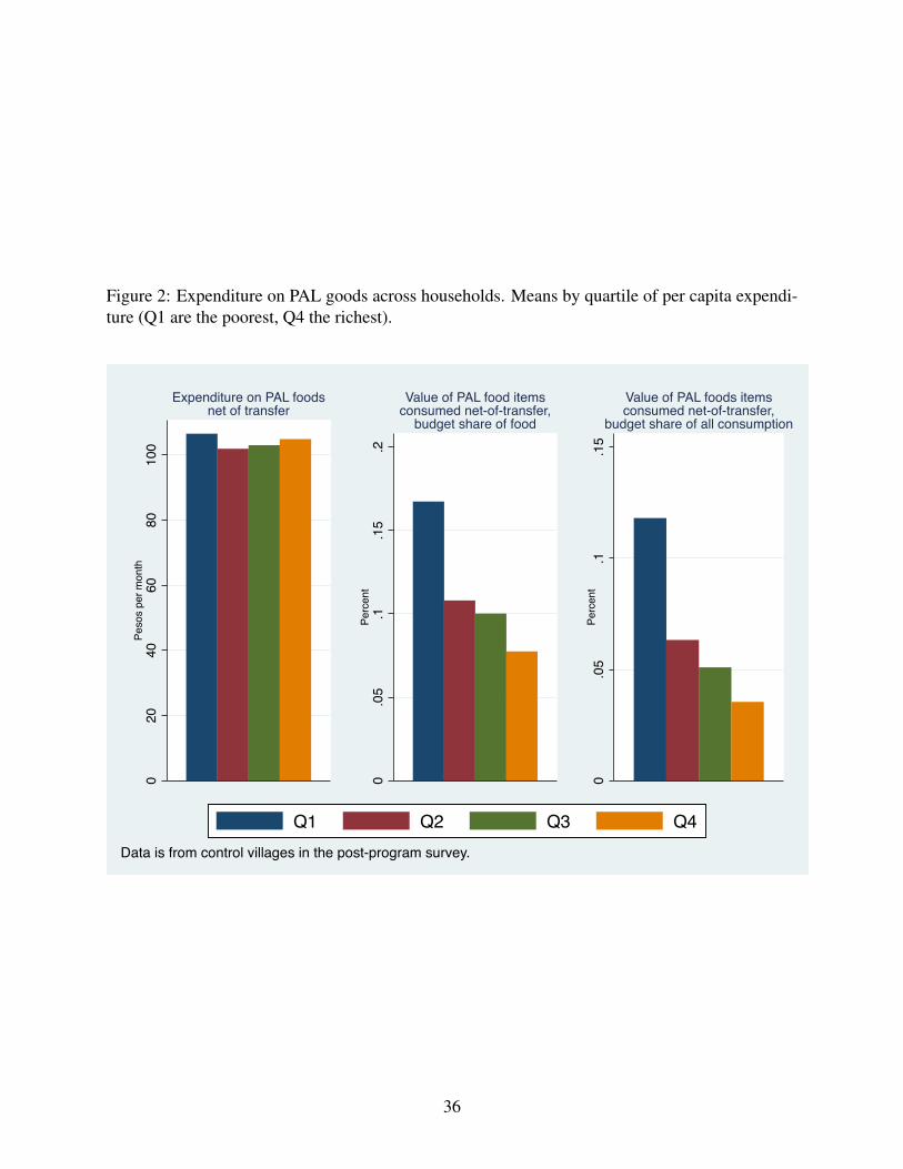
Figure 2: Expenditure on PAL goods across households. Means by quartile of per capita expendi-ture (Q1 are the poorest, Q4 the richest).

020

4060

8010

0Pe

sos

per m

onth

Expenditure on PAL foodsnet of transfer

0.0

5.1

.15

.2Pe

rcen

t

Value of PAL food itemsconsumed net-of-transfer,

budget share of food

0.0

5.1

.15

Perc

ent

Value of PAL foods itemsconsumed net-of-transfer,

budget share of all consumption

Data is from control villages in the post-program survey.

Q1 Q2 Q3 Q4

36

Table 1: Summary of PAL food box

Item TypeAmount per

box (kg)

Value per box (pre-program,

in pesos)

Calories, as % of total

box

Village change in supply (∆Supply)

(1) (2) (3) (4) (5)Corn flour basic 3 15.7 20% 1.00Rice basic 2 12.7 12% 0.61Beans basic 2 21.0 13% 0.29Fortified powdered milk basic 1.92 76.2 17% 8.62Packaged pasta soup basic 1.2 16.2 8% 0.93Vegetable oil basic 1 (lt) 10.4 16% 0.25Biscuits basic 1 18.7 8% 0.81Lentils supplementary 1 10.3 2% 3.73Canned tuna/sardines supplementary 0.6 14.8 2% 1.55Breakfast cereal supplementary 0.2 9.3 1% 0.90

Notes:(1) Value is calculated using the average of pre-treatment village-level median unit values. 10 pesos ≈ 1 USD. (2) ∆Supply measures the PAL supply influx into villages, relative to what would have been consumed absent the program. It is constructed as the average across all in-kind villages of the total amount of the good transferred to the village divided by the average consumption of the good in control villages in the post-period.(3) We do not know whether a household received canned tuna fish (0.35kg) or canned sardines (0.8kg); the analysis assumes the mean weight and calories throughout.(4) Biscuits are excluded from our analysis as post-program prices are missing.

37

Table 2: Baseline characteristics by treatment group

Control In-kind Cash(1)=(2)p-value

(1)=(3)p-value

(2)=(3)p-value

(1)=(2)=(3)p-value

Medianvillageunit-value,normalized 1.00 0.98 0.98 0.28 0.31 0.95 0.48(0.014) (0.012) (0.015)

Missingmedianvillageunit-value 0.14 0.14 0.13 0.98 0.65 0.60 0.86(0.017) (0.013) (0.018)

Observations(goodlevel) 282 576 306

Medianvillageunit-value,normalized 1.00 1.02 1.00 0.39 0.88 0.46 0.64(0.017) (0.016) (0.016)

Missingvillageunit-value 0.19 0.19 0.17 0.86 0.53 0.60 0.81(0.017) (0.014) (0.020)

Observations(goodlevel) 423 864 459

Medianvillageunit-value,normalized 1.00 1.02 1.00 0.23 0.98 0.18 0.30(0.015) (0.010) (0.013)

Missingvillageunit-value 0.24 0.24 0.24 0.97 0.96 0.99 1.00(0.018) (0.013) (0.017)

Observations(goodlevel) 2820 5760 3060

Missingmedianstoreprice 0.13 0.10 0.16 0.69 0.66 0.36 0.65(0.048) (0.034) (0.046)

Diconsastoreinthevillage 0.26 0.45 0.39 0.03** 0.16 0.51 0.08*(0.071) (0.049) (0.068)

Traveltimetonearestmarket(hours) 0.77 0.69 0.74 0.55 0.86 0.69 0.82(0.108) (0.076) (0.104)

Villagepopulation 682.83 580.39 543.90 0.29 0.21 0.70 0.42(79.653) (55.137) (75.648)

Numberofstores 0.00 13.21 12.96 0.00*** 0.00*** 0.52 0.00***(0.318) (0.224) (0.305)

Medianmonthsforwhichtransferswerereceived -- 1.82 1.80 -- -- 0.88 --(0.072) (0.098)

Observations(villagelevel) 47 96 51

Monthlypercapitaexpenditure(pesos) 570.48 535.06 529.51 0.31 0.26 0.85 0.50(29.02) (18.89) (21.77)

Food-producinghousehold 0.68 0.75 0.82 0.11 0.00*** 0.05* 0.01**(0.04) (0.02) (0.03)

Farmcosts(pesos) 413.76 664.92 784.65 0.03** 0.00*** 0.32 0.01**(82.46) (76.91) (93.22)

Farmprofits(pesos) 211.72 319.13 289.61 0.24 0.38 0.70 0.50(72.52) (56.80) (52.08)

Assetindex 2.24 2.18 2.27 0.78 0.87 0.59 0.86(0.16) (0.10) (0.13)

Indigenoushousehold 0.21 0.18 0.15 0.66 0.39 0.56 0.68(0.06) (0.03) (0.04)

Householdhasadirtfloor 0.32 0.31 0.32 0.77 0.95 0.70 0.92(0.04) (0.03) (0.03)

Householdhaspipedwater 0.65 0.57 0.50 0.23 0.06* 0.33 0.16(0.05) (0.04) (0.06)

Observations(householdlevel) 1291 2810 1473

Villagelevelcharacteristics

Householdlevelcharacteristics

Notes:***p<0.01,**p<0.05,*p<0.1(1)Standarderrorsinparentheses.Fornormalizedmedianvillageunitvaluesandhouseholdlevelcharacteristics,standarderrorsareclusteredatthevillagelevel.(2)Medianvillageunitvaluesarenormalizedwiththegood-specificcontrolgroupmeanandareimputedgeographicallyifmissing(seetext).(3)Traveltimetothenearestmarketisthetimeinhoursneededtotraveltoalargermarketthatsellsfruit,vegetables,andmeat.Itisconstructedasthevillagemedianofhouseholdself-reports.(4)Expenditureisthevalueofnon-durableitems(foodandnon-food)consumedintheprecedingmonth,measuredinpesos;sixhouseholdsaremissingexpendituredata.(5)Producerhouseholdsarethosethat,atbaseline,eitherauto-consumetheirproductionorreportplantingorreapingproduceorgrainorraisinganimals.(6)Farmcostsandprofitsarefortheprecedingyear.Samplesaretrimmedofoutliersgreaterthan3standarddeviationsabovethemedian(about1%ofobservations).(7)Theassetindexisthesumofbinaryindicatorsforwhetherthehouseholdownsthefollowinggoods:radioorTV,refrigerator,gasstove,washingmachine,VCR,andcarormotorcycle;twohouseholdsaremissingtheassetindex.(8)Ahouseholdisdefinedasindigenousifoneormoremembersspeakanindigenouslanguage.

Prices,basicPALgoods

Prices,allPALgoods

Prices,allgoods

38

Table 3: Price effects of in-kind and cash transfers

All#PAL#goods

Basic#PAL#goods#only

All#PAL#goods

Basic#PAL#goods#only

All#PAL#goods

Basic#PAL#goods#only

Outcome(=( price price price price ∆price ∆price(1) (2) (3) (4) (5) (6)

In=kind =0.037* =0.033 =0.036* =0.033 =0.062** =0.025(0.020) (0.020) (0.020) (0.020) (0.029) (0.024)

Cash 0.002 0.014 0.003 0.012 0.000 0.039(0.023) (0.027) (0.023) (0.026) (0.031) (0.029)

Lagged#normalized#unit#value 0.027 0.127***(0.021) (0.042)

ObservaMons 2,335 1,617 2,335 1,617 2,335 1,617

Effect&size:!In$kind!$!Cash $0.039** $0.047** $0.038** $0.045** $0.063** $0.064**

H0:!In$kind!=!Cash!(p$value) 0.02 0.04 0.03 0.04 0.02 0.02

Notes:##***#p<0.01,#**#p<0.05,#*#p<0.1

(1)#The#outcome#variable#in#columns#1=4#is#the#post=treatment#price;#it#varies#at#the#village=store=good#level.#It#is#

normalized#by#good;#the#price#is#divided#by#the#average#price#of#the#good#across#all#observaMons#in#the#control#group.

(2)#Lagged#normalized#unit#value#in#columns#1=4#is#the#village#median#unit=value,#imputed#geographically#if#missing#(see#

text),#normalized#using#the#good=specific#control#group#mean;#it#varies#at#the#village=good#level.

(3)#The#outcome#variable#in#columns#5=6#is#the#difference#between#the#normalized#post=treatment#price#(the#outcome#in#

columns#1=4)#and#the#lagged#normalized#unit#value#(the#baseline#price#measure#in#columns#1=2).

(4)#All#regressions#include#an#indicator#for#imputed#pre=program#prices#(see#text).

(5)#Standard#errors#are#clustered#at#the#village#level.#194#villages.

39

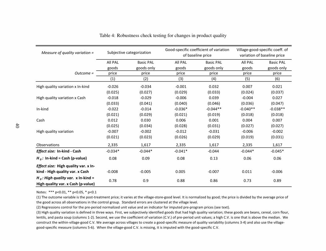
Table 4: Robustness check testing for changes in product quality

Measure of quality variation =

All PAL goods

Basic PAL goods only

All PAL goods

Basic PAL goods only

All PAL goods

Basic PAL goods only

Outcome = price price price price price price(1) (2) (3) (4) (5) (6)

High quality variation x In-kind -0.026 -0.034 -0.001 0.032 0.007 0.021(0.025) (0.027) (0.029) (0.033) (0.024) (0.037)

High quality variation x Cash -0.018 -0.029 -0.006 0.039 -0.004 0.027(0.033) (0.041) (0.040) (0.046) (0.036) (0.047)

In-kind -0.022 -0.014 -0.036* -0.044** -0.040** -0.038**(0.021) (0.029) (0.021) (0.019) (0.018) (0.018)

Cash 0.012 0.030 0.006 0.001 0.004 0.007(0.025) (0.034) (0.028) (0.031) (0.027) (0.027)

High quality variation -0.007 -0.002 -0.012 -0.031 -0.006 -0.002(0.021) (0.023) (0.026) (0.029) (0.019) (0.031)

Observations 2,335 1,617 2,335 1,617 2,335 1,617Effect size: In-kind - Cash -0.034* -0.044* -0.041* -0.044 -0.044* -0.045*

H 0 : In-kind = Cash (p-value) 0.08 0.09 0.08 0.13 0.06 0.06

Effect size: High quality var. x In-kind - High quality var. x Cash -0.008 -0.005 0.005 -0.007 0.011 -0.006 H 0 : High quality var. x In-kind = High quality var. x Cash (p-value)

0.78 0.9 0.88 0.86 0.73 0.89

Subjective categorizationVillage-good-specific coeff. of

variation of baseline priceGood-specific coefficient of variation

of baseline price

Notes: *** p<0.01, ** p<0.05, * p<0.1(1) The outcome variable is the post-treatment price; it varies at the village-store-good level. It is normalized by good; the price is divided by the average price of the good across all observations in the control group. Standard errors are clustered at the village level.(2) Regressions control for the pre-period normalized unit value and an indicator for imputed pre-program prices (see text). (3) High quality variation is defined in three ways. First, we subjectively identified goods that had high quality variation; these goods are beans, cereal, corn flour, lentils, and pasta soup (columns 1-2). Second, we use the coefficient of variation (C.V.) of pre-period unit values; a high C.V. is one that is above the median. We construct the within-village-good C.V. We average across villages to create a good-specific measure of quality variability (columns 3-4) and also use the village-good-specific measure (columns 5-6). When the village-good C.V. is missing, it is imputed with the good-specific C.V.

40

Table 5: Price effects based on duration of intervention

Outcome= price price price price

(1) (2) (3) (4)

In-kind -0.031 -0.056** -0.038 -0.056

(0.022) (0.026) (0.031) (0.035)

In-kindxAbovemedianlengthoftreatment -0.021 -0.011 -0.022 -0.018

(0.034) (0.035) (0.040) (0.043)

Abovemedianlengthoftreatment 0.004 -0.002 0.018 0.013

(0.028) (0.029) (0.033) (0.035)

In-kindxDevelopmentindex -0.047** -0.037

(0.022) (0.023)

Developmentindex 0.036** 0.039**

(0.015) (0.016)

Observations 1,818 1,665 1,258 1,150

AllPALgoods BasicPALgoodsonly

Notes:***p<0.01,**p<0.05,*p<0.1

(1)Theoutcomevariableisthepost-treatmentprice;itvariesatthevillage-store-goodlevel.Itisnormalizedbygood;

thepriceisdividedbytheaveragepriceofthegoodacrossallobservationsinthecontrolgroup.Standarderrorsare

clusteredatthevillagelevel.

(2)Regressionscontrolforthepre-periodnormalizedunitvalueandanindicatorforimputedpre-programprices(see

text).

(3)Lengthoftreatmentisdefinedasthevillagemediannumberofmonthsforwhichtransferswerereceievedprior

tothefollow-upsurvey.

(4)Thedevelopmentindexisthefirstprinicpalcomponentfromafactoranalysisofthefollowing4variables:(1)the

timerequiredtotraveltoalargermarketthatsellsfruit,vegetables,andmeat,(2)thedistancetotheheadofthe

municipality,(3)pre-programvillagemedianmonthlyexpenditureonnon-durables,and(4)thevillagepopulation.

41

Table 6: Heterogeneous price effects by level of village development, market integration, and supply-side competition

Below-median

development

Above-median

development

All

villages

Villageswith

marketpower

Villageswithout

marketpower

Below-median

pricecorrelation

Above-median

pricecorrelation

All

villages

All

villages

Outcome= price price price price price price price price price

(1) (2) (3) (4) (5) (6) (7) (8) (9)

In-kind -0.036 -0.033 -0.033 -0.048* -0.005 -0.060** -0.019 0.009 0.015

(0.031) (0.027) (0.021) (0.025) (0.021) (0.028) (0.028) (0.025) (0.035)

Cash 0.015 -0.007 -0.007 0.007 -0.005 0.002 -0.014 -0.036 -0.038

(0.032) (0.037) (0.032) (0.029) (0.026) (0.032) (0.032) (0.034) (0.041)

Developmentindexbelow-medianxIn-kind -0.006 -0.009

(0.018) (0.040)

Developmentindexbelow-medianxCash 0.018 0.006

(0.031) (0.048)

MarketpowervillagexIn-kind -0.039 -0.037

(0.036) (0.037)

MarketpowervillagexCash 0.029 0.027

(0.041) (0.044)

Pricecorrelationbelow-medianxIn-kind -0.039 -0.044

(0.041) (0.042)

Pricecorrelationbelow-medianxCash 0.022 0.022

(0.047) (0.048)

Observations 1,094 1,210 2,304 1,733 602 1,115 1,220 2,335 2,335

Effectsize: In-kind-Cash -0.051** -0.027 -0.026 -0.055*** 0.000 -0.063*** -0.006H0 : In-kind=Cash(p-value) 0.02 0.37 0.37 0.01 1.00 0.01 0.81Effectsize: Developmentindexbelow-medianxIn-kind-Developmentindexbelow-medianxCash -0.024 -0.015H0 : Developmentindexbelow-medianxIn-kind=Developmentindexbelow-medianxCash(p-value)

0.50 0.69

Effectsize: Pricecorrelationbelow-medianxIn-kind-Pricecorrelationbelow-medianxCash -0.061* -0.065*H0 : Pricecorrelationbelow-medianxIn-kind=Pricecorrelationbelow-medianxCash(p-value)

0.07 0.05

Effectsize:MarketpowervillagexIn-kind-MarketpowervillagexCash -0.067* -0.063*H0 : MarketpowervillagexIn-kind=MarketpowervillagexCash(p-value)

0.05 0.09

Notes:***p<0.01,**p<0.05,*p<0.1(1)Theoutcomevariableisthepost-treatmentprice;itvariesatthevillage-store-goodlevel.Itisnormalizedbygood;thepriceisdividedbytheaveragepriceof

thegoodacrossallobservationsinthecontrolgroup.Standarderrorsareclusteredatthevillagelevel.(2)Regressionscontrolforthemaineffectsoftheinteractiontermsreported,andforthepre-

periodnormalizedunitvalueandanindicatorforimputedpre-programprices(seetext).(3)Pricecorrelationisthecorrelationcoefficientofthepre-topost-programchangeinvillagepriceswiththe

pre-topost-programchangeinpricesinMexicoCityforallPALgoods,itvariesatthevillagelevel.(4)Thenumberofstoresisthenumberofstoresincludedinthebaselinepricesurvey;amaximumof

threestoresweresurveyedpervillage.(5)Thedevelopmentindexisthefirstprinicpalcomponentofafactoranalysisofthefollowing4variables:thetimerequiredtotraveltoalargermarketthatsells

fruit,vegetables,andmeat;thedistancetotheheadofthemunicipality;pre-programvillagemedianmonthlyexpenditureonnon-durables;andthevillagepopulation.

42

Table 7: Price effects for non-PAL goods

AllvillagesBelow-median

development

Above-median

developmentAllvillages

Outcome= price price price price

(1) (2) (3) (4)

In-kind 0.010 -0.006 0.024 0.024

(0.019) (0.030) (0.023) (0.023)

Cash 0.009 0.011 -0.0005 -0.001

(0.022) (0.032) (0.026) (0.026)

Developmentindexbelow-medianxIn-kind -0.030

(0.037)

Developmentindexbelow-medianxCash 0.012

(0.041)

Observations 10,648 4,699 5,832 10,531

Effectsize: In-kind-Cash 0.001 -0.017 0.025 0.025H0 : In-kind=Cash(p-value) 0.95 0.63 0.31 0.33

Effectsize: Developmentindexbelow-medianxIn-kind-Developmentindexbelow-medianxCash -0.042

H0 : Developmentindexbelow-medianxIn-kind=Developmentindexbelow-medianxCash(p-value)

0.33

Allnon-PALgoods

Notes:***p<0.01,**p<0.05,*p<0.1

(1)Theoutcomevariableisthepost-treatmentprice;itvariesatthevillage-store-goodlevel.Itisnormalizedbygood;thepriceis

dividedbytheaveragepriceofthegoodacrossallobservationsinthecontrolgroup.Standarderrorsareclusteredatthevillagelevel.

(2)Regressionsincludeall51non-PALgoodsandcontrolforthemaineffectsoftheinteractiontermsreported,aswellasforthepre-

periodnormalizedunitvalueandanindicatorforimputedpre-programprices(seetext).

(3)Thedevelopmentindexisthefirstprincipalcomponentofafactoranalysisofthefollowing4variables:(1)thetimerequiredto

traveltoalargermarketthatsellsfruit,vegetables,andmeat,(2)thedistancetotheheadofthemunicipality,(3)pre-programvillage

medianmonthlyexpenditureonnon-durables,and(4)thevillagepopulation.

43

Table 8: Effects for producer versus consumer households

Outcome = Farm

profitsFarm costs

ln(Expenditure per capita)

ln(Expenditure per capita)

Asset index

Asset index

(1) (2) (3) (4) (5) (6)

In-kind 143.87 134.01 0.115** 0.084(89.839) (119.511) (0.046) (0.075)

Cash 186.16* 345.32** 0.064 -0.040(106.082) (140.378) (0.052) (0.106)

Producer x In-Kind 0.001 -0.018 0.077 0.055(0.060) (0.046) (0.115) (0.088)

Producer x Cash 0.087 0.015 0.266* 0.229**(0.068) (0.051) (0.142) (0.109)

Producer -0.161*** -0.003 -0.308*** -0.007(0.050) (0.036) (0.092) (0.071)

Control for pre-period outcome? yes yes yes yes yes yesVillage FE yes yesObservations 4,924 5,038 5,534 5,534 5,571 5,571

Effect size: In-kind - Cash -42.29 -211.31* 0.050 0.124 H 0 : In-kind = Cash (p-value) 0.67 0.08 0.25 0.20

Effect size: Producer x In-Kind - Producer x Cash -0.086 -0.033 -0.189 -0.174*H 0 : Producer x In-Kind = Producer x Cash (p-value) 0.13 0.47 0.13 0.07

Notes: *** p<0.01, ** p<0.05, * p<0.1(1) Observations are at the household level. Standard errors are clustered at the village level. (2) Profits and costs are measured in pesos and they are for the preceeding year; samples are trimmed of outliers greater than three standard deviations above the median.(3) Producer is an indicator for households that, at baseline, either auto-consume their production or report planting or reaping produce or grain or raising animals.(4) Expenditure is the value of non-durable items (food and non-food) consumed in the preceding month, measured in pesos.(5) The asset index is the sum of binary indicators for whether the household owns the following goods: radio or TV, refrigerator, gas stove, washing machine, VCR, and car or motorcycle.

44

Appendix A. Price effects with imperfect competitionConsider a simple Cournot-Nash model with N identical stores and indirect market demand

for a homogenous good, p(Q;X). Total demand is Q = ∑ f q f = Nq where f = 1, ...,N indexesthe store. Each store faces constant marginal costs, C = cq. We assume that the demand curve isdownward sloping, i.e., ∂ p

∂Q < 0.Both an in-kind and cash injection can be represented by a shift in demand. A cash transfer has

only an income effect and is equivalent to a positive demand shift (for a normal good). An in-kindtransfer entails this income effect and an additional decrease in demand due to the external influxof goods; consumers receive some items for free from the government, so they now demand lessfrom local firms. In this model, such an exogenous change in demand is represented by a changein the demand shifter X , where we define ∂Q

∂X > 0.Stores maximize profits with respect to quantities taking others’ behavior as given (Nash equi-

librium):maxqΠ = p(Q)q− cq.

The first-order condition is p′q+ p− c = 0, which yields by substitution and differentiation:

p = c− Q(p;X)

N ∂Q(p;X)∂ p

≡ NεcNε−1

where ε ≡−∂Q∂ p

pQ is the price elasticity of demand.

The above equilibrium condition is useful for studying the effect of a shift in demand, e.g.,∂X > 0, on the equilibrium price. For the class of demand functions that are additive in X of theform Q = g(p)+X , we can immediately see that

d pdX

=− 1

N ∂g(p)∂ p

> 0

since ∂g/∂ p < 0 from the assumption of a downward-sloping demand curve. A simple examplein this class of demand curves is linear demand, e.g., Q = X−α p.

Thus, for any downward-sloping demand with an additive shifter, we can sign the price effectof a demand shift. For demand functions in this class, a cash transfer will lead to higher prices ofnormal goods and an in-kind transfer will lead to lower prices than a cash transfer, just as in thecase of perfect competition.

The price effect of a demand shift will in general be given by d pdX = −Nc dε

dX /(Nε − 1)2. Thesign of d p

dX , and hence the sign of the price effects of transfer programs, will depend on the signof dε

dX . For example, if transfers have a multiplicative effect on demand (e.g., Q = X p−α ), therewould be no price effects of transfers ( d p

dX = 0) since the elasticity of demand is independent of X .

45

Appendix B. Data appendix

VARIABLE CONSTRUCTION

Post-program pricesPost-program prices come from a survey of local stores; a maximum of three stores were

surveyed per village in each survey wave. Prices were collected in common units, for example theprice of a 150 milliliter container of yogurt, a “small” loaf of bread, or a kilogram of corn flour. Fornon-standard units, we converted prices to either kilograms (for solids) or liters (for liquids) usingconversion factors supplied by the Mexican government for non-standard units (e.g., a “small”loaf of bread weighs 0.68kg). In most specifications, post-program prices are normalized by thegood-specific mean in the control group.

Pre-program pricesThe main measure of the pre-program price is the village-median household unit value. House-

holds reported both expenditure and quantity purchased by good in a seven-day food recall survey,and the household unit-value is defined as the ratio of the two measures. For some goods in somevillages, there was no expenditure on a good by any household during the seven-day recall period,and therefore the village-median unit-value for that good is missing. In these cases, we impute thepre-program price using the median pre-program price in other villages within the same munici-pality (or within the same state in the few cases where there are no data for other villages in themunicipality). Among all PAL goods, we impute 18 percent of village-good observations; amongbasic PAL goods, we impute 14 percent of village-good observations.

An alternative pre-program price is the village median store price; we use the village medianas there is no store identifier in the data that would allow us to match stores between survey waves.When no price of a good is observed in a village pre-program, we impute this measure usingthe village median unit-value (19 and 16 percent of observations for all PAL goods and basicPAL goods, respectively). When the village median store price and the village median unit-valueare missing, we impute geographically as above (11 and 10 percent of observations for all PALgoods and basic PAL goods, respectively). For both of these measures of pre-program prices, wenormalize in most specifications using the good-specific mean in the control group.

Presence of a Diconsa storeWe identify the presence of a Diconsa store in a village from the names of stores that were

surveyed for their prices, coding this variable by hand. There could be false negatives if a Diconsastore was not one of the one to three stores surveyed.

Length of receipt of aidHouseholds self-reported to enumerators in the post-treatment survey whether they received

transfers in any of the preceding 24 months. Our village-level measure of the length for which aidwas received is the village median number of months for which transfers were received.

Variation in product qualityWe define the variation in the quality of PAL goods in two ways. First, we subjectively identi-

fied goods that had high quality variation; these goods include beans, cereal, corn flour, lentils, andpasta soup. Second, we calculate the village-good-specific coefficient of variation of pre-periodunit values, that is, the coefficient of variation among households in the village that purchased the

46

good. We also average this coefficient of variation across villages to create a good-specific versionof this proxy measure of quality variation.

Good- or village-specific influx of in-kind goods (∆Supply)∆Supply is a ratio that measures the size of the supply influx of in-kind goods into program

villages, relative to what would have been consumed in the absence of the PAL program. Weconstruct a village-good-specific measure: the village aggregate amount of a good that was orwould be transferred to the village (based on its eligibility rate) divided by the average consumptionof the good at baseline. In the descriptive statistics reported in Table 1, we report the averageacross in-kind villages of the actual supply influx, by good, where counterfactual consumption isthe average across control villages in the post period.

Development indexThe development index, defined at the village level, is constructed as the first principal com-

ponent of the following variables: pre-intervention average expenditures per capita, village pop-ulation, median self-reported travel time to a larger market that sells fruit, vegetables, and meat,and distance to the nearest municipality head. Expenditures per capital come from the PAL sur-vey, and village population comes from the Mexican census of 2005. For the self-reported traveltime, households were first asked if these fresh foods were sold in the village; if the answer wasno, they were then asked to state the time to get to the nearest market using their typical modeof transportation. We use the village median among households that report leaving the village topurchase fresh foods. The distance to the nearest municipality head is measured in kilometers andwas constructed using GIS software.

Market power indexWe classify villages into those where grocery shops have market power and those where they

do not. The measure of market power is the empirical implication of the model developed by At-tanasio and Pastorino (2015) relating the existence of price discounts for larger-quantity purchasesto the degree of imperfect competition in the market. When there is market power among sellers,there should be a negative within-village correlation between prices (unit values) and quantitiespurchased. We estimate the correlation between household unit values and and quantities con-sumed separately for each of the PAL villages using the pre-intervention data for the set of fooditems examined by Attanasio and Pastorino: rice, beans, sugar, tomatoes, and corn tortillas. Avillage is defined as having market power if the correlation coefficient is negative; in our sample75.2% of villages are classified as having market power.

Measure of opennessOur measure of the openness of a village economy is the correlation between pre-program

village prices and prices in the same year in national capital, Mexico City. We calculated good-specific Mexico City prices as the average good-specific Consumer Price Index (CPI) collectedby the Bank of Mexico between July of 2003 and July of 2004. Of the 60 food items in ourmain analysis, 9 do not have CPI data: soy, tomato paste, oats, mandarins, lard, canned chilis,atole, goat/lamb meat, and lentils. The openness measure is the correlation coefficient between theprices of 51 goods in a village and the same goods in Mexico City.

47

Total household consumptionExpendPC, or monthly per capita expenditure, is constructed as the sum of monthly household

food expenditure, non-food expenditure, and expenditure on food away from home, divided by thenumber of household members. Food expenditure is the value of food consumed; consumptionamounts were collected with a seven-day food recall module (converted to monthly amounts),covering 61 food items, and we use village median household unit-values (imputed geographicallyif missing) to value consumption. Non-food expenditure was reported at the monthly level andcovers 26 categories designed to capture the extent of non-durable, non-food expenditure (non-food consumption quantities were not collected). Weekly expenditure on food away from homewas self-reported by the household, and we convert to monthly amounts.

Farm production measuresWe use two measures of farm production: farm profits and farm costs. Both are self-reports

from the household surveys. Households were first asked whether any household member plantedor reaped produce or grain or raised animals in the past year. If yes, they were asked the total costsinvolved in these activities and then how much money was left after these costs had been paid (i.e.,farm profits). At baseline, among households that reported planting or reaping produce or grain orraising animals, 33 percent stated that farm costs were zero, and 85 percent stated that farm profitswere zero.

Producer household indicatorThe variable Producer equals one if, at baseline, a household either auto-consumed their pro-

duction or reported that, within the last year, any household member planted or reaped produceor grain, or raised animals. Auto-consumption data was collected for 61 food items in a seven-day food recall module. Households were asked to state the quantities consumed of each item,and how much of that consumption was from own production (auto-consumption). If a householdauto-consumed any positive amount of at least one good, we classify them as a producer.

Household asset indexWe construct an index of the durable assets a household owns from self-reports in the household

questionnaire. Households were asked if they owned each of the following six items: a radio orTV, a refrigerator, a gas stove, a washing machine, a VCR, and a car or motorcycle. We sum thenumber of items the household reports owning to create the variable Asset Index; thus, Asset Indexranges from zero to six.

QUALITATIVE SURVEYS OF FOOD STORES

We conducted two rounds of qualitative surveys of shopkeepers in a total of 52 villages in thestates of Veracruz, Oaxaca, and Puebla. The first round was in the spring of 2011 and included 16villages, 11 of which were PAL experimental villages and five are villages that were incorporatedinto the program after the experiment ended. The second was in the fall of 2015 and included36 villages, all of which were PAL experimental villages. In each village, a research assistantinterviewed several shopkeepers and asked a series of questions designed to learn about (1) theshape of the marginal cost curve and (2) the degree of competition. Specific topics included: howmany stores were in the village, how they procured supply, how they responded to unexpectedchanges in demand, and when they adjusted prices.

48

Appendix Table 1: There is no evidence of a differential impact across in-kind and cash villages infood expenditure away from home or non-food expenditure.

Outcome=

Foodexpenditureawayfromhome

percapita

Non-foodexpenditureper

capita

ln(Foodexpenditureawayfromhomeper

capita)

ln(Non-foodexpenditureper

capita)(1) (2) (3) (4)

In-kind 2.51 10.50 0.03 0.09*(3.86) (11.09) (0.13) (0.05)

Cash 2.29 22.40 0.00 0.10*(3.85) (13.83) (0.18) (0.06)

Observations 10,985 10,985 1,248 10,907

Effectsize: In-kind-Cash 0.23 -11.90 0.03 -0.01H0 : In-kind=Cash(p-value) 0.94 0.32 0.87 0.84Notes:

Notes: *** p<0.01, ** p<0.05, * p<0.1(1) Each column is a difference-in-differences regression of the outcome on treatment groups and survey waves. The In-kind and Cash coefficients reported are the interactions of those treatment groups with an indicator for the follow-up survey wave. (2) Standard errors are clustered at the village level.

49

Appendix Table 2: List of goods used in the analysis

Goods%used%in%analysisPAL%

goods

High%quality%varia7on

Goods%used%in%analysisPAL%

goods

High%quality%varia7on

1 tomato 31 oats2 onion 32 soy3 potato 33 chicken4 carrot 34 beef%and%pork5 leafy%greens 35 goat%and%lamb6 squash 36 seafood%(fresh)7 chayote 37 canned%tuna/sardines x8 nopale%(cactus) 38 eggs9 fresh%chili 39 milk%(liquid)10 guava 40 yogurt11 mandarin 41 cheese12 papaya 42 lard13 oranges 43 for7fied%powdered%milk x14 plantains 44 processed%meats15 apple 45 pastelillo%(snack%cakes)16 lime 46 soN%drinks17 watermelon 47 alcohol18 corn%tor7llas 48 coffee19 corn%kernels 49 sugar20 corn%flour x x 50 corn%or%potato%chips21 bread%rolls 51 chocolate22 sweet%bread 52 candy23 loaf%of%bread 53 vegetable%oil x24 wheat%flour 54 mayonnaise25 wheat%tor7llas 55 fruit%drinks26 dry%pasta%soup x x 56 consome%(broth)27 rice% x 57 powdered%fruit%drinks28 breakfast%cereal x 58 atole%(corn%based%drink)29 beans% x x 59 tomato%paste30 len7ls% x x 60 canned%chilis

Note:We%iden7fied%the%set%of%PAL%goods%with%high%quality%varia7on%prior%to%es7ma7ng%the%models%discussed%in%the%text.%%The%choice%of%goods%was%based%solely%on%our%knowledge%of%Mexican%food%consump7on%prac7ces%and%through%discussion%with%Mexican%colleagues.

50

Appendix Table 3: Additional baseline characteristics by treatment group

Control In(kind Cash

(1) (2) (3)

Number9of9household9members 4.78 4.64 4.61 0.409 0.369 0.849 0.619

(0.14) (0.10) (0.13)

Years9of9education9of9household9head 4.28 4.24 3.94 0.889 0.179 0.179 0.299

(0.18) (0.14) (0.17)

Household9has9running9water 0.65 0.57 0.50 0.239 0.06* 0.339 0.169

(0.05) (0.04) (0.06)

Household9has9an9outside9toilet 0.27 0.27 0.26 0.999 0.829 0.779 0.969

(0.04) (0.02) (0.04)

Household9has9electric9lights 0.82 0.90 0.88 0.169 0.309 0.799 0.369

(0.05) (0.02) (0.04)

Household9owns9their9own9home 0.83 0.83 0.83 0.859 0.789 0.899 0.969

(0.02) (0.01) (0.02)

In(home9food9consumption 316.33 298.67 288.73 0.319 0.129 0.489 0.309

(14.47) (9.48) (10.23)

Non(food9consumption 178.54 168.60 171.72 0.519 0.679 0.819 0.809

(12.64) (8.15) (10.19)

Out(of(home9food9consumption 14.78 11.70 9.46 0.199 0.03** 0.249 0.109

(2.00) (1.21) (1.46)

Consumption9of9PAL9in(kind9foods 45.08 45.66 45.98 0.819 0.729 0.879 0.949

(2.09) (1.24) (1.44)

Observations9(household9level) 1291 2810 1473

Notes:99***9p<0.01,9**9p<0.05,9*9p<0.19999Standard9errors9in9parentheses9are9clustered9at9the9village9level.

(1)=(2)

p(value

(1)=(3)

p(value

(2)=(3)

p(value

(1)=(2)=(3)9

p(value

Household)consumption)(monthly)pesos)per)capita)

Household)characteristics

51

Appendix Table 4: Main specification separately by PAL good

Corn%flour Rice Beans

Fortified%powdered%

milkPackaged%pasta%soup

Vegetable%oil Lentils

Canned%tuna%/%sardines

Breakfast%cereal

Outcome(=( price price price price price price price price price(1) (2) (3) (4) (5) (6) (7) (8) (9)

InIkind I0.012 I0.004 I0.042 I0.026 I0.070** I0.003 I0.012 I0.039 I0.062(0.019) (0.028) (0.033) (0.143) (0.034) (0.020) (0.061) (0.024) (0.099)

Cash I0.007 0.009 I0.024 0.113 0.035 0.036 I0.053 I0.023 0.027(0.023) (0.029) (0.038) (0.183) (0.083) (0.029) (0.068) (0.027) (0.121)

Lagged%normalized%unit%value 0.078 0.417*** 0.398*** I0.016 0.521*** 0.460*** 0.004 0.053** 0.003(0.052) (0.103) (0.074) (0.049) (0.137) (0.116) (0.067) (0.024) (0.027)

Observations 249 317 309 103 316 323 202 313 203

Effect&size:!In$kind!$!Cash $0.005! $0.014! $0.018! $0.140! $0.105! $0.040! 0.041! $0.016! $0.089!H0:!In$kind!=!Cash!(p$value) 0.80 0.62 0.55 0.28 0.18 0.12 0.47 0.47 0.30

Notes:%%***%p<0.01,%**%p<0.05,%*%p<0.1

(1)%The%outcome%variable%is%the%postItreatment%price;%it%varies%at%the%villageIstoreIgood%level.%It%is%normalized%by%good;%the%price%is%divided%by%the%average%price%of%

the%good%across%all%observations%in%the%control%group.%Colums%1I6%are%the%basic%PAL%goods,%columns%7I9%are%the%supplementary%goods.%%Standard%errors%are%

clustered%at%the%village%level.

(2)%Lagged%unit%value%is%the%village%median%unitIvalue,%imputed%geographically%if%missing%(see%text),%and%it%varies%at%the%villageIgood%level;%the%normalization%uses%the%

goodIspecific%control%group%mean.

(3)%Regressions%in%all%columns%include%an%indicator%for%imputed%preIprogram%prices%(see%text).

52

Appendix Table 5: Price effects of in-kind and cash transfers, alternative specifications

AllPALgoods

BasicPALgoodsonly

AllPALgoods

BasicPALgoodsonly

AllPALgoods

BasicPALgoodsonly

AllPALgoods

BasicPALgoodsonly

AllPALgoods

BasicPALgoodsonly

AllPALgoods

BasicPALgoodsonly

Outcome= price price price price ln(price) ln(price) price price price price price price(1) (2) (3) (4) (5) (6) (7) (8) (9) (10) (11) (12)

In-kind -0.037* -0.033 -0.026* -0.016 -0.037 -0.015 -0.037* -0.031 -0.032 -0.017 -0.027 -0.018(0.020) (0.020) (0.015) (0.014) (0.025) (0.022) (0.020) (0.021) (0.022) (0.023) (0.020) (0.021)

Cash 0.002 0.014 0.002 0.013 0.006 0.039 -0.004 0.003 0.002 0.015 0.014 0.018(0.023) (0.026) (0.018) (0.017) (0.028) (0.026) (0.022) (0.023) (0.023) (0.027) (0.023) (0.025)

Laggednormalizedunitvalue 0.034 0.128*** 0.101*** 0.276*** 0.025 0.149*** 0.022 0.091**(0.021) (0.042) (0.030) (0.040) (0.029) (0.056) (0.021) (0.043)

Laggednormalizedstoreprice 0.525*** 0.549***(0.048) (0.052)

Laggedln(unitvalue) 0.857*** 0.861***(0.025) (0.037)

Goodfixedeffects yes yesObservations 2,335 1,617 2,335 1,617 2,335 1,617 2,335 1,617 1,729 1,197 1,767 1,217

Effectsize: In-kind-Cash -0.038** -0.047** -0.029** -0.029** -0.044** -0.054** -0.033** -0.034** -0.034* -0.032 -0.040** -0.036*H0 : In-kind=Cash(p-value) 0.03 0.04 0.03 0.04 0.04 0.02 0.05 0.06 0.08 0.21 0.02 0.09

Excludingin-kindvillageswithoutclasses

Non-Diconsastoresonly

Notes:***p<0.01,**p<0.05,*p<0.1(1)Theoutcomevariableincolumns1-4and7-12isthepost-treatmentprice;itvariesatthevillage-store-goodlevel.Itisnormalizedbygood;thepriceisdividedbytheaveragepriceofthegoodacrossallobservationsinthecontrolgroup.Theoutcomeincolumns5-6isthelogarithmofthepost-treatmentstoreprice,withnonormalization.Standarderrorsareclusteredatthevillagelevel.(2)Laggednormalizedunitvalueisthevillagemedianunit-value,imputedgeographicallyifmissing(seetext),anditvariesatthevillage-goodlevel;thenormalizationofthisvariableusesthegood-specificcontrolgroupmean.(3)Laggedstorepriceisthevillagemedianstoreprice,imputedwiththevillagemedianunit-valueifmissing(seetext),anditvariesatthevillage-goodlevel;itisnormalizedusingthegood-specificcontrolgroupmeanthoseincolumns7and8includetwoimputationindicators(4)Laggedln(unitvalue)isthelogarithmofthevillagemedianunit-value,imputedgeographicallyifmissing(seetext);itvariesatthevillage-goodlevel.(5)Regressionsincolumns7-8areweightedatthegood-levelproportionaltothemeanexpenditureincontrolvillagesinthefollow-upsurvey.(6)Regressionsincolumns1-2and5-12includeoneindicatorforimputedpre-programprices;thoseincolumns3-4includetwosuchindicators(seetext).

Expenditureweightedregressions

53

Appendix Table 6: Tests of baseline balance by development index

Regressor=

Coefficient (s.e) Coefficient (s.e) Coefficient (s.e)

OutcomeMedianvillageunit-value,normalized 0.017 (0.030) 0.006 (0.039) -0.048 (0.043) 1,926Missingmedianvillageunit-value 0.058 (0.037) -0.073 (0.046) -0.150*** (0.055) 1,926

Medianvillageunit-value,normalized 0.038 (0.037) 0.008 (0.049) -0.019 (0.051) 2,889Missingvillageunit-value 0.011 (0.033) -0.091** (0.043) -0.164*** (0.051) 2,889

Medianvillageunit-value,normalized 0.029 (0.030) 0.004 (0.037) 0.002 (0.041) 19,260Missingvillageunit-value -0.090*** (0.032) -0.035 (0.040) -0.032 (0.044) 19,260

Missingmedianstoreprice -0.017 (0.059) -0.076 (0.090) 0.245* (0.137) 170Diconsastoreinthevillage -0.104 (0.134) -0.066 (0.173) 0.263 (0.205) 170Medianmonthsforwhichtransferswerereceived -- -- -1.026** (0.472) 0.011 (0.980) 170

Food-producinghousehold -0.191** (0.093) -0.073 (0.101) 0.085 (0.111) 1,979Farmcosts(pesos) -207.942 (296.626) 121.687 (350.373) 114.687 (358.265) 1,903Farmprofits(pesos) 279.562 (226.033) -164.342 (318.659) -201.309 (273.831) 1,867Assetindex 1.243*** (0.375) -0.034 (0.434) 0.173 (0.471) 1,978Indigenoushousehold -0.158 (0.149) -0.130 (0.167) -0.200 (0.177) 1,979Householdhasadirtfloor -0.151 (0.126) -0.179 (0.143) -0.191 (0.148) 1,979Householdhaspipedwater 0.150 (0.125) 0.096 (0.144) 0.146 (0.172) 1,979

Householdlevelcharacteristics

Notes:***p<0.01,**p<0.05,*p<0.1(1)Eachregressionalsoincludesindicatorsforcashandin-kindvillages.(2)Abovemediandevelopmentisanindicatorforavillagebeingabovethemedianofthefirstprinicpalcomponentofthefollowingfourvariables:thetimerequiredtotraveltoalargermarketthatsellsfruit,vegetables,andmeat;thedistancetotheheadofthemunicipality;pre-programvillagemedianmonthlyexpenditureonnon-durables;andthevillagepopulation.(3)Standarderrorsinparentheses.Fornormalizedmedianvillageunitvaluesandhouseholdlevelcharacteristics,standarderrorsareclusteredatthevillagelevel.(4)Medianvillageunitvaluesarenormalizedwiththegood-specificcontrolgroupmeanandareimputedgeographicallyifmissing(seetext).(5)Traveltimetothenearestmarketisthetimeinhoursneededtotraveltoalargermarketthatsellsfruit,vegetables,andmeat.Itisconstructedasthevillagemedianofhouseholdself-reports.(6)Expenditureisthevalueofnon-durableitems(foodandnon-food)consumedintheprecedingmonth,measuredinpesos;sixhouseholdsaremissingexpendituredata.(7)Producerhouseholdsarethosethat,atbaseline,eitherauto-consumetheirproductionorreportplantingorreapingproduceorgrainorraisinganimals.(8)Farmcostsandprofitsarefortheprecedingyear.Samplesaretrimmedofoutliersgreaterthan3standarddeviationsabovethemedian(about1%ofobservations).(9)Theassetindexisthesumofbinaryindicatorsforwhetherthehouseholdownsthefollowinggoods:radioorTV,refrigerator,gasstove,washingmachine,VCR,andcarormotorcycle;twohouseholdsaremissingtheassetindex.(10)Ahouseholdisdefinedasindigenousifoneormoremembersspeakanindigenouslanguage.

Prices,allgoods

Villagelevelcharacteristics

Abovemediandevelopment

In-kindxAbovemediandevelopment

CashxAbovemediandevelopment Obs

Prices,basicPALgoods

Prices,allPALgoods

54

Appendix Table 7: Household expenditure in cash villages, class attendees versus non-attendees.

Outcome(=(

Logs Levels Logs Levels Logs Levels Logs Levels(1) (2) (3) (4) (5) (6) (7) (8)

A3ended6classes 0.04 12.55 0.05 10.52 0.07 ;0.21 0.06 2.52(0.04) (27.72) (0.04) (15.74) (0.05) (3.25) (0.06) (18.76)

Lagged6outcome 0.42*** 0.56*** 0.38*** 0.42*** 0.30*** 0.42*** 0.34*** 0.51***(0.03) (0.06) (0.03) (0.06) (0.03) (0.06) (0.03) (0.05)

ObservaCons 1,257 1,257 1,257 1,257 1,252 1,257 1,235 1,257

Cash6villages6only

Notes:66***6p<0.01,6**6p<0.05,6*6p<0.1(1)6ObservaCons6are6at6the6household6level.6Sample6includes6all6PAL6eligible6households6in6cash6villages.(2)6Expenditure6is6the6value6of6goods6consumed6in6the6preceding6month,6measured6in6pesos.(3)6A6household6is6classified6as6a3ending6classes6if6they6report6a3ending6at6least6one6class6covering6topics6in6health,6hygiene,6or6nutriCon.(4)6Village6fixed6effects6included6in6all6regressions.6Standard6errors6clustered6at6the6village6level.

Total6expenditure6(food6+6non;food)6

per6capitaFood6expenditure6

per6capita

Expenditure6on6PAL6in;kind6food6items

per6capita

Non;food6expenditureper6capita

55

Appendix Figure 1: Trucks transporting PAL boxes

56

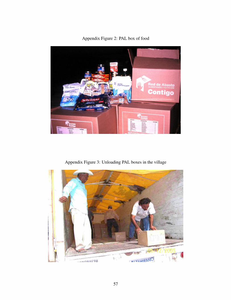
Appendix Figure 2: PAL box of food

Appendix Figure 3: Unloading PAL boxes in the village

57

Appendix Figure 4: Grocery shops in PAL villages

58

Appendix Figure 5: Villages in the PAL experiment

59