the potential of electricity storage by high temperature
TRANSCRIPT

The potential of electricity storage byhigh temperature heat storage within the
Ecovat context
Master Thesis
Chris Kwikkers
Department of Mechanical EngineeringSustainable Energy Technology Master Program
Energy Technology Group
Supervisor:Dr. Ir. Camilo Rindt
Examination committee members:Dr. Ir. Michel SpeetjensDr. Madeleine Gibescu
Eindhoven, June 2018


Contents
Contents iii
List of Figures v
1 Introduction 11.1 The need for electricity storage . . . . . . . . . . . . . . . . . . . . . . . . . . . . . 11.2 Problem definition and research question . . . . . . . . . . . . . . . . . . . . . . . . 21.3 Approach . . . . . . . . . . . . . . . . . . . . . . . . . . . . . . . . . . . . . . . . . 2
2 Energy storage background and techniques 32.1 Electricity storage . . . . . . . . . . . . . . . . . . . . . . . . . . . . . . . . . . . . 32.2 Current demand for flexibility . . . . . . . . . . . . . . . . . . . . . . . . . . . . . . 32.3 Current applications electricity storage . . . . . . . . . . . . . . . . . . . . . . . . . 62.4 Future markets electricity storage . . . . . . . . . . . . . . . . . . . . . . . . . . . . 82.5 Heat storage for electricity generation . . . . . . . . . . . . . . . . . . . . . . . . . 14
3 Electricity storage in the Ecovat context 163.1 Typical clients . . . . . . . . . . . . . . . . . . . . . . . . . . . . . . . . . . . . . . 163.2 Storage size and power requirements . . . . . . . . . . . . . . . . . . . . . . . . . . 173.3 Conversion methods . . . . . . . . . . . . . . . . . . . . . . . . . . . . . . . . . . . 183.4 Storage Module . . . . . . . . . . . . . . . . . . . . . . . . . . . . . . . . . . . . . . 213.5 General module design . . . . . . . . . . . . . . . . . . . . . . . . . . . . . . . . . . 24
4 Mathematical model 274.1 Organic Rankine Cycle . . . . . . . . . . . . . . . . . . . . . . . . . . . . . . . . . . 274.2 Storage Module . . . . . . . . . . . . . . . . . . . . . . . . . . . . . . . . . . . . . . 324.3 Concrete conduction model . . . . . . . . . . . . . . . . . . . . . . . . . . . . . . . 34
5 Simulation Results 455.1 Operating range of the conversion module . . . . . . . . . . . . . . . . . . . . . . . 455.2 Combined system . . . . . . . . . . . . . . . . . . . . . . . . . . . . . . . . . . . . . 465.3 Economic performance . . . . . . . . . . . . . . . . . . . . . . . . . . . . . . . . . . 54
6 Conclusions 566.1 General module design . . . . . . . . . . . . . . . . . . . . . . . . . . . . . . . . . . 566.2 Thermodynamic performance . . . . . . . . . . . . . . . . . . . . . . . . . . . . . . 576.3 Economic performance . . . . . . . . . . . . . . . . . . . . . . . . . . . . . . . . . . 576.4 Recommendations . . . . . . . . . . . . . . . . . . . . . . . . . . . . . . . . . . . . 57
Bibliography 59
iii

List of variables
Symbol Unit VariableAp [m] Pipe circumferenceAU [W/(m2/K)] Overall heat transfer coefficientC [kJ/K] Heat capacityc [kJ/(kg ·K)] Specific heat capacityd [m] DiameterE [J ] Energyf [−] Friction factorH [J ] Enthalpyh# [J/kg] Specific enthalpyh [W/(m2 ·K)] Heat transfer coefficientL [m] Lengthk [W/(m ·K)] Thermal conductivitym [kg] Massm [kg/s] Mass flown [−] Number of pipesP [W ] PowerQ [J ] Thermal energyR [m] Outer radiusr [m] RadiusS [J/K] Entropys [J/(K · kg)] Specific entropySP [−] Size parameterT [K] Temperaturet [s] Timeu [m/s] Bulk flow velocityV [m3] VolumeW [J ] Useful workx [m] Distance from inner diameterz [m] Distance from entrance pipeα [m2/s] Thermal diffusion coefficientε [%] Effectivenessη [%] Efficiencyρ [kg/m3] Density
iv

List of Figures
2.1 Electrical energy storage technologies [11] . . . . . . . . . . . . . . . . . . . . . . . 42.2 Installed capacity energy storage technologies,[5] . . . . . . . . . . . . . . . . . . . 42.3 Technological parameters of electricity storage technologies [21] . . . . . . . . . . . 52.5 Expected electricity price fluctuations for different ENTSOE scenarios [4] . . . . . 92.6 Spectral representation of expected power fluctuations in several scenarios [4] . . . 102.7 Needed storage capacity per timescale to meet supply/demand mismatch [4] . . . . 102.8 Overview of flexibility and capacity services with typical operating parameters [4] . 12
3.1 Example of a T-s diagram for an ORC . . . . . . . . . . . . . . . . . . . . . . . . . 203.2 Overview of ORC module prices[18] . . . . . . . . . . . . . . . . . . . . . . . . . . 213.3 Considered storage materials with properties [8] . . . . . . . . . . . . . . . . . . . . 223.4 Storage volume needed for the different storage materials, ORC . . . . . . . . . . . 233.5 Cost of storage material, heat exchanger and conversion module . . . . . . . . . . . 243.6 Overview of working fluid characteristics used in [7] . . . . . . . . . . . . . . . . . 26
4.1 Example of a T-s diagram for an ORC . . . . . . . . . . . . . . . . . . . . . . . . . 284.2 ORC plots for varying HTF input temperatures . . . . . . . . . . . . . . . . . . . . 304.3 Comparison of simulated thermal efficiency with literature values . . . . . . . . . . 324.4 Schematic representation of some cylindrical segments inside the bulk concrete . . 354.5 Schematic representation of concrete discretization . . . . . . . . . . . . . . . . . . 374.6 Temperature gradient for varying amounts of radius nodes . . . . . . . . . . . . . . 414.7 Time evolution of temperature gradient . . . . . . . . . . . . . . . . . . . . . . . . 434.8 Temperature distribution in concrete segment during charging . . . . . . . . . . . . 44
5.1 Thermal efficiency of sub-critical ORC for varying inlet temperatures . . . . . . . . 465.2 Schematic representation of ORC connected to the storage module . . . . . . . . . 475.3 Consumption profile used in discharge simulations, created from data from [16] . . 475.4 Supplied power and consumption profile during discharge simulation of starting setup 485.5 Thermal conversion efficiency of the ORC during discharge simulation . . . . . . . 495.6 Concrete segment temperature development during discharge . . . . . . . . . . . . 495.7 Supplied power and consumption profile during discharge simulation of base case . 515.8 Thermal conversion efficiency of the ORC during discharge simulation of base case 515.9 Inlet and outlet temperature of the ORC for during full power discharge . . . . . . 525.10 Thermal conversion efficiency of the ORC during full power discharge . . . . . . . 525.11 Sensitivity of the number of cycles needed to break even to fluctuations in energy
procurement costs . . . . . . . . . . . . . . . . . . . . . . . . . . . . . . . . . . . . 55
v


Chapter 1
Introduction
1.1 The need for electricity storage
The European Commission has introduced an energy roadmap to 2050 to combat climate change.This roadmap states that by 2050 the CO2 emissions of the European Union should be at 5% ofthe emissions of the year 1990 [6]. To achieve this it is necessary to shift from fossil fuel energysources to more renewable ones such as wind and solar. This shift to renewables has a profoundeffect on the European energy system. Due to the intermittent and unpredictable behavior ofrenewable energy sources, the stability of the electrical grid and reliability of energy supply areat risk. To combat these problems energy buffers can be implemented, absorbing excess energyand supplying energy when production is not sufficient. For this purpose, Ecovat has developed asensible heat storage system. Ecovat designs and manufactures underground seasonal heat storagetanks, using a passive, stratified water tank principle. The system is charged using heat pumpsand electric heaters during the spring and summer. Charging is done at times when electricitysupplied by the grid is abundant and cheap. By absorbing the excess electricity the Ecovat systemcan be used to balance the electricity grid and lower the curtailment of renewables. Due to itslarge size and good insulation, the heat can be stored for long periods of time with minimal losses.During the colder months the system is discharged to supply its customers with heat for centralheating and direct hot water purposes. Currently Ecovat is conducting validation experiments ontheir 70 MWh test location and developing their first full scale commercial project.
In the current configuration an Ecovat system is only able to store energy asymmetrically, ab-sorbing electricity and supplying heat. However, in light of the changing energy system Ecovat isinterested in the possibilities to incorporate symmetrical storage into their system. The ability tostore electricity symmetrically opens up a number of additional applications such as electric loadshifting and improving power quality and reliability.
Several techniques for stationary electrical energy storage are currently implemented in a vari-ety of applications. Most of these applications are used for emergency power or are used incombination with some sort of (renewable) energy generation. In these combinations the purposeof the electricity storage is to complement the power generation in the form of curve smoothingor expanding the time of operation. The performance of the different techniques varies greatly onaspects such as response time, power, storage capacity, operating temperature etc. Therefore, thetechnique which is used is strongly dependent on the desired application. In addition, boundaryconditions influence the efficiency or applicability of any given technique. An example of such aboundary condition is the availability of, or demand for, waste energy streams like saturated steamor low temperature heat. Other boundary conditions might limit certain techniques to locationswith very specific geographical attributes such as mountains or underground aquifers.
1

CHAPTER 1. INTRODUCTION
The initial focus of Ecovat was on short term storage of electricity, and utilize the short termfluctuations in electricity price and balance prices to achieve a feasible business case. After apreliminary analysis of the short term fluctuations in electricity prices it was concluded that, withcurrent prices and technology it was not economically feasible to implement electricity storage forshort term storage. Therefore it was decided to focus more on bulk energy storage for providingreliability of supply in an energy system with diminishing reliability.
Long term bulk electrical energy storage can be achieved using several approaches. Currentlythe most widely implemented form of electricity storage are: pumped hydro storage and elec-trochemical storage in the form of Lithium-ion batteries. In this report the focus will be onstoring electricity using high temperature heat storage (HTS). This focus was chosen because ofthe possible synergy HTS has with the existing Ecovat system.
1.2 Problem definition and research question
Due to the energy transition towards renewables the energy system is expected to change andwith it the need for new services is expected to develop. Due to the intermittent and unpredict-able behavior of renewable energy sources electricity storage is needed to maintain the currentreliability of supply. Furthermore, electricity storage can be used for services such as preventingcurtailment, power quality control and preventing congestion issues. The goal of this master thesisis to determine the possibilities for symmetrical electricity storage within the existing Ecovat byimplementing high temperature storage. This goal has led to the following research question:
How can symmetrical electricity storage in the form of high temperature storage be integratedwithin the Ecovat system to meet future energy system needs?
1.3 Approach
The research question focuses on the needs of the developing energy system therefore the first stepis to determine these needs. It is not an aim of this thesis to reach an economically competitivesolution, but the demands of a future energy system will be used to determine performance in-dicators for the system. To make this assessment future scenarios of the energy market will beanalyzed and possible applications for storage within these scenarios are determined.
To correctly identify the solution which has the highest potential in combination with the Eco-vat system a comparative study will be conducted. The different energy conversion and storageoptions are compared on several technical and economic aspects, with as key indicators thermalefficiency, profitability and practicality. To correctly asses the performance on these key indicatorsfirstly more fundamental aspects of the technology need to be determined. These include but arenot limited to:
- Storage capacity- Storage density- Discharging power- Discharging efficiency- Cost
After the configuration has been determined. a numerical model is constructed to model thedischarging behavior. A parameter study is conducted to assess the impact of parameter devi-ations on the performance of the system. Lastly the profitability of the system is assessed whencompared to alternatives and no electricity storage unit.
2

Chapter 2
Energy storage background andtechniques
In this chapter the developing need for large scale electricity storage is elaborated upon. Firstly,the current demand for services which can be performed by electricity storage are discussed, aswell as the way in which these are met now. Secondly, the effects of the changing energy systemon the need for electricity storage are discussed in further detail. Lastly, it is discussed how thesefactors impact the design of the system.
2.1 Electricity storage
Network scale Electricity storage has been used for decades to perform, amongst others, peakshaving and flexibility services. However, due to the rise of renewable energy sources interest hasgrown over the last number of years. This has led to many new projects being developed, andnew technologies are now being considered for these applications.
2.2 Current demand for flexibility
As mentioned in the introduction, the changing European energy system calls for novel techniquesto alleviate the problems caused by unpredictable and intermittent electricity sources. Even thoughthe scale on which these problems will occur is new, in essence the problems of imbalanced energysystems and a mismatch between supply and demand are not. Currently the flexibility servicesto deal with these problems are mainly performed by supply side management, fluctuating theoutput of power plants. However, fluctuating the output power does diminish the efficiency ofelectricity generation. Therefore demand side management is also implemented in the form of gridscale electricity storage.
The techniques used for grid scale electricity storage can be split into two categories: powerto power (P2P) and power to heat (P2H). P2P storage refers to systems which charge using elec-tricity and also supply electricity while discharging. P2H systems are also charged using electricitybut supply heat while discharging. The energy storage system proposed in this report is a P2Psystem, as the distinction between the categories is made in terms of system output not storageprinciple.
Currently P2P systems are used for flexibility operations such as power balancing and peak shav-ing for conventional power plants, frequency control and emergency power. Numerous differenttechniques exist to preform these operations, an overview of these is given in figure 2.1. Theextent to which the most prevalent of these technologies are implemented is shown in figure 2.2.
3

CHAPTER 2. ENERGY STORAGE BACKGROUND AND TECHNIQUES
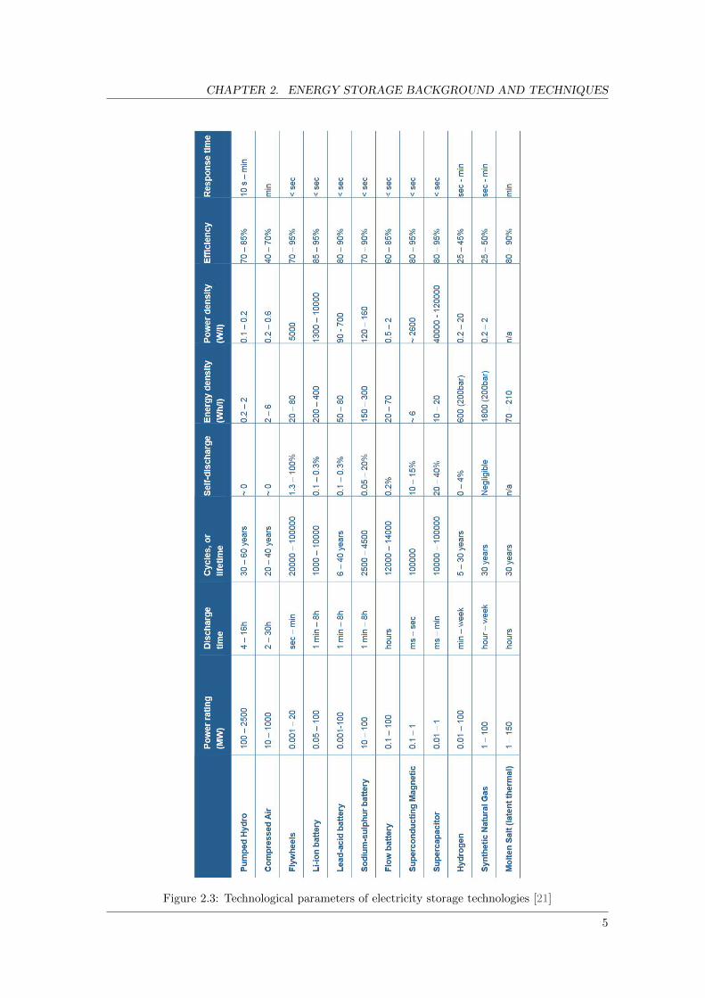
Different technologies are more suited for different applications depending on their performancecharacteristics. Among these characteristics power rating and rated discharge time are some ofthe most significant. These dictate what powers can be delivered and for how long, which is anindication of the total storage capacity. A summary of these parameters is given in figure 2.3. Thetechniques which are used most in current applications are discussed in the next paragraph.
Figure 2.1: Electrical energy storage technologies [11]
Figure 2.2: Installed capacity energy storage technologies,[5]
4
CHAPTER 2. ENERGY STORAGE BACKGROUND AND TECHNIQUES
Figure 2.3: Technological parameters of electricity storage technologies [21]
5

CHAPTER 2. ENERGY STORAGE BACKGROUND AND TECHNIQUES
2.3 Current applications electricity storage
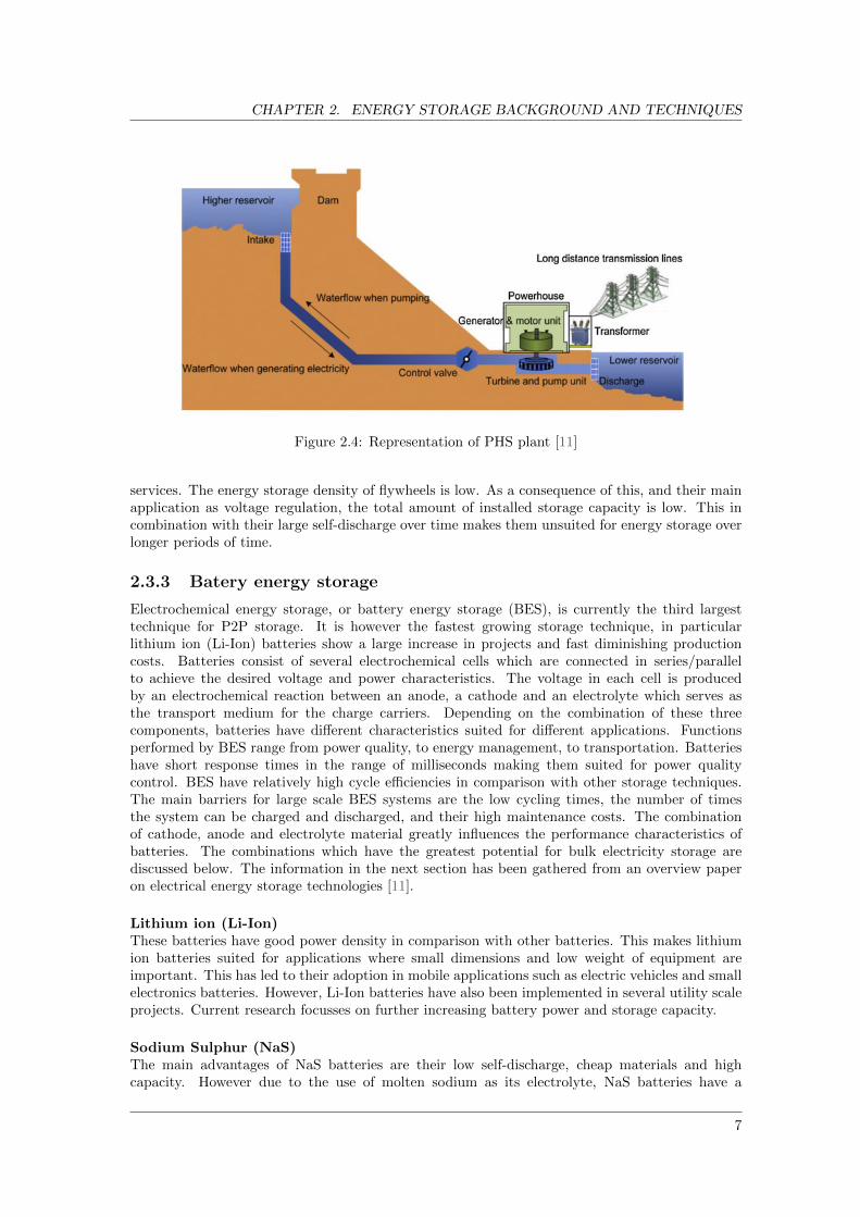
By far the most implemented form of P2P energy storage is pumped hydro storage (PHS). PHSsystems consist of two water reservoirs located at different heights, connected by a system ofpipes. During charging water is pumped from the lower reservoir to the higher reservoir, storingthe energy in the form of gravitational potential energy. During the discharging phase the waterin the higher reservoir is dropped to the lower reservoir. The high velocity falling water is fedthrough a turbine connected to a generator which generates electricity. A schematic representationof such an installation is shown in figure 2.4. The efficiency which can be achieved using PHSvaries between 70-80%. The total globally installed power of PHS exceeds 140 GW, accounting formore than 98% of P2P storage installed power. Roughly half of this installed power is installed inJapan, China and the US [22]. Because the amount of energy which can be stored in the systemscales with the height difference between the low and the high basin, a large height differential isdesired between the two, typically 200-300 meters. Furthermore, due to the low energy density ofPHS a large body of water is needed to store a functional amount of energy, typically 107 cubicmeters. PHS systems are therefore built in hilly or mountainous regions with (artificial) lakes,making the viability of such systems geographically limited. These constraints cause PHS systemsto have large investment costs and have long construction times. The investment costs are offsetby low operational costs, given that the plant is able to operate over a sufficiently long time span.PHS systems are primarily used to balance fossil fuel power plants and to provide peak power,they are therefore designed at large power levels, up to 3000 MW. Because the energy is storedin the form of gravitational energy self discharge is low making PHS suited for storage on longertime scales.
Even though most PHS projects were realized many years ago, the push for a less carbon in-tensive energy system has revamped industry interest. This has led to the development of newmethods such as salt water PHS. However, due to the impact that PHS has on the environmentin which it is implemented the suitability of PHS needs to be judged on a case to case bases.Therefore, the role that PHS will play in the future energy infrastructure will differ greatly percountry.[22].
2.3.1 Compressed air energy storage
The second largest P2P storage technique is compressed air energy storage (CAES). When usingthis technique air is compressed and stored at hight pressure. During discharge the compressedair is expanded over a turbine to generate electricity. Due to the low losses during storage thistechnique is especially suited for long term storage. The efficiency of the system can be improvedby storing the heat created during compression, and use this heat to improve the efficiency ofthe expansion process. The air can be stored in either: purpose built pressure vessels or existinggeological structures. However due to the high cost of the pressure vessels storage in existinggeological structures is preferred from an economic standpoint. This limits the number of possibleapplications of the technique. A variation on CAES is Liquefied Air Energy Storage (LAES),where the air is stored in its liquid form at atmospheric pressure. To achieve this the air needsto be cooled to -196 degrees centigrade and stored in an insulated tank. This allows for a verycompact storage tank, but to cool the air large additional equipment needs to be installed. Thismakes this option less suited for small scale applications.
2.3.2 Flywheel energy storage
At the other end of the spectrum lie technologies which are less suited for long term storage buthave very short response times. An example of such a technology is a flywheel which stores theenergy as rotational kinetic energy of a wheel spinning inside a vacuum chamber. Flywheels have avery short reaction time, meaning that they can start discharging quickly after the demand arises.This fast reaction time makes them especially suited for voltage/frequency regulation and ramping
6
CHAPTER 2. ENERGY STORAGE BACKGROUND AND TECHNIQUES
Figure 2.4: Representation of PHS plant [11]
services. The energy storage density of flywheels is low. As a consequence of this, and their mainapplication as voltage regulation, the total amount of installed storage capacity is low. This incombination with their large self-discharge over time makes them unsuited for energy storage overlonger periods of time.
2.3.3 Batery energy storage
Electrochemical energy storage, or battery energy storage (BES), is currently the third largesttechnique for P2P storage. It is however the fastest growing storage technique, in particularlithium ion (Li-Ion) batteries show a large increase in projects and fast diminishing productioncosts. Batteries consist of several electrochemical cells which are connected in series/parallelto achieve the desired voltage and power characteristics. The voltage in each cell is producedby an electrochemical reaction between an anode, a cathode and an electrolyte which serves asthe transport medium for the charge carriers. Depending on the combination of these threecomponents, batteries have different characteristics suited for different applications. Functionsperformed by BES range from power quality, to energy management, to transportation. Batterieshave short response times in the range of milliseconds making them suited for power qualitycontrol. BES have relatively high cycle efficiencies in comparison with other storage techniques.The main barriers for large scale BES systems are the low cycling times, the number of timesthe system can be charged and discharged, and their high maintenance costs. The combinationof cathode, anode and electrolyte material greatly influences the performance characteristics ofbatteries. The combinations which have the greatest potential for bulk electricity storage arediscussed below. The information in the next section has been gathered from an overview paperon electrical energy storage technologies [11].
Lithium ion (Li-Ion)These batteries have good power density in comparison with other batteries. This makes lithiumion batteries suited for applications where small dimensions and low weight of equipment areimportant. This has led to their adoption in mobile applications such as electric vehicles and smallelectronics batteries. However, Li-Ion batteries have also been implemented in several utility scaleprojects. Current research focusses on further increasing battery power and storage capacity.
Sodium Sulphur (NaS)The main advantages of NaS batteries are their low self-discharge, cheap materials and highcapacity. However due to the use of molten sodium as its electrolyte, NaS batteries have a
7

CHAPTER 2. ENERGY STORAGE BACKGROUND AND TECHNIQUES
high internal temperature of 574-624 K. This leads to high operating costs and the need for atemperature control system. Despite these difficulties NaS batteries are considered as one of themost promising candidates for bulk electrical energy storage. Currently there is one companywhich manufactures large scale NaS batteries for electrical energy storage which is situated inJapan. Production was halted briefly in 2012 after one of their battery systems had caught fireduring operation, production has resumed since then. Research is currently focused on increasingcell performance and lowering operating temperature.
Sodium Nickel Chloride (NaNiCl)The NaNiCl is similar to the NaS battery as they both use molten sodium as their electrolyte andboth operate at high temperatures. NaNiCl batteries have moderate performance with respect topower and storage density but require no maintenance, have very little self-discharge and goodpulsed power capabilities. Despite these advantages few companies have adopted and developedthe NaNiCl principle.
Flow battery energy storage (FBES)With conventional batteries the capacity and power of a cell are correlated. Therefore combinationssuch as a large capacity with low power are not practical which leads to expensive system andunused power capabilities. Flow batteries do not have this problem due to the use of liquidcathodic and anodic materials. This allows flow batteries to be adapted too specific applicationsand avoid unneeded costs. Furthermore, due to the fact that the materials are liquid they can bestored separately leading to very low self-discharge during storage.
2.4 Future markets electricity storage
How the demand for electricity storage will develop in the future is dependent on the developmentof the energy supply. To investigate this DNV-GL, an energy consulting company, in cooperationwith the TU Delft and Berenschot has used energy system scenarios made by the European networkof transmission system operators of electricity (ENTSOE) to predict future price fluctuationsand demand for flexibility. The results of this study have been outlined in the report RoadmapEnergystorage 2030 published in 2013 and the information in the following section is taken fromthat report [4]. The report outlines four possible scenarios for how the Dutch electricity systemmight adapt. Furthermore, the report analyses the expected demand for flexibility caused by thesefour scenarios and its impact on electricity prices. The four scenarios which are used in the reportare outlined below.
High sustainability CHP with 20 GW solar and windThis scenario is characterized by moderate implementation of solar and wind with flexible CHPplants to balance the system. This system requires low amounts of must run gas turbine balancingplants.
ENTSO-E vision 3 with 20 GW solar and windThis scenario contains the same amount implemented solar and wind but with fewer flexible CHPsto balance the system. This calls for a larger amount of must run gas turbine plants to balance thesystem. This leads to a large surplus of energy at times when solar and wind energy is abundant.
ENTSO-E vision 4+ with 30 GW solar and windSimilar to the previous scenario but with even more installed solar and wind. The increased shareof renewables aggravates the problems encountered in the previous scenario, large amount of mustrun gas turbines and large surpluses.
8

CHAPTER 2. ENERGY STORAGE BACKGROUND AND TECHNIQUES
Figure 2.5: Expected electricity price fluctuations for different ENTSOE scenarios [4]
ENTSO-E vision 4+- with 30 GW solar and windA variation on the Vision 4+ scenario with the addendum that fewer must run gas turbines areincluded. This leads to lower must run gas turbine power but a larger share of CHP plants.
The expected price fluctuations which arise from these scenarios are shown in figure 2.5. Fromthe figure it can be concluded that as the share of renewables increases the overall price decreaseas the price volatility increases. Note that the number of instances where the electricity priceapproaches zero increases as well along with the share of renewables.
Aside from the price fluctuations it was also studied at what intervals large fluctuations in powerwere expected to arise. As well as the amount of storage capacity needed to meet the storagedemand at each of these time intervals. This data is shown in figures 2.6 and 2.7. In these graphsthe ENTSO-E vision 4 scenario (the green line) is compared to the base load, as well as to scen-arios in which with other renewables are implemented. From the first graph it can be concludedthat all scenarios lead to larger fluctuations in power in comparison with the base load. A notableexception to this is the daily interval where the scenarios which employ a mix of renewables havesmaller fluctuations in comparison with the base case. The larger power fluctuations are in ac-cordance with the reasoning that larger shares of renewables will lead to larger power fluctuationson time scales not related to either human activity (daily) or meteorologically (annual cycles).This point is also reflected in the second chart where the demand for storage capacity deviatesfrom the base load especially on time scales between one day and one year.
2.4.1 Arbitrage
Due to the fluctuations in electricity price over time, storage can be used to store cheaply boughtelectricity until it can be sold for a higher price. This process of buying low and selling high issimilar to trading on the stock market and is referred to by a term borrowed from the stock market:arbitrage. Electricity can be bought or sold by pledging to consume or produce a certain amount
9

CHAPTER 2. ENERGY STORAGE BACKGROUND AND TECHNIQUES
Figure 2.6: Spectral representation of expected power fluctuations in several scenarios [4]
Figure 2.7: Needed storage capacity per timescale to meet supply/demand mismatch [4]
10

CHAPTER 2. ENERGY STORAGE BACKGROUND AND TECHNIQUES
of power for a number of Program Time Units (PTUs). Every hour is divided up into four PTUsof fifteen minutes each. Electricity units can be traded on the long term, day ahead, intraday andbalancing markets. DNV-GL used the scenarios and current pricing data to determine the impactof the different scenarios on the future electricity prices of the different markets.
Long term and day ahead marketsThese two markets refer to the buying and selling of PTU obligations before the producing andconsumption for that day has been locked in. The long term market refers to trading occurringmore than one day before the execution date, this time period can be as long as months or years.The day ahead market refers to the trade of energy to be delivered the next day, markets closethe day before. For the day ahead market the report concludes that the volatility increases forall scenarios, the most for scenarios with large shares of renewables. This increase in volatilitymanifests itself in an increase in the number of price fluctuations, not the magnitude of the pricedifferences. The most frequent price differential between hours was up to 20 EUR/MWh, thesetypically occurred on a time scale of six to twelve hours. This suggests a possibly profitable optionfor shorter charge/discharge cycles. One problem of trading on the day ahead market is thatbecause all bids must be done in advance, traders have little certainty when trading on longertime scales.
Intraday marketThe intraday market refers to the trading of energy within 36 hours before the energy is suppliedor demanded, the intraday is typically more volatile than the day ahead market. On the intradaymarket the volatility increases further in the scenario’s evaluated by DNV-GL, with both more andgreater price fluctuations. This makes it a more viable option for storage arbitrage. Furthermore,because traders can alter their bids up to five minutes before the dispatch time they have moreflexibility. However, price fluctuations in the intraday market are harder to predict leading tomore difficulties in planning this kind of arbitrage.
Balancing marketThe shortest term market is the balancing market, operating within one PTU before energy needsto be delivered. The short time span on which this market operates makes it the most volatileof all available markets with very large, albeit not many, price spikes. These price spikes can beused if the utilized storage technique is capable of responding quickly. DNV-GL concludes thatthe frequency and amplitude of spikes on the balancing market will decrease. This is caused bybetter prediction techniques and more international connections to absorb intermittent effects.
2.4.2 Flexibilty and ancillary services
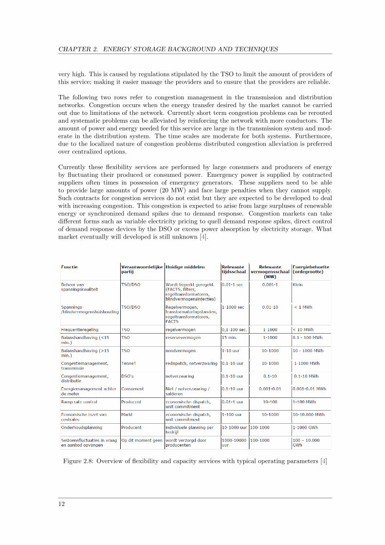
The report by DNV-GL has outlined the flexibility services which need to be performed alongwith the typical responsible party, current measures, time scale, power level and energy quantityin 2.8 (Dutch). In the table the abbreviations TSO and DSO stand for Transmission System Op-erator and Distribution System Operator respectively and TenneT is the TSO for the Netherlands.
Several categories of flexibility services can be identified. The top two rows outline services asso-ciated with power quality control and are characterized by short response times, low to moderatepower and small to moderate energy quantities. These processes are operated almost continuouslyto ensure constant power quality.
The next three rows are concerned with balancing, reserve and emergency power. When thepower committed to producing power and consuming power do not match at any given moment,the TSO contracts more consumers or suppliers to balance the load. The time scale at which thesesuppliers or consumers can react to the request of the TSO determines for which of the servicesthey can be contracted. Also note that the minimum needed power for these three services is also
11
CHAPTER 2. ENERGY STORAGE BACKGROUND AND TECHNIQUES
very high. This is caused by regulations stipulated by the TSO to limit the amount of providers ofthis service; making it easier manage the providers and to ensure that the providers are reliable.
The following two rows refer to congestion management in the transmission and distributionnetworks. Congestion occurs when the energy transfer desired by the market cannot be carriedout due to limitations of the network. Currently short term congestion problems can be reroutedand systematic problems can be alleviated by reinforcing the network with more conductors. Theamount of power and energy needed for this service are large in the transmission system and mod-erate in the distribution system. The time scales are moderate for both systems. Furthermore,due to the localized nature of congestion problems distributed congestion alleviation is preferredover centralized options.
Currently these flexibility services are performed by large consumers and producers of energyby fluctuating their produced or consumed power. Emergency power is supplied by contractedsuppliers often times in possession of emergency generators. These suppliers need to be ableto provide large amounts of power (20 MW) and face large penalties when they cannot supply.Such contracts for congestion services do not exist but they are expected to be developed to dealwith increasing congestion. This congestion is expected to arise from large surpluses of renewableenergy or synchronized demand spikes due to demand response. Congestion markets can takedifferent forms such as variable electricity pricing to quell demand response spikes, direct controlof demand response devices by the DSO or excess power absorption by electricity storage. Whatmarket eventually will developed is still unknown [4].
Figure 2.8: Overview of flexibility and capacity services with typical operating parameters [4]
12

CHAPTER 2. ENERGY STORAGE BACKGROUND AND TECHNIQUES
2.4.3 Profitability and regulatory boundaries
A major issue affecting the wider implementation of electricity storage systems is the higher coststhey add to the already expensive transmission and distribution networks or deployment of renew-able energy systems. This often renders them uneconomical if used for a single application whencompared with alternative conventional solutions.
Therefore it is important for incumbent technologies to be useful for multiple applications sothat, if properly managed, multiple income streams can be generated. Technologies which arecapable of offering several services combine instantaneous to fast response with moderate stor-age capacity or moderate response with large storage capacity. This allows the technologies tocompete on both the flexibility and energy markets or the energy and capacity markets respectively.
For energy applications the main barriers are as follows. The predominant mechanism to profitfrom energy applications is through energy arbitrage. How much money can be made throughthis mechanism is directly dependent on the short term price difference between spot prices forelectricity. These prices can be depressed by large bids from large suppliers. This makes it moredifficult for small suppliers to correctly forecast prices [11]. Due to the European legislation forcingthe electricity systems in member states to be unbundled difficulties arise when flexibility servicesare to be performed with electricity storage. Due to the nature of flexibility services it entailsthe buying and selling of electricity while strictly being a part of the distribution system. Thisresults in the stacking of fees for suppliers and consumers and legal problems regarding supplyingelectricity whilst supporting the DSO.
For capacity applications TSOs dictate a minimum power capacity and operation time for ca-pacity suppliers. This is done to limit the amount of suppliers and make it easier to guaranteereliability of supply. However, the powers demanded by the TSOs are in the order of megawattswhich is not realistic for decentral storage applications. Until now these regulatory boundariesmake it very hard for suppliers of storage capacity to enter the market. Industry parties are lob-bying for these rules to be changed. However, whether or not these regulations will be changed isuncertain and lies outside the scope of this report.
2.4.4 Implications for the Ecovat system
From the report by DNV-GL it can be concluded that trading on the long term market provesmost promising for storage times between 2-3 days. On these time scales relatively large price fluc-tuations up to 50-60 EUR/MWh are expected due to meteorological effects. Longer storage timesdo not seem profitable due to lower price differentials and the possibility for fewer charge/dischargecycles.
As mentioned before the balancing market provides the largest price differences. These are, how-ever, by their nature not predictable and short lived. Therefore only very fast acting storagemethods such as flywheels and batteries are feasible.
The main focus of the Ecovat electricity storage module is to form a complete energy storagesystem in combination with the usual heat storage unit. This system would allow the Ecovatsystem to manage the total energy supply of its connected consumers. By bundling the electricitydemand of all the consumers it becomes possible to provide emergency power from storage in caseof an outage, a service not yet provided in the current electricity market. The potential monetaryvalue of such a service is unknown and has not been investigated in a residential context. Howeverwith the increase of renewable energy sources in the energy mix the reliability of energy supplymight deteriorate, and more self-sustaining local grids might be desirable. Furthermore, due to theexpected increase in installed solar PV capacity in the residential sector, local storage of electricitywill prove more profitable and maybe even essential for distribution grid stability.
13

CHAPTER 2. ENERGY STORAGE BACKGROUND AND TECHNIQUES
2.5 Heat storage for electricity generation
As mentioned in the introduction, this thesis particularity focuses on electricity storage by storingit in the form of high temperature heat. In the next section some background information aboutconverting electricity to heat and vice versa is provided. After which, this information can becombined with the previous sections to determine possible storage configurations.
Heat can be converted into electricity by the use of heat engines, such as steam turbines, incombination with a generator. The maximum efficiency with which thermal energy can be conver-ted into electricity is directly dependent on the temperature difference driving the heat engine. Inpractice this means that higher input temperature leads to greater conversion efficiency. Electri-city production from heat storage is therefore mostly applied in contexts where high temperatureheat is readily available, such as concentrated solar power (CSP) plants. CSP plants reach tem-peratures of several hundred degrees centigrade, and can therefore convert the heat to electricitywith reasonable efficiency.
The Ecovat system does not produce such high temperatures so these would have to be pro-duced using electric heaters. However, HTS has a possible synergy with the Ecovat system. Oneof the drawbacks of HTS is high energy losses to the ambient due to an increased temperaturedifferential. By placing the storage within the Ecovat vessel the temperature gradient could be di-minished and any remaining losses would be absorbed by the low temperature vessel. This meansthat the cooling of the HTS would only lead to a loss of exergy and not a loss of energy. Becauseof this reason HTS is considered as a possible means for electricity storage in the Ecovat concept.
Another option is to use technologies currently implemented in waste heat to electricity con-version processes. These processes operate at lower temperatures which would make the energyeasier to store whilst maintaining efficiency. These processes do require more capital investmentsper kW installed and are harder to scale than high temperature installations.
In any case the HTS system will consist of a storage module and two conversion modules, fromelectricity to heat and vice versa. Technical possibilities for each of the conversion steps are dis-cussed below. The information used in the next section regarding storage principles is taken fromtwo studies outlining the state of the art in HTS [8] [13].
2.5.1 Power to heat
Heat pumps are used to maximize the efficiency of the conversion from electricity to heat whilecharging the water vessel. The temperatures needed for HTS cannot be achieved with heat pumps.Electric heaters can reach these temperatures and depending on the configuration electric boilersor immersion heating elements are preferred.
2.5.2 Heat to power
As mentioned before conversion from heat to power is usually done by connecting a heat engine toa generator. The predominantly used heat engine is a steam turbine which is the preferred heatengine for conventional fuels such as coal. To prevent nucleation of the water inside the turbinewhilst having sufficient expansion over the turbine, the inlet temperatures and pressures neededfor steam turbines are quite high. These temperatures can routinely be reached using fossil fuelssources but are harder to achieve using renewable energy sources.
To convert heat from lower temperature sources into electricity an Organic Rankine Cycle (ORC)can be used. ORCs operate on the same principle as the steam turbines, i.e. the Rankine cycle,but do not use water as the working fluid. By using another working fluid, such as CO2 whichhas a different saturation curve, higher efficiencies can be achieved whilst using lower operating
14

CHAPTER 2. ENERGY STORAGE BACKGROUND AND TECHNIQUES
temperatures. ORC generators are currently used to utilize lower temperature heat sources suchas geothermal heat or waste heat sources. A third possible heat engine is the Stirling engine.This technology can reach high efficiencies at low temperatures and can use heat from a largevariety of sources. This makes the Stirling engine especially suited for waste heat sources, andthe technology has seen a surge in interest as the demand for energy saving measures increases.The applications have however been limited to relatively small scale installations due to difficultieswith scaling the technology.
2.5.3 Sensible heat storage
Sensible heat storage refers to storing the thermal energy in a material which increases in temper-ature as it is charged. Many different heat storage techniques and materials are used for sensibleheat storage. The three most commonly used material categories are molten salts, thermal oilsand concretes. The general attributes of these three categories are elaborated upon below butwithin these categories large variations may occur for specific materials.
Storage techniques can be divided into several categories, the largest of which are active andpassive storage. Active heat storage means that the storage material itself is pumped through aheat exchanger during charging and discharge. Passive storage indicates that a heat exchangerwhich charges the storage is placed in the storage material and the storage is charged by running aheat transfer fluid (HTF) through the heat exchanger. Active storage can be subdivided into directand indirect storage. This distinction refers to whether the heat storage material is also the HTF(direct) or that another HTF is used to transport the heat from the source to the storage (indirect).
Molten salts have been popular as a heat storage material due to fact that they are liquid atatmospheric pressure when heated to high temperatures, have good heat capacity and thermalconduction and can be relatively cheap. Furthermore, molten salts are compatible with the op-erating requirements of steam turbines. One major drawback of using molten salts is their highfreezing temperature. One of the most used commercial salts freezes at 224 degrees centigrade.Therefore the storage and any pipes containing the salt must be kept at high temperatures toavoid solidification. Furthermore, the high temperatures needed for storage lead to higher lossesduring operation.
Mineral and synthetic oils do not freeze at lower temperatures but also lack some of the be-neficial attributes of molten salts. They have lower thermal conductivity and volumetric specificheat capacity leading to larger storage requirements and lower charge and discharge rates. Fur-thermore, thermal oils need to be pressurized to reach the same temperatures as molten salts. Thecost of thermal oils varies greatly with composition and can be very high. Some of these costsmight be mitigated by using mixed medium tanks to lower the amount of oil needed.
Other novel approaches to single tank HTS aimed at improving stratification or reducing costs arefloating stratification barriers and immersed steam generators [3].
Concrete is a promising heat storage material due to its low price, good thermal conductivityand abundance of materials. Because concrete is a solid only passive storage is possible and there-fore heat exchangers need to be integrated in the storage material.In the next chapter the findings regarding the electricity markets and conversion technologies areapplied to the Ecovat context.
15

Chapter 3
Electricity storage in the Ecovatcontext
In the previous chapter the changing markets for electricity storage have been discussed alongwith possible revenue generating configurations. Due to the goal of this thesis to implement theelectricity storage module in the existing Ecovat system, the typical parameters of this systemshould be taken into account. This chapter discusses the parameters of the Ecovat system, itstypical clients and what these parameters mean for the electricity storage module and conversionmodule.
3.1 Typical clients
The Ecovat energy storage system is a large scale sensible thermal energy storage module meantfor seasonal heat storage. When storing energy in the form of sensible heat, large scale storagemodules are preferred over smaller ones. This is due to the fact that the energy storage capacityscales with the volume of the storage unit and the losses scale with the outer surface area of themodule. However, when larger storage modules are used, more consumers are connected to onestorage site. This increases the average distance between storage and consumer, and consequentlytransport losses increase. Therefore, the advantages of large scale storage need to be balancedwith additional transportation losses caused by more spread out customers. These factors limitthe applications for which an Ecovat of a particular size is suitable, and therefore Ecovat focuseson three distinct market sectors. These sectors are: the built environment, greenhouse food pro-duction and heat grids. In all of these application the Ecovat system which is implemented isroughly the same, but some details differ between the applications.
The built environment sector refers to larger scale housing projects with one contracted heatsupplier. This means that all the heat demands of the entire housing project are met by onesupplier, allowing the investment in a shared large scale storage such as an Ecovat. Examples ofthese are large apartment complexes, campuses of different kinds and public housing projects.
Greenhouse agriculture requires a large amount of heat to make sure the crops can still be grownduring the winter. Due to the large heating demand one greenhouse farmer has, an Ecovat systemcan prove profitable when connected to a single consumer.
The last sector is district heating networks connected to a heat source, for example waste heator geothermal heat. The advantage of installing an Ecovat system in the heating network is thatmore consumers can be connected to the same heat source. Due to load shifting the peak heatingproduction required during winter is lowered, allowing for a more stable production profile andmore connected consumers.
16

CHAPTER 3. ELECTRICITY STORAGE IN THE ECOVAT CONTEXT
3.2 Storage size and power requirements
As discussed in the previous chapter to achieve a positive business case with electricity storage thestacking of services is crucial. Therefore the storage system should be dimensioned in such a waythat multiple services can be performed by the same system. This means for example that powerdelivery capacity might be over dimensioned for pure arbitrage services to also allow for balancingservices. Furthermore, due to the fact that Ecovat is already engaged in heat storage and supplyservices for its clients, integration of electricity storage services would result in a complete energysupply service for its connected consumers. However, providing this service demands differentdesign parameters than both arbitrage and services.
In the following section the technical parameters associated with these different services are dis-cussed. This is done to determine what specifications the electricity storage module should haveto serve its intended use. The application used to preform this analysis is the scenario where theEcovat is used in the built environment, serving a number of contracted consumers. The Ecovatsystem provides heating and backup power for these consumers with the possibility of performingarbitrage and flexibility services.
3.2.1 Backup power
The thermal storage capacity of the Ecovat systems go up to 4.5 MWh of thermal energy to beused for space heating and hot water supply. On an annual basis a storage of this size is able toprovide heat storage services for around 300 dutch households. The aim of the electricity storageunit is to be able to provide two days of emergency electricity for its connected consumers. Theaverage annual electricity consumption of one dutch household is 3500 kWh. The energy neededto provide 300 households with electricity for up to two days is therefore approximately 5750kWh, not accounting for storage and conversion losses. The power consumed by a typical Dutchhousehold peaks at just below 1 kW for terraced housing connected to district heating systems[10]. The total electric power output of the system should therefore be at least 300 kW to meetthe peak demands of the connected consumers.
3.2.2 Flexibility services
The relevant power, storage capacity and timescales required by different flexibility and capa-city services differ greatly between services. The parameters required for these services shouldby comparable to the parameters needed for backup power, to efficiently incorporate the flexibil-ity services in the electricity storage system. An overview of these parameters is given in figure 2.8.
The power and energy storage parameters for backup power, 300 kW and 5750 kWh, align bestwith the parameters of: voltage control, congestion management in the distribution grid and con-sumer energy management. Whether the response time of the energy storage module is suitedfor voltage control is unlikely. This is due to the fact that to preform voltage control servicesvery fast reaction times are required, i.e. within one second. Techniques capable of reacting thatquickly, for example flywheels, do not have significant storage capacity and are therefore not suitedfor electricity storage purposes. These techniques are therefore not considered for the electricitystorage module, and voltage control services can consequently likely not be performed.
The one MW minimum power requirement for many of the flexibility services is currently dic-tated by the regulatory framework stipulated by the TSO ’TenneT’. This is done to limit thenumber of suppliers able to participate in this market, which makes it easier for the TSO to man-age the reliability of its flexibility service providers. A different regulation requires the balancingservice providers to balance their energy ledgers. This means that on a daily basis each provideris required to conform to their pledged net consumption or production of electricity, or else en-dure a fine. These regulations make it harder for energy suppliers with limited power and energy
17

CHAPTER 3. ELECTRICITY STORAGE IN THE ECOVAT CONTEXT
management capabilities to enter the flexibility market. It has been proposed to remove one orboth of these regulations, which would open up the possibility for more players, such as Ecovat,to offer flexibility services. This lifting of regulations could help shift the flexibility services awayfrom the fossil fuel power plants, towards smaller more sustainable providers. However, because ofthe uncertainty regarding these regulatory changes, one cannot assume these services will providea reliable source of revenue. Therefore the design of the system is not altered to accommodate theperformance of these services.
In the case that the balancing requirement but not the power requirement is lifted, the Eco-vat system could preform balancing services by consuming more power to convert to heat. In thecase that both regulations are lifted electricity could be supplied back to the grid from the electri-city storage. However, whether this makes economic sense is strongly dependent on the balancingtariff offered by the TSO. This is due to the conversion losses associated with storing the energy.The value of the lost energy needs to be compensated by the difference between tariffs charged forconsuming and supplying the energy. On the balancing market the tariff is dictated by how muchthe realized supply and demand of electricity differs from the planned supply and demand. Thesetariffs can make the price of electricity skyrocket when consuming at the time of a shortage. Onthe other hand the price of energy can also become less then zero when there is an excess of energy.The tariffs are determined in time slots of 15 minutes. An estimation of how many time slots wereprofitable in the previous year, for either buying or selling at different conversion efficiencies, hasbeen conducted. The results of these estimations suggest that only a very limited number of timeslots would prove profitable. Therefore it is not likely that the electricity storage would be usedfor balancing services in the scenario that the TSO demands balancing of the energy ledger.
3.3 Conversion methods
To store electricity in the form of heat the energy needs to be converted from electricity to heatand back. To preform these conversions several technologies exist. The conversion from power toheat can be done using resistive heating at an efficiency approaching 100 %. Using heat pumpseven higher conversion efficiencies can be achieved. However, the output temperatures of suchheat pumps are limited. The conversion from heat to power is usually done by connecting a heatengine to a generator. Several heat engines can be used for this step, three of these are discussedbelow. In the next subsections these three technologies will be compared with respect to theirefficiency, price and practical applicability in the Ecovat setup.
The predominantly used heat engine is a steam turbine which is the preferred heat engine forconventional fuels such as coal. Steam turbines have high efficiency at high temperatures and canbe used at large scale. To prevent nucleation of the water inside the turbine whilst having sufficientexpansion over the turbine, the inlet temperatures and pressures needed for steam turbines arequite high. These temperatures can routinely be reached using fossil fuels sources but are harderto achieve using renewable energy sources.
To convert heat from lower temperature sources into electricity an Organic Rankine Cycle (ORC)can be used. ORC’s operate on the same principle as the steam turbines, i.e. the Rankine cycle,but do not use water as the working fluid. By using another working fluid, such as CO2 whichhas a different saturation curve, higher efficiencies can be achieved whilst using lower operatingtemperatures. ORC generators are currently used to utilize lower temperature heat sources suchas geothermal heat or waste heat sources. Depending on the application in which the ORC is used,the mode of operation (subcritical, transcritical) and the working fluid can be varied to optimizethe conversion efficiency and limit component sizes.
A third possible heat engine for this application is the Stirling engine. This technology can reachhigh efficiencies at low temperatures and can use heat from a large variety or sources. This makes
18

CHAPTER 3. ELECTRICITY STORAGE IN THE ECOVAT CONTEXT
the Stirling engine especially suited for waste heat sources, and the technology has seen a surge ininterest as the demand for energy saving measures increases. The applications have however beenlimited to relatively small scale installations due to difficulties with scaling the technology.
3.3.1 Efficiency
The efficiency of all three conversion technologies is dependent upon the inlet temperature of theheat engine, with higher inlet temperatures leading to higher efficiencies. The maximum efficiencywhich can be achieved at a certain inlet and outlet temperature is dictated by the Carnot efficiency.This efficiency holds true for all heat engines and is defined as follows:
ηcarnot =Tmax − Tmin
Tmax(3.1)
For efficient energy storage it is beneficial to store the energy at a low temperature. The idealconversion method therefore has the highest efficiency whilst limiting the storage temperature.
Steam turbinesSteam turbines which are used in electricity generation have a conversion efficiency typically ofaround 30%. However, these steam turbines are driven by fossil fuels such as coal which can reachvery high temperatures which lead to high efficiencies. At lower temperatures the efficiency dropssharply. This is because at lower temperatures the pressure drop over the turbine which can berealized is limited due to the risk of nucleation. Nucleation occurs when a superheated vapor iscooled down, or expanded to the point where the superheated vapor becomes a saturated vapor.The limited pressure drop over the turbine limits the work which can be extracted by the turbinelimiting the overall efficiency of the cycle.
ORC’sSome organic fluids are so called dry fluids, which means that when expanded over a turbine theydo not become a saturated vapor without substantial heat extraction. This means that no nucle-ation will occur even at lower operational temperatures. Due to this attribute these kinds of fluidsare referred to as ’dry fluids’. Dry fluids allow for a larger pressure difference between the inletand the outlet of the turbine which leads to more work extraction. This is the main advantage ofusing organic working fluids in Rankine cycles, which leads to higher conversion efficiency at lowtemperatures. What efficiency can be achieved differs greatly per working fluid and specific ORCdesign, this will be elaborated upon in the ORC fluid section.
In figure 3.1 a T-s diagram containing the saturation curve of an organic dry fluid is shown,with an example of a Rankine cycle superimposed onto it. In the figure it can be seen that duringthe expansion over the turbine, from point 4 to point 5, point 5 cannot end up within the vaporcurve without decreasing the specific entropy. The specific entropy cannot decrease until heat isextracted from the fluid. This is done when the fluid has exited the turbine into the condenser.
Stirling EnginesStirling engines are not a common method for converting heat to work in power generation ap-plications. However due to the increasing demand for ways to convert waste heat into electricityresearch into Stirling engines has seen a resurgence in recent years. Especially in the field of con-centrated solar thermal power the installation of Stirling engines on dish style concentrators hasproved promising. These applications are however small scale partly due to the fact that Stirlingengines require a lot of raw material. They are however easy to operate and require little main-tenance. One of the largest Stirling engines in production is Coolenergy’s ThermoHeart Stirlingengine. The ThermoHeart has a rated power of 25 kW at a supply temperature of 400 degreescentigrade, multiple engines can be connected in parallel to achieve higher power capabilities. Ac-cording to the manufacturer efficiencies of up to 30 % can be achieved. These claims are however
19

CHAPTER 3. ELECTRICITY STORAGE IN THE ECOVAT CONTEXT
not verified by third parties, and due to the limited implication of the technology little experiencewith the product is scarce.
Figure 3.1: Example of a T-s diagram for an ORC
3.3.2 Price per kW installed capacity
To estimate the costs associated with each of the conversion technologies the costs per kW in-stalled capacity are considered. This approach does not take into account the operational costs,but does provide an accurate approximation for the initial investment costs.
The installation cost of steam turbine units listed in literature mostly focuses on the widelyimplemented large scale steam turbines. These are however not representative for more smallscale units where the price per kW tends to be higher. For midscale systems in the range of a fewhundred kW the price per kW installed is around 1000 $ per kW.
For ORC system the application in which the system is used and the scale of the system greatlyinfluence the price per kW installed. Depending on the application some components in the ORCsystem can be completely omitted, for example CHP installations need a boiler vessel whilst wasteheat applications do not. The application within the Ecovat system, where heat is taken from astorage vessel, resembles the waste heat recovery applications the most. Therefore it is assumedthat the price for waste heat recovery modules is comparable to the Ecovat application. The pricetrends of different ORC systems of different sizes is shown in 3.2. From this figure it can be seenthat waste heat recovery (WHR) applications, in the range of a few hundred kW, typically costaround 1500 $ per kW installed.
The number of commercially available Stirling engines of considerable size are limited, so a repres-entative price point is hard to establish. The one Stirling engine of sufficient size that was found,Coolenergy’s ThermoHeart, sells for between 45000 and 50000 $. This places the price per kWinstalled for this specific Stirling engine at around 2000$.
3.3.3 Practicality
Even though the operating principles of steam cycles and organic Rankine cycles are very similarthere are some differences regarding practicality in specific applications. In the next section theadvantages and disadvantages of both technologies are discussed.
20

CHAPTER 3. ELECTRICITY STORAGE IN THE ECOVAT CONTEXT
Figure 3.2: Overview of ORC module prices[18]
The use of organic working fluids allows for lower operating temperatures then with steam cycles.This removes the necessity for superheating of the working fluid which simplifies the heat ex-changer design. Furthermore, due to the fact that the inlet temperature is less of a constraint forORC’s, the heat storage can be depleted further without significant risk. The other main advant-age over conventional Rankine cycles is that ORC’s are smaller and less complex to build. Thishas two main causes, firstly the density of the operating fluid is higher and secondly the operatingpressures are lower. Due to the higher density of the working fluid the total volume flow throughthe system is smaller directly decreasing the size of the components. The lower operating pressuredecreases the pressures the system should be able to withstand and decreases the turbine bladespeed allowing for simpler turbine design. The lower complexity of the system allows the ORC tobe operated without supervision and with a simple startup sequence.
The advantages of the steam cycle are that the working fluid is cheap and abundant. Further-more, the lower density which increased the needed volume flow does decrease the pumping powerneeded leading to lower parasitic losses.
Overall the ease of operation and high efficiency at lower temperatures of the ORC has madeit the preferred choice for the Ecovat electricity storage system. The higher costs associated withthe ORC in comparison with ordinary Rankine cycles are compensated by the efficiency of theconversion process. This is due to the fact that higher conversion efficiencies decrease the amountof energy that needs to be bought and stored. Furthermore the larger temperature range allowsfor a smaller amount of storage material further decreasing the total cost of the system. This willbe elaborated more upon in the following section concerning the storage module.
3.4 Storage Module
The storage module in a sensible heat storage system consists of a material in which to store theheat and a heat exchanging surface to transport the heat into and out of the medium. In thefollowing section the materials which can be used are compared, the dimensions of the system areconsidered and the costs of the entire module are estimated. At the end of this section the heatstorage medium for the Ecovat electricity storage system is decided upon.
21

CHAPTER 3. ELECTRICITY STORAGE IN THE ECOVAT CONTEXT
3.4.1 Materials
For sensible heat storage numerous different storage materials exist, each with distinct charac-teristics. These determine for what applications the materials are suited. The optimal storagemodule has a high storage density, can be operated at the desired temperature, needs little heatexchanger surface area and uses inexpensive, non toxic materials. Not all of these attributes canbe achieved simultaneously. Therefore the total costs needed to construct a storage module witheach of the materials are computed. The results from these calculations are used to select thecheapest options. These options are then compared with respect to their practicality to determinethe most feasible option. The materials which are considered in this analysis are listed in 3.3along with their relevant characteristics. The conversion techniques considered in the previous
Figure 3.3: Considered storage materials with properties [8]
section do not operate in the same temperature range, and have different conversion efficiencies.Therefore the amount of storage material needed to store the same amount of energy differs perconversion technology. This is accounted for in the calculation. Only the part of the material’soperating range which overlaps with that of the conversion technology, is counted towards thestorage capacity. For example, the operating range of the Stirling engine is between 150 and 400degrees centigrade. Therefore if the heating range of a material extends below 150 degrees thispart of the temperature range is disregarded. If a combination of storage material and conversiontechnology has no overlap, it is not considered. This becomes especially important when consid-ering the molten salt storage materials. These materials solidify at high temperatures which maycause them to solidify during discharge. Solidification of the storage material is not desired as itlowers the discharge power available and may lead to ’dead’ regions within the storage materialwhich cannot be used. For example the carbonate salt materials solidify at 450 degrees centigrade.Any conversion method operating under this level cannot be used in conjunction with this mater-ial. The volume of the storage material needed to store the needed thermal energy is shown in3.4. Which storage material refers to which bar in the graph is listed in the following overview.
Heat exchanger surface areaThe amount of heat exchanger surface area needed to extract the energy from the storage moduleis also material dependent. The variable which determines the needed heat exchanger area, forstagnant storage materials, is the thermal diffusivity α. Thermal diffusivity is the combinationof three other material characteristics: thermal conductivity, density and specific heat capacity.These three variables influence how quickly the heat is transported through the material, and thelength the energy needs to be transported through the material. If thermal diffusivity is lower
22

CHAPTER 3. ELECTRICITY STORAGE IN THE ECOVAT CONTEXT
1 Mineral oil2 Synthetic oil3 Silicone oil4 Sand rock mineral oil5 Reinforced concrete6 Solid NaCl7 Cast iron8 Cast steel9 Silica fire bricks10 Magnesia fire bricks
Table 3.1: Considered storage materials
Figure 3.4: Storage volume needed for the different storage materials, ORC
more heat exchanger area is needed to achieve the same thermal power. To determine how thisparameter influences the are of the heat exchanger the following calculation is carried out. Weassume that the heat exchanger consists of cylindrical pipes with a length of 20 meters, surroundedby the heat storage material. The radius of heat storage material surrounding the pipe is definedas: the maximum radius that still allows the required power to be extracted, given a temperaturedifference of 10 degrees between the steel pipe and the outside of the storage material. The numberof pipes is then calculated by dividing the total storage volume by the amount of storage materialsurrounding one pipe. This indication of the amount of heat exchanger material needed for eachof th storage materials is used in the module cost calculation.
3.4.2 Cost of storage module
By combining the costs of the heat exchanger and the storage material the costs of the total mod-ule can be estimated. This is done for the considered materials when used in conjunction withan ORC conversion module operating between 150 and 300 degrees centigrade. The costs of theconversion module are also present in the total. One of the materials is omitted from the graphbecause the costs were so high that the graph would distort when they were included.
23

CHAPTER 3. ELECTRICITY STORAGE IN THE ECOVAT CONTEXT
Figure 3.5: Cost of storage material, heat exchanger and conversion module
From 3.5 it can be seen that the total storage module costs are lowest when using reinforcedconcrete (5) or solid NaCl (6).
3.5 General module design
An inherent problem of storing energy in the form of heat are losses to the environment. By integ-rating the high temperature storage inside a low temperature energy storage some of these lossesmight be mitigated. Furthermore, any losses from the high temperature storage which do occur areabsorbed by the low temperature storage. This diminishes the cost of the lost energy as it can stillbe extracted as low grade heat. To achieve this the high temperature storage needs to be situatedinside the low temperature storage vessel. To allow this the overall size of the storage needs to belimited. The volume of the storage module differs per material as the storage density and oper-ational temperature range differs per storage material. Influencing the minimal size of the module.
Besides the requirement that the storage module can be integrated in an Ecovat system, theplacement within the system is relevant as well. The high temperature storage module is prefer-ably confined to the upper region of the tank. This is done to minimize interference with theexisting stratification present inside the tanks. Creating a storage module which extends deepinto the tank causes the hot storage vessel to be located in colder regions of the tank. Further-more, the long vertical wall of the storage could cause strong convective flows along the storagemodule. These convective flows could mix the storage vessel destroying any achieved stratification.
The goal of confining the vessel in the upper parts of the tank does interfere with decreasingthe surface area of the storage. Creating a large flat storage module in the top of the tank wouldcreate a larger surface area for the same storage volume. How these conflicting design principlesrelate to each other needs to be investigated more before a conclusive answer can be given. In thisreport the storage module is modeled in segments and therefore the final geometry of the moduleis not necessary to carry out the simulations. For this report it is assumed the storage moduleconsists of steel tubes of 20 meters surrounded by the storage material. How the arrangement ofthese tubes influences the system design is not studied in this report.
24

CHAPTER 3. ELECTRICITY STORAGE IN THE ECOVAT CONTEXT
3.5.1 ORC working fluid selection and temperature range
Within the industry of ORC’s several working fluids are used, depending on the application. Theselection of which working fluid performs best in which circumstances has been studied extens-ively [7][9][20]. Comparing all the different possible working fluids lies beyond the scope of thisreport, but one needs to be selected nonetheless. To determine which working fluid to use a mixof academic papers and industry information was used. These sources were used to assess what iscommercially available and what academic sources could be used for model validation.
In contrast with conventional Rankine cycles where water vapor is the default working fluid,ORCs can utilize a variety of different working fluids. These working fluids differ greatly incharacteristics such as evaporating temperature, critical temperature, condensing behavior etc.Therefore, which working fluid is most suited depends greatly on its application. For the specificEcovat application the main purpose is to generate electricity with high efficiency and over a largetemperature range to minimize the storage size. The conversion efficiency of an ORC, as with anyheat engine, has on upper limit set by the Carnot efficiency. The Carnot efficiency increases asthe temperature difference between the hot and cold heat flows in the cycle increases. As the coldtemperature which can be reached in the cycle is limited by the ambient temperature, increasingthe hot temperature is the most effective way to increase cycle efficiency. Therefore a workingfluid with a high critical temperature is desired.
In an effort to determine which high temperature working fluid is most suited for the Ecovatapplication, industrial specifications of ORC generators operating in the relevant power range areconsulted. Several manufacturers supply ORC generator units capable of supplying the 300 kWneeded for the Ecovat application, i.e. Viking heat engines, Turboden, Adoratec and Siemens.These manufacturers focus on different temperature levels for their heat source and state differentachievable efficiencies. Because high conversion efficiency is the primary performance indicator ofthe ORC in the Ecovat system, the manufacturer stating the highest rated performance, Siemens,is chosen as a starting point for the ORC design. The Siemens system operates with an inputtemperature of 300 degrees centigrade and reports a thermal conversion efficiency of 18%, othermanufacturers such as Adoratec report similar figures but supply less details about the installation.
The data sheet of the Siemens system does not state the working fluid used in the cycle [19].However, due to the known temperature range of the cycle and with the description of the work-ing fluid which was, given it is plausible that the working fluid is a siloxane or more commonlyreferred to as a silicone oil. These compounds have a number of desirable characteristics for ORC’ssuch as low toxicity and flammability, good thermal stability and good material compatibility [7].The performance of several of these siloxane compounds has been studied for use in ORC applic-ations. A short overview of these fluids and their characteristics is given in figure 3.6. The fluidoctamethyltrisiloxane, also known as MDM, was selected as the working fluid for this model asit is a widely used siloxane in ORC optimization studies, this allows the model to be accuratelycompared with other models such as those listed in [7], [12], [15], [17].
Once a suitable working fluid is selected the specific cycle and component parameters need todefined. In its most basic form an ORC consists of four components: pump, heater, expander andcondenser. This basic principle of the cycle is present in all ORC’s but adjustments to operatingtemperatures can be made. The main adjustments which can made to operating temperature arewhether the turbine inlet is superheated and or transcritical. When the inlet is superheated theworking fluid is heated further after the working fluid has fully vaporized. Transcritical operationrefers to heating the working fluid to above its critical temperature. Both these adjustments canbe used to utilize heat sources with input temperatures higher than the desired evaporation tem-peratures. However, these modes of operation do put an extra strain on the system to withstandhigher pressures and more complex heat exchanger and turbine design [12].
25

CHAPTER 3. ELECTRICITY STORAGE IN THE ECOVAT CONTEXT
Figure 3.6: Overview of working fluid characteristics used in [7]
Another adjustment which can be made to the cycle is whether or not to include a recuperator.This component recovers energy from the working fluid flow exiting the turbine and transfers it tothe working fluid exiting the pump. A recuperator can improve the thermal efficiency of the cycledue to a better match between the T-s profile of the heat source and the working fluid. Therefore,recuperators are especially effective when the output temperature of the hot flow cannot dropbelow a certain level [12]
Whether such adjustments are beneficial depends on the combination of the working fluid and theheat supply profile. In the report of [12] a systematic optimization of ORC’s with several workingfluids and heat supply profiles was performed. In this analysis the optimal operating conditionsof each working fluid were assessed. For the working fluid MDM the maximum input temperaturewas always below its critical temperature, therefore no supercritical heating was needed. Whenthe output temperature was limited to a certain value the optimal solution contained a recuperator.
For the application within the Ecovat system the maximum input temperature can be controlledso transcritical operation is not needed. Furthermore the HTF is continuously cycled between thestorage and conversion modules. Therefore, to limit the needed heat exchanging surface inside thestorage material, the implementation of a recuperator is preferable. An example of such a cyclewith an incorporated recuperator is show in figure 3.1.
How the performance of the conversion module described in this chapter and its interaction withthe storage module is modeled in the following chapter.
26

Chapter 4
Mathematical model
In this chapter the mathematical model used to determine the performance of the proposed elec-tricity storage system is formulated and verified. The storage system consists of the storage andconversion modules, which are modeled separately. In the last section of this chapter, these twomodels are linked to achieve a model for the complete system.
4.1 Organic Rankine Cycle
In the previous chapter the selection process for the working fluid and the mode of operation ofthe ORC are addressed. The following section expands upon the design parameters of the ORCand how the operating points and efficiency of the cycle are determined.
4.1.1 Design parameters
The goal of this mathematical model is to arrive at an ORC configuration to be implementedin an actual Ecovat storage configuration. Therefore design parameters are implemented to en-sure technical and economical feasibility of the final cycle. These design parameters ensure thatcomponents do not become unfeasibly large or are exposed to unbearable stresses. These designparameters are used throughout the coming sections and are summarized here. The parametersare taken from a report by Maraver et al. which studied the optimization of ORC’s whilst underenvironmental constraints [12].
Variable Range/Value MotivationTpinch 10 [K] Limit size of heat exchangerTsh 5 [K] Ensure full vaporization of working fluidTsc 5 [K] Ensure full condensation of working fluidPcrit 1.27e6 [Pa] Working fluid may not exceed critical pressureTcrit 557 [K] Working fluid may not exceed critical temperatureεIHE 0.8 [-] Effectiveness of the internal heat exchangerSP 0.02 - 1 [m] Characteristic turbine size limit
Table 4.1: Design parameters to determine operating points taken from Maraver
27

CHAPTER 4. MATHEMATICAL MODEL
4.1.2 Determining operating points
The operating points of the cycle are dependent on the available input temperature of the HTF,therefore they need to be reevaluated during the discharge process. This input temperature iseither a prescribed fixed value, or the output of the mathematical model of the storage module.In any case this value is known and can be used to determine the operational points of the cycle.Other fixed working points can be deduced from the dictated condensation pressure, super-heatingand super-cooling temperatures. How the operational points are determined is outlined in the fol-lowing section. The thermodynamic properties of the working and heat transfer fluids are takenfrom the CoolProp fluid library [2].
Figure 4.1: Example of a T-s diagram for an ORC
The pressure inside the condenser is set to 5 kPa in accordance with literature. This allowsthe condensation temperature T7 to be defined as the condensation temperature of the workingfluid at that pressure. The inlet temperature of the pump T1 is equal to the condensation tem-perature minus the super cooling temperature Tsc. The temperature increase inside the pump isderived from the isentropic efficiency of the pump. Firstly the specific enthalpy and entropy instate 1, h1 and s1 respectively, are determined by using the CoolProp database. The enthalpyafter isentropic compression, h2s, is found by looking up the enthalpy of the working fluid underevaporator pressure whilst having the same entropy as operating point 1. When h1, h2s and theisentropic pump efficiency ηps are known the enthalpy in point two, h2, is calculated thusly.
h2 = h1 +h2s − h1
ηps(4.1)
After h2 is assessed T2 can be determined which serves as an input for further calculations.
From literature it was found that optimal exergetic efficiency was achieved when the slope ofthe heat source fluid temperature, closely matches the slope of the working fluid in the evapor-ator. To achieve this, whilst adhering to the boundary conditions for efficiency and heat exchangereffectiveness, the remaining operating points are determined using an iterative approach.
Firstly an arbitrary starting value for the evaporation temperature is chosen. This temperat-ure is used to determine the exit temperature of the evaporator T4. T5, the output temperatureof the turbine, is determined using a similar approach as for determining operating point h2.ηtsrepresents the isentropic turbine efficiency.
28

CHAPTER 4. MATHEMATICAL MODEL
h5 = h4 −h4 − h5s
ηts(4.2)
The inlet temperature of the evaporator, T3 is dependent on the effectiveness of the recuperator,theinput and output temperatures of the hot fluid T5 and T6. The mass flows for the cold and hotfluids within the recuperator are identical for they are both the mass flow of the working fluid.However, the heat capacity flow rate of the cold flow is higher than that of the hot flow due tolower specific heat of the working fluid at higher temperatures. This in combination with a heatexchanger effectiveness of less than 100 % places the pinch point of the recuperator at the coldside. This information leads to the conclusion that the inlet temperature of the condenser, T6,can be determined by
T6 = T2 + Tpinch
Assuming a recuperator effectiveness εIHE the specific enthalpy, and consequently temperature,of operating point 3 are determined by
h3 = h2 + (h6 − h7) · εIHE (4.3)
With all of the operating points of the working fluid known the operating points of the HTFand water flows are determined. As mentioned previously, to achieve the highest efficiency thetemperature slope of the heat transfer fluid is matched to that of the working fluid inside theevaporator. Therefore, the temperature difference between the inlet and outlet of the heating fluidequals the temperature difference between working points 3 and 4. This results in the followingexpression for the output temperature of the heat transfer fluid.
THTFout = THTFin − (T4 − T3) (4.4)
Because the evaporator temperature was chosen arbitrarily, the used approach does not guaranteethat the pinch point temperature design parameter is adhered to in the evaporator. To check thisthe minimum pinch point temperature difference is determined. Because the slope of the heatsource fluid temperature matches that of the working fluid in the evaporator, the pinch point canbe calculated using the following equation
Tpinch =T4 − T3
S4 − S3· (Sevapin − S3) + THTFout − Tevap (4.5)
If there is a mismatch between the prescribed pinch temperature and the computed value, theevaporator temperature in the next iteration is lowered or raised in accordance with this mismatch.
T ′evap = Tevap + (T ′pinch − Tpinch) (4.6)
This process is repeated until a combination of operating points is found which complies to thepinch point temperature design parameter.
For the condenser the temperature slopes of the cooling and heating flows are also matched.However, because the condenser temperature is dictated by the minimal condensing pressure, noiterations are needed to compute temperature levels which comply with the design parameters.The inlet and output temperatures of the water flow are computed thusly
Twaterout = Tcond − Tpinch + (s6 − s7)T6 − T1
s6 − s1(4.7)
Twaterin = Twaterout − (T6 − T1) (4.8)
All operating points in the cycle have now been determined. Two examples of T-s plots resultingfrom different HTF input temperatures are shown in 4.2. For HTF input temperatures higherthan shown in the right plot the shape of the T-s diagram doesn’t change. The graph of the HTF
29

CHAPTER 4. MATHEMATICAL MODEL
Figure 4.2: ORC plots for varying HTF input temperatures
temperature is shifted upward to indicate the higher heat source temperatures.
To ensure that energy is conserved using these operating points, the mass flows for the heattransfer fluid, working fluid and water are scaled.
Firstly, the mass flow of the working fluid is set so that the net work delivered by the cyclematches the rated electrical power. The specific net work of the cycle equals the specific workdone by the turbine minus the specific work done by the pump. The expression for the mass flowof working fluid therefore is
mwf =Pe
(h4 − h5)− (h2 − h1)(4.9)
The mass flows of the heat transfer fluid and the water are scaled by balancing the energy flowsin the evaporator and the condenser.
mHTF =(h4 − h3)mwf
(T4 − T3)cHTFavg(4.10)
mwater =(h6 − h1)mwf
(T6 − T1)cwateravg(4.11)
In which cHTFavg and cwateravg refer to the average thermal capacity of the heat transfer fluidand water in the evaporator and condenser respectively. With all operating points and mass flowsscaled the
4.1.3 ORC efficiency
The conversion efficiency of the ORC module determines, for a large part, the efficiency of theentire system. It is therefore one of the most important performance indicators of the system.The efficiency of the ORC is defined as such
ηORC =Wout −Wpump
Qin(4.12)
With Wout,Wpump and Qin being the output power, pumping power and supplied heat respect-ively. Because a generator efficiency of 100 % is assumed the specific output power equals theenthalpy drop over the turbine. Similarly the specific supplied heat equals the enthalpy gain ofthe working fluid over the evaporator.
30
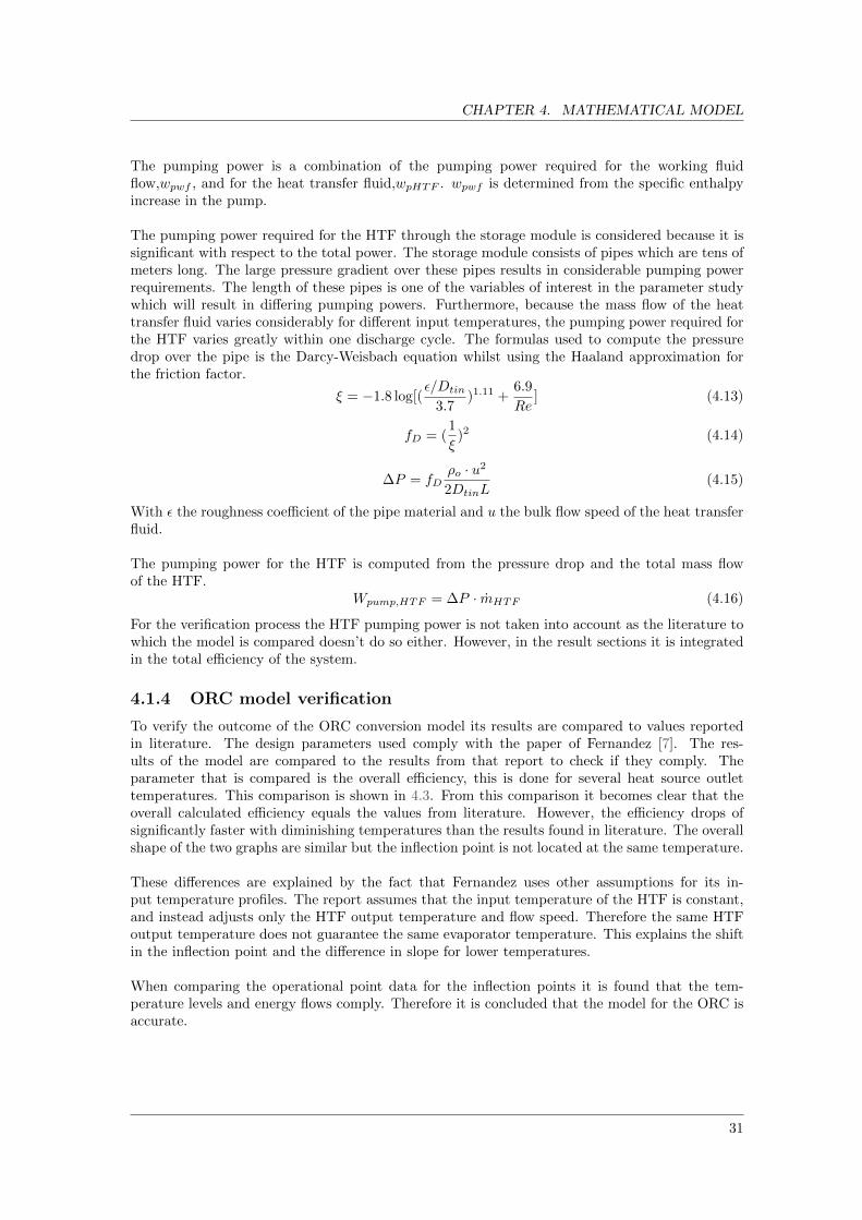
CHAPTER 4. MATHEMATICAL MODEL
The pumping power is a combination of the pumping power required for the working fluidflow,wpwf , and for the heat transfer fluid,wpHTF . wpwf is determined from the specific enthalpyincrease in the pump.
The pumping power required for the HTF through the storage module is considered because it issignificant with respect to the total power. The storage module consists of pipes which are tens ofmeters long. The large pressure gradient over these pipes results in considerable pumping powerrequirements. The length of these pipes is one of the variables of interest in the parameter studywhich will result in differing pumping powers. Furthermore, because the mass flow of the heattransfer fluid varies considerably for different input temperatures, the pumping power required forthe HTF varies greatly within one discharge cycle. The formulas used to compute the pressuredrop over the pipe is the Darcy-Weisbach equation whilst using the Haaland approximation forthe friction factor.
ξ = −1.8 log[(ε/Dtin
3.7)1.11 +
6.9
Re] (4.13)
fD = (1
ξ)2 (4.14)
∆P = fDρo · u2
2DtinL(4.15)
With ε the roughness coefficient of the pipe material and u the bulk flow speed of the heat transferfluid.
The pumping power for the HTF is computed from the pressure drop and the total mass flowof the HTF.
Wpump,HTF = ∆P · mHTF (4.16)
For the verification process the HTF pumping power is not taken into account as the literature towhich the model is compared doesn’t do so either. However, in the result sections it is integratedin the total efficiency of the system.
4.1.4 ORC model verification
To verify the outcome of the ORC conversion model its results are compared to values reportedin literature. The design parameters used comply with the paper of Fernandez [7]. The res-ults of the model are compared to the results from that report to check if they comply. Theparameter that is compared is the overall efficiency, this is done for several heat source outlettemperatures. This comparison is shown in 4.3. From this comparison it becomes clear that theoverall calculated efficiency equals the values from literature. However, the efficiency drops ofsignificantly faster with diminishing temperatures than the results found in literature. The overallshape of the two graphs are similar but the inflection point is not located at the same temperature.
These differences are explained by the fact that Fernandez uses other assumptions for its in-put temperature profiles. The report assumes that the input temperature of the HTF is constant,and instead adjusts only the HTF output temperature and flow speed. Therefore the same HTFoutput temperature does not guarantee the same evaporator temperature. This explains the shiftin the inflection point and the difference in slope for lower temperatures.
When comparing the operational point data for the inflection points it is found that the tem-perature levels and energy flows comply. Therefore it is concluded that the model for the ORC isaccurate.
31
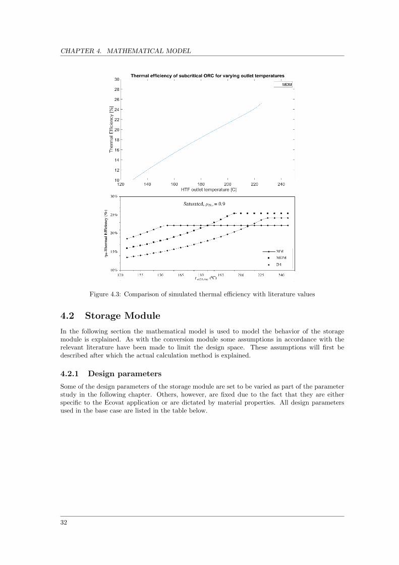
CHAPTER 4. MATHEMATICAL MODEL
Figure 4.3: Comparison of simulated thermal efficiency with literature values
4.2 Storage Module
In the following section the mathematical model is used to model the behavior of the storagemodule is explained. As with the conversion module some assumptions in accordance with therelevant literature have been made to limit the design space. These assumptions will first bedescribed after which the actual calculation method is explained.
4.2.1 Design parameters
Some of the design parameters of the storage module are set to be varied as part of the parameterstudy in the following chapter. Others, however, are fixed due to the fact that they are eitherspecific to the Ecovat application or are dictated by material properties. All design parametersused in the base case are listed in the table below.
32

CHAPTER 4. MATHEMATICAL MODEL
Variable Range/Value Motivation SourcesEe 7.48 · 103 [kWh] Required electricity storage capacity ApplicationPe 300 [kW] Required electrical power Application
Tcmax 643 [K] Limited to critical temperature working fluid MaterialTcmin 448 [K] Cutoff to ensure minimal efficiency ORC modelingCc 557 [K] Cutoff to not exceed critical temperature MaterialL 20 [m] Subject of parameter study -
dpipe 0.02 [m] Subject of parameter study -
Table 4.2: Boundary conditions for the storage module
4.2.2 Storage dimensions and segmentation
The overall storage size necessary is determined by the thermal storage capacity needed to achievethe goals of the system. The amount of thermal storage capacity is determined by the electricstorage capacity and the average conversion efficiency. The thermal power needed is determinedby the electric power and the minimal conversion efficiency. To limit the size of the storage modulea minimum conversion efficiency of 10% and an average conversion efficiency of 12% are assumed.
Eth =Eeηavg
(4.17)
Pth =Peηmin
(4.18)
How much concrete is needed to store this amount of energy is calculated as follows
mc =Eth
cc · (Tcmax − Tcmin)(4.19)
With cc being the specific heat capacity of concrete, and Tcmax and Tcmin the maximum andminimum concrete temperature respectively. The maximum concrete temperature is determinedby the maximum temperature allowed for the working fluid. The minimal concrete temperatureis determined by the lowest temperature for which a conversion efficiency of at least 10% can beachieved.
Once the total amount of storage material which is needed is known, the number of heat ex-changer pipes is determined. The preferred number of pipes is the minimum needed to ensure theneeded thermal power can be supplied at the lowest output temperature. To extract the neededthermal power a certain HTF mass flow is needed. To determine the total HTF mass flow anHTF temperature increase of 33 degrees is assumed inside the storage module. This is lowest thetemperature increase described by the ORC module over the entire relevant modeling range.
mHTF =Pth
cHTF · Tpinch(4.20)
The number of pipes used in the concrete is minimized whilst allowing for the needed thermalpower to be extracted. This is done by assuming an arbitrary starting number of pipes, npipes,calculating the overall heat transfer coefficient, determining the number of pipes needed with thisheat transfer coefficient, and using the resulting value as the starting point for the next iteration.
Firstly the flow speed of the HTF inside the pipe is determined. After this step the heat transfercoefficient, h, is calculated. This step is elaborated upon in the internal heat transfer section
mpipe =mHTF
npipes(4.21)
33

CHAPTER 4. MATHEMATICAL MODEL
uHTF =mpipe
ρHTF· 1
Apipe(4.22)
In which mpipe is the mass flow through one of the pipes. uHTF and ρHTF are the flowspeed ofthe HTF and Apipe the flow area of the pipe.
The volume of the concrete around the pipe is determined by dividing the total needed volume ofconcrete by the number of pipes. The outer radius of the concrete is calculated at a given pipelength, L. The length of the pipes can be varied but must fit inside the tank, for the calculationsa length of 20 meters was used.
Vc =mc
ρc(4.23)
Vpipe =Vc
npipes(4.24)
Rc =
√Vcπ ·N
+ r2t (4.25)
With Vc the total volume of the concrete, Vpipe the concrete volume per pipe and rc the radius ofthe concrete segment per pipe.
The heat transfer coefficient inside the pipe is used to arrive at an overall heat transfer coeffi-cient from the concrete to the HTF. This overall heat transfer coefficient is used to determine theminimum number of pipes needed to achieve the needed thermal power, for an assumed pinchtemperature of 10 degrees.
AU = L · h · π · dpipe (4.26)
npipes =Pth
AU · Tpinch(4.27)
This new number of pipes is used as input for the next iteration of the calculation. Once therounded value for the number of pipes needed to achieve the thermal power is stable, the iterativefunction is halted and the final value for the number of pipes is used in further calculations.
4.2.3 Internal heat transfer
The temperature and flow speed of the HTF varies continuously during the charge and dischargephases. Therefore, the heat transfer rate also varies and is reevaluated every time step, for eachlocation. This is done by subsequent calculation of the flow speed, Reynolds number, Nusseltnumber and finally the heat transfer coefficient. The equations used for these calculations arelisted below. Due to the pipes being very long in comparison to their diameter the flow is assumedto be fully developed and the fully developed regime is used for the entire pipe length.
The heat transfer coefficient is used to determine the thermal power flowing from the concreteinto the HTF. The thermal power per unit length for each time interval and position along thepipe is calculated as follows
Pth(i, j) = h(i, j) ·Dpipe · π ·∆z · (THTF (i, j)− Tc(i, j, 1)) (4.28)
How he temperature of the concrete, Tc, used in this equation is determined, is discussed in thenext section.
4.3 Concrete conduction model
To determine the charging and discharging behavior of the concrete storage module, the rect-angular concrete block is subdivided into smaller cylindrical segments. Each cylindrical segment
34

CHAPTER 4. MATHEMATICAL MODEL
corresponds to the concrete surrounding one of the heat exchanger pipes. The cylindrical geometryfor the segments is used because of symmetry and modeling simplicity considerations. The radiusof the cylinders is adjusted so that the total volume of the concrete is not altered. A schematicrepresentation of how these cylinders are arranged within the rectangular concrete is shown infigure 4.4. The indicated diameters dtube and d are equal to 2Rtube and 2R respectively.
Figure 4.4: Schematic representation of some cylindrical segments inside the bulk concrete
A simplified version of the heat equation is used in conjunction with the finite difference methodto develop a mathematical model for the temperature gradient inside the cylinders. To do this,firstly the governing equations and boundary conditions are determined and the discretization isdiscussed. Secondly the discretization is applied to the equations to arrive at a finite differencemodel of the storage module. The following section elaborates upon these steps and discusses howthese are implemented.
4.3.1 Governing Equations and Boundary Conditions
To simplify the mathematical model a number of assumptions are made about the storage moduleand its behavior. These assumptions, along with the simplified version of the heat equation, arelisted below.
1. The heat transfer through the segment is assumed to be rotationally symmetrical2. The perimeter of the concrete section is perfectly insulated allowing heat to be added or ex-tracted through the central tube only3. The flow of the heat transfer fluid is fully developed and uniform in the entire pipe4. The thermal resistance of the tube is negligible
ρC∂T
∂t= −k(
∂2T
∂r2+
1
r
∂T
∂r+∂2T
∂z2) (4.29)
This equation holds for the domain Ω = (z, r) ∈ R|0 < z < L,Rtube < r < R. On the boundary Γof the domain Ω the following boundary conditions are applied.
∂T
∂r(z,R) = 0, 0 ≤ z ≤ L
35

CHAPTER 4. MATHEMATICAL MODEL
∂T
∂z(0, r) =
∂T
∂z(L, r) = 0, Rtube ≤ r ≤ R
−k∂T∂r
(z,Rtube) = h(T − T∞), 0 ≤ z ≤ L
In this equation T∞ refers to temperature of the heat transfer fluid flowing through the pipe.
These boundary conditions correspond with an adiabatic outer layer of the cylinder, and con-vectional heat transfer between the concrete and the heat transfer fluid.
4.3.2 Discretization
A schematic representations of the modeled domain is shown in figure 4.5. During discretizationthe temperature at specific locations inside the concrete are used to determine temperature of theentire segment. These locations are referred to as nodes and are represented by the black dots infigure 4.5. The positions of the nodes and the inter nodal distances are defined as.
zj = j∆z, j = 1(1)N,∆z =L
N − 1
rk = k∆r +Rtube, k = 1(1)M,∆r =(R−Rtube)M − 1
ti = i∆t, i = 1(1)O,∆t =ttotalO − 1
The final expression defines the time discretization with a total simulated time ttotal and a timestep size of ∆t.
The partial differential equation is integrated over time and applied to all the nodes, howeverthe differential terms are replaced by their finite difference approximations. The finite differenceapproximations are defined using the central difference method and are listed below.
∂T
∂t|i, j, k =
T i+1j,k − T ij,k
∆t(4.30)
∂2T
∂r2|j,k =
Tj,k+1 − 2Tj,k + Tj,k−1
∆r2(4.31)
∂T
∂r|j,k =
Tj,k+1 − Tj,k−1
2∆r(4.32)
∂2T
∂z2|j,k =
Tj+1,k − 2Tj,k + Tj−1,k
∆z2(4.33)
Furthermore, to enable multiple finite difference methods the variable θ is introduced. θ can
assume the values of 1, 0 and1
2to utilize the Euler implicit, Euler explicit or Crank-Nicholson
method respectively. The general discretized version of the differential equation with inclusion ofthe variable θ is
τ i =T ij,k+1 − 2T ij,k + T ij,k−1
∆r2+T ij,k+1 − T ij,k−1
2∆r+T ij+1,k − 2T ij,k + T ij−1,k
∆z2(4.34)
T i+1j,k − T ij,k
∆t= (1− θ) · τ i + θ · τ i+1 (4.35)
36

CHAPTER 4. MATHEMATICAL MODEL
Figure 4.5: Schematic representation of concrete discretization
The fully discretized and integrated function using the Euler Implicit method is therefore as follows
T ij,k = T i+1j,k + α∆t(
T i+1j,k+1 − 2T i+1
j,k + T i+1j,k−1
∆r2+
1
Rk
T i+1j,k+1 − T
i+1j,k−1
2∆r+T i+1j+1,k − 2T i+1
j,k + T i+1j−1,k
∆z2)
(4.36)
These approximations are abbreviated versions of the Taylor series expansions for first and secondorder derivatives. The omission of the higher order terms of the series results in a truncation error.However, because the size of the error scales with higher orders of ∆r and ∆z the error remainsacceptable given sufficiently small values for ∆r and ∆z.
When these discretization methods are applied to the boundary Γ some adjustments needs tobe made. To illustrate this consider the nodes Tj,M . To perform the central difference methodapproximation the nodes Tj,M−1 and Tj,M+1 need to be known , but the nodes Tj,M+1 are notdefined and are considered ’ghost nodes’.
However, the boundary condition∂T
∂r(R, z) = 0, 0 ≤ z ≤ L states after discretization that
Tj,M+1 − Tj,M−1
2∆r= 0 (4.37)
This implies that Tj,M+1 = Tj,M−1 which is used in the approximations of the second order termsof the PDE. The same procedure can be used for the other adiabatic sections of Γ.
In the section of Γ where the boundary condition is convective the ghost node approach is also
37
CHAPTER 4. MATHEMATICAL MODEL
applied. The boundary condition in this region is
k∂T
∂r(Rtube, z) = h(T − T∞), 0 ≤ z ≤ L (4.38)
After discretization the following expression is found for the nodes in the region Tj,1.
kTj,2 − Tj,0
2∆r= h(Tj,1 − T∞) (4.39)
after rearranging the following expression is found for the ghost nodes Tk,0.
Tj,0 = Tj,2 −2h∆r
k(Tj,1 − T∞) (4.40)
These boundary conditions result in the following Euler implicit function for the nodes adjacentto the heat exchanger pipe.
T ij,1 = T i+1j,1 +α∆t(
2T i+1j,2 − 2T i+1
j,1 −2h∆r
k(T i+1j,1 − T i+1
∞ )
∆r2+
1
R1
h
k(T i+1j,1 −T
i+1∞ )+
T i+1j+1,1 − 2T i+1
j,1 + T i+1j−1,1
∆z2)
(4.41)Because the Euler implicit and Crank-Nicholson discretization schemes are used the system ofequations and boundary conditions is solved using the linear solver of Matlab. How the equationsare implemented in Matlab to achieve this is discussed in the next section.
4.3.3 Solving the system of equations
The linear solve function of Matlab can be used to solve systems of linear equations. The way itoperates is that when given the equation, Ab = c + d and matrix and vector A and c are known,the function will return the vector b.
For the purposes of this report the matrix and vectors need to be constructed in such a waythat they allow for a two dimensional problem, which can be solved both explicitly as implicitly.Firstly, the vector b is arranged for a two dimensional problem. The nodes are arranged by row,after all the nodes of the first row the first node of the second row starts until the entire grid isentered.
b = (T i+11,1 , · · ·, T
i+11,M , · · ·, T
i+1N,1 , · · ·, T
i+1N,M )T (4.42)
The matrix A is a M · N ×M · N matrix which contains the coefficients of the partial differen-tial equation for which the vector b is either the input and/or output (depending on the chosenmethod). The matrix is structured as a tridiagonal matrix with additional non zero diagonals onthe (M + 1) and the −(M + 1) diagonal to incorporate the coefficients for the axial dimension.The boundary conditions cause the first and last terms of the three main diagonals to differ fromthe rest, as well as the first M or last M terms of the (M+1) and −(M+1) diagonals respectively.A short overview of how the matrix is constructed is given below, as well as an overview of thevector c. For brevity some of the coefficients are combined into constants.
β = 2α∆t
(∆r)2(4.43)
γ = β(1 +h
k∆r − α∆th
kR+ 2
(∆r)2
(∆z)2) (4.44)
38

CHAPTER 4. MATHEMATICAL MODEL
ζ = β(∆r)2 + (∆z)2
(∆z)2(4.45)
µ =α∆t
r(k, j)2∆r(4.46)
A =
1 + θγ −θβ−θβ + µ 1 + θζ −θβ − µ
· · ·· · ·
−θβ + µ 1 + θζ −θβ − µ−2θβ 1 + θζ
(4.47)
D =
−θ α∆t(∆z)2
−θ α∆t(∆z)2
··−θ α∆t
(∆z)2
−θ α∆t(∆z)2
(4.48)
A =
A 2DD A D
· · ·D A D
2D A
(4.49)
d = Toij [β(h
k∆r − α∆th
kR), 0, · · ·, 0] (4.50)
39

CHAPTER 4. MATHEMATICAL MODEL
c = (4.51)
(1− (1− θ)γ)T i1,1 + 2(1− θ)βT i1,2 + 2(1− θ) α∆t(∆z)2T
i2,1 + T iHTF,1[β(
h
k∆r − α∆th
kR)]
((1− θ)β − µ)T i1,1 + (1− (1− θ)ζ)T i1,2 + ((1− θ)β + µ)T i1,3 + 2(1− θ) α∆t(∆z)2T
i2,2
.
.((1− θ)β − µ)T i1,M−2 + (1− (1− θ)ζ)T i1,M−1 + ((1− θ)β + µ)T i1,M + 2(1− θ) α∆t
(∆z)2Ti2,M−1
2(1− θ)βT i1,M−1 + (1− (1− θ)ζ)T i1,M + 2(1− θ) α∆t(∆z)2T
i2,M
(1− θ) α∆t(∆z)2T
i1,1 + (1− (1− θ)γ)T i2,1 + 2(1− θ)βT i2,2 + (1− θ) α∆t
(∆z)2Ti3,1 + T iHTF,2[β(
h
k∆r − α∆th
kR)]
(1− θ) α∆t(∆z)2T
i1,2 + ((1− θ)β − µ)T i2,1 + (1− (1− θ)ζ)T i2,2 + ((1− θ)β + µ)T i2,3 + (1− θ) α∆t
(∆z)2Ti3,2
.
.(1− θ) α∆t
(∆z)2Ti1,M−1 + ((1− θ)β − µ)T i2,M−2 + (1− (1− θ)ζ)T i2,M−1 + ((1− θ)β + µ)T i2,M + (1− θ) α∆t
(∆z)2Ti3,M−1
(1− θ) α∆t(∆z)2T
i1,M + 2(1− θ)βT i2,M−1 + (1− (1− θ)ζ)T i2,M + (1− θ) α∆t
(∆z)2Ti3,M
2(1− θ) α∆t(∆z)2T
iN−1,1 + (1− (1− θ)γ)T iN,1 + 2(1− θ)βT iN,2 + T iHTF,N [β(
h
k∆r − α∆th
kR)]
2(1− θ) α∆t(∆z)2T
iN−1,2 + ((1− θ)β − µ)T iN,1 + (1− (1− θ)ζ)T iN,2 + ((1− θ)β + µ)T iN,3
.
.2(1− θ) α∆t
(∆z)2TiN−1,M−1 + ((1− θ)β − µ)T iN,M−2 + (1− (1− θ)ζ)T iN,M−1 + ((1− θ)β + µ)T iN,M
2(1− θ) α∆t(∆z)2T
iN−1,M−1 + 2((1− θ)β − µ)T iN,M−1 + (1− (1− θ)ζ)T iN,M
The order of the nodes in vector c is the same as that used in b. However, to solve (semi)explicit systems the expression representing those nodes needs to contain the discretized form ofthe PDE including the boundary conditions. The resulting vector c has terms, when expressed insymbolic form are quite long and cluttered. This is due to the two dimensional approach, combinedwith the fact that implicit as well as explicit solution schemes need to be accommodated.
4.3.4 Verification
To verify the finite difference method described in the previous section, it is compared with ana-lytical solutions. The main objective of this step is to determine what the minimum amount ofnodes in each direction is that is needed to achieve accurate results.
The first analytical solution which is used is that of a semi infinite solid which is subjected toa convective heat transfer at its boundary. This first step in the verification procedure is meantto verify the results in the radial direction only. Therefore variations in the axial direction are nottaken into account. The analytical solution for the temperature distribution in such a solid is.
Tcx,t − TiT∞ − Ti
= erfc(x
2√αt
)− exp(hxk
+h2αt
k2)erfc(
x
2√αt
+h√αt
k) (4.52)
This solution only holds for a semi infinite solid in Cartesian coordinates. Therefore, the radialfinite difference solution needs to be altered to resemble its form in a Cartesian coordinate system,before the solutions can be accurately compared. This is done by drastically increasing the innertube diameter Rtube. By doing this the radius of the concrete becomes negligible in comparison
40
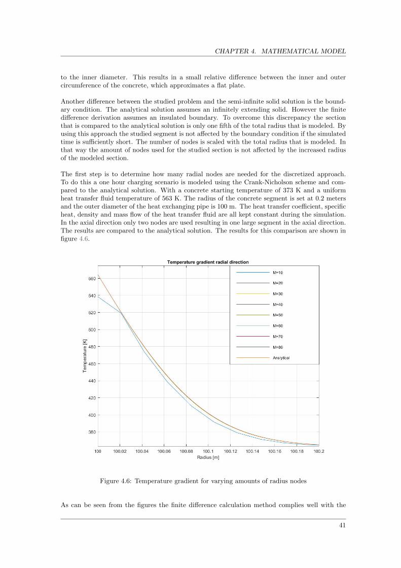
CHAPTER 4. MATHEMATICAL MODEL
to the inner diameter. This results in a small relative difference between the inner and outercircumference of the concrete, which approximates a flat plate.
Another difference between the studied problem and the semi-infinite solid solution is the bound-ary condition. The analytical solution assumes an infinitely extending solid. However the finitedifference derivation assumes an insulated boundary. To overcome this discrepancy the sectionthat is compared to the analytical solution is only one fifth of the total radius that is modeled. Byusing this approach the studied segment is not affected by the boundary condition if the simulatedtime is sufficiently short. The number of nodes is scaled with the total radius that is modeled. Inthat way the amount of nodes used for the studied section is not affected by the increased radiusof the modeled section.
The first step is to determine how many radial nodes are needed for the discretized approach.To do this a one hour charging scenario is modeled using the Crank-Nicholson scheme and com-pared to the analytical solution. With a concrete starting temperature of 373 K and a uniformheat transfer fluid temperature of 563 K. The radius of the concrete segment is set at 0.2 metersand the outer diameter of the heat exchanging pipe is 100 m. The heat transfer coefficient, specificheat, density and mass flow of the heat transfer fluid are all kept constant during the simulation.In the axial direction only two nodes are used resulting in one large segment in the axial direction.The results are compared to the analytical solution. The results for this comparison are shown infigure 4.6.
Figure 4.6: Temperature gradient for varying amounts of radius nodes
As can be seen from the figures the finite difference calculation method complies well with the
41

CHAPTER 4. MATHEMATICAL MODEL
analytical solution for all but the fewest amount of radial nodes. The system of equations wassolved using the the Crank-Nicholson scheme. The inaccurate results of the 10 node solution couldbe improved by using the Euler implicit scheme for the first radial node. However due to the over-all poor accuracy of this solution improving this solution was not pursued. To maintain accurate
results the timestep size dt equals the characteristic diffusion time tdif =dr2
α, with α being the
thermal diffusivity of the concrete. Because tdif is dependent on the number of radial nodes thetime steps varies for different node numbers. Good compliance with the analytical solution isobserved from 20 radial nodes onward. However, to obtain a more precise gage of the accuracy ofthe different solutions, a second test is performed.
The second test compares the energy increase of the concrete with the energy supplied to theconcrete by the heat transfer fluid. The energy absorbed by the concrete and the energy suppliedto the concrete are computed using the following formulas.
Etot =
M∑j=1
N∑k=1
Cj,k(TTimej,k − T 1j,k) (4.53)
Ein =
Time∑t=1
hA(T i1,1 − THTF )∆t (4.54)
ε =EtotEin
(4.55)
With Cj,k the thermal capacity of the segment and A the heat exchanging surface. For this testno segmentation is applied in the axial direction and the heat transfer fluid temperature To isassumed to be constant. ε indicates the degree to which the two solutions comply with a value of 1indicating total compliance. The results of this test are shown in table 4.3. These results indicate
M ε20 0.82130 0.93040 0.96350 0.97760 0.98470 0.98980 0.99190 0.993100 0.994
Table 4.3: Compliance between analytical and numerical solution for different radial node amounts
that the error between the two estimated values is less than 1% when 80 or more nodes are usedin the radial direction. Therefore this number of nodes is chosen as this amount of precision issufficient for the intended purpose. 4.7 shows the temperature evolution over time in the concretesegment during constant temperature charging.
The previous results have all assumed no axial segmentation and therefore a constant heat transferfluid temperature. To model the temperature change of the heat transfer fluid along the pipe lengththe following formula is used.
T iHTF,j+1 = T iHTF,j +hijA(T ij−1,1 − T iHTF,j−1)
mHTFCHTF(4.56)
T iHTF,j refers to the temperature of the heat transfer fluid at position j along the Z axis, m refersto the mass flow of the HTF along through the pipe.
42

CHAPTER 4. MATHEMATICAL MODEL
Figure 4.7: Time evolution of temperature gradient
N ε5 0.92210 0.95515 0.96420 0.96925 0.971
Table 4.4: Compliance to analytical solution of two dimensional simulation for varying axial nodeamounts
To determine how many axial nodes are needed to arrive at an accurate result, the same en-ergy balance technique is used as for the radial nodes. However, because the heat transfer fluidtemperature is not assumed to be constant anymore, the expression for Ein needs to be altered.The new expression uses the temperature difference between the fluid entering and exiting theheat transfer pipe,to determine the energy which is lost from the heat transfer fluid per time step.
Ein =
Time∑t=1
mCHTF (Toi1 − ToiN ·(M−1)+1)∆t (4.57)
A similar analysis is performed where the total added heat content of the concrete is comparedto the heat extracted from the heat transfer fluid. This comparison is performed whilst using 80radial nodes. The results are shown in table 4.4. The number of axial nodes has a large influenceon the total computational time needed to complete the simulation. Therefore a modest numberof 15 axial nodes is chosen for the simulation. 15 nodes allows for a reasonable simulation timewhilst providing reasonable accuracy.
43

CHAPTER 4. MATHEMATICAL MODEL
Figure 4.8: Temperature distribution in concrete segment during charging
With both radial and axial dependency incorporated 2-dimensional simulations are possible.Graphic representations of the temperature distribution inside a concrete segment after severalcharging times is shown in figure. These results correspond to 1, 12, 24 and 48 hours of chargingwith an input temperature of 573 K and a starting temperature of 363 K.
To arrive at a complete model of the system the output of the storage module is used as theinput for the ORC module, and vice versa. The results of the charging and discharging behaviorof this system are shown in the next chapter.
44

Chapter 5
Simulation Results
The model described in the previous chapter is used to model several charge and discharge scen-ario’s. These scenario’s are relevant for the application of the storage and conversion modules.Firstly the model for the ORC module is used to determine the appropriate operating range forefficient energy conversion. Secondly the base case system configuration mentioned in previouschapters is tested in two distinct scenario’s: constant power and user profile. The parameters ofthe base case are then altered to assess the impact of the parameters on the results for the differentscenario’s.
5.1 Operating range of the conversion module
The temperature range at which the ORC module can operate directly influences the size of thestorage module. Therefore it is desirable to have a large temperature range. However, the lowerand upper bounds of the temperature range are dictated by efficiency and material restrictions.The temperature range influences a number of aspects of the ORC, two of which will be discussedbelow. These are:
- Efficiency
- Turbine size
These parameters can have detrimental effects on the system costs and/or storage module per-formance when they exceed their respective operating ranges.
5.1.1 Efficiency
The efficiency of the conversion module is one of the main performance indicators of the system.Furthermore, a minimum value of 10 % is demanded during the full discharge cycle. The conversionefficiency of an ORC is predominantly determined by the inlet temperature of the HTF. Thereforethe inlet temperature has a lower limit which is allowed to ensure the minimum value. Theefficiency of the ORC module is modeled for a range of inlet temperatures, the results of whichare shown in figure5.1. As can be seen from the figure the minimal conversion efficiency of 10%cannot be guaranteed for inlet temperatures lower than 440 degrees centigrade. Therefore thistemperature is set as the temperature at which the storage module is considered fully discharged.
The upper temperature bound for the storage module is dictated by the material which is usedfor the HTF. The HTF used in the model is Therminol 66 which has a critical temperature of653 degrees Kelvin. To make sure the critical temperature of the HTF is not reached within thestorage module the upper limit for the storage temperature is set at 650 degrees K. This upper
45

CHAPTER 5. SIMULATION RESULTS
Figure 5.1: Thermal efficiency of sub-critical ORC for varying inlet temperatures
limit is within, but close to the maximum of, the allowable range for reinforced concrete.
5.1.2 Turbine Size
The component size of the different parts within the ORC module is not part of the scope of thisreport. However, the size of the turbine can influence the operating range of the entire system.This is because for certain working fluid and operating temperature combinations, the turbinewould have to be unfeasibly large to supply the needed power. In the report of Maraver anapproximation is put forth to estimate the size of a turbine, along with an acceptable range ofbetween 0.02 and 1 m. The size parameter of the turbine needed for the ORC used in this reportis 0.16 m and is therefore of no influence on the operating range.
5.2 Combined system
In this section the results of the charge and discharge simulations of the combined system arereported. Firstly, the charging and discharging behavior of the base case are considered. Secondly,the impact of the parameter alterations on the discharging behavior are studied. In figure 5.2 aschematic representation of the system is shown.
5.2.1 Initial setup
The initial setup refers to the setup discussed in the previous chapters. The parameters used inthis scenario are summarized in the table below. During discharge simulations a usage profiletaken from NEDU is used. NEDU is an organization which maps the electricity usage of Dutchhouseholds. The profile describes the energy usage during 2 consecutive winter days. The usedelectric power is scaled so that the total consumed energy matches the energy usage of 300 Dutchhouseholds in winter. A plot of the consumption curve is shown in figure 5.3. The results of thefull discharge simulation of the initial setup are shown in figures 5.4 and 5.5.
During discharge the conversion efficiency remained well above the dictated minimum of 10%.
46

CHAPTER 5. SIMULATION RESULTS
Figure 5.2: Schematic representation of ORC connected to the storage module
Figure 5.3: Consumption profile used in discharge simulations, created from data from [16]
However, the setup was not able to supply the required power for the full duration of the simu-lation, as the efficiency dropped drastically after the 42 hour mark. The simulation was abortedonce the efficiency dropped below the minimum value of 10%. The efficiency dropped due to a coldregion which had developed along the full length of the heat exchanger pipe. The temperaturedevelopment inside the storage module is visualized in figure 5.6. Note the cold region at thebottom right region of the final subplot, which corresponds to the exit of the heat exchanger pipe.Because the simulation was halted prematurely, the storage module still contains 17.62% of its
47
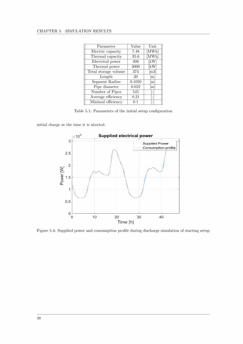
CHAPTER 5. SIMULATION RESULTS
Parameter Value UnitElectric capacity 7.48 [MWh]Thermal capacity 35.6 [MWh]Electrical power 300 [kW]Thermal power 3000 [kW]
Total storage volume 374 [m3]Length 20 [m]
Segment Radius 0.1050 [m]Pipe diameter 0.022 [m]
Number of Pipes 545 [-]Average efficiency 0.21 [-]Minimal efficiency 0.1 [-]
Table 5.1: Parameters of the initial setup configuration
initial charge at the time it is aborted.
Figure 5.4: Supplied power and consumption profile during discharge simulation of starting setup
48

CHAPTER 5. SIMULATION RESULTS
Figure 5.5: Thermal conversion efficiency of the ORC during discharge simulation
Figure 5.6: Concrete segment temperature development during discharge
49

CHAPTER 5. SIMULATION RESULTS
5.2.2 Base Case
Without altering the performance conditions of the system several options are possible to improvethe performance of the system. Two of these options are increasing either storage size or heatexchanger surface area. Due to cost considerations it was opted to increase the storage size of thesystem, as the storage material is cheaper than investing in more heat exchanging surface. Thetotal volume of concrete was increased by 20%, this configuration will for the rest of this chapter bereferred to as the base case. The parameters which have been updated are listed in the table below.
Parameter Value UnitElectric capacity 8.98 [MWh]Thermal capacity 42.72 [MWh]
Total storage volume 448 [m3]Segment diameter 0.115 [m]
Table 5.2: Parameter adjustments made to initial setup to arrive at the base case
The discharge experiment was repeated for the base case. The results of this simulation are shownin figures 5.7 and 5.8. The increased concrete volume allows the system to adhere to the desiredsupply curve for the full duration of the simulation. The average efficiency during the dischargeperiod is 21.15% and after 48 hours of discharge 16.4% of the initial charge remains. After thewindow of 48 hours the system was still able to keep discharging for an additional 9.5 hours. Atthe end of the full 57.5 hours of discharge the SOC was 3.62%.
The results of the full power discharge simulation of the base case are shown in figures 5.9 and 5.10.Due to the higher power the concrete region near the heat exchanger tube discharges quickly. Thisresults in a quickly dropping HTF temperature and conversion efficiency. The average efficiencyduring the discharge is but already dalls below the critical value of 10% after 17.55 hours. Afterthis time 22.82 % of the original charge still remained in the storage module.
50
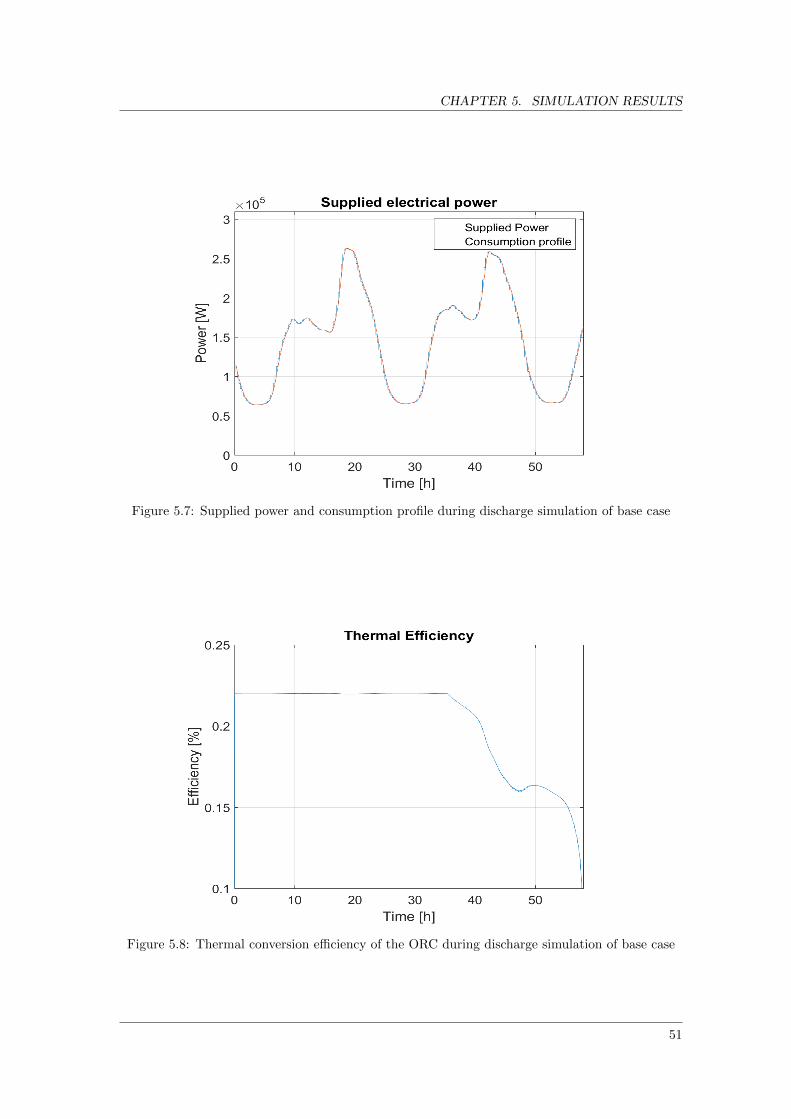
CHAPTER 5. SIMULATION RESULTS
Figure 5.7: Supplied power and consumption profile during discharge simulation of base case
Figure 5.8: Thermal conversion efficiency of the ORC during discharge simulation of base case
51

CHAPTER 5. SIMULATION RESULTS
Figure 5.9: Inlet and outlet temperature of the ORC for during full power discharge
Figure 5.10: Thermal conversion efficiency of the ORC during full power discharge
52

CHAPTER 5. SIMULATION RESULTS
5.2.3 Parameter study
To assess the impact of variations in the storage parameters on the discharge behavior a para-meter study is performed. The parameters that are altered are the length and the amount ofheat exchanger pipes. The total amount of storage material is kept constant during all simula-tions. Both the typical consumption profile and the full power discharge simulations are conducted.
The variables of interest are the same ones discussed in the previous section: discharge time,overall efficiency and the state of charge at the end of discharge. One variable that is added tothe analysis: the total meters of pipe needed for the configuration. The most costly component ofthe storage module is the heat exchanger and is therefore of interest. The results of the consumerprofile parameter study are summarized in the following table.
Consumption profileTime Efficiency SOC pipe m
Starting Setup 42.13 21.3 17.84 10900Base case 57.5 20.18 3.62 10900
Length +25% 56.87 20.09 3.95 10900Length -25% 57.5 20.23 3.09 10900Pipes +10% 57.5 20.23 3.23 12000Pipes -10% 57 20.04 3.72 9800Pipes -20% 44.14 21.38 26.57 8720
Table 5.3: Parameter study results for the consumption profile discharge regime
The results for the consumption profile parameter study do not vary greatly from case to case. Thelarge difference between the discharging time of the starting setup and the base case is caused bythe shape of the consumption profile. The large peak around the 43 hour mark puts a large strainon the system, causing the starting setup to fail around this point. However, once the simulationpasses this point the required power falls again. This allows configurations which reach this pointto continue for a considerable amount of time.
The ’Pipes -10%’ configuration is able to perform similarly to configurations with larger heatexchanger surfaces. However, further decreasing the amount of heat exchanger surface drasticallydiminishes the discharge time. This is caused by the phenomenon discussed in the previous para-graph.
Full powerTime Efficiency Pumping power [kW] npipes pipe m
Starting Setup 18.95 20.75 4.03 545 10900Base case 22.52 20.75 3.99 545 10900
Length +25% 21.42 20.87 5.86 436 10900Length -25% 23.53 20.56 2.45 727 10900Pipes +10% 23.52 20.72 3.59 600 12000Pipes -10% 21.32 20.77 4.61 490 9800
Table 5.4: Parameter study results for the full power discharge regime
The results of the full power discharge show that increased discharge times are achieved for the’Length + 25%’ and the ’Pipes +10%’ scenario’s. These scenario’s have a lower overall efficiencythan the base case. The inverse is true for the ’Length +25%’ and the ’Pipes -10%’ scenario’s.Which have shorter discharge times and longer overall efficiencies.
53

CHAPTER 5. SIMULATION RESULTS
The explanation for the discharge time differences is found in the pumping power needed forHTF circulation. The scenario’s which perform better with regard to the discharge time, bothhave an increased number of heat exchanger pipes. This results in a lower bulk velocity inside theheat exchanger tubes which greatly influences the needed pumping power. As the overall efficiencydrops, the mass flow rate and pressure drop over the storage module increase. The increase inpumping power that follows these changes lowers the overall efficiency until the minimum efficiencyof 10% is reached.
5.3 Economic performance
To assess the economic performance added by the electricity storage system, an analysis of theadded value of the system is performed. To perform this analysis assumptions need to be madeabout the value of the different energy streams. For the electricity and heat supplied by the sys-tem the average consumption prices of electricity and heat supplied by natural gas, 20 and 6.5eurocents per kWh respectively [14], are used. The energy used to charge the system is assumedto be costless. This assumption is justified due to the flexible charge capabilities of the systemand the expected rise in renewable energy sources.
The added value of a full storage discharge using the consumption profile and under full power isshown in the tables below. The total value is the value of both the thermal and electric energywhich was discharged. The added value is the value created by the electric energy. The valueand added value for all configurations in both discharge regimes is similar. Only deviating for theconfigurations where not all energy could be discharged. To place these results into context they
Consumption profileEtot [MWh] Eelec [MWh] Eth [MWh] Total Value [$] Added value [$]
Heat only 42.72 0 42.72 3168 0Base case 41.17 8.31 32.86 4348 1180
Length +25% 41.03 8.24 32.79 4327 1159Length -25% 41.40 8.36 33.04 4373 1205Pipes +10% 41.34 8.36 32.98 4369 1200Pipes -10% 41.13 8.24 32.89 4334 1166
Table 5.5: Supplied energy and its value during discharge under the consumption profile regime
Full powerEtot [MWh] Eelec [MWh] Eth [MWh] Total Value [$] Added value [$]
Heat only 42.72 0 42.72 3168 0Base case 42.62 8.84 33.77 4545 1378
Length +25% 42.60 8.89 33.71 4528 1384Length -25% 42.64 8.77 33.87 4528 1368Pipes +10% 42.63 8.83 33.80 4538 1378Pipes -10% 30.55 6.35 24.20 3254 93.8
Table 5.6: Supplied energy and its value during discharge under the full power regime
are compared to the system cost of the modeled system as well as its main alternative: Li-ionbatteries. The cost of the starting setup was already estimated in chapter 3 and resulted in anestimate of 820.000 USD. For the 20% concrete volume increase these costs only increase slightly
54

CHAPTER 5. SIMULATION RESULTS
to 830.000 USD. The cost per kWh installed of stationary Li-ion systems differs depending on theenergy to power ratio. A typical ratio for such systems is 5:1 which results in an average price ofapproximately 500 USD/kWh [1].
Total costs [$] Value per cycle [$] Added value [$] CyclesBase case 830000 4538.66 1370.4 605.66
Capacity matched 4420000 1931.54 1275.94 3464.12Power matched 750000 327.75 216.51 3464.12
Table 5.7: Total costs of electricity storage systems along with the value per cycle and the numberof cycles needed to offset the costs
The value per cycle refers to the value of the energy sold during the discharge. When the energysold during the discharge was charged in the normal Ecovat system and supplied as heat thiswould have created value as well. The added value is the difference between the revenue withand without the electricity storage module. In the final column the number of discharge cyclesneeded to offset the costs of the electricity storage is listed. It should be noted that the chargeand discharge cycles for the Li-Ion systems are considerably shorter than those of the proposedsystem. The proposed system takes 143 hours to fully charge, or 24 hours to match the storagecapacity of the smaller Li-ion system. In contrast the Li-ion systems only takes 5 hours to fullycharge.
In the previous analyses it was assumed that the energy to charge the system was procuredat no cost. This resulted in a net margin per kWh equal to the selling price per kWh for elec-tricity or heat. In the event that the electricity needs to be bought at higher prices the profitmargin shrinks. Because the profit margin for heat energy is smaller than for electricity, systemthat derive their value from heat energy are more sensitive to rises in the procurement price. Thiseffect is illustrated in figure 5.11 where the number of cycles needed to arrive at the break evenpoint is compared for several conversion efficiencies. Due to its low conversion efficiency the basecase is vulnerable to rises in procurement price.
Figure 5.11: Sensitivity of the number of cycles needed to break even to fluctuations in energyprocurement costs
55

Chapter 6
Conclusions
The conclusions of this report are separated into three different sections. The general storagemodule design, thermodynamic performance of the system and economic performance of the sys-tem. After these sections have been addressed recommendations are made for implementation inthe Ecovat system and interesting area’s for further study.
6.1 General module design
The main performance characteristics of the entire system were profitability and round trip effi-ciency.
To achieve a profitable system the system needs to be able to perform multiple services for itsconsumers. The service which aligns best with the current mode of operation of the Ecovat isthat of emergency power storage for its connected consumers. The parameters needed for sucha system are similar to that of congestion management on the distribution grid. Therefore thesetwo services are selected as the two services to be provided by the system.
The conversion efficiency of the storage module is determined by the used heat engine and thetemperature of storage. Of the studied heat engines the Stirling engine has the highest conversionefficiency at moderate temperatures, followed by the ORC and the steam cycle. However, Stirlingengines are not widely used in industry, especially for applications exceeding 25 kW. This practicalconsideration leads to the selection of the ORC as the preferred conversion method. The efficiencyreached by ORC’s is dependent on the used working fluid and system design. For the simulationa working fluid with a high critical temperature is preferred to allow high inlet temperatures. Arecuperator is adopted into the ORC design to increase the temperature of the waste heat stream.
The storage material which results in the lowest costs of the storage module is reinforced con-crete. The abundant availability and easy of use of concrete are additional advantages to usingconcrete. Because concrete is a solid with limited conduction capabilities more heat exchangingsurface is needed to supply the desired power.
The final system is designed to supply 300 kW of electric power and has a storage capacityof 35.6 MWh thermal, at a temperature drop of 195 degrees. The total concrete volume is 374cubic meters in which the heat exchanger consisting of 545, 20 m long, 2.2 cm diameter steel pipesare equidistantly integrated. The investment cost estimate of the storage and conversion moduleis 830.000 USD. The majority of the costs, 600.000 USD, is attributed to the conversion module.This holds true regardless of the heat engine used for the conversion module.
56

CHAPTER 6. CONCLUSIONS
6.2 Thermodynamic performance
During consumption profile discharge relatively small changes in storage capacity can greatly in-fluence the discharge time. Increasing the amount of storage material by 20% allows the system tooperate for 57.5 hours instead of 42 hours, a 36% percent increase. The fluctuating power demandsof the consumption profile influence the HTF mass flow rate and inlet temperature considerably.This has a large impact on the conversion efficiency, possibly lowering it below the minimum of10%.
The dimensional variations indicate that during consumption profile discharge, configurations thatlimit the flow speed through the heat exchanger perform better. The configurations with shorterand/or more heat exchanger pipes have longer discharge times and higher efficiencies. How muchthese parameters influence the discharge time does depend greatly on the shape of the dischargeprofile.
During full power discharge the configurations with limited mass flow rate allow for the longestdischarge time. This is mainly caused by the low average pumping power during the dischargecycle.
6.3 Economic performance
Overall the high temperature heat storage module with ORC conversion module provides themost cost effective way to store large quantities of energy. When compared to the most prolificelectricity storage technique, Li-ion, the discussed system is the cheaper option by a factor of 5.When compared to the power matched design the installation costs of both the systems are similar.
The number of discharge cycles for the system to break even is 606 as compared to 3465 forthe Li-ion systems. So when providing backup power for contracted suppliers the proposed systemwould reach profitability earlier than comparable Li-ion systems.
Due to the lower conversion efficiency of the proposed HTS system more PTU’s are needed tocharge the system than comparable Li-ion systems. This increases the likelihood of not being ableto charge at reduced costs.
Systems which derive their value from both heat and electricity are more vulnerable to procure-ment price fluctuations. The per kWh value of heat is lower and therefore increases in procurementprice have a large impact on the profit margin and number of cycles needed to break even.
The added value of all electricity storage systems is derived from the difference between the priceof electricity and that of heat. Therefore the profitability of the systems is vulnerable to relativeprice increases of heat compared to electricity.
6.4 Recommendations
6.4.1 Application
Due to the low costs per kWh storage capacity the service of providing backup power can beprovided most cost effectively using the HTS setup. Whether the system will prove to be prof-itable, is however highly dependent on the value which will be attributed to this service. To
57
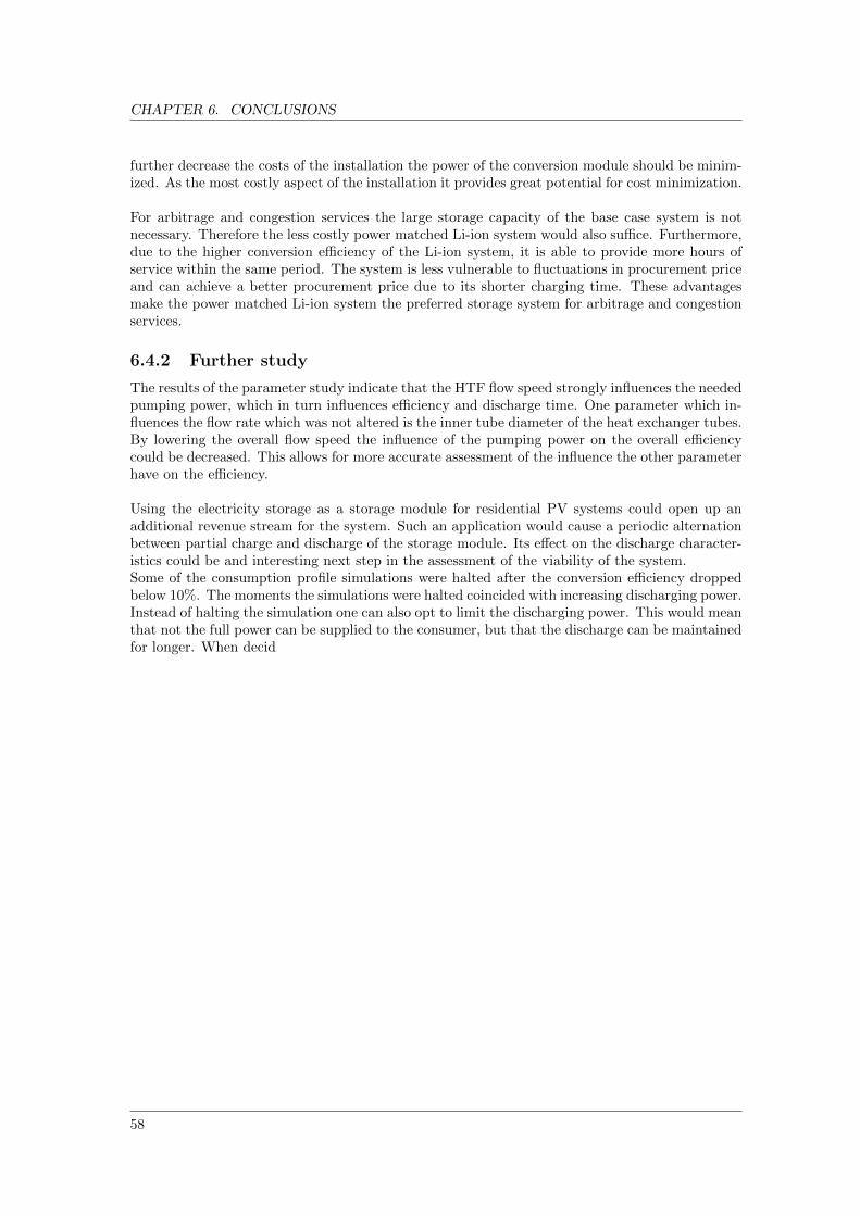
CHAPTER 6. CONCLUSIONS
further decrease the costs of the installation the power of the conversion module should be minim-ized. As the most costly aspect of the installation it provides great potential for cost minimization.
For arbitrage and congestion services the large storage capacity of the base case system is notnecessary. Therefore the less costly power matched Li-ion system would also suffice. Furthermore,due to the higher conversion efficiency of the Li-ion system, it is able to provide more hours ofservice within the same period. The system is less vulnerable to fluctuations in procurement priceand can achieve a better procurement price due to its shorter charging time. These advantagesmake the power matched Li-ion system the preferred storage system for arbitrage and congestionservices.
6.4.2 Further study
The results of the parameter study indicate that the HTF flow speed strongly influences the neededpumping power, which in turn influences efficiency and discharge time. One parameter which in-fluences the flow rate which was not altered is the inner tube diameter of the heat exchanger tubes.By lowering the overall flow speed the influence of the pumping power on the overall efficiencycould be decreased. This allows for more accurate assessment of the influence the other parameterhave on the efficiency.
Using the electricity storage as a storage module for residential PV systems could open up anadditional revenue stream for the system. Such an application would cause a periodic alternationbetween partial charge and discharge of the storage module. Its effect on the discharge character-istics could be and interesting next step in the assessment of the viability of the system.Some of the consumption profile simulations were halted after the conversion efficiency droppedbelow 10%. The moments the simulations were halted coincided with increasing discharging power.Instead of halting the simulation one can also opt to limit the discharging power. This would meanthat not the full power can be supplied to the consumer, but that the discharge can be maintainedfor longer. When decid
58

Bibliography
[1] International Renewable Energy Agency. Electricity storage and renewables: Costs and mar-kets to 2030. 55
[2] Ian H. Bell, Jorrit Wronski, Sylvain Quoilin, and Vincent Lemort. Pure and pseudo-purefluid thermophysical property evaluation and the open-source thermophysical property librarycoolprop. Industrial & Engineering Chemistry Research, 53(6):2498–2508, 2014. 28
[3] Nils Breidenbach, Claudia Martin, Henning Jockenhofer, and Thomas Bauer. Thermal EnergyStorage in Molten Salts: Overview of Novel Concepts and the DLR Test Facility TESIS.Energy Procedia, 99(March):120–129, 2016. 15
[4] Topsector Energie. Routekaart Energieopslag. 2015. v, v, v, v, 8, 9, 10, 12
[5] EPRI. Electric Energy Storage Technology Options: A White Paper Primer on Applications,Costs and Benefits. Epri, pages 1–170, 2010. v, 4
[6] European Commission. Roadmap 2050. Technical Report April, European Commision, 2012.1
[7] F. J. Fernandez, M. M. Prieto, and I. Suarez. Thermodynamic analysis of high-temperatureregenerative organic Rankine cycles using siloxanes as working fluids. Energy, 36(8):5239–5249, 2011. v, 25, 26, 31
[8] Antoni Gil, Marc Medrano, Ingrid Martorell, Ana Lazaro, Pablo Dolado, Belen Zalba, andLuisa F. Cabeza. State of the art on high temperature thermal energy storage for powergeneration. Part 1-Concepts, materials and modellization. Renewable and Sustainable EnergyReviews, 14(1):31–55, 2010. v, 14, 22
[9] Florian Heberle and Dieter Bruggemann. Exergy based fluid selection for a geothermal Or-ganic Rankine Cycle for combined heat and power generation. Applied Thermal Engineering,30(11-12):1326–1332, 2010. 25
[10] Elke Klaassen, Elke Klaassen, and Jasper Frunt. Assessing the impact of distributed en-ergy resources on LV grids using practical measurements ASSESSING THE IMPACT OFDISTRIBUTED ENERGY RESOURCES ON LV GRIDS. (October), 2015. 17
[11] Xing Luo, Jihong Wang, Mark Dooner, and Jonathan Clarke. Overview of current develop-ment in electrical energy storage technologies and the application potential in power systemoperation. Applied Energy, 137:511–536, 2015. v, 4, 7, 13
[12] Daniel Maraver, Javier Royo, Vincent Lemort, and Sylvain Quoilin. Systematic optimiza-tion of subcritical and transcritical organic Rankine cycles (ORCs) constrained by technicalparameters in multiple applications. Applied Energy, 117:11–29, 2014. 25, 26, 27
[13] Marc Medrano, Antoni Gil, Ingrid Martorell, Xavi Potau, and Luisa F. Cabeza. State of theart on high-temperature thermal energy storage for power generation. Part 2-Case studies.Renewable and Sustainable Energy Reviews, 14(1):56–72, 2010. 14
59

BIBLIOGRAPHY
[14] Milieucentraal. Energieprijzen. 54
[15] Riccardo Moro, Piero Pinamonti, and Mauro Reini. ORC technology for waste-wood to energyconversion in the furniture manufacturing industry. Thermal Science, 12(4):61–73, 2008. 25
[16] NEDU. Verbruiksprofielen electriciteit. v, 47
[17] Markus Preißinger and Dieter Bruggemann. Thermoeconomic Evaluation of Modular OrganicRankine Cycles for Waste Heat Recovery over a Broad Range of Heat Source Temperaturesand Capacities. Energies, 10(3):269, 2017. 25
[18] Sylvain Quoilin, Martijn Van Den Broek, Sebastien Declaye, Pierre Dewallef, and VincentLemort. Techno-economic survey of organic rankine cycle (ORC) systems. Renewable andSustainable Energy Reviews, 22:168–186, 2013. v, 21
[19] Siemens Brochure. Siemens Organic Rankine Cycle Waste Heat Recovery with ORC. pages0–25, 2014. 25
[20] E. H. Wang, H. G. Zhang, B. Y. Fan, M. G. Ouyang, Y. Zhao, and Q. H. Mu. Studyof working fluid selection of organic Rankine cycle (ORC) for engine waste heat recovery.Energy, 36(5):3406–3418, 2011. 25
[21] World Energy Council (WEC). World Energy Resources. page 1028, 2016. v, 5
[22] Chi-jen Yang. Chapter 2 - Pumped Hydroelectric Storage. Elsevier Inc., 2016. 6
60