the possible influence of urban surfaces on rainfall ...directory.umm.ac.id/data...

Ž .Atmospheric Research 54 2000 15–39www.elsevier.comrlocateratmos

The possible influence of urban surfaces on rainfalldevelopment: a sensitivity study in 2D in the

meso-g-scale

J. Thielen c,), W. Wobrock b, A. Gadian c, P.G. Mestayer a,J.-D. Creutin d

a ( )ECN DMEE , SUBMESO-GdR CNRS 1102, Nantes, Franceb LaMP, UniÕersite Blaise Pascal, Clermont-Ferrand, France´

c Department of Applied Physics, UMIST, Manchester, UKd LTHE, Grenoble, France

Received 14 December 1998; received in revised form 7 December 1999; accepted 17 February 2000

Abstract

Urban areas can represent a considerable part of the model domain in meso-scale numericalsimulations with typical horizontal domain lengths of 20–200 km. This paper addresses thequestion of the extent of the influence of urban surfaces on the development of convectiveprecipitation in meso-g-scale numerical models. For this purpose, a spatially variable parameteri-zation scheme for surface sensible heat flux, surface latent heat flux, and roughness is introducedinto a meso-scale numerical model. A sensitivity study in 2D is performed to assess the impact ofvariations of the individual parameters on the development of precipitation. The results indicatethat surface conditions should not be neglected and can have considerable influence on convectiverainfall. It appears that within a time frame of 4 h it is particularly the sensible heat flux variationsthat have the most significant impact. q 2000 Elsevier Science B.V. All rights reserved.

Keywords: Urban meteorology; Meso-scale meteorological modelling; Interface soil–atmosphere

1. Introduction

Urban areas modify boundary layer processes mostly through the production of anŽurban heat island Vukovich and Dunn, 1978; Bornstein, 1986; Draxler, 1986; Oke,

) Corresponding author. Department of Applied Physics, UMIST, P.O. Box 88, Manchester M60 1QD, UK.Ž .E-mail address: [email protected] J. Thielen .

0169-8095r00r$ - see front matter q 2000 Elsevier Science B.V. All rights reserved.Ž .PII: S0169-8095 00 00041-7

( )J. Thielen et al.rAtmospheric Research 54 2000 15–3916

. Ž1987 and by increasing turbulence through locally enhanced roughness Loose and.Bornstein, 1977; Stull, 1988; Theurer et al., 1992; Rotach, 1993a,b . Thus, as a

consequence, larger scale meteorological processes can also be affected by the presenceŽ .of urban agglomerations Huff, 1986; Oke, 1987; Goldreich, 1995 .

Although the importance of the lower boundary for meso-scale models has beenŽ .discussed for some time see e.g., Pielke, 1984; Pielke et al., 1991 , detailed representa-

tion of the surface heat and moisture fluxes has only recently been included inŽ .meso-scale numerical modelling Lee et al., 1993; Moussiopoulos, 1994 . The principal

reasons for this are that the heat and moisture transfers at the surface depend on aŽ .variety of soil parameters i.e., heat capacity, permeability, porosity as well as

Ž .vegetation parameters i.e., type of plant, leaf surface, root density , for which explicitdata are mostly not available. A realistic treatment of the lower boundary, however,requires these parameters for the calculation of the energy and moisture transport.

ŽExisting soil models are mostly designed and validated for rural surfaces e.g.,.Sievers et al., 1983; Noilhan and Planton, 1989; Lee et al., 1993; Braud et al., 1995 .

However, in meso-scale numerical models, with grid lengths of 100 m up to a fewkilometers, urban areas can represent a considerable fraction of the model domain and

Žshould not be neglected. In urban areas, artificial surfaces concrete, asphalt, stone. Ž .pavements, slate and natural surfaces parks, trees, gardens vary on a relatively small

spatial scale, which makes the definition of representative parameters for meso-scalegrid dimensions difficult. Further, the transfer coefficients for heat and momentum areaffected by turbulent flow, which is not well-established in inhomogeneous urbanenvironments.

The complexity of the system increases further when precipitation is considered. Inthe case of intensive rainfall, for example, impermeable and normally dry surfaces canbe transformed into temporary lakes, locally enhancing the evaporation. On the otherhand, drainage systems transport away much of the rainwater, which is then no longeravailable for evapo-transpiration processes. Thus, modifications of the precipitationfields due to the presence of urban areas are of particular interest for meteorologists, aswell as being crucially needed by hydrologists.

Ž .On the synoptic scale Loose and Bornstein 1977 have shown by observation andmodelling that urban areas may significantly affect synoptic scale fronts. In cases ofweak to moderately developed heat islands, most fronts slow down when moving overthe urban area. In cases of pronounced heat islands, the retardation is less pronouncedbut still observable.

Effects of large cities on meso-scale or convective rainfalls were studied by theŽ .Metropolitan Meteorological Experiment METROMEX , which took place in the 1970s

Ž .in the US Changnon et al., 1977; Huff, 1986 . The experiment suggested that largeurban areas could have an impact on the frequency of convective storms. Enhancementof rainfall frequencies over and downwind of urban areas was one of the results of thisvast study. In the vicinity of St. Louis, for example, heavy storm events occur twice asoften as in areas without urban agglomerations, and rain bearing cells exposed to theurban environment yield more precipitable water than comparable cells in rural areasŽ .Huff, 1977 . Rainfall enhancement is observed for the urban area itself and at a distanceof 40 km downwind of the city centre. This increase was attributed mostly to the

( )J. Thielen et al.rAtmospheric Research 54 2000 15–39 17

modifications of the airflow due to the heat island and the increased roughness. Thepossibility that the presence of increased giant CCN concentrations originating from theurban area could also play a role in the precipitation processes was not excluded.

The present study is a first step in the development of a surface model for both ruraland urban areas, in a meso-g-scale meteorological model. The sensitivity of meso-scaleprocesses to the lower boundary is assessed, using surface and soil-dependent parame-ters. Both rural and urban surfaces are considered, allowing on the one hand a study ofthe influence of urban areas on cloud and rainfall development, and on the other hand anassessment of the relative importance of the individual surface parameters. To achievethis, a three-parameter scheme describing surface roughness and soil-dependent surface

Žsensible and latent heat fluxes is introduced into the Clark model Clark, 1977; Clark.and Grabowski, 1991 , as described in Section 2.

Processes leading to precipitation are essentially 3D. Since it is difficult, however, tomake extensive sensitivity studies in a 3D framework, for this study the 2D version ofthe model is used. It is assumed that the 2D simplification provides a good means toassess the relative importance of the response of the atmosphere to different surfaceparameters that describe the surface conditions. Effects becoming apparent in 2D shouldalso be qualitatively relevant in 3D, even if quantitative differences should be expected.Those surface parameters affecting rainfall in the 2D simulations would then be tested ina 3D framework in further studies.

The set-up of the simulations is presented in Section 3. The impact of the individualsurface parameters on meso-scale processes is assessed by analysing the rainfall

Ž .development Section 4 . Conclusions are drawn in Section 5.

2. The Clark model

Ž .The Clark model e.g., Clark, 1977; Clark and Farley, 1984 represents a finite-dif-ference approximation to the anelastic, non-hydrostatic equations of motion. It expandsthe system variables around profiles of an idealized atmosphere with constant stabilityŽ . Ždenoted as overbar , deviations from the hydrostatic equilibrium denoted with a

. Ž .prime , and space- and time-dependent perturbations denoted as double prime . TheNavier–Stokes equation is approximated as:

ydz QY pX

Et i jY Yr sy2 rV=zy=p qkr g y q´ q yq yq yq qv C R Iž /d t g p ExQ j

1Ž .

where r is the density of air, z is the 3D wind vector, k is the unit vector in the verticaldirection, V is the angular rotation vector of the earth, p is the atmospheric pressure, gis the gravitational constant, Q is the potential temperature, ´ is R rR y1 with Rv d d

and R being the gas constants of dry and humid air, g is the ratio of the heat capacitiesvŽ .at constant pressure and constant volume c rc , q is the water vapour mixing ratio,p Õ v

q , q , and q are the mixing ratios of cloud water, rainwater and ice, respectively, andC R I

t is the stress tensor describing the subgrid-scale turbulent processes.i j


Heat and moisture development are expressed by)dQ rL

)r s C q=P rK =Q 2Ž .Ž .d Hd t c Tp

dqvr syrC q=P rK =q 3Ž .Ž .d H vd t

where L is the latent heat released from condensation processes, T is the temperature,C gives the rate of all phase transition of atmospheric water, and Q ) is a non-dimen-d

X Y) Ž .sional normalized potential temperature defined as Q s Q qQ rQ . The budget

equations of the mixing ratios of cloud water, q , rainwater, q , and ice, q , are givenC R IŽ .in detail in Bruintjes et al. 1994 . K is the Richardson number dependent variableH

Ž .eddy mixing coefficient used for heat and moisture transport Clark, 1979 .The microphysics in the model includes warm rain parameterization based on the

Ž .Kessler 1969 scheme, and ice parameterization based on the work of Koenig andŽ . ŽMurray 1976 . Since this model has been described elsewhere e.g., Clark, 1977; Clark

.and Farley, 1984 , only the basic features and modifications are described here.

2.1. The surface parameters

The parameters used to characterize the surface in this study act on the sensible andlatent heat fluxes as well as on the surface roughness. The surface forcing of the heatand moisture fluxes are described by adding the following terms to the subgrid-scale

)Ž . Ž .mixing terms rK EQ rEz and rK Eq rEz in Eqs. 2 and 3, respectively.H H v

z1ym x S e f Z,w ,h 4aŽ . Ž . Ž .a0c Qp

z1 m xŽ .yS e f Z,w ,h 4bŽ . Ž .a0 xB xŽ .LQ

Ž .where the surface sensible and latent heat fluxes depend on i m, a factor describing theconversion from incoming solar radiation to sensible heat flux depending on the soil

Ž . Ž .type; ii B, the Bowen ratio; iii f , a geometric function describing the reduction of theŽ y2 .solar energy S s1395 W m by variation of the angle of the sun to the surface as a0

Ž . Ž .function of the zenith angle Z , latitude w , and topography gradients in the EastŽ .direction h see Clark and Gall, 1982 . The surface heat fluxes are distributed verticallyx

using an exponentially decaying function, where a is the height at which the surfacesensible heat flux has dropped to 1re of its initial value. Using an exponential verticaldistribution function as opposed to a linear distribution function results in most parts ofthe fluxes distributed in low levels, but small amounts of heat being transported evenabove the boundary layer.

The surface shear stress t is a function of the drag coefficient C and of the fluid0 D

velocity U

2t srC U 5Ž .0 D


The relationship between the drag coefficient C and the surface roughness is given by:D

2z zsurf2C sk r ln f R , 6Ž .D m iž / ž /ž /z x zŽ .0 0

where z is the height of the first grid point above the surface, and k the von Karman´ ´surf

constant. C is applied to the stress tensor components t and t . The function fD 13 23 m

represents the influence of atmospheric stability, and is specified as:

2 a Rf if s1y R -0 7Ž .m i

< <1q3a b C 1q zrz R( Ž .f f d 0 i

1f s R )0 8Ž .m i

< <1q 2 a R 1qa R(ž /f i f i

where all three coefficients a , b , and c are set to 5, and R is the local Richardsonf f f iŽ .number see Clark et al., 1996 .

The spatially varying parameters used to characterize the surface are the conversionrate m, the Bowen ratio B, and the roughness length z . Although these parameters are0

time invariant, the surface forcings change with time, since the equations also containtime-dependent functions, such as the elevation angle of the sun in the case of the heatfluxes, and the wind speed in the case of the surface shear stress. For this sensitivitystudy effects of cloud cover, which would introduce random reductions of the surfacefluxes in time and space, have not been considered in order to concentrate on the spatialvariability of the surface parameterization.

3. Set-up of the simulations

3.1. The model domain

The model domain describes a 200-km west–east cross-section including an urbanŽ .area Paris, France , which is situated between 50 and 90 km from the western boundary

Ž .Fig. 1 . The horizontal grid resolution is constant and set to 500 m. The verticalco-ordinate is variable, resolving the boundary layer with a resolution as fine as 40 mand the higher troposphere with an average spacing of 250 m. The domain heightextends to 23 km. Using a time step of 10 s, 250 min are simulated for each run.

3.2. The profile

The simulations are initialized with one profile of temperature, dew point, and windsŽ .Fig. 2 , which is distributed homogeneously over the whole domain. The profile isbased on the midday sounding from Trappes, situated about 30 km west of Paris, onJune 27, 1990. The sounding is unstable with a convective available potential energyŽ .CAPE of 2140 Jrkg. Calculation of two stability indices indicates a high likelihood for

Ž . Žthe outbreak of storms on that day: the Rackliff 1962 index is 31 threshold for


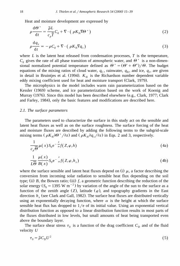
Ž . Ž . Ž .Fig. 1. yz-cross-sections of the surface m a , B b and z c are shown by the shaded area. The topography0

is outlined by the solid line. The length of the domain in indicated in km on the x-axis, the y-axis on theleft-hand side gives the scale for the conversion rate, the Bowen ratio, and the roughness lengths z in m. The0

y-axis on the right-hand side gives the scale for the topography in m.

. Ž .increased likelihood of thunderstorms is 27 , and the Boyden 1963 index is 96Ž .threshold 94 . The profile is moist up to a height of about 5 km, then topped by acomparatively drier layer. The total precipitable water in the air column from cloud baseto cloud top is 40.7 mm.

The winds on June 27, 1990 were southwesterly in the lower troposphere, andwesterly throughout the rest of the atmosphere, showing steadily increasing wind speedsfrom 1.5 mrs at the surface to 25 mrs at 9 km. For the 2D study, the observed windprofile has been modified to account for the restricted westerly flow. The wind speedshave been slightly reduced, and increase steadily from 0.5 mrs at the surface to amaximum of 22 mrs at 9 km.

The model simulations are started 2 h prior to the sounding, and therefore, thetemperature and dew point values of the midday profile have been slightly cooled in theboundary layer to account for the earlier simulation time.


Fig. 2. Skew-T diagram of the temperature, dew point and wind profile used to initialize the meteorologicalmodel. Height in km and pressure levels in hPa are indicated on the left-hand side of the diagram, dry bulbtemperature is indicated at the right-hand side.

3.3. Initialization of soil parameters and the surface

A high resolution land-use data set was provided by the Institut Geographique´National de France for the area of Ile de France, a region of approximately 130 km2 innorthern France. From this data set, 10 different soil classes are constructed, and each is

Ž .then assigned typical values for m, B, and z . In the case of the Bowen ratio B and0Ž .the roughness length z , these are extracted from standard references such as Oke0

Ž . Ž .1987 or Stull 1988 . The estimation of the conversion factor from incoming solarŽ .radiation to sensible heat flux, m, is based on results of Clark and Gall 1982 and

Ž .Thielen and Gadian 1996 .For the 2D studies, non-averaged west–east cross-sections intersecting the city centre

of Paris have been extracted from the complete data set. Fig. 1 shows the cross-sectionsof the three surface parameters across the whole model domain. The urban area issituated roughly between 50 and 90 km, and is surrounded by less urbanized or ruralareas. Fig. 1a and b illustrate that for this cross-section, up to 37% of the incoming solarradiation is converted to sensible heat flux over the urban area, while over rural areas


Ž .this conversion can be up to 20% lower. The height a Eqs. 4a and 4b , at which thesurface sensible fluxes have decreased to 1re of their initial values is set to 500 m. Thevalue of the surface roughness length, shown in Fig. 1c, increases from 20 cm in therural areas to maximum values of nearly 2 m in the city centre. On the outflowboundary, no detailed surface data are available from 120 km onwards, and therefore aconstant, representative of the rural environment, is applied.

The ranges of m, B, and z for the different surfaces are shown in Table 1.0

For the following model studies, we assume that each surface parameter can have twodifferent configurations.

Ž .a The surface parameter is constant throughout the length of the domain. This isdenoted with a C. The constant values have been chosen more or less arbitrarily, but aretargeted to represent the threshold value between rural and urban conditions. Valuesused are ms0.28, Bs0.8, and z s0.2 m.0

Ž .b The surface parameter varies spatially as illustrated in Fig. 1a–c by the shadedcurve. It describes a rural environment including an extended urban area of about 40 kmin diameter. This is the so-called ‘urban’ set-up and is denoted with a U.

3.4. Boundary conditions and filters

The model is set up with open lateral boundary conditions, and free-slip upperboundary conditions, using an 8-km deep Rayleigh friction absorber layer to dampenreflection of waves at the artificial upper boundary. The surface is treated as a no-slipboundary. A Robert–Asselin time filter is applied to prevent the development ofnumerical instabilities due to the time-centred differencing schemes.

3.5. Presentation of the different simulations

The notation for the different runs is a composite of the two letters C or U. The firstletter stands for the sensible heat flux parameter m, the second for the Bowen ratio B,and the third for the roughness length z . For example, CCC denotes the control run0

where all parameters are kept constant, UCC denotes the simulation where only thesensible heat flux parameter varies while all the other parameters are kept constant. Inorder to exclude superposition of soil forcing with topography-related effects such asdifferential slope heating, varying terrain is only considered in a few explicit runs. In

Ž .these cases, the same configuration as for the control run CCC and the urban run

Table 1Ž .Values used for the calculation of the conversion rate of incoming solar radiation to sensible heat flux m , the

Ž . Ž .Bowen ratio B , and the roughness length z0

Ž .Type of surface m B z m0

City centre, tall buildings 0.30–0.40 1.5–3.0 1.0–2.0Urbanized areas, villages 0.25–0.30 0.8–1.5 0.5–1.0Forest, open grassland 0.20–0.30 0.2–0.8 0.2–0.5Lakes, rivers 0.10–0.20 0.1–0.2 0.001–0.2


Table 2Description of the different simulations for the three parts including the name of the simulations, the minimumand maximum values for the surface parameters m, B, and z as used in the simulations0

Ž .Simulation m B z m0

Part ICCC 0.28 0.8 0.2UUU 0.10–0.40 0.2–2.0 0.2–2.0

Part IIUCC 0.10–0.40 0.8 0.2CUC 0.28 0.2–2.0 0.2CCU 0.28 0.8 0.2–2.0

Part IIITOPC like CCC but with topographyTOPU like UUU but with topography

Ž .UUU are used combined with topography. They are denoted as TOPC and TOPU,respectively. The different simulations are listed in Table 2.

The presentation of results is divided into three parts. The first part describes acomparison between the control run CCC and the most realistic run UUU, where allsurface parameters vary spatially. In Part II, the relative importance of the individualparameters for the atmospheric processes is discussed for the sensible heat flux

Ž . Ž . Ž .parameter UCC , the Bowen ratio CUC , and the roughness length CCU . The thirdpart addresses the additional influence of topography by comparing results betweenTOPC and CCC, and between TOPU and UUU.

4. Results

The spin-up time varies for the different simulations and is the shortest for the‘‘urban’’ run at 80 min, and the longest for the control run at 95 min. The analysis istherefore focused on integration times of longer than 100 min.

Rainfall data have been calculated at the surface. All other data presented in thefollowing analyses, such as fluxes and vertical velocity, are a mean of data at the surfaceand the next grid point at 40 m.

4.1. Part Ia: comparison between the control run CCC and the urban run UUU

Fig. 3a shows the accumulated rainfall over the last 3 h of simulation CCC. Themaximum amounts to 12.7 mm, with an average rainfall total of 2.3 mm, and a standarddeviation of 3.1. The curve shows that there are two local maxima located at around 35and 165 km, which are of comparable strength, and which vary between 10 and 12 mm.In the centre of the domain rainfall totals are low.

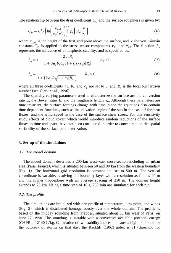
The temporal development of the surface rainfall for CCC is summarized in Fig. 4.The spatial co-ordinate, showing the horizontal length of the domain, is presented on the


Ž . Ž .Fig. 3. Rainfall totals for CCC a and UUU b , accumulated from 100 to 250 min of simulation and averagedover 10 grid points. The rainfall total is given in mm, the x-axis gives the distance from the western boundary

Ž .in km. The location of the urban surface is indicated by two dashed lines in b .

x-axis, and the time is shown on the y-axis. Rain cells progressing from west to east arethus illustrated by diagonally orientated patches, where the horizontal width of the patchgives the spatial extent of the rainwater content field, and the vertical length the durationof these cells. The rainfall intensity is given by the grey-scale next to the diagram.

Ž .As could be expected from earlier studies e.g., Hill, 1974 , the homogeneous heatingat the ground produces a superadiabatic lapse rate which destabilizes the air above theground. Subsequently, first a sub-cloud circulation with regularly spaced up and

Ž .downdraught regions is initiated prior to the development of clouds not shown . Withinthe stronger updraughts of this circulation, small convective clouds with an averagewidth of 2–3 km develop about 100 min throughout the length of the domain. Althoughmost of them contain rainwater, they are small, with an average width of 2–3 km.

Ž .Except for the rainfall cell at 30 km east see Fig. 4A , most other cells only produceŽ .traces of rainfall -0.3 mmrh and last for less than 10 min.

Small and short-lasting cells are formed continuously after 100 min throughout thesimulation. But the airflow is increasingly dominated by the cloud convection anddowndraughts caused by the precipitation, which results in convective cells, which areorganized on larger space and time scales than during the first 100 min of simulation.

Ž . Ž . Ž .Larger cells occur at 100 min a , 170 min b , and 210 min c , at an average spacing of


Fig. 4. Distance and time-plot of the rainfall intensity for the control simulation CCC. The distance is shownon the x-axis in km, and the simulation time on the y-axis in min. The rainfall intensity is given in mmrh. Alower cut-off level of 1 mmrh is chosen allowing a better presentation of the isolated precipitation cells. Thecontour lines are drawn in 1, 5, 10, 20, 30 and G50 grkg. The grey shades are defined by the grey scale nextto the diagram.

60–80 km. The larger rainfall fields average 15–20 km in width, and last between 30and 60 min. At some locations, repeated formation of rainfall is observed, e.g., around

Ž . Ž .30 km A and 160 km C . To some extent, re-occurring rainfalls are also simulated atŽ . Ž110 km B , but those cells are weak and do not result in increased rainfall totals Fig.

.3a .The total accumulated rainfall for simulation UUU is shown in Fig. 3b. Obviously,

the rainfall patterns are strongly influenced by the variable surface parameterizationscheme, and switching on of all surface parameters results in rainfall enhancement andre-organization of the rainfall fields. As compared to CCC, the rainfall is focused overthe urban surface and at a distance of 60–80 km downwind of it. Unlike in CCC, hardlyany rainfall is simulated west of the ‘‘urban’’ area. The maximum rainfall, located overthe eastern part of the ‘‘urban’’ area, is 13 mm greater than in the control run, andamounts to 26 mm. The average rainfall is with 6.3 mm more than twice as high as inCCC, and also the standard deviation is significantly higher with 7.6.

Ž .Fig. 5 shows the surface sensible heat fluxes solid and the surface latent heat fluxesŽ . Ždotted at noon, spatially averaged over 5 km for simulation UUU and also UCC for

.the sensible heat fluxes and CUC for the latent heat fluxes . Since no topography isconsidered, they are obviously closely related to the input parameters given in Fig. 1.


Ž . Ž .Fig. 5. Surface sensible solid line and surface latent heat fluxes dashed line at noon for simulation UUU.The distance from the western boundary is given on the x-axis in kilometers, the strength of the heat fluxes inW my2 . The data is averaged over 10 grid points.

The surface latent heat fluxes show the largest variability, and range from 100 W my2

over the urban area to 575 W my2 over rural parts. In comparison, the surface sensibleheat fluxes range only between 200 and 350 W my2 . Towards the outflow boundary ofthe domain, where the surface parameters do not vary spatially, the fluxes remain at aconstant value of 330 W my2 for the latent heat fluxes and 275 W my2 for the sensibleheat fluxes. These are the same values for simulation CCC across the whole domain.The urban area is clearly characterized by an increase in surface sensible heat flux of100 W my2 and a reduction in surface latent heat flux of an average of 200 W my2 .The average value of the surface sensible heat fluxes amounts to 270 W my2 over therural areas and to 324 W my2 over the urban area. In contrast, the average surface latentheat fluxes amount to 350 W my2 over the rural areas and to 170 W my2 over theurban area. The overall average of the surface latent heat fluxes is 35 W my2 higherthan that of the surface sensible heat fluxes. Comparing with data from the literatureŽ .e.g., Stull, 1988 , it appears that the variation and magnitude of the surface sensibleheat fluxes agree well with mid-June conditions, while the surface latent heat fluxes maybe slightly overestimated over some rural areas.

The increased surface sensible heat flux over the urban area produces increasinglyhigh-reaching convection, resulting in the development of rainwater within 80 min atthis location. This is illustrated in Fig. 6, which shows the temporal development of the


Fig. 6. Distance and time-plot of the rainfall intensity for the simulation UUU. The two dashed lines indicatethe approximate limits of the urban surface to the West and the East. Axes and grey scale same as Fig. 3.

rainfall fields. Compared to the control run CCC, the development of rainwater occursabout 30 min earlier. The cells are generally 30–50% larger and longer-lasting than withconstant surface parameters, and the number of small and short-lasting cells is alsoconsiderably reduced.

The precipitation becomes spatially focused at two locations, and re-occurringŽ .rainfalls appear over the urban surface forcing area A , indicated roughly by the two

Ž .dashed lines in Fig. 6, and about 60 km downwind of it B . Repeated formation of raincells occurs particularly at the eastern and leeward part over the urban area, for instanceat 90, 120, 150, and 180 min, resulting in higher accumulated rainfall over this regionŽ . Ž . Ž .26 mm than elsewhere in the domain Fig. 3 . Over the western windward parts, therainfall is comparatively low. At 70 km downwind of the urban area, a long-lasting cellŽ .)100 min with several regions of increased convective rainfall is formed at 80 min.

Ž .Towards later stages of the simulation around 200 min , another smaller and shorter-lasting cell is triggered at the same location.

Fig. 7 shows the vertical wind averaged over the last 3 h of the simulation, from 100Ž . Ž .to 240 min, for simulation CCC a and UUU b . Spatially, the data have been averaged

over 4-km strips. Descending winds have a negative sign. The location of the urban areaŽ .is marked by the two dashed lines in b .


Ž .Fig. 7. Vertical wind speed averaged over a time period from 100 to 250 min for simulation CCC a and UUUŽ .b . Spatially, the data have been averaged over 10 grid points. Descending winds have a negative sign. The

Ž .location of the urban area is marked by the two dashed lines in b .

In CCC the average vertical winds fluctuate around zero across the domain, showingonly a light periodicity in magnitude at a distance of 40 to 50 km. The three localmaxima coincide approximately with the location of the three regions of repeated

Ž .rainfall Fig. 4 .Unlike in the control run, in simulation UUU the average winds are mostly ascending

and less fluctuating. Two particular regions can be distinguished.Ž .a Over the urban region, the airflow is ascending west, windward of the urban area,

and descending in the east, on the leeward side. This airflow pattern is mostly aconsequence of the urban heat island. The buoyant air rises over the heated surface,causing convergent winds in the lower boundary layer. The inflowing air becomes thentransported upwards to cloud base. Depending on the strength of the updraughts and thelocal cloud environment, conversion from cloud water to rain and ice is initiated, whicheventually falls out in the compensating downdraught region over the leeward parts of

Ž .the urban area Fig. 6 .Ž .b The second region corresponds to the area of increased convective activity

downwind of the city centre, and is characterized by large variations of w. The urbanarea represents an obstacle to the air flow because it initiates the rising of buoyant airand it enhances the turbulence of the flow due to increased surface roughness. The largevariations of w are at least partly induced by the wake structure of the air flow


downwind of the obstacle. It is likely that within a 3D framework, these waves would beless apparent.

4.2. Part Ib: comparison between the control run UUU and obserÕational data

The initialization profile was taken on June 27, 1990, a day of important convectiveactivity in the Paris region. During the afternoon of June 26, 298C was measured in thecity centre, while the temperatures in the rural surroundings were about 38C cooler.During the night, moist air from the southwest was advected into the area, andthunderstorms developed and caused heavy rainfall over Paris.

Ž .Fig. 8 shows the isohyets of the rainfall totals for the night of 26r27 June a and forŽ .the afternoon of June 27 b as deduced from gauge data. The dots show the positions of

the rain gauges, and the dashed lines indicate the boundaries of Paris, the dense urbanarea typical of large city centres, and of Seine-Saint-Denis a less urbanized countyNortheast of Paris.

Fig. 8a shows two areas of high rainfall totals of 30 mm, one centred over Paris, andone about 25 km downwind of it, affecting the western parts of Seine-Saint-Denis.During the afternoon of June 27, another storm approached the area, again from thesouthwest. The rainfall was higher than in the previous storm and produced totals of 50

Ž .mm Fig. 8b . Again, two regions of equally intense rainfalls were observed, one overŽ .the northeastern leeward side of the city centre, and the second one about 20 km

Ždownwind of it, causing serious flooding in the area of Seine-Saint-Denis Thielen and.Creutin, 1997 . Over the southwestern and windward side of the city centre of Paris, a

rainfall of lower than 20 mm was observed.Ž .Qualitatively, the analysis of the two storms agrees with simulation UUU on a theŽ .tendency of low rainfalls over the windward part of the city centre, and b the

occurrence of two equally strong local rainfalls, one located over the leeward side of thecity, and one at a considerable distance downwind of it.

Quantitatively, the magnitude of the simulated rainfall totals of 26 mm in UUU arelower than the observed ones, in the case of the last storm, by a factor 2. Although at afew occasions the simulated maximum rainfall intensities in UUU exceed 100 mmrh,the rainfall totals remain low because of the short duration of the cells. There are severalfactors which could cause the underestimation of the rainfall, e.g., the parameterizationof the microphysics, in particular of the ice phase, which plays an important role inhigh-reaching convective storms in our latitudes, or the lack of directional wind shear

Ž .which is an important feature of convective storms Browning and Ludlam 1962 , toname a few.

Larger discrepancies become apparent when comparing the distances between theurban area and the increased rainfall downwind of it. In both storms, the observeddistance on June 27 is only half the distance simulated. The observations on June 27 are

Ž .supported by Escourrou 1991 , who also found for Paris a typical distance between twoareas of increased rainfall of 20–30 km. It is likely that the overestimation of thisdistance is also an effect of the 2D simulations, since the air flow is not able to goaround obstacles as would be possible in a 3D framework, having consequences on thewake structure downwind of the perturbation.


Compared to the observations from METROMEX, the results for UUU are also inqualitative agreement. It was concluded that large urban areas have impact on the

Ž .frequency of convective storms Huff and Vogel, 1973; Chagnon, 1978 . Storms tendedto occur twice as often over urban agglomerations relative to comparable rural areas.Heavy rain bearing cells exposed to the urban environment yielded 70% more precip-

Ž .itable water than comparable cells in rural regions Huff, 1977 . Rainfall enhancementwas observed at an average distance of 40 km downwind of the city centre, a largerdistance than observed for the Paris region. It is likely that this is due to the largerextension of urbanized areas in the US relative to Europe, and Paris in particular.

The relative importance of the individual parameters is now studied by switching ononly one parameter at the time.

4.3. Part II: relatiÕe importance of the three indiÕidual surface parameters

( )4.3.1. Influence of the conÕersion rate m UCCŽ .Fig. 9a shows the rainfall totals for simulation UCC solid line . For comparison, the

Ž .data for UUU are also plotted dotted line .Variation of only the conversion rate m results in similar precipitation patterns as in

UUU where all the three parameters vary spatially. As compared to UUU, the maximumŽ .rainfall over the urban area 20.6 mm is shifted slightly to the west, and rainfall east of

the urban surface is higher. For example, at 125 km, no rainfall is simulated for UUU,while an average of 10 mm is simulated for UCC. Particularly towards later stages of thesimulation, after 200 min, the rainfall fields become slightly larger and with moreindividual convective cells embedded than in UUU, and overall, a higher number ofsmall and short-lasting rain cells are simulated.

The few differences between the runs UCC and UUU seem to indicate that with thepresent set-up the surface sensible heat flux is the dominant forcing of the rainwaterdevelopment. This is not surprising because the underlying configuration is based on anunstable environment, weak winds and wind shears, and no topography, leaving positivebuoyancy as the dominant forcing to trigger convection.

These results support the observations that urban heat islands can influence convec-tive rainfall development. Additional simulations that are not presented in this paperindicate that the stronger the heat island intensity, the more pronounced the effects are inthe vicinity of the forcing area, while weak heat islands mostly favour increased rainfallsat some distance downwind of the heated surface.

( )4.3.2. Influence of the Bowen ratio CUCVariation of the Bowen ratio produces similar rainfall patterns as control run CCC.

Ž .This is illustrated in Fig. 9b, which shows the total rainfall for CUC solid black line

Ž .Fig. 8. Isohyets of rainfall totals as interpolated by gauge data for a the storm during the night from June 26Ž .to 27, and b for the storm during the afternoon on June 27. The dots indicate the location of the gauges

Ž .climatological network of Meteo-France , the dashed lines show the boundaries of the county of Paris and the´ ´county of Seine-Saint-Denis.


Ž . Ž . Ž .Fig. 9. Rainfall totals accumulated from 60 to 250 min of simulation for UCC a , CUC b , and CCU cŽ .drawn in solid lines. For comparison, the rainfall totals of UUU are drawn as a dotted line in a , and of CCC

Ž . Ž .in b and c , respectively. The rainfall totals are given in mm, the x-axis gives the distance from the westernboundary in km. Data are averaged over 10 grid points.

Ž .and CCC dotted grey line . As compared to CCC, the variable Bowen ratio results in aŽ .slight decrease of rainfall over and downwind of the urban surface 95–115 km , and a

small increase of water content towards the end of the simulations.Since the only difference between the two runs consists in the variation of the Bowen

ratio, the differences in latent heat fluxes between CCC and CUC are examined next.Fig. 10 shows the spatial distribution of the latent heat flux 10 m above the surface,

Žaveraged from 150 to 180 min at a sampling frequency 10 s, for simulation CCC dotted. Ž .line and simulation CUC solid line . During this time interval, light convection is

Ž .present across the domain Fig. 4 . The data are spatially averaged over 10 grid points.As could perhaps be expected, there are no striking differences between the two cases.In CCC, the latent heat flux appears to fluctuate randomly between "200 W my2

across the domain and no particular region of high or low activity can be distinguished.In CUC, the fluctuations are of the same magnitude as in CCC.

ŽIt appears that sharp changes in latent heat fluxes as indicated in Fig. 5 e.g., at 20, 40.or 90 km , induce locally a slightly higher variability in the data. The biggest difference


Fig. 10. Spatial distribution of the time-averaged subgrid-scale latent heat flux at 10 m above the surface forŽ . Ž .simulation CCC top and simulation CUC bottom . The distance from the western boundary is given on the

x-axis in km, the strength of the heat fluxes in W my2 . The data are averaged over 10 grid points.

between the two curves can be observed over the urban area and towards the outflowboundary where the time averaged fluxes are lower and less variable than in the controlrun CCC. These differences in latent heat fluxes, however, are not reflected in the

Ž .rainfall development within the same time interval not shown . The reduction of rainfalldownwind of the urban area as shown in Fig. 9b, is produced from 200 min onwardsonly. The rainfall cell developing at 215 min located at 85 km from the inflow boundary

Ž .in CCC Fig. 4 is absent in CUC, and the cell at 235 min located at 105 km is muchweaker in CUC than in CCC, producing the lower rainfall totals in that area. The slightincrease of rainfall towards the outflow boundary in CUC is due to slight differences inrainfall from 170 min onwards, showing a small tendency of higher rainfalls in CUCthan in CCC.

Therefore, it seems that sudden changes of the Bowen ratio at the surface mayproduce local changes in latent heat fluxes. Reduction of surface latent fluxes of 200 Wmy2 from rural to urban areas results in lower average latent heat fluxes in the lowerboundary layer. The reduction of average latent heat fluxes, however, does not seem tobe coupled to an instantaneous reduction in rainfall. Significant rainfall differences occuronly towards the end of the simulations. It therefore seems that under convectiveconditions, local variations of the surface latent heat flux need more than 3 h to become


effective, and thus, have little effect on rainfall processes within the considered time andlength scales.

One should note that the Bowen ratio has been kept constant in time throughout thesimulations, which does not take into account the evaporation of rainwater accumulatedover impermeable surfaces. In urban boundary layer studies, the latent heat flux is,therefore, an important variable for the urban climate. However, the reaction ofconvective rainfall processes to spatial variations in the latent heat fluxes seems slow,and in these relatively short simulations, it can be assumed that even a time-dependentBowen ratio would not significantly modify the results.

( )4.3.3. Influence of the roughness length CCUIn this section, the effects of surface roughness changes on rainfall is assessed.

Differences in total rainfall upwind of the urban surface between CCU and CCC areŽ .small Fig. 9c , and only a light increase of rainfall of about 8–10 mm directly over the

urban surface is simulated. In CCU, the highest rainfall totals are located between 130and 150 km, 50–70 km downwind of the urban surface. In fact, with a maximum of 28.8mm, this represents the highest rainfall total of all simulations. This suggests that aperturbation of the atmospheric flow through increased surface roughness may lead toenhanced rainfall at some distance downwind of the perturbation zone.

Ž .Analyses of the temporal development of the rainfalls not shown show that theinfluence of the increased turbulence over the urban surface becomes most effectiveafter 3 h, and downwind of the increased surface roughness. The increased drag over theurban surface results in a slowing down of the air flow, which produces a localconvergent wind field. The inflowing air is forced to rise, not as energetically as buoyantair, and after some time reaches the cumulus convection level at some distance

Ždownwind of the perturbation. Additional studies with different cut-off levels for z not0.shown suggest that there is a relationship between roughness height and rainfall

intensities. The higher the roughness height, the higher the rainfall downwind of theperturbation.

The main forcing on convective processes in this case is the increase of subgrid-scaleX Xturbulence in the lower levels. Fig. 11 illustrates the differences in Reynolds stress ru w

Ž .average between surface and the first grid point above for the two simulations CCCŽ . Ž .dotted line and CCU solid line . The Reynold stress is averaged over the last 150 minof simulation and spatially averaged over 10 grid points.

In both cases, the Reynold stress fluctuates around zero across the domain, withlarger variations toward the western boundary, which is probably an effect of theinflowing air. The most significant difference between the two curves is the much largervariation of the Reynold stress towards the outflow boundary in CCU, where maximum

2 Ž .variations of "0.8 Nrm from 175 km onwards are simulated, as opposed to "0.3Nrm2 in CCC. This region of large variability coincides with the region of increasedconvective rainfall, as illustrated in Fig. 9c.

These results suggest that in 2D the precipitation enhancement can also be a functionof the differences of the roughness height. In 3D simulations, however, where the airflow has the possibility to go around an obstacle, the effect of roughness changes on theprecipitation intensity might be considerably reduced. Based on observational data,


X X Ž . ŽFig. 11. Reynolds stress ru w close to the surface for the two simulations CCC dotted line and CCU solid. 2 Ž .line . The Reynold stress, given in Nrm , is averaged over the last 150 min of simulation 100 to 250 min

and spatially averaged over 10 grid points. The distance from the western boundary is given in km.

Ž .Escourrou 1991 estimated the influence of roughness on the development of precipita-tion in the region of Paris, and her results qualitatively confirm the simulations. Forsouthwesterly winds, she observed an increase of precipitation from the outskirts ofParis onward, and particularly an increase in the northern parts of the city, downwind ofthe downtown area. A precipitation enhancement due to roughness of 10% is quoted, butit is not clear if this is a general value or if it refers explicitly to the Paris region.

( )4.4. Part III: influence of topography TOPC, TOPU

Ž .Irregular terrain has been added to the simulation set-ups of CCC denoted as TOPCŽ .and UUU denoted as TOPU . The rainfall totals for both simulations are shown in Fig.

12 and compared against CCC and UUU, respectively.In simulation CCC the topography is absent, and the surface forcings are constant

across the domain. Therefore, first computational instabilities due to round-off errorsneed to develop and amplify before the perturbations are important enough to establishconvective circulation patterns. Inclusion of topography produces from the very begin-ning local variations in the pressure, wind and temperature fields through upslope liftingand increased drag. Owing to the generally flat topography, no important temperaturedifferences between sun facing and shadowed slopes can develop on the given timescale.


Ž . Ž .Fig. 12. Rainfall totals accumulated from 100 to 250 min of simulation for TOPC a , and TOPU b drawn inŽ .black solid lines. For comparison, the rainfall totals of CCC are drawn as a grey dotted line in a , and of UUU

Ž .in b . The rainfall totals are given in millimeters, the x-axis gives the distance from the western boundary inkm. The data are averaged over 10 grid points.

Consideration of topography results in earlier onset of rainfall development, reductionof small and short-lasting cells, and enhanced rainfall intensities towards the outflow

Ž . Ž .boundary not shown . Although the topography gradients are weak 1r300 m , it seemsthat in TOPC enhanced rainfall is simulated just upwind of the slightly elevated terrain

Ž .80 km east of Paris compare Fig. 1 and Fig. 12a .It is possible that, again, the influence of the surface drag on the atmospheric

processes has been overestimated in the 2D framework, contributing to the increasedrainfalls downwind of the urban surface, similar to simulation CCU. A comparison studyin 3D is envisaged as possible future work to clarify this point.

As compared to UUU, in TOPU cells are slightly smaller and shorter-lasting. Therainwater is again focused over the urban area owing to re-occurring rainfalls. Thebiggest difference is that the enhanced rainfall downwind of the urban heat island is

Ž .considerably weaker than in UUU Fig. 12 . This is somewhat contradictory to thefindings for TOPC, where the effects of topography resulted in increased rainfall atsome distance downwind of the urban surface. Thus, it seems that the modification ofthe atmospheric processes due to the surface are complex and manifold, and interactionsof the different influences make their global effects very difficult to predict. Forsimulations aimed at reproducing particular case studies, the representation of the


surface can play an important role both for quantity as well as the spatial distribution ofthe rainfall.

5. Conclusions

In the present study, a spatially variable parameterization scheme for the surfacesensible heat flux, the surface latent heat flux, and the roughness is introduced into ameso-scale numerical model. The results indicate that the surface conditions should notbe neglected and can have considerable influence on meso-scale processes such asconvective rainfall.

On a relatively short time scale of less than 4 h, it is mainly the surface sensible heatfluxes and subsequent buoyancy variations that influence the rainfall development.Inclusion of heat islands result in increased rainfall over and at a certain distancedownwind of the heat island. The stronger the heat island intensity, the more pro-nounced the effects are in the vicinity of the forcing area, while weak heat islands favourincreased rainfalls only at some distance downwind of the heated surface. Therefore, inorder to produce realistic simulations, a correct initialization of the surface temperatureand the surface sensible heat fluxes is most important.

The influences of local changes in the surface latent heat fluxes are comparativelyslow acting and do not show significant effects within the 4 h of simulation. This is notsurprising in this case, because the basic state of the atmosphere is chosen to be unstableand moist in the lower levels. It also seems that the parameterization of the Bowen ratioshould be recalibrated since average values of latent heat fluxes appear low relative tothe sensible heat flux in the given rural conditions.

Changes in the roughness length modify the precipitation patterns significantlydownwind of the urban surface in these 2D simulations. The effects develop only after2–3 h of simulation, and seem to be a function of the height of the roughness lengths,although this may well not apply for 3D simulations. However, in combination with avariable sensible heat flux, the buoyancy forces dominate the precipitation development.Similar conclusions could be drawn for those simulations that include topography.Because the topographical gradients are small, the artificially induced heat islandsthrough urbanization remain the dominant surface forcing.

Overall, the results seem to confirm observations, such as those from theMETROMEX experiment, that the frequency distribution of rain-bearing cells is en-hanced over urban areas, and that precipitation can be enhanced by the presence ofurban agglomerations.

For a more realistic assessment of the effect of these parameters on rainfalldevelopment, and for a quantitative comparison with observations, the simulationsshould be performed in three dimensions. 2D simulations represent a limitation for therepresentation of the dynamical response of the atmosphere to turbulent processesrelated to cloud formation and precipitation, which are essentially 3D. Further, the timedependency of the soil conditions should not be neglected. A next step will thereforeinclude a soil model to calculate the surface temperatures and moisture contents at eachtime step dependent on soil conditions.


Acknowledgements

The authors would like to thank T.L. Clark and W.D. Hall for the permission to useŽ .their code. One of the authors J.T. acknowledges the financial support given by the

Conseil Regional des Pays de la Loire and the Programme de Recherche en Hydrologie´Ž .No. Contract INSU_CNRS 94PRH19 . We thank the Institut Geographique National´for providing the topography land-use data, and the Departement de l’Eau et de´l’Assainissement de la Seine-Saint-Denis for the rainfall data.

References

Bornstein, R.D., 1986. Urban climate models; nature, limitations and applications. In: Urban Climatology andits Applications with Special Regard to Tropical Areas. pp. 237–276, WMO-No.652, Geneva.

Boyden, C.D., 1963. A simple instability index for use as a synoptic parameter. Meteorol. Mag. 92, 198–210.Braud, I., Dantas-Antonino, A.C., Vauclin, M., Thony, J.L., Ruelle, P., 1995. A simple soil-plant-atmosphere

Ž .transfer model SiSPAT : development and field verification. J. Hydrol. 166, 213–250.Browning, K.A., Ludlam, F.H., 1962. Airflow in convective storms. Q. J. R. Meteorol. Soc. 88, 117–135.Bruintjes, R.T., Clark, T.L., Hall, W.D., 1994. Interactions between topographic airflow and cloudrprecipita-

tion development during the passage of a winter storm in Arizona. J. Atmos. Sci. 51, 48–67.Chagnon, S.A., 1978. Urban effects on severe local storms at St. Louis. J. Appl. Meteorol. 17, 578–586.Changnon, S.A., Huff, F.A., Schickedanz, P.T., Vogel, J.L., 1977. Weather anomalies and impacts. In:

Summary of METROMEX Vol. I Ill. State Water Survey, Bull. 62, Champaign, 260 pp.Clark, T.L., 1977. A small-scale dynamic model using a terrain following coordinate transformation. J.

Comput. Phys. 24, 186–215.Clark, T.L., 1979. Numerical simulations with a three-dimensional cloud model: lateral boundary condition

experiments and multi-cellular severe storm calculations. J. Atmos. Sci. 34, 2191–2215.Clark, T.L., Farley, D., 1984. Severe downslope windstorm calculations in two and three spatial dimensions

using anelastic interactive grid nesting: a possible mechanism for gustiness. J. Atmos. Sci. 41, 329–350.Clark, T.L., Gall, R., 1982. Three-dimensional numerical simulations of airflow over mountainous terrain: a

comparison with observations. Mon. Weather Rev. 110, 766–791.Clark, T.L., Grabowski, W.W., 1991. Cloud-environment interface instability, rising thermal calculations in

two spatial dimensions. J. Atmos. Sci. 48, 527–546.Clark, T.L., Hall, W.D., Coen, J., 1996. Source code documentation for the Clark-Hall cloud-scale model,

code version G3CH01; NCARrTN-426qSTRNCAR Technical Note, May 1996, NCAR, Boulder, CO,USA

Draxler, R.R., 1986. Simulated and observed influence of the nocturnal urban heat island on the local windfield. J. Clim. Appl. Meteorol. 24, 1125–1133.

Escourrou, G., 1991. Le climat de la ville, Nathan, Paris. 187 pp.Goldreich, Y., 1995. Urban climate studies in Israel, a review. Atmos. Environ. 29, 467–478.Hill, G.E., 1974. Factors controlling the size and spacing of cumulus clouds as revealed by numerical

experiments. J. Atmos. Sci. 31, 636–673.Huff, F.A., 1977. Urban effects on storm rainfall in midwestern United States. In: Proc. Amsterdam

Symposium, Oct. 1977 Vol. 123 IAHS-AISH, pp. 12–19.Huff, F.A., 1986. Urban hydrological review. Bull. Am. Meteorol. Soc. 67, 703–712.Huff, F.A., Vogel, 1973. Precipitation modification by major urban areas. Bull. Am. Meteorol. Soc. 54,

1220–1232.Kessler, E., 1969. On the distribution and continuity of water substance in atmospheric circulations. Meteorol.

Monogr. 32, 84.Koenig, L.R., Murray, F.W., 1976. Ice-bearing cumulus cloud evolution, numerical simulation and general

comparison against observation. J. Appl. Meteorol. 15, 747–762.


Lee, T.J., Pielke, R.A., Kittel, T.G.F., Weaver, J.F, 1993. Atmospheric modelling and its spatial representationŽ .of land surface characteristics. In: Goodchild, M.F., Parks, B., Steyaert, L.T. Eds. , Integrating Geo-

graphic Information Systems and Environmental Modelling. Oxford Univ. Press, pp. 108–122.Loose, T., Bornstein, R.D., 1977. Observations of mesoscale effects on frontal movements through an urban

area. Mon. Weather Rev. 105, 563–571.Moussiopoulos, N., 1994. In: The EUMAC Zooming Model, Model Structure and Applications. EUROTRAC

International Scientific Secretariat, Garmisch-Partenkirchen, March.Noilhan, J., Planton, S., 1989. A simple parameterization of land surface processes for meteorological models.

Mon. Weather Rev. 117, 536–549.Oke, T.R., 1987. Boundary Layer Climates. Chapman & Hall, Routledge, London, 435 pp.Pielke, R.A., 1984. Mesoscale Meteorological Modelling. Orlando Press, 612 pp.Pielke, R.A., Dalu, G., Snook, J.S., Lee, T.J., Kittel, T.G.F., 1991. Nonlinear influence of mesoscale landuse

on weather and climate. J. Clim. 4, 1053–1069.Rackliff, P.G., 1962. Application of an instability index to regional forecasting. Meteorol. Mag. 91, 113–120.Rotach, M.W., 1993a. Turbulence close to a rough urban surface: Part I. Reynolds stress. Boundary Layer

Meteorology 65, 1–28.Rotach, M.W., 1993b. Turbulence close to a rough urban surface: Part II. Variances and gradients. Boundary

Layer Meteorology 66, 75–92.Sievers, U., Forkel, R., Zdunkowski, W., 1983. Transport equations for heat and moisture in the soil and their

application to boundary layer problems 1983. Beitr. Phys. Atmos. 56, 53–83.Stull, R.B., 1988. An Introduction to Boundary Layer Meteorology. Kluwer Academic Publishing, Nether-

lands, 666 pp.Theurer, W., Baechlin, W., Plate, E.J., 1992. Model study of the development of boundary layers above urban

areas. J. Wind Eng. Ind. Aerodyn. 41–44, 437–448.Thielen, J., Creutin, J.-D., 1997. An urban hydrological model with high spatial resolution rainfall from a

meteorological model. J. Hydrol. 200, 58–83.Thielen, J., Gadian, A., 1996. Influence of different wind directions in relation to topography on the outbreak

of convection in Northern England. Ann. Geophys. 14, 1078–1087.Vukovich, F.M., Dunn, J.W., 1978. A theoretical study of the St. Louis Heat Island: some parameter

variations. J. Appl. Meteorol. 17, 1585–1595.

the possible influence of urban surfaces on rainfall ...directory.umm.ac.id/data...

Documents