the polynomial method strikes back: tight quantum … polynomial method strikes back: tight quantum...
TRANSCRIPT

The Polynomial Method Strikes Back:
Tight Quantum Query Bounds via Dual Polynomials
Mark BunPrinceton [email protected]
Robin KothariMicrosoft Research
Justin ThalerGeorgetown University
Abstract
The approximate degree of a Boolean function f is the least degree of a real polynomial thatapproximates f pointwise to error at most 1/3. The approximate degree of f is known to be alower bound on the quantum query complexity of f (Beals et al., FOCS 1998 and J. ACM 2001).
We resolve or nearly resolve the approximate degree and quantum query complexities ofseveral basic functions. Specifically, we show the following:
• k-distinctness: For any constant k, the approximate degree and quantum query complexityof the k-distinctness function is Ω(n3/4−1/(2k)). This is nearly tight for large k, as Belovs(FOCS 2012) has shown that for any constant k, the approximate degree and quantum
query complexity of k-distinctness is O(n3/4−1/(2k+2−4)).
• Image Size Testing: The approximate degree and quantum query complexity of testing thesize of the image of a function [n]→ [n] is Ω(n1/2). This proves a conjecture of Ambainiset al. (SODA 2016), and it implies tight lower bounds on the approximate degree andquantum query complexity of the following natural problems.
– k-junta testing: A tight Ω(k1/2) lower bound for k-junta testing, answering the mainopen question of Ambainis et al. (SODA 2016).
– Statistical Distance from Uniform: A tight Ω(n1/2) lower bound for approximatingthe statistical distance from uniform of a distribution, answering the main questionleft open by Bravyi et al. (STACS 2010 and IEEE Trans. Inf. Theory 2011).
– Shannon entropy: A tight Ω(n1/2) lower bound for approximating Shannon entropyup to a certain additive constant, answering a question of Li and Wu (2017).
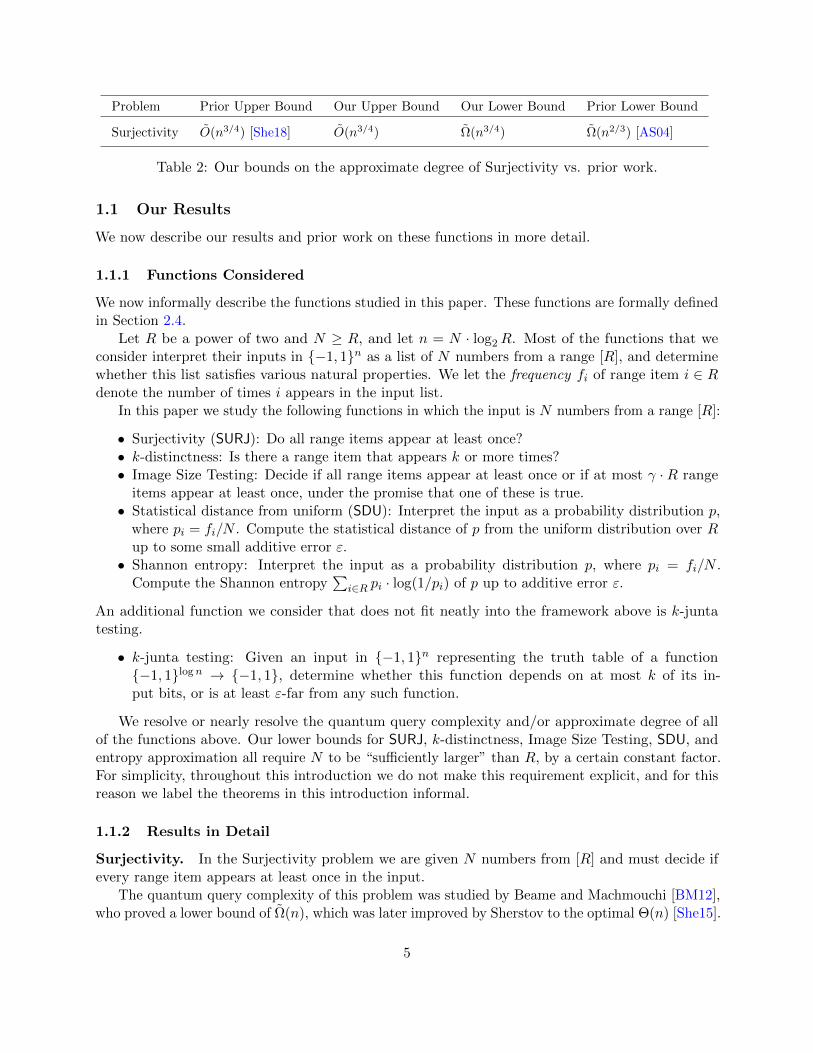
• Surjectivity: The approximate degree of the Surjectivity function is Ω(n3/4). The bestprior lower bound was Ω(n2/3). Our result matches an upper bound of O(n3/4) due toSherstov (STOC 2018), which we reprove using different techniques. The quantum querycomplexity of this function is known to be Θ(n) (Beame and Machmouchi, Quantum Inf.Comput. 2012 and Sherstov, FOCS 2015).
Our upper bound for Surjectivity introduces new techniques for approximating Booleanfunctions by low-degree polynomials. Our lower bounds are proved by significantly refiningtechniques recently introduced by Bun and Thaler (FOCS 2017).
1
arX
iv:1
710.
0907
9v2
[qu
ant-
ph]
25
May
201
8

Contents
1 Introduction 31.1 Our Results . . . . . . . . . . . . . . . . . . . . . . . . . . . . . . . . . . . . . . . . . 51.2 Prior Work on Lower Bounding Approximate Degree . . . . . . . . . . . . . . . . . . 81.3 Our Techniques . . . . . . . . . . . . . . . . . . . . . . . . . . . . . . . . . . . . . . . 91.4 Outline for the Rest of the Paper . . . . . . . . . . . . . . . . . . . . . . . . . . . . . 12
2 Preliminaries 122.1 Notation . . . . . . . . . . . . . . . . . . . . . . . . . . . . . . . . . . . . . . . . . . . 122.2 Two Variants of Approximate Degree and Their Dual Formulations . . . . . . . . . . 122.3 Basic Facts about Polynomial Approximations . . . . . . . . . . . . . . . . . . . . . 142.4 Functions of Interest . . . . . . . . . . . . . . . . . . . . . . . . . . . . . . . . . . . . 142.5 Connecting Symmetric Properties and Block Composed Functions . . . . . . . . . . 172.6 The Dual Block Method . . . . . . . . . . . . . . . . . . . . . . . . . . . . . . . . . . 182.7 A Refinement of a Technical Lemma from Prior Work . . . . . . . . . . . . . . . . . 19
3 Upper Bound for Surjectivity 193.1 Notation . . . . . . . . . . . . . . . . . . . . . . . . . . . . . . . . . . . . . . . . . . . 203.2 Warmup: Approximating NOR . . . . . . . . . . . . . . . . . . . . . . . . . . . . . . 203.3 Informal Terminology: Polynomials as Algorithms . . . . . . . . . . . . . . . . . . . 223.4 Approximating Surjectivity . . . . . . . . . . . . . . . . . . . . . . . . . . . . . . . . 22
4 Lower Bound for Surjectivity 314.1 Step 1: A Dual Witness for ORN . . . . . . . . . . . . . . . . . . . . . . . . . . . . . 324.2 Step 2: Constructing a Preliminary Dual Witness for ANDR ORN . . . . . . . . . . 354.3 Step 3: Constructing the Final Dual Witness . . . . . . . . . . . . . . . . . . . . . . 35
5 Lower Bound For k-Distinctness 365.1 Step 1: A Dual Witness for THRkN . . . . . . . . . . . . . . . . . . . . . . . . . . . . 375.2 Step 2: A Preliminary Dual Witness for ORR THRkN . . . . . . . . . . . . . . . . . 415.3 Step 3: Completing the Construction . . . . . . . . . . . . . . . . . . . . . . . . . . . 43
6 Lower Bound for Image Size Testing and Its Implications 446.1 Image Size Testing . . . . . . . . . . . . . . . . . . . . . . . . . . . . . . . . . . . . . 446.2 Lower Bound for Junta Testing . . . . . . . . . . . . . . . . . . . . . . . . . . . . . . 476.3 Lower Bound for SDU . . . . . . . . . . . . . . . . . . . . . . . . . . . . . . . . . . . 476.4 Lower Bound for Entropy Comparison and Approximation . . . . . . . . . . . . . . . 48
7 Conclusion and Open Questions 497.1 Additional Consequences: Approximate Degree Lower Bounds for DNFs and AC0 . . 497.2 Open Problems . . . . . . . . . . . . . . . . . . . . . . . . . . . . . . . . . . . . . . . 49
References 50
A Proof of Proposition 31 57A.1 Proof of Lemma 67 . . . . . . . . . . . . . . . . . . . . . . . . . . . . . . . . . . . . . 60
B Other Missing Proofs 62B.1 Refined Amplification Lemmas . . . . . . . . . . . . . . . . . . . . . . . . . . . . . . 62B.2 Correlation Calculation for GapANDγR ORN . . . . . . . . . . . . . . . . . . . . . . 66
2

1 Introduction
Approximate degree. The approximate degree of a Boolean function f : −1, 1n → −1, 1,denoted deg(f), is the least degree of a real polynomial p such that |p(x) − f(x)| ≤ 1/3 for allx ∈ −1, 1n. Approximate degree is a basic measure of the complexity of a Boolean function, andhas diverse applications throughout theoretical computer science.
Upper bounds on approximate degree are at the heart of the most powerful known learningalgorithms in a number of models [KS04,KS06,KKMS08,STT12,ACR+10,KT14,OS10], algorithmicapproximations for the inclusion-exclusion principle [KLS96,She09a], and algorithms for differentiallyprivate data release [TUV12,CTUW14]. A recent line of work [Tal14,Tal17] has used approximatedegree upper bounds to show new lower bounds on the formula and graph complexity of explicitfunctions.
Lower bounds on approximate degree have enabled progress in several areas of complexitytheory, including communication complexity [She11,BVdW07,She12,GS10,She13b,RY15,DPV09,CA08,DP08,She08], circuit complexity [MP69,She09b], oracle separations [Bei94,BCH+17], andsecret-sharing [BIVW16]. Most importantly for this paper, approximate degree lower bounds havebeen critical in shaping our understanding of quantum query complexity [BBC+01,Aar12,AS04],
In spite of the importance of approximate degree, major gaps remain in our understanding.In particular, the approximate degrees of many basic functions are still unknown. Our goal inthis paper is to resolve the approximate degrees of many natural functions which had previouslywithstood characterization.
Quantum query complexity. While resolving the approximate degree of basic functions ofinterest is a test of our understanding of approximate degree, it is also motivated by the study ofquantum algorithms. In the quantum query model, a quantum algorithm is given query access tothe bits of an input x, and the goal is to compute some function f of x while minimizing the numberof queried bits. Quantum query complexity captures much of the power of quantum computing,and most quantum algorithms were discovered in or can easily be described in the query setting.
Approximate degree was one of the first general lower bound techniques for quantum querycomplexity. In 1998, Beals et al. [BBC+01] observed that the bounded-error quantum querycomplexity of a function f is lower bounded by (one half times) the approximate degree of f . Sincepolynomials are sometimes easier to understand than quantum algorithms, this observation led toa number of new lower bounds on quantum query complexity. This method of proving quantumquery lower bounds is called the polynomial method.
After several significant quantum query lower bounds were proved via the polynomial method(including the work of Aaronson and Shi [AS04], who proved optimal lower bounds for the Collisionand Element Distinctness problems), the polynomial method took a back seat. Since then, thepositive-weights adversary method [Amb02,BSS03,LM04,Zha05] and the newer negative-weightsadversary method [HLS07,Rei11,LMR+11] have become the tools of choice for proving quantumquery lower bounds (with some notable exceptions, such as Zhandry’s recent tight lower bound forthe set equality problem [Zha15]). This leads us to our second goal for this work.
In this work, we seek to resolve several open problems in quantum query complexity usingapproximate degree as the lower bound technique. A distinct advantage of proving quantum querylower bounds with the polynomial method is that any such bound can be “lifted” via Sherstov’spattern matrix method [She11] to a quantum communication lower bound (even with unlimitedshared entanglement [LS09a]); such a result is not known for any other quantum query lower bound
3

Problem Best Prior Upper Bound Our Lower Bound Best Prior Lower Bound
k-distinctness O(n3/4−1/(2k+2−4)) [Bel12a] Ω(n3/4−1/(2k)) Ω(n2/3) [AS04]
Image Size Testing O(√n log n) [ABRdW16] Ω(
√n) Ω(n1/3) [ABRdW16]
k-junta Testing O(√k log k) [ABRdW16] Ω(
√k) Ω(k1/3) [ABRdW16]
SDU O(√n) [BHH11] Ω(
√n) Ω(n1/3) [BHH11,AS04]
Shannon Entropy O(√n) [BHH11,LW17] Ω(
√n) Ω(n1/3) [LW17]
Table 1: Our lower bounds on quantum query complexity and approximate degree vs. prior work.
technique. More generally, using approximate degree as a lower bound technique for quantumquery complexity has other advantages, such as the ability to show lower bounds for zero-error andsmall-error quantum algorithms [BCdWZ99], unbounded-error quantum algorithms [BBC+01], andtime-space tradeoffs [KSdW07].
Quantum query complexity and approximate degree. In this work we illustrate the powerof the polynomial method by proving optimal or nearly optimal bounds on several functions studiedin the quantum computing community. These results are summarized in Table 1, and definitions ofthe problems considered can be found in Section 1.1. Since the upper bounds for these functionswere shown using quantum algorithms, our results resolve both the quantum query complexity andapproximate degree of these functions.
For most of the functions studied in this paper, the positive-weights adversary bound provablycannot show optimal lower bounds due to the certificate complexity barrier [Zha05, SS06] and theproperty testing barrier [HLS07]. While these barriers do not apply to the negative-weights variant(which is actually capable for proving tight quantum query lower bounds for all functions [Rei11,LMR+11]), the negative-weights adversary method is often challenging to apply to specific problems,and the problems we consider have withstood characterization for a long time.
For the functions presented in Table 1, the approximate degree and quantum query complexityare essentially the same. This is not the case for the Surjectivity function, which has played animportant role in the literature on approximate degree and quantum query complexity. Specifically,Beame and Machmouchi [BM12] showed that Surjectivity has quantum query complexity Θ(n). Onthe other hand, Sherstov recently showed that Surjectivity has approximate degree O(n3/4) [She18].Surjectivity is the only known example of a “natural” function separating approximate degree fromquantum query complexity; prior examples of such functions [Amb03,ABK16] were contrived, and(unlike Surjectivity) specifically constructed to separate the two measures.
Our final result gives a full characterization of the approximate degree of Surjectivity. We provea new lower bound of Ω(n3/4), which matches Sherstov’s upper bound up to logarithmic factors. Wealso give a new construction of an approximating polynomial of degree O(n3/4), using very differenttechniques than [She18]. We believe that our proof of this O(n3/4) upper bound is of independentinterest. In particular, our lower bound proof for Surjectivity is specifically tailored to showingoptimality of our upper bound construction, in a sense that can be made formal via complementaryslackness. We are optimistic that our approximation techniques will be useful for showing additionaltight approximate degree bounds in the future.
4
Problem Prior Upper Bound Our Upper Bound Our Lower Bound Prior Lower Bound
Surjectivity O(n3/4) [She18] O(n3/4) Ω(n3/4) Ω(n2/3) [AS04]
Table 2: Our bounds on the approximate degree of Surjectivity vs. prior work.
1.1 Our Results
We now describe our results and prior work on these functions in more detail.
1.1.1 Functions Considered
We now informally describe the functions studied in this paper. These functions are formally definedin Section 2.4.
Let R be a power of two and N ≥ R, and let n = N · log2R. Most of the functions that weconsider interpret their inputs in −1, 1n as a list of N numbers from a range [R], and determinewhether this list satisfies various natural properties. We let the frequency fi of range item i ∈ Rdenote the number of times i appears in the input list.
In this paper we study the following functions in which the input is N numbers from a range [R]:
• Surjectivity (SURJ): Do all range items appear at least once?• k-distinctness: Is there a range item that appears k or more times?• Image Size Testing: Decide if all range items appear at least once or if at most γ ·R range
items appear at least once, under the promise that one of these is true.• Statistical distance from uniform (SDU): Interpret the input as a probability distribution p,
where pi = fi/N . Compute the statistical distance of p from the uniform distribution over Rup to some small additive error ε.• Shannon entropy: Interpret the input as a probability distribution p, where pi = fi/N .
Compute the Shannon entropy∑
i∈R pi · log(1/pi) of p up to additive error ε.
An additional function we consider that does not fit neatly into the framework above is k-juntatesting.
• k-junta testing: Given an input in −1, 1n representing the truth table of a function−1, 1logn → −1, 1, determine whether this function depends on at most k of its in-put bits, or is at least ε-far from any such function.
We resolve or nearly resolve the quantum query complexity and/or approximate degree of allof the functions above. Our lower bounds for SURJ, k-distinctness, Image Size Testing, SDU, andentropy approximation all require N to be “sufficiently larger” than R, by a certain constant factor.For simplicity, throughout this introduction we do not make this requirement explicit, and for thisreason we label the theorems in this introduction informal.
1.1.2 Results in Detail
Surjectivity. In the Surjectivity problem we are given N numbers from [R] and must decide ifevery range item appears at least once in the input.
The quantum query complexity of this problem was studied by Beame and Machmouchi [BM12],who proved a lower bound of Ω(n), which was later improved by Sherstov to the optimal Θ(n) [She15].
5

Beame and Machmouchi [BM12] explicitly leave open the question of characterizing the approximatedegree of Surjectivity. Recently, Sherstov [She18] showed an upper bound of O(n3/4) on theapproximate degree of this function. The best prior lower bound was Ω(n2/3) [AS04,BT17].
We give a completely different construction of an approximating polynomial for Surjectivitywith degree O(n3/4). We also prove a matching lower bound, which shows that the approximatedegree of the Surjectivity function is Θ(n3/4).
Theorem 1 (Informal). The approximate degree of SURJ is Θ(n3/4).
k-distinctness. In this problem, we are given N numbers in [R] and must decide if any rangeitem appears at least k times in the list (i.e., is there an i ∈ [R] with fi ≥ k?). This generalizes thewell-studied Element Distinctness problem, which is the same as 2-distinctness.
Ambainis [Amb07] first used quantum walks to give an O(nk/(k+1)) upper bound on the quantumquery complexity of any problem with certificates of size k, including k-distinctness and k-sum.1
Later, Belovs introduced a beautiful new framework for designing quantum algorithms [Bel12b]
and used it to improve the upper bound for k-distinctness to O(n3/4−1/(2k+2−4)) [Bel12a]. Severalsubsequent works have used Belovs’ k-distinctness algorithm as a black-box subroutine for solvingmore complicated problems (e.g., [LW17,Mon16]).
As for lower bounds, Aaronson and Shi [AS04] established an Ω(n2/3) lower bound on theapproximate degree of k-distinctness for any k ≥ 2. Belovs and Spalek used the adversary methodto prove a lower bound of Ω(nk/(k+1)) on the quantum query complexity of k-sum, showing thatAmbainis’ algorithm is tight for k-sum. They asked whether their techniques can prove an ω(n2/3)quantum query lower bound for k-distinctness. We achieve this goal, but using the polynomialmethod instead of the adversary method. Our main result is the following:
Theorem 2 (Informal). For any k ≥ 2, the approximate degree and quantum query complexity ofk-distinctness is Ω(n3/4−1/(2k)).
This is nearly tight for large k, as it approaches Belovs’ upper bound of O(n3/4−1/(2k+2−4)).Note that both bounds approach Θ(n3/4) as k →∞. It remains an intriguing open question to close
the gap between n3/4−1/(2k+2−4) and n3/4−1/(2k), especially for small values of k ≥ 3.Our k-distinctness lower bound also implies an Ω(n3/4−1/(2k)) lower bound on the quantum
query complexity of approximating the maximum frequency, F∞, of any element up to relative errorless than 1/k [Mon16], improving over the previous best bound of Ω(n2/3).
Image Size Testing. In this problem, we are given N numbers in [R] and γ > 0, and must decideif every range item appears at least once or if at most γ ·R range items appear at least once. Weshow for any γ > 0, the problem has approximate degree and quantum query complexity Ω(
√n).
This holds as long as N = c ·R for a certain constant c > 0.
Theorem 3 (Informal). The approximate degree and quantum query complexity of Image SizeTesting is Ω(
√n).
This lower bound is tight, matching a quantum algorithm of Ambainis, Belovs, Regev, and deWolf [ABRdW16], and resolves a conjecture from their work. The previous best lower bound wasΩ(n1/3) [ABRdW16] obtained via reduction to the Collision lower bound [AS04]. The classicalquery complexity of this problem is Θ(n/ log n) [VV11].
1In the k-sum problem, we are given N numbers in [R] and asked to decide if any k of them sum to 0 (mod R).
6

The version of image size testing we define is actually a special case of the one studied in[ABRdW16]. The version we define is solvable via the following simple algorithm making O(
√n)
queries: pick a random range item, and Grover search for an instance of that range item. Thefact that our lower bound holds even for this special case of the problem considered in prior worksobviously only makes our lower bound stronger.
This lower bound also serves as a starting point to establish the next three lower bounds.
k-junta Testing. In this problem, we are given the truth table of a Boolean function and have todetermine if the function depends on at most k variables or if it is ε-far from any such function.
The best classical algorithm for this problem uses O(k log k+ k/ε) queries [Bla09]. The problemwas first studied in the quantum setting by Atıcı and Servedio [AS07], who gave a quantum algorithmmaking O(k/ε) queries. This was later improved by Ambainis et al. [ABRdW16] to O(
√k/ε). They
also proved a lower bound of Ω(k1/3). Via a connection established by Ambainis et al., our imagesize testing lower bound implies a Ω(
√k) lower bound on the approximate degree and quantum
query complexity of k-junta testing (for some ε = Ω(1)).
Theorem 4 (Informal). The approximate degree and quantum query complexity of k-junta testingis Ω(
√k).
This matches the upper bound of [ABRdW16], resolving the main open question from theirwork.
Statistical Distance From Uniform (SDU). In this problem, we are given N numbers in [R],which we interpret as a probability distribution p, where pi = fi/N , the fraction of times i appears.The goal is to compute the statistical distance between p and the uniform distribution to error ε.
This problem was studied by Bravyi, Harrow, and Hassidim [BHH11], who gave an O(√n)-query
quantum algorithm approximating the statistical distance between two input distributions to additiveerror ε = Ω(1). We show that the approximate degree and quantum query complexity of this taskare Ω(
√n), even when one of the distributions is known to be the uniform distribution.
Theorem 5 (Informal). There is a constant c > 0 such that the approximate degree and quantumquery complexity of approximating the statistical distribution of a distribution over a range of size nfrom the uniform distribution over the same range to additive error c is is Ω(
√n).
This matches the upper bound of Bravyi et al. [BHH11] and answers the main question left openfrom that work. Note that the classical query complexity of this problem is Θ(n/ log n) [VV11].
Entropy Approximation. As in the previous problem, we interpret the input as a probabilitydistribution, and the goal is to compute its Shannon entropy to additive error ε. The classicalquery complexity of this problem is Θ(n/ log n) [VV11]. We show that, for some ε = Ω(1), theapproximate degree and quantum query complexity are Ω(
√n).
Theorem 6 (Informal). There is a constant c > 0 such that the approximate degree and quantumquery complexity of approximating the Shannon entropy of a distribution over a range of size n toadditive error c is is Ω(
√n).
This too is tight, answering a question of Li and Wu [LW17].
7

1.2 Prior Work on Lower Bounding Approximate Degree
A relatively new lower-bound technique for approximate degree called the method of dual polynomialsplays an essential role in our paper. This method of dual polynomials dates back to work ofSherstov [She13c] and Spalek [Spa08], though dual polynomials had been used earlier to resolvelongstanding questions in communication complexity [She11,SZ09,She09b,CA08,LS09b]. To prove alower bound for a function f via this method, one exhibits an explicit dual polynomial for f , whichis a dual solution to a certain linear program capturing the approximate degree of f .
A notable feature of the method of dual polynomials is that it is lossless, in the sense that itcan exhibit a tight lower bound on the approximate degree of any function f (though actuallyapplying the method to specific functions may be highly challenging). Prior to the method ofdual polynomials, the primary tool available for proving approximate degree lower bounds wassymmetrization, introduced by Minsky and Papert [MP69] in the 1960s. Although powerful,symmetrization is not a lossless technique.
Most prior work on the method of dual polynomials can be understood as establishing hardnessamplification results. Such results show how to take a function f that is “somewhat hard” toapproximate by low-degree polynomials, and turn f into a related function g that is much harderto approximate. Here, harder means either that g requires larger degree to approximate to thesame error as f , or that approximations to g of a given degree incur much larger error than doapproximations to f of the same degree.
Results for Block-Composed Functions. Until very recently, the method of dual polynomialshad been used exclusively to prove hardness amplification results for block-composed functions. Thatis, the harder function g would be obtained by block-composing f with another function h, i.e., g =h f . Here, a function g : −1, 1n·m → −1, 1 is the block-composition of h : −1, 1n → −1, 1and f : −1, 1m → −1, 1 if g interprets its input as a sequence of n blocks, applies f to eachblock, and then feeds the n outputs into h.
The method of dual polynomials turns out to be particularly suited to analyzing block-composedfunctions, as there are sophisticated ways of “combining” dual witnesses for h and f individuallyto give an effective dual witness for h f [She13c,SZ09,She13a,BT13,BT15,Tha16,She14,She15,BCH+17]. Prior work on analyzing block-composed functions has, for example, resolved theapproximate degree of the function f(x) = ∨ni=1 ∧mj=1 xij , known as the AND-OR tree, which had
been open for 19 years [BT13,She13a], established new lower bounds for AC0 under basic complexitymeasures including discrepancy [BT15, Tha16, She14, She15], sign-rank [BT16b], and thresholddegree [She15,She14], and resolved a number of open questions about the power of statistical zeroknowledge proofs [BCH+17].
Beyond Block-Composed Functions. While the aforementioned results led to considerableprogress in complexity theory, many basic questions require understanding the approximate degreeof non-block-composed functions. One prominent example with many applications is to exhibit anAC0 circuit over n variables with approximate degree Ω(n). Until very recently, the best result inthis direction was Aaronson and Shi’s well-known Ω(n2/3) lower bound on the approximate degree ofthe Element Distinctness function (which is equivalent to k-distinctness for k = 2) [AS04]. However,Bun and Thaler [BT17] recently achieved a near-resolution of this problem by proving the followingtheorem.
Theorem 7 (Bun and Thaler [BT17]). For any constant δ > 0, there is an AC0 circuit withapproximate degree Ω(n1−δ).
8

The reason that Theorem 7 required moving beyond block-composed functions is the following resultof Sherstov [She13d].
Theorem 8 (Sherstov). For any Boolean functions f and h, deg(h f) = O(
deg(h) · deg(f))
.
Theorem 8 implies that the approximate degree of h f (viewed as a function of its input size) isnever higher than the approximate degree of f or h individually (viewed as a function of their inputsizes). For example, if f and h are both functions on n inputs, and both have approximate degree
O(n1/2), then h f has N := n2 inputs, and by Theorem 8, deg(h f) = O(n1/2 · n1/2) = O(N1/2).This means that block-composing multiple AC0 functions does not result in a function of higher
approximate degree (as a function of its input size) than that of the individual functions. Bun andThaler [BT17] overcome this hurdle by introducing a way of analyzing functions that cannot bewritten as a block-composition of simpler functions.
Bun and Thaler’s techniques set the stage to resolve the approximate degree of many basicfunctions using the method of dual polynomials. However, they were not refined enough to accomplishthis on their own. Our lower bounds in this paper are obtained by refining and extending themethods of [BT17].
1.3 Our Techniques
In order to describe our techniques, it is helpful to explain the process by which we discovered thetight Θ(n3/4) lower and upper bounds for Surjectivity (cf. Theorem 1). It has previously beenobserved [Tha16,BT13,BT17] that optimal dual polynomials for a function f tend to be tailored(in a sense that can be made precise via complementary slackness) to showing optimality of somespecific approximation technique for f . Hence, constructing a dual polynomial for f can provide astrong hint as to how to construct an optimal approximation for f , and vice versa.
Upper Bound for Surjectivity. In [BT17], Bun and Thaler constructed a dual polynomialwitnessing a suboptimal bound of Ω(n2/3) for SURJ. Even though this dual polynomial is suboptimal,it still provided a major clue as to what an optimal approximation for SURJ should look like: itcuriously ignored all inputs failing to satisfy the following condition.
Condition 1. Every range item has frequency at most T , for a specific threshold T = O(N1/3) N .
This suggested that an optimal approximation for SURJ should treat inputs satisfying Condition 1differently than other inputs, leading us to the following multi-phase construction (for clarity andbrevity, this overview is simplified). The first phase constructs a polynomial p of degree O(n3/4)approximating SURJ on all inputs satisfying Condition 1. However, p may be exponentially large onother inputs. The second phase constructs a polynomial q of degree O(n3/4) that is exponentiallysmall on inputs x that do not satisfy Condition 1 (in particular, q(x) 1/p(x) for such x), and isclose to 1 otherwise. The product p · q still approximates SURJ on inputs satisfying Condition 1,and is exponentially small on all other inputs. Notice that deg(p · q) ≤ deg(p) + deg(q) = O(n3/4).Combining the above with an additional averaging step (the details of which we omit from thisintroduction) yields an approximation to SURJ that is accurate on all inputs.
9

Lower Bound for Surjectivity. With the O(n3/4) upper bound in hand, we were able to identifythe fundamental bottleneck preventing further improvement of the upper bound. This suggesteda way to refine the techniques of [BT17] to prove a matching lower bound. Once the tight lowerbound for SURJ was established, we were able to identify additional refinements to analyze theother functions that we consider. We now describe this in more detail.
Bun and Thaler’s [BT17] (suboptimal) lower bound analysis for SURJ proceeds in two stages.In the first stage, proving a lower bound for SURJ (on N input list items and R range items) isreduced to the problem of proving a lower bound for the block-composed function ANDR ORN ,2
under the promise that the input has Hamming weight at most N .3 In this paper, we use this stageof their analysis unmodified.
The second stage proves an Ω(R2/3) lower bound for the latter problem by leveraging much ofthe machinery developed to analyze the approximate degree of block-composed functions [BT13,She13a,RS10]. To describe this machinery, we require the following notion. A dual polynomial that
witnesses the fact that degε(fn) ≥ d is a function ψ : −1, 1n → −1, 1 satisfying three properties:
•∑
x∈−1,1n ψ(x) · f(x) > ε. If ψ satisfies this condition, it is said to be well-correlated with f .
•∑
x∈−1,1n |ψ(x)| = 1. If ψ satisfies this condition, it is said to have `1-norm equal to 1.
• For all polynomials p : −1, 1n → R of degree less than d, we have∑
x∈−1,1n p(x) ·ψ(x) = 0.If ψ satisfies this condition, it is said to have pure high degree at least d.
In more detail, the second stage of the analysis from [BT17] itself proceeds in two steps.First, the authors consider a dual witness ψ for the high approximate degree of ANDR ORNthat was constructed in prior work [BT13]. ψ is constructed by taking dual witnesses φ and γfor the high approximate degrees of ANDR and ORN individually, and “combining” them in aspecific way [SZ09,She13c,Lee09] to obtain a dual witness for the high approximate degree of theirblock-composition ANDR ORN .
Unfortunately, ψ only witnesses a lower bound for ANDR ORN without the promise that theHamming weight of the input is at most N . To address this issue, it is enough to “post-process” ψso that it no longer “exploits” any inputs of Hamming weight larger than N (formally, ψ(x) shouldequal zero for any inputs in −1, 1R·N of Hamming weight more than N). The authors accomplishthis by observing that ψ “almost ignores” all such inputs (i.e., it places exponentially little totalmass on all such inputs), and hence it is possible to perturb ψ to make it completely ignore all suchinputs.
Key to this step is the fact that the “inner” dual witness γ for the high approximate degree ofthe ORN function satisfies a “Hamming weight decay” condition:
|γ(x)| ≤ 1/poly(|x|), (1)
for a suitable polynomial function.
2When it is not clear from context, we use subscripts to denote the number of variables on which a function isdefined.
3Note that a reduction the other direction is straightforward: to approximate SURJ, it suffices to approximateANDR ORN on inputs of Hamming weight exactly N . This is because SURJ can be expressed as an ANDR (overall range items r ∈ [R]) of the ORN (over all input bits i ∈ [N ]) of “Is input xi equal to r”? Each predicate of theform in quotes is computed exactly by a polynomial of degree logR, since it depends on only logR of the inputs, andexactly N of these predicates (one for each i ∈ [N ]) evaluate to TRUE.
10

To improve the lower bound for SURJ from Ω(n2/3) to the optimal Ω(n3/4), we observe that γin fact satisfies a much stronger decay condition: while the inverse-polynomial decay property ofEquation (1) is tight for small Hamming weights |x|, |γ(x)| actually decays exponentially quicklyonce |x| is larger than a certain threshold t. This observation is enough to obtain the tight Ω(n3/4)lower bound for SURJ.
For intuition, it is worth mentioning that a primal formulation of the dual decay conditionthat we exploit shows that any low-degree polynomial p that is an accurate approximation to ORNon low Hamming weight inputs requires large degree, even if |p(x)| is allowed to be exponentiallylarge for inputs of Hamming weight more than t.4 This is precisely the bottleneck that prevents usfrom improving our upper bound for SURJ to o(N3/4). In this sense, our dual witness is intuitivelytailored to showing optimality of the techniques used in our upper bound.
Other Lower Bounds. To obtain the lower bound for k-distinctness, the first stage of theanalysis of [BT17] reduces to a question about the approximate degree of the block composedfunction ORR THRkN , under the promise that the input has Hamming weight at most N . HereTHRkN : −1, 1N → −1, 1 denotes the function that evaluates to −1 if and only if the Hammingweight of its input is at least k. By constructing a suitable dual witness for THRkN , and combiningit with a dual witness for ORN via similar techniques as in our construction for SURJ, we are ableto prove our Ω(n3/4−1/(2k)) lower bound for k-distinctness. (This description glosses over severalsignificant technical issues that must be dealt with to ensure that the combined dual witness iswell-correlated with ORR THRkN ).5
Recall that our lower bounds for k-junta testing, SDU, and entropy approximation are derivedas consequences of our lower bound for image size testing. The connection between image sizetesting and junta testing was established by Ambainis et al. [ABRdW16]. The reason that theimage testing lower bound implies lower bounds for SDU is the following. Consider any distributionp over [R] such that all probabilities pi are integer multiples of 1/N for some N = O(R). Then ifp has full support, p is guaranteed to be somewhat close to uniform, while if p has small support,p must be very far from uniform. We obtain our lower bound for entropy approximation using asimple reduction from SDU due to Vadhan [Vad99].
To obtain our lower bound for Image Size Testing, we observe that the first stage of the analysisof [BT17] reduces to a question about the approximate degree of the block composed functionGapANDRORN , under the promise that the input has Hamming weight at most N . Here, GapANDRis the promise function that outputs −1 if all of its inputs equal −1, outputs +1 if fewer than γ ·Rof its inputs are −1, and is undefined otherwise.
Roughly speaking, we obtain the desired Ω(n1/2) lower bound by combining a dual witness forGapANDR ORN from prior work [BT15] with the same techniques as in our construction for SURJ.However, additional technical refinements to the analysis of [BT17] are required to obtain our results.
4We do not formally describe this primal formulation of the dual decay condition, because it is not necessary toprove any of the results in this paper.
5Specifically, our analysis requires the dual witness γ for THRkN to be very well-correlated with THRkN in a certainone-sided sense (roughly, we need the probability distribution |γ| to have the property that, conditioned on γ outputting
a negative value, the input to γ is in(THRkN
)−1(−1) with probability at least 1− 1/(3R)). This property was not
required in the analysis for SURJ, which is why our lower bound for SURJ is larger by a factor of n1/(2k) than our lowerbound for k-distinctness. This seemingly technical issue is at least partially intrinsic: a polynomial loss compared tothe Ω(n3/4) lower bound for SURJ is unavoidable, owing to Belovs’ n3/4−Ω(1) upper bound [Bel12a] for k-distinctness.
11
In particular, the analysis of [BT17] only provides a lower bound for SURJ if N = Ω(R · log2(R)).But in order to infer our lower bound for SDU and entropy approximation (as well as k-junta testingfor ε = Ω(1)), it is essential that the lower bound hold for N = O(R). This is because a distributionwith full support is guaranteed to be Ω(1)-close to uniform if all probabilities are integer multiples of1/N with N = O(R), but this is not the case otherwise. (Consider, e.g., a distribution that placesmass 1 − 1/ log2(R) on a single range item, and spreads out the remaining mass evenly over allother range items). Refining the methods of [BT17] to yield lower bounds even when N = O(R)requires a significantly more delicate analysis than in [BT17].
1.4 Outline for the Rest of the Paper
Section 2 covers preliminary definitions and lemmas. Section 3 presents the O(n3/4) upper bound forSURJ, while Section 4 presents the matching Ω(n3/4) lower bound. Section 5 gives the Ω(n3/4−1/(2k))lower bound for k-distinctness. Section 6 presents the lower bound for Image Size Testing, and itsimplications for junta testing, SDU, and Shannon entropy approximation. Section 7 concludes bybriefly describing some additional consequences of our results, as well as a number of open questionsand directions for future work.
2 Preliminaries
2.1 Notation
For a natural number N , let [N ] = 1, 2, . . . , N and [N ]0 = 0, 1, 2, . . . , N. All logarithms aretaken in base 2 unless otherwise noted.
We will frequently work with Boolean functions under the promise that their inputs have lowHamming weight. To this end, we introduce the following notation for the set of low-Hammingweight inputs.
Definition 9. For 1 ≤ T ≤ n, let Hn≤T denote the subset of −1, 1n consisting of all inputs
Hamming weight at most T . We use |x| to denote the Hamming weight of an input x ∈ −1, 1n,so Hn
≤T = x ∈ −1, 1n : |x| ≤ T.
2.2 Two Variants of Approximate Degree and Their Dual Formulations
There are two natural notions of approximate degree for promise problems (i.e., for functions definedon a strict subset X of −1, 1n). One notion requires an approximating polynomial p to be boundedin absolute value even on inputs in −1, 1n \ X . The other places no restrictions on p outsideof the promise X . In this work, we make use of both notions. Hence, we must introduce some(non-standard) notation to distinguish the two.
Definition 10 (Approximate Degree With Boundedness Outside of the Promise Required). Letε > 0 and X ⊆ −1, 1n. The ε-approximate degree of a Boolean function f : X → −1, 1, denoted
degε(f), is the least degree of a real polynomial p : X → R such that |p(x) − f(x)| ≤ ε for allx ∈ X and |p(x)| ≤ 1 + ε for all x ∈ −1, 1n \ X . We use the term approximate degree without
qualification to refer to deg(f) = deg1/3(f).
The following standard dual formulation of this first variant of approximate degree can be foundin, e.g., [BT16a].
12

Proposition 11. Let X ⊆ −1, 1n, and let f : X → −1, 1. Then degε(f) ≥ d if and only ifthere exists a function ψ : −1, 1n → R satisfying the following properties.∑
x∈Xψ(x) · f(x)−
∑x∈−1,1n\X
|ψ(x)| > ε, (2)
∑x∈−1,1n
|ψ(x)| = 1, and (3)
For every polynomial p : −1, 1n → R of degree less than d,∑
x∈−1,1np(x) · ψ(x) = 0. (4)
We will refer to functions ψ : −1, 1n → R as dual polynomials. We refer to∑
x∈−1,1n |ψ(x)|as the `1-norm of ψ, and denote this quantity by ‖ψ‖1. If ψ satisfies Equation (4), it is said to havepure high degree at least d.
Given a function ψ : −1, 1n → R, and a (possibly partial) function f : X → −1, 1, whereX ⊆ −1, 1n, we let 〈f, ψ〉 :=
∑x∈X f(x) · ψ(x) −
∑x∈−1,1n\X |ψ(x)|, and refer to this as the
correlation of f and ψ. So Condition (2) is equivalent to requiring ψ and f to have correlation greatthan ε.
Definition 12 (Approximate Degree With Unboundedness Permitted Outside of the Promise).Let ε > 0 and X be a finite set. The ε-unbounded approximate degree of a Boolean function
f : X → −1, 1, denoted ubdegε(f), is the least degree of a real polynomial p : X → R such that|p(x)− f(x)| ≤ ε for all x ∈ X (if X is a strict subset of a larger domain, then no constraints areplaced on p(x) for x 6∈ X ). We use the term unbounded approximate degree without qualification
to refer to ubdeg(f) = ubdeg1/3(f).
The following standard dual formulation of this second variant of approximate degree canbe found in, e.g., [She11]. A dual polynomial ψ : −1, 1n → −1, 1 witnessing the fact that
ubdegε(f) ≥ d is the same as a dual witness for degε(f) ≥ d, but with the additional requirementthat ψ(x) = 0 outside of X .
Proposition 13. Let X ⊆ −1, 1n, and let f : X → −1, 1. Then ubdegε(f) ≥ d if and only ifthere exists a function ψ : −1, 1n → R satisfying the following properties.
ψ(x) = 0 for all x 6∈ X , (5)∑x∈X
ψ(x) · f(x) > ε, (6)∑x∈−1,1n
|ψ(x)| = 1, and (7)
For every polynomial p : −1, 1n → R of degree less than d,∑
x∈−1,1np(x) · ψ(x) = 0. (8)
Observe that deg(f) and ubdeg(f) coincide for total functions f . To avoid notational clutter,
when referring to the approximate degree of total functions, we will use the shorter notation deg(f).
13

2.3 Basic Facts about Polynomial Approximations
The seminal work of Nisan and Szegedy [NS94] gave tight bounds on the approximate degree of theANDn and ORn functions.
Lemma 14. For any constant ε ∈ (0, 1), the functions AND and OR on n bits have ε-approximatedegree Θ(n1/2), and the same holds for their negations.
Approximate degree is invariant under negating the inputs or output of a function, and hencethe result for AND implies the result for NAND, OR, etc.
The following lemma, which forms the basis of the well-known symmetrization argument, is dueto Minsky and Papert [MP69].
Lemma 15. Let p : −1, 1n → −1, 1 be an arbitrary polynomial and let [n]0 denote the set0, 1, . . . , n. Then there is a univariate polynomial q : R→ R of degree at most deg(p) such that
q(t) =1(nt
) ∑x∈−1,1n : |x|=t
p(x)
for all t ∈ [n]0.
2.4 Functions of Interest
We give formal definitions of the Surjectivity, k-distinctness, SDU, and Shannon Entropy functionswe consider in this work, as well as several variations that will be helpful in proving our lowerbounds.
2.4.1 Surjectivity
Definition 16. For N ≥ R, define the function SURJN,R : [R]N → −1, 1 by SURJN,R(s1, . . . , sN ) =−1 iff for every j ∈ [R], there exists an i such that si = j.
When N and R are clear from context, we will often refer to the function SURJ without theexplicit dependence on these parameters. It will sometimes be convenient to think of the input toSURJN,R as a function mapping −1, 1n → −1, 1 rather than [R]N → −1, 1. When needed, weassume that R is a power of 2 and an element of [R] is encoded in binary using logR bits. In thiscase we will view Surjectivity as a function on n = N logR bits, i.e., SURJ : −1, 1n → −1, 1.
For technical reasons, when proving lower bounds, it will be more convenient to work with avariant of SURJ where the range [R] is augmented by a “dummy element” 0 that is simply ignored bythe function. That is, while any of the items s1, . . . , sN may take the dummy value 0, the presenceof a 0 in the input is not required for the input to be deemed surjective. We denote this variant ofSurjectivity by dSURJ. More formally:
Definition 17. For N ≥ R, define the function dSURJN,R : [R]N0 → −1, 1 by dSURJN,R(s1, . . . , sN ) =−1 iff for every j ∈ [R], there exists an i such that si = j.
The following simple reduction shows that a lower bound on the approximate degree of dSURJimplies a lower bound for SURJ itself.
14

Proposition 18. Let ε > 0 and N ≥ R. Then
degε(dSURJN,R) ≤ degε(SURJN+1,R+1) · log(R+ 1).
Proof. Let p : −1, 1(N+1)·log(R+1) → −1, 1 be a polynomial of degree d that ε-approximatesSURJN+1,R+1. We will use p to construct a polynomial of degree d that ε-approximates dSURJN,R.Recall that an input to dSURJN,R takes the form (s1, . . . , sN ) where each si is the binary represen-tation of a number in [R]0. Define the transformation T : [R]0 → [R+ 1] by
T (s) =
R+ 1 if s = 0
s otherwise.
Note that as a mapping between binary representations, the function T is exactly computed by avector of polynomials of degree at most log(R+ 1). For every (s1, . . . , sN ) ∈ [R]N0 , observe that
dSURJN,R(s1, . . . , sN ) = SURJN+1,R+1(T (s1), . . . , T (sN ), R+ 1).
Hence, the polynomial
p(T (s1), . . . , T (sN ), R+ 1)
is a polynomial of degree d · log(R+ 1) that ε-approximates dSURJN,R.
2.4.2 k-Distinctness
Definition 19. For integers k,N,R with k ≤ N , define the function DISTkN,R : [R]N → −1, 1 by
DISTkN,R(s1, . . . , sN ) = −1 iff there exist r ∈ [R] and distinct indices i1, . . . , ik such that si1 = · · · =sik = r.
As with Surjectivity, it will be convenient to work with a variant of k-distinctness where [R] isaugmented with a dummy item:
Definition 20. For integers k,N,R with k ≤ N , define the function dDISTkN,R : [R]N0 → −1, 1by dDISTkN,R(s1, . . . , sN ) = −1 iff there exist r ∈ [R] and distinct indices i1, . . . , ik such thatsi1 = · · · = sik = r.
For k ≥ 2, a lower bound on the approximate degree of dDISTk implies a lower bound on theapproximate degree of DISTk. The restriction that k ≥ 2 is essential, because the function DIST1
is the constant function that evaluates to TRUE on any input (since at least one range item mustalways have frequency at least one), whereas dDIST1 contains ORN as a subfunction, and hence hasapproximate degree at least Ω(
√N).
Proposition 21. Let ε > 0, N,R ∈ N, and k ≥ 2. Then
degε(dDISTkN,R) ≤ degε(DIST
kN,R+N ) · log(R+ 1).
Proof. The proof is similar to that of Proposition 18, but uses a slightly more involved reduction.Let p : −1, 12N ·log(R+N) → −1, 1 be a polynomial of degree d that ε-approximates DISTkN,R+N .
15

We will use p to construct a polynomial of degree d that ε-approximates dDISTkN,R. For eachi = 1, . . . , R, define a transformation Ti : [R]0 → [R+N ] by
Ti(s) =
R+ i if s = 0
s otherwise.
As a mapping between binary representations, the function T = (T1, . . . , TN ) is exactly computedby a vector of polynomials of degree at most log(R+ 1). For every (s1, . . . , sN ) ∈ [R]N0 , observe that
dDISTkN,R(s1, . . . , sN ) = DISTkN,R+N (T1(s1), . . . , TN (sN )).
Hence, the polynomial
p(T (s1), . . . , T (sN ))
is a polynomial of degree d · log(R+ 1) that ε-approximates dSURJN,R.
2.4.3 Image Size Testing
The Image Size Testing problem (IST for short) is defined as follows.
Definition 22. Given an input s = (s1, . . . , sN ) ∈ [R]N0 , and i ∈ [R], let fi = |j : sj = i|. Theimage size of s is the number of i ∈ [R] such that fi > 0. For 0 < γ < 1, define:
ISTγN,R(s1, . . . , sN ) =
−1 if the image size is R
1 if the image size is at most γ ·Rundefined otherwise.
Observe that the definition of IST ignores whether or not the range item 0 has positive frequency,just like the functions dSURJ and dDISTk. We choose to define IST in this manner to streamlineour analysis.
2.4.4 Statistical Distance from Uniform (SDU)
Given an input (s1, . . . , sN ) ∈ [R]N , and i ∈ [R], let fi = |j : sj = i|, and let p be the probabilitydistribution over [R] such that pi = fi/N . For N ≥ R and 0 < γ2 < γ1 < 1, define the partialfunction SDUγ1,γ2
N,R as follows.
Definition 23. Define
SDUγ1,γ2
N,R (s1, . . . , sN ) =
−1 if 1
2
∑Ri=1 |pi − 1/R| ≥ γ1
1 if 12
∑Ri=1 |pi − 1/R| ≤ γ2
undefined otherwise.
Above, 12
∑Ri=1 |pi − 1/R| is the statistical distance between p and the uniform distribution.
16

2.4.5 Entropy
Given a distribution p over [R], the Shannon entropy of p, denoted H(p), is defined to be∑i∈[R] pi log2(1/pi). Following Goldreich and Vadhan [GV11], we define a partial function GapCmprEntα,βN,R
capturing the problem of comparing the entropies of two distributions.The function GapCmprEntα,βN,R takes as input two vectors in [R]N and interprets each vector
i ∈ 1, 2 as a probability distribution pi over [R], with pi(j) = fi,j/N where fi,j is the frequency of
j in the ith vector. The function GapCmprEntα,βN,R evaluates to−1 if H(p1)−H(p2) ≤ β1 if H(p1)−H(p2) ≥ αundefined otherwise.
2.5 Connecting Symmetric Properties and Block Composed Functions
An important ingredient in [BT17] is the relationship between the approximate degree of a propertyof a list of numbers (such as SURJ) and the approximate degree of a simpler block composedfunction, defined as follows.
Definition 24. For functions f : Y n → Z and g : X → Y , define the block composition f g :Xn → Z by (f g)(x1, . . . , xn) = f(g(x1), . . . , g(xn)), for all x1, . . . , xn ∈ X.
Fix R,N ∈ N, let f : −1, 1R → −1, 1 and let g : −1, 1N → −1, 1. Suppose g is asymmetric function, in the sense that for any x ∈ −1, 1N and any permutation σ : [N ]→ [N ], wehave
g(x1, . . . , xN ) = g(xσ(1), . . . , xσ(N)).
Equivalently, the value of g on any input x depends only on its Hamming weight |x|.The functions f and g give rise to two functions. The first, which we denote by F prop : [R]N0 →
−1, 1, is a certain property of a list of numbers s1, . . . , sN ∈ [R]0. The second, which we denoteby F≤N : HN ·R
≤N → −1, 1, is the block composition of f and g restricted to inputs of Hammingweight at most N . Formally, these functions are defined as:
F prop(s1, . . . , sN ) = f(g(1[s1 = 1], . . . ,1[sN = 1]), . . . , g(1[s1 = R], . . . ,1[sN = R]))
F≤N (x1, . . . , xR) =
f(g(x1), . . . , g(xR)) if x1, . . . , xR ∈ −1, 1N , |x1|+ · · ·+ |xR| ≤ N.undefined otherwise.
The following proposition relates the approximate degrees of the two functions F prop and F≤N .
Theorem 25 (Bun and Thaler [BT17]). Let f : −1, 1R → −1, 1 be any function and letg : −1, 1N → −1, 1 be a symmetric function. Then for F prop and F≤N defined above, and forany ε > 0, we have
degε(Fprop) ≥ ubdegε(F
≤N ).
In the case where f = ANDR and g = ORN , the function F prop(s1, . . . , sN ) is the Surjectivityfunction augmented with a dummy item, dSURJN,R(s1, . . . , sN ). Hence,
17

Corollary 26. Let N,R ∈ N. Then for any ε > 0,
degε(dSURJN,R) ≥ ubdegε(F≤N )
where F≤N : HN ·R≤N → −1, 1 is the restriction of ANDR ORN to HN ·R
≤N .
Definition 27. For integers k,N with k ≤ N , define the function THRkN : −1, 1N → −1, 1 byTHRkN (x) = −1 iff |x| ≥ k.
If we let f = ORR and g = THRNk , then the function F prop is the dummy augmented k-distinctnessfunction dDISTkN,R.
Corollary 28. Let N,R ∈ N. Then for any ε > 0,
degε(dDISTkN,R) ≥ ubdegε(G
≤N )
where G≤N : HN ·R≤N → −1, 1 is the restriction of ORR THRN to HN ·R
≤N .
2.6 The Dual Block Method
This section collects definitions and preliminary results on the dual block method [SZ09,Lee09,She13c]for constructing dual witnesses for a block composed function F f by combining dual witnesses forF and f respectively.
Definition 29. Let Ψ : −1, 1M → R and ψ : −1, 1m → R be functions that are not identicallyzero. Let x = (x1, . . . , xM ) ∈ (−1, 1m)M . Define the dual block composition of Ψ and ψ, denotedΨ ? ψ : (−1, 1m)M → R, by
(Ψ ? ψ)(x1, . . . , xM ) = 2M ·Ψ(. . . , sgn (ψ(xi)) , . . . ) ·M∏i=1
|ψ(xi)|.
Proposition 30 ([She13c,BT17]). The dual block composition satisfies the following properties:
Preservation of `1-norm: If ‖Ψ‖1 = 1, ‖ψ‖1 = 1, and 〈ψ,1〉 = 0, then
‖Ψ ? ψ‖1 = 1. (9)
Multiplicativity of pure high degree: If 〈Ψ, P 〉 = 0 for every polynomial P : −1, 1M →−1, 1 of degree less than D, and 〈ψ, p〉 = 0 for every polynomial p : −1, 1m → −1, 1 of degreeless than d, then for every polynomial q : −1, 1m·M → −1, 1,
deg q < D · d =⇒ 〈Ψ ? ψ, q〉 = 0. (10)
Associativity : For every ζ : −1, 1mζ → R, ϕ : −1, 1mϕ → R, and ψ : −1, 1mψ → R, wehave
(ζ ? ϕ) ? ψ = ζ ? (ϕ ? ψ). (11)
18
2.7 A Refinement of a Technical Lemma from Prior Work
The following technical proposition refines techniques of Bun and Thaler [BT17]. This proposition isuseful for “zeroing out” the mass that a dual polynomial ξ places on inputs of high Hamming weight,if ξ is obtained via the dual-block method. The proof of the proposition is deferred to Appendix A.
Proposition 31. Let R ∈ N be sufficiently large, and let Φ : −1, 1R → R with ‖Φ‖1 = 1. ForM ≤ R, let ω : [M ]0 → R and parameters 1 ≤ α ≤ R2, β ∈ (4 ln2R/
√αR, 1) be such that
M∑t=0
ω(t) = 0, (12)
M∑t=0
|ω(t)| = 1, (13)
|ω(t)| ≤ α exp(−βt)/t2 ∀t = 1, 2, . . . ,M. (14)
Let N = d20√αeR, and define ψ : −1, 1N → R by ψ(x) = ω(|x|)/
(N|x|). If D < N is such that
For every polynomial p with deg p < D, we have 〈Φ ? ψ, p〉 = 0, (15)
then there exist ∆ ≥ β√αR/4 ln2R and a function ζ : (−1, 1N )R → R such that
For every polynomial p with deg p < minD,∆, we have 〈ζ, p〉 = 0, (16)
‖ζ − Φ ? ψ‖1 ≤2
9, (17)
‖ζ‖1 = 1, (18)
ζ is supported on HN ·R≤N . (19)
The key refinement of Proposition 31 relative to the analysis of Bun and Thaler is that Proposition31 applies when N = Θ(R) (assuming α = O(1)). In contrast, the techniques of Bun and Thalerrequired N = Ω(R · log2R). As indicated in Section 1.3, this refinement will be essential in obtainingour lower bounds for SDU, entropy approximation, and junta testing for constant proximityparameter.
3 Upper Bound for Surjectivity
The goal of this section is to prove that the approximate degree of the Surjectivity function(Definition 16) is O(N3/4).
Theorem 32. For any R ∈ N, we have deg(SURJN,R) = O(N3/4).
For the remainder of the section, we focus on proving Theorem 32 in the case that R = Θ(N).This is without loss of generality by the following argument. If R > N , then Surjectivity is identicallyfalse, and hence has (exact) degree 0. And if R = o(N), then we can reduce to the case R = Θ(N)as follows. Let N ′ = 2N and R′ = R+N ; clearly R′ = Θ(N). Given an input x to SURJN,R, obtainan input x′ to SURJN ′,R′ by appending range elements R+ 1, . . . , R+N to x. This construction
19

guarantees that SURJN,R(x) = SURJN ′,R′(x′). It follows that an approximation of degree O(N3/4)
for SURJN ′,R′ implies an approximation of the same degree for SURJN,R.
Section Outline. This section is structured as follows. Section 3.1 introduces some notation thatis specific to this section. Section 3.2 provides some intuition for the construction of the polynomialapproximation for Surjectivity using the simpler function NOR as a warmup example. Section 3.3introduces some terminology that is useful for providing intuitive descriptions of our final polynomialconstruction using the language of algorithms. Finally, in Section 3.4 we formally apply our strategyto Surjectivity in order to prove Theorem 32.
3.1 Notation
In this section, we make a few departures from the notation used in the introduction and later sectionsin order to more easily convey the algorithmic intuition behind our polynomial constructions. First,we will consider Boolean functions f : 0, 1n → 0, 1, where 1 corresponds to logical TRUE and 0corresponds to logical FALSE. For such a Boolean function, we say that a polynomial p : 0, 1n → Ris an ε-approximating polynomial for f if p(x) ∈ [0, ε] when f(x) = 0 and p(x) ∈ [1 − ε, 1] whenf(x) = 1. For such a polynomial p, it will be useful to think of p(x) as representing the probabilitythat a randomized or quantum algorithm accepts when run on input x.
By extension, throughout this section we will use degε(f) to denote the least degree of a real
polynomial p that ε-approximates f in the sense described above, and we will write deg(f) =
deg1/3(f). Given an input x ∈ 0, 1n, we will use |x| to denote its Hamming weight (i.e., |x| =∑i xi).
3.2 Warmup: Approximating NOR
To convey the intuition behind our polynomial construction for Surjectivity, we start by consideringa much simpler function as an illustrative example. Consider the negation of the OR function onn bits, NOR : 0, 1n → 0, 1. We will give a novel construction of an approximating polynomialfor NOR of degree O(
√n). Of course, this is not terribly interesting since it is already known that
deg(NOR) = Θ(√n) (cf. Lemma 14). But this construction highlights the main idea behind the
more involved constructions to follow.In many models of computation, such as deterministic or randomized query complexity, the
NOR function remains just as hard if we restrict to inputs with |x| = 0 or |x| = 1 (where |x| denotesthe Hamming weight of x ∈ 0, 1n). This is fairly intuitive, since distinguishing these two types ofinputs essentially requires finding a single 1 among n possible locations. The fact that these inputsrepresent the “hard case” is true for approximate degree as well: any polynomial that uniformlyapproximates NOR to error 1/3 on Hamming weights 0 and 1, and merely remains bounded in [0, 1]on the rest of the hypercube, has degree Ω(
√n) [NS94].
However, if we remove the boundedness constraint on inputs of Hamming weight larger than 1,then there is a polynomial of degree one that exactly equals the NOR function on Hamming weights0 and 1: namely, the polynomial 1−
∑i xi. That is, if we view NOR as a promise function mapping
Hn≤1 to −1, 1, then its approximate degree is Θ(n1/2), but its unbounded approximate degree isjust 1.
More generally, suppose that we only want the polynomial to approximate the NOR function onall inputs of Hamming weight up to T ≤ n, and we place no restrictions on the polynomial when
20
evaluated at inputs of Hamming weight larger than T . This can be achieved by a polynomial ofdegree O(
√T ) (see Lemma 34 for a proof).
Let us refer to the set of low-Hamming weight inputs as P, i.e.,
P = Hn≤T = x ∈ 0, 1n : 0 ≤ |x| ≤ T. (20)
The above discussion shows that we can construct a polynomial p of degree O(√T ) that tightly
approximates NOR on inputs x ∈ P, though |p(x)| may be exponentially large for x /∈ P. On theother hand, distinguishing inputs with |x| = 0 from inputs with x /∈ P also seems “easy”. Forexample, a randomized algorithm that simply samples Θ(n/T ) bits and declares |x| = 0 if and onlyif it does not see a 1 is correct with high probability. Analogously, we can construct a low-degreepolynomial q which distinguishes between |x| = 0 or x /∈ P (and is bounded in [0, 1] for all inputs in0, 1n): it is not hard to show (via an explicit construction involving Chebyshev polynomials, or byappeal to a quantum algorithm called quantum counting [BHT98]) that there exists a polynomial qof degree O(
√n/T ) that accomplishes this.
To summarize the above discussion, we can construct polynomials p and q, of degree O(√T )
and O(√n/T ) respectively, with the following properties:
p(x) ∈
[9/10, 1] if |x| = 0
[0, 1/10] if 1 ≤ |x| ≤ TR if x /∈ P
q(x) ∈
[9/10, 1] if |x| = 0
[0, 1] if 1 ≤ |x| ≤ T[0, 1/10] if x /∈ P
(21)
Now consider the polynomial p(x) · q(x). This polynomial approximates NOR on |x| = 0, sinceits value is in [0.81, 1]. It also approximates NOR on 1 ≤ |x| ≤ T , since its value is in [0, 1/10].However, when x /∈ P , although q(x) is small, we cannot ensure that the product p(x) · q(x) is small,since we have no control over p(x) for such x.
To fix this, we will construct a new polynomial q that behaves like q for x ∈ P and is extremelysmall when x /∈ P (in particular 0 ≤ q(x) 1/|p(x)| for such x). To understand how small we needq to be, we need to determine just how large p(x) can be on inputs with x /∈ P.
To understand the behavior of p(x) outside of P, we can either analyze the behavior of anexplicit polynomial of our choice for the NOR function or we can appeal to a general result aboutthe growth of polynomials that are bounded in a region (see Lemma 34). In either case, we get thatthere exists an upper bound M = exp(O(
√T log n)) such that for all x /∈ P, |p(x)| ≤M .
This leads us to design a new polynomial q, which has the same behavior as q for all x ∈ P , but isat most 1/(3M) when x /∈ P . We can construct the polynomial q from q by applying standard errorreduction to reduce the approximation error of q to ε = 1/(3M), which increases its the degree by amultiplicative factor of O(log(3M)) = O(
√T log n). Thus, deg(q) = O(
√n/T ·
√T log n) = O(
√n).
In summary, we have now constructed polynomials p and q with the following behavior:
p(x) ∈
[9/10, 1] if |x| = 0
[0, 1/10] if 1 ≤ |x| ≤ T[0,M ] if x /∈ P
q(x) ∈
[1− 1/(3M), 1] if |x| = 0
[0, 1] if 1 ≤ |x| ≤ T[0, 1/(3M)] if x /∈ P
(22)
Caricatures of these polynomials are depicted in Figure 1 and Figure 2. It is now easy to seethat the product r(x) = p(x) · q(x) is a (1/3)-error approximation to NOR for all x ∈ 0, 1n. Thedegree of the constructed polynomial is deg(r) ≤ deg(p) + deg(q) = O(
√T +√n) = O(
√n).
Thus our constructed polynomial, r, has degree O(√n) and approximates NOR to error 1/3,
which is optimal by Lemma 14.
21

Figure 1: Caricature of the polynomial p(x) Figure 2: Caricature of the polynomial q(x)
3.3 Informal Terminology: Polynomials as Algorithms
Before moving on to Surjectivity, we briefly introduce some terminology that will allow us convey theintuition of more involved constructions by reasoning about polynomials as if they were algorithms.
Consider three Boolean functions p1 : 0, 1n → 0, 1, p2 : 0, 1n → 0, 1 and p3 : 0, 1n →0, 1, and suppose there are deterministic algorithms A1, A2, and A3 that compute these Booleanfunctions exactly. Now it makes sense to say “run algorithm A1 in input x; if it accepts then outputA2(x), and if it rejects, then output A3(x).” The Boolean function computed by this is A2(x) ifA1(x) = 1 and A3(x) if A1(x) = 0. Observe that the following polynomial composition of p1, p2, p3
computes the same Boolean function: p1(x)p2(x) + (1− p1(x))p3(x).We would like to use this terminology to discuss combining polynomials more generally. For
polynomials p that approximate Boolean functions by outputting a value in [0, 1] on any input x, wecan imagine p(x) as representing the probability that a randomized (or quantum) algorithm acceptson input x, and the same interpretation goes through. We will also use the same terminology forpolynomials that output values greater than 1, in which case we cannot interpret the output as aprobability, but expressions like p1(x)p2(x) + (1− p1(x))p3(x) still make sense.
For example, in the previous section we had two polynomials p and q and we constructed thepolynomial r(x) = p(x) · q(x) by multiplying the two polynomials together. Another way to think ofthis is that r is the polynomial obtained when we “run” the polynomial q and output p if it acceptsand output 0 if it rejects. This yields the polynomial q(x)p(x) + (1− q(x)) · 0 = q(x)p(x). We wouldlike to informally describe polynomial constructions using this language, which will be especiallyuseful when the constructions become more involved. So for example, we would informally describethe polynomial we constructed for the NOR function as follows (Polynomial 1):
Polynomial 1 An informal description of the polynomial approximation for NOR
1: Using q, check if |x| > T (with exponentially small probability of error if indeed |x| > T ). If so,halt and output 0.
2: Using p, compute NOR under the promise that 0 ≤ |x| ≤ T and output the result.
3.4 Approximating Surjectivity
We now construct a polynomial that approximates Surjectivity using the strategy described above.Recall that SURJ : [R]n → 0, 1 is defined by SURJ(x1, . . . , xn) = 1 if and only if for all r ∈ [R]
22

there exists an i ∈ [N ] such that xi = r.In this section, we will use the notation
#r(x) = |i ∈ [N ] : xi = r| (23)
to denote the number of times the range element r appears in the input x. Note that the Surjectivityfunction evaluates to 1 if and only if #r(x) ≥ 1 for all r ∈ [R].
Finally, we will also need to consider a generalized version of Surjectivity, R-Surjectivity forsome set R ⊆ [R], which we denote SURJR. As with Surjectivity,
SURJR : [R]N → 0, 1, (24)
and SURJR(x1, . . . , xn) = 1 if and only if for all r ∈ R there exists an i ∈ [N ] such that xi = r.In other words, SURJR(x) = 1 if and only if for all r ∈ R we have #r(x) ≥ 1. Note that
SURJ[R] = SURJ. Our construction will actually show more generally that deg(SURJR) = O(N3/4)for all R ⊆ [R].
3.4.1 Approximating Surjectivity on the Hard Inputs
To implement the strategy described in Section 3.2 in the context of Surjectivity, we first choose aset P of inputs that we consider to be “hard”. Since Surjectivity can be phrased as asking whetherall range items appear at least once in the input, it is natural to consider the hard inputs to bethose that have few occurrences of each range item. Intuitively, this is because on such inputs,evidence that any given range item r appears at least once in the input is hard to find.
To this end, we define P as the set of inputs for which every range item appears at most Ttimes, for a parameter T to be chosen later:
P = x : ∀r ∈ [R], #r(x) ≤ T. (25)
More generally, when we consider R-Surjectivity, we denote the set of hard inputs PR and define itas
PR = x : ∀r ∈ R, #r(x) ≤ T. (26)
In this section, we will construct a polynomial pR that approximates SURJR on PR to boundederror, but may be exponentially large outside of PR. The value of T in the definition of PR will bechosen later; for now we only assume that our choice will satisfy T = NΘ(1), which simplifies someexpressions since we have log T = Θ(logN).
Overview of the Construction of pR. To construct a polynomial that works on the hard inputs,PR, we first express SURJR as
SURJR(x) =∧r∈R
∨i∈[N ]
1[xi = r], (27)
where 1[xi = r] is the indicator function that takes value 1 when xi = r and 0 otherwise. Observethat for any fixed r ∈ R, the function 1[xi = r] depends on only logR bits of x and hence can beexactly computed by a polynomial of degree at most logR.
23

Since our goal in this section is to construct a polynomial pR that approximates SURJR on allinputs in PR and may be exponentially large outside of PR, we can assume that each inner OR gatein Equation (27) is fed an input of Hamming weight at most T . Hence, our approach will be to first
construct a low-degree polynomial q that approximates AND|R| ORN for inputs in(HN≤T
)|R|. We
then obtain the polynomial pR that approximates SURJR at all inputs in PR by composing q withthe indicator functions 1[xi = r]i∈[N ],r∈R. Notice that the degree of pR is at most deg(q) · logR
To construct q, our approach is as follows. First, we construct a polynomial VT of degreeO(T 1/2 logN) that approximates ORN to error O(1/N) at all inputs of Hamming weight at mostT . (However, VT (x) may be as large as exp(T 1/2 logN) for inputs x of larger Hamming weight).Invoking Lemma 14, we let w be a polynomial of degree Θ(N1/2) that approximates ANDN to error1/20, and finally we define q := w VT . A simple and elegant analysis of Buhrman et al. [BNRdW07]
(cf. Lemma 35) allows us to argue that q indeed approximates AND|R| ORN on(HN≤T
)|R|.
Preliminary Lemmas. Before formally defining and analyzing pR, we record a few importantfacts about Chebyshev polynomials that will be useful throughout the remainder of this section.
Lemma 33 (Properties of Chebyshev Polynomials). Let d ∈ N.
(1) There exists a polynomial Td : R → R (the Chebyshev polynomial of degree d) such thatTd(x) ∈ [−1, 1] for all x ∈ [−1, 1] and Td(1 + µ) ≥ 1
2 exp(d√µ) for all µ ∈ (0, 1).
(2) For any polynomial p : R→ R of degree d with |p(x)| ≤ 1 for all x ∈ [−1, 1], we have that forany x with |x| > 1,
|p(x)| ≤ Td(x) ≤ (2|x|)d, (28)
where Td is the Chebyshev polynomial of degree d.
Proof. To establish property (1), we use the fact that for µ > 0, the value of the degree d Chebyshevpolynomial can be written [Che82, §3.2 Problem 8(f)] as
Td(1 + µ) = cosh(d arcosh(1 + µ))
≥ cosh(d√µ) for µ ≤ 1
≥ 1
2· exp(d
õ).
Property (2) appears as [Che82, 3.2 Problem 19].
We are now ready to establish the existence of a low-degree polynomial that approximates ORat all inputs of low Hamming weight.
Lemma 34 (Approximating OR on Inputs of Low Hamming Weight). Let ε ∈ (0, 1) and 1 ≤ T ≤ N .There is a polynomial VT,ε : 0, 1N → R of degree O(
√T log(1/ε)) such that
VT,ε(x) ∈
[0, ε] if |x| = 0
[1− ε, 1] if 1 ≤ |x| ≤ T[−a, a] for some a ∈ exp
(O(√
T · logN · log (1/ε)))
if |x| > T
. (29)
24

Proof. Choose d = O(√T log(1/ε)) so that M := Td(1 + 1/T ) + 1 ≥ 2/ε (as guaranteed by Property
1 of Lemma 33). Define VT,ε by the following affine transformation of Td:
VT,ε(x) =
(1− 1
M
)− 1
M· Td
(1 +
1
T− |x|
T
).
Then for |x| = 0, we have
VT,ε(x) =
(1− 1
M
)− 1
M· Td
(1 +
1
T
)= 0.
If 1 ≤ |x| ≤ T , then 1 + 1/T − |x|/T ∈ [−1, 1], so VT,ε(x) ∈ [1 − ε, 1]. Finally, if T + 1 ≤ |x| ≤ N ,then
|VT,ε(x)| ≤ 1 +1
M· Td(N/T ) ≤ exp(O(
√T · logN · log(1/ε)).
The following lemma shows that if p and q are approximating polynomials for Boolean functionsf and g, respectively, then the block composition p q approximates f g, with a blowup in errorthat is proportional to the number of variables over which f is defined. The proof is due to Buhrmanet al. [BNRdW07], but our formulation is slightly different so we give the proof for completeness.
Lemma 35. Let f : 0, 1n → 0, 1 and g : X → 0, 1 be Boolean functions. Let p : 0, 1n →[0, 1] be an ε-approximating polynomial for f , and let q : X → [0, 1] be a δ-approximating polynomialfor g. Then the block composition p q : Xn → R is an (ε + δn)-approximating polynomial forf g : Xn → 0, 1.
Proof. Fix any input x = (x1, . . . , xn) ∈ Xn, and let y = (g(x1), . . . , g(xn)) ∈ 0, 1n. Let z ∈ [0, 1]n
be defined by z = (q(x1), . . . , q(xn)). Since p is an ε-approximating polynomial for f , by the triangleinequality, it suffices to show that |p(y)− p(z)| ≤ δn.
Let Z be a random variable on 0, 1n where each Zi = 1 independently with probability zi.Then
p(z) = E[p(Z)] = Pr[Z = y] · p(y) + Pr[Z 6= y] · E[p(Z)|Z 6= y].
Since q is a δ-approximating polynomial for g, we have |yi − zi| ≤ δ for every i ∈ [n]. Hence,
Pr[Z = y] ≥ (1− δ)n ≥ 1− δn.
Because p is bounded in [0, 1], this implies
p(z) ≥ (1− δn) · p(y) + 0 ≥ p(y)− δn
and
p(z) ≤ 1 · p(y) + δn · 1 = p(y) + δn,
completing the proof.
25

Formal Definition of pR. Let w be a (1/20)-approximating polynomial for AND|R| of degree
O(|R|1/2) whose existence is guaranteed by Lemma 14. We may assume that w(x) ∈ [0, 1] for allx ∈ 0, 1n (we will exploit this assumption in the proof of Lemma 38 below, as it allows us to applyLemma 37 below to w). Let q := w VT,1/(20n). Finally, let us define pR to be the composition of qwith the indicator functions 1[xi = r]i∈[N ],r∈R. For example, if R = 1, . . . , |R|, then
pR = q (1 [x1 = 1] ,1 [x2 = 1] , . . . ,1 [xN = 1] ,1 [x1 = 2] , . . . ,1 [xN = |R|]) .
Observe that
deg(pR) ≤ deg(w) · deg(VT,1/(20n)) · deg(1[xi = r]) ≤ O(|R|1/2 · T 1/2 log n · logR
)≤ O
(√NT
).
Showing pR Approximates SURJR on PR. Lemma 35 implies that:
|q(x)− AND|R| OR(x)| ≤ 1/10 for all x ∈(HN≤T)|R|
. (30)
An immediate consequence is the following lemma.
Lemma 36. |pR(x)− SURJR(x)| ≤ 1/10 for all x ∈ PR.
Bounding pR Outside of PR. For an input x ∈ [R]N outside of PR, let bR(x) be the number ofrange items that appear more than T times, i.e.,
bR(x) = |r ∈ R : #r(x) > T|. (31)
We claim that |pR(x)| ≤ exp(bR(x) · O(
√T ))
. This bound relies on the following elementary
lemma.
Lemma 37. Let p : Rn → R be a multilinear polynomial with p(x) ∈ [0, 1] for all x ∈ 0, 1n. Thenfor x ∈ Rn, we have
|p(x)| ≤n∏i=1
(|1− xi|+ |xi|).
Proof. We prove the lemma by induction on the number of variables n. If n = 0, then p is a constantin the interval [0, 1] and the claim is true.
Now suppose the claim is true for n − 1 variables, and let p : Rn → R with p(x) ∈ [0, 1] forx ∈ 0, 1n. We begin by decomposing
p(x) = q0(x1, . . . , xn−1) + xn · q1(x1, . . . , xn−1)
where q0 and q1 are themselves multilinear polynomials. Since p(x) ∈ [0, 1] for all x ∈ 0, 1n, this isin particular true when xn = 0. Hence q0(x′) ∈ [0, 1] for all x′ ∈ 0, 1n−1. Similarly, setting xn = 1reveals that q0(x′)+q1(x′) ∈ [0, 1] for all x′ ∈ 0, 1n−1. Now for any x ∈ Rn with x′ = (x1, . . . , xn−1)we have
|p(x)| =∣∣∣(1− xn) · q0(x′) + xn ·
(q0(x′) + q1(x′)
)∣∣∣≤ |1− xn| · |q0(x′)|+ |xn| · |q0(x′) + q1(x′)|
≤ (|1− xn|+ |xn|) ·n−1∏i=1
(|1− xi|+ |xi|)
where the final inequality uses the inductive hypothesis. This proves the claim.
26

Lemma 38. For any R ⊆ [R], the polynomial pR : [R]N → R has degree O(√NT ) and satisfies:
pR(x) ∈
[0, 1/10] if x ∈ PR and SURJR(x) = 0
[9/10, 1] if x ∈ PR and SURJR(x) = 1
[−a, a] for some a ∈ exp(bR (x) · O
(√T))
if x /∈ PR.
Proof. The first two cases are an immediate consequence of Lemma 36.To upper bound the value of |pR(x)| for x /∈ PR, we exploit the structure of pR as a multilinear
polynomial w of degree O(√N) over the variables z1, . . . , z|R|, where each zr is the output of the
rth polynomial from Lemma 34. That is,
zr = VT,1/(20n) (1[x1 = r], . . . ,1[xN = r]) .
If bR(x) range items appear greater than T times, this means that up to bR(x) of the variables zrmight take values outside [0, 1]. However, by Lemma 34, each of these bR(x) variables is still atmost exp(O(
√T )). By Lemma 37,
|w(z)| ≤∏r∈R
(|1− zr|+ |zr|) ≤ exp(bR(x) · O
(√T))
,
since each zr that is in [0, 1] contributes a factor of exactly 1 to the product, whereas each of theremaining bR(x) variables contributes a factor of at most exp(O(
√T )) to the product.
3.4.2 Controlling The Easy Inputs
Intuition. Unlike the example of the NOR function, where all the inputs outside the “hard” set P(cf. Equation (20)) were in NOR−1(1), for Surjectivity there are both 0- and 1-inputs outside of thehard set P (cf. Equation (25)) . So our remaining task is not simply a matter of constructing apolynomial that detects if the input is outside of P, as it was in the case of the NOR function.
However, we will show that, for Surjectivity, the inputs outside of P are easy to handle in adifferent sense—they are easy because we can construct a reduction from inputs outside of P toinputs in P. To gain some intuition, consider the task of designing a randomized algorithm forSurjectivity where we want to reduce the general case to the case where there is a set R ⊆ [R] suchthat all range items r ∈ R have #r(x) ≤ T . To do this, we can simply sample a large number ofelements xi and remove from consideration all range items appearing at least once in the sample,because we know these range items all appear in the input at least once. After this step, we have anew set R ⊆ [R] consisting of all range items that have not been seen in the sampling stage. Everyr ∈ R is likely to have #r(x) ≤ T because elements that appeared too frequently would have (withhigh probability) been observed in the sampling stage. Thus it now suffices to solve SURJR on theinput under the assumption that all range items r ∈ R have #r(x) ≤ T .
Informally, the above discussion states that we want to construct the polynomial described inPolynomial 2.
Polynomial 2 Informal description of the polynomial approximation for SURJ
1: Sample S = Θ(N3/4) items and remove all range items seen from [R]. Let the remaining set beR ⊆ [R].
2: Solve SURJR under the promise that all r ∈ R have #r(x) ≤ T , where T = Θ(√N).
27
We now have to construct a polynomial that represents this algorithmic idea. We have alreadyconstructed an (unbounded approximating) polynomial for SURJR under the promise PR in theprevious section, so the second step of this construction is done.
For Step 1 of Polynomial 2, we need to construct a polynomial to represent the idea of samplinginput elements and evaluating a polynomial that depends on the sampled elements. To build up tothis, consider a deterministic algorithm that queries a subset S ⊆ [N ] of input elements, checks ifthe sampled string equals another fixed string y and outputs 1 if true and 0 if false. If we denote theinput x ∈ [R]N restricted to the subset S ⊆ [N ] as xS , then this algorithm outputs 1 if and only ifxS = y. Interpreting the input as an element of 0, 1N logR rather than [R]N , it is easy to see thata deterministic query algorithm querying |S| logR bits of x can solve this problem. Consequently,there is a polynomial of degree |S| logR that outputs 1 if xS = y and outputs 0 otherwise. For anyfixed S ⊆ [N ] and y ∈ [R]|S|, we denote this polynomial by 1y(xS).
Now we can construct a polynomial which samples S elements of the input and then outputs abit depending on the elements seen. Let S ⊆ [N ] be a subset of indices with |S| = S. Let f(S, xS)be an arbitrary Boolean function that tells us whether to output 0 or 1 on seeing the sample (S, xS).Then the following polynomial samples a random set S of size S, reads the input x restricted to theset S, and outputs the bit f(S, xS):
1(NS
) ∑S∈([N ]
S )
∑y∈[R]S
1y(xS)f(S, y) (32)
Note that for any function f , this is a polynomial of degree S logR in the variables x1, . . . , xN ,because 1y(xS) is a multilinear polynomial over those variables, and f(S, y) is simply a hard-codedbit that does not depend on x. The value of this polynomial on an input x equals
1(NS
) ∑S∈([N ]
S )
∑y∈[R]S
1y(xS)f(S, y) =1(NS
) ∑S∈([N ]
S )
f(S, xS). (33)
We can now generalize this construction to allow for the possibility that the function f is itselfa polynomial. This is what we need to implement Polynomial 2, in which we sample a random setS ⊆ [N ] of size S, query xS (using S logR queries), and then run a polynomial that depends on theresults. Specifically, if we sample the set S ⊆ [N ], and learn that xS equals the string y ∈ [R]|S|,then we want to run the polynomial pR(y) from Lemma 38 for the set R(y) of all elements in [R]that do not appear in y, i.e.,
R(y) = [R] \ r : ∃i yi = r. (34)
Formal Description of The Approximation To Surjectivity. Using the tools from Sec-tion 3.4.1 and the above discussion, we can now construct a polynomial that corresponds to theinformal description in Polynomial 2:
r(x) =1(NS
) ∑S∈([N ]
S )
∑y∈[R]S
1y(xS)pR(y)(x). (35)
This is a polynomial of degree S logR + maxydeg(pR(y)) = O(S +√NT ) = O(N3/4), using
S = Θ(N3/4) and T = Θ(√N) (where the factors hidden by the Θ notation will be chosen later).
28

The value of the polynomial on input x is
r(x) =1(NS
) ∑S∈([N ]
S )
pR(xS)(x). (36)
where recall that R(xS) is as defined in Equation (34). The right hand side of Equation (36) isprecisely the expected value of the polynomial pR(xS)(x) when S is a uniformly random set of sizeS. We will now show that r(x) is an approximating polynomial for Surjectivity, i.e., that for allx ∈ [R]N , |SURJ(x)− r(x)| ≤ 1/3.
Recalling that bR(xS) is the number of range items r ∈ R that appear in x greater than T times(cf. Equation (31)), we compute the value of the polynomial r(x) on an input x:
r(x) =1(NS
) ∑S∈([N ]
S )
pR(xS)(x) (37)
=1(NS
) ∑S∈([N ]
S )
N/T∑b=0
1[bR(xS)(x) = b] · pR(xS)(x)
(38)
=1(NS
) ∑S∈([N ]
S )
1[bR(xS)(x) = 0] · pR(xS)(x) (39)
+
N/T∑b=1
1(NS
) ∑S∈([N ]
S )
1[bR(xS)(x) = b] · pR(xS)(x), (40)
where we split up the sum into the b = 0 (39) and b ≥ 1 (40) cases. We first show that the b ≥ 1term (40) has essentially no contribution to the final value.
When bR(xS)(x) ≥ 1, we know by Lemma 38 that the magnitude of the polynomial |pR(x)| is at
most exp(bR(xS)(x) · O
(√T))
. Thus the magnitude of the term in Expression (40) is at most
N/T∑b=1
1(NS
) ∑S∈([N ]
S )
1[bR(xS)(x) = b] · exp(b · O(√T )) (41)
=
N/T∑b=1
PrS
[bR(xS)(x) = b] · exp(b · O
(√T))
. (42)
We now need to compute the value of PrS [bR(xS)(x) = b] for each b. Intuitively, this roughly
corresponds to the probability that we sample S = Θ(N3/4) elements from the input and missall bT elements that correspond to the T = Θ(
√N) copies of the b range items that appear at
least T times. If we were to sample N/(bT ) elements, the probability of seeing none of the bTelements would be Θ(1). Since we are sampling S = Θ(N3/4) N/(bT ) elements, the probabilityof not seeing one of the bT elements is exp(−bST/N) = exp(−b · Ω(N1/4)). We make this heuristiccalculation formal in the following lemma:
29

Lemma 39. Let S, T ≤ N . Let S ⊂ [N ] be a random subset of size S. Then for every x ∈ [R]N
and every b ≥ 1,
PrS
[bR(xS)(x) ≥ b] ≤ exp(−b · (ST/N − logN)),
recalling that bR(xS) is the number of range items r ∈ R that appear in x more than T times, but donot appear in xS .
Proof. To calculate the probability of interest, we begin by analyzing a simplified experiment.Suppose there are b range items r1, . . . , rb each appearing greater than T times in x. We computethe probability that none of the items r1, . . . , rb appear in the sample xS . If T ≥ N − S, then thisprobability is zero. Otherwise, by direct calculation, we have for each i = 1, . . . , b:
PrS
[ri /∈ xS |r1 /∈ xS , . . . , ri−1 /∈ xS ] ≤S−1∏j=0
(1− T
N − j
)≤(
1− T
N
)S≤ exp
(−STN
).
Hence the probability that none of r1, . . . , rb appear is
PrS
[r1 /∈ xS ∧ · · · ∧ rb /∈ xS ] =
b∏i=1
PrS
[ri /∈ xS |r1 /∈ xS , . . . , ri−1 /∈ xS ] ≤ exp
(−bST
N
).
Now fix an arbitrary x, and let r1, . . . , rk be the range items appearing greater than T times inx. Observe that k ≤ N/T . We estimate the probability of interest by taking a union bound over allsubsets of r1, . . . , rk of size b:
PrS
[bR(xS)(x) ≥ b] ≤∑
Y⊆[k]:|Y |=b
PrS
[rij /∈ xS ∀j ∈ Y ]
≤(k
b
)exp
(−bST
N
)≤ exp
(−bST
N+ b logN
).
From Lemma 39 we know that PrS [bR(xS)(x) = b] ≤ exp(−b · Ω(ST/N)). Hence the b ≥ 1 term(40) is at most
N/T∑b=1
exp(−b · Ω(ST/N)) · exp(b · O(√T )) = o(1), (43)
by choosing T = Θ(√N) and S = Θ(N3/4) appropriately. This shows that the term in (40) does
not significantly influence the value of the polynomial for any input x.Thus we have for any input x,
r(x) =1(NS
) ∑S∈([N ]
S )
1[bR(xS)(x) = 0] · pR(xS)(x) + o(1). (44)
30

By Lemma 38, we know that if bR(xS)(x) = 0 (and hence x ∈ PR(xS)), then pR(xS)(x) is a(1/10)-approximation to SURJ(x). Applying Lemma 39 once again shows that PrS [bR(xS)(x) ≥ 1] ≤exp(−Ω(N1/4)), so PrS [bR(xS)(x) = 0] = 1 − o(1). Hence, for all x ∈ [R]N , |r(x) − SURJ(x)| ≤1/10 + o(1) ≤ 1/3.
This completes the proof of Theorem 32.
4 Lower Bound for Surjectivity
The goal of this section is to show the following improved lower bound on the approximate degreeof the Surjectivity function.
Theorem 40. For some N = O(R), the (1/3)-approximate degree of SURJN,R is Ω(R3/4).
To prove Theorem 40, we combine the following theorem with the reductions of Proposition 18and Corollary 26.
Theorem 41. Let N = c · R for a sufficiently large constant c > 0. Let F≤N : HN ·R≤N → −1, 1
equal ANDRORN restricted to inputs in HN ·R≤N = x ∈ −1, 1N ·R : |x| ≤ N. Then ubdeg(F≤N ) ≥
Ω(R3/4).
The proof Theorem 41 entails using dual witnesses for the high approximate degree of ANDRand ORN to construct a dual witness for the higher approximate degree of F≤N . As indicated inSection 1.3, the construction is essentially the same as in [BT17], except that we observe that adual witness for OR constructed and used in prior works satisfies an exponentially stronger decaycondition than has been previously realized.
The construction can be thought of as consisting of three steps:
Step 1. We begin by constructing a dual witness ψ for the fact that the unbounded approximate
degree of the ORN function is Ω(√
T)
even when promised that the input has Hamming weight at
most T = Θ(√R). The dual witness ψ is a small variant of the one in [BT17], but we give a more
careful analysis of its tail decay. In particular, we make use of the fact that for all t ≥ 1, the `1weight that ψ places on the t’th layer of the Hamming cube is upper bounded by exp(−Ω(t/
√T ))/t2.
Step 2. We combine ψ with a dual witness Φ for ANDR to obtain a preliminary dual witnessΦ ? ψ for F = ANDR ORN . The dual witness Φ ? ψ shows that F has approximate degreeΩ(√R ·√T ) = Ω(R3/4). However, Φ ? ψ places weight on inputs of Hamming weight larger than N ,
and hence does not give an unbounded approximate degree lower bound for the promise variantF≤N .
Step 3. Using Proposition 31 we zero out the mass that Φ?ψ places on inputs of Hamming weightlarger than N , while maintaining its pure high degree and correlation with F≤N . This yields thefinal desired unbounded approximate degree dual witness ζ for F≤N , as per Proposition 13.
31

4.1 Step 1: A Dual Witness for ORN
We begin by constructing a univariate function which captures the properties we need of our innerdual witness for ORN . The construction slightly modifies the dual polynomial for ORN given bySpalek [Spa08]. We provide a careful analysis of its decay as a function of the input’s Hammingweight.
Proposition 42. Let T ∈ N and 1/T ≤ δ ≤ 1/2. There exist constants c1, c2 ∈ (0, 1) and a functionω : [T ]0 → R such that
ω(0)−T∑t=1
ω(t) ≥ 1− δ (45)
T∑t=0
|ω(t)| = 1 (46)
For all univariate polynomials q : R→ R, deg q < c1
√δT =⇒
T∑t=0
ω(t) · q(t) = 0 (47)
|ω(t)| ≤ 170 exp(−c2t√δ/√T )
δ · t2∀t = 1, . . . , T. (48)
Proof of Proposition 42. By renormalizing, it suffices to construction a function ω : [T ]0 → R suchthat
ω(0)−T∑t=1
ω(t) ≥ (1− δ)‖ω‖1 (49)
For all univariate polynomials q : R→ R, deg q < c1
√δT =⇒
T∑t=0
ω(t) · q(t) = 0 (50)
|ω(t)| ≤ 170 exp(−c2t√δ/√T )‖ω‖1
δ · t2∀t = 1, . . . , T. (51)
Let c = d8/δe below. We will freely use the fact that since δ ≤ 1/2, we have c ≤ c2/(c− 1) ≤ 10/δ.Let m = b
√T/2cc and define the set
S = 1, c ∪ 2ci2 : 0 ≤ i ≤ m.
Note that |S| ≥ c1
√δT for some absolute constant c1 > 0. Define the function
ω(t) =(−1)t+(T−m)
T !
(T
t
) ∏r∈[T ]0\S
(t− r).
Property (50) follows from the following combinatorial identity.
Fact 43 (cf. O’Donnell and Servedio [OS10]). Let T ∈ N, and let p be a polynomial of degree lessthan T . Then
T∑t=0
(−1)t(T
t
)p(t) = 0.
32

Expanding out the binomial coefficient in the definition of ω reveals that
|ω(t)| =
∏
r∈S\t
1|t−r| for t ∈ S,
0 otherwise.
We now use this characterization to establish the improved tail decay property (51). This clearlyholds for t = 1 with c2 = 1/10, since |ω(1)| ≤ ‖ω‖1 and
170
δexp(−c2
√δ/√T ) ≥ 340 · e−
√2/10 > 1.
For t = c, we have
|ω(c)|ω(0)
=c∏mi=1(2ci2)
c(c− 1)∏mi=1(2ci2 − c)
=1
c− 1
(m∏i=1
i2 − 1/2
i2
)−1
≤ 1
c− 1
(1−
m∑i=1
1
2i2
)−1
≤ 1
c− 1
(1− π2
12
)−1
≤ 6
c− 1(52)
where the first inequality follows from the fact that∏mi=1(1− ai) ≥ 1−
∑mi=1 ai for ai ∈ (0, 1). Now
note that
|ω(c)|‖ω‖1
≤ |ω(c)|ω(0)
≤ 6
c− 1
≤ 60
δ · c2since 10/δ ≥ c2/(c− 1)
≤ 170
δ · c2· e−c
√δ/10√T ,
since δ ≥ 1/T and hence e−c√δ/10√T ≥ e−1. Thus (51) holds for t = c, recalling that c2 = 1/10.
For t = 2cj2 with j ≥ 1, we get
|ω(t)|ω(0)
=c∏mi=1(2ci2)
(2cj2 − 1)(2cj2 − c)∏i∈[m]0\j |2ci
2 − 2cj2|
=c(m!)2
(4c2j4 − (2c2 + 2c)j2 + c)∏i∈[m]0\j(i+ j)|i− j|
=c
4c2j4 − (2c2 + 2c)j2 + c· (m!)2
(m+ j)!(m− j)!.
33
For j ≥ 1, the first factor is bounded by
c
4c2j4 − (2c2 + 2c)j2 + c≤ 3c
(2cj2)2,
using the fact that c ≥ 2. We control the second factor by
(m!)2
(m+ j)!(m− j)!=
m
m+ j· m− 1
m+ j − 1· . . . · m− j + 1
m+ 1
≤(
m
m+ j
)j≤(
1− j
2m
)j≤ e−j2/2m,
where the last inequality uses the fact that 1− x ≤ e−x for all x. Since
|ω(t)|‖ω‖1
≤ |ω(2cj2)|ω(0)
≤ 3c
(2cj2)2· e−2cj2/(4cm) ≤ 170
δ · t2· e−t
√δ/10√T ,
this establishes (51).What remains is to perform the correlation calculation to establish (49). For t = 1, we observe
|ω(1)|ω(0)
=c∏mi=1(2ci2)
(c− 1)∏mi=1(2ci2 − 1)
≥m∏i=1
i2
i2 − 1/(2c)≥ 1.
Next, we observe that the total contribution of t > c to ‖ω‖1/ω(0) is at most∑t>c
|ω(t)|ω(0)
≤m∑j=1
3c
(2cj2)2<
∞∑j=1
3
4cj4=
π4
120c. (53)
Next, we calculate
ω(0)−T∑t=1
ω(t) ≥ ω(0)− ω(1)−
(T∑t=c
|ω(t)|
)
≥ ω(0)− ω(1)−(ω(c) + ω(0) · π
4
120c
)by (53)
≥ −ω(1) + ω(0)
(1− 6
c− 1− π4
120c
)by (52)
≥ −ω(1) + (1− δ)ω(0) by our choice of c ≥ 8/δ. (54)
On the other hand,
‖ω‖1 ≤ ω(0)− ω(1) + ω(2) + ω(0) · π4
120cby (53)
≤ −ω(1) + ω(0)
(1 +
6
c− 1+
π4
120c
)by (52)
≤ −ω(1) + (1 + δ)ω(0) since c ≥ 8/δ. (55)
34

Combining (54) and (55), and using the fact that −ω(1) ≥ ω(0) shows that
ω(0)−∑k
t=1 ω(t)
‖ω‖1≥ −ω(1) + (1− δ)ω(0)
−ω(1) + (1 + δ)ω(0)≥ 2− δ
2 + δ≥ 1− δ.
This establishes (49), completing the proof.
The following construction of a dual polynomial for ORN , with N ≥ T , is an immediateconsequence of Minsky-Papert symmetrization (Lemma 15), combined with Proposition 42.
Proposition 44. Let T,N ∈ N with T ≤ N , and let δ > 1/T . Define ω as in Proposition 42.Define the function ψ : −1, 1N → −1, 1 by ψ(x) = ω(|x|)/
(N|x|)
for x ∈ HN≤T and ψ(x) = 0
otherwise. Then
〈ψ,ORN 〉 ≥ 1− δ (56)
‖ψ‖1 = 1 (57)
For any polynomial p : −1, 1N → R, deg p < c1√δT =⇒ 〈ψ, p〉 = 0 (58)
4.2 Step 2: Constructing a Preliminary Dual Witness for ANDR ORNThe following proposition, when combined with Proposition 30, shows that there is a functionΦ : −1, 1R → −1, 1 such that the dual block composition Φ ? ψ is a good dual polynomial forANDR ORN . In the next section, we will modify Φ ? ψ to zero out the weight it places outsideHN ·R≤N .
Proposition 45. Let ORN : −1, 1N → −1, 1 and ANDR : −1, 1R → −1, 1. Let ψ : −1, 1N →−1, 1 be a function such that ‖ψ‖1 = 1 and 〈ψ,ORN 〉 ≥ 19/20. Then there exists a functionΦ: −1, 1R → −1, 1 with pure high degree Ω(
√R) and ‖Φ‖1 = 1 such that
〈Φ ? ψ,ANDR ORN 〉 > 2/3.
The proof of Proposition 45 is implicit in the results of [BT13,She13a].
4.3 Step 3: Constructing the Final Dual Witness
Proposition 46. Let R be sufficiently large. There exist N = O(R), D = Ω(N3/4), and ζ :(−1, 1N )R → R such that
ζ(x) = 0 for all x 6∈ HN ·R≤N , (59)∑
x∈HN·R≤N
ζ(x) · (ANDR ORN )(x) > 1/3, (60)
‖ζ‖1 = 1, and (61)
For every polynomial p : (−1, 1N )R → R of degree less than D, we have 〈p, ζ〉 = 0. (62)
Proof. We start by fixing choices of several key parameters:
• d = Θ(√R) is the pure high degree of the dual witness Φ for ANDR in Proposition 45,
35

• T = b(R/d)1/2c2 = Θ(√R),
• D = c1
√T · d = Θ(R3/4), where c1 is the constant from Proposition 42,
• δ = 1/20
• α = 170/δ = 3400,
• β = c2 ·√δ/√T = Θ(1/R1/4), where c2 is the constant from Proposition 42,
• N = d20√αeR = 693R.
Let ψ : −1, 1N → −1, 1 be the function constructed in Proposition 44 with δ := 1/20. LetΦ : −1, 1R → −1, 1 be the function constructed in Proposition 45, and define ξ = Φ ? ψ. Thenby Proposition 30, ξ satisfies the following properties:
〈ξ,ANDR ORN 〉 > 2/3, (63)
‖ξ‖1 = 1, (64)
For every polynomial p of degree less than D, we have 〈ξ, p〉 = 0. (65)
Recall that ψ was obtained by symmetrizing the function ω constructed in Proposition 42. Proposi-tion 31 guarantees that for some ∆ ≥ β
√αR/4 ln2R = Ω(R3/4), the function ξ can be modified to
produce a function ζ : (−1, 1N )R → R such that
ζ(x) = 0 for all x 6∈ HN ·R≤N ,
〈ζ,ANDR ORN 〉 ≥ 〈ξ,ANDR ORN 〉 − ‖ζ − ξ‖1 ≥ 2/3− 2/9 > 1/3,
‖ζ‖1 = 1,
For every polynomial p of degree less than minD,∆, we have 〈ζ, p〉 = 0.
Observing that
D = minD,∆ = Ω(R3/4)
shows that the function ζ satisfies the conditions necessary to prove Proposition 46.
Theorem 41 follows by combining Proposition 46 with the dual characterization of unboundedapproximate degree given in Proposition 13. By Corollary 26, we conclude that deg(dSURJN,R) =Ω(R3/4). Theorem 40 follows by Proposition 18.
5 Lower Bound For k-Distinctness
Our goal is to prove the following lower bound on the approximate degree of the k-distinctnessfunction.
Theorem 47. For k ≥ 2 and some N = Ok(R), the (1/3)-approximate degree of DISTkN,R is
Ωk(R3/4−1/(2k)). The same lower bound holds for the quantum query complexity of DISTkN,R.
36

Here, the notation Ok hides factors depending only on k, and Ωk hides factors logarithmic in Rand factors depending only on k.
Theorem 47 is a consequence of applying the reductions of Proposition 21 and Corollary 28 tothe following, which is the ultimate goal of this section.
Theorem 48. Let G≤N : HN ·R≤N → −1, 1 equal ORR THRkN restricted to inputs in HN ·R
≤N . Then
for some N = Ok(R), we have ubdeg(G≤N ) ≥ Ωk(R3/4−1/(2k)).
The proof of Theorem 48 will follow the same basic outline as the proof of Theorem 41. We willconstruct a dual polynomial for G≤N via the following three steps:
Step 1. We first construct a dual witness ψ showing that the unbounded-approximate degree of
the THRkN function is Ωk
(√TN−1/k
), even when promised that the input has Hamming weight at
most T = Θk(√R). Moreover, this dual witness satisfies additional properties that are exploited in
Step 2 below.
Step 2. We combine ψ with a dual witness Φ for ORR to obtain a preliminary dual witnessΦ ? ψ for ORR THRkN . The dual witness Φ ? ψ shows that ORR THRkN has approximate degreeΩ(√R ·√T ) = Ωk(R
3/4−1/(2k)). However, Φ ? ψ places weight on inputs of Hamming weight largerthan N , and hence does not give an unbounded approximate degree lower bound for the promisevariant G≤N .
Step 3. Using Proposition 31 we zero out the mass that Φ?ψ places on inputs of Hamming weightlarger than N , while maintaining its pure high degree and correlation with G≤N . This yields thefinal desired dual witness ζ for G≤N .
Additional Notation. For functions f : X → −1, 1 and ψ : X → R, define the error regions
E+(ψ, f) = x ∈ X : ψ(x) > 0, f(x) = −1E−(ψ, f) = x ∈ X : ψ(x) < 0, f(x) = +1.
These are the regions where ψ disagrees in sign with f . We refer to E+ as the set of “falsepositive” errors made by ψ, and E− as the set of “false negative” errors.
5.1 Step 1: A Dual Witness for THRkN
We begin by constructing a univariate version of our dual witness for THRkN .
Proposition 49. Let k, T,N ∈ N with k ≤ T . There exist constants c1, c2 ∈ (0, 1] and a function
37

ω : 0, 1, . . . , T → R such that∑ω(t)>0,t≥k
|ω(t)| ≤ 1
48N(66)
∑ω(t)<0,t<k
|ω(t)| ≤(
1
2− 2
4k
)(67)
‖ω‖1 :=T∑t=0
|ω(t)| = 1 (68)
For all univariate polynomials q : R→ R, deg p < c1√k−1 · T ·N−1/k =⇒
T∑t=0
ω(t) · q(t) = 0
(69)
|ω(t)| ≤ (2k)k exp(−c2t/√k · T ·N1/k)
t2∀t = 1, 2, . . . , T. (70)
Proof. If k = 1, then the function defined by ω(0) = 12 and ω(1) = −1
2 satisfies the conditions of theproposition for c1 = c2 = 1. In what follows, we treat the complementary case where k ≥ 2.
Let E+ := t : ω(t) > 0, t ≥ k, and E− := t : ω(t) < 0, t < k. By normalizing, it suffices toconstruct a function ω : [T ]0 → R such that
∑E+
|ω(t)| ≤ 1
48N· ‖ω‖1 (71)
∑E−
|ω(t)| ≤(
1
2− 2
4k
)· ‖ω‖1 (72)
For all univariate polynomials q : R→ R, deg p < c1√k−1 · T ·N−1/k =⇒
k∑t=0
ω(t) · q(t) = 0
(73)
|ω(t)| ≤ (2k)k exp(−c2t/√k · T ·N1/k)‖ω‖1t2
∀t = 1, 2, . . . , T. (74)
Let c = 2kdN1/ke, and let m = b√T/cc. Define the set
S = 1, 2, . . . , k ∪ ci2 : 0 ≤ i ≤ m.
Note that |S| = Ω(k−1/2T 1/2N−1/(2k)). Define the polynomial
ω(t) =(−1)t+(T−m)+1
T !
(T
t
) ∏r∈[T ]0\S
(t− r).
The signs are chosen so that ω(k) < 0. It is immediate from Fact 43 that ω satisfies (73) forc1 = 1/
√2. We now show that (74) holds. For t = 1, . . . , k, we have
(2k)k exp(−c2t/√k · T ·N1/k)
t2≥ (2k)k exp(−c2
√k)
k2≥ 1
38
as long as c2 ≤ 1/2 and k ≥ 2. Since |ω(t)| ≤ ‖ω‖1, the bound holds for t = 1, . . . , k.For t = cj2 with j ≥ 1, we expand out the binomial coefficient in the definition of ω to obtain
|ω(t)| =
∏
r∈S\t
1|t−r| for t ∈ S,
0 otherwise.
For t ∈ 0, 1, . . . , k, we observe that
|ω(t)||ω(k)|
=k! ·∏mi=1(ci2 − k)
t! · (k − t)! ·∏mi=1(ci2 − t)
≤(k
t
). (75)
Meanwhile, for t = cj2 with j ≥ 1, we get
|ω(t)||ω(k)|
=k! ·∏mi=1(ci2 − k)∏k
i=1(cj2 − i) ·∏i∈[m]0\j |ci
2 − cj2|
≤k! ·∏mi=1 ci
2
(cj2 − k)k ·∏i∈[m]0\j c(i+ j)|i− j|
=k!
j(cj2 − k)k· (m!)2
(m+ j)!(m− j)!.
The first factor is bounded above by
k!
(c− k)kj2k+1.
As long as c ≥ 2k and k ≥ 2, this expression is at most
kk
(c/2)kj4=
(2k)k
ck · j4.
We control the second factor by
(m!)2
(m+ j)!(m− j)!=
m
m+ j· m− 1
m+ j − 1· . . . · m− j + 1
m+ 1
≤(
m
m+ j
)j≤(
1− j
2m
)j≤ e−j2/2m,
where the last inequality uses the fact that 1− x ≤ e−x for all x. Hence,
|ω(cj2)||ω(k)|
≤ (2k)k
ck · j4· e−j2/2m. (76)
This immediately yields
|ω(cj2)|‖ω‖1
≤ |ω(cj2)||ω(k)|
≤ (2k)k
(cj2)2· e−cj2/(2cm),
39

which establishes (74) for all t = cj2 > k.Moreover, by (76)∑
t>k
|ω(t)| ≤ |ω(k)| ·m∑j=1
(2k)k
ck · j4· e−j2/2m ≤ (2k)k
ck· |ω(k)| ·
m∑j=1
1
j4≤ |ω(k)|
48N. (77)
Hence,∑t∈E+
|ω(t)| ≤∑t>k
|ω(t)| ≤ |ω(k)|48N
≤ ‖ω‖148N
,
which gives (71).Finally, to establish (72), we combine (75) and (77) to obtain
‖ω‖1|ω(k)|
≤k∑t=0
(k
t
)+
1
48N< 2k + 1 <
1
2· 4k. (78)
We calculate
‖ω‖12−∑t∈E−
|ω(t)| =∑
t:ω(t)<0
(−ω(t))−∑t∈E−
(−ω(t)) since 〈ω,1〉 = 0
=∑
t : ω(t)<0,t≥k
(−ω(t))
≥ −ω(k).
Rearranging and applying the bound (78),∑t∈E−
|ω(t)| ≤(
1
2+ω(k)
‖ω‖1
)· ‖ω‖1 ≤
(1
2− 2 · 4−k
)· ‖ω‖1.
Applying Minsky-Papert symmetrization (Lemma 15) to the function of Proposition 49 yields adual polynomial for THRkN .
Proposition 50. Let k, T,N ∈ N with k ≤ T ≤ N . Define ψ : −1, 1N → R by ψ(x) = ω(|x|)/(N|x|)
for x ∈ HN≤T and ψ(x) = 0 otherwise, where ω is as constructed in Proposition 49. Then∑
x∈E+(ψ,THRkN )
|ψ(x)| ≤ 1
48N(79)
∑x∈E−(ψ,THRkN )
|ψ(x)| ≤ 1
2− 2
4k(80)
‖ψ‖1 = 1 (81)
For any polynomial p : −1, 1N → R, deg p < c1√k−1 · T ·N−1/k =⇒ 〈ψ, p〉 = 0 (82)∑
|x|=t
|ψ(x)| ≤ (2k)k exp(−c2t/√k · T ·N1/k)/t2 ∀t = 1, 2, . . . , N. (83)
40

5.2 Step 2: A Preliminary Dual Witness for ORR THRkN5.2.1 Refined Amplification Lemmas
The dual witness Φ for ORR that we construct will itself be obtained as a dual block compositionρ ? ϕ. Each constituent dual polynomial will play a distinct role in showing that Φ ? ψ is a gooddual polynomial for ORR THRkN . The first function ϕ is an “error amplifier” in the sense thatϕ ? ψ is much better correlated with ORR THRkN than ψ is with THRkN . The second function ρ, onthe other hand, is a “degree amplifier” in that it serves to increase the pure high degree of ϕ ? ψ.
While the amplification results we need are new, they are relatively straightforward extensionsof similar results in [BT13,She13a,BT15]. Complete proofs appear in Appendix B.1.
Amplifying Error. The following proposition shows that if ψ is a dual witness for the highapproximate degree of a Boolean function f , then there is a dual witness of the form ϕ ? ψ forORM f such that (a) ϕ ? ψ may make slightly more false positive errors than ψ (by at most afactor of M), and (b) ϕ ? ψ makes significantly fewer false-negative errors than ψ (exponentiallysmaller in M).
Proposition 51. Let f : −1, 1m → −1, 1 and ψ : −1, 1m → R be functions such that∑x∈E+(ψ,f)
|ψ(x)| ≤ δ+ (84)
∑x∈E−(ψ,f)
|ψ(x)| ≤ δ− (85)
‖ψ‖1 = 1. (86)
For every M ∈ N, there exists a function ϕ : −1, 1M → −1, 1 with ‖ϕ‖1 = 1 and pure highdegree 1 such that∑
x∈E+(ϕ?ψ,ORMf)
|(ϕ ? ψ)(x)| ≤M · δ+ (87)
∑x∈E−(ϕ?ψ,ORMf)
|(ϕ ? ψ)(x)| ≤ 1
2· (2δ−)M . (88)
Amplifying Degree. The following proposition states that if ψ is a dual polynomial for a Booleanfunction f , then there is a dual polynomial ρ ? ψ for ORM f with significantly larger pure highdegree that does not make too many more false positive and false negative errors than does ψ itself.
Proposition 52. Let f : −1, 1m → −1, 1 and ψ : −1, 1m → R be functions such that∑x∈E+(ψ,f)
|ψ(x)| ≤ δ+ (89)
∑x∈E−(ψ,f)
|ψ(x)| ≤ δ− (90)
‖ψ‖1 = 1 (91)
41

For every M ∈ N there exists a function ρ : −1, 1M → R with ‖ρ‖1 = 1 and pure high degreeΩ(√M) such that
〈ρ ? ψ,ORM f〉 ≥9
10− 4Mδ+ − 4δ−. (92)
5.2.2 Constructing a Dual Witness for ORR THRkNWe now combine our amplification lemmas to construct a dual witness for ORR THRkN .
Proposition 53. Let k, T,N,R ∈ N with k ≤ T ≤ R ≤ N and R divisible by 4k. Let ψ :−1, 1N → R be a function with ‖ψ‖1 = 1 and∑
x∈E+(ψ,THRkN )
|ψ(x)| ≤ 1
48N∑x∈E−(ψ,THRkN )
|ψ(x)| ≤ 1
2− 2
4k.
Then there exists a function Φ : −1, 1R → R with ‖Φ‖1 = 1 and pure high degree Ω(2−k√R) such
that
〈Φ ? ψ,ORR THRkN 〉 ≥ 2/3.
Proof. Using the construction of Proposition 51 with m = N , M = 4k, and f = THRkN , we first
obtain a function ϕ : −1, 14k → R with ‖ϕ‖1 = 1 and pure high degree 1 such that
∑x∈E+(ϕ?ψ,OR
4kTHRkN )
|(ϕ ? ψ)(x)| ≤ 4k
48N
∑x∈E−(ϕ?ψ,OR
4kTHRkN )
|(ϕ ? ψ)(x)| ≤ 1
2·(
1− 4 · 4−k)4k
≤ e−4
2.
Now by the construction of Proposition 52 with m = 4k · N , M = R/4k and f = OR4k THRkN ,
there exists a function ρ : −1, 1R/4k → R with ‖ρ‖1 = 1 and pure high degree Ω(2−k√R) such
that
〈ρ ? (ϕ ? ψ),ORR/4k (OR4k THRkN )〉 ≥ 9
10− 4R
48N− 2e−4 ≥ 2
3.
Let Φ : −1, 1R → R be the dual block composition ρ ? ϕ. Since the dual block compositionpreserves `1-norms (Proposition 30, Condition (9)) and multiplies pure high degrees (Proposition 30,Condition (10)), the function Φ itself has `1-norm 1 and pure high degree Ω(2−k
√R). The claim
now follows from the associativity of dual block composition (Proposition 30, Condition (11)) andthe fact that ORR = ORR/4k OR4k .
42

5.3 Step 3: Completing the Construction
We are now ready to apply Proposition 31 to zero out the mass that the construction of Proposition 53places on inputs outside of HN ·R
≤N .
Proposition 54. Let R be sufficiently large. There exist N = O((2k)k/2 ·R), D = Ω(2−k/4k(k−3)/4 ·R3/4−1/(2k)), and ζ : (−1, 1N )R → R such that
ζ(x) = 0 for all x 6∈ HN ·R≤N , (93)∑
x∈HN·R≤N
ζ(x) · (ORR THRkN )(x) > 1/3, (94)
‖ζ‖1 = 1, and (95)
For every polynomial p : (−1, 1N )R → R of degree less than D, we have 〈p, ζ〉 = 0. (96)
Proof. We start by fixing choices of several key parameters:
• d = Θ(2−k√R) is the pure high degree of the dual witness Φ for ORR in Proposition 53,
• T = b(8k)k/2√Rc,
• α = (2k)k,
• N = d20√αeR = Θ((2k)k/2R),
• D = c1
√k−1 · T ·N−1/k · d = Θ(2−k/4k(k−3)/4 · R3/4−1/(2k)), where c1 is the constant from
Proposition 49,
• β = c2/√k · T ·N1/k = Θ(2−3k/4k(−k−3)/4 · R−1/4−1/(2k)), where c2 is the constant from
Proposition 49.
Let ψ : −1, 1N → −1, 1 be the function constructed in Proposition 50. Let Φ : −1, 1R →−1, 1 be the function constructed in Proposition 53, and define ξ = Φ?ψ. Then by Proposition 30,ξ satisfies the following properties:
〈ξ,ORR THRkN 〉 > 2/3, (97)
‖ξ‖1 = 1, (98)
For every polynomial p of degree less than D, we have 〈ξ, p〉 = 0. (99)
Recall that ψ was obtained by symmetrizing the function ω constructed in Proposition 49. Proposi-tion 31 guarantees that for some ∆ ≥ β
√αR/4 ln2R = Ω(2−k/4k(k−3)/4 ·R3/4−1/(2k)), the function
ξ can be modified to produce a function ζ : (−1, 1N )R → R such that
ζ(x) = 0 for all x 6∈ HN ·R≤N ,
〈ζ,ORR THRkN 〉 ≥ 〈ξ,ORR THRkN 〉 − ‖ζ − ξ‖1 ≥ 2/3− 2/9 > 1/3,
‖ζ‖1 = 1,
For every polynomial p of degree less than minD,∆, we have 〈ζ, p〉 = 0.
43

Observing that
D = minD,∆ = Ω(2−k/4k(k−3)/4 ·R3/4−1/(2k))
shows that the function ζ satisfies the conditions necessary to prove Proposition 54.
Theorem 48 now follows by combining Proposition 54 with the dual characterization of unboundedapproximate degree Proposition 13. The approximate degree lower bound in Theorem 47 is then aconsequence of Proposition 21 and Corollary 28. The quantum query lower bound follows via thestandard fact that the ε-error quantum query complexity of f is lower bounded by 1/2 · deg2ε(f)[BBC+01].
6 Lower Bound for Image Size Testing and Its Implications
6.1 Image Size Testing
The goal of this section is to prove the following lower bound.
Theorem 55. For some constant c > 0, and any constant γ ∈ (0, 1), deg(ISTγN,R
)≥ Ω(R1/2),
where N = c · γ−1/2 ·R. The same lower bound applies to the quantum query complexity of ISTγN,R.
Remark 1. It is possible to refine our analysis to show that even the unbounded approximatedegree of ISTγN,R is Ω(R1/2), and that this holds even if the error parameter is 1− 2−n
Ω(1). However,
for brevity we do not explicitly establish this stronger result.
6.1.1 Connecting Symmetric Promise Properties and Block Compositions of PartialFunctions
For any function f and symmetric function g, Section 2.5 described a connection between thesymmetric property
F prop(s1, . . . , sN ) = f(g(1[s1 = 1], . . . ,1[sN = 1]), . . . , g(1[s1 = R], . . . ,1[sN = R]))
and the partial function
F≤N (x1, . . . , xR) =
f(g(x1), . . . , g(xR)) if x1, . . . , xR ∈ −1, 1N , |x1|+ · · ·+ |xR| ≤ N,undefined otherwise.
For simplicity and clarity, that discussion was restricted to total functions f and g (in particular,this avoided having to address the possibility that f(g(x1), . . . , g(xR)) is undefined in the definitionsof F prop and F≤N ). Because IST is a partial function, we need to explain that the same connectionstill holds even when f is a partial function. To do this, we need to introduce the notion of thedouble-promise approximate degree of F≤N .
Definition 56. Let Y ⊂ −1, 1R and f : Y → −1, 1, and let g : −1, 1N → −1, 1 be asymmetric (total) function. Let G = x1, . . . , xR : (g(x1), . . . , g(xR)) ∈ Y . Let F≤N be defined asabove. Observe that F≤N is defined at all inputs in HN ·R
≤N ∩G. The double-promise ε-approximate
degree of F≤N , denoted dpdeg(F prop) is the least degree of a real polynomial p such that:
|p(x)− f(x)| ≤ ε for all x ∈ HN ·R≤N ∩G. (100)
|p(x)| ≤ 1 + ε for all x ∈ G \HN ·R≤N . (101)
44

Observe that in the definition above, no restriction is placed on p(x) for any inputs that are notin HN ·R
≤N .
Bun and Thaler’s analysis from [BT17] (cf. Theorem 25) applies to partial functions f in thefollowing way.
Theorem 57 (Bun and Thaler [BT17]). Let Y ⊂ −1, 1R and let f : Y → −1, 1 be any partialfunction. Let g : −1, 1N → −1, 1 be any symmetric function. Then for F prop and F≤N definedabove, and for any ε > 0, we have
degε(Fprop) ≥ dpdegε(F
≤N ).
We will require the following dual formulation of dpdegε(F≤N ).
Proposition 58. Let F≤N and G be defined as above. Then dpdegε(F≤N ) ≥ d if and only if there
exists a function ψ : −1, 1n → R satisfying the following properties.
ψ(x) = 0 for all x 6∈ HN ·R≤N , (102)∑
x∈HN·R≤N ∩G
ψ(x) · F≤N (x)−∑
x∈HN·R≤N \G
|ψ(x)| > ε, (103)
∑x∈−1,1n
|ψ(x)| = 1, and (104)
For every polynomial p : −1, 1n → R of degree less than d,∑
x∈−1,1np(x) · ψ(x) = 0. (105)
We will need to define the following partial function.
Definition 59. Define GapANDγR : HR≤(γ·R) ∪ −1 → −1, 1 via:
GapANDγR(x) =
−1 if xi = −1 for all i
1 if x ∈ HR≤(γ·R)
undefined otherwise.
In the case where f = GapANDγR and g = ORN , the function F prop(s1, . . . , sN ) is precisely theISTγN,R function. Hence:
Corollary 60. Let N,R ∈ N. Let Y be the domain of GapANDγR, and let G = (x1, . . . , xR) ∈−1, 1N ·R : (ORN (x1), . . . ,ORN (xR)) ∈ Y . Then for any ε > 0,
degε(ISTγN,R) ≥ dpdegε(F
≤N )
where F≤N : G ∩HN ·R≤N → −1, 1 is the partial function obtained by restricting GapANDγR ORN
to HN ·R≤N .
With Corollary 60 in hand, we now turn to proving a lower bound on dpdegε(F≤N ).
45

6.1.2 Completing the Proof of Theorem 55
Proof. We construct a dual polynomial to witness the lower bound in Theorem 55.Define the parameters
• δ = γ/4,
• α = 170/δ,
• T = N = d20√αeR ≤ 310 · γ−1/2 ·R,
• β = c2 ·√δ/√T , where c2 is the constant from Proposition 42.
Let ψ be the dual witness for ORN from Proposition 44 with T = N . Define Φ: −1, 1R → Ras follows:
Φ(x) =
−1/2 if x = (−1,−1, . . . ,−1)
1/2 if x = (1, 1, . . . , 1)
0 otherwise.
The dual block composition Φ ? ψ is the same dual witness for ANDR ORN which Bun andThaler [BT15] used to show that degε(ANDR ORN ) = Ω(N1/2) for ε = 1− 2−R. This dual witnesswas also used in subsequent works [She14,BCH+17]. Curiously, we are interested in this dual witnessfor a completely different reason than these prior works. These prior works were interested in Φ ? ψbecause its correlation with the target function ANDR ORN is exponentially closer to 1 than isthe correlation of ψ with ORN . For our purposes, it will not be essential to exploit such a strongcorrelation guarantee—rather, we are interested in Φ ? ψ because most its “`1-mass” lies on inputseither with full image or tiny image (i.e., most of its mass lies in the domain of GapANDγR ORN ).
As in Corollary 60, let G denote the set of all inputs on which GapANDγR ORN is defined, i.e.,
G = x1, . . . , xR ∈ −1, 1N ·R : (ORN (x1), . . . ,ORN (xR)) ∈ HR≤γ·R ∪ −1.
The analysis in these prior works [BT15,BCH+17] implies that Φ ? ψ satisfies the following threeproperties.
‖Φ ? ψ‖1 = 1, (106)∑x∈G
(Φ ? ψ)(x) ·(GapANDγR ORN
)(x)−
∑x∈−1,1N·R\G
|(Φ ? ψ)(x)| ≥ 9/10, (107)
For any polynomial p : −1, 1N ·R → R, deg p < c1√δT =⇒ 〈Φ ? ψ, p〉 = 0, (108)
where c1 is the constant from Proposition 44. Indeed, Properties (106) and (108) are immediatefrom Proposition 30 on the properties of dual block composition. For completeness, we prove thatProperty (107) holds in Appendix B.2, making use of the fact that δ = γ/4 and taking R to besufficiently large.
Proposition 31 (with α and β set as above) guarantees that for some ∆ ≥ β√αR/4 ln2R =
Ω(R1/2), the function Φ ? ψ can be modified to produce a function ζ : (−1, 1N )R → R such that
ζ(x) = 0 for all x 6∈ HN ·R≤N ,
〈ζ,GapANDγR ORN 〉 ≥ 〈Φ ? ψ,GapANDγR ORN 〉 − ‖ζ − Φ ? ψ‖1 ≥ 9/10− 2/9 > 1/3,
‖ζ‖1 = 1,
For every polynomial p of degree less than D := minD,∆, we have 〈ζ, p〉 = 0.
46

Observing that
D = minc1
√δT ,∆ = Ω(R1/2)
shows that the function ζ satisfies the conditions necessary to prove Theorem 55 via Proposition58.
6.2 Lower Bound for Junta Testing
It follows from a reduction in Ambainis et al. [ABRdW16, Section 6] that for any N = O(R) andsufficiently small constant γ > 0, a Ω(R1/2) lower bound for the approximate degree or quantumquery complexity of ISTγN,R implies an Ω(k1/2) approximate degree or quantum query lower boundfor k-junta testing for proximity parameter ε = 1/3. Hence, Theorem 55 has the following corollary.
Corollary 61. Any quantum tester that distinguishes k-juntas from functions that are (1/3)-farfrom any k-junta with error probability at most 1/3 makes Ω(k1/2) queries to the function.
6.3 Lower Bound for SDU
The goal of this section is to derive the following lower bound for approximating the statisticaldistance of an input distribution from uniform up to some additive constant error.
Theorem 62. For some N = O(R), and some constants 0 < γ2 < γ1 < 1, deg(SDUγ1,γ2
N,R
)≥
Ω(R1/2). The same lower bound applies to the quantum query complexity of SDUγ1,γ2
N,R .
Proof. Fix R > 0, let c be the constant from Theorem 55, γ < (2/3c)2 be a sufficiently smallconstant, and N = c · γ−1/2 ·R. As inputs in ISTγN,R are interpreted as elements of [R]N0 , we can
equivalently interpret them as elements of [R + 1]N , i.e., as inputs to SDUγ1,γ2
N,R+1, for any desired0 < γ1 < γ2 < 1.
Set γ1 = 1 − 3γ/2 and γ2 = 1 − γ1/2/c. Observe that since γ < (2/3c)2, γ1 is strictly greaterthan γ2.
We claim that(ISTγN,R
)−1(−1) ⊆
(SDUγ1,γ2
N,R+1
)−1(−1), and
(ISTγN,R
)−1(+1) ⊆
(SDUγ1,γ2
N,R+1
)−1(+1).
Indeed, since inputs in(ISTγN,R
)−1(−1) define a probability distribution over [R + 1] with support
size at least R, with all probabilities being integer multiples of 1/N = γ1/2/(cR), the statisticaldistance between any such distribution and the uniform distribution is at most 1−R/N = 1−γ1/2/c.
Similarly, since inputs in(ISTγN,R
)−1(−1) define a probability distribution over [R+ 1] with
support size at most γ · R, with all probabilities being integer multiples of 1/N = γ1/2/(cR),the statistical distance between any such distribution and the uniform distribution is at least(1− γ) ·R/(R+ 1) = (1− γ)(1− 1/(R+ 1)) > 1− 3γ/2.
It is an easy consequence of the above that any ε-approximating polynomial of degree d forSDUγ1,γ2
N,R+1 implies an approximation to ISTγN,R of the same degree (i.e., that degε(ISTγN,R) ≤ d).
Theorem 62 then follows from Theorem 55.
47

6.4 Lower Bound for Entropy Comparison and Approximation
Theorem 63. There exist constants 0 < β < α < 1 such that deg(GapCmprEntα,βN,R) = Ω(R1/2).
The same lower bound applies to the quantum query complexity of GapCmprEntα,βN,R.
Proof. Vadhan [Vad99, Claim 4.4.2 and Remark 4.4.3] showed that as long as H((1+γ1)/2) < 1−γ2−λ, then SDUγ1,γ2
N,R is reducible to GapCmprEntα,β4N,2R for some constants α, β such that α−β = λ. This
reduction (described next for completeness) implies that degε(SDUγ1,γ2
N,R ) ≤ degε(GapCmprEntα,β4N,2R).For completeness, we sketch this transformation, closely following the presentation of Goldreich
and Vadhan [GV11]. At a high level, the reduction transforms an input in [R]N to SDUγ1,γ2
N,R
(interpreted as a distribution p over [R]) into two distributions p1, p2 over [R]× 0, 1 as follows.Both p1 and p2 start by sampling an s ∈ 0, 1 at random. If s = 0, then a random sample r ischosen from p, and if s = 1, then r is set to a uniform random sample from [R]. Distribution p2
outputs (r, s), while p1 outputs (r, b) for a random b ∈ 0, 1.The entropy of p1 is always v + 1, where v = 1
2H(p) + 12 log2(R). As for the entropy of p2, if p
is far from the uniform distribution, then the selection bit s will be essentially determined by thesample r. Hence, the entropy of p2 will be approximately v, which is noticeably smaller than theentropy of p1. On the other hand, if the two input distributions are close then (even conditionedon the sampled selected) the selection bit s will be almost random and so H(p2) ≈ v + 1, whichis approximately the same as H(p1). Quantitatively, Vadhan [Vad99] shows that if the statisticaldistance between p and the uniform distribution is δ, then 1− δ ≤ H(p1)−H(p2) ≤ H((1 + δ)/2).
Since we are considering distributions specified as vectors in [R]N , this transformation can beequivalently described as follows. Assume for simplicity that R divides N . If p is specified by avector u in [R]N , then p2 is specified by a vector w in ([R]× 0, 1)4N defined as follows. For alli ∈ [N ] and j ∈ 0, 1, wi,j = (ui, 0), and for j ∈ 2, 3, wi,j = (dRi/Ne, 1). Similarly, p1 is specifiedby a vector v in ([R] × 0, 1)4N . For i ∈ [R] and j ∈ 0, 1, vi,j = (ui, j), and for j ∈ 2, 3,vi,j = (dRi/Ne, j − 2). Observe that when representing u, v, and w as vectors in −1, 1N log2(R) or−1, 14N ·log2(R), each bit of v and w depends on at most one bit of u.
Recall that in the statement of Theorem 62, γ1 = 1 − 3γ/2 and γ2 = 1 − γ1/2/c, where γ isan arbitrary constant less than (2/3c)2, where c > 1 is the constant from Theorem 55. Clearly,H((1 + γ1)/2)) = H(1− 3γ/4) = H(3γ/4). Using the fact that for any p ∈ [0, 1/2],
H(p) = −p log2(p)− (1− p) log2(1− p)≤ −2p log2(p)
≤ 6p3/4,
it follows that for some constant γ ≤ 1/648c4, we have H(3γ/4) < γ1/2/c. Hence, Vadhan’s
reduction from SDUγ1,γ2
N,R to GapCmprEntα,β4N,2R applies to this setting of γ1 and γ2, and this shows
that any degree d ε-approximating polynomial for GapCmprEntα,β4N,2R implies a degree d polynomial
ε-approximating polynomial for SDUγ1,γ2
N,R .
Combined with Theorem 62, this implies that deg(GapCmprEntα,β4N,2R) = Ω(R1/2).
Clearly, a quantum query algorithm that approximates entropy up to additive error (α− β)/4
can be used to solve GapCmprEntα,β4N,2R, by (approximately) computing the entropies of each ofthe two input distributions, and determining whether the difference is at most (β + α)/2. Hence,Theorem 63 implies the following lower bound for approximating entropy to additive error α− β.
48

Corollary 64. Let N = c · R for a sufficiently large constant c. Interpret an input in [R]N asa distribution p in the natural way (i.e., for each j ∈ [R], pj = fj/N , where fj is the number oftimes j appears in the input). There is a constant ε > 0 such that any quantum algorithm thatapproximates the entropy of p up to additive error ε with probability at least 2/3 requires Ω(R1/2)queries.
7 Conclusion and Open Questions
We conclude by briefly describing some additional consequences of our results, as well as a numberof open questions and directions for future work.
7.1 Additional Consequences: Approximate Degree Lower Bounds for DNFsand AC0
For any constant k > 0, k-distinctness is computed by a DNF of polynomial size. Our Ω(n3/4−1/(2k)
)is the best known lower bound on the approximate degree of polynomial size DNF formulae. Theprevious best was Ω(n2/3) for Element Distinctness (a.k.a., 2-Distinctness) [AS04], although Bunand Thaler did establish, for any δ > 0, an Ω(n1−δ) lower bound on the approximate degree ofquasipolynomial size DNFs.
Similarly, for any constant k ≥ 1, Bun and Thaler exhibited an AC0 circuit of depth 2k− 1 with
approximate degree Ω(n1−2k−2/3k−1
). Our techniques can be used to give a polynomial improvement
for any fixed k ≥ 2, to Ω(n1−2−k
)(Theorem 1 is the special case of k = 2, as SURJ is computed by
an AC0 circuit of depth three). We omit further details of this result for brevity.
7.2 Open Problems
The most obvious direction for future work is to extend our techniques to resolve the approximatedegree and quantum query complexity of additional problems of interest in the study of quantumalgorithms. These include triangle finding problem [MSS07,Gal14], graph collision [MSS07], andverifying matrix products [BS06, KN16]. It would also be interesting to close the gap between
our Ω(n3/4−1/(2k)) lower bound for k-distinctness and Belovs’ O(n3/4−1/(2k+2−4)
)upper bound,
especially for small values of k (e.g., k = 3).Although we prove a lower bound of Ω(R1/2) for SDUγ1,γ2
N,R for some constants 0 < γ2 < γ1, we
leave open whether or not SDU2/3,1/3N,R = Ω(R1/2). It may be tempting to suspect that Theorem 62
implies an Ω(R1/2) lower bound on SDU2/3,1/3N,R , by invoking the well-known Polarization Lemma of
Sahai and Vadhan [SV03]. The Polarization Lemma reduces SDUγ1,γ2
N,R for any pair of constant γ1, γ2
with γ2 < γ21 to SDU
2/3,1/3N ′,R′ for an appropriate choice of N ′ and R′. Unfortunately, N ′ and R′ may
be polynomially larger than N and R, so this reduction does not give an Ω(R1/2) lower bound for
SDU2/3,1/3N,R itself.
Another important direction is to resolve the approximate degree of specific classes of functions,especially polynomial size DNF formulae, and AC0 circuits. As mentioned in the previous subsection,our k-distinctness lower bound (Theorem 2) gives the best known lower bound on polynomial sizeDNFs. A compelling candidate for improving this lower bound is the k-sum function, which may
49

have approximate degree as large as Θ(nk/(k+1)) (it is known that the quantum query complexityof k-sum is Θ(nk/(k+1)) [Amb07,BS13]). On the upper bounds side, it may be possible to extendthe techniques underlying our O(n3/4) upper bound on the approximate degree of SURJ to yield asublinear upper bound for every DNF formula of polynomial size.
Open Problem 65. For every constant c > 0 and every DNF formula f : −1, 1n → −1, 1 of
size at most nc, is there a δ > 0 (depending only on c) such that deg(f) = O(n1−δ)?
A positive answer to Open Problem 65 would imply a subexponential time algorithm foragnostically learning DNF formulae [KKMS08] (and PAC learning depth three circuits [KS04]) ofany fixed polynomial size. These are far more expressive classes than those that are currently knownto be non-trivially learnable in these models [ST17,HS07].
For general AC0 circuits, an Ω(n1−δ) approximate degree lower bound is already known [BT17].It would be very interesting to improve this lower bound to an optimal Ω(n). Until recently, SURJwas a prime candidate for exhibiting such a lower bound. However, owing to Sherstov’s upperbound [She18] and Theorem 1, SURJ is no longer a candidate function. However, we are optimisticabout the following closely related candidate. An approximate majority function is any totalBoolean function that evaluates to −1 (respectively +1) whenever at least 2/3 of its inputs are−1 (respectively +1). It is well-known (via the probabilistic method) that there are approximatemajorities computable by depth 3 circuits of quadratic size and logarithmic bottom fan-in [Ajt83].It is possible that every approximate majority has approximate degree Ω(n); proving this wouldresolve a question of Srinivasan [FHH+14].
Finally, an important open question is to determine the threshold degree of AC0. Here, thethreshold degree of a function f : −1, 1n → −1, 1 is the minimum degree of a polynomial p suchthat p(x) · f(x) > 0 for every x ∈ −1, 1n (equivalently, the threshold degree of f equals the limitof the ε-approximate degree of f as the error approaches 1 from below). The best known lowerbound on the threshold degree of AC0 is Ω(n1/2), for a complicated circuit of depth four [She15].We believe that our analysis of SDU (Theorem 5) can be extended to show that the threshold degreeof SURJ is Ω(n1/2), a bound that would be tight for SURJ. Perhaps our techniques will be useful inproving even stronger threshold degree lower bounds for AC0 functions.
Acknowledgements
We are grateful to Sasha Sherstov for an inspiring conversation at the BIRS 2017 workshop onCommunication Complexity and Applications, II, which helped to spark this work.
Some of this work was performed when R. K. was a postdoctoral associate at MIT and waspartly supported by NSF grant CCF-1629809.
References
[Aar12] Scott Aaronson. Impossibility of succinct quantum proofs for collision-freeness. Quan-tum Information & Computation, 12(1-2):21–28, 2012. [p. 3]
[ABK16] Scott Aaronson, Shalev Ben-David, and Robin Kothari. Separations in query complexityusing cheat sheets. In Proceedings of the 48th Annual ACM SIGACT Symposium on
50

Theory of Computing, STOC 2016, Cambridge, MA, USA, June 18-21, 2016, pages863–876, 2016. [p. 4]
[ABRdW16] Andris Ambainis, Aleksandrs Belovs, Oded Regev, and Ronald de Wolf. Efficientquantum algorithms for (gapped) group testing and junta testing. In Proceedings ofthe Twenty-Seventh Annual ACM-SIAM Symposium on Discrete Algorithms, pages903–922. Society for Industrial and Applied Mathematics, 2016. [pp. 4, 6, 7, 11, 47]
[ACR+10] Andris Ambainis, Andrew M. Childs, Ben Reichardt, Robert Spalek, and Shengyu
Zhang. Any AND-OR formula of size n can be evaluated in time n1/2+o(1) on aquantum computer. SIAM J. Comput., 39(6):2513–2530, 2010. [p. 3]
[Ajt83] Miklos Ajtai. σ11-formulae on finite structures. Annals of pure and applied logic,
24(1):1–48, 1983. [p. 50]
[Amb02] Andris Ambainis. Quantum lower bounds by quantum arguments. Journal of Computerand System Sciences, 64(4):750–767, June 2002. [p. 3]
[Amb03] Andris Ambainis. Polynomial degree vs. quantum query complexity. In Foundationsof Computer Science, 2003. Proceedings. 44th Annual IEEE Symposium on, pages230–239. IEEE, 2003. [p. 4]
[Amb07] Andris Ambainis. Quantum walk algorithm for element distinctness. SIAM Journalon Computing, 37(1):210–239, 2007. [pp. 6, 50]
[AS04] Scott Aaronson and Yaoyun Shi. Quantum lower bounds for the collision and theelement distinctness problems. J. ACM, 51(4):595–605, 2004. [pp. 3, 4, 5, 6, 8, 49]
[AS07] Alp Atıcı and Rocco A Servedio. Quantum algorithms for learning and testing juntas.Quantum Information Processing, 6(5):323–348, 2007. [p. 7]
[BBC+01] Robert Beals, Harry Buhrman, Richard Cleve, Michele Mosca, and Ronald de Wolf.Quantum lower bounds by polynomials. J. ACM, 48(4):778–797, 2001. [pp. 3, 4, 44]
[BCdWZ99] Harry Buhrman, Richard Cleve, Ronald de Wolf, and Christof Zalka. Bounds for small-error and zero-error quantum algorithms. In FOCS, pages 358–368. IEEE ComputerSociety, 1999. [p. 4]
[BCH+17] Adam Bouland, Lijie Chen, Dhiraj Holden, Justin Thaler, and Prashant NaliniVasudevan. On the power of statistical zero knowledge. In To Appear In Proceedingsof IEEE Symposium on Foundations of Computer Science (FOCS), 2017. Preliminaryversion available at http://eccc.hpi-web.de/report/2016/140. [pp. 3, 8, 46]
[Bei94] Richard Beigel. Perceptrons, PP, and the Polynomial Hierarchy. ComputationalComplexity, 4:339–349, 1994. [p. 3]
[Bel12a] Aleksandrs Belovs. Learning-graph-based quantum algorithm for k-distinctness. InFoundations of Computer Science (FOCS), 2012 IEEE 53rd Annual Symposium on,pages 207–216. IEEE, 2012. [pp. 4, 6, 11]
51

[Bel12b] Aleksandrs Belovs. Span programs for functions with constant-sized 1-certificates. InProceedings of the forty-fourth annual ACM symposium on Theory of computing, pages77–84. ACM, 2012. [p. 6]
[BHH11] Sergey Bravyi, Aram Wettroth Harrow, and Avinatan Hassidim. Quantum algorithmsfor testing properties of distributions. IEEE Trans. Information Theory, 57(6):3971–3981, 2011. [pp. 4, 7]
[BHT98] Gilles Brassard, Peter Høyer, and Alain Tapp. Quantum counting, pages 820–831.Springer Berlin Heidelberg, 1998. [p. 21]
[BIVW16] Andrej Bogdanov, Yuval Ishai, Emanuele Viola, and Christopher Williamson. Boundedindistinguishability and the complexity of recovering secrets. In Matthew Robshawand Jonathan Katz, editors, Advances in Cryptology - CRYPTO 2016 - 36th AnnualInternational Cryptology Conference, Santa Barbara, CA, USA, August 14-18, 2016,Proceedings, Part III, volume 9816 of Lecture Notes in Computer Science, pages593–618. Springer, 2016. [p. 3]
[Bla09] Eric Blais. Testing juntas nearly optimally. In Proceedings of the Forty-first AnnualACM Symposium on Theory of Computing, STOC ’09, pages 151–158, New York, NY,USA, 2009. ACM. [p. 7]
[BM12] Paul Beame and Widad Machmouchi. The quantum query complexity of AC0. QuantumInformation & Computation, 12(7-8):670–676, 2012. [pp. 4, 5, 6]
[BNRdW07] Harry Buhrman, Ilan Newman, Hein Rohrig, and Ronald de Wolf. Robust polynomialsand quantum algorithms. Theory Comput. Syst., 40(4):379–395, 2007. [pp. 24, 25]
[BS06] Harry Buhrman and Robert Spalek. Quantum verification of matrix products. InProceedings of the Seventeenth Annual ACM-SIAM Symposium on Discrete Algorithms,SODA 2006, Miami, Florida, USA, January 22-26, 2006, pages 880–889. ACM Press,2006. [p. 49]
[BS13] Aleksandrs Belovs and Robert Spalek. Adversary lower bound for the k-sum problem.In Proceedings of the 4th Conference on Innovations in Theoretical Computer Science,ITCS ’13, pages 323–328, New York, NY, USA, 2013. ACM. [p. 50]
[BSS03] Howard Barnum, Michael Saks, and Mario Szegedy. Quantum query complexity andsemi-definite programming. In 18th Conference on Computational Complexity (CCC2003), pages 179–193, 2003. [p. 3]
[BT13] Mark Bun and Justin Thaler. Dual lower bounds for approximate degree and Markov-Bernstein inequalities. In Fedor V. Fomin, Rusins Freivalds, Marta Z. Kwiatkowska,and David Peleg, editors, ICALP (1), volume 7965 of Lecture Notes in ComputerScience, pages 303–314. Springer, 2013. [pp. 8, 9, 10, 35, 41]
[BT15] Mark Bun and Justin Thaler. Hardness amplification and the approximate degree ofconstant-depth circuits. In Magnus M. Halldorsson, Kazuo Iwama, Naoki Kobayashi,and Bettina Speckmann, editors, Automata, Languages, and Programming - 42nd
52

International Colloquium, ICALP 2015, Kyoto, Japan, July 6-10, 2015, Proceedings,Part I, volume 9134 of Lecture Notes in Computer Science, pages 268–280. Springer,2015. Full version available at http://eccc.hpi-web.de/report/2013/151. [pp. 8,11, 41, 46]
[BT16a] Mark Bun and Justin Thaler. Dual polynomials for Collision and Element Distinctness.Theory of Computing, 12(16):1–34, 2016. [p. 12]
[BT16b] Mark Bun and Justin Thaler. Improved bounds on the sign-rank of AC0. In IoannisChatzigiannakis, Michael Mitzenmacher, Yuval Rabani, and Davide Sangiorgi, editors,43rd International Colloquium on Automata, Languages, and Programming, ICALP2016, July 11-15, 2016, Rome, Italy, volume 55 of LIPIcs, pages 37:1–37:14. SchlossDagstuhl - Leibniz-Zentrum fuer Informatik, 2016. [p. 8]
[BT17] Mark Bun and Justin Thaler. A nearly optimal lower bound on the approximatedegree of AC0. arXiv preprint arXiv:1703.05784, 2017. To Appear In FOCS 2017. [pp.6, 8, 9, 10, 11, 12, 17, 18, 19, 31, 45, 50, 59]
[BVdW07] Harry Buhrman, Nikolai K. Vereshchagin, and Ronald de Wolf. On computation andcommunication with small bias. In 22nd Annual IEEE Conference on ComputationalComplexity (CCC 2007), 13-16 June 2007, San Diego, California, USA, pages 24–32.IEEE Computer Society, 2007. [p. 3]
[CA08] Arkadev Chattopadhyay and Anil Ada. Multiparty communication complexity ofdisjointness. Electronic Colloquium on Computational Complexity (ECCC), 15(002),2008. [pp. 3, 8]
[Che82] E.W. Cheney. Introduction to Approximation Theory. AMS Chelsea Publishing Series.AMS Chelsea Pub., 1982. [p. 24]
[CTUW14] Karthekeyan Chandrasekaran, Justin Thaler, Jonathan Ullman, and Andrew Wan.Faster private release of marginals on small databases. In Innovations in TheoreticalComputer Science, ITCS’14, Princeton, NJ, USA, January 12-14, 2014, pages 387–402,2014. [p. 3]
[DP08] Matei David and Toniann Pitassi. Separating NOF communication complexity classesRP and NP. Electronic Colloquium on Computational Complexity (ECCC), 15(014),2008. [p. 3]
[DPV09] Matei David, Toniann Pitassi, and Emanuele Viola. Improved separations betweennondeterministic and randomized multiparty communication. TOCT, 1(2), 2009. [p. 3]
[FHH+14] Yuval Filmus, Hamed Hatami, Steven Heilman, Elchanan Mossel, Ryan O’Donnell,Sushant Sachdeva, Andrew Wan, and Karl Wimmer. Real analysis in computer science:A collection of open problems, 2014. [p. 50]
[Gal14] Francois Le Gall. Improved quantum algorithm for triangle finding via combinatorialarguments. In 55th IEEE Annual Symposium on Foundations of Computer Science,FOCS 2014, Philadelphia, PA, USA, October 18-21, 2014, pages 216–225, 2014. [p. 49]
53

[GS10] Dmitry Gavinsky and Alexander A. Sherstov. A separation of NP and coNP inmultiparty communication complexity. Theory of Computing, 6(1):227–245, 2010. [pp.3, 66]
[GV11] Oded Goldreich and Salil P Vadhan. On the complexity of computational prob-lems regarding distributions (a survey). In Electronic Colloquium on ComputationalComplexity (ECCC), volume 18, page 4, 2011. [pp. 17, 48]
[HLS07] Peter Høyer, Troy Lee, and Robert Spalek. Negative weights make adversaries stronger.In Proceedings of the 39th Symposium on Theory of Computing (STOC 2007), pages526–535, 2007. [pp. 3, 4]
[HS07] Lisa Hellerstein and Rocco A. Servedio. On PAC learning algorithms for rich Booleanfunction classes. Theor. Comput. Sci., 384(1):66–76, 2007. [p. 50]
[KKMS08] Adam Tauman Kalai, Adam R. Klivans, Yishay Mansour, and Rocco A. Servedio.Agnostically learning halfspaces. SIAM J. Comput., 37(6):1777–1805, 2008. [pp. 3, 50]
[KLS96] Jeff Kahn, Nathan Linial, and Alex Samorodnitsky. Inclusion-exclusion: Exact andapproximate. Combinatorica, 16(4):465–477, 1996. [p. 3]
[KN16] Robin Kothari and Ashwin Nayak. Quantum algorithms for matrix multiplication andproduct verification. In Encyclopedia of Algorithms, pages 1673–1677. Springer, 2016.[p. 49]
[KS04] Adam R. Klivans and Rocco A. Servedio. Learning DNF in time 2O(n1/3). J. Comput.Syst. Sci., 68(2):303–318, 2004. [pp. 3, 50]
[KS06] Adam R. Klivans and Rocco A. Servedio. Toward attribute efficient learning of decisionlists and parities. Journal of Machine Learning Research, 7:587–602, 2006. [p. 3]
[KSdW07] Hartmut Klauck, Robert Spalek, and Ronald de Wolf. Quantum and classical strongdirect product theorems and optimal time-space tradeoffs. SIAM Journal on Computing,36(5):1472–1493, 2007. [p. 4]
[KT14] Varun Kanade and Justin Thaler. Distribution-independent reliable learning. In Maria-Florina Balcan and Csaba Szepesvari, editors, Proceedings of The 27th Conferenceon Learning Theory, COLT 2014, Barcelona, Spain, June 13-15, 2014, volume 35 ofJMLR Proceedings, pages 3–24. JMLR.org, 2014. [p. 3]
[Lee09] Troy Lee. A note on the sign degree of formulas. CoRR, abs/0909.4607, 2009. [pp. 10,18]
[LM04] Sophie Laplante and Frederic Magniez. Lower bounds for randomized and quantumquery complexity using Kolmogorov arguments. In Proceedings of the 19th Conferenceon Computational Complexity, pages 294–304, June 2004. [p. 3]
[LMR+11] Troy Lee, Rajat Mittal, Ben W. Reichardt, Robert Spalek, and Mario Szegedy. Quan-tum query complexity of state conversion. In Proceedings of the 52nd Symposium onFoundations of Computer Science (FOCS 2011), pages 344–353, 2011. [pp. 3, 4]
54

[LS09a] Troy Lee and Adi Shraibman. An approximation algorithm for approximation rank.In Proceedings of the 24th Annual IEEE Conference on Computational Complexity,CCC 2009, Paris, France, 15-18 July 2009, pages 351–357, 2009. [p. 3]
[LS09b] Troy Lee and Adi Shraibman. Disjointness is hard in the multiparty number-on-the-forehead model. Computational Complexity, 18(2):309–336, 2009. Preliminary versionin CCC 2008. [p. 8]
[LW17] Tongyang Li and Xiaodi Wu. Quantum query complexity of entropy estimation. arXivpreprint arXiv:1710.06025, 2017. [pp. 4, 6, 7]
[Mon16] Ashley Montanaro. The quantum complexity of approximating the frequency moments.Quantum Information & Computation, 16(13&14):1169–1190, 2016. [p. 6]
[MP69] Marvin Minsky and Seymour Papert. Perceptrons - an introduction to computationalgeometry. MIT Press, 1969. [pp. 3, 8, 14]
[MSS07] Frederic Magniez, Miklos Santha, and Mario Szegedy. Quantum algorithms for thetriangle problem. SIAM J. Comput., 37(2):413–424, 2007. [p. 49]
[NS94] Noam Nisan and Mario Szegedy. On the degree of Boolean functions as real polynomials.Computational Complexity, 4:301–313, 1994. [pp. 14, 20]
[OS10] Ryan O’Donnell and Rocco A. Servedio. New degree bounds for polynomial thresholdfunctions. Combinatorica, 30(3):327–358, 2010. [pp. 3, 32]
[Rei11] Ben W Reichardt. Reflections for quantum query algorithms. In Proceedings of thetwenty-second annual ACM-SIAM symposium on Discrete Algorithms, pages 560–569.Society for Industrial and Applied Mathematics, 2011. [pp. 3, 4]
[RS10] Alexander A. Razborov and Alexander A. Sherstov. The sign-rank of AC0. SIAM J.Comput., 39(5):1833–1855, 2010. [pp. 10, 59]
[RY15] Anup Rao and Amir Yehudayoff. Simplified lower bounds on the multiparty communi-cation complexity of disjointness. In 30th Conference on Computational Complexity,CCC 2015, June 17-19, 2015, Portland, Oregon, USA, pages 88–101, 2015. [p. 3]
[She08] Alexander A. Sherstov. Communication lower bounds using dual polynomials. Bulletinof the EATCS, 95:59–93, 2008. [p. 3]
[She09a] Alexander A. Sherstov. Approximate inclusion-exclusion for arbitrary symmetricfunctions. Computational Complexity, 18(2):219–247, 2009. [p. 3]
[She09b] Alexander A. Sherstov. Separating AC0 from depth-2 majority circuits. SIAM J.Comput., 38(6):2113–2129, 2009. [pp. 3, 8]
[She11] Alexander A. Sherstov. The pattern matrix method. SIAM J. Comput., 40(6):1969–2000, 2011. Preliminary version in STOC 2008. [pp. 3, 8, 13]
[She12] Alexander A. Sherstov. The multiparty communication complexity of set disjointness.In Proceedings of the 44th Symposium on Theory of Computing Conference, STOC2012, New York, NY, USA, May 19 - 22, 2012, pages 525–548, 2012. [p. 3]
55
[She13a] Alexander A. Sherstov. Approximating the AND-OR Tree. Theory of Computing,9(20):653–663, 2013. [pp. 8, 10, 35, 41]
[She13b] Alexander A. Sherstov. Communication lower bounds using directional derivatives. InDan Boneh, Tim Roughgarden, and Joan Feigenbaum, editors, Symposium on Theoryof Computing Conference, STOC’13, Palo Alto, CA, USA, June 1-4, 2013, pages921–930. ACM, 2013. [p. 3]
[She13c] Alexander A. Sherstov. The intersection of two halfspaces has high threshold degree.SIAM J. Comput., 42(6):2329–2374, 2013. [pp. 8, 10, 18, 63]
[She13d] Alexander A. Sherstov. Making polynomials robust to noise. Theory of Computing,9:593–615, 2013. [p. 9]
[She14] Alexander A. Sherstov. Breaking the Minsky-Papert barrier for constant-depth circuits.In David B. Shmoys, editor, Symposium on Theory of Computing, STOC 2014, NewYork, NY, USA, May 31 - June 03, 2014, pages 223–232. ACM, 2014. [pp. 8, 46]
[She15] Alexander A. Sherstov. The power of asymmetry in constant-depth circuits. In IEEE56th Annual Symposium on Foundations of Computer Science, FOCS 2015, Berkeley,CA, USA, 17-20 October, 2015, pages 431–450, 2015. [pp. 5, 8, 50]
[She18] Alexander A. Sherstov. Algorithmic polynomials. Electronic Colloquium on Computa-tional Complexity (ECCC) TR18-010, 2018. To appear in STOC 2018. [pp. 4, 5, 6,50]
[Spa08] Robert Spalek. A dual polynomial for OR. CoRR, abs/0803.4516, 2008. [pp. 8, 32]
[SS06] Robert Spalek and Mario Szegedy. All quantum adversary methods are equivalent.Theory of Computing, 2(1):1–18, 2006. [p. 4]
[ST17] Rocco Servedio and Li-Yang Tan. What circuit classes can be learned with non-trivialsavings? In 8th Innovations in Theoretical Computer Science Conference (ITCS),pages 23:1–23:22, 2017. [p. 50]
[STT12] Rocco A. Servedio, Li-Yang Tan, and Justin Thaler. Attribute-efficient learning andweight-degree tradeoffs for polynomial threshold functions. In COLT, pages 14.1–14.19,2012. [p. 3]
[SV03] Amit Sahai and Salil Vadhan. A complete problem for statistical zero knowledge.Journal of the ACM (JACM), 50(2):196–249, 2003. [p. 49]
[SZ09] Yaoyun Shi and Yufan Zhu. Quantum communication complexity of block-composedfunctions. Quantum Information & Computation, 9(5):444–460, 2009. [pp. 8, 10, 18]
[Tal14] Avishay Tal. Shrinkage of De Morgan formulae by spectral techniques. In 55th IEEEAnnual Symposium on Foundations of Computer Science, FOCS 2014, Philadelphia,PA, USA, October 18-21, 2014, pages 551–560, 2014. [p. 3]
56

[Tal17] Avishay Tal. Formula lower bounds via the quantum method. In Proceedings ofthe 49th Annual ACM SIGACT Symposium on Theory of Computing, STOC 2017,Montreal, QC, Canada, June 19-23, 2017, pages 1256–1268, 2017. [p. 3]
[Tha16] Justin Thaler. Lower Bounds for the Approximate Degree of Block-Composed Func-tions. In 43rd International Colloquium on Automata, Languages, and Programming(ICALP 2016), volume 55 of Leibniz International Proceedings in Informatics (LIPIcs),pages 17:1–17:15, Dagstuhl, Germany, 2016. Schloss Dagstuhl–Leibniz-Zentrum fuerInformatik. [pp. 8, 9]
[TUV12] Justin Thaler, Jonathan Ullman, and Salil P. Vadhan. Faster algorithms for privatelyreleasing marginals. In Artur Czumaj, Kurt Mehlhorn, Andrew M. Pitts, and RogerWattenhofer, editors, Automata, Languages, and Programming - 39th InternationalColloquium, ICALP 2012, Warwick, UK, July 9-13, 2012, Proceedings, Part I, volume7391 of Lecture Notes in Computer Science, pages 810–821. Springer, 2012. [p. 3]
[Vad99] Salil Pravin Vadhan. A study of statistical zero-knowledge proofs. PhD thesis, Mas-sachusetts Institute of Technology, 1999. [pp. 11, 48]
[VV11] Gregory Valiant and Paul Valiant. Estimating the unseen: An n/ log(n)-sampleestimator for entropy and support size, shown optimal via new clts. In Proceedings ofthe Forty-third Annual ACM Symposium on Theory of Computing, STOC ’11, pages685–694, New York, NY, USA, 2011. ACM. [pp. 6, 7]
[Zha05] Shengyu Zhang. On the power of Ambainis lower bounds. Theoretical ComputerScience, 339(2):241–256, 2005. [pp. 3, 4]
[Zha15] Mark Zhandry. A note on the quantum collision and set equality problems. QuantumInformation & Computation, 15(7&8):557–567, 2015. [p. 3]
A Proof of Proposition 31
In this section, we prove Proposition 31, restated below for convenience.
Proposition 31. Let R ∈ N be sufficiently large, and let Φ : −1, 1R → R with ‖Φ‖1 = 1. ForM ≤ R, let ω : [M ]0 → R and parameters 1 ≤ α ≤ R2, β ∈ (4 ln2R/
√αR, 1) be such that
M∑t=0
ω(t) = 0, (12)
M∑t=0
|ω(t)| = 1, (13)
|ω(t)| ≤ α exp(−βt)/t2 ∀t = 1, 2, . . . ,M. (14)
Let N = d20√αeR, and define ψ : −1, 1N → R by ψ(x) = ω(|x|)/
(N|x|). If D < N is such that
For every polynomial p with deg p < D, we have 〈Φ ? ψ, p〉 = 0, (15)
57
then there exist ∆ ≥ β√αR/4 ln2R and a function ζ : (−1, 1N )R → R such that
For every polynomial p with deg p < minD,∆, we have 〈ζ, p〉 = 0, (16)
‖ζ − Φ ? ψ‖1 ≤2
9, (17)
‖ζ‖1 = 1, (18)
ζ is supported on HN ·R≤N . (19)
First, in Proposition 66, we show that ξ = Φ ? ψ places an exponentially small amount of masson inputs outside of HN ·R
≤N . Second, in Proposition 68, we construct a correction object ν that zeroes
out the mass ξ places outside of HN ·R≤N without decreasing its pure high degree. Combining ξ with ν
yields the desired object ζ.
Proposition 66. Let Φ : −1, 1R → R and ψ : −1, 1n → R satisfy the conditions of Proposi-tion 31. Then for sufficiently large R, there exists ∆ ≥ β
√αR/4 ln2R such that, for N = d20
√αeR,
∑x/∈HN·R
≤N
|(Φ ? ψ)(x)| ≤ (2NR)−2∆. (109)
Proof. Recall that ψ(x) = ω(|x|)/(N|x|)
where ω : [M ]0 → R. By Equation (12) we may writeω = ω+1 − ω−1 where ω+1 and ω−1 are non-negative functions satisfying
k∑t=0
ω+1(t) =
k∑t=0
ω−1(t) = 1/2. (110)
By the definition of dual block composition, we have
(Φ ? ψ)(x1, . . . , xR) = 2R · Φ(. . . , sgn (ψ(xi)) , . . . ) ·R∏i=1
|ψ(xi)|.
Consequently,
∑x/∈HN·R
≤N
|(Φ ? ψ)(x)| = 2R∑
z∈−1,1R|Φ(z)|
∑(x1,...,xR)/∈HN·R
≤N s.t.
sgn(ψ(x1))=z1,...,sgn(ψ(xR))=zR
R∏i=1
|ψ(xi)|
= 2R∑
z∈−1,1R|Φ(z)|
∑(x1,...,xR)/∈HN·R
≤N
R∏i=1
ωzi(|xi|)(N|xi|) . (111)
Observe that for any (t1, . . . , tR) ∈ [M ]R0 , the number of inputs (x1, . . . , xR) ∈(−1, 1N
)Rsuch
that |xi| = ti for all i ∈ [R] is exactly∏Ri=1
(Nti
). Hence, defining
P = (t1, . . . , tR) ∈ [M ]R0 : t1 + · · ·+ tR > N,
58

we may rewrite Expression (111) as
2R∑
z∈−1,1R|Φ(z)|
∑(t1,...,tR)∈P
R∏i=1
ωzi(ti)
.
To control this quantity, we appeal to the following combinatorial lemma, whose proof we delay toAppendix A.1 (this lemma is a substantial refinement of [BT17, Lemma 32]).
Lemma 67. Let α ≤ R2, let β ∈ (4 ln2R/√αR, 1), and let R be sufficiently large. Let N =
d20√αeR. Let ηi : [M ]0 → R, for i = 1, . . . R, be a sequence of non-negative functions where for
every i,
M∑r=0
ηi(r) ≤ 1/2 (112)
ηi(r) ≤ α exp(−βr)/r2 ∀r = 1, . . . ,M. (113)
Let P = ~t = (t1, . . . , tR) ∈ [M ]R0 : t1 + · · ·+ tR > N. Then
∑~t∈P
R∏i=1
ηi(ti) ≤ 2−R · (2NR)−2∆
where ∆ ≥ β√αR/4 ln2R.
Observe that the functions ωzi satisfy Condition (112) (cf. Equation (110)) and Condition (113)(cf. Property (14)). We complete the proof by bounding
2R∑
z∈−1,1R|Φ(z)|
∑~t∈P
R∏i=1
ωzi(ti)
≤ 2R∑
z∈−1,1R|Φ(z)| ·
(2−R · (2NR)−2∆
)= (2NR)−2∆.
Here, the equality appeals to the condition that ‖Φ‖1 = 1.
Our final dual witness ζ is obtained by modifying ξ = Φ ? ψ to zero out all of the mass it placeson inputs of total Hamming weight larger than N . The following proposition captures the conditionsunder which this postprocessing step can be done.
Proposition 68 ( [BT17, Proposition 34], building on [RS10]). Let N ≥ R > D and let ξ :(−1, 1N )R → R be any function such that∑
x/∈HN·R≤N
|ξ(x)| ≤ (2NR)−2D.
Then there exists a function ν : (−1, 1N )R → R such that
For all polynomials p : (−1, 1N )R → R, deg p < D =⇒ 〈ν, p〉 = 0
‖ν‖1 ≤ 1/10
|x| > N =⇒ ν(x) = ξ(x).
59

We are now ready to combine Propositions 66 and 68 to complete the proof of Proposition 31.
Proof of Proposition 31. Let ξ = Φ ? ψ. By Proposition 66, we have∑x/∈HN·R
≤N
|(Φ ? ψ)(x)| ≤ (2NR)−2∆,
where ∆ ≥ β√αR/ ln2R. By Proposition 68, there exists a function ν : (−1, 1N )R → R such that
For all polynomials p : (−1, 1N )R → R, deg p < minD,∆ =⇒ 〈ν, p〉 = 0 (114)
‖ν‖1 ≤ 1/10 (115)
|x| > N =⇒ ν(x) = ξ(x). (116)
Observe that ‖ξ − ν‖1 > 0, as ‖ξ‖1 = 1 (cf. Equation (9)) and ‖ν‖1 ≤ 1/10 (cf. Inequality(115)). Define the function
ζ(x) =ξ(x)− ν(x)
‖ξ − ν‖1.
Since ν(x) = ξ(x) whenever |x| > N (cf. Equation (116)), the function ζ is supported on the setHN ·R≤N , establishing (19). We establish (17) by computing
‖ζ − ξ‖1 =∑
x∈(−1,1N )R
∣∣∣∣ξ(x)− ν(x)
‖ξ − ν‖1− ξ(x)
∣∣∣∣≤
∑x∈(−1,1N )R
(1
‖ξ − ν‖1− 1
)|ξ(x)|+ 1
‖ξ − ν‖1|ν(x)|
≤(
1
‖ξ‖1 − ‖ν‖1− 1
)· ‖ξ‖1 +
1
‖ξ‖1 − ‖ν‖1· ‖ν‖1
≤(
1
1− 1/10− 1
)+
1/10
1− 1/10
=2
9.
Equation (18) is immediate from the definition of ζ. Finally, (16) follows from (15), (114), andlinearity.
A.1 Proof of Lemma 67
Our final task is to prove Lemma 67, restated here for the reader’s convenience.
Lemma 67. Let α ≤ R2, let β ∈ (4 ln2R/√αR, 1), and let R be sufficiently large. Let N =
d20√αeR. Let ηi : [M ]0 → R, for i = 1, . . . R, be a sequence of non-negative functions where for
every i,
M∑r=0
ηi(r) ≤ 1/2 (112)
ηi(r) ≤ α exp(−βr)/r2 ∀r = 1, . . . ,M. (113)
60

Let P = ~t = (t1, . . . , tR) ∈ [M ]R0 : t1 + · · ·+ tR > N. Then∑~t∈P
R∏i=1
ηi(ti) ≤ 2−R · (2NR)−2∆
where ∆ ≥ β√αR/4 ln2R.
Lemma 69. Let k, n ∈ N with k ≤ n. Then(nk
)≤(enk
)k.
Lemma 70. Let m ∈ N and η > 0. Then
∞∑r=m
e−ηr =1
1− e−η· e−ηm.
Proof. We calculate
∞∑r=m
e−ηr = e−ηm ·∞∑r=0
e−ηr = e−ηm · 1
1− e−η.
Lemma 71. Let m ∈ N . Thenm∑r=1
1√r≤ 2√m.
Proof. Using the fact that the function 1/√t is decreasing, we may estimate
m∑r=1
1√r≤∫ m
0
1√tdt = 2
√m.
Proof. Let T = b N2M c. For each s ∈ T, . . . , R, let
C(s) = max
N
6s lnR,
N
6√R · s
.
We begin with a simple, but important, structural observation about the set P . Let t =(t1, . . . , tR) ∈ [M ]R0 be a sequence such that t1 + · · ·+ tR > N . Then we claim that there exists ans ∈ T . . . , R such that ti ≥ C(s) for at least s indices i ∈ [R]. To see this, assume without lossof generality that the entries of ~t are sorted so that t1 ≥ t2 ≥ · · · ≥ tR. Then there must exist ans ≥ T such that ts ≥ C(s). Otherwise, because no ti can exceed M , we would have:
t1 + · · ·+ tR < T ·M +
R∑s=1
C(s)
≤ N
2+
N
6 lnR
bR/ ln2 Rc∑s=1
1
s+
N
6√R
R∑s=dR/ ln2Re
1√s
≤ N
2+N
6+N
3= N.
61

where the last inequality follows from Lemma 71 and the fact that∑m
s=1 s−1 ≤ lnm+ 1 (and R is
sufficiently large). Since the entries of ~t are sorted, the preceding values t1, . . . , ts−1 ≥ C(s) as well.For each subset S ⊆ [R], define
PS = ~t ∈ P : ti ≥ C(|S|) for all indices i ∈ S.
The observations above guarantee that for every ~t = (t1, . . . , tR) ∈ P , there exists some set S of sizeat least s ∈ T, . . . , R such that ti ≥ C(s) for all i ∈ S. Hence,
∑~t∈P
R∏i=1
ηi(ti) ≤R∑s=T
∑S⊆[R]:|S|=s
∑~t∈PS
R∏i=1
ηi(ti)
≤R∑s=T
(R
s
) M∑r=dC(s)e
ηi(r)
s(M∑r=0
ηi(r)
)R−s
≤ 2−RR∑s=T
(R
s
) M∑r=dC(s)e
2α exp(−βr)r−2
s
by Properties (112) and (113)
≤ 2−RR∑s=T
(Re
s
)s( 2α
(C(s))2
)s·
∞∑r=dC(s)e
exp (−βrs) by Lemma 69
≤ 2−RR∑s=T
(Re
s
)s( 2α
(C(s))2
)s· 1
1− e−βs· exp (−βsC(s)) by Lemma 70
≤ 2−RR∑s=T
(Re
s
)s(72αRs
N2
)s· 2
β· exp
(− βN
6 lnR
)by definition of C(s)
and since1
1− e−βs≤ 1
1− (1− β/2)=
2
βfor s ≥ 1, β ∈ (0, 1)
≤ 2−RR∑s=T
2−s · exp
(−3β
√αR
lnR+ ln(2/β)
)setting N = d20
√αeR
≤ 2−R · (2NR)−2∆
where
∆ =1
2 ln(2NR)·(
3β√αR
lnR− ln(2/β)
)≥ β√αR
4 ln2R
holds for sufficiently large R by the restrictions placed on α and β in the statement of the lemma.
B Other Missing Proofs
B.1 Refined Amplification Lemmas
In this section, we prove Propositions 51 and 52, restated below for the reader’s convenience.
62
Proposition 51. Let f : −1, 1m → −1, 1 and ψ : −1, 1m → R be functions such that∑x∈E+(ψ,f)
|ψ(x)| ≤ δ+ (84)
∑x∈E−(ψ,f)
|ψ(x)| ≤ δ− (85)
‖ψ‖1 = 1. (86)
For every M ∈ N, there exists a function ϕ : −1, 1M → −1, 1 with ‖ϕ‖1 = 1 and pure highdegree 1 such that∑
x∈E+(ϕ?ψ,ORMf)
|(ϕ ? ψ)(x)| ≤M · δ+ (87)
∑x∈E−(ϕ?ψ,ORMf)
|(ϕ ? ψ)(x)| ≤ 1
2· (2δ−)M . (88)
Proof. Let ϕ : −1, 1M → −1, 1 be defined such that ϕ(1) = 1/2, ϕ(−1) = −1/2, and ϕ(x) = 0for all other x. Notice that∑
(x1,...,xM )∈−1,1Mϕ(x1, . . . , xM ) = 0 (117)
so Ψ has pure high degree 1, and that ‖Ψ‖1 = 1.We now prove that (87) holds. Let λ be the distribution on −1, 1m given by λ(x) = |ψ(x)|,
and let λ⊗M be the product distribution on (−1, 1m)M given by λ⊗M (x1, . . . , xM ) =∏Mi=1 |ψ(xi)|.
Since ψ is orthogonal to the constant polynomial, it has expected value 0, and hence the string(. . . , sgn(ψ(xi)), . . . ) is distributed uniformly in −1, 1M when one samples (x1, . . . , xM ) accordingto λ⊗M . This allows us to write∑
(x1,...,xM )∈E+(ϕ?ψ,ORMf)
|(ϕ ? ψ)(x1, . . . , xM )|
= 2MEλ⊗M [ϕ(. . . , sgn(ψ(xi)), . . . ) · I(ϕ(. . . , sgn(ψ(xi)), . . . ) > 0 ∧ ORM (. . . , f(xi), . . . ) = −1)]
=∑
z:ϕ(z)>0
ϕ(z) · Prλ⊗M
[ORM (. . . , f(xi), . . . ) = −1|(. . . , sgn(ψ(xi)), . . . ) = z]. (118)
Observe that for any bit b,
Prx∼λ
[f(x) 6= sgn(ψ(x))| sgn(ψ(x)) = b] = 2∑x∈Ab
|ψ(x)|,
where for brevity, we have written A+1 = E+(ψ, f) and A−1 = E−(ψ, f). Therefore, as notedin [She13c], for any given z ∈ −1, 1M , the following two random variables are identically distributed:
• The string (. . . , f(xi), . . . ) when one chooses (. . . , xi, . . . ) from λ⊗M conditioned on (. . . , sgn(ψ(xi)), . . . ) =z
• The string (. . . , yizi, . . . ), where y ∈ −1, 1M is a random string whose ith bit independentlytakes on value −1 with probability 2
∑x∈Azi
|ψ(x)|.
63

Thus, Expression (118) equals∑z:ϕ(z)>0
ϕ(z) · Pry
[ORM (. . . , yizi, . . . ) = −1], (119)
where y ∈ −1, 1M is a random string whose ith bit independently takes on value −1 withprobability 2
∑x∈Azi
|ψ(x)|. The only term in this sum corresponds to z = 1, which we now argue is
at most Mδ+. By (84), each yi = −1 with probability 2∑
x∈A1|ψ(x)| = 2
∑x∈E+(ψ,f) |ψ(x)| ≤ 2δ+.
Hence, for z = 1, we have
Pry
[ORM (. . . , yi, . . . ) = −1] ≤ 2Mδ+
by a union bound. Thus Expression (119) is at most Mδ+, proving (87).It now remains to prove the bound (88). By an identical argument as above, we have∑(x1,...,xM )∈E−(ϕ?ψ,ORMf)
|(ϕ?ψ)(x1, . . . , xM )| =∑
z:ϕ(z)<0
ϕ(z) ·Pry
[ORM (. . . , yizi, . . . ) = 1]. (120)
The only term in the sum corresponds to z = −1, which we argue takes value 12 · (2δ
−)M . Here,each yi = −1 independently with probability
∑x∈A−1
|ψ(x)| = 2∑
x∈E−(ψ,f) |ψ(x)| ≤ 2δ−, andORM (. . . ,−yi, . . . ) = 1 only if yi = −1 for every i. Hence, we conclude that
Pry
[ORM (. . . ,−yi, . . . ) = 1] ≤ (2δ−)M .
It follows that Expression (120) is at most 12 · (2δ
−)M , establishing (87). This completes theproof.
Proposition 52. Let f : −1, 1m → −1, 1 and ψ : −1, 1m → R be functions such that∑x∈E+(ψ,f)
|ψ(x)| ≤ δ+ (89)
∑x∈E−(ψ,f)
|ψ(x)| ≤ δ− (90)
‖ψ‖1 = 1 (91)
For every M ∈ N there exists a function ρ : −1, 1M → R with ‖ρ‖1 = 1 and pure high degreeΩ(√M) such that
〈ρ ? ψ,ORM f〉 ≥9
10− 4Mδ+ − 4δ−. (92)
Proof. Lemma 14 shows that the function ORM has (9/10)-approximate degree Ω(√M). Hence,
Proposition 11 guarantees the existence of a function ρ : −1, 1M → R with ‖ρ‖1 = 1 and purehigh degree Ω(
√M) such that
〈ρ,ORM 〉 ≥9
10. (121)
64

What remains is to establish the correlation bound (92). Letting λ denote the distribution λ(x) =|ψ(x)| as in the proof of Proposition 51, we may write∑
(x1,...,xM )∈(−1,1m)M
(ϕ ? ψ)(x1, . . . , xM ) · ORM (. . . , f(xi), . . . )
= 2MEλ⊗M [ϕ(. . . , sgn(ψ(xi)), . . . ) · ORM (. . . , f(xi), . . . )]
=∑
z∈−1,1Mϕ(z) ·Eλ⊗M [ORM (. . . , f(xi), . . . )|(. . . , sgn(ψ(xi)), . . . ) = z]
=∑
z∈−1,1Mϕ(z) ·Ey[ORM (. . . , yizi, . . . )], (122)
where y ∈ −1, 1M is a random string whose ith bit independently takes the value −1 withprobability 2
∑x∈Azi
|ψ(x)|. (Here, we are using the abbreviated notation A+1 = E+(ψ, f) and
A−1 = E−(ψ, f).) We first consider the contribution of the term corresponding to z = 1 to the sum.Here, by a union bound,
Ey[ORM (. . . , yizi, . . . )] = 1− 2 Pry
[ORM (. . . , yi, . . . ) = −1]
≥ 1− 2M ·
2∑x∈A+1
|ψ(x)|
≥ 1− 4Mδ+.
Hence, the term z = 1 contributes ϕ(1) · (1− 4Mδ+) to the sum.Now we consider the contribution of any term corresponding to z 6= 1. Given such a z, let i∗ be
an index such that zi∗ = −1. Then we have
−Ey[ORM (. . . , yizi, . . . )] = 1− 2 Pry
[ORM (. . . , yizi, . . . ) = 1]
≥ 1− 2 · Pryi∗
[yi∗ = −1]
= 1− 2 ·
2∑x∈A−1
|ψ(x)|
≥ 1− 4δ−.
We can now lower bound (122) by
ϕ(1) · (1− 4Mδ+)−∑z 6=1
ϕ(z)(1− 4δ−) ≥∑
z∈−1,1Mϕ(z)ORM (z)− 4Mδ+|ϕ(1)| − 4δ−
∑z 6=1
|ϕ(z)|
≥ 9
10− 4Mδ+ − 4δ−.
65

B.2 Correlation Calculation for GapANDγR ORN
In this section, we prove that Inequality (107) from Section 6.1.2 holds. Specifically, we will showthe following.
Lemma 72. Let δ > 0, γ > 2δ, and let
G = x1, . . . , xR ∈ −1, 1N ·R : (ORN (x1), . . . ,ORN (xR)) ∈ HR≤γ·R ∪ −1.
Define Φ : −1, 1R → −1, 1 by Φ(−1) = −1/2, Φ(1) = 1/2 and Φ(z) = 0 otherwise. Letψ : −1, 1N → −1, 1 be any dual witness for ORN such that ‖ψ‖1 = 1, 〈ψ,1〉 = 0, and〈ψ,ORN 〉 ≥ 1− δ. Then∑
x∈G(Φ?ψ)(x) ·
(GapANDγR ORN
)(x)−
∑x∈−1,1N·R\G
|(Φ?ψ)(x)| ≥ 1− δR− exp(−(γ− δ)R/3).
The proof of Lemma 72 crucially relies on a special property, called one-sided error, that issatisfied by any dual polynomial for OR.
Definition 73. Let f : −1, 1N → −1, 1 and let ψ : −1, 1N → R. We say that ψ has one-sidederror with respect to f if for all x ∈ −1, 1N ,
f(x) = 1 =⇒ ψ(x) > 0. (123)
The following lemma shows that any dual witness for the ORN function has one-sided error.
Lemma 74 (Gavinsky and Sherstov [GS10]). Let ψ : −1, 1N → R be a function with pure highdegree at least 1 such that 〈ψ,ORN 〉 > 0. Then ψ has one-sided error with respect to ORN .
In particular, if ψ is such a dual witness for ORN , then we have∑x∈A+1
|ψ(x)| ≤ 1
2(1− 〈ψ,ORN 〉),
∑x∈A−1
|ψ(x)| = 0, (124)
where the sets A+1 and A−1 are, respectively, the sets of false positive and false negative errorsgiven by
A+1 = E+(ψ,ORN ) = x ∈ −1, 1N : ψ(x) > 0,ORN (x) = −1,A−1 = E−(ψ,ORN ) = x ∈ −1, 1N : ψ(x) < 0,ORN (x) = +1.
Proof of Lemma 72. We begin by observing that the quantity of interest can be written as∑x∈−1,1N·R
(Φ ? ψ)(x) · (ANDR ORN ) (x)−
∑x∈−1,1N·R\G
(Φ ? ψ)(x) · (ANDR ORN ) (x) +∑
x∈−1,1N·R\G
|(Φ ? ψ)(x)|
≥
∑x∈−1,1N·R
(Φ ? ψ)(x) · (ANDR ORN ) (x)− 2∑
x∈−1,1N·R\G
|(Φ ? ψ)(x)|. (125)
66

We estimate each term of Expression (125) separately, beginning with the first term. Just as in theproofs of Propositions 51 and 52, we have∑
x∈−1,1N·R(Φ ? ψ)(x) · (ANDR ORN )(x) =
∑z∈−1,1R
Φ(z) · Ey[ANDR(. . . , yizi, . . . )]
where y ∈ −1, 1R is a random string whose ith bit independently takes the value −1 withprobability 2
∑x∈Azi
|ψ(x)|. For z = −1, we have by (124) that 2∑
x∈A−1|ψ(x)| = 0, so the
contribution of the corresponding term to the sum is 1/2. For z = 1, we use the fact that2∑
x∈A+1|ψ(x)| ≤ δ to compute
1
2· Ey[ANDR(. . . , yi, . . . )] =
1
2·(
1− 2 Pry
[ANDR(. . . , yi, . . . ) = −1]
)≥ 1
2·(1− 2δR
).
Hence, the first summand of (125) is at least 1− δR.We now estimate the second summand, 2
∑x/∈G |(Φ ? ψ)(x)|. As in the proofs of Propositions 51
and 52, we let λ denote the distribution with probability mass function λ(x) = |ψ(x)|. Then
2∑x/∈G
|(Φ ? ψ)(x)| = 2R+1Eλ⊗R [|Φ(. . . , sgnψ(xi), . . . )| · I(x /∈ G)]
= 2∑
z∈−1,1R|Φ(z)| · Pr
λ⊗R[x /∈ G|(. . . , sgn(ψ(xi)), . . . ) = z]
= Prλ⊗R
[x /∈ G|(. . . , sgn(ψ(xi)), . . . ) = −1] + Prλ⊗R
[x /∈ G|(. . . , sgn(ψ(xi)), . . . ) = 1].
We analyze each term of this sum separately. For the first term, observe that by one-sided errorof ψ, it follows that if x = (x1, . . . , xR) is any input sgn(ψ(xi)) = −1 for all i then ORN (xi) = −1for all i. Thus we are guaranteed that x ∈ G, so the contribution of the first summand is zero. Toanalyze the second summand, let us denote by ri ∈ 0, 1 the indicator random variable for theevent ORN (xi) = −1 when xi is drawn from the conditional distribution (λ| sgn(ψ(xi)) = 1). Then
Pr[ri = 1] = Prxi∼λ
[ORN (xi) = −1| sgn(ψ(xi)) = 1]
= 2∑x∈A+1
|ψ(xi)|
≤ δ
by (124). Hence,
Prλ⊗R
[x /∈ G|(. . . , sgn(ψ(xi)), . . . ) = 1] ≤ Pr
[R∑i=1
ri > γR
]
≤ exp
(−(γ − δ)R
3
)
67

by the multiplicative Chernoff bound.6 Thus, we have
2∑x/∈G
|(Φ ? ψ)(x)| ≤ exp
(−(γ − δ)R
3
).
Putting everything together, we see that Expression (125) is at least 1− δR − exp (−(γ − δ)R/3) aswe wanted to show.
6The formulation we use here is as follows. Let r1, . . . , rR be independent 0, 1-valued random variables,S =
∑Ri=1 ri, and µ = E[S]. Then for η > 1, we have Pr[S > (1 + η)µ] ≤ exp(−ηµ/3). In this application, we are
taking µ ≤ δR and η = γR/µ− 1 > 1.
68