The politics of progressive incometaxation with incentive effects

Philippe De DonderIDEI, University of Toulouse 1

andJean Hindriks∗

Queen Mary and WestÞeld College, University of London

July 2000

Abstract: This paper studies majority voting over non-linear incometaxes when individuals respond to taxation by substituting untaxable leisureto taxable labor. We Þrst show that voting cycle over progressive and re-gressive taxes is inevitable. This is because the middle-class can alwayslower its tax burden at the expense of the rich by imposing progressivetaxes (convex tax function) while the rich and the poor can reduce theirtax burden at the expense of the middle-class by imposing regressive taxes(concave tax function). We then investigate three solutions to this cyclingproblem: (i) reducing the policy space to the policies that are ideal for somevoter; (ii) weakening the voting equilibrium concept; (iii) assuming partiesalso care about the size of their majority. The main result is that progres-sivity emerges as a voting equilibrium if there is a lack of polarization atthe extremes of the income distribution. Interestingly the poor would preferregressive taxes.

JEL classiÞcation: D72Keywords: Majority Voting; Income taxation; Tax Progressivity.

∗ Economics department, QMW,University of London, Mile End Road,London E1 4NS, England. Tel. (44)-020-78827807, Email:j.hindriks@qmw.ac.uk.

1 Introduction

Why do most democratic countries tend to propose marginal progressive

income tax schedules? The economic literature has tried to answer this

question by resorting either to a normative or a positive approach. The

normative approach assumes that tax policies are chosen by a benevolent

planner, whose objective is to maximize social welfare under informational

and incentive constraints. Unfortunately, this approach has proven very

inconclusive on the shape of the optimal tax function (for a recent account,

see Myles, 2000). A notable exception is when the planner�s objective is

to choose a �fair� tax schedule. Indeed, Young (1990) has shown that the

equal sacriÞce requirement implies progressive taxation.

The positive approach, to whom this paper clearly belongs, stresses the

fact that tax schedules are, directly or indirectly, chosen democratically. It

is also often assumed that voters are self-interested. The main difficulty in

applying voting theory to (non-linear) income taxation resides in the multi-

dimensionality of the policy space. It is well known that the aggregation,

by means of majority voting, of transitive individual preferences on a multi-

dimensional set of options may result in a non-transitive social preference.

In other words, majority may give rise to voting cycles, where policy a is

majority preferred to policy b which in turn is majority preferred to policy

c, which eventually is majority preferred to policy a. No natural majority

winner emerges in such situations.

The apparent stability of the democratic demand for progressivity con-

trasts sharply with this vote cycling. Economists have proposed different

explanations to this puzzle. The most common one is to consider that the

true policy space is not so large and that it should be possible to apply

some kind of median voter theorem on this restricted policy space. The

key question is of course what is the natural reduction of the policy space.

Romer (1975) reduces the policy space to linear tax schedules and obtains a

1

Condorcet winner involving average progressivity (see also Roberts (1977)).

Berliant and Gouveia (1994) introduce uncertainty over the income distri-

bution and then use the ex-ante budget balance requirement to reduce the

policy space so that a Condorcet winner exists. Snyder and Kramer(1988)

assume that candidates cannot credibly commit to implement something dif-

ferent from their most-preferred policy and thus if everybody can stand as

a candidate (like in Citizen Candidates models of Osborne-Slivinsky (1996)

and Besley-Coate (1997)) then the true policy space reduces to the policies

that are ideal for some voter. In doing so they obtain a Condorcet winner

involving progressive taxes. Roemer (1999) considers that the policy space

is reduced not by lack of commitment but rather by the need to reach a

intra-party consensus among �opportunists� whose only objective is to win

the elections, and �militants� who care only about the policy chosen by their

party. He shows that there exists a Condorcet winner in this reduced policy

space and that it involves progressive taxes.

Recently, Marhuenda and Ortuno-Ortin (1995) have followed another

approach. Instead of isolating a majority winning tax schedules, they seek

to provide some insights on the democratic demand for progressivity. Indeed

they obtain the remarkable result that any marginal progressive tax wins

over any regressive one provided that the median is less than the mean

income. This popular support for progressivity result is obtained with self-

interested voters who vote for the tax policy that taxes them less.1

The problem with Marhuenda and Ortuno-Ortin (1995)�s analysis is that

it gives only a partial account of the majority voting process. Indeed Hin-

driks (2000) has provided a reverse popular support for regressivity result

according to which any marginal progressive tax can in turn be defeated by

a marginal regressive tax (supported by a majority coalition of the extremes

of the income distribution). This result holds true for any distribution of

1The result has been generalized by Mitra et al (1998) to more sophisticated voterswho also care about their relative position in the income distribution.

2

income provided that the median is below the mean income. Of course com-

bining this regressivity result with the progressivity result establishes the

inevitable voting cycle. We shall discuss that in Section 3.

The model we develop in this paper involves quadratic tax functions with

variable labour supply.2 Using a similar model, Cukierman and Meltzer

(1991) have shown that the existence of a Condorcet winner can only be

obtained under rather strong and mainly unjustiÞable conditions. So we

investigate three ways of circumventing this non-existence problem. First,

we consider a natural reduction of the policy space to tax schedules that are

ideal for some voter and we show that a Condorcet winner exists on this

policy subset. This is the approach adopted in Section 4. Second we keep

the entire policy space but adopt less demanding political equilibrium con-

cepts that are Condorcet-consistent (i.e., they uniquely select the Condorcet

winner if any) such as the uncovered set and the bipartisan set.3 This is

the approach we follow in Section 5. Third we consider a dynamic voting

game due to Kramer (1977) in which two political parties alternate in power

(due to the non-existence of a Condorcet winner) and propose policies that

maximise their vote shares (i.e., they care about the size of their majority).

The rest of the paper is organized as follows. Section 2 describes the

model. Section 3 demonstrates that vote cyclung is inevitable. Section

4 studies the reduction of the policy space to voters� blisspoints. Section 5

studies weaker political equilibrium concepts. Section 6 explores the Kramer

dynamic voting game. Section 7 concludes.

2This class of non-linear tax schedules accomodates in a simple way both (marginal)regressive and progressive taxes. It has been adopted in Cukierman and Meltzer (1991)as well as in Roemer (1999).

3See De Donder et al.(2000) for a presentation and a set-theoretical comparison ofthese different solution concepts.

3

2 The Model

We consider a two-good economy (consumption and labor) populated by a

large number of individuals who differ only in their ability. Each individual

is characterized by her ability to earn income, w ∈ [0, 1]. The distributionof ability in the population is described by a strictly increasing distribution

function F on [0, 1], so that F (w) is the fraction of the population with

ability less or equal to w. The average ability level is

w =Z 1

0wdF (w) (1)

and the median ability level is

wm = F−1(

1

2). (2)

We assume throughout that wm ≤ w. Individuals choose the amount

of labor they sell on a competitive market and receive a wage rate equal

to their ability. The production sector exhibits constant-returns-to-scale so

that the wage rate is constant. Then an individual with ability w 6= 0 whosupplies y/w units of labor earns pre-tax income y. Her after-tax income is

x(y, t) = y − t(y) (3)

where t(y) is a continuous tax function t : R+ → R. Note that we allow for

negative taxes.

A feasible tax function satisÞes the following conditions.

t(y) ≤ y for all y ∈ R+ (4)

t0(y) ≤ 1 for all y ∈ R+ (5)Z 1

0t(y(w))dF (w) = 0 (6)

Condition (4) says that tax liabilities cannot exceed taxable income. Con-

dition (5) implies that after-tax income is non-decreasing in pre-tax income.

4

The budget balance condition (6) means that income taxation is purely

redistributive (i.e., zero revenue requirement).

Note that these conditions place few restrictions on the set of admissible

tax schedules which is inÞnitely dimensional. Given that we are mainly

interested to explain the prevalence of progressive income taxation, we shall

thereafter restrict attention to tax schedules that are either concave, linear

or convex everywhere. This class of tax schedules is nicely represented by

the quadratic tax function.4

t(y) = −c+ by + ay2 (7)

where c ≥ 0 is the uniform lump-sum transfer, b is the linear tax parameter

(with 0 ≤ b ≤ 1) and a is the progressivity tax parameter, with a > 0

indicating a progressive tax scheme (i.e. marginal tax rates increasing with

pre-tax income) and a < 0 representing a regressive one. As will become

clear shortly, the feasibility conditions (4) and (5) impose lower and upper

bounds on the progressivity parameter (−12 ≤ a ≤ +12) . Intuitively, too

much progressivity would make the marginal tax rate greater than one at the

top of the income distribution while too much regressivity would bankrupt

the poor individuals (t(y) > y for low y). Combining (6) and (7) yields

c = by + ay2 (8)

where y =Ry(w) dF (w) and y2 =

Ry2(w) dF (w). Hence, tax policies are

two-dimensional, (a, b) ∈ [−12 , 12 ] × [0, 1]. Plugging (7) and (8) into (3) weget

x = y + (1− b)(y − y)− a(y2 − y2) (9)

Given the tax parameters (a, b), individual with ability w chooses pretax

income y(a, b;w) that maximises u(x, yw ) subject to (9). Throughout we

assume quasi-linear preferences over consumption and labour supply.

4The quadratic tax function has already been used in a voting context by Cukiermanand Meltzer (1991) with variable income and by Roemer (1999) with Þxed income.

5

u(x,y

w) = x− 1

2

µy

w

¶2(10)

With this formulation of preferences there is no income effect on labour

supply decision and everyone chooses to work.5 While this is a highly re-

strictive speciÞcation of preferences, it captures the incentive effects of taxes

(consumption-leisure trade-off), thus making it more general than the mod-

els with Þxed income (like Roemer, 1999), and it is also considerably more

tractable than the general speciÞcation of Cukierman-Meltzer (1991), allow-

ing us to obtain clear, intuitive results.

For this speciÞcation of preferences and given the tax parameters (a, b)

the optimal pre-tax income of individual with ability w is

y(a, b;w) = (1− b) w2

1 + 2aw2(11)

Therefore marginal tax progressivity (a > 0) reduces the pre-tax income

of everyone. But because progressivity decreases more the pre-tax income of

the rich, the dispersion of pre-tax income decreases. The Þgure below illus-

trates the effect of progressivity and regressivity on pre-tax income levels.

5See Laslier et al.(2000) for a model where the less productive individuals choose notto work.

6

-

6

©©©©

©©©©

©©©©

©©©©

©©©©

©©©©

©©

a < 0 (regressive tax)

a = 0 (linear tax)

a > 0 (progressive tax)

(1− b)w2

y(a, b, w)

0

1

Figure 1. Effect of progressive and regressive taxes on pre-tax income.

Let ω(a) = w2

1+2aw2 , then slightly abusing notation we obtain

y = (1− b)ω(a) (12)

y = (1− b)ω(a) (13)

y2 = (1− b)2ω2(a) (14)

where ω(a) =Rω(a) dF (w) and ω2(a) =

Rω(a)2 dF (w).

For later use, we can also compute the (average) incentive effects of the

tax parameters as

7

∂y

∂b= −ω(a) < 0 (15)

∂y

∂a=∂y2∂b

= −2(1− b)ω2(a) < 0 (16)

∂y2∂a

= −4(1− b)2ω3(a) < 0 (17)

where ω3(a) =Rω3(a) dF (w) > 0.

We can now derive the precise restrictions on (a, b) needed to satisfy the

feasibility conditions. Condition(5) requires that t0(y) = b+ 2ay ≤ 1 for ally ∈ R+. Clearly this condition is satisÞed for all a ∈ [−1

2 , 0] since b ∈ [0, 1].It is also satisÞed for all a ∈ (0, 12 ] because from (11), t0(y) = b + 2ay =

b + ( 2aw2

1+2aw2 )(1 − b) ≤ 1 for all w ∈ [0, 1] and for all b ∈ [0, 1]. Since themarginal rate of taxation is less than one everywhere, condition (4) simply

reduces to t(0) ≤ 0, that is

c = by + ay2 ≥ 0= b(1− b)ω(a) + a(1− b)2ω2(a) ≥ 0 (18)

where the second equation follows from (13) and (14). Hence, regressivity

(a < 0) imposes the following lower bound on b,

b ≥ b(a) ≡ aω2(a)

aω2(a)− ω(a) (19)

It can be shown that this lower bound is decreasing with a and

b(a) > 0 for a < 0

= 0 for a = 0

< 0 for a > 0.

The feasible policy set is then X = {a, b : −12 ≤ a ≤ 1

2 , 0 ≤ b ≤ 1, b(a) ≤ b}.

8

Remark 1: For any distribution F (w), if b ∈ [13 , 1] then ∂c/∂a ≤ 0 forall a ∈ [0, 12 ].

This is easily seen. Indeed,

∂c

∂a= b

∂y

∂a+ y2 + a

∂y2∂a

Which using (14),(16) and (17) gives

∂c

∂a= (1− b)(1− 3b)ω2(a)− 4a(1− b)2ω3(a). (20)

Since for any b ∈ [13 , 1], we have (1− b)(1− 3b) ≤ 0, and for any a ≥ 0 andany distribution F (w), we have ω2(a),ω3(a) > 0, it follows that ∂c/∂a ≤ 0.

Remark 1 leads to the following:

Remark 2: Any policy involving a ∈ [0, 12 ] and b ∈ [13 , 1] is Pareto

dominated.

This is a straightforward implication of Remark 1 since decreasing a from

a ∈ [0, 12 ] given b ∈ [13 , 1] cannot not decrease c but will lower the tax burdenof everyone, making everyone better off.

We can also wonder whether the poor would prefer regressive taxes or

progressive taxes. Clearly the poorest individual with income y = 0 will

choose the value of a that maximizes the transfer c. Fixing b ∈ [0, 1] andsetting (20) equal to 0 we get,

2aω3(a)

ω2(a)=

µ1

2− b

1− b¶.

It follows that,

Remark 3: For any distribution F (w) maximizing the utility of the

poorest individual (or maximizing the transfer c) requires progressivity when

9

b < 1/3, linearity when b = 1/3 and regressivity when b > 1/3.

Note that this result does not depend on the distribution of ability.

Resorting to numerical simulations for various distributions of ability we

further get that (i) the transfer maximizing value of a is monotonically

decreasing with b and that (ii) transfer is globally maximized with regressive

taxation (and thus b > 1/3). So the poor would prefer regressive taxes.

We can now derive the indirect utility function. Substituting (3), (7)

and (12) into the utility function (10) one obtains,

v(a, b;w) = c+ (1− b)2 ω(a)2. (21)

Hence for any individual with ability w (which maps to w(a) = w2

1+2aw2 ) the

marginal rate of substitution between a and b is·∂b

∂a

¸dv=0

=− £∂c/∂a− (1− b)2ω2(a)¤∂c/∂b− (1− b)ω(a)

=− £∂c/∂a− y2¤∂c/∂b− y

The marginal rate of substitution between the two tax parameters is the

result of their marginal effect on the transfer net of their marginal effect on

tax liability. Pareto efficiency requires ∂c/∂a > 0 and ∂c/∂b > 0. Moreover,

due to incentive effects (15)-(17), we have that for any a > 0, ∂c/∂a < y2

and ∂c/∂b < y. Therefore all those with either low income such that both

y < y1 = ∂c/∂b and y2 < y2 = ∂c/∂a or high income such that both

y > y1 and y2 > y2 will display a negative marginal rate of substitution.

Those in the middle of the income distribution with income y such that

(y − y1)(y2 − y2) < 0 will display a positive marginal rate of substitution.

We now turn to the voting problem over the admissible policies (a, b) ∈X. It is well known since Plott (1967) that the conditions required to ob-

tain a Condorcet winner (i.e. a policy preferred by a majority of individuals

10

to any other feasible policy) in multi-dimensional settings are extremely

demanding. In the absence of Condorcet winner, the social preference gen-

erated by majority voting exhibits cycles. In the next section, we establish

the inevitable voting cycle over regressive and progressive taxes.

3 Inevitable Voting Cycle

The inevitable character of vote cycling over quadratic tax functions is best

seen by considering Þxed pre-tax income. In doing so we can indeed prove

the inevitable aspect of vote cycling by means of two propositions. The Þrst

proposition is a simple adaptation to quadratic tax functions of a result due

to Marhuenda and Ortuno-Ortin (1995).

Proposition 1: (Marhuenda and Ortuno-Ortin, 1995) Suppose income

is Þxed and distributed according to F (y) over [0, Y ], with median below

mean income, ym ≤ y. Then for any tax scheme t2 = −c2+ b2y+a2y2 thereexists a more progressive tax scheme t1 = −c1 + b1y + a1y2 with a1 > a2,

b1 < (>)b2 and c1 > c2 such that a majority of voters prefer t1 over t2.

Proof: Consider the two tax schedules t1 = −c1 + b1y + a1y2 and t2 =−c2 + b2y + a2y2 and let

T = t1 − t2 = −(c1 − c2) + (b1 − b2)y + (a1 − a2)y2

= −c+ by + ay2 (22)

with a = a1 − a2 > 0, b = b1 − b2 < (>)0, and c = c1 − c2 > 0. From

the balanced budget constraint, we have c = by + ay2. Clearly, T is strictly

convex with a negative intercept. Since T is strictly convex, using Jensen�s

inequality we get,

T (y) = T

ÃZ Y

0ydF (y)

!<

Z Y

0T (y)dF (y) = 0,

11

So, T (y) < 0 and since T is strictly convex, T must be strictly increasing

and therefore T (y) < 0 for all y ∈ [0, y], that is all those with income belowthe mean income pay less taxes under t1 than under t2. Since ym ≤ y morethan half the voters would prefer t1 to t2 and the result follows. QED

This proposition reßects the success of the middle class in minimizing its

own tax burden. Greater progressivity in income taxation actually reduces

the tax burden on middle-income taxpayers at the expense of high-income

taxpayers. This is of course reminiscent of Director�s Law of Income Redis-

tribution (Stigler,1970). The voting cycle follows from the next proposition

according to which regressivity can always defeat progressivity with a ma-

jority coalition of the extremes (rich and poor).

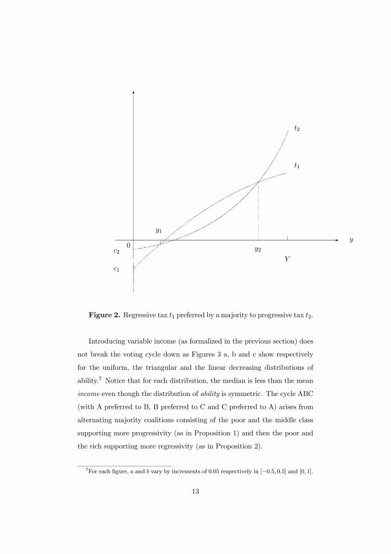
Proposition 2: (Hindriks, 2000) Suppose income is Þxed and distributed

according to F (y) in [0, Y ], with ym < y and Y large enough. Then for any

tax scheme t2 = −c2 + b2y + a2y2 there exists a less progressive tax schemet1 = −c1+b1y+a1y2 with a1 < a2 , b1 > b2 and c1 > c2 such that a majorityof voters prefers t1 over t2.

Proof: see Hindriks (2000).

Figure 2 illustrates this proposition. t1 is preferred by a majority to t2 if

the probability mass on the interval [y1, y2] is less than 1/2. Notice that the

result is true irrespective of the form of the income distribution, provided

that the median is less than the mean income.6 This result is not trivial.

Indeed the average income y is always lying within [y1, y2] and the lower the

probability mass around y, the greater the length of [y1, y2].

6It can be shown that the result does not hold for symmetric distributions.

12

-

6

t2

t1

y2

Y

y

y1

c2

c1

0

Figure 2. Regressive tax t1 preferred by a majority to progressive tax t2.

Introducing variable income (as formalized in the previous section) does

not break the voting cycle down as Figures 3 a, b and c show respectively

for the uniform, the triangular and the linear decreasing distributions of

ability.7 Notice that for each distribution, the median is less than the mean

income even though the distribution of ability is symmetric. The cycle ABC

(with A preferred to B, B preferred to C and C preferred to A) arises from

alternating majority coalitions consisting of the poor and the middle class

supporting more progressivity (as in Proposition 1) and then the poor and

the rich supporting more regressivity (as in Proposition 2).

7For each Þgure, a and b vary by increments of 0.05 respectively in [−0.5, 0.5] and [0, 1].

13

Insert Figures 3 a, b, c

In the following sections we shall see how we can escape this vote cycling

difficulty and gain insight on which tax functions have a chance to emerge

as political equilibria: Þrst by reducing naturally the voting space (Section

4), then by applying weaker political equilibrium concepts (Section 5); and

lastly by assuming that political parties also care about the size of their

majority (Section 6).

4 Natural reduction of the policy space

In this section, we restrict the policy space to the set of feasible tax schedules

that are most-preferred by some voter. This assumption seems a natural way

to reduce the policy space, and has been successfully adopted by Snyder and

Kramer (1988) enabling them to obtain a Condorcet winner with progressive

taxation.8 This reduction of the policy space can also be motivated in

the line of the Citizen Candidates models as a lack of commitment from

candidates selected from the set of voters and who can only credibly propose

their most-preferred policy (see Osborne-Slivinsky, 1996, and Besley-Coate,

1997).

In Figures 4 a,b,c we have represented the bliss points of the electorate

for the three distributions of ability we are considering.9 Surprisingly the

distribution of bliss points has a similar form for each ability distribution.

The lowest-ability individual prefers the policy that maximizes c (i.e., the

peak of the Laffer surface). This is the regressive tax schedule, with the

highest b and the lowest a < 0, namely the top of the upper curve in the

distribution of bliss points. The second lowest-ability individual prefers a

8However, their model differs from ours in the sense that individuals do not respondto taxation by substituting untaxable leisure to taxable labor, but rather by working inan untaxed sector with lower wage rate.

9For each Þgure, a and b vary by increment of 0.005 respectively in [−0.5, 0.5] and [0, 1],that is they take on 200 different values each.

14

slightly less regressive tax (lower b for a slightly higher a), and so on moving

downwards along the upper curve as ability increases, until we reach a voter

with an ability close to the median who prefers the progressive tax policy

with b = 0 and the highest a > 0. From that point on we move to the

left along the horizontal axis as ability increases, involving less and less

progressivity as a decreases. Then we reach the median ability individual

who prefers (am, bm) = (0.285, 0), (0.25, 0) and (−0.15, 0.4) for the uniform,the triangular and the linear decreasing distributions, respectively. The

move to the left (lower a) continues as ability further increases, moving

progressively upwards along the lower curve. This lower curve is in fact the

lower bound of the feasibility condition (19) which means that all these bliss

points are in fact constrained by the feasibility condition b > b(a).

Figures 4 a,b,c

We can now put the bliss points by increasing order of ability and derive

the (indirect) utility function of each voter over this distribution of bliss

points. Interestingly enough we obtain that for the three distributions of

ability, each voter displays single-peaked preference over this ordered set of

bliss points. Therefore it follows from the median voter theorem that the

bliss point of the median voter is a Condorcet winner.10 Since the median

voter is also the more favourable to progressivity we get a Þrst possible

explanation for the prevalence of progressive taxation.11

In the following section, instead of reducing the policy space we study

weaker solution concepts in the context of a standard Downsian political

competition game.

10Roell (1997) obtains a similar result with quasi-linear preferences. We thank RobinBoadway for pointing out this paper to our attention.11In the case of the linearly decreasing distribution of ability, the median ability is so

low that the median voter prefers regressivity like the low-ability voters.

15

5 The simultaneous two-party competition game

We consider a Downsian voting game with two political parties competing to

win the election. Both parties simultaneously announce their tax schedule

(a pair (a, b)) which they commit to impose if elected. Each individual then

votes for the party whose platform is better according to his/her preferences.

The party receiving the most votes wins the election and imposes its platform

as the choice of the polity. In the event of ties, a fair coin decides which

party wins the election. Note that in constrast with Section 4, it is assumed

here that candidates can commit to any policy.

Formally, we denote the (Þnite) set of feasible policies by X. An element

of X is thus a pair (a, b). Let P denote the majority preference relation on

this set X. The majority preference P over any policy pair (x, y) ∈ X2 is

given by,

xPy : n(x, y) > n(y, x)yPx : n(x, y) < n(y, x),

where n(x, y) = #{w ∈ [0, 1] : v(x;w) > v(y;w)} is the number of voterswho (weakly) prefer x to y, and n(y, x) = #{w ∈ [0, 1] : v(x;w) < v(y;w)}is the number of voters who prefer y to x.12

Assuming an odd number of voters, the majority preference relation is a

binary relation satisfying the asymmetry and completeness properties of a

tournament.

The objectives assigned to the parties are crucial. We suppose that par-

ties are only interested in winning the election and that they derive no in-

trinsic utility from the platform chosen (i.e., no ideology). Moreover parties

are indifferent about the size of their majority: having a bare majority they

attach no utility to any extra vote. Given that parties can choose among

12We rule out indifference since it is a very unlikely event.

16

the same set of feasible policies, we can represent this electoral competition

by a symmetric two-player zero-sum game G = (X,X,U) where:

U(x, y) =

1 : xPy

−1 : yPx0 : x = y

This game, called the majority game, has a unique Nash equilibrium in

pure strategies if and only if there exists a Condorcet winner. Formally,

x ∈ X is a Condorcet winner if and only if xPy for all y ∈ X\{x}. In thiscase, both parties choose the Condorcet winner as a strategy.

But we know from Section 3 that there is no Condorcet winner in the

(unrestricted) two-dimensional policy space. It follows that the game does

not have any equilibrium in pure strategies: each party could win the election

if it knew which policy is chosen by the other party.13

However, the absence of a Condorcet winner does not imply that any policy

is equally likely to be selected by any party. First, we do not expect any

party to select a Pareto dominated policy x (like a > 0 and b > 1/3).

Second, we feel conÞdent that any party is unlikely to propose weakly

dominated policies. A policy x is weakly dominated by policy y if U (x, z) ≥U (y, z) for all z ∈ X, with a strict inequality for at least one z. Reformulatedin our voting context, y weakly dominating x means that y beats x as well

as any policy z that x can beat.

In the social choice literature, this dominance relation is also called the

covering relation (see Miller, 1980). Formally, given a tournament (X,P ),

a policy x ∈ X is covered whenever there exists some other policy y ∈ Xsuch that yPx and {z : xPz} ⊆ {z : yPz}. The set of non-covered optionsfor the majority preference relation P is called the uncovered set, denoted

UC(X,P ). Since the covering relation is equivalent to the weak dominance

13This is in contrast to Cukierman and Meltzer (1991) who make very restrictive as-sumptions on the ability distribution and voters� preferences to get the existence of aCondorcet winner over quadratic income tax schemes. In our model even with very sim-ple preferences and ability distributions the Condorcet winner fails to exist.

17

relation in our setting, the uncovered set is precisely the set of weakly un-

dominated pure strategies of the two-party zero-sum game G = {X,X,U}.Given that any Pareto-dominated policy is covered, the uncovered set is a

subset of the Pareto set.14

We can further restrict the set of interesting strategies by looking at the

Nash equilibrium in pure strategies of this game.15 Laffond et al. (1993)

have shown that the Þnite and symmetric majority game G = (X,X,U)

has a unique equilibrium in mixed strategies. They call the support of this

unique equilibrium the bipartisan set denoted BP (X,P ).16 It can be shown

that the bipartisan set is a subset of the uncovered set and thus a more

discriminating solution concept (see Banks et al., 1996). Furthermore, both

the uncovered set and the bipartisan set reduce to the Condorcet winner

when the latter exists.

Given these deÞnitions, we can now compute the Pareto set, the uncov-

ered set and the bipartisan set for the three distributions of ability. The

results are reported below.17

Insert Figures 5 a,b,c

As Figures 5 a,b,c indicate the distribution of abilities matters a lot in

determining whether progressive taxation is likely to emerge in equilibrium.

With a triangular distribution (Figure 5b), regressive taxes are weakly dom-

inated (and a fortiori are never played in the mixed strategies Nash equi-

librium). The reason is that this symmetric distribution implies a large

14If x is Pareto-dominated by y, y has a better position than x in every individualpreference ordering. Hence, using majority voting, y beats all the options that x beats,which means that y covers x.15See Laslier(2000) for an interpretation of electoral mixed strategies16The bipartisan set is thus the set of options played with a strictly positive probability

at the equilibrium.17For each Þgure, a and b vary by increment of 0.05 respectively in [−0.5, 0.5] and [0, 1].

18

middle income group who can impose progressivity in order to reduce its

own tax burden at the expense of the high-income group. The reverse holds

when we shift the probability mass to the low ability levels as with the lin-

ear decreasing distribution (Figure 5c). In this case, the low-income group

becomes sufficiently large to impose regressive taxes in order to maximize

tax revenue (and thus redistribution). When ability levels are uniformly

distributed (Figure 5a), then both regressive and progressive taxation can

emerge in equilibrium. Therefore, these results suggest that the prevalence

of progressive taxation can only be explained by the predominance of the

middle class in the income distribution or equivalently by a lack of polariza-

tion at the extremes of the income distribution. Figures 5a,b,c also reveal

that the Uncovered set and the Bipartisan set are very discriminating so-

lution concepts. This is in contrast to Epstein (1997) who shows that for

games of purely distributive politics the Uncovered set coincides approx-

imately with the Pareto set. Our results demonstrate that for the game

studied here, the Uncovered set (and a fortiori the Bipartisan set) can give

rather sharp predictions on equilibrium outcomes.

In the next section we analyse how it is possible to get better predictions

on the equilibrium outcomes by changing the rules which dictate the play

of the game instead of changing the equilibrium concept.

6 The sequential two-party competition game

We use the dynamic version of the two-party electoral competition game

due to Kramer (1977). In this voting game, two political parties repeatedly

compete for the votes with the peculiarity that when a party is elected, it

is committed to keep the same political platform for the next election (rep-

utation inertia). In absence of Condorcet winner, this assumption implies

that both parties alternate in office because each party can win the election

once it knows the policy chosen by the other party. It is further assumed

19

that parties are interested in maximizing the size of their majority (or net

plurality deÞned as n(x, y)−n(y, x)), and thus the opposition party will al-ways select a policy which maximizes its voting share given the incumbent�s

policy. This dynamic voting process can be represented by the sequence of

winning policies, which Kramer calls a vote-maximizing trajectory (i.e., a

sequence of policies such that each policy along the sequence beats with a

maximal number of votes its predecessor). Formally, for any two adjacent

policies (xt, xt+1) along the sequence, xt+1 ∈ argmaxy∈X n(y, xt).

Using our model, we have simulated the Kramer trajectories for the

three distributions of ability. The results are reported in Figures 6a,b,c.18

For each distribution, we get that the Kramer trajectory converges to a cy-

cle which is independent of the initial point. For each distribution we move

clockwise along the cycle with a coalition of the extremes alternating with

a coalition of the middle and low-income groups.

Figures 6 a,b,c

We have also represented the minmax set which is deÞned as the set

of policies whose maximal opposition is minimal. Formally, minmax(X) =

argminxmaxy 6=xn(y, x). Kramer has demonstrated that for Euclidean pref-

erences the minmax set behaves like a basin of attraction in the sense that

any vote-maximizing trajectory converges to the minmax set. As shown

below, for the model used here (with non-Euclidian preferences), we obtain

that Kramer cycles always pass through the minmax set (which may reduce

to a singleton).

According to these simulation results, the prevalence of progressive taxa-

tion can only be explained, as for the Bipartisan and the Uncovered sets, by

the predominance of the middle class in the income distribution. Indeed only

18For each Þgure, a and b vary by increment of 0.025 respectively in [−0.5, 0.5] and [0, 1].

20

the triangular distribution (Figure 6b) with a lack of polarization at the ex-

tremes produces a Kramer cycle that only contains progressive taxes. Shift-

ing the probability mass of individual abilities evenly towards the extremes

(Figure 6a) makes the vote maximizing trajectory cycles evenly between re-

gressive and progressive taxes; while a high probability mass at low-ability

levels (Figure 6c) induces a Kramer cycle that only contains regressive taxes.

7 Conclusion

This paper is an attempt to explain the prevalence of income tax progressiv-

ity in a positive rather than normative perspective. We have used a highly

stylized model that nevertheless includes the salient aspects of voting over

non-linear income tax schedules. We have Þrst shown that voting cycles over

the set of progressive and regressive taxes is inevitable when taxation is not

distortionary: progressive taxes (or convex tax function) enables the mid-

dle class to reduce its tax burden at the expense of the high-income group;

while regressive taxes (concave tax function) reduces the tax burden at the

extremes at the expense of the middle-class.

Introducing incentive effects allows us to take account of the fact that

progressivity discourages effort which to some extent ticks the model in fa-

vor of regressive taxes. However we show that vote cycling over progressive

and regressive taxes still prevails in the presence of incentive effects. Then

we consider three different ways to give better predictions on the voting out-

come and more importantly to explain the prevalence of progressive taxes.

The Þrst approach reduces the policy space to the tax schedules that are

ideal for some voter. In that case we obtain a Condorcet winner corre-

sponding to the policy preferred by the median voter. The second approach

considers the entire policy space, but adopts weaker solution concepts in the

context of a simultaneous two-party competition game. The third approach

21

considers a sequential two-party competition game in which parties not only

care about winning, but also about the size of their majority.

The main result is that whatever the approach adopted, progressive taxes

emerge as the only possible voting outcome when there is a lack of polar-

ization at the extremes of the income distribution. In this exercise, we do

not pretend we have succeeded in capturing the reason of the revealed pref-

erence for progressive income taxation, but perhaps we have captured some

of its ground. Further research is of course needed to solve this demand for

progressivity puzzle.

Acknowledgements. This paper was prepared for presentation at the

ISPE conference on Public Finance and Redistribution at CORE, Belgium,

June 2000. We wish to thank our discussants Gerard Roland and David

Wildasin for helpful comments. We also thank participants at the Public

Economics conference of the AFSE in Marseille, May 2000. This paper was

initiated while Jean Hindriks was visiting the Institut d�Economie Indus-

trielle (IDEI-CERAS-GREMAQ) in Toulouse, whose Þnancial support and

hospitality are gratefully acknowledged. The usual disclaimer applies.

22

References

[1] Banks, J., J. Duggan and M. Le Breton, 1998, Bounds for mixed strate-

gies equilibria and the spatial theory of elections, mimeo, University of

Rochester.

[2] Besley, T. and S. Coate, 1997, An Economic Model of Representative

Democracy, Quarterly Journal of Economics , 112, 85-114

[3] Cukierman A., A. Meltzer, 1991, A political theory of progressive in-

come taxation, in Political Economy , by A. Meltzer, A. Cukierman

and S.F. Richard.(Eds.). Oxford University Press. New York.

[4] De Donder, P., J. Hindriks (1998). The political economy of targeting,

Public Choice, 95, 177-200.

[5] De Donder, P., M. Le Breton and M. Truchon, 2000, Choosing from a

weighted tournament, Mathematical Social Science, forthcoming.

[6] Epstein, D., 1997, Uncovering some subtleties of the uncovered set:

social choice theory and distributive politics, Social Choice and Welfare,

15, 81-93.

[7] Hindriks, J., 2000, Is there a demand for progressive taxation?, mimeo

QMW.

[8] Kramer, G., 1972, Sophisticated voting over multidimensional choice

spaces, Journal of Mathematical Sociology, 2, 165-80.

[9] Kramer, G., 1977, A dynamic model of political equilibrium, Journal

of Economic Theory, 16, 310-34.

[10] Kramer, G., 1983, Is there a demand for progressivity?, Public Choice,

41, 223-28.

[11] Laffond, G., J.F. Laslier and M. Le Breton, 1993, The bipartisan set of

a tournament game, Games and Economic Behavior, 5, 182-201.

23

[12] Laslier, J.F., 2000, Interpretation of Electoral Mixed Strategies, Social

Choice and Welfare, 17-2, 283-292.

[13] Laslier, J.-F., A. Trannoy, K. Van der straten, 2000, Voting under igno-

rance of unemployed job skills: the overtaxation bias, mimeo THEMA.

[14] Marhuenda, F., I. Ortuno-Ortin, 1995, Popular support for progressive

taxation, Economics Letters,48, 319-24.

[15] Miller, N., 1980, A new solution set for tournaments and majority vot-

ing, American Journal of Political Science, 24, 68-96.

[16] Mitra, T., E. Ok, L. Kockesen, 1998, Popular support for progressive

taxation and the relative income hypothesis, Economics Letters, 58,

69-76.

[17] Myles, G., 2000, On the optimal marginal rate of income taxation,

Economics Letters, 113-19.

[18] Osborne, M.J., A. Slivinski, 1996, A Model of Political Competition

with Citizen candidates, Quarterly Journal of Economics, 111, 65-96.

[19] Plott, C.R., 1967, A Notion of Equilibrium and its Possibility under

Majority Rule, American Economic Review, 57, 787-806

[20] Roberts, K., 1977, Voting over income tax schedules, Journal of Public

Economics, 8, 329-40.

[21] Roell, A., 1997, Voting over non-linear income tax schedules, mimeo

Tilburg University.

[22] Roemer, J., 1999, The democratic political economy of progressive in-

come taxation, Econometrica, 67, 1-19.

[23] Romer, T., 1975, Individual Welfare, Majority Voting, and the Proper-

ties of a Linear Income Tax, Journal of Public Economics , 4, 163-185.

24

[24] Snyder, J. and G. Kramer, 1988, Fairness, self-interest, and the politics

of the progressive income tax, Journal of Public economics, 36, 197-230.

[25] Stigler, G.J., 1970, Directors� law of income distribution, Journal of

Law and Economics, 13, 1-10.

[26] Young, P., 1990, Progressive taxation and equal sacriÞce, American

Economic Review, 80, 253-66.

25

Figure 3a: Majority voting cycle with uniform distribution

C

B

A

0

0.1

0.2

0.3

0.4

0.5

0.6

0.7

-0.4 -0.3 -0.2 -0.1 0 0.1 0.2 0.3

a

b

Figure 3b: Majority voting cycle with triangular distribution

C

B

A

0

0.1

0.2

0.3

0.4

0.5

0.6

-0.35 -0.3 -0.25 -0.2 -0.15 -0.1 -0.05 0 0.05 0.1 0.15 0.2

a

b

Figure 3c: Majority voting cycle with linearly decreasing distribution

C

B

A

0

0.1

0.2

0.3

0.4

0.5

0.6

-0.4 -0.3 -0.2 -0.1 0 0.1 0.2 0.3

a

b

Figure 4a: Voters' blisspoints with uniform distribution of abilities

0.00

0.10

0.20

0.30

0.40

0.50

0.60

0.70

0.80

-0.50 -0.40 -0.30 -0.20 -0.10 0.00 0.10 0.20 0.30 0.40 0.50

a

b blisspointsmedian individual's blisspoint

Figure 4b: Voters' blisspoints with triangular distribution of abilities

0.00

0.10

0.20

0.30

0.40

0.50

0.60

0.70

-0.60 -0.50 -0.40 -0.30 -0.20 -0.10 0.00 0.10 0.20 0.30 0.40 0.50

a

b blisspointsmedian individual's blisspoint

Figure 4c: Voters' blisspoints with linearly decreasing distribution of abilities

0.00

0.10

0.20

0.30

0.40

0.50

0.60

0.70

-0.60 -0.40 -0.20 0.00 0.20 0.40 0.60

a

b blisspointsmedian individual's blisspoint

Figure 5a: Pareto set, Uncover set and Bipartisan set for the uniform distribution of abilities

0

0.1

0.2

0.3

0.4

0.5

0.6

0.7

0.8

0.9

1

-0.5 -0.4 -0.3 -0.2 -0.1 0 0.1 0.2 0.3 0.4 0.5

a

b

Uncovered setBipartisanPareto frontier

Figure 5b: Pareto set, Uncover set and Bipartisan set for the triangular distribution of abilities

0

0.1

0.2

0.3

0.4

0.5

0.6

0.7

0.8

0.9

1

-0.5 -0.4 -0.3 -0.2 -0.1 0 0.1 0.2 0.3 0.4 0.5

a

b

Uncovered setBipartisanPareto frontier

Figure 5c: Pareto set, Uncover set and Bipartisan set for the linearly decreasing distribution of abilities

0

0.1

0.2

0.3

0.4

0.5

0.6

0.7

0.8

0.9

1

-0.5 -0.4 -0.3 -0.2 -0.1 0 0.1 0.2 0.3 0.4 0.5

a

b

Uncovered setBipartisanPareto frontier

Figure 6a: Kramer cycle and minmax with uniform distribution of abilities

0

0.05

0.1

0.15

0.2

0.25

0.3

0.35

0.4

0.45

-0.2 -0.15 -0.1 -0.05 0 0.05 0.1 0.15 0.2 0.25 0.3

a

b Kramer cycleminmax

Figure 6b: Kramer cycle and minmax with triangular distribution of abilities

0

0.05

0.1

0.15

0.2

0.25

0.3

-0.2 -0.15 -0.1 -0.05 0 0.05 0.1 0.15 0.2 0.25

a

b kramer cycleminmax

Figure 6c: Kramer cycle and minmax with linearly drecreasing distribution of abilities

0

0.05

0.1

0.15

0.2

0.25

0.3

0.35

0.4

0.45

0.5

-0.3 -0.25 -0.2 -0.15 -0.1 -0.05 0 0.05 0.1 0.15 0.2

a

b Kramer cycleminmax point