the phillips curve in australia - old dominion...
TRANSCRIPT

THE PHILLIPS CURVE IN AUSTRALIA
David Gruen*, Adrian Pagan** and Christopher Thompson*
Research Discussion Paper1999-01
January 1999
*Economic Research Department, Reserve Bank of Australia**Australian National University
Adrian Pagan is a member of the Board of the Reserve Bank of Australia. Anearlier version of this paper was presented at the StudienzentrumGerzensee/Journal of Monetary Economics conference on ‘The Return of thePhillips Curve’, 7–10 October 1998. We would like to thank Larry Christiano,Graham Elliot, Neil Ericsson, Graeme Wells and other conference participants fortheir comments on the earlier version of this paper. The views expressed in thispaper are those of the authors and should not be attributed to the Reserve Bank ofAustralia.

i
Abstract
In this paper we discuss the development of Phillips curves in Australia over theforty years since Phillips first estimated one using Australian data. We examine thecentral issues faced by researchers estimating Australian Phillips curves. Theseinclude the distinction between the short and long-run trade-offs between inflationand unemployment, and the changing level of the non-accelerating inflation rate ofunemployment (NAIRU), particularly in the 1970s. We estimate Phillips curves forprices and unit labour costs in Australia over the past three decades. These Phillipscurves allow the NAIRU to change through time, and include a role for importprices and ‘speed-limit’ effects. The paper concludes by presenting an extendeddiscussion of the changing role of the Phillips curve in the intellectual frameworkused to analyse inflation within the Reserve Bank of Australia over the past threedecades.
JEL Classification Numbers: E24, E31, E52Keywords: Phillips curve, inflation, unemployment, monetary policy

ii
Table of Contents
1. Introduction 1
2. Early Studies of the Australian Phillips Curve 3
3. Recent Work on the Phillips Curve 16
4. The Phillips Curve and Monetary Policy 30
5. Conclusion 38
Appendix A: National Wage Case Outcomes (1968–1981) 41
Appendix B: Exogeneity Assumptions Relevant to Estimating Phillips Curves 42
Appendix C: Time-series Properties of the Variables 43
Appendix D: Technical Issues Involved in Estimating the Kalman Filter 44
Appendix E: Data Description and Sources 49
References 52

THE PHILLIPS CURVE IN AUSTRALIA
David Gruen, Adrian Pagan and Christopher Thompson
1. Introduction
In 1959, A.W. (Bill) Phillips spent a sabbatical year in Australia at the Universityof Melbourne. During his time there he produced what might have been the second‘Phillips curve’ in the world. Since that time Phillips curves have appeared formany countries under many guises, have found their way into textbooks andconferences, and have become part of the standard set of tools available tomacroeconomists when thinking about the effects of policy actions. At the sametime, it has become apparent that there is no real agreement over exactly what theterm ‘Phillips curve’ implies. The original concept of the equation related wageinflation to unemployment, but modern versions are as likely to relate priceinflation to ‘output gaps’. The diverse uses to which Phillips curves have been putcan be seen from the trinity of benefits that Stiglitz (1997) mentions as accruingfrom the possession of a Phillips curve:
1. It is useful for describing the determinants of inflation.
2. It is useful in providing a framework for policy.
3. It is useful for forecasting inflation.
As might be expected, it is unlikely that a single curve can be used for all threepurposes. When forecasting or explaining history the curve might have to beaugmented with a large array of variables representing both demand and supplyinfluences and institutional factors relating to price and wage controls. Goodexamples of such a curve are the ‘triangle’ models of Gordon (1997). However,when it comes to establishing a policy framework, simpler versions of the curvemay be desirable. Moreover, since policy has to be set within a systems context, asingle equation can only be regarded as one of the building blocks of a system.Tensions created by the need to address such a range of issues have been evidentboth in the Australian and wider literatures and partly account for the large numberof Phillips curves that have been estimated. Because of this, it is useful to havesome way of organising the discussion, and the trinity of uses distinguished above
2
is a convenient way of summarising its main conclusions. It is what we do in thepresent paper, although we focus only upon the first two items in the list.
The next section of this paper sets out a general framework that has been the basisof much work on the Phillips curve in Australia. It involves fairly standarddescriptions of mark-up pricing and expectations-augmented wage curves, withadjustments made to reflect the fact that Australia is a small, open economy. Theframework has been used within the Reserve Bank to study issues such as inflationtargeting (for example, see de Brouwer and O’Regan (1997)). Furthermore, sincemany of the important studies of the Phillips curve in Australia emerged from theResearch Department of the Reserve Bank, and since the people involved in thesestudies also had some input into the formulation of monetary policy, it is of interestto pay special attention to them.
Section 2 derives Phillips curves that reflect most of the historical research on thesubject in Australia. Because this work has exhibited a dual focus, sometimestreating the Phillips curve as determining price inflation and sometimes labour costmovements, we derive two such curves. This duality is a feature of the paper,although, as will become clear, our preference is for the labour cost version. Inconducting the research we also make some general comments about thedifficulties faced by those endeavouring to estimate a Phillips curve for Australia.
Most of the research discussed in Section 2 is aimed at satisfying the first item inStiglitz’ list in that it seeks to provide a list of variables that are likely to be mostinfluential in producing a change in inflation. While an understanding of suchdeterminants is important, for policy there can be little doubt that it is the NAIRUand its measurement that comes to the fore, and the Phillips curve has frequentlybeen used in this endeavour. Of course, there are well known difficulties in using aPhillips curve for this purpose and these are accentuated in the Australian casebecause the NAIRU has clearly not been constant over the past three decades.Consequently, in Section 3, we examine the significant recent contribution ofDebelle and Vickery (1997) in which the NAIRU is allowed to change throughtime. Because Debelle and Vickery’s model is a simpler specification than mostPhillips curves recently estimated, we derive a richer specification which includesadditional relevant regressors. Our results imply estimates of the NAIRU in 1997of around 5½–7 per cent. We also examine whether the NAIRU depends, in a

3
systematic way, on changes in the replacement ratio or in the proportion oflong-term unemployed, although we are unable to find such dependence.
In Section 4 of the paper we look at the role of the Phillips curve in providing aframework for the formulation of monetary policy in Australia. We discuss thechanging views about the Phillips curve within the Reserve Bank over the pastthree decades, and examine how these views have informed analysis of theinflationary process in Australia. Although the importance of the Phillips curveframework has fluctuated over the years, it currently has an influence comparableto that in the early 1970s when the (expectations-augmented) Phillips curve wasfirst embraced to explain stagflation. The paper ends with a brief conclusion.
2. Early Studies of the Australian Phillips Curve
Phillips curve research within Australia can be usefully encapsulated within thecontext of the following three equations:
tjtktktk xPMULCcP 1321 lnlnln ��� ������� � (1)
tte
tktk xzPULC 2lnln ��� ����� (2)
� � ttke
tk xPP 31ln1ln �� �����-
. (3)
In Equation (1), tP is the consumer price level excluding interest rates and othervolatile items, and its rate of change is the underlying inflation rate, until recentlythe series targeted by the Reserve Bank of Australia.1 tULC is unit labour costsand tPM is tariff-adjusted import prices. The presence of import prices reflects thefact that a significant proportion of goods consumed within Australia are imported
1 As discussed later, the Reserve Bank has a target for inflation of 2�3 per cent per annum onaverage over the medium term. This target was expressed in terms of underlying inflationuntil October 1998.

4
and that the cost structure of Australian industry is affected by imported goods aswell.2 The second of the equations describes the evolution of unit labour costs. Inmost studies of the Phillips curve that have concentrated on labour compensation,
tULC is decomposed into its components of wages and productivity growth. Wagemovements, or more broadly unit labour costs, are driven by expectations of theprice level e
tP , by ‘demand factors’ tz , and ‘other’ factors tx2 . Finally,expectations are modelled by combining a backward-looking component and someother (possibly forward-looking) measure, tx3 . The unit of observation is usually aquarter (since both price and wage data are available with that frequency) and thechoice of k in �k determines the period over which wage and price movements aremeasured. Setting 4�k produces annual wage and price movements.
Phillips’ (1959) Australian version of his classic paper estimated a wage version ofEquation (2) with quarterly data and 4�k .3 However, compared with his Britishwork there were some significant changes, mostly in response to the institutionsgoverning the way in which Australian wages were set. Until the 1990s, wagesetting in Australia was quite centralised and distinctive. A legal system set awardand minimum wages for most industries and ‘collective bargaining’ amounted tounions and employers arguing cases before an Arbitration Court, which madedecisions regarding award wage changes. Thus, the equations Phillips presentedwere based on wage inflation that was closer to ‘award wages’ than actual‘earnings’; the difference, frequently referred to as ‘earnings drift’, arose fromstrong unions’ capacity to negotiate above-award wages outside the ArbitrationCourt system. His equations also featured unemployment as well as import andexport price inflation. The influence of the institutional features upon his thinking
2 Gali and Gertler (1998) effectively consider a model in which tP is a mark-up over tULC . In
our data set tPln and tULCln are I(1) processes and a dynamic equilibrium mark-up model
would naturally be formulated in an error correction form. In this case, Equation (1) wouldinclude an error correction term which could be interpreted as the labour share of income.de Brouwer and Ericsson (1995, 1998) include such a term in their model of Australianinflation, but over our sample period this term does not appear to be stationary. Moreover,when it is added to the Phillips curve equations which we estimate in Section 3, it is ofmarginal significance.
3 Perry (1980) and Pitchford (1998) provide good discussions of this paper.

5
was particularly evident in the comments he made about the effects of the latterupon wages:
It seems that the decisions of the Arbitration Court were strongly affected by therapidly rising export prices…
(Phillips 1959, p. 3)
The importance of the courts in determining wage inflation in Australia wasmanifested in many ways. As well as cases relating to specific industries, one had‘National Wage Cases’ in which the whole structure of awards was generallyadjusted upwards. The table in Appendix A details the outcomes of each of theseNational Wage cases between 1968 and 1981 (the end of wage indexation inAustralia) and also gives the change in average earnings in the year after eachdecision came into effect. The exact timing and magnitude of these decisionsrendered quarterly movements in wages very erratic, which even conversion toannual changes could not entirely smooth out (Figure 1). Such a series, particularlythe quarterly one, may be hard to model.
Figure 1: Unit Labour Cost InflationPercentage change
-10
-5
0
5
10
15
20
25
30
35
-10
-5
0
5
10
15
20
25
30
35
1997
%
Annual
Quarterly (Annualised)%
19931989198519811977197319691965

6
Two responses could be made to the erratic movements evident inFigure 1. First, one might treat the Phillips curve as determining prices rather thanwages. Pitchford (1968) seems to have been the first to do this in Australia,although it had been popular in the US for some time. A useful benchmark Phillipscurve involving price inflation, that we will frequently refer back to later, isconstructed from the following two equations:
te
tt zPP �� ���� lnln 44 (4)
� � *144 ln1ln tt
et PPP ������
-
�� , (5)
where *tP� is a measure of expected inflation and tz measures ‘excess demand’.
Almost all of the early work on the Phillips curve in Australia (including Phillips(1959)) accepted that there was a trade-off between inflation and unemployment,even in the ‘long-run’. In the early 1970s, however, this proposition wasincreasingly questioned and a lot of time was spent testing whether a long-runtrade-off actually existed, i.e. whether 1�� . As we discuss later, Michael Parkinwas an influential figure in that debate and Chart 1 in Parkin (1973, p. 135)suggests that the estimates made of � had been slowly converging on unity.4
Henceforth, we assume that 1�� . Doing so, and replacing tz with the difference
4 The proposition that 1�� could be tested because the relevant studies modelled wages rather
than prices. Given any information set used by agents, one could replace etk Pln� with
tk Pln� and then instrument tk Pln� with elements of that set, provided the instruments were
not correlated with the error term of the wage equation. To ensure this, the minimalinformation set was assumed to be composed of award wages, overseas prices andproductivity movements (in fact, instrumental variables estimation was rarely performeddirectly but rather these three instruments were substituted for the actual inflation rate and arestriction was imposed upon the three weights, that they added to unity, thereby reducing thethree unknown weights to two). It was therefore possible to avoid the Lucas/Sargent critiqueby working with a wage equation (a strategy that would clearly fail if one had price ratherthan wage inflation as the dependent variable). We do not comment further on this debatehere.

7
between the unemployment rate tU and the NAIRU *tU , enables us to
reparameterize Equations (4) and (5) as:
� � � �*14
*144 lnlnln tttttt UUPPPP ���������
--
�� . (6)
Furthermore, if the NAIRU is constant, Equation (6) may be re-written as:
� � ttttt UPPaPP �� ���������-- 14
*144 lnlnln , (7)
where *Ua ��� .
Equation (6) is a useful specification which we will retain in later work. By makingthe acceleration in inflation the dependent variable, the equation becomes one thatinvolves an ‘accelerationist’ form of the Phillips curve. If the NAIRU is constant,
*U can be treated as a parameter and then Equation (6) can be estimated as anon-linear regression (alternatively, Equation (7) could be estimated as an OLSregression and *U recovered from the estimated parameters a and � ).
To estimate Equation (6), we first replace tU with � �tU4MA , where 4MA is afourth-order moving-average operator.5 Second, we use inflation expectationscomputed by Debelle and Vickery (1997) from bond yield data to represent *
tP� .6
In this, and all subsequent estimations, log levels and their differences aremultiplied by 100. Estimating Equation (6) as a non-linear regression over theperiod 1965:Q2–1997:Q4 gives (with absolute values of t-ratios in brackets):
)88.6(%41.5)46.3(095.0)62.2(070.0 * ���� U�� .
5 If one does not do this then a transitory rise in the unemployment rate will have a peculiareffect upon quarterly inflation rates due to the fact that the annual inflation rate is just the sumof the quarterly inflation rates. Specifically, these would fall in the first quarter then rise insubsequent quarters. In practice, it makes almost no difference to the point estimates whetherwe use tU or � �tU4MA as the tU series is already very smooth. Many studies have used
� �tU4MA , e.g. Jonson, Mahar and Thompson (1973).6 Appendix E contains descriptions and the sources for the data which we use in this paper.

8
While the signs are as expected, the fit is very bad, with 09.02 �R and91.0�DW . Moreover, fitting the relation over the sub-period 1965:Q2–1976:Q1
generates an estimate of %2.2* �U , indicating that the relation has not beenparticularly stable.
Table 1 summarises early research on wage and price Phillips curves in Australia.When it came to modelling wage inflation, rather than price inflation, researchersin policy institutions mostly examined movements in labour costs conditional uponthe decisions taken by the Arbitration Court. Technically, tx2 in Equation (2) wasset to changes in award wages and what was modelled was essentially ‘earningsdrift’, that is, the gap between award wages and those actually paid; somethinglikely to be affected by the state of the labour market. Some of these studies arealso summarised in Table 1. Of course, such a ‘solution’ was less helpful in aforecasting environment as some prediction needed to be made about futureArbitration Court decisions, i.e., an equation for tx2 was necessary. There were anumber of attempts to do this and Higgins (1973) and Jonson, Mahar andThompson (1973) were among the earliest of these studies. Generally, modellingof earnings given award wages was quite successful. In contrast, it was difficult tomodel either earnings without conditioning upon award wages or award wagesthemselves. Given the frequency of Arbitration Court decisions, it was probablyinevitable that annual wage movements ( 4�k ) became the preferred series tomodel.

9
Table 1: Summary of Early Phillips Curve Studies in AustraliaWage equations
Author(s) Dependent variableExcess labour
demandvariable(s)
Other variable(s)
Phillips (1959) Annual % change in wages 2/1 U � Import prices
� Export prices
Hancock (1966) Annual % change in wages UU ln,ln � � Minimum wages
Schott (1969) (a) Level of wages Level VU , � Company profits� Ratio of union
membership to labourforce
� Lagged price inflation
Jonson (1972) (a) Annual % change in wages U/1 � Inflation expectations(survey measure)
� Minimum wages� Working days lost due
to strikes
Parkin (1973) (a) Annual % change in wages � �UV
UU
�� ,/1,/1 � Award wages
� Productivity� Tradeables inflation
Higgins (1973) Annual % change in wages � �UVUV �, � Lagged price inflation� Award wages
Jonson, Mahar andThompson (1974) (a)
Annual % change in wages � �UVUV �, � Foreign reserves� Award wages� World prices� Productivity
Carmichael andBroadbent (1980) (a)
Quarterly % change in wages UV � � Inflation expectations
Kirby (1981) Quarterly % change in wages U � Inflation expectations(various measures)
Gregory (1986) Quarterly % change in wages OVU ,, � Dummy for 1974:Q3� Inflation expectations
(various measures)
Simes and Richardson(1987)
Quarterly % change in wages OU , � Lagged price inflation
continued next page

10
Table 1: Summary of Early Phillips Curve Studies in Australia (continued)
Price equations
Author(s) Dependent variableExcess labour
demandvariable(s)
Other variable(s)
Pitchford (1968) Annual % change in prices UV � � Export prices
� Import prices
� Minimum wages
� Productivity
Nevile (1977) Annual % change in prices UVU �, � World prices
� Indirect taxes
� Award wages
Notes: U is the unemployment rate (or level, where indicated).
V is the vacancy rate.
O is overtime hours worked.(a) These studies were undertaken in the Research Department of the Reserve Bank of Australia.
Equation (8) is an equation for unit labour costs that parallels the ‘price equation’in Equation (6):
� � � �*414
*144 )(MAlnlnln tttttt UUPPPULC ���������
--
�� . (8)
Estimates of its parameters over the period 1965:Q2–1997:Q4 are:
)07.14(%32.6)16.6(608.0)28.2(219.0 * ���� U��
with 23.02 �R and 49.0�DW .7 By and large, the effects are better determinedthan in the price equation. However, the instability in the price equation is also
7 Because the Phillips curve is a single equation in a system, our estimates of Equations (6)and (8) are based on some exogeneity assumptions. Appendix B contains a discussion of theexogeneity assumptions relevant to estimating Phillips curves.

11
present in the wage equation, with an estimated NAIRU over the earliersub-sample (1965:Q2–1976:Q1) of 2.5 per cent.8
How might one improve upon the specifications of these two Phillips curveequations? As mentioned earlier, it is unlikely that one could capture the impact ofimport prices upon final goods prices with what is effectively just wage pressures.Moreover, there may be ‘speed-limit’ effects, so that a rapid change in theunemployment rate has an impact on prices, implying that the demand measuremight also include changes in the unemployment rate. Finally, there is a decision tobe made about whether to model quarterly or annual movements in wages andprices. We choose to model annual movements, which leads us to the followingspecification for the change in annual price inflation:9
� � � �� � � � .lnlnlnln
MAlnlnln
41224141
1414*
144
----
---
�������������������
tttt
tttttt
PPPMPM
UdUPPaPP
����
(9)
8 One response to this instability by earlier researchers was to experiment with differentmeasures of demand pressure. Stimulated by the emerging literature on the role of ‘insiders’and ‘outsiders’ in the wage-setting process, a range of these demand pressure variables havebeen proposed. For example, Gregory (1986) looked at overtime hours worked whileCockerell and Russell (1995) constructed a measure of ‘inside unemployment’. Neither ofthese alternatives produces much of an improvement in our equations though; with overtimethe crucial fit statistics are 19.02 �R and 53.0�DW , while using inside unemploymentresults in 23.02 �R and 60.0�DW .
9 As observed previously, annual movements were favoured in early work on the Phillips curvebut, after Kirby (1981), there was a shift towards modelling quarterly wage and pricemovements. From an economic viewpoint, it is of more interest to explain annual movementsin inflation than quarterly movements. This explains our choice of dependent variable inEquation (9). Consider deriving Equation (9) from an equation that has quarterly inflation( tPln� ) as the dependent variable and three lagged changes in quarterly inflation
( 31,ln ���-
jP jt ) as regressors. These regressors have associated coefficients j� . Since
annual inflation is the sum of four consecutive quarterly price changes, changing to annualinflation as the dependent variable simply means that the regressors jtP
-
� ln now have
coefficients ( j��1 ). In an equation with annual inflation as the dependent variable, the
coefficients on these regressors can be freely estimated, and any restrictions upon the j� can
be tested and imposed.

12
Since the dependent variable in this equation is the change in annual inflation, theaugmented list of regressors is extended to include 4ln
-
� tP . When the four laggedquarterly inflation rates are added to the regressor set we find that 1ln
-
� tP and
4ln-
� tP had close to equal and opposite signs, accounting for the formulationshown. The import-price inflation term was also entered in the specific waydescribed, as that was an acceptable simplification of more complex dynamics.10
One advantage of this specification is that it ensures that the estimate of theNAIRU is independent of the steady-state rate of either domestic or importedinflation.
Estimating Equation (9) over the sample period 1965:Q3–1997:Q4 produces thefollowing estimates:
.)90.12(745.0)66.4(053.0)00.3(413.0
)26.2(039.0)89.1(032.0)15.2(232.0
21 ��������
����
d
a
The 67.02 �R , 29.2�DW and the )4(2� statistic for testing that the first fourserial correlation coefficients are zero is 10.48 ( p-value = 0.03). Normality of theresiduals is very strongly rejected, the Jarque-Bera test giving a value of 220. Thereason for this becomes clear by plotting the histogram of the dependent variable(Figure 2). Like many financial asset prices there are too many small movementsin the acceleration in inflation for this variable to be treated as normallydistributed.
10 Since the import price index is constructed from the contemporaneous exchange rate whichwe would expect to appear as the last variable in any recursive system, it is natural to exclude
tPM from Equation (9) and only allow lagged values of that variable to enter the equation.
Research in Australia points to a strong relationship between the terms of trade and theexchange rate (Gruen and Dwyer 1996). Moreover, movements in the terms of trade tend tobe dominated by variations in foreign-currency denominated export prices. Thus, byexcluding tPM from the equation, we are implicitly assuming that the impact of export prices
upon the price level within the quarter is quite small, which is consistent with Gruen andDwyer’s results.

13
Figure 2: Histogram of Changes in Annual Inflation1965:Q2–1997:Q4
0
10
20
30
40
50
0
10
20
30
40
50
0 1 2 3 4-1-2-3-4
Frequency Frequency
The fit of the equation is quite impressive. Looking at the fitted and actual valuesin Figure 3, one sees that the very strong movements of inflation in 1974 defeat it,but apart from that, the equation produces quite a good fit. The implied natural rateover the period is 5.95 per cent with a standard error of 1.19 per cent. However,there are some less attractive aspects of the equation. The most important onestems from the low estimated coefficient on the unemployment rate, which impliesthat the direct effects of deviations from the NAIRU account for a relatively smallamount of the movements in annual inflation. Thus, a 3 percentage point departurefrom the NAIRU would only cause a change in annual inflation of 0.12 per cent inthe next quarter. This is a small number when compared with the maximumincreases and decreases in the sample, which were 4.26 per cent and -3.37 per cent.The very small estimated coefficient � implies that inflation expectations arepredominantly backward looking, while the non-zero value for d supports the ideathat there are speed-limit effects on inflation.

14
Figure 3: Changes in Annual Inflation
-4
-3
-2
-1
0
1
2
3
4
-4
-3
-2
-1
0
1
2
3
4
1997
%Actual
Fitted
%
19931989198519811977197319691965
It is interesting to use a similar specification to explain annual real unit labour costinflation.11 However, in light of the different dependent variable, the specificationis adjusted in two ways: import prices are removed and a lagged dependentvariable is added based on its significance in the equation (the correspondingvariable did not appear in the price equation because it was insignificant).Specifically, we estimate:
� � � �� � � �4122414
1414*
144
lnlnlnln
MAlnlnln
----
---
�������������������
tttt
tttttt
ULCULCPULCc
UdUPPaPULC
���
(10)
11 The variable being explained is not strictly movements in real unit labour costs, since thedeflator is the price level in the previous period rather than the current one.

15
over the sample period 1965:Q3–1997:Q4, producing:
.)16.7(464.0)82.14(723.0)54.2(158.1
)23.3(187.0)12.2(112.0)38.3(228.1
2 ��������
���
cd
a
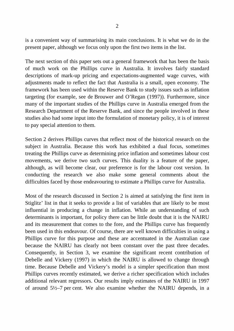
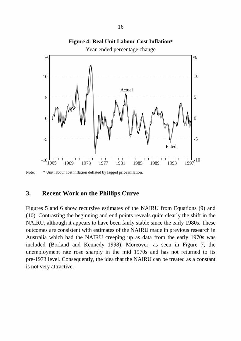
The 80.02 �R , 29.2�DW and the )4(2� test statistic for serial correlation is9.90 ( p-value = 0.04). The Jarque-Bera test for normality of the residuals has avalue of 14.85.12 The estimated NAIRU is 6.58 per cent with a standard error of0.81 per cent. Figure 4 shows the actual and fitted values of the dependent variablefrom this equation. Generally, the fit of the equation is quite good and tends to besuperior to that of the price equation. Given the history recounted earlier about thedifficulty of modelling wages, it is perhaps a little surprising that the equationworks so well compared with the price equation. One difference between our workand most of that in the past is that we model unit labour costs rather than wages.Since unit labour costs are relevant to pricing decisions, focusing on them seems areasonable strategy. Our use of a longer sample period than was available in earlierstudies may also be relevant since the wage-setting process has become lessregulated over time, especially in the 1990s.13
12 The Jarque-Bera test implies that this equation’s residuals are also non-normal. In contrast tothe price equation, however, this is caused by the influence of a few quarters of large rises inthe dependent variable (which coincide with large wage-case decisions) rather than thepresence of many small movements. Excluding these observations, normality of theunit-labour-cost residuals cannot be rejected.
13 One test of the importance of the longer sample period is to see how well the equationperforms over a sample finishing in 1973:Q1. The answer is that, in this regression, all of thevariables are insignificant apart from the wage inflation variables. We are, of course, onlyusing 31 observations in this regression and so no precision could be expected. By contrast,however, when the sample is restricted to the last 31 observations, all of the variables aresignificant, with the exception of the change in unemployment.
16
Figure 4: Real Unit Labour Cost Inflation*
Year-ended percentage change
-10
-5
0
5
10
-10
-5
0
5
10
1997
%
Fitted
Actual
%
19931989198519811977197319691965
Note: * Unit labour cost inflation deflated by lagged price inflation.
3. Recent Work on the Phillips Curve
Figures 5 and 6 show recursive estimates of the NAIRU from Equations (9) and(10). Contrasting the beginning and end points reveals quite clearly the shift in theNAIRU, although it appears to have been fairly stable since the early 1980s. Theseoutcomes are consistent with estimates of the NAIRU made in previous research inAustralia which had the NAIRU creeping up as data from the early 1970s wasincluded (Borland and Kennedy 1998). Moreover, as seen in Figure 7, theunemployment rate rose sharply in the mid 1970s and has not returned to itspre-1973 level. Consequently, the idea that the NAIRU can be treated as a constantis not very attractive.

17
Figure 5: NAIRU from the Price Phillips CurveDerived from recursive estimation
-4
-2
0
2
4
6
8
10
12
14
16
-4
-2
0
2
4
6
8
10
12
14
16
1997
% %
1993198919851981197719731969
Figure 6: NAIRU from the Unit Labour Cost Phillips CurveDerived from recursive estimation
-48
-40
-32
-24
-16
-8
0
8
16
24
-48
-40
-32
-24
-16
-8
0
8
16
24
112
120 120
112
19971993198919851977 198119731969
% %

18
Figure 7: Unemployment Rate
0
2
4
6
8
10
0
2
4
6
8
10
1997
% %
19931989198519811977197319691965
If one is to allow the NAIRU to shift over time, then the task becomes one offinding the best way to do that. In Phillips curve specifications such as thoseestimated earlier, the NAIRU is absorbed into the intercept, presenting thepossibility of using statistical procedures to determine the number and location ofbreaks in that coefficient. Once located, shifts in the NAIRU could be captured bya series of dummy variables. Early work on Treasury’s NIF-10 model of theAustralian economy did something like this, albeit in an informal way, and thecurrent Treasury macroeconomic model (TRYM) allows for a single shift in thelevel of the NAIRU in 1974.14
14 We formally tested for breaks in our Phillips curve relations, Equations (9) and (10), byapplying the battery of tests in Bai and Perron (1998). Generally, these tests suggest one ortwo breaks in each relation. For the price equation, the breaks are in 1972:Q4 and 1974:Q4.However, given how close these are to one another, it seems best to regard them as a singlebreak around 1973. For the wage equation, the most significant break identified was in1977:Q2 with a less significant break in 1973:Q4. Thus, the time pattern of the NAIRU

19
The logic of imposing breaks in the NAIRU based on an inspection of the historyof the unemployment rate follows from the observation that, within a few years ofa shock to the NAIRU, the unemployment rate adjusts back to this new equilibriumlevel in most macroeconomic models in use in Australia. In the TRYM model, forexample, this adjustment takes about three years (Downes and Stacey 1996) andthe outcome is similar in the class of models associated with Chris Murphy(Powell and Murphy 1997). Following a shock, the lengthy period of time duringwhich the two series have not converged, however, suggests that it may well bedifficult to derive reliable information about the (time-varying) level of the NAIRUsimply from the behaviour of the unemployment rate.
There is now an emerging literature (for example, Debelle and Laxton (1997) andthe references in Laxton et al (1998)) which involves treating the NAIRU as aunit-root process of the form:
ttt UU ��-
*1
* , (11)
where t is assumed to be ),0( 2n
N . The argument for a unit-root in the NAIRUis apparent from applying ‘unit-root accounting’ to both sides of Equation (6). Thedependent variable in that equation has little persistence; defining it as ty , anaugmented Dickey-Fuller-style regression of ty against 1-ty and jty �� , 41��j ,gives a coefficient on 1-ty of 0.53. Since most of the other variables are indifferenced form and tU behaves like a unit-root process (Appendix C), thissuggests that *
tU and tU must cointegrate. Of course, the variable 14* ln
-
��� tt PPis quite persistent (0.93 being the first-order term in the augmentedDickey-Fuller-style regression) and so we expect that this would also be true of thedifference *
tt UU � .
evident in the recursive estimates shown in Figures 5 and 6, seems to hold up to more formaltesting.

20
For Australia, Debelle and Vickery (1997) use a Phillips curve framework toestimate the NAIRU as a time-varying coefficient using the Kalman filter.15
Equation (12), which is a modified version of Equation (6), is Debelle andVickery’s preferred functional form for the price Phillips curve (to which we haveadded an error term t� that is assumed to be ),0( rN ).
� � � �t
t
ttttttt U
UUPPPPy ��� �
���������� ��
*
14*
144 lnlnln . (12)
This equation is a non-linear Phillips curve. Apart from appearing in both ofPhillips’ original papers (Phillips 1958, 1959) many other estimated AustralianPhillips curves have used this non-linear specification, e.g. all those associatedwith Murphy’s models and TRYM. Debelle and Vickery (1997) review thearguments for and against the non-linear Phillips curve specification.
As we have previously discussed, one might expect both import price andspeed-limit terms to appear in a price Phillips-curve relationship likeEquation (12). This suggests a richer specification, based on Equation (9) from theprevious section:
� �� � � � .lnlnlnln
)(lnlnln
41224141
1*
14*
144
����
���
�������
��
��
��������
tttt
t
t
t
tttttt
PPPMPM
U
Ud
U
UUPPPP
��
��(13)
We therefore estimate Equation (13) by maximum likelihood, assuming that theNAIRU evolves as a random walk, as in Equation (11).16 The coefficient estimates,
15 Given the fact that the Kalman filter does make some normality assumptions, and the changein inflation is clearly non-normal (Figure 2), one might wish to be cautious when interpretingthe results from this estimation.
16 Appendix D provides a discussion of some of the technical issues involved in this estimation.Two changes were made to the specification in Equation (9). One was to make the speed limitterm – the lagged change in unemployment – a ratio of the unemployment rate, in line with

21
and associated t-ratios (for the sample period 1966:Q1–1997:Q4) are:
.)52.1(566.0)89.13(470.0)40.11(705.0
)26.4(046.0)99.1(538.1)74.1(388.0)09.2(051.0
2
1
���
������
n�
���
r
d
These estimates imply that import prices make a very significant contribution tothe acceleration in inflation. Speed-limit effects, while less significant, also seemto contribute.17 One notable feature of the results is that the magnitude of � ismuch smaller than that found with Debelle and Vickery’s specification( 25.1��� ), i.e. the influence of deviations of the unemployment rate from theNAIRU upon the acceleration in inflation is much smaller. No doubt part of this isdue to the inclusion of the speed-limit term, but it is also due to the fact that otherregressors explain variations in inflation movements that were attributed to theNAIRU gap in Debelle and Vickery’s specification.
Figure 8 shows both one and two-sided estimates of the NAIRU fromEquation (13). For each period, the one-sided estimate is derived using data up toand including the previous period, while the two-sided estimate is based on datafrom the whole sample. As we would expect, both estimates of the NAIRU risesharply in the early 1970s. From the mid 1970s until the late 1980s, the estimatedNAIRU declines gradually, which may be explained, at least after 1983, as a
the non-linear structure of the Phillips curve. The second was to use the unemployment raterather than a moving average of it when defining the excess demand variable. As wasmentioned earlier, from the point of view of fit, it matters little whether one uses � �tU4MA
or tU as the measure of unemployment, and the former was preferred earlier because it
improves the shape of the implied lag distributions to a temporary shock. However, it wouldbe difficult to work with � �*
4MA tt UU � in the context of the Kalman filter. We also
estimated models in which the Phillips curve was linear in the unemployment rate but, basedon the values of the maximised log likelihoods, such models were always rejected in favour ofthe non-linear versions.
17 Debelle and Vickery (1997) also tested for speed-limit effects, but generally found them to beof the wrong sign (and insignificant). This result is presumably a consequence of the omissionof other relevant inflation explanators from their equation.

22
consequence of the Accord. By the early 1990s, however, the one-sided estimate ofthe NAIRU has fallen to an implausibly low level, although this problem is lessserious when the estimate is based on the whole sample. By the end of the sample,the estimate of the NAIRU is around 5½ per cent, although this estimate isimprecise.18
Figure 8: NAIRU from the Price Phillips Curve
One-sided NAIRU
Two-sidedNAIRU
0
2
4
6
8
0
2
4
6
8
1997
% %
1993198919851981197719731969
One-sided NAIRU
Two-sidedNAIRU
Note that, at a steady rate of both import-price and consumer-price inflation,Equation (13) implies that a steady unemployment rate will be equal to the NAIRUonly when inflation expectations, *
tP� , are equal to actual inflation, 14 ln-
� tP .Furthermore, while ever inflation expectations exceed actual inflation, a steadyunemployment rate must be above the NAIRU for actual inflation to remainsteady. These are general properties of all the Phillips curves we estimate in thispaper, and also of the Debelle-Vickery Phillips curve. This point is of empirical
18 The final estimate of the NAIRU is sensitive to the parameters � and n
. Since both are
estimated imprecisely, with t-ratios less than 2, the NAIRU is also estimated imprecisely.

23
relevance because our measure of inflation expectations exceeds actual inflationfor extended periods, with the gap averaging 2.1 per cent per annum over theperiod 1980–1997 (although it has disappeared by the end of the sample).
A similar analysis can be carried out by estimating a non-linear version of our unitlabour cost Phillips curve, Equation (10), augmented to allow for a time-varyingNAIRU:
� �� � � �,lnlnlnln
)(lnlnln
4122414
1*
14*
144
����
���
�������
��
��
��������
tttt
t
t
t
tttttt
ULCULCPULCc
U
Ud
U
UUPPPULC
�
��(14)
producing (for the sample period 1966:Q1–1997:Q4):
.)55.2(365.0)52.14(460.1)42.7(454.0
)76.11(666.0)68.1(372.4)01.2(868.1)02.2(132.0
2 ���
������
n�
��
r
cd
These estimates imply some role for speed-limit effects in the determination of unitlabour costs, as they did for the acceleration in price inflation. Figure 9 shows bothone and two-sided estimates of the NAIRU from this equation. Theunit-labour-cost Phillips curve appears to give a somewhat more plausible pictureof movements in the NAIRU than does the price Phillips curve, with much lessmovement in the estimates of the NAIRU since the mid 1970s. The dip in theunit-labour-cost NAIRU in the mid 1980s also appears more consistent with thetiming of the Accord. While there has been considerable debate over whether theAccord reduced the NAIRU, our evidence seems to suggest that it did – at least forsome time. At the end of the sample, the NAIRU is estimated to be around7 per cent, although this number is again estimated imprecisely.

24
Figure 9: NAIRU from the Unit Labour Cost Phillips Curve
0
2
4
6
8
0
2
4
6
8
1997
% %
1993198919851981197719731969
One-sided NAIRU
Two-sided NAIRU
Figure 10 presents a comparison of two-sided (that is, whole-sample) estimates ofthe NAIRU from our two preferred Phillips curves Equations (13) and (14) andfrom Debelle and Vickery’s price Phillips curve Equation (12). The time-profilesof these three estimated NAIRUs are fairly similar, suggesting that the addedcomplexity of our Phillips curve equations appears to add little to ourunderstanding of the evolution of the NAIRU.
There is, however, an advantage to our approach. Debelle and Vickery generate arelatively smooth time-profile for the NAIRU by imposing the assumption thatshocks to the NAIRU have a small variance (their key assumption is that theparameter q takes the value 0.4, where 22
n��q and 2
n is the variance of shocks
to the NAIRU). However, when the parameters in the Debelle-Vickery system are

25
freely estimated by maximum likelihood, q takes the value 7.1.19 Not surprisingly,the imposed value 4.0�q is clearly rejected by a likelihood ratio test.
Figure 10: Comparison of NAIRU Estimates% %
0
2
4
6
8
0
2
4
6
8
0
2
4
6
8
0
2
4
6
8
199719931989198519811973 19771969
Debelle-Vickery (1997)
Unit labour cost Phillips curve
Price Phillips curve
Notes: This figure shows estimates of the NAIRU based in each case on the whole sample of data
(two-sided estimates). The Debelle and Vickery (1997) results use their price Phillips curve
specification and their methodology estimated over our sample period (1966:Q1–1997:Q4).
The results generated by maximum-likelihood estimation of the Debelle-Vickerysystem are, however, unsatisfactory because they imply an unrealistically volatileprofile for the NAIRU, with values ranging from less than zero to more than20 per cent over the sample (results not shown). By contrast, the extra terms in ourmore complex specifications explain much of the variation in inflation that mustinstead be attributed to the unemployment gap in the Debelle-Vickeryspecification. As a consequence, we generate smooth (maximum-likelihood)
19 Other parameters also take different values, but the value of q is the key difference.

26
estimates of the time-profile of the NAIRU without the need to impose restrictionson the parameters which are rejected by the data.
We now examine the stability of our time-varying models of the NAIRU, focusingon our preferred unit labour cost Phillips curve model Equation (14). The results ofrecursively estimating the parameters in that model are shown in Figure 11, wherethe coefficients on the following variables are plotted: 14
* ln-
��� tt PP (anticipatedinflation), ttt UUU )( *� (proportional NAIRU gap), tt UU 1-� (change inunemployment) and 41 lnln
--
��� tt ULCULC (lags of quarterly unit labour costinflation). The coefficient on the lagged dependent variable is extremely stable,and so is omitted from the figure. The difficulties that any wage or price equation
Figure 11: Parameter Estimates from the Unit Labour Cost Phillips CurveDerived from recursive estimation
-8
-6
-4
-2
0
2
4
-8
-6
-4
-2
0
2
4
-8
-6
-4
-2
0
2
4
-8
-6
-4
-2
0
2
4
0.00.20.40.60.81.01.2
0.00.20.40.60.81.01.2
199719941991
Proportional NAIRU gap
Change in unemployment
Anticipated inflation
Lags of quarterly unit labour cost inflation
1988198519821979197619731970

27
faces with data from the early 1970s are very clear, but the equation seemsreasonably stable apart from that.20
While treating the NAIRU as a stochastically time-varying coefficient is a usefulapproach, there are other ways to deal with the fact that the NAIRU isunobservable. For example, it is often of considerable interest to know whetherunemployment is above or below the NAIRU, without being so concerned about itsdistance from the NAIRU. One way to determine this is to treat )( *
tt UU �� inEquation (6) as a latent variable t� , and to estimate an equation of the form:
� � ttttt PPPP �� ��������-- 14
*144 lnlnln . (15)
The question then becomes one of how to model the latent variable t� . Onestrategy is to treat it in the same way as Hamilton (1989) and assume that itinvolves two states, with the draws in each state coming from different normaldensities ),( 11 N and ),( 22 N .21 Transition probabilities then govern themovement from one state to another. Applying this methodology to the pricePhillips curve Equation (13), and replacing ttt UUU )( *�� with a two-state latentvariable, the resulting parameter estimates, for the sample period1966:Q1–1997:Q4, are:
.)78.12(759.0)22.4(034.0)68.2(260.2)04.2(030.0 21 ����� ��� d
The signs of the estimated values of 1 and 2 are different, with 1 beingpositive. Since � is expected to be negative, this sign suggests that the first stateoccurs when unemployment is below the NAIRU. Figure 12 shows the estimatedprobability of being in this state (below the NAIRU). In the same figure we alsoshow the proportional NAIRU gap ttt UUU )( *� estimated from the price Phillips
20 An alternative approach for testing the structural stability of the equation is to apply the testsdescribed in Bai and Perron (1998). These tests suggest that there may be a structural break,although their sequential test suggests no break.
21 Another would be to allow the gap between the unemployment rate and the NAIRU to evolveas an autoregressive process.

28
curve Equation (13). Figure 12 confirms what has long been believed, that the late1960s and early 1970s were periods when the economy was below the NAIRU,but, apart from a period at the beginning of the 1980s, the Australian economy hassince been above the NAIRU.
Figure 12: Measures of Excess Labour Demand
-1.2
-1.0
-0.8
-0.6
-0.4
-0.2
0.0
0.2
0.4
0.6
0.8
1.0
1997199319891985198119771973
Probability of being below the NAIRU (LHS)
Proportional NAIRU gap from pricePhillips curve (RHS)
1969
0
%
100
80
60
40
20
Making the NAIRU a strictly exogenous variable as in Equation (11) means thatOLS can be applied under the same conditions as when the NAIRU is assumedfixed.22 However, as there has been a great deal of debate over determinants of the
22 A stochastically varying NAIRU also makes it computationally difficult to treat theunemployment rate as an endogenous variable in a (possibly) non-recursive system. Thus thetype of analysis conducted by King and Watson (1994) is difficult to perform unless oneconditions upon estimates of the NAIRU, but doing so fixes one of the equations of thesystem.

29
NAIRU, it seems worthwhile to experiment with some modifications toEquation (11). Specifically, we estimate models of the form:
ttttt fafaUU �������- 2211
*1
* , (16)
where the factors tf1 and tf2 are taken to be I(1) and are therefore entered indifferenced form. Two I(1) variables which are thought to influence the NAIRUare the replacement ratio and the long-term unemployment rate (Figure 13). Thelatter is taken to represent ‘hysteresis’ effects. After jointly estimatingEquation (14) with the augmented specification for the NAIRU in Equation (16),the coefficients 1a and 2a are found to be neither statistically nor economicallysignificant. Other experiments in which the factors were taken to be the laggedvalues of the unemployment rate itself produced the same conclusion.
Our inability to explain changes in the NAIRU using either the replacement ratioor the long-term unemployment rate, while disappointing, accords withinternational studies which have also found it difficult to explain differences inunemployment rates between countries and across time on the basis of a smallnumber of measurable, causal factors (Jackman 1998).
Figure 13: Long-term Unemployment and the Replacement Ratio
0
1
2
3
4
0
10
20
30
40
Replacement ratio (RHS)
19971989 1993198519811977197319691965
%
Long-term unemployment rate (LHS)
%

30
4. The Phillips Curve and Monetary Policy
The Phillips curve is clearly a useful empirical device for examining thedeterminants of inflation in Australia. It also, however, provides an intellectualframework for the analysis of monetary policy. In this section, we discuss theintellectual development of the Phillips curve framework within the Reserve Bankof Australia, and particularly within its Research Department. This is of particularinterest because many of the Australian empirical studies of the Phillips curvecame from this part of the Reserve Bank. It also seems likely that the ideasformulated in this research would have had an influence, perhaps after some time,on the formulation of monetary policy in Australia.
In earlier sections of this paper we showed how conceptions of the Phillips curveand its determinants in Australia had changed over the past three decades and so itis useful to look at monetary policy developments in the light of the results that wehave established. In the 1960s, the policy framework in Australia, as in mostcountries, almost certainly accepted the unemployment/inflation trade-off implicitin the first generation of Phillips curves. Nevertheless, strong economic growth atthe time meant that the perceived trade-off did not need to be exploited. In the lastyear of that decade, the Reserve Bank began issuing research discussion papers,and among the crop of seven papers produced in that year was one titled ‘AnEquation for Average Weekly Earnings’, by K.E. Schott. This paper was part of aproject within the Reserve Bank to construct a macroeconometric model of theAustralian economy, which was released in its initial form in January 1970, andbecame known as the RBI model (Norton 1970). The Schott paper refers toPhillips’ (1958) original Economica paper, but makes no reference to either thePhelps (1968) or Friedman (1968) papers, which introduced the idea that there wasno long-run trade-off between inflation and unemployment. Given this omission, itis perhaps not surprising that the econometric results presented by Schott impliedthe existence of a trade-off between inflation and unemployment in the long-run,although this implication is not drawn out in the paper.
With the dawning of the 1970s, and the rapid acceleration of inflation in Australia,the question of whether there was a long-run trade-off became one of greaterurgency. In mid 1971, the Head of Research Department, Austin Holmes, wrote aninternal paper on the problems of inflation which made a clear statement about the

31
distinction between the short-run and long-run trade-offs between inflation andunemployment:
Inflationary expectations can help to explain the differences over time in the apparenttrade-off between wage rises (and the rate of inflation) and the rate ofunemployment. Empirical studies linking these two have often found that therelationship is improved if the recent rate of increase in prices (a proxy forexpectations) is included. If, as seems likely, wage claims are specified in real terms,the interpretation of Phillips’ curves becomes somewhat clouded. They can rule onlyfor a given set of expectations about prices. Changes in these expectations lead toequivalent changes in the rate of increase in wages for a given level ofunemployment.
(Research Department 1971, p. 4)
Much of the analysis contained in this ‘Inflation’ paper remains of interest in thelate 1990s. In a later section, the paper argues that inflationary expectations, onceraised, might prove hard to reduce. It canvasses the possibility that expectationsmight not respond to announcements of the anti-inflation resolve of the authorities,and might be difficult to lower without a period of higher unemployment. Giventheir contemporary relevance, it is worth quoting these arguments at some length.
Suppose an economy has proceeded for some time with activity high and inflationpositive but moderate. Expectations of future growth in prices have been formed.
Suppose this situation is disturbed by an upsurge in demand resulting from, say, anexport or investment boom. Does this require only an application of traditional fiscaland monetary measures to reduce demand? And, after the faster price rises generatedby the excess expenditure have worked their way through the economy (this could,of course, take some time), can the economy return to its previous acceptable patternof activity and price performance? This seems to depend a good deal on what hashappened to expectations about prices.
Where inflationary expectations are unaffected by these hypothetical developments(our knowledge about what actually affects these expectations is far from perfect),the economy can resume its previous pattern. However, if the episode leads to, say,an upward revision in the community’s expectations about inflation, the answersseem to change somewhat. It is assumed, of course, that the revised expectationspersist in the face of pronouncements of concern by the authorities and even of theannouncement and effects of the fiscal and monetary measures.
In this situation, there is a rise in the economy’s aggregate supply schedule. Withdemand given, this would lead to a lower level of activity but a faster rate of increasein prices than previously. Attempts to restore activity lead to even faster growth inprices. In other words, following a change in inflationary expectations, the fiscal andmonetary policies consistent with a given level of employment have to be moreexpansive than before the change.

32
It does not require a burst of demand to induce the change in expectations. Thiscould result from a sudden awareness that, say, previous expectations about stableprices ought to be abandoned in the face of x years of positive price increase. Perhapsthe inflationary expectations can be imported. Whatever the cause, a return to pricestability with high employment requires a change in price expectations. If these arefirmly entrenched, as they might be if a fairly long history of price increases figuresin their formation, one cannot be too optimistic about the ability of fiscal andmonetary measures to do this without a period of higher unemployment.
(Research Department 1971, p. 6)
It was not too long before empirical support for the arguments set out in the‘Inflation’ paper was provided by econometric evidence from the Australianeconomy. In a Reserve Bank Research Discussion Paper issued in August 1973,Jonson, Mahar and Thompson estimated several equations for the annual growth inaverage weekly earnings. As well as variables capturing demand effects, theequations included growth in award wages and in world prices as explanators. Intheir preferred equation, the sum of the coefficients on the ‘price’ terms wasinsignificantly different from one, from which the implication was drawn that therewas no long-run trade-off between the rate of inflation and the state of the labourmarket in Australia. This preferred equation for average weekly earnings, as wellas an equation for award wages, were soon incorporated into the Bank’s RBImacroeconometric model with only minor amendments.
Professor Michael Parkin, a visitor to the Bank at the time, seems to have playedan influential role within the Research Department by providing a unifyinginterpretation of the available econometric evidence. Jonson, Mahar andThompson (1973) credit Parkin with pointing out that their empirical resultsimplied the absence of a long-run inflation-unemployment trade-off.Furthermore, the Jonson, Mahar and Thompson paper was a revised version of apaper by Jonson and Mahar, issued in November 1972, which contained much thesame econometric exercise as the later paper (using a slightly shorter sample), butdid not draw any implications from the results about the long-runinflation-unemployment trade-off.
Parkin also produced a research paper on ‘The Short-run and Long-run Trade-offsbetween Inflation and Unemployment in Australia’ in the second half of 1973, inwhich he presented a critical analysis of the long-run inflation-unemploymenttrade-offs implied by several recent econometric studies of wage and price

33
inflation in Australia. On both theoretical and empirical grounds, he argued thatthose studies which implied a non-zero long-run trade-off were flawed. His paperled to a series of responses and rebuttals in the pages of Australian EconomicPapers that continued for several years.23
Of course, the intellectual framework for analysing the inflationary process wasnot the only thing that was changing around this time. The economic landscapewas also changing. As well as the rapid deterioration in the inflation performance(Figure 14), it is now clear that the NAIRU in Australia also rose significantly inthe early 1970s.24
Figure 14: Underlying Inflation and Inflation Expectations
0
5
10
15
20
0
5
10
15
20
0
5
10
15
20
0
5
10
15
20
Underlying inflation
Bond yields
Melbourne Institute inflationexpectations (median)
Indexed bonds
199719931989198519771973 198119691965
% %
23 See, for example, Challen and Hagger (1975), McDonald (1975), Nevile (1975),Parkin (1976) and Rao (1977). Hagger (1978) later reviewed the debate at length.
24 The rapid deterioration in inflation is consistent with our earlier empirical finding that theunemployment rate was below the NAIRU for much of the decade 1966–75 (see theproportional NAIRU gap in Figure 12). The significant rise in the NAIRU is clear from boththe price and unit labour cost Phillips curves (Figures 8 and 9).

34
For the Phillips-curve framework to be useful as a guide for monetary policy, itwas of course necessary to have some reasonable idea of the level of the NAIRU –in order to be able to assess the inflationary implications of any given rate ofunemployment.25 While we would now date the beginning of the significant rise inthe NAIRU somewhere around 1970–1972 (based on both the price and unit labourcost Phillips curves in Figures 8 and 9), this rise was far from clear at the time. Forexample, in the paper discussed above, Parkin (1973) argued that the naturalunemployment rate had probably fallen since the early 1960s, to be in the 1½ to2 per cent range at the time of writing in late 1973.
By early 1976, however, the then Head of the Research Department, W.E. Norton,argued in a published paper that recent experience in several countries (includingAustralia) suggested that the NAIRU (which he called ‘the lowest sustainable rateof unemployment’) seemed to have increased, although he offered no quantitativeestimate of the extent of the increase (Norton 1976).
The difficulties inherent in coming to a view about the level of the NAIRU in themid 1970s probably also made some contribution towards another importantchange in the Reserve Bank’s thinking about the inflationary process. As with theintroduction of the idea that the long-run Phillips curve was vertical, this changealso owed a large debt to intellectual developments overseas.
In the 1971 ‘Inflation’ paper, the causes of inflation were discussed under thesubheadings: labour costs, material costs (including, importantly, the price ofimported goods), taxes and profits. The paper argued that inflation was caused byboth excess demand and adverse supply shocks. Excess demand led to higherinflation primarily because of rising labour costs (although firms’ mark-ups oncosts might also rise) as the economy travelled up a short-run Phillips curve. Theresult was higher inflation – rather than a once-off rise in the price level – becauseinflationary expectations were disturbed. In light of later developments, it is of
25 Wieland (1998) provides a modern discussion of the optimal interplay between policygradualism and experimentation when there is uncertainty about the level of the NAIRU.

35
interest to note that the paper did not discuss excess money growth as one of thecauses of inflation.
Quite soon after the ‘Inflation’ paper was penned, however, monetary growthbegan to play a more prominent role in explanations of the inflationary processwithin the Research Department. Jonson, in an internal paper written in October1973, put the argument in these terms:
…our positive knowledge of the workings of the economic system establishes ageneral presumption that if we desire to control inflation we should carry out anystabilization policy within the constraint of an average rate of growth of the moneystock determined by the growth of ‘full employment’ demand at current inflationrates.
(Jonson 1973, p. 4)
In common with developments overseas, money came to play a central role in thesecond half of the 1970s, both in macroeconometric models developed within theBank, as well as in the formulation of Australian monetary policy itself. A secondgeneration of macroeconometric models (called RBII) developed within theResearch Department appeared in a series of versions during the second half of the1970s, and well into the 1980s (the last Research Discussion Paper to use RBIIwas written in 1987). Money had a key role in this generation of models, withseveral transmission channels through which money growth had a direct andimmediate influence on both real and nominal magnitudes within the economy,including, in particular, both wage and inflation outcomes.
In the formulation of Australian monetary policy, money growth became anintermediate target in 1976, when the Government began announcing an annualprojection for growth in the broad monetary aggregate, M3. This practice wasmaintained, with only slight variations, until early 1985 when, faced with evidence

36
of a breakdown in the empirical relationship between growth in M3, nominalincome and interest rates, the Government abandoned the M3 projection.26
In principle, analysis of the inflationary process based on a Phillips curveframework, with allowance made for open-economy aspects and supply shocks,could exist along side an analysis based on money growth. The two intellectualframeworks need not be seen as incompatible. To the extent, however, that excessmonetary growth was seen at the time as the fundamental cause of inflation, it wasnatural that a framework that highlighted the importance of controlling moneygrowth would gain pre-eminence over one that focused on the demand/supplybalance in the markets for labour and goods.
With the end of money-growth targeting in Australia, there was a transition periodfor monetary policy, in which policies became more pragmatic and there was asearch for alternative guiding principles. For a time, there was a policy ‘checklist’,which was a range of variables, which were to be consulted in assessing economicconditions and making policy decisions. An early description of the checklistapproach by Governor Johnston makes clear the very wide range of variables thatwere considered relevant. They included:
…all the monetary aggregates; interest rates; the exchange rate; the externalaccounts; the current performance and outlook for the economy, includingmovements in asset prices, inflation, the outlook for inflation and marketexpectations for inflation.
(Johnston 1985, p. 812)
The checklist was essentially an amalgam of instruments, intermediate and finalpolicy objectives, and general macroeconomic indicators. Although thedemand/supply balance in the labour and goods markets would undoubtedly havebeen considered relevant elements of the checklist, the Phillips curve certainly didnot play a central role in this view of the inflationary process.
26 See Argy, Brennan and Stevens (1990) for a comparison of the monetary targeting experienceof Australia and other countries.

37
In the late 1980s and into the 1990s, the framework for monetary policy evolvedgradually. A medium-term inflation target formed the centrepiece of theframework from around 1993, although many of its essential elements were inplace several years earlier.27 A monetary policy framework with a medium-termfocus on inflation as the policy objective, no intermediate objective, the short-terminterest rate as the instrument, and a transmission process that works via the effectof interest rates on private demand, had been analysed in several pieces publishedby the Bank in 1989, including its conference volume.28
In many ways, the intellectual framework for analysing the inflationary processwithin the Reserve Bank has come full circle. The framework of the 1990s hasmuch in common with the one enunciated in the ‘Inflation’ paper written in 1971,although the modern version would perhaps contain a few elements not present inthe earlier version. These are the main elements of the modern version.
In the short-run, output above potential (or, equivalently, unemployment below theNAIRU) generates rising wage growth and, perhaps, increases in firms’ mark-ups,which in turn, feed into inflation. Speed-limit effects are also relevant, so thatstrong output growth (or rapidly declining unemployment) also generatesinflationary pressures.29
Inflationary expectations are central to the inflationary process; the Phillips curveis indeed of the expectations-augmented variety, so that there is no trade-offbetween inflation and unemployment in the long-run. Inflationary expectationsseem relatively immune to announcements of the authorities’ anti-inflation resolve.
27 The numerical objective of 2–3 per cent underlying inflation began appearing in publicstatements by Governor Fraser in 1992 and 1993. International organisations (for example,the Bank for International Settlements) date the adoption of the Australian inflation targetfrom 1993. Grenville (1997) discusses the history of the inflation target in more detail.
28 See Macfarlane and Stevens (1989), Macfarlane (1989) and Grenville (1989).29 Recall that speed-limit effects are present in both the price and unit labour cost Phillips curves
presented earlier. The Bank’s 1995 Annual Report also drew attention to them:‘…unemployment remains well above the point at which serious inflationary pressures arelikely to be experienced. The relatively rapid speed of its fall over the past two years,however, has been such as to prompt a pick-up in labour costs’ (p. 15).

38
To achieve a sustained reduction in inflation and inflationary expectations, itappears to be necessary to run the economy for a period with output belowpotential and unemployment above the NAIRU. Furthermore, inflationaryexpectations take a long time to fully adjust to a fall in the trend rate of inflation –especially after an extended period of high inflation. Thus, for example, thetransition to low inflation in Australia was complete by 1992. Nevertheless,while inflationary expectations both in the bond market and among consumers fellto some extent at that time, the fall in inflationary expectations in the bond marketdid not fully reflect the lower trend rate of inflation until 1997, and even then,consumers’ inflationary expectations appeared not to have fully adjusted to thelower trend rate of inflation (Figure 14).
Open-economy aspects are also important to the inflationary process. A fall in theexchange rate, triggered, for example, by a fall in the world price of Australiancommodity exports, leads to a rise in import prices, which feeds into consumerprices with a lag. Whether a once-off fall in the real exchange rate translates into arise in the rate of consumer inflation (rather than simply a once-off rise in the levelof consumer prices) depends on whether inflationary expectations are disturbed.This is an empirical issue; there should not, however, be an automatic presumptionthat inflationary expectations are immune to such an exchange-rate-induced rise inconsumer prices.
The rate of money (or credit) growth is an important indicator of the pace offinancial intermediation in the economy. Money growth does not, however, havean independent effect on either activity or inflationary expectations in theeconomy, once the effects of the level of real interest rates and asset prices,including the exchange rate, have been allowed for.
5. Conclusion
In this paper, we have examined the history of the Phillips curve in Australia inthe forty years since Phillips first estimated one using Australian data. We focusedon the changing perspectives of researchers trying to estimate Australian Phillipscurves, as well as on the fluctuating fortunes of the Phillips curve in the intellectualframework used to analyse inflation in Australia within the Reserve Bank.

39
Several themes stand out from this history. First, from Phillips (1959) onwards,researchers estimating Australian Phillips curves have had to deal with the uniqueinstitutional features of the Australian labour market, particularly in the era whenthe Arbitration Court set both award and minimum wages. As a consequence of theCourt’s role in that era, it has been particularly difficult to model the evolution ofwages in Australia without taking explicit account of arbitrated movements inaward wages.
A second important theme is the crucial role of inflation expectations in thePhillips curve framework. Here the Australian experience mirrors that of othercountries. In the 1960s, there was a widespread assumption, implicit or explicit,that in response to a change in the trend rate of inflation, inflationary expectationseither did not adjust, or adjusted only incompletely. As a consequence, there was apresumed trade-off between inflation and unemployment, even in the long run.
With the deterioration of the inflationary performance in the early 1970s, however,this presumption was challenged, by Austin Holmes in an internal Reserve Bankpaper written in 1971, and by Michael Parkin in an academic paper written whilehe was visiting the Reserve Bank in 1973. In the aftermath of these papers (whichdrew their inspiration from the 1968 papers of Friedman and Phelps) the idea of along-run trade-off between inflation and unemployment was soon discredited.
A third recurring theme in the history of the Australian Phillips curve concerns thedifficulties posed by the changing level of the non-accelerating inflation rate ofunemployment (NAIRU). While it is now clear that the NAIRU was rising rapidlyin the early 1970s, this was far from obvious at the time – with Parkin even arguingthat it may have fallen since the early 1960s, to be in the range 1½–2 per cent bylate 1973. It was not until a few years after 1973 that analysts became confidentthat the NAIRU had indeed risen significantly.
One response to this problem by researchers estimating Phillips curves had been tosimply impose a structural break in the level of the NAIRU, on the basis of anexamination of the history of the unemployment rate. An alternative response,introduced into the Australian literature by Debelle and Vickery (1997) and alsoadopted in this paper, was to estimate the Phillips curve in conjunction with anequation that allows the NAIRU to evolve through time.

40
Using this approach, we estimated Phillips curves for both prices and unit labourcosts in Australia over the past three decades. These Phillips curves suggest a rolefor both the level of unemployment and its rate of change (‘speed-limit’ effects) inthe determination of inflation outcomes. Our results imply that the NAIRU inAustralia rose from around 2 per cent in the late 1960s to around 6 per cent in themid 1970s. Since then, the NAIRU was estimated to have dipped slightly in themid 1980s, before rising slightly to be around 5½–7 per cent at the end of oursample in 1997.
The difficulty of assessing the actual level of the NAIRU in the early 1970s alsoplayed a part in a final theme in the history of the Phillips curve in Australia: itschanging influence in the intellectual framework used to analyse inflation withinthe Reserve Bank.
An expectations-augmented version of the Phillips curve had formed thecentrepiece of the analysis presented by Austin Holmes in his 1971 internal paper,‘Inflation’. This centrepiece was not of much use, however, if one had very littleidea about the actual level of the NAIRU, which left the way open for otherexplanations of the inflationary process to gain prominence. In particular, thosebased on excess money growth were becoming influential around the developedworld. As in other countries, this confluence of events led to a downplaying of theimportance of the Phillips curve in the framework used to analyse inflation in theReserve Bank, and an increase in the focus on money growth.
From the mid 1970s to the mid 1980s, money growth remained at centre-stage,both as an intermediate target for monetary policy, and in the modelling of theinflationary process in the Reserve Bank. With the end of money-growth targeting,a transition period followed, in which the framework for monetary policy graduallyevolved.
By the 1990s, however, the intellectual framework for analysing inflation hadcome full circle. The framework of the 1990s had much in common with the oneenunciated in the 1971 ‘Inflation’ paper. The intervening years had led to somerefinement of the analysis, but the expectations-augmented Phillips curve hadreturned and once again was at centre-stage.

41
Appendix A: National Wage Case Outcomes (1968–1981)
Date at which NationalWage Case becameoperative
Award wage ratesincreased by
Minimum wageincreased by
Percentage change inAWE over thefollowing year
December 1968 $1.35 $1.35 (3.5%) 7.1
December 1969 3.0% $3.50 (9.0%) 8.7
January 1971 6.0% $4.00 (9.5%) 7.3
May 1972 $2.00 $4.70 (10.0%) 11.8
May 1973 2.0% plus $2.50 $9.00 (17.5%) 20.8
May 1974 2.0% plus $2.50 $8.00 (13.0%) 22.8
December 1974(a) $8.00 (12.0%)
May 1975 3.6% $4.00 (5.0%) 16.7
September 1975 3.5% $2.80 (3.5%) 16.1
February 1976 6.4% 6.4% 13.1
April 1976(a) $5.00 (5.5%)
May 1976 3.0% for awards to$125/wk then flat $3.80
3.0% 10.8
August 1976 $2.50 for awards to$166/wk then 1.5%
$2.50 (2.5%) 9.7
November 1976 2.2% 2.2% 10.0
March 1977 $5.70 $5.70 (5.5%) 10.5
May 1977 1.9% for awards to$200/wk then flat $3.80
1.9% 8.6
August 1977 2.0% 2.0% 9.1
December 1977 1.5% 1.5% 7.2
February 1978 1.5% for awards to$170/wk then flat $2.60
1.5% 8.8
June 1978 1.3% 1.3% 6.9
December 1978 4.0% 4.0% 9.9
June 1979 3.2% 3.2% 11.6
January 1980 4.5% 4.5% 12.9
July 1980 4.2% 4.2% 10.8
January 1981 3.7% 3.7% 13.8
May 1981 3.6% 3.6% 14.0
Note: (a) Minimum wage decision only.
Sources: Australian Economic Review, various issues, 1968–1981.
ACTU Living Wage Case Submission, November 1996, Section B, pp. 78–81.

42
Appendix B: Exogeneity Assumptions Relevant to EstimatingPhillips Curves
As the Phillips curve is a single equation in a system, estimating Equations (6) and(8) in Section 2 means that some exogeneity assumptions must be invoked. Inmany recursive vector autoregression (VAR) studies, prices are ordered afteroutput, implying that the latter is weakly exogenous in the price equation. Forexamples, see the US studies by Sims (1980) and Leeper and Gordon (1992).Australian VAR research has also continued this tradition, as seen in the work bySmith and Murphy (1994) and Dungey and Pagan (1997). The logic behind thisordering comes from the perceived short-run rigidity of prices and the role ofinventories in facilitating a de-coupling of prices and output in the short run.Moreover, when unemployment appears as the variable affecting prices, theargument for weak exogeneity is even stronger because movements in theunemployment rate are generally regarded as lagging output. In any case, someidentification assumption needs to be invoked and Phillips curve research inAustralia has invariably chosen the identification assumption we have justdescribed.
A further consideration is that the forward-looking component of inflationexpectations may be correlated with the error term in the price equation if theinformation set which agents use to forecast inflation is much broader than thatformed from the past history of inflation and the contemporaneous and lagged gapsbetween the unemployment rate and the NAIRU. For example, this may be thecase in Equation (6) since it is well known that import prices are useful forforecasting inflation in Australia. This is, however, only an argument forexpanding the specification of Equation (6), which we do in the paper. The crucialassumption in Equation (6) is that expectations of inflation are formed beforeprices are determined.

43
Appendix C: Time-series Properties of the Variables
Variable DF teststatistic(a)
Order of ADFtest(b)
ADF teststatistic(c)
�̂ from ADFtest
144 lnln-
��� tt PP -6.108* 4 -4.437* 0.525
14* ln
-
��� tt PP -1.793 1 -2.703 0.932
tU -1.238 4 -1.439 0.988
144 lnln-
��� tt PULC -3.797* 4 -3.480* 0.761
144 lnln-
��� tt PMPM -11.002* 3 -8.929* -0.379
Notes: * Denotes significance at the 5 per cent level using critical values from Fuller (1976). The tests were
conducted over the sample period 1965:Q1–1997Q4.
(a) This is the t-ratio on (��–1) in the Dickey-Fuller (DF) regression:
.)1( 1 ttt yy ��� �����-
(b) The order of the augmented Dickey-Fuller (ADF) test was determined by maximising the Schwarz
Bayesian Criterion.
(c) This is the t-ratio on (��–1) in the ADF regression ( j is the order of the ADF test):
.)1( 1 tj
jttt yyy ��� ������� �--
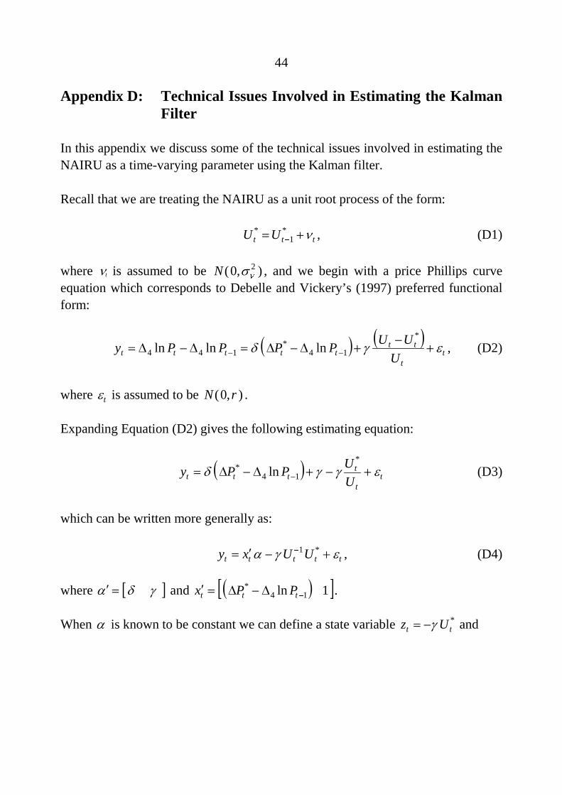
44
Appendix D: Technical Issues Involved in Estimating the KalmanFilter
In this appendix we discuss some of the technical issues involved in estimating theNAIRU as a time-varying parameter using the Kalman filter.
Recall that we are treating the NAIRU as a unit root process of the form:
ttt UU ��-
*1
* , (D1)
where t is assumed to be ),0( 2n
N , and we begin with a price Phillips curveequation which corresponds to Debelle and Vickery’s (1997) preferred functionalform:
� � � �t
t
ttttttt U
UUPPPPy ��� �
���������� ��
*
14*
144 lnlnln , (D2)
where t� is assumed to be ),0( rN .
Expanding Equation (D2) gives the following estimating equation:
� � tt
tttt U
UPPy ���� ������� �
*
14* ln (D3)
which can be written more generally as:
ttttt UUxy ��� ��� - *1 , (D4)
where ���� � and � � �1ln 14*
-
���� ttt PPx .
When � is known to be constant we can define a state variable *tt Uz ��� and

45
then Equations (D1) and (D2) constitute a state space form (SSF):
ttttt zHxy �� ��� (D5)
ttt zz ���-1 , (D6)
where 1-� tt UH , tt v�� �� , � � 2)var(n
�� �� qt and rt �)var(� .
Because of the ability to represent the equations as a SSF, most researchers usingthis approach to account for a time-varying NAIRU have estimated the state tz ,conditional upon the past history of ty (and contemporaneous tx ), with theprediction segment of the Kalman filter. This produces )(1 tt zE
-
. To do that it isnecessary to initiate the recursion with an initial value for the state 0|1z and itsvariance 0|1P . In most instances 0|1z is treated as a parameter and 0|1P is set to zero(Pagan 1980). Subsequently, conditional upon the values of r,
n and 0|1z one can
derive the innovations )(1 tttt yEy-
��� and their conditional variances th ,whereupon the log likelihood will be:
� �����t
tt h
hn
L2
2
1)(log
2
1)2(log
2
�� . (D7)
Maximising Equation (D7) then provides a way of estimating any unknownparameters.30
One of the most important parameters to be estimated is q . Apart from fixing it, asDebelle and Vickery do, there have been other suggestions in the literature.Laxton et al (1998, p. 29) report setting rq � when using annual data, because theresulting estimates of the NAIRU were not excessively volatile. This suggests thatone needs to study the impact of varying q more carefully in order to understand
30 Debelle and Vickery (1997) do not proceed in this way. Instead, they set r = 1, pre-specify
0|1z and 0|1P , and then seem to determine q by how well the resulting estimated path of the
NAIRU accords with their priors. Thus, the role of data in determining their NAIRU estimatesis more limited than it need be.

46
exactly how the estimates of the NAIRU are made. To do so, it is best toconcentrate � and 0|1z out of the likelihood, leaving only r and q as parameters.The key to doing this is to examine the Kalman prediction equations. One canshow that the prediction of the state *
tt Uz ��� using past information is:
)(1||1 �tttttttt xyKzbz ��� �� , (D8)
where 11|1| )( �
�� �� rHPHHPK tttttttt is the gain of the Kalman filter, 1| �ttP is thevariance of tz conditional on past information (a quantity that is computed by theKalman filter algorithm and depends only on r and q ) and ttt KHb ��1 .Recursively solving Equation (D8) gives:
�� xtytttt sszz ���� 0|11| , (D9)
where
1�� jjj b �� (D10)
111 ��� �� jjyjjyj yKsbs (D11)
111 ��� �� jjxjjxj xKsbs (D12)
are also generated recursively for nj �1� using initial conditions 11 �� , 01 �ysand 01 �xs .
With this information, the innovations )(1 tttt yEy-
��� can be written as:
)( 0|1 ���� xtytttttt sszHxy ����� . (D13)
Since the maximum likelihood estimates of � and 0|1z maximise Equation (D7) itis clear that, for a given r and q , they can be estimated by performing a weightedleast squares regression of yttt sHy � against xttt sHx � and ttH � , where theweights are the inverse of the standard deviation of the innovations (their estimatedvariance th depends only on r and q ). Thus we can easily concentrate � and 0|1zout of the log likelihood, leaving only r and q .

47
The result just described is useful for producing graphical representations of thesensitivity of the log likelihood to variations in q as well as helping us tounderstand how the NAIRU is estimated. Equation (D8) shows that the estimate ofthe state tz is a weighted average of all past values of �tt xy � with weights thatdecline like tb but which also vary with tK . If a linear version of the Phillips curvehad been used, tH would not vary with time, and one could have used theasymptotic version of the Kalman filter; this results in a constant gain K and,hence, constant weights b . In that case one would simply be doing a geometricallyweighted average of the residuals �tt xy � when forming the estimated tz . Toderive an estimate of the NAIRU from tz one also needs to divide by the estimateof � . This analysis points to the fact that estimates of the NAIRU made using thismethodology will depend upon the ability of tx to predict the change in inflation
ty , and not just on r and q . Moreover, the NAIRU is very sensitive to theestimate made of � . In this respect, the problems of getting a precise estimate ofthe time-varying NAIRU are the same as with the constant-NAIRU version in anequation such as Equation (9), where the intercept in the regression is dividedby � . All that happens now is that the numerator is replaced by a weighted averageof some residuals rather than an estimated intercept. The explicit formula inEquation (D8) could be useful for those papers looking at monetary policy in theface of a changing NAIRU, for example, Wieland (1998), where the authoritiesneed to solve a signal extraction problem when devising an optimal policy.
An important message from this analysis is that close attention needs to be paid todevising a suitable specification for the equation linking ty and tx . For this reasonEquation (9), from Section 2, seems a suitable source of extra regressors in tx overand above those used by Debelle and Vickery (1997). Such an extension producesthe specification for the price Phillips Curve Equation (13), which we estimate inSection 3. Parameter estimates (and the associated t-ratios) for that equation arepresented in the text. Here we examine the sensitivity of the log likelihood tovariations in r and q using the technique just described. Figure D1 shows a threedimensional plot of the concentrated log-likelihood function against values of rand q . This figure shows that we could accept a wide range of hypotheses aboutvalues of q , which means that, for given r , our model is unable to provide aprecise estimate of the variation in the NAIRU.

48
Figure D1: Concentrated Log-likelihood Function for the Price Phillips Curve
Similarly, for our preferred unit labour cost Phillips curve Equation (14),Figure D2 shows the concentrated log-likelihood function. Here again we see thatwe could accept a wide range of hypotheses about values of q .
Figure D2: Concentrated Log-likelihood Function for the Unit Labour CostPhillips Curve
0.10
0.20
0.300.40
0.50
0.010.11
0.210.31
0.41
-125
-120
-115
-110
-105
-100
-95
-90
-85
-80
-75
q r
0.10.6
1.11.6 2.1 2.6 3.1 3.6 4.1 4.6 5.1
1.11.6
2.12.6
3.13.6
-270
-260
-250
-240
-230
-220
qr

49
Appendix E: Data Description and Sources
All data are quarterly and seasonally adjusted, unless otherwise indicated. Allconstant price data are expressed in 1989–90 prices and are contained in theAustralian Bureau of Statistics (ABS) publications issued before implementation ofchain-volume measures.
Unemployment rate
Number of unemployed people as a proportion of the total labour force (LabourForce, ABS Cat. No. 6203.0, Table 2).
Prior to 1978:Q3, labour force data were obtained from the National IncomeForecasting (NIF) database, ABS Cat. No. 1342.0, Table 7.
Underlying consumer prices
Treasury underlying consumer price index (Consumer Price Index,ABS Cat. No. 6401.0, Table 10).
Prior to 1971:Q1, spliced with headline (all items) consumer price index(Consumer Price Index, ABS Cat. No. 6401.0, Table 10).
Tariff-adjusted import prices
Implicit price deflator for endogenous goods imports. Endogenous goods importsare defined as total merchandise imports excluding exogenous imports (civilaircraft, fuels and lubricants, ADP equipment and parts).
Current and constant price series for merchandise imports less exogenous itemswere taken from Balance of Payments, ABS Cat. No. 5302.0, Tables 13 and 15.
From September 1981, current and constant price series for ADP equipment andparts were taken from Balance of Payments, ABS Cat. No. 5302.0, Tables 13and 15. Between September 1969 and June 1981, these are unpublished dataprovided by the ABS.

50
Prior to 1969:Q3, the implicit price deflator for endogenous goods imports wasspliced with a price index for imported ‘endogenous goods’ taken from the NIFdatabase, ABS Cat. No. 1342.0, Table 8.
The tariff rate is the ratio of customs duty collected on international trade (ReserveBank of Australia Bulletin, Table E.1) to the value of total merchandise imports(Balance of Payments, ABS Cat. No. 5302.0, Table 13).
Unit labour costs
Unit labour costs per person. Equal to wages per person divided by non-farmproductivity per person.
From 1981:Q3, wages per person are average weekly ordinary-time earnings(AWOTE) per full-time adult (Average Weekly Earnings, ABS Cat. No. 6302.0,Table 2). Before 1981:Q3, wages per person are average weekly earnings (AWE)per full-time adult (Average Weekly Earnings, ABS Cat. No. 6302.0, Table 2).
Non-farm productivity per person is equal to the ratio of constant price non-farmGDP(A) (National Income, Expenditure and Product, ABS Cat. No. 5206.0,Table 48) to total non-farm employment (NIF database, ABS Cat. No. 1342.0,Table 7).
Inflation expectations
Measure of inflation expectations used by Debelle and Vickery (1997). This wasobtained by subtracting a measure of the equilibrium world real interest rate fromthe nominal 10-year bond yield. The equilibrium world real interest rate dependson the outstanding stock of world government debt. See Debelle and Vickeryfor details.
Overtime
Average number of overtime hours worked per employee (NIF database,ABS Cat. No. 1342.0, Table 11).
51
Replacement ratio
Unemployment benefits (per single adult male 21 years or older with nodependents) as a proportion of after tax male average weekly earnings.
Unemployment benefits are unpublished data provided by the ABS. Averageweekly earnings (before tax) per single adult male were taken from AverageWeekly Earnings, ABS Cat. No. 6302.0, Table 2.
The implied average tax rate on individuals was calculated as the ratio of net taxinstalments paid by individuals (NIF database, ABS Cat. No. 1342.0, Table 12) tototal wages, salaries and supplements (National Income, Expenditure and Product,ABS Cat. No. 5206.0, Table 66).
Inside unemployment rate
Total number of unemployed people with at least 2 weeks of full time work in thepast 2 years taken as a proportion of the sum of total employment plus insiderunemployment (Labour Force, ABS Cat. No. 6203.0, Table 30).
Prior to 1980:Q1, inside unemployment was constructed using the methodology ofCockerell and Russell (1995). This involves splicing the unemployment gap ratio(the difference between actual unemployment and unemployment ‘smoothed’ by aHodrick-Prescott filter, divided by smoothed unemployment) onto the existinginside unemployment rate series. See Cockerell and Russell for more details.
Long-term unemployment rate
Total number of people unemployed for 52 weeks or more as a proportion of thetotal labour force (Labour Force, ABS Cat. No. 6203.0, Table 26).
Before 1978:Q3, the definition of long-term unemployment was different. Whereavailable, we have used data on the number of people unemployed for the longestrecorded duration to represent long-term unemployment. For example, between1975 and 1978, long-term unemployment is defined as 26 weeks or more. Before1978, however, long-term unemployment is defined as 13 weeks or more. Data onlong-term unemployment (as defined) prior to 1978:Q1 was obtained from LabourForce Experience, ABS Cat. No. 6206.0, Table 19.

52
References
Argy, V., A. Brennan and G. Stevens (1990), ‘Monetary Targeting: TheInternational Experience’, Economic Record, 66(192), pp. 37–62.
Bai, J. and P. Perron (1998), ‘Estimating and Testing Linear Models withMultiple Structural Changes’, Econometrica, 66(1), pp. 47–78.
Borland, J. and S. Kennedy (1998), ‘Dimensions, Structure and History ofAustralian Unemployment’, in G. Debelle and J. Borland (eds), Unemploymentand the Australian Labour Market, Proceedings of a Conference, Reserve Bank ofAustralia, Sydney, pp. 68–99.
Carmichael, J. and J. Broadbent (1980), ‘Inflation-Unemployment Trade Offs inan Open Economy: Theory and Evidence for Australia’, Reserve Bank of AustraliaResearch Discussion Paper No. 8010.
Challen, D. and A. Hagger (1975), ‘Another Look at Australia’sInflation-Unemployment Trade-offs’, Australian Economic Papers, 14(25),pp. 137–153.
Cockerell, L. and B. Russell (1995), ‘Australian Wage and Price Inflation:1971–1994’, Reserve Bank of Australia Research Discussion Paper No. 9509.
Debelle, G. and D. Laxton (1997), ‘Is the Phillips Curve Really a Curve? SomeEvidence for Canada, the United Kingdom and the United States’, InternationalMonetary Fund Staff Papers No. 44(2), pp. 249–282.
Debelle, G. and J. Vickery (1997), ‘Is the Phillips Curve a Curve? SomeEvidence and Implications for Australia’, Reserve Bank of Australia ResearchDiscussion Paper No. 9706.
de Brouwer, G. and N. Ericsson (1995), ‘Modelling Inflation in Australia’,Reserve Bank of Australia Research Discussion Paper No. 9510.

53
de Brouwer, G. and N. Ericsson (1998), ‘Modelling Inflation in Australia’,Journal of Business and Economic Statistics, 16(4), pp. 433–449.
de Brouwer, G. and J. O’Regan (1997), ‘Evaluating Simple Monetary-policyRules for Australia’, in P. Lowe (ed.), Monetary Policy and Inflation Targeting,Proceedings of a Conference, Reserve Bank of Australia, Sydney, pp. 244–276.
Downes, P. and G. Stacey (1996), ‘The NAIRU in the Treasury Macroeconomic(TRYM) Model of the Australian Economy: Definition, Measurement and PolicyImplications’, paper prepared for the OECD Economic Policy Committee WorkingParty, NAIRU: Concepts, Measurement and Policy Implications, August.
Dungey, M. and A. Pagan (1997), ‘Towards a Structural VAR Model of theAustralian Economy’, Australian National University Working Paper inEconomics and Econometrics No. 319.
Friedman, M. (1968), ‘The Role of Monetary Policy’, American EconomicReview, 58(1), pp. 1–17.
Fuller, W. (1976), Introduction to Statistical Time Series, Wiley, New York.
Gali, J. and M. Gertler (1998), ‘Inflation Dynamics: A Structural EconometricModel’, paper presented to the conference, ‘The Return of the Phillips Curve’,Studienzentrum Gerzensee, 7–10 October.
Gordon, R. (1997), ‘The Time-varying NAIRU and its Implications for EconomicPolicy’, Journal of Economic Perspectives, 11(1), pp. 11–32.
Gregory, R. (1986), ‘Wages Policy and Unemployment in Australia’, Economica,53(210) Supplement, pp. S53–S74.
Grenville, S. (1989), ‘The Operation of Monetary Policy’, paper presented at theFirst Annual Melbourne Money and Finance Conference, November.

54
Grenville, S. (1997), ‘The Evolution of Monetary Policy: From Money Targets toInflation Targets’, in P. Lowe (ed.), Monetary Policy and Inflation Targeting,Proceedings of a Conference, Reserve Bank of Australia, Sydney, pp. 125–158.
Gruen, D. and J. Dwyer (1996), ‘Are Terms of Trade Rises Inflationary?’,Australian Economic Review, 114, pp. 211–224.
Hagger, A. (1978), ‘Inflation’, in F. Gruen (ed.), Surveys of Australian Economics,Allen and Unwin, Sydney, pp. 133–185.
Hamilton, J. (1989), ‘A New Approach to the Economic Analysis ofNonstationary Times Series and the Business Cycle’, Econometrica, 57(2),pp. 357–384.
Hancock, K. (1966), ‘Earnings Drift in Australia’, Journal of Industrial Relations,8(2), pp. 128–157. Reprinted in J. Isaac and G. Ford (eds) (1967), AustralianLabour Economics: Readings, Sun Books, Melbourne, pp. 222–254.
Higgins, C. (1973), ‘A Wage-Price Sector for a Quarterly Australian Model’, inA. Powell and R. Williams (eds), Econometric Studies of Macro and MonetaryRelations, North Holland, Amsterdam, pp. 115–147.
Jackman, R. (1998), ‘European Unemployment: Why is it So High and WhatShould be Done About It? , in G. Debelle and J. Borland (eds), Unemployment andthe Australian Labour Market, Proceedings of a Conference, Reserve Bank ofAustralia, Sydney, pp. 39–63.
Johnston, R. (1985), ‘Monetary Policy – The Changing Environment’,T.A. Coghlan Memorial Lecture, reprinted in Reserve Bank of Australia Bulletin,June 1985, pp. 807–814.
Jonson, P. (1972), ‘The Phillips Curve: Shifted, Disintegrated or Just MoreComplicated?’, Economic Society of Australia and New Zealand EconomicMonograph No. 331.
55
Jonson, P. (1973), ‘The Strategy and Tactics of Stabilization Policy: A Point ofView’, Reserve Bank of Australia, mimeo.
Jonson, P. and K. Mahar (1972), ‘Earnings and Award Wages in Australia’,Reserve Bank of Australia Research Discussion Paper No. 27.
Jonson, P., K. Mahar and G. Thompson (1973), ‘Earnings and Award Wages inAustralia’, Reserve Bank of Australia Research Discussion Paper No. 27 (revised).
Jonson, P., K. Mahar and G. Thompson (1974), ‘Earnings and Award Wages inAustralia’, Australian Economic Papers, 13(22), pp. 80–98.
King, R. and M. Watson (1994), ‘The Post-war U.S. Phillips Curve:A Revisionist Econometric History’, Carnegie-Rochester Conference Series onPublic Policy, 41, pp. 157–219.
Kirby, M. (1981), ‘An Investigation of the Specification and Stability of theAustralian Aggregate Wage Equation’, Economic Record, 57(156), pp. 35–46.
Laxton, D., P. Isard, H. Faruqee, E. Prasad and B. Turtelboom (1998),‘MULTIMOD Mark III: The Core Dynamic and Steady-state Models’,International Monetary Fund Occasional Paper No. 164.
Leeper, E. and D. Gordon (1992), ‘In Search of the Liquidity Effect’, Journal ofMonetary Economics, 29(3), pp. 341–369.
Macfarlane, I. (1989), ‘Policy Targets and Operating Procedures: The AustralianCase’, in Monetary Policy Issues in the 1990s, The Federal Reserve Bank ofKansas City, Kansas City, Missouri, pp. 143–159.
Macfarlane, I. and G. Stevens (eds) (1989), Studies in Money and Credit,Proceedings of a Conference, Reserve Bank of Australia, Sydney.
McDonald, J. (1975), ‘Wages and Prices in Australia: On the Short and Long-runTrade-offs Between Inflation and Unemployment’, Australian Economic Papers,14(25), pp. 154–170.

56
Nevile, J. (1975), ‘A Comment on Short-run and Long-run Trade-offs BetweenInflation and Unemployment in Australia’, Australian Economic Papers, 14(24),pp. 132–136.
Nevile, J. (1977), ‘Domestic and Overseas Influences on Inflation in Australia’,Australian Economic Papers, 16(28), pp. 121–129.
Norton, W. (1970), ‘A Model of the Australian Economy: A Progress Report’,Reserve Bank of Australia Occasional Paper No. 3A.
Norton, W. (1976), ‘Inflation and Unemployment: Some Issues’, EconomicPapers, 51, pp. 13–28.
Pagan, A. (1980), ‘Some Identification and Estimation Results for RegressionModels with Stochastically Varying Coefficients’, Journal of Econometrics, 13(3),pp. 341–363.
Parkin, M. (1973), ‘The Short-run and Long-run Trade-offs between Inflation andUnemployment in Australia’, Australian Economic Papers, 12(21), pp. 127–144.
Parkin, M. (1976), ‘Yet Another Look at Australia’s Short-run and Long-runTrade-offs Between Inflation and Unemployment’, Australian Economic Papers,15(26), pp. 128–139.
Perry, L. (1980), ‘A Note on Phillips and Phillips Curve Economics’, EconomicRecord, 56(152), pp. 87–90.
Phelps, E. (1968), ‘Money-Wage Dynamics and Labour-market Equilibrium’,Journal of Political Economy, 76(4), pp. 678–711.
Phillips, A. (1958), ‘The Relationship between Unemployment and the Rate ofChange of Money Wage Rates in the United Kingdom, 1861–1957’, Economica,25(100) , pp. 283–299.
Phillips, A. (1959), ‘Wage Changes and Unemployment in Australia, 1947–1958’,Economic Society of Australia and New Zealand Economic Monograph No. 219.

57
Pitchford, J. (1968), ‘An Analysis of Price Movements in Australia, 1947–1968’,Australian Economic Papers, 7, pp. 111–135. Abridged version reprinted inJ. Nevile and D. Stammer (eds) (1972), Inflation and Unemployment, PelicanBooks, Sydney, pp. 25–45.
Pitchford, J. (1998), ‘Introduction to Chapter Seven’, in R. Leeson (ed.),A.W. Phillips: Collected Works in Contemporary Perspective, CambridgeUniversity Press, (forthcoming).
Powell, A. and M. Murphy (1997), Inside a Modern Macroeconomic Model:A Guide to the Murphy Model, Springer-Verlag, Berlin.
Rao, B. (1977), ‘An Analysis of the Short and Long-run Trade-offs BetweenUnemployment and Inflation and Estimates of the Equilibrium Steady StateUnemployment Rate in Australia’, Australian Economic Papers, 16(29),pp. 273–284.
Research Department (1971), ‘Inflation’, Reserve Bank of Australia, mimeo.
Reserve Bank of Australia (1995), Annual Report.
Schott, K. (1969), ‘An Equation for Average Weekly Earnings’, Reserve Bank ofAustralia Research Discussion Paper No. 7.
Simes, R. and C. Richardson (1987), ‘Wage Determination in Australia’,Economic Record, 63(181), pp. 144–155.
Sims, C. (1980), ‘Macroeconomics and Reality’, Econometrica, 48(1), pp. 1–49.
Smith, J. and C. Murphy (1994), ‘Macroeconomic Fluctuations in the AustralianEconomy’, Economic Record, 70(209), pp. 133–148.
Stiglitz, J. (1997), ‘Reflections on the Natural Rate Hypothesis’, Journal ofEconomic Perspectives, 11(1), pp. 3–10.

58
Wieland, V. (1998), ‘Monetary Policy and Uncertainty about the NaturalUnemployment Rate’, Federal Reserve System Finance and Economics DiscussionPaper No. 1998/22.