the persistent gender earnings gap in colombia, …repec.iza.org/dp5073.pdf · the persistent...

DI

SC

US

SI

ON

P

AP

ER

S

ER

IE

S

Forschungsinstitut zur Zukunft der ArbeitInstitute for the Study of Labor

The Persistent Gender Earnings Gap in Colombia, 1994-2006

IZA DP No. 5073

July 2010

Alejandro HoyosHugo ÑopoXimena Peña

The Persistent Gender Earnings Gap

in Colombia, 1994-2006

Alejandro Hoyos Inter-American Development Bank

Hugo Ñopo

Inter-American Development Bank and IZA

Ximena Peña

Universidad de Los Andes

Discussion Paper No. 5073 July 2010

IZA

P.O. Box 7240 53072 Bonn

Germany

Phone: +49-228-3894-0 Fax: +49-228-3894-180

E-mail: [email protected]

Any opinions expressed here are those of the author(s) and not those of IZA. Research published in this series may include views on policy, but the institute itself takes no institutional policy positions. The Institute for the Study of Labor (IZA) in Bonn is a local and virtual international research center and a place of communication between science, politics and business. IZA is an independent nonprofit organization supported by Deutsche Post Foundation. The center is associated with the University of Bonn and offers a stimulating research environment through its international network, workshops and conferences, data service, project support, research visits and doctoral program. IZA engages in (i) original and internationally competitive research in all fields of labor economics, (ii) development of policy concepts, and (iii) dissemination of research results and concepts to the interested public. IZA Discussion Papers often represent preliminary work and are circulated to encourage discussion. Citation of such a paper should account for its provisional character. A revised version may be available directly from the author.

IZA Discussion Paper No. 5073 July 2010

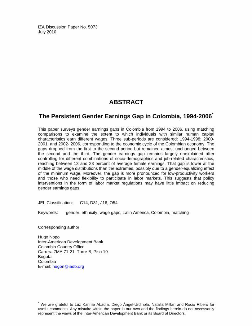
ABSTRACT

The Persistent Gender Earnings Gap in Colombia, 1994-2006* This paper surveys gender earnings gaps in Colombia from 1994 to 2006, using matching comparisons to examine the extent to which individuals with similar human capital characteristics earn different wages. Three sub-periods are considered: 1994-1998; 2000-2001; and 2002- 2006, corresponding to the economic cycle of the Colombian economy. The gaps dropped from the first to the second period but remained almost unchanged between the second and the third. The gender earnings gap remains largely unexplained after controlling for different combinations of socio-demographics and job-related characteristics, reaching between 13 and 23 percent of average female earnings. That gap is lower at the middle of the wage distributions than the extremes, possibly due to a gender-equalizing effect of the minimum wage. Moreover, the gap is more pronounced for low-productivity workers and those who need flexibility to participate in labor markets. This suggests that policy interventions in the form of labor market regulations may have little impact on reducing gender earnings gaps. JEL Classification: C14, D31, J16, O54 Keywords: gender, ethnicity, wage gaps, Latin America, Colombia, matching Corresponding author: Hugo Ñopo Inter-American Development Bank Colombia Country Office Carrera 7MA 71-21, Torre B, Piso 19 Bogota Colombia E-mail: [email protected]

* We are grateful to Luz Karime Abadía, Diego Ángel-Urdinola, Natalia Millan and Rocio Ribero for useful comments. Any mistake within the paper is our own and the findings herein do not necessarily represent the views of the Inter-American Development Bank or its Board of Directors.

3

1. Introduction

From a gender perspective, Colombia has experienced important changes in the labor market

during the last three decades. The increase in the labor market participation rate of Colombian

women has been the highest in a region where the female participation rate has increased

substantially. Elías and Ñopo (2010) report that while in 1980 the participation rate of

Colombian females was the second lowest in the region, only above that of Costa Rica, by 2004

it was the highest in the region, equaled only by Uruguay. Restricting attention to the period

between 1994 and 2006, the increase in female labor force participation in Colombia is the third

highest in the region, only after Venezuela and Peru. Interestingly enough, the female

unemployment rate over the past two decades has steadily been about 5 percentage points higher

than that for men (Sabogal, 2009).

While there still remain some gender differences in labor market outcomes, such as

participation, unemployment rates and, as this paper will explore, wages,1 individual

characteristics also vary considerably across gender. Females have more years of education,

while men tend to have the potential to accumulate more experience in the labor markets. In

addition, there are important differences in the occupational choices of men and women. For

example, most people who report being a household servant are female, while most construction

workers are male.

The fact that there are still sizeable gender gaps in labor market outcomes is surprising

since Colombia is domestically perceived as an “egalitarian” country regarding gender issues.

Legally, there are tools to promote gender equality such as Articles 13 and 43 of the

Constitution, or Article 143 of the Labor Code, which explicitly states that employers should pay

equal wages for equal jobs. In addition, laws have been passed to give more protection to

women—which may have provided disincentives to hire them. For example, Law 50 in 1990

specifies that all female workers in a state of pregnancy have the right to a 12-week paid leave

and that a female worker cannot be fired due to pregnancy. Despite the strong improvement in

the labor market characteristics of women, especially regarding education, and the legal

1 In this paper we interchangeably use the terms “wages” and “earnings” to refer to labor income, either in the form of an employer-employee relationship or in the self-employment and entrepreneurship. More specifically, we will use hourly labor income from the main occupation as the outcome variable of analysis.

4

framework to promote equality, the gender wage gap in Colombia has changed little during the

last 20 years.

One relevant question on that regard is how much of the gender wage gap can be

explained by existing differences in observable characteristics. Traditionally, this question has

been answered using the Blinder-Oaxaca (BO) decomposition, which uses the estimated

differences in Mincerian equations to answer questions such as: “What would the earnings of the

average woman have been if her labor market characteristics were those of the average man?” In

this paper we adopt a non-parametric alternative to the BO decomposition that (i) addresses the

traditional BO question not only for averages but also, and more interestingly, for the distribution

of wages; and (ii) emphasizes the role of the gender differences in the supports of the distribution

of observable human capital characteristics.

The methodology generates synthetic samples of individuals by matching males and

females with the same observable characteristics. By matching individuals in several dimensions,

we compare comparable individuals. The method allows us calculate the earnings distribution of

the sample of females had their observable characteristics resembled those of the sample of

males. Just like alternative decomposition methods, this approach, developed by Ñopo (2008)

allows us to decompose the observed gap into a component due to differences in characteristics

and an unexplained portion. However, in addition, we can also determine how much of the

calculated gap is accounted for by the outcomes of men and women out of the common support.

This issue is often neglected in the gender wage gaps literature and allows for a richer

exploration of gender wage differentials in Colombia.

2. The Literature on Gender in the Colombian Labor Markets Several studies have measured the average gender wage gap in Colombia using Mincerian

equations and decomposing the gap following BO methodology (Tenjo, 1993; and Tenjo, Ribero

and Bernat, 2006). In general their findings coincide in pointing out a substantial gender wage

gap which is mostly explained by differences in the rewards to labor market characteristics,

rather than by differences in the characteristics between men and women.

5

Abadía (2005) tries to determine whether the average gender wage gap in Colombia can

be explained by statistical discrimination.2 The intuition is that if firms do not apply statistical

discrimination, the gender wage gap will not change with experience, whereas if they do, the gap

will depend less on easily observable characteristics (such as gender and education). The author

finds evidence of statistical discrimination against women for private wage earners, but not for

public employees.

Angel-Urdinola and Wodon (2006) document the existence of a long-term trend towards

an increase in the gender wage gap in the years following the issuing of a new labor regulation

giving more protection to women and thereby raising the cost of female employment for firms.

In particular, the authors study the effect of Law 50 of 1990, which, as stated above, ensures that

pregnant female workers cannot be fired and that they have the right to a twelve-week paid

leave, on the gender wage gap between 1982 and 2000. Sabogal (2009) finds that the Colombian

gender wage gap is pro-cyclical among the population aged 25 to 55 years old. She finds

evidence suggesting that three mechanisms contribute to the pro-cyclicality of the gap: i) the

additional worker effect, ii) changes in compositions of the formal and informal worker forces

and iii) changes in sectorial composition.

But the literature in Colombia has already been beyond the analysis confined to averages

and has studied gender wage gaps along the distributions of wages, or along its conditional

distribution. Bernat (2007) explores the distribution of the gender gap using discrimination

curves for 2000, 2003 and 2006. The methodology of this paper calculates incidence, intensity

and inequality of discrimination. The author finds that despite the observed reduction in the

average gender gap starting 2000, there have been no major advances in terms of discrimination:

there is evidence of a glass ceiling (barriers for women to reach the top of the earnings

distribution) for professional women and the percentage of women discriminated against actually

grew throughout the period.

Fernández (2006) using the urban subsamples of the 1997 and 2003 Living Standards

Measurement Survey reports gender differences in wages that are not statistically significant.

However, when measuring the gap along the distribution, there are interesting variations. At the 2 Statistical discrimination is a theory that attempts to explain why minorities are paid lower wages. It arises when rational agents use aggregate group characteristics to evaluate individual characteristics, and this implies that agents belonging to different groups may be treated differently. For example, if firms believe that child-bearing age women are more likely to have babies, and therefore have breaks during their careers, than older women, they would pay child-bearing age women lower wages to account for the higher probability of losing the worker.

6

bottom 3 percent of the distribution, there is a gap favoring men, while between percentiles 4 and

85, the wage gap favors women. At the top of the distribution, she finds evidence of the

existence of a glass ceiling, since there is a gap favoring men that reaches 25 percent of hourly

wages. Using quantile regression analysis she also reports that the gap is mostly due to

differences in rewards rather than observable characteristics.

Badel and Peña (2009) use the Colombian Household Surveys to measure the gender

wage gap for individuals between 25 and 55 years of age in the seven main cities in 1986, 1996

and 2006. The gender wage gap for their sample is always positive, significant, and displays a U-

shape with respect to earnings: women’s wages fall further below men’s at the extremes of the

distribution, whereas they are closer around the middle of the distribution. The authors also

employ quantile regression techniques to examine the degree to which differences in the

distribution of observable characteristics explain the Colombian gender gap. In line with most of

the literature, they find that the gap is largely explained by differences in the rewards to human

capital characteristics. Innovatively, they also account for selection as female participation in

Colombia is far from universal, and thus self-selection of women into work is important. Their

results suggest that selection accounts for roughly 50 percent of the observed gender wage gap.

That is, if all women worked, the observed gender wage gap would be 50 percent higher than

what it is today. The selection effect in Colombia is positive and therefore more able women

self-select into work.

This paper contributes to the previous literature in at least two dimensions. First, we

provide estimations of the gender wage gap between 1992 and 2006, a period that includes

booms and recessions. Second, we also decompose the gaps using an alternative methodology to

BO, with the two methodological advantages outlined above: precision (as it compares

comparable individuals regarding human capital characteristics, providing more precise

measures of the unexplained components of the wage gaps) and information (as it allows us to

explore the unexplained gender wage gaps along the distributions of several variables).

3. Matching and Gender Wage Gap Decompositions In order to disentangle the extent to which gender wage gaps in Colombia can be attributed to

observable differences in characteristics we follow the approach introduced by Ñopo (2008).

This method, as a non-parametric alternative to the traditional Blinder-Oaxaca (BO)

7

decompositions, is based on a matching-on-characteristics approach (characteristics that the

labor markets reward). The algorithm for such matching, in its basic form, can be summarized as

follows:

• Step 1: Select one female (without replacement) from the sample.

• Step 2: Select all males who have the same characteristics as the female

previously selected.

• Step 3: With all the individuals selected in Step 2, construct a synthetic

individual whose wage is equal to the average of all of them and “match” him to

the original female.

• Step 4: Put the observations of both individuals (the synthetic male and the

female) in their respective new samples of matched individuals.

• Repeat steps 1 through 4 until it exhausts the original female sample.

The application of this matching algorithm delivers three sets of individuals: (i) those

females with observable characteristics for which there are no males to do the matching, (ii)

those males who were never selected because there is no female with the same observable

characteristics and (iii) those females and males who were matched. By construction, the set of

matched females and males shows no differences in the distribution of characteristics, so any

differences in wages that could remain in this set cannot be attributed to gender differences in

observable characteristics. They are instead due to unobservable characteristics (discrimination

probably being one of them).

This method emphasizes gender differences in the supports of the distributions of

observable characteristics to develop wage gap decompositions in the spirit of that proposed by

Blinder and Oaxaca. It divides the gender wage gap into four additive elements:

∆=(∆x+∆f+∆m)+∆0 where:

• ∆x is the part explained by males and females having individual characteristics

distributed differently over their common support.

• ∆f is the component of the wage gap that exists because for some

combinations of female characteristics there are no comparable males.

8

• ∆m is the component of the wage gap that exists because some combinations

of characteristics that men have are not reached by women.

• ∆0 is the part that cannot be explained by differences in observable

characteristics.

The first three components can be attributed to the existence of gender differences in

individuals characteristics that the labor market rewards, while the last is due to the existence of

a combination of both unobservable (by the econometrician) differences in characteristics that

the labor market rewards and discrimination. The last component is comparable to the one that is

due to the differences in rewards to observables characteristics in the traditional BO approach,

but restricted to the common support of those characteristics.

The BO decomposition based on linear regressions suffers from a potential problem of

misspecification due to differences in the supports of the empirical distributions of individual

characteristics for females and males (gender differences in the supports). This is due to the fact

that there are combinations of individual characteristics for which it is possible to find males in

the labor force, but not females (for example, males who are in their early thirties, married, and

holding at least a college degree). There are also combinations of characteristics for which it is

possible to find females, but not males (for example, single females who are migrants, in their

late forties, and have less than an elementary school education). With such combinations of

characteristics, one cannot compare outcomes across genders.

By not considering this restriction, the BO decomposition is implicitly based on an “out-

of-support assumption”: it becomes necessary to assume that the linear estimators are also valid

out of the supports of individual characteristics for which they were estimated.

Along with the misspecification problem associated with gender differences in the

supports, the traditional BO approach is only informative about the average unexplained

difference in wages. It is therefore not capable of addressing the distribution of these

unexplained differences. The matching technique enables us to highlight the problem of gender

differences in the supports and also to provide information about the distribution of the

unexplained pay differences, as will be shown in the following sections.

9

4. The Data Data for this paper are drawn from household surveys quarterly collected by the Colombian

National Statistical agency (DANE). Up to the year 2000 the survey included an extensive labor

markets module in its second quarter release every other year, including information on labor

earnings, social security coverage and firm size, among other areas. Since then the extensive

labor module has been included yearly. In this paper we use available data from 1994 to 2006,

that is, for the earlier period we count with biannual and for the later with annual data.3 As a

result we use 10 shifts of the survey for the period under analysis.

Figure 1 below illustrates the evolution of real hourly wages for females and males

during that period along with the evolution of the growth rate of the real GDP per capita. As

shown in the figure, three qualitatively different periods can be identified. The first, from 1994 to

1998, displays real wage growth but with marked fluctuations. A second period, from 2000 to

2001, is characterized by substantial reductions in real wages (the annualized reduction in real

wages was above 10 percent), and a third period from 2002 to 2006 characterized by sustained

growth in real wages. Furthermore, the periods distinguished from the evolution of real wages

coincide with the periods that one would distinguish when analyzing the evolution of GDP

growth in the country. The first period, 1994-1998, is characterized by a slowdown of overall

economic activity, reaching a limit by the end of the period. A steep economic decline can be

seen in 2000 and up to 2001, followed by a sustained growth since 2002.

3 Even though there is earlier information, we decided to begin our analysis in 1994 because of two main reasons. First, during the 1980s the right tail of the income distribution was truncated, and second, there was a major reform to the health system in 1993 (Law 100), with profound impacts on labor markets, particularly in regard to formality and wages (Camacho, Conover and Hoyos, 2009; Santa María, 2009 and Santa María, García and Mujica, 2008).

10

Figure 1. Evolution of Real Hourly Wages 1994 – 2006

Source: Household Surveys 1994 – 2006

It is for these reasons that our analysis of the evolution of wage gaps will be organized

around these three periods. This paper would then provide a recent approximation to the

discussion about the relationship between gender earnings disparities and the economic cycle in

Colombia. As it will be shown, the evidence we provide here is mixed on that regards. There is a

substantial drop in the gender earnings gap from the first to the second period but almost no

change thereof.

In each of the three periods we pool the data sets for the years available during each

period, using the corresponding expansion factors of each survey to maintain its

representativeness. We restrict the analysis to the 10 largest metropolitan areas,4 and in these

cities we focus on working individuals between 18 and 65 years old reporting positive earnings

(that is, we drop unpaid workers from the analysis and those who do not report a wage), working

between 10 an 84 hours per week and with no missing information regarding their observable

characteristics. Also, for each year and gender we drop the top 1 percent of the earnings

distributions as these are likely measurement-error outliers for the variable of interest. Table 1

below reports relative wages by different sets of observable individual characteristics,

4 Barranquilla, Bucaramanga, Bogotá, Manizales, Medellín, Cali, Pasto, Villavicencio, Pereira and Cúcuta.

11

normalizing them such that average females’ wages are set equal to 100 at each period. The

gender wage gap was higher during the earlier period (reaching almost 18 percent of average

females’ wages) and similar between the intermediate and the later period (at almost 14 percent).

12

Table 1. Relative Hourly Wages by Characteristics

Source: Household Surveys 1994-2006

Many interesting features arise. Regarding individuals’ life cycle, some gender

differences are worth noting. On the one hand, males reach their earnings peak when they are

between 45 and 54 years old, and this has been the case for the three periods under analysis. On

the other hand, females’ earnings profile over the life cycle has slightly changed during the last

15 years. For the earlier period their earnings peak was achieved when they were 35 to 44 years

Female Male Female Male Female MaleAll 100.0 118.3 100.0 113.8 100.0 113.5Age18 to 24 76.2 † 79.4 74.1 † 76.3 72.4 72.925 to 34 † 102.2 114.0 102.3 109.6 101.3 109.235 to 44 † 113.1 134.1 108.8 127.1 107.0 126.445 to 54 † 106.3 143.6 112.7 135.7 114.7 131.855 to 65 † 89.9 130.7 91.5 124.6 95.0 129.6EducationNone or Primary Incomplete † 50.4 68.4 48.6 61.8 45.5 56.9Primary Complete or Secondary Incomplete † 66.4 85.7 62.6 78.7 58.4 71.4Secondary Complete or Tertiary Incomplete † 109.6 124.2 103.1 116.3 92.8 107.0Tertiary Complete † 223.5 291.8 244.1 286.3 229.4 277.3Presence of children (<6) in the householdNo † 100.9 120.4 102.6 115.6 101.4 115.5Yes † 97.0 113.3 90.5 108.7 94.3 107.2Marital StatusCohabiting † 81.2 94.7 79.2 90.9 81.5 88.7Married † 124.6 144.6 126.4 142.2 129.7 147.9Widowed, Divorced or Separated † 88.4 113.3 90.8 106.7 91.1 107.9Never Married † 95.0 101.4 97.6 101.9 95.0 98.6Presence of other household member with labor incomeNo † 94.7 113.1 101.0 113.8 103.5 113.2Yes † 101.4 121.2 99.6 113.7 98.8 113.7Type of EmploymentEmployer 157.6 † 192.1 185.6 186.3 177.4 † 202.6Self ‐ Employed † 82.3 105.6 71.8 88.2 74.9 89.8Private Employee † 98.8 106.4 105.4 109.0 107.5 105.9Public Employee 178.8 ‡ 183.9 218.0 216.4 233.2 230.4Domestic Servants † 40.2 54.3 46.9 67.2 45.0 64.6Time workedPart time † 129.5 165.8 112.7 155.9 104.6 147.7Full time † 105.0 126.4 113.3 130.0 115.8 131.4Over time † 67.1 96.3 67.8 87.1 70.2 89.1FormalityNo † 73.4 94.6 67.3 81.3 63.3 77.0Yes † 119.2 139.2 129.3 145.6 130.1 142.6Small fimNo † 121.2 † 131.3 134.1 † 139.9 135.7 * 136.9Yes † 75.4 102.9 69.1 90.0 67.3 88.8Economic SectorPrimary 113.5 † 140.8 93.2 † 115.1 123.5 128.2Secondary † 88.3 103.5 91.2 101.4 90.4 98.6Tertiary † 103.5 125.8 102.4 119.3 102.3 120.5OccupationWhite Collar † 128.4 162.4 134.6 156.8 137.5 159.7Blue Collar † 66.3 89.2 65.4 84.6 62.7 80.5Note: † in the name of the category indicates that the wages differences between males and females are statistically different at the 99% level in the three periods.† Means are statistically different at the 99% level‡ Means are statistically different at the 95% level* Means are statistically different at the 90% level

(2002 ‐ 2006)(Base: Average female wage = 100)(Base: Average female wage = 100) (Base: Average female wage = 100)

(1994 ‐ 1998) (2000 ‐ 2001)

13

old. For the latter two periods, however, the peaks are achieved at later ages (between 45 and 54

years old). This may reflect either a secular trend in females’ staying longer in the labor markets,

maintaining their productive cycles and avoiding early retirement; or an increase in effective

labor market experience for females (or a combination of both).

Regarding education, the patterns of skill premium are not surprising, neither for males

nor for females. Males earn more than females in all education categories for all three periods.

The presence of other income earner in the household does not seem to play an important role in

wage differentials. Individuals living in households with children (younger than 6 years of age)

tend to show lower wages than whose living in households with no children, and that difference

has remained constant over the period of analysis.

In regard to marital status, married people earn more than others. Never-married

individuals earn almost the same as those cohabiting, but individuals cohabiting outside of a

formal marriage persistently receive the lowest wages. It is interesting to note, however, that

gender wage gaps are more pronounced among those cohabiting than among those never

married. The highest wage gaps are found among widowed, divorced or separated individuals.

As expected, employers earn much more than private employees, who in turn earn more

than the self-employed, who in turn earn more than domestic servants. The surprising result,

however, is that public employees are at the top of average earnings by type of employment.

Part-time workers (those who work less than 35 hours per week) earn much more per hour than

those working full time who in turn earn more than those working over-time (more than 48

hours). Informal workers earn less than their formal counterparts,5 and those working in small

firms (five workers or less) earn less than those working in larger firms. Services (business and

social) and construction are among the highest paid economic sectors, especially (and

interestingly) for women. On the other extreme, household and personal services is the lowest

paid sector during the whole period of analysis and for both genders. White-collar workers earn

more than blue-collar workers, as expected.

The results reported in Table 1, however, are merely descriptive statistics; they do not

take into account the simultaneous role of other observable characteristics in the determination of

wages. Table 2 describes the differences in observable characteristics between men and women

for the three periods under study.

5 In this paper, a worker is considered as formal if she/he contributes to health insurance through employment.

14

Table 2. Observable Characteristics: Descriptive Statistics

Source: Household Surveys 1994-2006.

Working men are slightly older than working women. However, both females and males

are staying longer in labor markets. This is reflected in an older labor force, especially for

females, as shown in the statistics over time. While women in Colombia are more educated than

men, the overall labor force’s education also shows an increasing trend as the percentage of

workers with tertiary and secondary education has increased over the three sub-periods.

Female Male Female Male Female MaleReal Wage 2,225 2,632 1,948 2,217 1,998 2,269Age (%)

18 to 24 19.8 18.6 18.4 17.5 17.2 16.6 25 to 34 36.0 33.8 32.2 32.2 30.5 30.6 35 to 44 27.4 25.5 29.3 27.2 29.0 26.7 45 to 54 12.4 14.6 14.8 15.7 17.7 18.0 55 to 65 4.4 7.5 5.2 7.4 5.7 8.2Education (%) None or Primary Incomplete 11.6 12.2 10.4 11.4 8.8 9.5Primary Complete or Secondary Incomplete 38.5 45.9 37.9 41.0 32.6 35.8 Secondary Complete or Tertiary Incomplete 37.7 30.9 38.9 36.3 42.0 40.6 Tertiary Complete 12.2 11.1 12.7 11.2 16.5 14.1 Presence of children in the household (%) 22.7 29.6 21.3 26.6 19.2 23.5 Marital Status (%) Cohabiting 15.2 24.5 18.9 29.3 19.8 29.8 Married 28.5 41.6 25.9 36.7 24.6 34.9 Widowed, Divorced or Separated 20.6 4.6 23.4 6.7 22.3 7.0Never Married 35.6 29.3 31.8 27.4 33.3 28.3 Presence of other member with labor income (%) 79.5 64.5 73.3 62.1 73.5 63.8 Type of Employment (%) Employer 3.3 7.1 2.6 5.6 2.8 5.9Self ‐ Employed 22.0 26.4 27.3 32.6 26.9 30.9 Private Employee 54.8 58.4 49.7 54.6 50.8 57.0 Public Employee 10.5 7.9 8.0 6.8 6.1 5.7Domestic Servants 9.4 0.2 12.4 0.4 13.4 0.5Time worked (%) Part time 16.5 6.9 21.6 10.5 20.6 8.9Full time 59.6 57.2 49.5 45.2 49.9 45.4 Over time 23.9 35.9 29.0 44.2 29.6 45.7 Small fim (%) 46.3 45.8 52.5 52.3 52.2 48.7 Formality (%) 58.1 53.1 52.8 50.4 54.9 55.7 Economic Sector (%)Primary 0.8 1.8 0.9 2.0 0.8 2.1Secondary 23.5 35.0 20.9 30.5 20.4 32.5 Tertiary 75.7 63.2 78.3 67.5 78.8 65.4 Occupation (%) White Collar 54.2 39.8 50.0 40.4 49.8 41.7 Blue Collar 45.8 60.2 50.0 59.6 50.2 58.3 Observations (Unweighted) 33,411 47,595 22,450 27,417 58,181 68,598Observations (Weighted) 5,863,482 7,992,771 4,183,348 4,840,639 11,817,986 12,837,329

(1994 ‐ 1998) (2000 ‐ 2001) (2002 ‐ 2006)

Note: Using a Pearson's chi‐squared statistic to test the distribution between males and females among categories of each of the variables, weconclude that all are statistically different at the 99% level in each of the three periods.

15

Even though children are more often present in the households of working men, the

prevalence of children has decreased over the period of study, and gender differences have

narrowed. In line with previously reported findings by Amador and Bernal (2009), there have

been important changes in patterns of family formation and dissolution in Colombia, similar to

what has happened in the rest of the region. The percentages of cohabiting individuals have

increased, both for males and females (but cohabitation is higher among males). Combining

formal marriage and cohabitation, there are also important gender differences in marital status.

Approximately two out of three working males are married (either formally or informally), while

less than half of working females in Colombia are in a similar situation.

There are more often other members of the household with labor income for women than

for men. The presence of other income earners at home has not changed for males but has

slightly changed for females. The percentage of females who share the breadwinning

responsibilities in their household has dropped almost 5 percentage points during the period of

analysis, reflecting the increase in female household headship that Colombia and the Region has

experienced. Very few workers are employers (and there are around twice as many male

employers as female employers) and the share of self-employment has increased at the expense

of the share of employees. For males, overtime schedules have increased in Colombia such that

at the latter period almost one half of males reported working more than 48 hours per week. For

females, the data show both an increase in overtime and also an increase in part-time schedules

(at the expense of full-time schedules), reflecting the great deal of heterogeneity present in the

labor markets for females.

Around half of workers (both males and females) are formal employees in small firms.

Transportation is a sector that has gained employment among males, and the prevalence of

white-collar workers has slightly decreased among females and increased among males.

We next turn to the central question of this paper: To what extent can observed gender

differences in wages be explained by gender differences in observable characteristics?

5. Results Table 3 shows different wage gap decomposition exercises for the three sub-periods. Each panel

on the table corresponds to a sub-period. Then, in each panel the decomposition exercises are

shown in columns such that each column adds a variable to the matching set available in the

16

previous one. The first column results from matching females and males in the same survey year,

living in the same metropolitan area and within the same age group. The second column

considers the previous matching characteristics and individuals’ education level. The third adds

upon the second by considering presence of children in the household on top of the previous four

characteristics, and so on. The matching variables considered in Table 3 are those considered as

individuals’ socio-demographics, without considering other job-related characteristics for the

time being.

The first panel on Table 3 shows that during 1994-1998 males earned 18.3 percent higher

hourly labor earnings than females (measured as a percentage of average females’ wages).When

controlling for year, city and age group most of the wage gaps remains unexplained, as only a

wage gap of 0.1 percentage points of average females’ wages can be accounted for by these

characteristics. When adding education to the previous set of matching characteristics, the

unexplained wage gap is even slightly higher, reflecting the higher education of the female

population. Not only that, but also the component that exists because males achieve certain

combinations of characteristics that females do not (∆m) reaches a level close to 2 percent (which

remains after the addition of other socio-demographics). The addition of the other socio-

demographic characteristics slightly reduces the unexplained component of the wage gap (∆0)

and (∆m) but at increases (∆f), the component that exists due to unmatchable females.

As mentioned above, the overall gender wage gap is higher during the first sub-period

than in the other two. After controlling for observable individuals’ socio-demographic

characteristics the pattern remains. In fact, most of the gap remains unexplained after matching

the whole set of socio-demographics. The second most important element, but an order of

magnitude smaller, is the one that exist because females fail to achieve certain combinations of

characteristics that males do; these are well-paid segments of the labor markets.

17

Table 3. Gender Wage Gap Decomposition




Year, Metropolitan Area & Age

+ Education + Presence of children in the HH

+ Marital Status

+ Presence of other wage earner

member in the HH

∆ 18.3% 18.3% 18.3% 18.3% 18.3%∆0 18.2% 19.9% 19.4% 17.5% 18.5%∆M 0.0% 1.8% 2.5% 1.6% 0.7%∆F 0.0% ‐0.1% ‐0.4% 0.8% 1.7%∆X 0.1% ‐3.3% ‐3.3% ‐1.6% ‐2.6%

% CS Males 99.8% 97.4% 93.0% 76.5% 57.6%% CS Females 100.0% 99.3% 97.5% 78.4% 68.3%

1994 ‐ 1998



+ Marital Status


member in the HH

∆ 13.8% 13.8% 13.8% 13.8% 13.8%∆0 13.0% 15.4% 15.8% 13.8% 14.5%∆M 0.0% 2.4% 3.8% 5.1% 4.9%∆F 0.0% ‐0.7% ‐1.2% ‐2.3% ‐2.0%∆X 0.7% ‐3.4% ‐4.7% ‐2.7% ‐3.6%


2000 ‐ 2001



+ Marital Status


member in the HH

∆ 13.5% 13.5% 13.5% 13.5% 13.5%∆0 13.9% 17.5% 17.4% 16.1% 15.1%∆M 0.0% 1.1% 1.5% 1.3% 1.4%∆F 0.0% ‐0.3% ‐0.7% ‐1.3% ‐1.9%∆X ‐0.5% ‐4.7% ‐4.7% ‐2.6% ‐1.0%


2002 ‐ 2006

18

Investigating the effect of job-related individuals’ characteristics on top of the socio-

demographics reported in Table 3 is not a simple task. The curse of dimensionality suffered by

non-parametric approaches, including the present matching approach, presents a challenging

task. As the number of matching variables increases, the likelihood of finding matches

diminishes and hence the size of the common supports, as reported in the last two rows of the

tables. For that reason, in order to leave space for the inclusion of job-related characteristics

some socio-demographic ones will not be considered. The table uses the set of socio-

demographic matching variables that includes year, city age and education and adds the job-

related characteristics one-by-one (as opposed to cumulatively as previously done in Table 3).

The second column of the three panels of Table 4 shows the decomposition that arises

from the use of the socio-demographic characteristics; the third column in the three panels of

Table 3 is copied here to facilitate the comparison. The third columns in Table 4 then add a

dummy variable controlling for whether individuals work in small firms or not (as stated above,

a firms is considered small if it has five workers or less). The fourth column replaces the small

firm dummy for a variable indicating the economic sector in which the individual works

(primary, secondary or tertiary). The fifth column replaces occupation by type of employment,

the sixth instead uses formality and the seventh replaces it by time commitment (part-, full- or

overtime). The eight and last column includes all six job-related characteristics on top of the

basic set of socio-demographics.

Table 4. Gender Wage Gap Decomposition: Job-Related Variables


Year, Metropolitan Area, age & education

& Small Firm

& Sector & Occupation& Type of Empl.

& Formality& Time Worked

Year, Metropolitan Area, age, education & Job‐related

∆ 18.3% 18.3% 18.3% 18.3% 18.3% 18.3% 18.3% 18.3%∆0 19.9% 20.3% 19.3% 23.4% 16.0% 20.3% 24.0% 19.9%∆M 1.8% 3.0% 2.9% 1.8% 7.4% 3.1% 4.0% 1.0%∆F ‐0.1% ‐0.7% ‐0.3% ‐0.1% 2.3% ‐0.5% ‐2.6% 2.3%∆X ‐3.3% ‐4.3% ‐3.6% ‐6.9% ‐7.4% ‐4.6% ‐7.1% ‐4.9%

% CS Males 97.4% 92.4% 90.3% 93.2% 83.7% 93.0% 88.9% 29.6%% CS Females 99.3% 97.3% 96.9% 97.3% 84.6% 97.1% 91.1% 38.6%

1994 ‐ 1998

19

Source: Household Surveys 2000–2001.


The patterns are similar to those depicted in Table 3. Most of the gender wage gaps are

left unexplained by these observable characteristics. Furthermore, the unexplained gender gap

after controlling for observable characteristics is frequently greater than the observed one. The

one-by-one inclusion of job-related characteristics increases the magnitude of the component of

the wage gap attributable to the existence of males with characteristics that are not achieved by

females (ΔM). In the most dramatic case (the one obtained after the addition of type of

employment to the socio-demographic characteristics or columns 6) more than one-third of the

wage gap is explained by this lack of common support in favor of males, in all sub-periods under

analysis. Even more, for the two later periods the role of type of employment accounts for

around one-half of the observed gender wage gaps. This is partly due to the overrepresentation of

women as domestic servants.

The component attributable to the existence of males with characteristics that are not

achieved by females (ΔM) plays a prominent role in explaining the gender gap when controlling

for socio-demographic characteristics alone. However, the component due to the existence of


& Small Firm




∆ 13.8% 13.8% 13.8% 13.8% 13.8% 13.8% 13.8% 13.8%∆0 15.4% 15.4% 14.6% 17.7% 12.7% 16.6% 20.4% 20.1%∆M 2.4% 4.1% 3.5% 2.8% 8.8% 3.7% 5.8% ‐5.9%∆F ‐0.7% ‐1.9% ‐1.5% ‐0.7% 0.2% ‐1.4% ‐3.5% 5.3%∆X ‐3.4% ‐3.8% ‐2.8% ‐6.0% ‐8.0% ‐5.1% ‐8.9% ‐5.7%


2000 ‐ 2001


& Small Firm




∆ 13.5% 13.5% 13.5% 13.5% 13.5% 13.5% 13.5% 13.5%∆0 17.5% 18.0% 16.7% 19.9% 14.5% 17.3% 21.2% 17.9%∆M 1.1% 1.6% 1.6% 0.6% 6.8% 1.3% 2.8% ‐7.2%∆F ‐0.3% ‐1.2% ‐0.7% ‐0.4% 1.8% ‐0.5% ‐1.9% 10.5%∆X ‐4.7% ‐4.8% ‐4.0% ‐6.6% ‐9.6% ‐4.5% ‐8.5% ‐7.7%


2002 ‐ 2006

20

females with characteristics that are not achieved for males (∆f) is just as important when

additionally controlling for job-related characteristics. This implies greater gender segmentation

in job-related characteristics, particularly regarding job type and hours worked.

It is interesting to note, however, that the joint addition of all job-related characteristics to

the basic set of socio-demographics delivers a negative ΔM component, paired with a positive ΔF.

This implies that the existence of females’ access barriers to certain job profiles works in

opposite directions at both extremes of the earnings distribution. Those combinations of human

capital characteristic that females fail to achieve (that is, those of the males out of the common

support) are not linked to higher wages than those of matched males, as evidenced in the left

panel of Figure 2.6 On the other hand, those combinations of human capital characteristics that

females show but for which there are no comparable males are linked to lower wages than those

of the other females. This is shown in the right panel of Figure 2. Note there that the distribution

of wages of females out of the common support is at the left of the distribution of wages of

females in the common support.7

Figure 2. Hourly Wage Distributions (2002 – 2006): After Matching on Full Set of Observable Characteristics

Source: Household Surveys 2002 – 2006

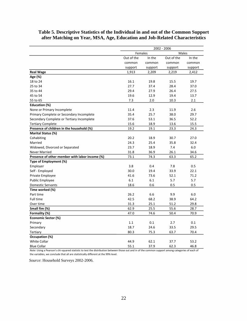
Who are the females and males in and out of the common support of observable

characteristics? The results in Table 5 indicate that males out of the common support differ from

6 Figure 2 is shown here only for the third sub-period. The other two sub-periods, with qualitatively similar results, are available from the authors upon request. 7 Kolmogorov-Smirnov tests for the two differences in distributions shown in Figure 2 deliver rejections of the null hypothesis of equality in both cases.

21

those in the common support in that the former are older, less educated, married, either working

as self-employed or employer, tend to work more overtime in small firms, with less formality,

more in the secondary sector and as blue-collar workers.8 That is, there is no clear pattern

indicating that out-of-support males have better rewarded human capital characteristics than

those in the support. For females, on the other hand, the pattern is similar. Women out of the

common support are older, less educated, more likely to be separated, more likely to be domestic

servants and self-employed than those in the common support. Additionally, women out of the

common support tend to work at both extremes (either part-time or overtime), they work in

smaller firms, with less formality and more as blue-collar workers and in the tertiary sector.

Therefore, unmatched females seem to have combinations of less rewarded human capital

characteristics than those of the females in the common support.

8 As in the case of Figure 2, Table 5 is shown only for the third sub-period. The other two sub-periods, with qualitatively similar results, are available from the authors upon request.

22

Table 5. Descriptive Statistics of the Individual in and out of the Common Support after Matching on Year, MSA, Age, Education and Job-Related Characteristics


Out of the common support

In the common support

Out of the common support

In the common support

Real Wage 1,913 2,209 2,219 2,412Age (%) 18 to 24 16.1 19.8 15.5 19.7 25 to 34 27.7 37.4 28.4 37.0 35 to 44 29.4 27.9 26.4 27.5 45 to 54 19.6 12.9 19.4 13.7 55 to 65 7.3 2.0 10.3 2.1Education (%)None or Primary Incomplete 11.4 2.3 11.9 2.6Primary Complete or Secondary Incomplete 35.4 25.7 38.0 29.7 Secondary Complete or Tertiary Incomplete 37.6 53.1 36.5 52.2 Tertiary Complete 15.6 18.9 13.6 15.5 Presence of children in the household (%) 19.2 19.1 23.3 24.3 Marital Status (%)Cohabiting 20.2 18.9 30.7 27.0 Married 24.3 25.4 35.8 32.4 Widowed, Divorced or Separated 23.7 18.9 7.4 6.0Never Married 31.8 36.9 26.1 34.6 Presence of other member with labor income (%) 73.1 74.3 63.3 65.2 Type of Employment (%)Employer 3.8 0.4 7.8 0.5Self ‐ Employed 30.0 19.4 33.9 22.1 Private Employee 41.6 73.6 52.1 71.2 Public Employee 6.1 6.1 5.7 5.7Domestic Servants 18.6 0.6 0.5 0.5Time worked (%)Part time 26.2 6.6 9.9 6.0Full time 42.5 68.2 38.9 64.2 Over time 31.3 25.1 51.2 29.8 Small fim (%) 62.9 25.5 55.6 28.7 Formality (%) 47.0 74.6 50.4 70.9 Economic Sector (%) Primary 1.1 0.1 2.7 0.1Secondary 18.7 24.6 33.5 29.5 Tertiary 80.3 75.3 63.7 70.4 Occupation (%)White Collar 44.9 62.1 37.7 53.2 Blue Collar 55.1 37.9 62.3 46.8

Males2002 ‐ 2006

Females

Note: Using a Pearson's chi‐squared statistic to test the distribution between those out and in of the common support among categories of each ofthe variables, we conclude that all are statistically different at the 99% level.

23

Having analyzed the role of job-related characteristics in the wage gap decompositions,

we turn back to the basic setup of matching on the full set of socio-demographic characteristics

(year, city, age, education, presence of children in the household, marital status and presence of

other income-earner in the household) and analyze deeper the wage differentials there. Figure 3

shows the gender wage gap decomposition after matching on such set of socio-demographic

variables, year-by-year, illustrating a pattern of diminishing unexplained gender wage gaps for

Colombia during the period of analysis. The component that captures the fact that some males

have combinations of characteristics that are not achieved by females (ΔM) is the second most

important component of the wage gap, but it doesn’t show a decreasing pattern. Consistent with

the results reported in Table 3, this component is higher during the middle sub-period under

analysis.

Figure 3. Gender Wage Gap Decomposition by Year After Matching on the Demographic Set


The reduction in the unexplained component of the wage gap has not been statistically

significant, however, as illustrated in Figure 4. The extremes of the boxes correspond to a 90

percent confidence interval for the unexplained gaps, and the extremes of the whiskers to a 95

percent confidence interval. As reported in the figure, the confidence intervals overlap over time.

Consequently, although there is some evidence that the unexplained gender wage gaps have been

‐10 ‐5 0 5 10 15 20 25

2006 (∆=10.64%)

2005 (∆=13.41%)

2004 (∆=14.37%)

2003 (∆=15.49%)

2002 (∆=14.79%)

2001 (∆=14.12%)

2000 (∆=13.25%)

1998 (∆=19.82%)

1996 (∆=18.36%)

1994 (∆=17.17%)

%

∆0

∆M

∆F

∆X

24

decreasing during the last decade in Colombia, that decrease has not yet been statistically

significant.

Figure 4. Unexplained Wage Gap by Year, Demographic Set


The literature on gender wage gaps for Colombia has already suggested that it is

important to look beyond averages. Badel and Peña (2009) find that the gender wage gap has a U

shape along the earnings distribution. As outlined above, one of the most salient features of the

matching approach to decompose wage gaps is that it not only allows for a computation of the

average decomposition but also for an exploration of its distribution. Our results for the three

sub-periods, shown in Figure 5, are qualitatively similar among them. The unexplained gender

wage gaps are smaller for the middle-income individuals, it is higher at both extremes of the

wage distribution, but slightly more pronounced at the bottom.

What generates the observed U-shape in both the observed and unexplained gender wage

gaps? The minimum wage may be behind the lowers levels of the unexplained gender wage gap

in the middle of the distribution. Because people at the middle of the distribution earn close to

25

the minimum wage,9 it may exert a gender-equalizing effect on intermediate-paying jobs. The

“bite” of the minimum wage varies along the income distribution. It barely affects the wages of

people earning less than the minimum, usually informal workers, is very binding at and around

the level of the minimum wage, and loses importance as one moves along the income

distribution towards high earners (Cunningham, 2007).

When controlling for the demographic set of observable characteristics, the unexplained

gap is slightly higher than when matching on a more basic set, especially at the higher portion of

the wage distribution. When controlling for the full set of socio-demographic and job-related

characteristics the situation is similar: the unexplained gaps above the median of the wage

distributions are higher than before. The novelty arises below the median of the wage

distributions; there the unexplained gaps are substantially smaller than those obtained with the

other sets of matching characteristics. Thus, observable characteristics do a better job of

explaining gender wage differential at the lower portion of the wage distribution.

9 In our sample, approximately 52 percent of males and 58 percent of females earn wages less than or equal to the minimum wage.

26

Figure 5:.Unexplained Gender Wage Gap by Percentiles of the Wage Distribution of Males and Females (1994-2006)

(1994-1998)


(2000-2001)


0

10

20

30

40

50

60

70

80

1 5 9 13 17 21 25 29 33 37 41 45 49 53 57 61 65 69 73 77 81 85 89 93 97

% of fem

ale wage

Wage Percentile

Raw Gap Demographic Set Full Set

0

5

10

15

20

25

30

35

40

45

50

1 5 9 13 17 21 25 29 33 37 41 45 49 53 57 61 65 69 73 77 81 85 89 93 97

% of fem

ale wage

Wage Percentile


27

(2002 – 2006)


The matching approach allows an exploration of wage differentials not only along the

wage distributions but also along the set of observable characteristics. Figure 6 reports

confidence intervals for the unexplained gender wage gaps after matching in the demographic set

along different segments of the labor markets. Most of the cities show similar unexplained

gender wage gaps. The only statistically significant differences in unexplained gaps are found

between Medellin on the one hand, and Bucaramanga and Pereira on the other, being lower in

the former. There is also a pattern for age, as younger people show smaller wage gaps than those

in middle age. The unexplained gaps are highly dispersed among older people (55 to 65 years

old). The unexplained gap along education categories is very similar to that of the whole

distribution; it is higher among those in the low (secondary incomplete) and high education

(complete tertiary) groups, and smaller for those with intermediate education (secondary

complete or tertiary incomplete). The unexplained gaps are also smaller among the widowed,

public employees, full-time workers, those in construction and transportation, white-collar

workers, those in larger firms and formal workers.

0

10

20

30

40

50

60

70

1 5 9 13 17 21 25 29 33 37 41 45 49 53 57 61 65 69 73 77 81 85 89 93 97

% of fem

ale wage

Wage Percentile


28

Figure 6. Gender Wage Gap by Characteristics (2002-2006) Unexplained Gaps after Matching on the Demographic Set

29


6. Concluding Remarks Despite strong improvement in women’s labor market characteristics of women and the

existence of a legal framework to promote equality, the gender wage gap in Colombia has

changed little during the last 20 years. Our results suggest that the gender gap is mostly

unexplained by the existing differences in observable characteristics, both socio-economic and

job-related. Some females seem to be confined to combinations of human capital characteristics

that are less rewarded than those of most of the labor force. The gender wage gap that remains

30

unexplained after accounting for individuals’ and job characteristics displays a U shape with

respect to earnings: it is smaller for middle-income individuals and higher at both extremes of

the wage distribution. This may be due to the gender-equalizing effect of the minimum wage.

Our findings show that the largest unexplained wage gaps are found among less educated

individuals, those who work part-time, in the primary sector/entertainment or household services,

domestic servants, blue-collar workers, informal workers and workers in small firms. These

characteristics, at which the wage gaps are most pronounced, depict two clearly recognizable

profiles within Colombia’s labor markets. One consists of low-productivity individuals, and the

other is comprised of females who, in need of flexibility to participate in the labor markets, have

to work under arrangements of precarious attachment to the markets.

Interesting policy implications in terms of the potential effectiveness—or rather

ineffectiveness—of different measures to decrease the gender wage gaps can be derived from our

results. First, the gender wage gap may be due to discrimination. Some argue that discrimination

will decrease over time on its own as society becomes accustomed to women in the working

force. However, the high participation rates of women in the country, and the fact that the gender

wage gap has changed little in the last decade, suggest that this channel of reduction of

discriminatory practices may not be very effective. This would be especially the case when

considering that “women don’t ask” (Babcock and Laschever, 2003), being less prone to

negotiate and less competitive (Gnezzi, Niederle and Rustichini, 2003; Niederle and Vesterlund,

2007).

Second, as the highest wage gaps are found among low-productivity, vulnerable workers,

who frequently work outside government regulations, it seems that public policy interventions in

Colombia such as standard labor market regulations seem to have little scope to reduce the

gender wage gap. Given the gender imbalance across occupations, particularly the high

proportion of women who work as domestic servants, special regulations geared toward this

group may promise to have some effect on the gender gap (as has been the case with “nanny

laws” in the United States, for example). However, based on the limited success of previous

attempts to enforce the minimum wage and increasing access to health insurance and pension

contributions among domestic servants in Colombia, that promise seems unlikely to be fulfilled.

Third, the gender wage gap may have to do with Colombian women’s dual role as

workers and homemakers, which reduces their labor market attachment and bargaining power at

31

work. Therefore, family-friendly policies, which explicitly take into account the special needs of

female workers, explicitly considering the role of males within households, may have the

potential to reduce the gender wage gap. However, with the information at hand, it is hard to

determine to what extent addressing the gender wage gap depends on the reconciliation of family

and work life. This seems to be a promising field for future research.

32

References Abadía, L.K. 2005. “Discriminación Salarial por Sexo en Colombia: Un Análisis Desde la

Discriminación Estadística.” Documentos de Economía 17. Bogotá, Colombia:

Pontificia Universidad Javeriana.

Albrecht, J., A. Bjorklund and S. Vroman. 2003. “Is There a Glass Ceiling in Sweden?” Journal

of Labor Economics 21: 145-177.

Amador, D. and R. Bernal. 2010 " Marriage vs. Cohabitation: The Effects on Children's Well-

being" Mimeo, Universidad de Los Andes, available at

http://economia.uniandes.edu.co/profesores/planta/Bernal_Raquel/documentos_de_trabaj

o, recovered may 11, 2010.

Amador, D., R. Bernal and X. Peña. In progress. “Trends in Female Labor Participation in

Colombia: Marriage, Children or Education?” Bogota, Colombia: Universidad de los

Andes.

Angel-Urdinola, D., and Q. Wodon. 2006. “The Gender Wage Gap and Poverty in Colombia.”

Labour 20(4): 721-739.

Babcock, L. and S. Laschever. 2003 “Women Don’t Ask: Negotiation and the Gender Divide”.

Princeton, N.J. : Princeton University Press, c2003. xiii, 223 p. ; 24 cm.

Badel, A., and X. Peña. 2009 “Decomposing the Gender Gap with Sample Selection Adjustment:

Evidence from Colombia.” Mimeo, Universidad de Los Andes, available at:

http://ximena.pena.googlepages.com/gender.pdf, recovered May 11, 2010.

Bernat, L. F. (2007) “¿Quiénes son las mujeres discriminadas?: enfoque distributivo de las

diferencias salariales por género” Borradores de Economía y Finanzas No 13, ICESI,

diciembre.

Camacho, A., E. Conover and A. Hoyos. 2009 “Effects of Colombia’s Social Protection System

on Workers’ Choice between Formal and Informal Employment.” Documento CEDE 18.

Bogota, Colombia: Universdidad de los Andes, Centro de Estudios sobre Desarrollo

Económico.

Cunningham, W. 2007. Minimum Wages and Social Policy: Lessons from Developing Countries.

Washington, DC, United States: World Bank Publications.

33

De la Rica, S., J. Dolado and V. Llorens. 2005. “Glass Ceiling or Floors? Gender Wage Gaps by

Education in Spain.” IZA Discussion Paper 1483. Bonn, Germany: Institute for the Study

of Labor/IZA. January.

Elias, J., and H. Ñopo. 2010. “The Increase in Female Labor Force Participation in Latin

America 1990-2004: Decomposing the Changes.” Washington, DC, United States: Inter-

American Development Bank. Mimeographed document.

Fernández, P. 2006. “Determinantes del Diferencial Salarial por Género en Colombia, 1997-

2003.” Desarrollo y Sociedad 58(2): 165-208.

Gneezy, Uri, Muriel Niederle, Aldo Rustichini, “Performance in Competitive Environments:

Gender Differences”, Quarterly Journal of Economics, CXVIII, August 2003, 1049 –

1074.

Niederle, Muriel, and Lise Vesterlund, “Do Women Shy away from Competition? Do Men

Compete too Much?,” Quarterly Journal of Economics, August 2007, Vol. 122, No. 3:

1067-1101.Ñopo, H. 2006. “The Gender Wage Gap in Chile 1992-2003 from a Matching

Comparisons Perspective.” Research Department Working Paper 562. Washington, DC,

United States: Inter-American Development Bank.

----. 2008. “Matching as a Tool to Decompose Wage Gaps.” Review of Economics and Statistics

90(2): 290-299.

Sabogal, A. 2009. “Brecha Salarial por Género y Ciclo Económico en Colombia.” Bogota,

Colombia: Universidad de los Andes. Mimeographed document.

Santa María, M. 2009. “Los Costos No Salariales y el Mercado Laboral: Impacto de la Reforma

a la Salud en Colombia.” Documento de Trabajo 43. Bogota, Colombia: Fedesarrollo.

Santa María, M., F. García and A.V. Mujica. 2008. “El Mercado Laboral y la Reforma a la Salud

en Colombia: Incentivos, Preferencias y Algunas Paradojas.” Bogota, Colobmia:

Fedesarrollo. Mimeographed document.

Tenjo, J. 1993. “1976-1989: Cambios en los Diferenciales Salariales entre Hombres y Mujeres.”

Planeación y Desarrollo 24: 103-116.

Tenjo, J., R. Ribero and L. Bernat. 2006 “Evolución de las Diferencias Salariales de Género en

Seis Países de América Latina.” In: C. Piras, editor. Mujeres y Trabajo en América

Latina. Washington, DC, United States: Inter-American Development Bank.

the persistent gender earnings gap in colombia, …repec.iza.org/dp5073.pdf · the persistent...

Documents