the periods and stability of zz piscium ian clark a senior
TRANSCRIPT

The Periods and Stability of ZZ Piscium
Ian Clark
A senior thesis submitted to the faculty ofBrigham Young University
in partial fulfillment of the requirements for the degree of
Bachelor of Science
Denise Stephens, Advisor
Department of Physics and Astronomy
Brigham Young University
Copyright © 2020 Ian Clark
All Rights Reserved
ABSTRACT
The Periods and Stability of ZZ Piscium
Ian ClarkDepartment of Physics and Astronomy, BYU
Bachelor of Science
In this paper, we present observations of ZZ Psc secured with the 0.4-meter OPO and 0.9-meterWMO telescopes at BYU and augmented with data from the AAVSO to search for previouslyunknown periods for ZZ Psc and verify those that have already been determined. We found whatcould possibly be a previously undiscovered period at 901 seconds. We found that many pulsationmodes change in amplitude over the timescales of about a year. To find stabilities in these periods,we used O-C techniques. We found that nearly all these periods remained constant in observationswith Johnson B, V, and clear filters.
Keywords: Photometry, CCD; Variable Stars (individual), Observing Target: ZZ Psc; PeriodAnalysis; Period Change

ACKNOWLEDGMENTS
I acknowledge my research adviser, Dr. Denise Stephens for guiding me through the process
of producing this work and for helping me become a better scientist. I would like to acknowledge
Dr. Joner and the BYU telescope operators for securing many observations essential to this work.
I also acknowledge Dr. Hintz and Dr. Joner whose knowledge on variable star astronomy helped
move this project forward. I also acknowledge with thanks the variable star observations from the
AAVSO International Database contributed by observers worldwide and used in this research.

Contents
Table of Contents iv
1 Introduction 11.1 Background . . . . . . . . . . . . . . . . . . . . . . . . . . . . . . . . . . . . . . 11.2 The star: ZZ Piscium . . . . . . . . . . . . . . . . . . . . . . . . . . . . . . . . . 2
2 Methods 42.1 Observations and Data Reduction . . . . . . . . . . . . . . . . . . . . . . . . . . . 42.2 Analysis . . . . . . . . . . . . . . . . . . . . . . . . . . . . . . . . . . . . . . . . 5
3 Findings 93.1 Period Identification . . . . . . . . . . . . . . . . . . . . . . . . . . . . . . . . . . 9
3.1.1 Orson Pratt Observatory Data–Clear filter . . . . . . . . . . . . . . . . . . 103.1.2 West Mountain Observatory and AAVSO–V Filter Data . . . . . . . . . . 163.1.3 West Mountain Observatory Data–B Filter . . . . . . . . . . . . . . . . . 24
3.2 Period Decay . . . . . . . . . . . . . . . . . . . . . . . . . . . . . . . . . . . . . 243.2.1 Clear Filter . . . . . . . . . . . . . . . . . . . . . . . . . . . . . . . . . . 293.2.2 V Filter . . . . . . . . . . . . . . . . . . . . . . . . . . . . . . . . . . . . 293.2.3 B Filter . . . . . . . . . . . . . . . . . . . . . . . . . . . . . . . . . . . . 31
4 Conclusion 33
Bibliography 34
iv

Chapter 1
Introduction
1.1 Background
White dwarfs are the end result of most stars that exist, have existed, or ever will exist. These
remnants can be as small as the Earth yet as massive as the Sun. They form when the pressure of a
small to medium mass star can no longer trigger fusion in its now electron degenerate core (usually
made of helium or carbon at this point) and then the outer layers all blow away, leaving the superhot
core–the white dwarf.
These degenerate stellar ashes exist in three main forms (Fontaine & Brassard 2008), and all
have pulsations driven by the κ-mechanism. The grouping of these pulsators is largely based on
what material drives the pulsations. The hottest are the GW Vir stars, also known as DOV stars
(Te f f = 140,000 K), which pulsate by the ionization of carbon and oxygen. The next coolest are
the V777 Her, or DBV stars (Te f f = 25,000 K), whose pulsations are driven by ionized helium.
Lastly, the coolest and by far the most plentiful are the ZZ Ceti, or DAV stars (Te f f = 12,000),
which pulsate by the ionization of hydrogen. This final type is considered to be a natural phase in
the evolution of DA type white dwarfs (Fontaine & Brassard 2008), as the ZZ Ceti grouping lies
1

1.2 The star: ZZ Piscium 2
across the instability strip.
ZZ Ceti stars typically have many pulsation modes, though there is often a single dominant
mode. These pulsations may have stabilities comparable to atomic clocks or even millisecond
pulsars (Mukadam et al. 2001), although others can have pulsation modes that change quickly or
even disappear and reappear with seemingly little warning (Kleinman et al. 1998). The frequency
stability (and pulsation amplitudes) of these ZZ Ceti stars is largely dependent on their temperature,
and thus their age, although mass can play a factor as well. Younger ZZ Ceti stars will have lower
amplitude yet more consistent pulsations and shorter periods and fewer pulsation modes. In contrast,
older ZZ Cetis have high amplitude pulsations with longer, albeit less stable periods and many more
pulsation modes (Kleinman et al. 1998). The purpose of this paper is to report the analysis of the
period stability of ZZ Piscium.
1.2 The star: ZZ Piscium
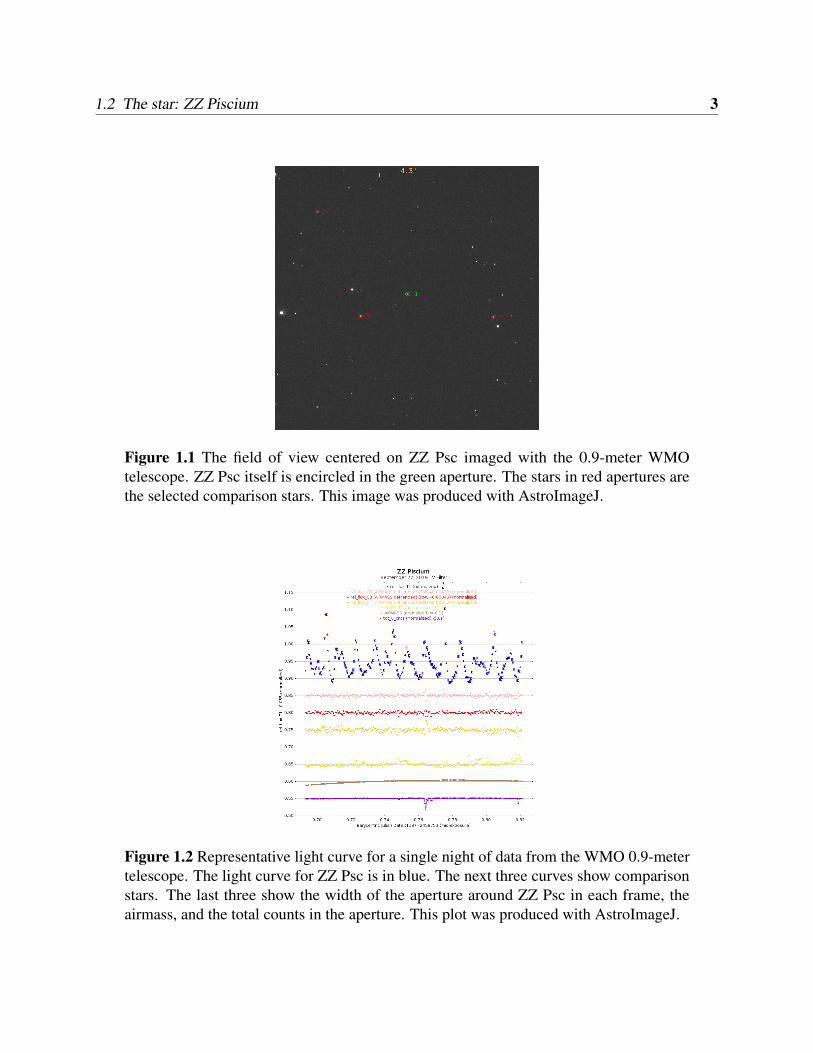
The field of view for the subject of this paper is found in Figure 1.1. We selected this star because
of its bright magnitude, which allowed us to observe it from both observing facilities (see Section
2.1). ZZ Psc is an older ZZ Ceti star as can be noted from its high amplitude pulsations, which can
be seen in the light curves in Figure 1.2. Some other characteristics of this star are, as found in
Romero et al. (2012), Te f f = 11820±200, log(g) = 8.14±0.05, and M/M� = 0.684±0.030.
1.2 The star: ZZ Piscium 3
Figure 1.1 The field of view centered on ZZ Psc imaged with the 0.9-meter WMOtelescope. ZZ Psc itself is encircled in the green aperture. The stars in red apertures arethe selected comparison stars. This image was produced with AstroImageJ.
Figure 1.2 Representative light curve for a single night of data from the WMO 0.9-metertelescope. The light curve for ZZ Psc is in blue. The next three curves show comparisonstars. The last three show the width of the aperture around ZZ Psc in each frame, theairmass, and the total counts in the aperture. This plot was produced with AstroImageJ.
Chapter 2
Methods
2.1 Observations and Data Reduction
We performed the first observations of ZZ Psc at the 0.4-meter Orson Pratt Observatory David
Derrick telescope at Brigham Young University-Provo. We conducted these observations in a clear
filter to ensure acceptable signal to noise ratio. These observations started at 120 seconds, but we
later reduced them to 60 seconds because the SNR was still acceptable and the shorter cadence
would allow for better period detection. Observations at OPO ran from September - November
2018 with some additional observations in August 2019.
We conducted further observations in the V and B filters with the 0.9-meter telescope at BYU’s
West Mountain Observatory. The larger telescope made for the possibility of observing in different
filters and for a much improved signal to noise ratio for this star. Observations ran from September
to October 2019 with this telescope. The exposure times we used at the West Mountain Observatory
for these data were 20 and 30 seconds for the V and B filter data, respectively. To augment the V
filter data, we retrieved archival data from AAVSO (VanMunster, T., 2018, Observations from the
AAVSO International Database, https://www.aavso.org).
4

2.2 Analysis 5
We reduced the data using standard IRAF (Tody 1986) procedures. We produced the light curves
and photometric data with AstroImageJ (Collins et al. 2017).
2.2 Analysis
We extracted the periods for ZZ Psc with both Peranso (Paunzen & Vanmunster 2016) and Period04
(Lenz & Breger 2014). The reason behind this apparent redundancy is the fact that some ZZ Ceti
stars can have pulsation modes that produce both sinusoidal and unusually shaped light curves, and
so we sought a variety of period analysis techniques available to these two programs to extract as
many periods as possible and to determine what algorithms might be best to find the periods of this
star. We used the periods listed in Kleinman et al. (1998), Patterson et al. (1991), and McGraw &
Robinson (1975) to determine a good comparison baseline and also as a cursory look at the potential
variability of the periods of these stars that would be further analyzed (see Section 3.2).
There were a number of period extraction algorithms that we selected for use in Peranso, which
shall be described with their potential advantages and therefore our reasons for using them.
• Lomb-Scargle (Scargle 1982) is described as a Fourier Transform based analysis package
useful for finding weak periodic signals in unequally spaced data. Knowing the often low-
amplitude pulsations of ZZ Ceti stars and long breaks between data sets, this seemed an
excellent analysis package to use for this research.
• CLEANest (Foster 1995) is a Fourier Transform based analysis package similar to Lomb-
Scargle, but it is also effective at finding multiple signals in a data set. As described in Section
1.1, such multiperiodicity is common to ZZ Ceti stars and so using such an analysis package
would potentially find extra periods that otherwise would have been missed.
• ANOVA (Schwarzenberg-Czerny 1996), or ANalysis Of VAriance, is a polynomial based
analysis package. The Peranso manual (Paunzen & Vanmunster 2016) suggests this to be an

2.2 Analysis 6
excellent analysis package to use when one is unsure of which specific analysis package to
use. As it says, its qualities include damping out alias periods and sharply improving peak
detection. ANOVA also allows the user to select the number of harmonics the algorithm will
search for. This may help find additional pulsation modes, but at the same time may introduce
alias periods or lower period detection strength at higher harmonics (see Figure 2.1 for a
comparison between ANOVA periodograms used with four versus two harmonics).
(a) (b)
Figure 2.1 ANOVA periodograms produced by Peranso for ZZ Psc using a) two harmonicsand b) four harmonics. The extra periods found in the 4 harmonic case can be either trueperiods or alias periods based on the rest of the data. Also note the detection strengths.With fewer harmonics, the detections are much stronger. There is therefore a tradeoff–witha higher number of harmonics in the test there is a chance of finding more periods at theexpense of detection strength.
• PDM (Stellingwerf 1978), or Phase Dispersion Minimization, based on what we have read,
sounded like the ideal analysis package for this work. It is one that is best used on sparse
sets of data over a long period of time with non-sinusoidal light curves, like those that can be
produced by some ZZ Ceti type stars.
We also chose to perform analysis with Period04, which uses its own Fourier transform based
calculations to detect periods. We chose to use this software as well since it is a very powerful
program that is a common favorite of variable star observers.

2.2 Analysis 7
After testing these various period analysis programs and packages, we found that Period04,
Lomb-Scargle, and CLEANest tended to give the best results. The Lomb-Scargle and CLEANest
results were nearly identical with only slight variation in period detection strength and so only
results from Lomb-Scargle will be reported out of the two. For the August 2019 data for OPO,
PDM gave much closer periods to what was expected.
The quality of the results is measured by the amplitude of period detection (theta values)
primarily, in the case of the Peranso analysis packages. As for Period04, the amplitude is reported
simply as amplitude. The results’ consistency and agreement with the literature play a factor as
well, albeit a more minor one. This is because, as discussed, the periods of ZZ Cetis are prone to
change and the papers that we used to compare results with are all several years old and several
years apart from each other. Still, we did comparisons with these for the sake of consistency and
good science. The results are given in Tables 2 through 10. To see which periods have been given in
literature so far, see Table 1.

2.2 Analysis 8
Table 1. Periods noted in the literature for ZZ Psc.
Paper Periods (sec)
Kleinman et al. (1998) 110, 117, 237, 284
355, 400, 500, 552
610, 649, 678, 730
771, 809, 860, 894
915, 1147, 1240
Patterson et al. (1991) 186.1, 242.9, 267.9, 614.9
272, 401, 499, 597
1280, 2650
McGraw & Robinson (1975) 209.6, 612.858, 824.674
930.925, 1015.54

Chapter 3
Findings
3.1 Period Identification
We searched for periods in blocks of data to better find any potential changes in period. Because we
do not expect the rate of period change to be too drastic, data sets that are within about two months
of each other went into the same block. Many of the periods we found here were nearly identical to
those that were found in the literature with many others being similar yet still very close, suggesting
that these periods are those that have been previously discovered and therefore are likely to be the
same periods that have changed over the years. We marked these periods as those that we should
look at for potential period changes in Section 3.2.
The 901 second period could possibly be new, since it is fairly distant from any other period (the
closest being 894 found by Kleinman et al. (1998)), yet it still is in the expected range for periods
for ZZ Psc and it has been detected in multiple data sets and/or with multiple algorithms. Oddly
enough, this particular period, whether new or not, seems to disappear and reappear frequently, or at
least change drastically in amplitude as a comparable period is seen in some of the aforementioned
papers but not all and it was only found in a few of the datasets.
9

3.1 Period Identification 10
3.1.1 Orson Pratt Observatory Data–Clear filter
This data set covers a very good span of time, so it is among the best data for analysis, even if it
was done with a smaller telescope. We noticed that there are a handful of periods that are similar to
those that had been discovered by previous studies (see Tables 1, 2, and 3), although there are some
slight variations with many of these periods. These small variations are to be expected because
again, the older, higher amplitude ZZ Ceti stars like ZZ Psc will have their periods change more
quickly than younger, lower amplitude pulsators of the same family. What is intriguing is that many
of these periods are as close as they are to what has been discovered previously, even though the
latest of these studies was done nearly twenty years ago.
Also worthy of note is that the periods are very different between the two data blocks. This is
likely because the August 2019 data block is rather small, so it was more difficult to definitively
detect many periods from this block. Some variation is expected since this data set was taken nearly
a year later and Kleinman et al. (1998) have found that the periods of this star will change on such a
timescale. Even with how different the 2019 data block is compared to the one from 2018, these
data are not to be discounted and there is the possibility that some of these periods are the same as
those found in the September-November 2018 data blocks and they have simply changed. More
discussion on these period changes will be given in Section 3.2.1.
Lastly, there are several periods here that are not similar or even close to what has been
previously discovered (they are at least ten seconds removed from a previously discovered period).
The detection strengths of many of these periods may be strong, but it cannot be conclusively said
that these periods are previously undiscovered periods or new periods without the corroboration of
other data sets. Possibly new periods include the 901.08 second period (agreeing with the AAVSO
V data in Peranso) and the 818 second period (agreeing with the WMO B data in Period04).
3.1 Period Identification 11
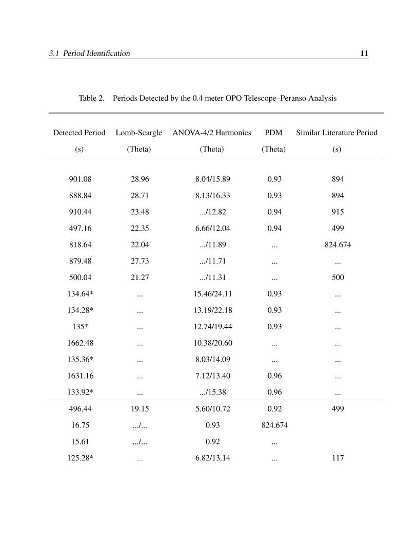
Table 2. Periods Detected by the 0.4 meter OPO Telescope–Peranso Analysis
Detected Period Lomb-Scargle ANOVA-4/2 Harmonics PDM Similar Literature Period
(s) (Theta) (Theta) (Theta) (s)
901.08 28.96 8.04/15.89 0.93 894
888.84 28.71 8.13/16.33 0.93 894
910.44 23.48 .../12.82 0.94 915
497.16 22.35 6.66/12.04 0.94 499
818.64 22.04 .../11.89 ... 824.674
879.48 27.73 .../11.71 ... ...
500.04 21.27 .../11.31 ... 500
134.64* ... 15.46/24.11 0.93 ...
134.28* ... 13.19/22.18 0.93 ...
135* ... 12.74/19.44 0.93 ...
1662.48 ... 10.38/20.60 ... ...
135.36* ... 8.03/14.09 ... ...
1631.16 ... 7.12/13.40 0.96 ...
133.92* ... .../15.38 0.96 ...
496.44 19.15 5.60/10.72 0.92 499
16.75 .../... 0.93 824.674
15.61 .../... 0.92 ...
125.28* ... 6.82/13.14 ... 117

3.1 Period Identification 12
Table 2 (cont’d)
Detected Period Lomb-Scargle ANOVA-4/2 Harmonics PDM Similar Literature Period
(s) (Theta) (Theta) (Theta) (s)
875.88 ... .../... 0.94 ...
888.84 ... .../... 0.94 894
Note. — *We suspect these periods to be artifacts of the cadence of the data. The data above the line
were taken in September-November 2018 and the data below it were taken in August 2019.
3.1 Period Identification 13
(a) (b)
(c) (d)
(e) (f)
(g) (h)
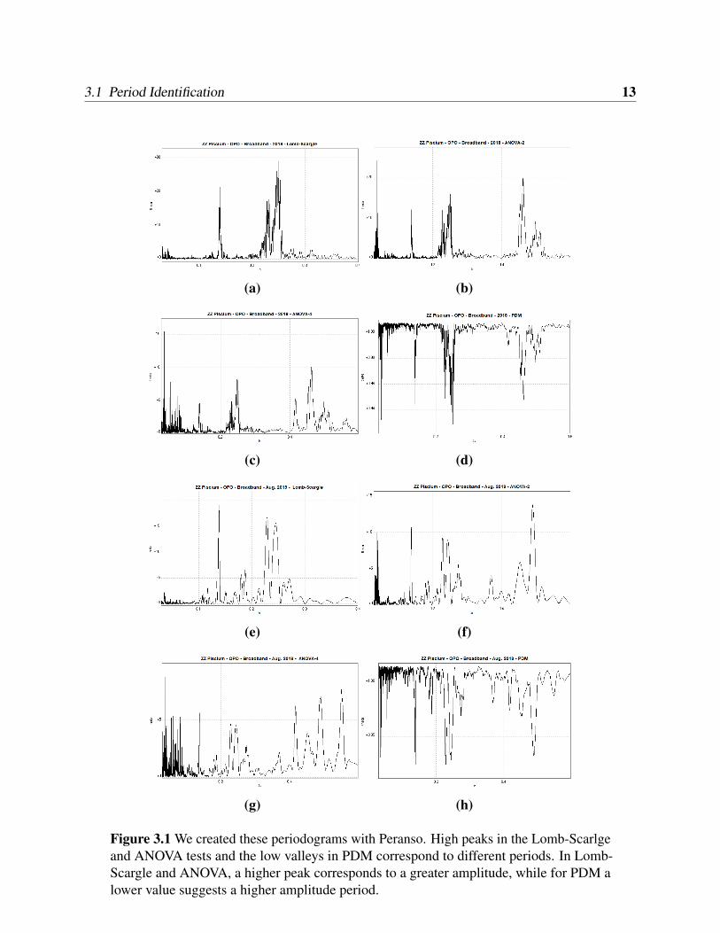
Figure 3.1 We created these periodograms with Peranso. High peaks in the Lomb-Scarlgeand ANOVA tests and the low valleys in PDM correspond to different periods. In Lomb-Scargle and ANOVA, a higher peak corresponds to a greater amplitude, while for PDM alower value suggests a higher amplitude period.
3.1 Period Identification 14
(a) (b)
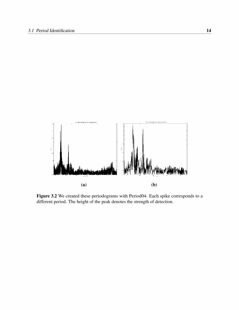
Figure 3.2 We created these periodograms with Period04. Each spike corresponds to adifferent period. The height of the peak denotes the strength of detection.
3.1 Period Identification 15
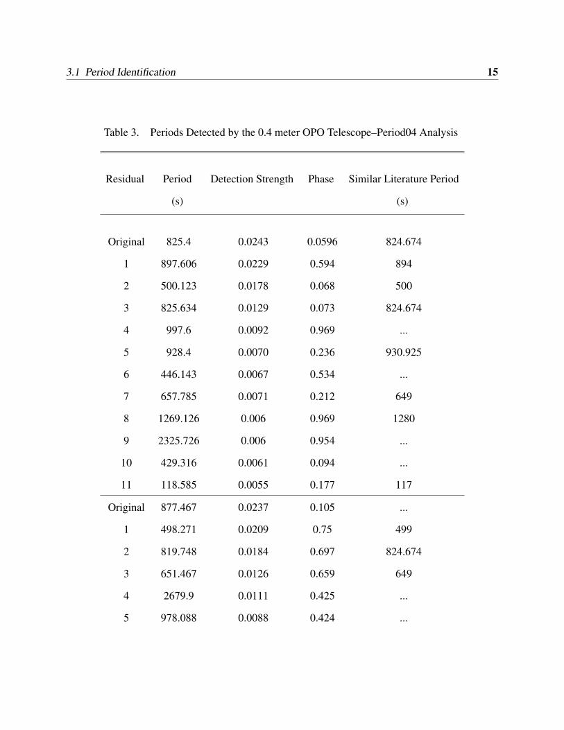
Table 3. Periods Detected by the 0.4 meter OPO Telescope–Period04 Analysis
Residual Period Detection Strength Phase Similar Literature Period
(s) (s)
Original 825.4 0.0243 0.0596 824.674
1 897.606 0.0229 0.594 894
2 500.123 0.0178 0.068 500
3 825.634 0.0129 0.073 824.674
4 997.6 0.0092 0.969 ...
5 928.4 0.0070 0.236 930.925
6 446.143 0.0067 0.534 ...
7 657.785 0.0071 0.212 649
8 1269.126 0.006 0.969 1280
9 2325.726 0.006 0.954 ...
10 429.316 0.0061 0.094 ...
11 118.585 0.0055 0.177 117
Original 877.467 0.0237 0.105 ...
1 498.271 0.0209 0.75 499
2 819.748 0.0184 0.697 824.674
3 651.467 0.0126 0.659 649
4 2679.9 0.0111 0.425 ...
5 978.088 0.0088 0.424 ...

3.1 Period Identification 16
Table 3 (cont’d)
Residual Period Detection Strength Phase Similar Literature Period
(s) (s)
6 676.762 0.0093 0.626 678
7 433.868 0.0085 0.931 ...
8 777.313 0.0078 0.543 771
9 372.571 0.0076 0.841 ...
10 608.71 0.0072 0.872 610
11 911.517 0.0068 0.161 915
Note. — The data above the line were taken in September-November 2018 and
the data below it were taken in August 2019.
3.1.2 West Mountain Observatory and AAVSO–V Filter Data
The data from this filter is unique in that it comes from multiple sources, BYU’s West Mountain
Observatory and the database for the American Association of Variable Star Observers (AAVSO).
We took all care to ensure that the data were compatible and that proper comparison and analysis
could be made. Similar to the clear filter data, the periods found in this analysis largely match those
in the literature, with a few others that are different enough and have significantly high detection
strengths and could therefore be previously undiscovered periods for ZZ Psc, such as the 850 second
period, although further data may be needed to definitively say. The only other data set that has a
period that agrees with this one is in the B filter, which did not come much later after this one and
that period is 853 seconds–similar enough to be the same period within error, but different enough

3.1 Period Identification 17
Table 5. Periods Detected by the 0.9 meter WMO Telescope (September 2019)–Peranso Analysis
in V filter
Detected Period Lomb-Scargle ANOVA-4/2 Harmonics PDM Similar Literature Period
(s) (Theta) (Theta) (Theta) (s)
859.32 172.54 66.49/137.70 0.74 860
850.68 159.68 60.14/120.32 0.76 860
867.96 159.69 55.10/110.27 0.77 860
500.04 91.46 27.10/54.35 0.87 500
497.15 85.07 24.83/49.81 0.88 500
658.80 23.16 6.17/12.15 0.97 649
842.4 124.16 41.9/82.56 0.82 ...
1717.56 ... 36.56/72.20 ... ...
903.96 14.72 4.51/8.83 0.98 894
901.08 10.64 2.74/5.47 0.99 894
that it could be another entirely.
Something interesting to note is that on first glance many of the periods that appear in the WMO
data block seemingly did not appear in the AAVSO data from nearly a year earlier and vice versa
(see Tables 5 and 6 and compare to Tables 7 and 8). This would seem to suggest that these periods
disappeared, but upon closer inspection we found that these same periods were indeed present in
both data sets, although they had different, much lower amplitudes in the WMO data block. This
suggests that the amplitudes of certain pulsation modes can change while the periods remain the
same. More discussion will be addressed toward potential period changes in Section 3.2.2.
3.1 Period Identification 18
(a) (b)
(c) (d)
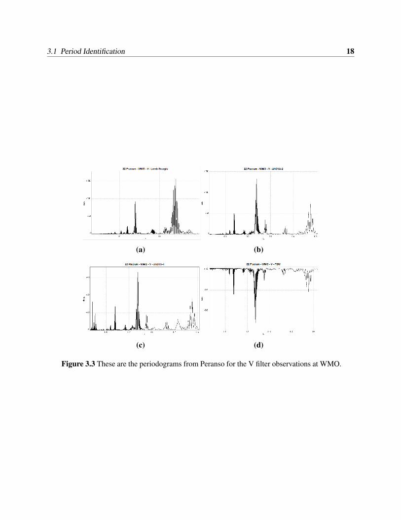
Figure 3.3 These are the periodograms from Peranso for the V filter observations at WMO.

3.1 Period Identification 19
Table 6. Periods Detected by the 0.9 meter WMO Telescope (September 2019)–Period04
Analysis in V
Residual Period Detection Strength Phase Similar Literature Period
(s) (s)
Original 859.66 0.0356 0.8185 860
1 500.191 0.0244 0.9705 500
2 658.01 0.0153 0.9331 649
3 788.9 0.0140 0.4684 ...
4 429.901 0.0118 0.3705 ...
5 954.872 0.0112 0.6843 ...
6 2635.5 0.0104 0.0951 2650
7 371.16 0.0091 0.8304 ...
8 840.544 0.0088 0.1697 ...
9 864.057 0.0076 0.5123 860
10 544.751 0.0070 0.9153 ...
11 317.378 0.0059 0.8276 ...

3.1 Period Identification 20
Table 7. Periods Detected in AAVSO V filter data (July 2018)–Peranso Analysis
Detected Period Lomb-Scargle ANOVA-4/2 Harmonics PDM Similar Literature Period
(s) (Theta) (Theta) (Theta) (s)
842.4 86.91 30.33/59.94 0.82 ...
834.48 84.83 27.89/84.85 0.84 824.674
850.68 83.87 30.01/59.86 0.83 860
901.08 82.84 26.57/52.76 0.84 894
910.44 77.97 24.01/47.84 0.85 915
891.72 77.56 24.58/49.00 0.85 894
859.32 77.09 26.34/52.64 0.85 860
826.56 76.76 23.53/46.94 0.85 824.674
867.96 66.86 21.30/41.64 0.85 860
500.04 40.75 11.15/22.38 0.93 500
502.92 38.31 10.94/20.97 0.93 500
1801.08 ... 33.96/63.89 0.87 ...
1684.08 ... 32.59/58.48 0.89 ...
1652.02 ... 29.50/57.42 0.89 ...
1839.24 ... 26.38/48.03 0.91 ...
1764.36 ... 25.26/49.17 0.91 ...
1717.56 ... 23.25/40.53 0.92 ...
818.64 64.73 18.37/37.53 0.88 809

3.1 Period Identification 21
Figure 3.4 This figure is the Period04 periodogram produced for the V filter data fromWMO.
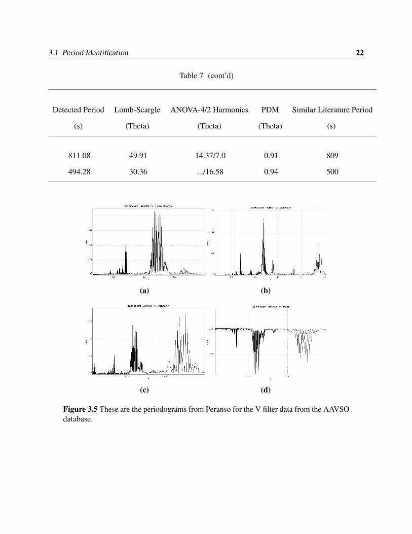
3.1 Period Identification 22
Table 7 (cont’d)
Detected Period Lomb-Scargle ANOVA-4/2 Harmonics PDM Similar Literature Period
(s) (Theta) (Theta) (Theta) (s)
811.08 49.91 14.37/7.0 0.91 809
494.28 30.36 .../16.58 0.94 500
(a) (b)
(c) (d)
Figure 3.5 These are the periodograms from Peranso for the V filter data from the AAVSOdatabase.
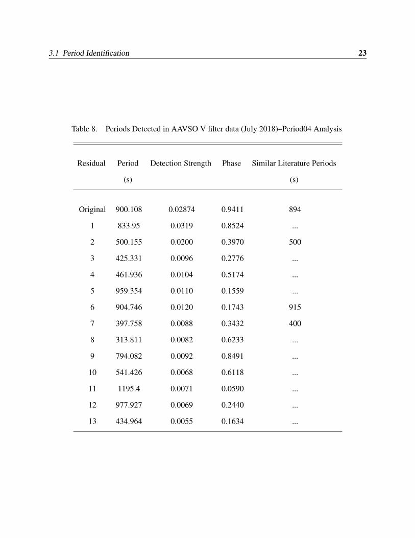
3.1 Period Identification 23
Table 8. Periods Detected in AAVSO V filter data (July 2018)–Period04 Analysis
Residual Period Detection Strength Phase Similar Literature Periods
(s) (s)
Original 900.108 0.02874 0.9411 894
1 833.95 0.0319 0.8524 ...
2 500.155 0.0200 0.3970 500
3 425.331 0.0096 0.2776 ...
4 461.936 0.0104 0.5174 ...
5 959.354 0.0110 0.1559 ...
6 904.746 0.0120 0.1743 915
7 397.758 0.0088 0.3432 400
8 313.811 0.0082 0.6233 ...
9 794.082 0.0092 0.8491 ...
10 541.426 0.0068 0.6118 ...
11 1195.4 0.0071 0.0590 ...
12 977.927 0.0069 0.2440 ...
13 434.964 0.0055 0.1634 ...

3.2 Period Decay 24
Figure 3.6 This figure is the Period04 periodogram produced from the data retrieved fromAAVSO.
3.1.3 West Mountain Observatory Data–B Filter
With less data than on previous filters, the analysis for this data is a bit more speculative. Still, we
found a few periods that are constant between the literature data and what was found in this paper’s
data, including the curiously ubiquitous 500 second period. As for the rest of the periods, it can
be seen in Table 9 that only one period found in the Peranso analysis matches that which has been
found previously. More similar periods were found using Period04, which can be seen in Table 10.
There is a possibility that many of these periods are previously discovered, since many of these
periods are within the expected range and have high detection strengths.
3.2 Period Decay
We analyzed the period decay of ZZ Psc using the procedure enumerated in Axelsen (2014). The
periods we chose to analyze were those similar to the literature as well as periods found in some
data blocks but not others because these periods are those that are most likely to have changed.
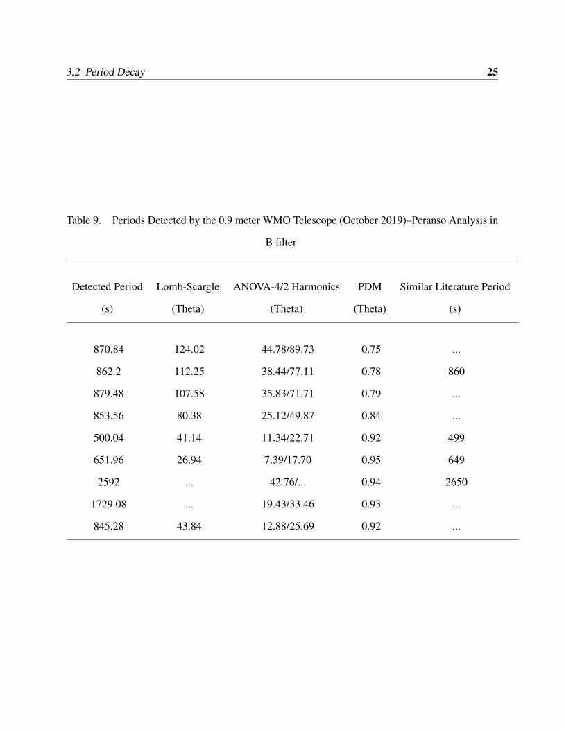
3.2 Period Decay 25
Table 9. Periods Detected by the 0.9 meter WMO Telescope (October 2019)–Peranso Analysis in
B filter
Detected Period Lomb-Scargle ANOVA-4/2 Harmonics PDM Similar Literature Period
(s) (Theta) (Theta) (Theta) (s)
870.84 124.02 44.78/89.73 0.75 ...
862.2 112.25 38.44/77.11 0.78 860
879.48 107.58 35.83/71.71 0.79 ...
853.56 80.38 25.12/49.87 0.84 ...
500.04 41.14 11.34/22.71 0.92 499
651.96 26.94 7.39/17.70 0.95 649
2592 ... 42.76/... 0.94 2650
1729.08 ... 19.43/33.46 0.93 ...
845.28 43.84 12.88/25.69 0.92 ...

3.2 Period Decay 26
(a) (b)
(c) (d)
Figure 3.7 These are the periodograms from Peranso for the B filter data taken at WMO.
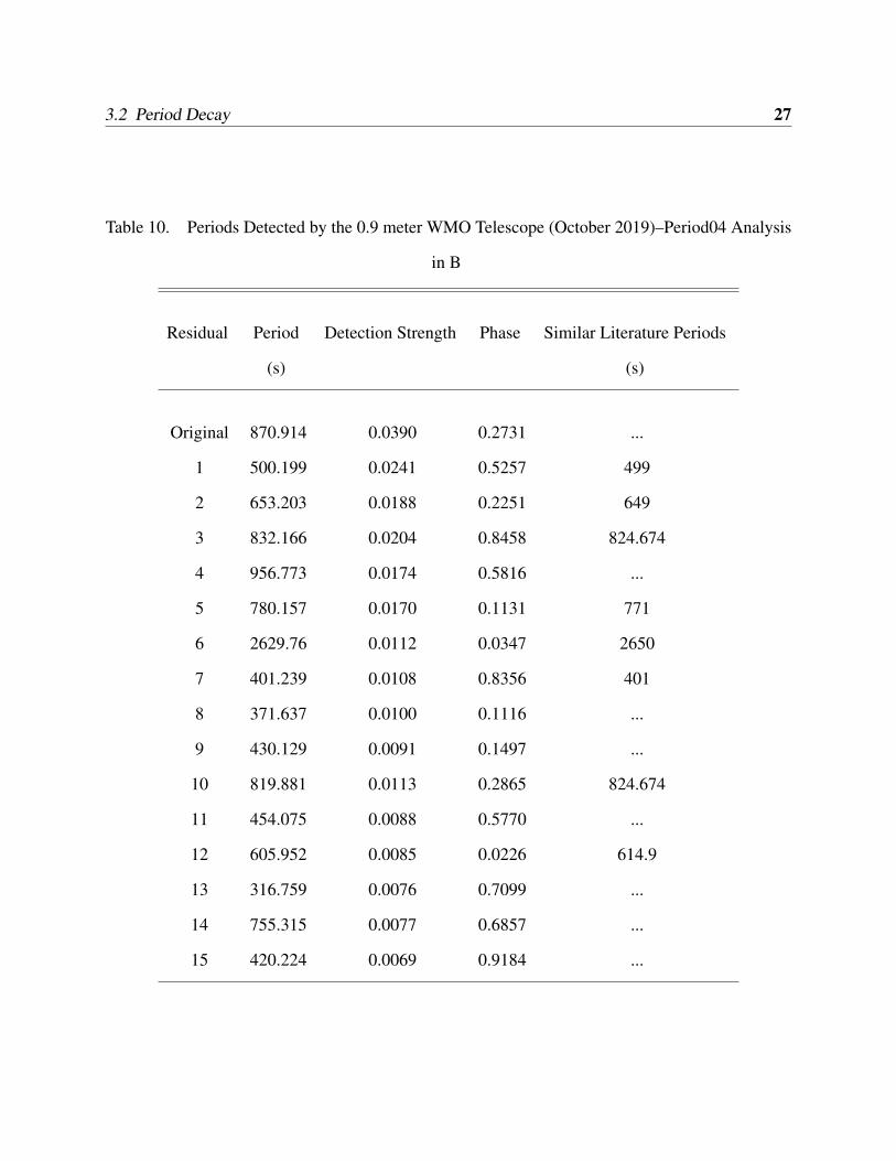
3.2 Period Decay 27
Table 10. Periods Detected by the 0.9 meter WMO Telescope (October 2019)–Period04 Analysis
in B
Residual Period Detection Strength Phase Similar Literature Periods
(s) (s)
Original 870.914 0.0390 0.2731 ...
1 500.199 0.0241 0.5257 499
2 653.203 0.0188 0.2251 649
3 832.166 0.0204 0.8458 824.674
4 956.773 0.0174 0.5816 ...
5 780.157 0.0170 0.1131 771
6 2629.76 0.0112 0.0347 2650
7 401.239 0.0108 0.8356 401
8 371.637 0.0100 0.1116 ...
9 430.129 0.0091 0.1497 ...
10 819.881 0.0113 0.2865 824.674
11 454.075 0.0088 0.5770 ...
12 605.952 0.0085 0.0226 614.9
13 316.759 0.0076 0.7099 ...
14 755.315 0.0077 0.6857 ...
15 420.224 0.0069 0.9184 ...

3.2 Period Decay 28
Figure 3.8 This figure is the Period04 periodogram produced from the data retrieved fromWMO in B filter.
Only the former test was done on the B filter data, since this set only had one block of data. We
gave special attention to the commonly detected 500 second period to get a sense of just how stable
this period is, since it appears in all the data and in two of the papers examined for periods for this
article and has not apparently changed.
As can be seen in Figures 3.9, 3.10, and 3.11, most of the data all hover between +/-0.0008 for
the O-C values, excepting the 2629.76 second period, which is between about +/- 0.015. If the data
were to venture beyond these bounds then we would consider the period’s phase to be changing if,
as stated in Axelsen (2014), the trendline for the data fits a parabolic curve. However, as can be
seen in the figures, such a period change does not apparently occur. We expanded the y-axis limits
to +/-0.05 to get a cleaner look at the data.
According to the above criteria, the periods analyzed (in seconds) are
• For broadband, 825.84, 909, 892.8, 500, 882.72, 897.606 and 877.68
• For V filter, 859.32, 850.68, 867.96, 500.04, 842.4, 901.08, and 826.56

3.2 Period Decay 29
(a) (b) (c)
(d) (e) (f)
Figure 3.9 An assortment of O-C diagrams from ZZ Psc in the broadband filter.
• For B filter, 870.84, 862.2, 879.48, 500.2, 956.773, 2629.76, and 832.166.
3.2.1 Clear Filter
From this data it does not appear any of these periods change, at least not on timescales of about
a year. These periods do indeed appear to change amplitude along such timescales, however, as
evidenced by the fact that different periods showed up as the dominant periods in the different data
sets (see Figures 2 and 3), yet the O-C diagrams do not seem to suggest a frequency change.
3.2.2 V Filter
As is the case with the rest of the data, these periods do not appear to be changing on the timescales
of a year, as can be seen in Figure 3.10.
Another interesting thing to note is that the amplitude for these periods is certainly changing.

3.2 Period Decay 30
(a) (b)
(c) (d) (e)
(f) (g)
Figure 3.10 An assortment of O-C diagrams from ZZ Psc in the V filter.
3.2 Period Decay 31
When searching for periods in the WMO and AAVSO data, it became evident that different periods
showed up in the top periods between the different data sets, but closer analysis revealed that the
same (or at least very similar) periods were present in both datasets, but at different detection
strengths. This was particularly noticeable with the 901.38 second period. It is not reported in Table
6 because Period04 could not detect this particular period.
3.2.3 B Filter
Similar to the other filters, the 500 second period appears stable over the length of the data. In
contrast with the other periods and even with what we see in other periods, the main clusters in the
data set bow up or down on the second day and then back up to more or less the same area on the
third. The 2629.76 and 832.166 periods exhibit this effect most clearly, with the 862.2 and 956.773
second periods possibly showing the same behavior, although on a much more subdued degree.
This behavior can be seen in Figure 3.11.
The unusual thing about this sort of behavior is that it is not something expected. A parabolic
behavior suggests a change in period, yet these parabolas are usually only one half of the curve–they
do not usually curve back. This curve could also be a single phase of a sinusioid, which suggests
the presence of an orbiting body, but we should see behavior like this in other filters if it is an
orbiting body. Also, the work of Kuchner et al. (1998) shows that ZZ Psc is very unlikely to have
any orbiting bodies of significant size.
This bowing is not the only unusual behavior to be found in this filter. The 832.166 second
period is stable for the first two days, but then the clustering falls. This is still not entirely an
unexpected behavior, though. It is possible that the period abruptly changed. Such a thing can
happen, as noted by (Kleinman et al. 1998). However, because this change is so small, it is most
likely the natural shifting of the data that comes as a result of rounding in O-C calculations.

3.2 Period Decay 32
(a) (b)
(c) (d) (e)
(f) (g)
Figure 3.11 An assortment of O-C diagrams from ZZ Psc in the B filter.
Chapter 4
Conclusion
Overall, many of the periods we found were similar to those in the literature, with some slight
differences. When we found a period that was similar but not identical to a previously discovered
one, we knew such a period was a prime candidate to check for period change. We also found a 901
second period that appeared different enough from those in the literature to possibly be a previously
undiscovered period.
All of the periods that we found in V and broadband filters did not appear to change on the
timescale of a year. Additional data will be needed to determine if these periods truly are changing
and how, although it does seem plausible that they are changing, due to the fact that the periods we
found were only slightly different from many of those found in the literature. We can conclusively
say that the amplitudes of these periods change, since their orders of detection between data sets in
the V filter suggest they changed in amplitude relative to each other.
33
Bibliography
Axelsen, R. A. 2014, Journal of the American Association of Variable Star Observers (JAAVSO),
42, 451
Collins, K. A., Kielkopf, J. F., Stassun, K. G., & Hessman, F. V. 2017, AJ, 153, 77
Fontaine, G., & Brassard, P. 2008, PASP, 120, 1043
Foster, G. 1995, AJ, 109, 1889
Kleinman, S. J., et al. 1998, ApJ, 495, 424
Kuchner, M. J., Koresko, C. D., & Brown, M. E. 1998, ApJ, 508, L81
Lenz, P., & Breger, M. 2014, Period04: Statistical analysis of large astronomical time series
McGraw, J. T., & Robinson, E. L. 1975, ApJ, 200, L89
Mukadam, A., Kepler, S. O., & Winget, D. E. 2001, Astronomical Society of the Pacific Conference
Series, Vol. 245, The Most Stable Optical Clocks Known, ed. T. von Hippel, C. Simpson, &
N. Manset, 65
Patterson, J., Zuckerman, B., Becklin, E. E., Tholen, D. J., & Hawarden, T. 1991, ApJ, 374, 330
Paunzen, E., & Vanmunster, T. 2016, Astronomische Nachrichten, 337, 239
34

BIBLIOGRAPHY 35
Romero, A. D., Córsico, A. H., Althaus, L. G., Kepler, S. O., Castanheira, B. G., & Miller Bertolami,
M. M. 2012, MNRAS, 420, 1462
Scargle, J. D. 1982, ApJ, 263, 835
Schwarzenberg-Czerny, A. 1996, ApJ, 460, L107
Stellingwerf, R. F. 1978, ApJ, 224, 953
Tody, D. 1986, Society of Photo-Optical Instrumentation Engineers (SPIE) Conference Series, Vol.
627, The IRAF Data Reduction and Analysis System, ed. D. L. Crawford, 733