We would like to thank the reviewer for her/his encouraging comments regarding the quality of the

submitted work and suggestions. We respond to the specific comments below, where the reviewers’

comments are marked in blue, our responses are shown in black, and the modification in the

manuscript is shown in red.

The paper titled ‘Long term MAX-DOAS measurements of NO2, HCHO and aerosols and evaluation

of corresponding satellite data products over Mohali in the Indo-Gangetic plain’ reports long term

MAX-DOAS observations of AOD, NO2 and HCHO from Mohali, a suburban site in the Indo-

Gangetic plain covering the period of January 2013 – June 2017. The MAPA algorithm is used to

retrieve vertical profile and vertical column densities (VCD) and the results are discussed in detail.

Seasonal and annual trends along with diurnal variation of vertical profiles are discussed and inter-

comparison of the MAX-DOAS measured AOD, NO2 and HCHO with satellite observations are

reported. Finally, they have compared surface volume mixing ratios of NO2 and HCHO with in situ

observations. Whilst the study is strong on analysis, with the methodology explained in detail, the

paper is weak on new results. At present, the manuscript as it stands is more appropriate for a methods

journal, for example Atmospheric Measurement Techniques. No novel results are presented in terms

of improving our understanding of the chemistry or physics of the region, or of the two chemical

compounds and their impacts.

We thank the reviewer for her/his assessment and suggestion. With respect to the suggestion to submit

the paper to another journal, we are sorry if the novelty of the results and the new findings got diluted

by the emphasis on the technical description pertaining to methodology. To address this concern of

the reviewer and strengthen the results of the paper, we have now shifted several technical aspects to

the appendix and improved the discussion of the novel results (for details, see below). We would like

to add that like many other esteemed papers published in ACP, our paper contains methodological

aspects (which are important for a thorough understanding, especially as such studies are lacking from

the region) and also many results with relevance for atmospheric chemistry and physical processes.

In our opinion, the most important novel aspects of our study are the following:

a) In addition to the first MAX-DOAS measurements of NO2 and HCHO vertical column

densities from this under-represented yet crucial part of the world, we report in particular the

vertical profiles of aerosol, NO2 and HCHO for the first time from the Indo Gangetic plain

(and India). This is important information for several aspects of atmospheric chemistry and

physics including atmospheric modelling, satellite retrieval and understanding atmospheric

dynamics. The application of vertical profile includes calculation of airmass factors required

for conversion of slant column densities (SCD) to vertical column densities (VCD),

understanding the atmospheric chemistry at higher altitudes, understanding atmospheric

dynamics, medium and long-range transport, evaluation of the vertical distribution of

chemical tracers in atmospheric models.

A major fraction of the NO2 column was found to be located in the bottom-most layer

extending from surface until 200 meters in all the seasons. We show that during summer and

monsoon seasons, there is a significant fraction of formaldehyde present at intermediate

layers (between 200 and 600m altitudes) and sometimes even higher than the surface

indicating an active photochemistry at these layers. Following the reviewer’s feedback, we

now also discuss the vertical distributions with respect to the ERA5 boundary layer height

(BLH) and found that the seasonal trends in the derived vertical distributions are not strongly

influenced by the BLH. Monsoon season is particularly interesting as the pollutants from the

surface are lifted up to higher altitudes due to deep convection even though the ERA5 BLH

are shallow. NOx and VOCs transported to high altitudes can be transported to a larger area

and can also participate in secondary chemistry producing reservoir species such as PAN.

b) We analyse the annual, seasonal and diurnal profiles of AOD, NO2 and HCHO. We

acknowledge that several AOD measurements and in situ measurements of NO2 have been

reported from this region. However, HCHO (which is primarily a secondary photo-oxidation

product and serves as an indicator of photochemical activity and VOCs) has rarely been

reported. By performing analyses of seasonal and diurnal trends of AOD, NO2 and HCHO,

we identify sources and chemical processes that drive their ambient levels. The sources of

HCHO are indentified to be quite contrasting from majorly photochemical from biogenic and

anthropogenic sources in summer, monsoon and early post monsoon to primary

anthropogenic in winter and late post monsoon. We show that even though the region around

the measurement location has undergone urbanisation, an obvious trend was not observed in

AOD, NO2 and HCHO for more than four years of measurements.

c) Using the measured HCHO and NO2 VCDs, we show that ozone production is sensitive to

NOx and VOCs in winter, but shifts towards NOx in summer. This analysis was originally

performed for the peak daytime hours, which overlaps with OMI overpass and generally

when the maximum in the diurnal profiles of ozone is observed. Following the reviewer’s

suggestion, we have extended this analysis for the morning and late afternoon hours, which

strengthens the observation part of the manuscript.

The main conclusions of the paper are twofold – presenting an inter-comparison with satellite

products, which is a methodology based conclusion and second that ozone production is sensitive to

NOx and VOCs in winter, but more to NOx during the other seasons – not a novel result considering

the past publications globally and in this region. Even the methods section is not new considering it

has been developed in the past by some of the co-authors and has already been used in different parts

of the world.

Hence, I would reject the current paper and encourage submission in a methods journal or ask the

authors to focus more on the observations rather than the observation methodology to decipher novel

results. At present the manuscript, although replete with instrument and retrieval details, does not

include significant results on atmospheric chemistry.

a) We understand the reviewers’ concern that intercomparison with satellite observation is

primarily method based. In our view, putting the technical rigour for the measurements and

intercomparison, which are first of its kind from this region is, however, crucial for the

manuscript. Keeping in view that several studies, especially over India, use only satellite

observations to draw important conclusions regarding NOx and VOC emissions, ozone

production control, VOC source identification, long term trend analyses (e.g. Ghude, et al.

2008, Surl, et al. 2018, Chaliyakunnel, et al. 2019, Hilboll, A., et al. 2013), the evaluation of

various satellite data products is crucial for improving the understanding of atmospheric

chemistry and physics over the IGP. This has not so far been done for the IGP (lines 76 -92 of

the original manuscript). Our study provides the first evaluation of three OMI NO2 data

products and two OMI HCHO data products over the IGP.

b) Quantitative evaluation of the sensitivity of ozone production in different seasons over India

for a period longer than one year has been reported by Mahajan et.al., 2013 using

SCIAMACHY observations for the mean of the years 2002-2013, and by Kumar et al. 2010

and Sharma et al. 2016 using WRF model for the year 2008 and 2010, respectively.

Recognising the rapid urbanisation and industrialisation in the IGP, the sensitivity might

change, and our observations provide a crucial update for the same. Moreover, the unique

feature of our study is that we calculate the sensitivity using ground-based observations as

opposed to the previous studies using SCHIMACY observation (coarse resolution, limited

sensitivity close to the ground) and model simulations (which rely on coarse resolution and

uncertain emission inventories in the region).

In order to focus more on the observations and their interpretation, we have addressed the specific

comments of both the reviewers and restructured the manuscript in the following way:

1. We have made section 2.5 more concise and moved technical details about the various

satellite data products in the appendix.

2. We have modified Figure 6 to also include boundary layer height from ERA5 and included its

discussion with respect to characteristic profiles heights and vertical distribution of aerosol in

section 3.2.

3. We have included a comparison of MAX-DOAS surface VMRs of NO2 and HCHO to

available previous works from India.

4. We have included the HCHO/NO2 ratio for the morning and late afternoon hours in Figure 11

and the relevant discussion in section 3.6.

5. We have restructured section 3.7 to focus more on the interpretation of the retrieved surface

concentrations of HCHO and NO2 and moved technical details about the intercomparison

with in situ observations to the appendix. We have also shown the seasonal variation of the

surface VMR of NO2 and HCHO in the insets of Figures 12 and 13.

6. We have modified the abstract to focus more on the novel findings.

Specific comments:

Measurement technique:

1. Why did the detector temperature have to be adjusted for different seasons? If the temperature was

not stabilised for different seasons, would the diurnal temperature change not lead to the same issue?

Was the DC and offset measured for different temperatures and removed from the spectra according

to the ambient temperature? (line 151-152)

The detector temperature was stabilised using a Peltier cooler and set to values such that the

following two conditions (lines 149-151 of the original manuscript) are met:

1. The detector temperature is lower than the ambient temperature.

2. The difference between the ambient temperature and detector temperature is not more than 20

⁰C.

The complete mini-MAX DOAS instrument was installed in the open, and we had to consider large

variation in ambient temperature to ensure a manageable workload on the Peltier cooler. The ambient

temperature in Mohali ranges from less than 5 °C in winter to up to higher than 40 °C in summer, but

the amplitude of diurnal temperature variation is typically less than 20 °C. Hence, we did not need to

adjust the detector temperature to account for the diurnal temperature change. The dark current

and offset measured for the different temperatures were removed from the spectra according to the

respective detector set temperatures. This information was provided in the original manuscript in lines

151-155. However, to make it clearer for the readers, we have changed to the following in the revised

manuscript (lines 157-158):

“The dark current and offset spectra were recorded every night, and while performing the spectral

analysis, these were subtracted from measured spectra recorded at similar detector temperature.”

2. ‘During the period of measurement, the horizon in the viewing direction was determined by a

residential building with a height of about 40m at a distance of 3 km.’ - This part is not clear. Does it

mean the line of sight has an obstacle within 3 km? Is this why a 1 degree elevation angle was not

used? (line 164-165)

One of the crucial steps for setting up a MAX-DOAS measurement is the elevation calibration. We

performed the elevation calibration using the horizon scan method as described by Donner et.al.,

2020. One of the pre-requisites of this method is the knowledge of the approximate horizon. Several

residential buildings of the city of Mohali and Chandigarh lie in the viewing direction of the MAX-

DOAS instrument, and hence the first estimate of the horizon was calculated using a tall building in

the field of view. The MAX-DOAS instrument is installed at an altitude of 20 m above ground level.

Hence, a 40m high building at 3 km distance would correspond to an angle of 0.38°.

We realise that by mistake, in the manuscript, we write the angle of the visible horizon to be about

0.2°. We apologise for it and correct it in the revised manuscript in line 168. Please note that, even

after this correction, the visible horizon and that determined from using the horizon scan are close to

each other, and further correction is not required.

The reviewer is right that this is also the reason why the measurements at 1° elevation angle were not

used. As can be seen from Fig. F3, the field of view (FOV) of the instrument is rather large, and

typically the RMS of the spectral analysis for the measurements at 1° elevation is substantially larger

than those for the higher elevation angles. This indicates that these measurements are still affected by

the reflected light from the surface. Therefore, we excluded measurements at 1° elevation angle from

further processing.

We have modified lines 145-146 of the original manuscript and added lines 170-172 in the revised

manuscript to include this information:

“The scattered sunlight spectra were recorded for elevation viewing angles 1⁰, 2⁰, 4⁰, 6⁰, 8⁰, 10⁰, 15⁰,

30⁰ and 90⁰ at a total integration time (number of scans × acquisition time for one scan) of 60 seconds

each.”

“We also see from Fig. F3 that the field of view (FOV) of the instrument is rather large (> 0.7°), and

typically the RMS of the spectral analysis for the measurements at 1° elevation is substantially larger

than those for the higher elevation angles. Hence, we excluded the measurements at 1° elevation angle

from further analyses.”

3. What was the calibration process for the instrument? Did the authors perform any spectral

calibration?

The spectral calibration is performed with respect to a high resolved Fraunhofer spectrum. This

information is provided in lines 157-160 of the original manuscript.

“Wavelength to pixel calibrations were performed in QDOAS software

(http://uvvis.aeronomie.be/software/QDOAS/: last access 05.03.2020) (Danckaert et al., 2012) every

time the detector temperature was changed, by matching the structures in a measured spectrum in the

zenith direction at around noontime with those in a highly resolved solar spectrum”

4. ‘Based on the measured radiances at 360 nm, colour index (ratio of measured radiances at 330 and

390 nm) and measured O4 airmass factors (O4 SCD/ O4 VCD), we can classify the sky conditions

into the following seven categories:’ The difference between the upper and lower wavelengths for the

classification is small. Why have the authors have not used radiances from ends of the measured

window? (Line 204-205)

In principle, a wavelength pair with a larger difference between the lower and upper wavelength could

be used for the cloud classification (e.g. 320 nm/440nm) which is close to the ends of the measured

window. However, the chosen wavelength pair has two advantages (Wagner et. al., 2016):

1. The absorption effect of atmospheric ozone is smaller at a longer wavelength, and hence a

longer wavelength (e.g. 330 nm) is more robust to variability in ozone.

2. The variability of the surface reflectance is smaller for shorter wavelength (e.g. 390 nm) as

compared to longer wavelengths (e.g. 440 nm). Hence a global threshold is more robust for

330nm /390 nm wavelength pair.

3. The signal to noise ratio of the measured spectra is rather high, while the changes of the CI

caused by clouds and aerosols are rather strong. Thus, the limitation of the spectral range is

not critical.

5. The sky conditions defined by colour indexes (CI) were not supported by any other supporting

information. Were there any other methods like visual inspection, or comparison with sky images

done for validation? Without validation how can the CI be used for cloud classification – especially

since it is based only on radiances? What were the thresholds used for the classification – what

determines a cloud hole as compared to broken clouds? Although the authors have cited some past

work, that is from different parts of the world, with very different aerosol loading and SZAs – this

information is missing from appendix B. (Line 206-207)

Comprehensive validation of the cloud classification scheme was performed in earlier studies

(Wagner et al., 2014, 2016; Wang et al., 2015). In these publications, the detailed description for the

calibration of the thresholds of the CI and their dependencies on elevation angles and time are also

given, which are applied in this study.

We think that the detail of the method need not be repeated in our study, because they are well

documented in Wagner et. al., (2016). But we added some more information about the general idea of

the algorithm (see below).

The cloud classification scheme is based on the measured radiances at 360 nm, colour index (ratio of

measured radiances at 330 and 390 nm) and the measured O4 airmass factors (O4 SCD/ O4 VCD) (for

details see Wagner et al. (2016)). Besides the absolute values of these quantities, also their temporal

variation and their elevation dependencies are considered. For the analyses presented in this

manuscript, identification of thick clouds and fog was most important, as we retain DOAS

measurements corresponding to sky condition without thick clouds and fog. The identification of

thick clouds and fog are performed according to measured radiance and O4 AMF, respectively. The

thresholds for normalised measured radiances are calculated specifically for our site (Appendix B).

The thresholds for the spread of O4, normalised CI, the spread of the CI and the temporal variation of

the CI are calculated using SZA dependent polynomials provided in Wagner et al. (2016) (Table 1).

We agree with the reviewer that absolute values of the radiances and CI would vary for different parts

of the world depending on several factors which include aerosol conditions and spectrometer

characteristics. In order to account for the spectrometer characteristics, calibration of CI is performed

to get a proportionality constant 𝛽, which relates measured CI (𝐶𝐼𝑚𝑒𝑎𝑠) to the calculated CI (𝐶𝐼𝑐𝑎𝑙).

𝐶𝐼𝑐𝑎𝑙 = 𝛽. 𝐶𝐼𝑚𝑒𝑎𝑠

Only after taking β into account, measured CI is compared to the threshold for cloud classification.

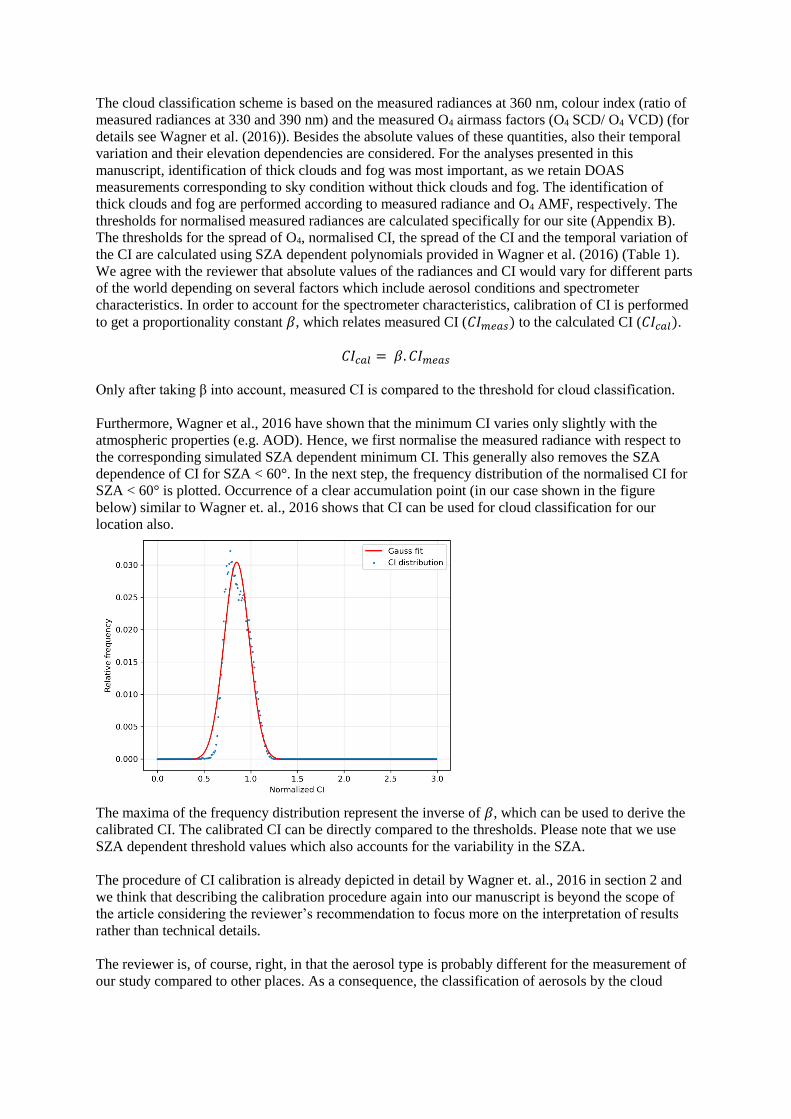
Furthermore, Wagner et al., 2016 have shown that the minimum CI varies only slightly with the

atmospheric properties (e.g. AOD). Hence, we first normalise the measured radiance with respect to

the corresponding simulated SZA dependent minimum CI. This generally also removes the SZA

dependence of CI for SZA < 60°. In the next step, the frequency distribution of the normalised CI for

SZA < 60° is plotted. Occurrence of a clear accumulation point (in our case shown in the figure

below) similar to Wagner et. al., 2016 shows that CI can be used for cloud classification for our

location also.

The maxima of the frequency distribution represent the inverse of 𝛽, which can be used to derive the

calibrated CI. The calibrated CI can be directly compared to the thresholds. Please note that we use

SZA dependent threshold values which also accounts for the variability in the SZA.

The procedure of CI calibration is already depicted in detail by Wagner et. al., 2016 in section 2 and

we think that describing the calibration procedure again into our manuscript is beyond the scope of

the article considering the reviewer’s recommendation to focus more on the interpretation of results

rather than technical details.

The reviewer is, of course, right, in that the aerosol type is probably different for the measurement of

our study compared to other places. As a consequence, the classification of aerosols by the cloud

classification might be slightly different compared to other places. But this is not critical here, because

the main aim – the cloud classification – is hardly affected by these differences.

Following the reviewer’s concerns, we modify lines 211-213 of the original manuscript to provide

further details about the cloud classification and add lines 228-230 in the revised manuscript to

mention the effect of aerosol properties:

“The cloud classification scheme is based on the measured radiances at 360 nm, colour index (ratio of

measured radiances at 330 and 390 nm) and the measured O4 airmass factors (O4 SCD/ O4 VCD) (for

details see Wagner et al. (2016)). Besides the absolute values of these quantities, also their temporal

variation and their elevation dependencies are considered. The thresholds for these quantities (the

spread of O4, the normalised CI, the spread of the CI and the temporal variation of the CI) are

parametrized as polynomials of the SZA as provided in Wagner et al. (2016).” “While the classification of aerosols might be slightly affected by the specific properties of the local

aerosol, the cloud classification is robust to the variability of aerosol properties. However, this is not

critical here, because the main aim – the cloud classification – is hardly affected by these specific

aerosol properties.”

Broken clouds refer to few cloudy patches in the clear sky, while cloud holes refer to clear sky

between clouds. Both cloud holes and broken clouds are detected by a rapid temporal variation of the

observed for normalised CI. In the cloud classification algorithm, the normalised measured CI is

smaller than the threshold CI for broken clouds, and the inverse is true for cloud holes.

6. What was the threshold for RMS used for filtering the QDOAS analysis? Was there a reason for

using this filter?

We thank the reviewer for raising this important question. We have filtered out the O4, NO2 (UV and

VIS) and HCHO dSCDs corresponding to a DOAS fit RMS greater than 0.002. Additionally, we filter

out all the measurements at solar zenith angles greater than 85°. The RMS threshold was considered

according to the recommendation from Wang et.al., 2019 and removed most of the obvious outliers.

More precisely, this threshold removes 1.1%, 1.4%, 0.7% and 1.3% of the O4, NO2(UV), NO2(VIS)

and HCHO dSCDS respectively, for the elevation angles considered for our analyses.

This information was not present in the original manuscript, and we have added the following in the

revised manuscript (lines 175-180 of the revised manuscript):

“The typical values (peak of the frequency distribution) of the root mean square (RMS) of the DOAS

fit residuals are around 5×10-4, 7×10-4, 6×10-4, 6×10-4, for O4, NO2 (UV), NO2 (VIS) and HCHO,

respectively. In order to retain analyses results corresponding to good quality fits, we have excluded

the O4, NO2 and HCHO dSCDs corresponding to a RMS greater than 2 ×10-3 and solar zenith angles

higher than 85° (Wang et al., 2019). The RMS threshold removes 1.1%, 1.4%, 0.7% and 1.3% of the

O4, NO2 (UV), NO2 (VIS) and HCHO dSCDs, respectively, of all the measured dSCDs at solar zenith

angles less than 85°.”

7. ‘This value was derived as the mean of the Ångström exponent (AE) between 470- 550 nm

measured by MODIS for the measurement period, where we do not observe a strong intra-annual

variation (Fig. D3)’ The calculation of the AE value from MODIS poses two concerns: The

wavelength range is not same and satellite instrument viewing geometry is different than ground

based observation. The overpass times of the satellite will also determine what AE is measured, which

will change drastically in places with high aerosol loading, or in seasons of biomass burning etc. Why

not to use any ground based AOD observations if available – if not, what is the sensitivity of MAPA

to the AE values used? (Line 246-247)

Unfortunately, ground-based AOD measurements are not available around the measurement site.

These measurements are only available at ~ 250 km from the measurement site (Lahore and New

Delhi) (lines 378-381 of the original manuscript). We had foreseen this limitation and checked the

sensitivity of MAPA to the AE values for a smaller subset of our data. We mention the inference of

this sensitivity study in lines 249-253 of the original manuscript:

“We also investigated the effect of the choice of Ångström exponent on the profile inversion for a

smaller subset of our data spanning 15 days. We found that AE values of 1.25 and 1.75 (minimum 5th

percentile and maximum 95th percentile in Fig. D3) resulted in same number of valid retrievals and

the difference in the mean NO2 VCD was less than 0.1%. The surface NO2 concentration were slightly

higher (4%) for AE value of 1.25 and were 3% lower for AE value of 1.75 as compared to those for an

AE value of 1.54.”

8. Were there any radiosonde or BL height measurements available? This would add to the discussion

on the differences in the in situ and MAX-DOAS profiles and also to the seasonal variation.

Unfortunately, radiosonde or boundary layer height measurements are not available at Mohali. We

have added discussion about boundary layer height from ERA5 data. Please see the response to

reviewer #1 corresponding to the question regarding Page 14, lines 447-44 for a detailed discussion.

Chemistry:

9. ‘Fig. 11 shows the afternoon time (12:30-14:30) monthly mean HCHO/NO2 ratio calculated using

the MAX-DOAS observations. We observe that in winter months, mean daytime HCHO/NO2 ratios

between 1 and 2 are observed, which represents sensitivity towards both NOx and VOCs.’- The

HCHO/NO2 ratio was calculated only for 12:30-12:30 hrs. What was the ratio during rest of the day –

emissions would show a diurnal profile, affecting this ratio. (line 650-655)

The HCHO/NO2 ratio provides a metric which discerns the sensitivity of ozone production towards

NOx or VOC. This ratio was calculated for 12:30-14:30 hours, which is crucial for two reasons:

1. The daytime maximum of ozone is usually observed during this time window (Kumar et al.,

2016).

2. OMI overpass (and also that of the recent TROPOMI instrument) usually happens in this time

window. The HCHO/NO2 ratio can also be calculated from the OMI data product and hence

can be evaluated against similar metric calculated using ground-based observation.

We thank the reviewer for highlighting that the ratio might be affected because of emissions which

vary on a diurnal scale. We now also calculated this indicator for 09:30-11:30 and 15:30-17:30 hours

local time representing morning and late afternoon condition, respectively and revised Fig. 11 and the

relevant discussion accordingly.

Figure 11: Monthly mean HCHO VCD/NO2 VCD ratios (triangles) calculated from MAX-DOAS

measurements for the morning (09:30-11:30 L.T., red), noon around the OMI overpass time (12:30-

14:30 L.T., black) and late afternoon (15:30-17:30 L.T., blue) over Mohali. The lines at the centres of

the boxes represent the median; the boxes show the interquartile ranges whereas the whiskers show the

5th and 95th percentile values.

We have modified lines 650-653 and 661-666 of the original manuscript to the following:

“Martin et al. (2004) recommended the use of the ratio of the formaldehyde and NO2 columns from

satellite observations as an indicator for the ozone production regime. HCHO/NO2 ratios less than 1

represent a VOC sensitive regime, whereas values greater than 2 indicate a NOx sensitive regime.

Intermediate values of the HCHO/NO2 ratio indicate a strong sensitivity towards both NOx and VOCs.

The threshold for this indicator was initially calculated for afternoon time (between. 13:00 – 17:00

L.T.), but was later extended to also include morning period by Schofield et al. (2006). However,

Schofield et al. (2006) also indicated that the upper limit of the intermediate regime might vary

spatio-temporally. Nonetheless, higher HCHO/NO2 indicate that reduction in NOx emissions would

be more effective for ozone reduction.”

“Fig. 11 shows the monthly mean HCHO/NO2 ratio calculated using the MAX-DOAS measurements

for the morning (09:30-11:30 L.T.), noontime around the OMI overpass (12:30-14:30 L.T.) and late

afternoon (15:30-17:30 L.T.). We observe a stronger (smaller) sensitivity towards NOx during the late

afternoon (morning) as compared to noontime similar to other urban locations in the USA

(Schroeder et al., 2017). VOCs contribute to ozone production via their oxidation by OH radicals and

subsequent formation of peroxy radicals. During the build-up hours of ozone (between sunrise until

noontime) at Mohali, radicals’ abundance is also expected to be limited. Hence, the ozone

production is more sensitive to VOC (or “radicals”) during morning which shifts towards NOx later

during the day. In winter months, mean daytime HCHO/NO2 ratios between 1 and 2 are observed,

which represent sensitivity towards both NOx and VOCs. The sensitivity of the ozone production

regime changes towards NOx with the onset of summer and stays like that until the end of the post-

monsoon season. Over the Indo-Gangetic plain, the strongest ozone pollution episodes are observed

in the summer and post monsoon months during the afternoon hours between 12:00 and 16:00

L.T.(Kumar et al., 2016;Sinha et al., 2015). Surface ozone measurements from Mohali have shown

enhancement in its ambient concentrations during the late post monsoon as compared to the early

post monsoon even though the daytime temperature drops by 6 °C. During summer, enhanced

precursor emission from fires lead to an increase in ~19 ppb ozone under similar meteorological

conditions. Considering the stronger sensitivity of daytime ozone production towards NOx, the ozone

mitigation strategies should focus on NOx emission reductions.”

Additionally, following the general comments by the reviewer, we have modified lines 655-658 in the

original manuscript to highlight the importance of this analysis.

“Mahajan et al. (2015) evaluated the ozone production regime over India using the ratio of HCHO

and NO2 VCDs observed from SCIAMACHY for the mean of years 2002-2012. Over the north-west

IGP, the HCHO/NO2 was observed to be less than 1 in the winter months and between 1 and 2 in all

other months. From our intercomparisons in the previous sections, we note that while the OMI NO2

VCDs are generally underestimated, the HCHO VCDs are generally well accounted for. Hence the

true HCHO/NO2 will be smaller than those indicated by satellite observations, which indicates that

the estimated sensitivity of the ozone production regime towards NOx should be smaller and shifted

towards VOCs. Using WRF-CMAQ model simulation at 36×36 km2 resolution model over India for

2010, Sharma et al. (2016) have evaluated the ozone production to be strongly sensitive to NOx

emissions throughout the year and recommended reduction in transport emissions which account

for 42% of the total NOx emissions. However, with an increase in transport and powerplant

emissions (strong NOx sources) over India, the regimes are susceptible to shift away from NOx limited

and need to be re-evaluated.”

10. ‘However, these are comparable to previous in situ NO2 VMR measured for a period of more than

one year at urban and suburban locations of India (e.g. Mohali 8.9 ppb, Pune ∼9.5ppb and Kanpur

5.7ppb)(Gaur et al., 2014;Kumar et al., 2016).’What about other locations from India such as Debaje

and Kakade (2009) and Beig et al. 2007. There are many other observations of NO2 and HCHO from

urban and suburban regions in India. Please update the ciations.

We thank the reviewer for indicating the additional works. We have included several additional NO2

measurements from India for comparison. The two references suggested by the reviewer, however,

report the total NOx and not NO2. In order to compare these to our measurements, we have used

NO2/NOx ratio of 0.9 (Kunhikrishnan et.al., 2006) to estimate mean NO2 VMR.

Accordingly, lines 685-687 of the original manuscript has been modified as follows:

“However, these are comparable to previous in situ NO2 VMR measured for a period of more than

one year at urban and suburban locations (distant from traffic) of India (e.g. Mohali: 8.9 ppb, Pune:

~9.5ppb/8.7ppb and Kanpur 5.7ppb) (Gaur et al., 2014;Kumar et al., 2016;Beig et al., 2007;Debaje

and Kakade, 2009), but smaller than near traffic urban measurement (e.g. New Delhi: 12.5ppb/18.6

ppb, Agra: 15-35 ppb) (Saraswati et al., 2018;Tiwari et al., 2015;Singla et al., 2011). Please note that

we have used a NO2/NOx ratio of 0.9 to estimate NO2 VMR for comparison with the previous

measurements which reported NOx VMR and hence have a larger uncertainty (Kunhikrishnan et al.,

2006).”

Concerning formaldehyde, we have found three previous ambient measurements from India, one

using MAX-DOAS and other two employing offline techniques. Out of these two offline

measurements, Ghosh et.al. 2015 reported mean ambient HCHO VMR of 217ppb, which is very high

and does not represent ambient concentration in our opinion. In the revised manuscript, we added the

following line:

“The measured HCHO VMRs are comparable to previous MAX-DOAS measurements from India

(Pantnagar: 2-6 ppb), but much lower than those measured previously in India using offline

techniques (e.g. North Kolkata:16 ppb, South Kolkata: 11.5ppb) (Dutta et al., 2010;Hoque et al.,

2018)”

11. The explanation for higher mixing rations in the MAX-DOAS as compared to in situ observations

is not satisfactory. The fact that both the species how higher values for the MAX-DOAS are indicative

of an instrumental bias, rather than source regions as speculated in the paper. If the authors are

convinced that the power plant, or VOC degradation at higher altitudes contributes to this effect, it

can be checked using air mass back trajectories.

The two important factors contributing to the higher NO2 mixing ratios for MAX-DOAS as compared

to in situ observations are:

1. The measurement location is relatively cleaner than the surroundings. In contrast to the in situ

measurements, MAX-DOAS measurements are not only sensitive to the trace gas mixing

ratios at the measurement location, but also to the trace gas mixing ratios in the viewing

direction upto a distance of several km. The MAX-DOAS instrument is pointing towards the

city of Chandigarh which also shows higher NO2 VCD (Fig. 1.)

2. MAX-DOAS surface VMR are influenced by higher altitudes (which are more representative

of the larger area with higher NO2 mixing ratios). Due to the coarse vertical resolution of

MAX-DOAS profiles, the MAX-DOAS surface VMRs are also influenced by the NO2 at

higher altitudes (e.g. that from powerplant plumes)

The Rupnagar power plant (PP1) powerplant is located ~45 km, 340 °N from the measurement site

and was operational until the end of 2014.

To further confirm the possible role of PPI towards high surface VMR observed by MAX-DOAS,

here we show the hexbin plot showing the frequency of the ratios of MAX-DOAS and in situ NO2 vs

in situ NO2 VMR separately for the years 2013-2014 (left) and 2015-2017 (right). We observe that for

the year 2013-2014, the ratio was > 1 for a large fraction of data.

Fig: Hexbin plot showing the frequency of the ratio of MAX-DOAS and NO2 surface VMRs against

in situ NO2 VMRs for 2013-2014 (left panel) and 2015-2017(right panel).

We acknowledge the reviewer’s recommendation to also check the airmass back trajectories to

confirm if plumes from PP1 approached the field of view of the MAX-DOAS. Figure 4 of Pawar

et.al., (2015) have previously shown back trajectories of air masses arriving at Mohali for a period of

2 years (2011-2013). Except for monsoon, more than 80% of the back trajectories were among the

clusters ‘westerlies’, ‘local’ or ‘calm’, all of which include the location of PP1. In monsoon, these

clusters accounted for more than 50% of the total. The GDAS (global data assimilation system)

meteorological inputs used for calculating the back trajectories using HYSPLIT are available at 0.5°

(~56 km along latitudes) resolution in the best case. Hence, we feel that local wind vectors, measured

at Mohali, would provide a more robust validation of our hypothesis than the air mass back

trajectories for distances of this scale.

Hence, we show the wind rose plot for the four major seasons overlaid on mean TROPOMI NO2

maps around Mohali similar to that in Figure 1 of the manuscript. We observe that in all the seasons

except monsoon, the major fetch region includes PP1 (which also lies in the viewing direction of

MAX-DOAS). It should be noted that the NO2 maps were generated using TROPOMI measurements

for the period Dec 2017-Oct 2018 and hence PP1 does not stand out as a strong NO2 source

Fig: Wind rose plots overlaid on the mean TROPOMI NO2 map around Mohali showing the prevalent

wind speed and direction during the four major seasons of the year.

In the revised manuscript, we show the wind rose plots (not overlaid on the TROPOMI map shown in

Figure 1) as Fig F1, modify lines 130-132 of the original manuscript and add the following text:

Lines 138-140 Fig. F1 shows the wind rose plots indicating the wind speed and wind direction frequencies around Mohali in the four major seasons over the measurement period.

Lines 1168-1170

Pawar et al. (2015) have previously shown back trajectories of air mass arriving at Mohali for a period

of 2 years (2011-2013). Except for monsoon, more than 80% of the back trajectories were among the

clusters ‘westerlies’, ‘local’ or ‘calm’, all of which include the location of PP1. In monsoon, these

clusters accounted for more than 50% of the total. From the wind rose plot of Fig F1, we also observe that in all the seasons except monsoon, the major fetch region includes PP1.

Figure F1: Wind rose plot showing the major fetch region of air mass arriving at Mohali for the four major seasons of the year

For HCHO, however, we do not speculate about any particular source region to be responsible for the

observed higher MAX-DOAS surface VMRs. We propose, one plausible explanation based on the

vertical profiles of HCHO (as shown in Fig 5 and also previous works e.g. Fig 8 of Kaiser et.al.,

2015). HCHO is formed from its precursors (e.g. alkenes, isoprene) during the course of their vertical

mixing in the boundary layer (e.g. lines 757-760 of the original manuscript). In situ measurements,

which are more sensitive close to the inlet location, do not sample the HCHO which is formed at

higher altitudes. As the surface VMR from MAX-DOAS are influenced by the values from higher

altitudes, these are accounted for in the mean MAX-DOAS surface VMR in the lowest 200m layer.

12. Figures D6 and D7 need to be discussed in more details in terms of the chemistry leading to large

diurnal differences between the in situ and MAX-DOAS observations.

We observe similar diurnal profiles of NO2 surface VMR from in situ and MAX-DOAS

measurements. The slightly higher absolute values in MAX-DOAS NO2 VMR are related to the fact

that the diurnal profiles are calculated by binning the raw time series data according to the hour of the

day and then calculating the statistics. Hence, any bias in the raw time series data will also be

propagated to the diurnal profiles. This difference is more pronounced in winter, because of shallower

layer heights and the presence of NO2 at altitudes higher than the inlet of in situ analyser (Fig 13c and

lines (738-740 of the original manuscript). Additionally, there was a noticeable difference in the

occurrence of the morning peak between the two measurements, which we have explained in lines

726-740 of the original manuscript.

For HCHO, indeed, we observe a larger difference in the diurnal patterns. However, these differences

are also seen in the raw time series data (e.g. Fig 13 of the original manuscript). As the reviewer

indicated, the chemistry might lead to these differences, we have mentioned the following in lines

1206-1214 of the revised manuscript:

“Secondary photochemical production is the major source of atmospheric formaldehyde. The photo-

oxidation of primarily emitted VOCs occurs during the course of their mixing up in the boundary

layer, and hence, a significant amount of formaldehyde is observed at altitudes up to 600 m or even

higher in some cases. The surface VMRs from MAX-DOAS shown in Fig. 13 represent the mean in

the lowest 200 m layer of the MAPA output, which might also be influenced by higher altitudes due

to limited vertical resolution of MAX-DOAS. Surface VMRs from the PTR-MS measurements are

sensitive to the inlet height (~15m). Hence, a higher VMR from MAX-DOAS measurement was

expected. This is further supported by our observations in Fig. F8, where we observe that for the

periods when the emissions of precursors of HCHO are higher (e.g., from crop residue fires in May,

June, October and November and from burning for domestic heating in Dec. and Jan.), the bias

between the MAX-DOAS and in situ VMRs is also higher.”

References:

Donner, S., Kuhn, J., Van Roozendael, M., Bais, A., Beirle, S., Bösch, T., Bognar, K., Bruchkouski,

I., Chan, K. L., Dörner, S., Drosoglou, T., Fayt, C., Frieß, U., Hendrick, F., Hermans, C., Jin, J.,

Li, A., Ma, J., Peters, E., Pinardi, G., Richter, A., Schreier, S. F., Seyler, A., Strong, K., Tirpitz, J.

L., Wang, Y., Xie, P., Xu, J., Zhao, X., and Wagner, T.: Evaluating different methods for elevation

calibration of MAX-DOAS (Multi AXis Differential Optical Absorption Spectroscopy)

instruments during the CINDI-2 campaign, Atmos. Meas. Tech., 13, 685-712, 10.5194/amt-13-

685-2020, 2020.

Ghosh, D., Sarkar, U. & De, S. Analysis of ambient formaldehyde in the eastern region of India along

Indo-Gangetic Plain. Environ Sci Pollut Res 22, 18718–18730 (2015), 10.1007/s11356-015-5029-

y

Kaiser, J., Wolfe, G. M., Min, K. E., Brown, S. S., Miller, C. C., Jacob, D. J., deGouw, J. A., Graus,

M., Hanisco, T. F., Holloway, J., Peischl, J., Pollack, I. B., Ryerson, T. B., Warneke, C.,

Washenfelder, R. A., and Keutsch, F. N.: Reassessing the ratio of glyoxal to formaldehyde as an

indicator of hydrocarbon precursor speciation, Atmos. Chem. Phys., 15, 7571-7583, 10.5194/acp-

15-7571-2015, 2015.

Kunhikrishnan, T., Lawrence, M. G., von Kuhlmann, R., Wenig, M. O., Asman, W. A. H., Richter,

A., and Burrows, J. P.: Regional NOx emission strength for the Indian subcontinent and the impact

of emissions from India and neighboring countries on regional O3 chemistry, Journal of

Geophysical Research: Atmospheres, 111, 10.1029/2005jd006036, 2006.

Pawar, H., Garg, S., Kumar, V., Sachan, H., Arya, R., Sarkar, C., Chandra, B. P., and Sinha, B.:

Quantifying the contribution of long-range transport to particulate matter (PM) mass loadings at a

suburban site in the north-western Indo-Gangetic Plain (NW-IGP), Atmos. Chem. Phys., 15, 9501-

9520, 10.5194/acp-15-9501-2015, 2015.

Seidel, D. J., Zhang, Y., Beljaars, A., Golaz, J.-C., Jacobson, A. R., and Medeiros, B.: Climatology of

the planetary boundary layer over the continental United States and Europe, Journal of

Geophysical Research: Atmospheres, 117, 10.1029/2012jd018143, 2012.

Wagner, T., Apituley, A., Beirle, S., Dörner, S., Friess, U., Remmers, J., and Shaiganfar, R.: Cloud

detection and classification based on MAX-DOAS observations, Atmos. Meas. Tech., 7, 1289-

1320, 10.5194/amt-7-1289-2014, 2014.

Wagner, T., Beirle, S., Remmers, J., Shaiganfar, R., and Wang, Y.: Absolute calibration of the colour

index and O4 absorption derived from Multi AXis (MAX-)DOAS measurements and their

application to a standardised cloud classification algorithm, Atmos. Meas. Tech., 9, 4803-4823,

10.5194/amt-9-4803-2016, 2016.

Wang, Y., Penning de Vries, M., Xie, P. H., Beirle, S., Dörner, S., Remmers, J., Li, A., and Wagner,

T.: Cloud and aerosol classification for 2.5 years of MAX-DOAS observations in Wuxi (China)

and comparison to independent data sets, Atmos. Meas. Tech., 8, 5133-5156, 10.5194/amt-8-5133-

2015, 2015.

Wang, Y., Dörner, S., Donner, S., Böhnke, S., De Smedt, I., Dickerson, R. R., Dong, Z., He, H., Li,

Z., Li, Z., Li, D., Liu, D., Ren, X., Theys, N., Wang, Y., Wang, Y., Wang, Z., Xu, H., Xu, J., and

Wagner, T.: Vertical profiles of NO2, SO2, HONO, HCHO, CHOCHO and aerosols derived from

MAX-DOAS measurements at a rural site in the central western North China Plain and their

relation to emission sources and effects of regional transport, Atmos. Chem. Phys., 19, 5417-5449,

10.5194/acp-19-5417-2019, 2019.