the ozone response to enso in aura satellite measurements...

The ozone response to ENSO in Aura satellite measurementsand a chemistry-climate simulation

Luke D. Oman,1 Anne R. Douglass,1 Jerry R. Ziemke,1,2 Jose M. Rodriguez,1

Darryn W. Waugh,3 and J. Eric Nielsen1,4

Received 24 July 2012; revised 30 October 2012; accepted 7 December 2012.

[1] The El Niño–Southern Oscillation (ENSO) is the dominant mode of inter-annualvariability in the tropical ocean and troposphere. Its impact on tropospheric circulationcauses significant changes to the distribution of ozone. Here we derive the lowertropospheric to lower stratospheric ozone response to ENSO from observations by theTropospheric Emission Spectrometer (TES) and the Microwave Limb Sounder (MLS)instruments, both on the Aura satellite, and compare to the simulated response from theGoddard Earth Observing System Chemistry-Climate Model (GEOSCCM). Measurementozone sensitivity is derived using multiple linear regression to include variations fromENSO as well as from the first two empirical orthogonal functions of the quasi-biennialoscillation. Both measurements and simulation show features such as the negative ozonesensitivity to ENSO over the tropospheric tropical Pacific and positive ozone sensitivityover Indonesia and the Indian Ocean region. Ozone sensitivity to ENSO is generallypositive over the midlatitude lower stratosphere, with greater sensitivity in the NorthernHemisphere. GEOSCCM reproduces both the overall pattern and magnitude of the ozoneresponse to ENSO obtained from observations. We demonstrate the combined use of ozonemeasurements from MLS and TES to quantify the lower atmospheric ozone response toENSO and suggest its possible usefulness in evaluating chemistry-climate models.

Citation: Oman, L. D., A. R. Douglass, J. R. Ziemke, J. M. Rodriguez, D. W. Waugh, and J. E. Nielsen (2013), Theozone response to ENSO in Aura satellite measurements and a chemistry-climate simulation, J. Geophys. Res. Atmos., 118,doi:10.1029/2012JD018546.

1. Introduction

[2] Atmospheric and oceanic oscillations have a signifi-cant impact on the dynamics of the atmosphere. The ElNiño–Southern Oscillation (ENSO) is a dominant driver oftropospheric variability on inter-annual timescales [Philander,1989]. ENSO causes significant perturbations to both theoceanic and atmospheric circulations [Bjerknes, 1969; Enfield,1989]. Changes in sea-surface temperature over the PacificOcean can change the location and intensity of convection,impacting both the Walker Circulation and inter-annual vari-ability of the Hadley Cell [Quan et al., 2004]. These changesin circulation impact the temperature and moisture fields overmuch of the tropical Pacific and have a significant impact onthe chemical composition of the troposphere [Chandra et al.,1998, 2002, 2009; Peters et al., 2001; Sudo and Takahashi,2001; Ziemke and Chandra, 2003; Zeng and Pyle, 2005;Doherty et al., 2006; Lee et al., 2010; Randel and Thompson,

2011]. ENSO has also been shown to influence stratosphericozone distributions [Randel and Cobb, 1994; Randel et al.,2009].[3] The quasi-biennial oscillation (QBO) also contributes

to inter-annual ozone variability in the tropical stratosphere[Baldwin et al., 2001]. Several studies have suggested thatthe impact of the QBO can also be seen in troposphericozone [Ziemke and Chandra, 1999; Chandra et al., 2002;Lee et al., 2010; Ziemke and Chandra, 2012]. Circulationanomalies associated with the QBO have been found archingdownward into the subtropical troposphere in a horseshoe-shaped pattern [Crooks and Gray, 2005; Haigh et al., 2005].[4] Ziemke et al. [2010] used data from several satellite

instruments spanning over 30 years to investigate ENSO’simpact on tropical tropospheric column ozone. The impactwas so clear that they formed an Ozone ENSO Index(OEI) that was highly correlated to the Niño 3.4 Index. Theycalculated the OEI by subtracting the eastern and centraltropical Pacific region tropospheric column ozone (15�S–15�N, 110�W–180�W) from the western tropical Pacific-Indian Ocean region (15�S–15�N, 70�E–140�E), and thenremoved the seasonal cycle and smoothed with a 3-monthrunning average. Oman et al. [2011] used the Goddard EarthObserving System Chemistry-Climate Model (GEOSCCM)and found the OEI was reproduced in a 25-year simulationforced with observed sea-surface temperature variability.Also, they examined the vertical structure of the response

1NASA Goddard Space Flight Center, Greenbelt, Maryland, USA.2Morgan State University, Baltimore, Maryland, USA.3Johns Hopkins University, Baltimore, Maryland, USA.4Science Systems and Applications Inc., Lanham, Maryland, USA.

Corresponding author: L. D. Oman, NASA Goddard Space FlightCenter, Greenbelt, MA, USA. ([email protected])

©2012. American Geophysical Union. All Rights Reserved.2169-897X/13/2012JD018546

1

JOURNAL OF GEOPHYSICAL RESEARCH: ATMOSPHERES, VOL. 118, 1–12, doi:10.1029/2012JD018546, 2013

of ozone to ENSO and showed that the simulated responsecompared well with that derived from ozonesonde measure-ments at a few Southern Hemisphere Additional Ozone-sondes (SHADOZ) locations. Here we compare the samemodel simulation to globally and vertically resolved ozonedatasets from Aura satellite instruments. Previously, Loganet al. [2008] used Tropospheric Emission Spectrometer(TES) measurements and Nassar et al. [2009] used a chemi-cal transport model to examine the chemical changes causedby the 2006 El Niño event and found significant increasesin ozone, water vapor, and carbon monoxide (CO) overIndonesia and the Indian Ocean region.[5] The Chemistry-Climate Model Validation (CCMVal)

activity [Eyring et al., 2005; SPARC CCMVal, 2010] usedprocess-oriented evaluation of models for understandingmodel performance and as a path for model improvement.The 2010 CCMVal report focused on stratospheric pro-cesses, and most of the evaluation criteria given in SPARCCCMVal [2010, Table 1.2] concern representation of someaspect of the mean state. SPARC CCMVal [2010, Table 1.2]is an overview of observations that were used to evaluateChemistry-Climate models. Credibility in predictions madeusing CCMs is strengthened through evaluations that ensuretheir appropriate representation of large-scale atmosphericprocesses [Strahan et al., 2011]. It is important to demon-strate that a model responds to a natural forcing as observedand to understand that response. This provides a pathwaytoward understanding the response to an external perturba-tion. Building on the approach used in CCMVal, we lookto extend this work in two ways, by participating in thenext phase of CCMVal that will extend the domain that isevaluated to include the troposphere and also by focusingspecifically on the fidelity of the model response to differ-ent forcings. Here we focus on the response of troposphericozone to ENSO as observed by satellite and test if theGEOSCCM successfully reproduces the observed response.[6] The model, measurements, and methods used are

described in the next section. The ozone response to ENSOas derived from measurements and our simulation are pre-sented in section 3. In section 4, we discuss the methoduncertainties and possible impacts of the QBO. Section 5summarizes the main results and gives concluding remarks.

2. Model, Measurements, and Methods

[7] We examined the response of tropospheric and lowerstratospheric ozone to ENSO in the Goddard Earth Observ-ing System (GEOS) version 5 general circulation model[Rienecker et al., 2008] coupled to the comprehensive GlobalModeling Initiative (GMI) stratosphere-troposphere chemical

mechanism [Duncan et al., 2007; Strahan et al., 2007]. TheGMI chemical mechanism includes 117 species, 322 chem-ical reactions, and 81 photolysis reactions. The SMVGEARII algorithm [Jacobson, 1995] is used to integrate the chem-ical mass balance equations. The mechanism includes adetailed description of O3-reactive Nitrogen oxides (NOx)-hydrocarbon chemistry, which is described in Duncanet al. [2007]. The simulation has a horizontal resolution of2� latitude by 2.5� longitude with 72 vertical layers up to0.01 hPa (80 km). The simulation in this study was forcedwith observed sea-surface temperatures and sea ice concen-trations from 1985 to 2009 [Rayner et al., 2003, updatedon a monthly basis]. Other boundary conditions and emis-sions for trace gases are seasonally varying but annuallyrepeating for 2005 conditions. Table 1 shows the annualemission for several important NOx, CO, and volatileorganic compounds (VOCs) sources used in the simulation.NOx emitted by the soil and isoprene sources are calculatedinteractively in the model. Lang et al. [2012] compared theGEOSCCM tropospheric ozone concentrations to observationsand found good agreement in the tropics and southern hemi-sphere, with a general high bias in the northern hemispheremiddle to high latitudes.[8] We used measurements from two instruments onboard

the Aura satellite, the Tropospheric Emissions Spectrometer(TES) and the Microwave Limb Sounder (MLS). We usedTES level 3 version 2 monthly mean measurements fromSeptember 2004 through December 2009 from 800 hPa to261 hPa. TES measurements have been validated againstozonesonde profiles and have up to 2 degrees of freedomin the troposphere [Nassar et al., 2008]. TES has shownsigns of aging, and beginning in January 2010, the fre-quency of TES observations decreased, limiting the abilityto construct representative monthly means. Version 3.3MLS level 2 profiles (from 261–56 hPa) were used to con-struct a monthly mean data set for August 2004 throughMay 2012 [Livesey et al., 2011]. Using the recommendedquality and convergence threshold, the data were binned into4� latitude by 5� longitude horizontal resolution. The MLSvertical resolution was retained. The MLS and TES datawere treated separately in this analysis and were not mergedat the 261 hPa interface.[9] The ENSO index used in this study is based on the

Niño 3.4 region and is available from the NOAA sea-surfacetemperature website (http://www.cpc.ncep.noaa.gov/data/indicies/). For the time period of the simulation (1985–2009), there are 12 ENSO events greater than �1 standarddeviation from the mean, 6 ENSO events over the 2004-2012 MLS observations, and 5 ENSO events over the2004–2009 TES observations. A time series of monthlyzonal winds from 70 to 10 hPa over Singapore (1�N, 104�E)is used to calculate the QBO empirical orthogonal functions(EOFs) [Wallace et al., 1993]. In this study, we use the firsttwo EOFs which together account for just over 93% of theQBO variability. QBO EOF1 has a correlation of 0.97 withthe 15 hPa minus 70 hPa observed zonal wind. QBO EOF2has a correlation of 0.97 with 40 hPa observed zonal windtime series.[10] We use either linear or multiple linear regression

(MLR) analysis in this study to quantify the ozone responseto a forcing. Linear regression is adequate to obtain theresponse of ozone to ENSO as simulated by GEOSCCM

Table 1. Estimated Total Emissions Sources Used in theGEOSCCM Simulation

Source Category NOx, Tg N a�1 CO, Tg C a�1 VOC, Tg C a�1

Fossil fuel 24.1 161.7 43.1Biofuel 2.2 74.3 11.3Biomass burning 5.3 180.6 13.8Lightning 5.0Aircraft 0.6

Volatile organic compounds (VOC) include C4H8O, C3H6, C2H6, C3H8,C4H10, C2H4O, and CH2O.

OMAN ET AL.: OZONE RESPONSE TO ENSO

2

because the CCM does not simulate the QBO. Both the QBOand ENSO influence variability in the real atmosphere;therefore, MLR is used to derive ozone sensitivity to bothforcings from MLS and TES observations. MLR has beenused extensively in the stratosphere to separate causes ofozone trends [Stolarski et al., 1991, 2006]. For example,the method has been used to quantify the ozone sensitivityto different mechanisms that may contribute to changesin upper stratospheric ozone in chemistry-climate simula-tions [Oman et al., 2009, 2010]. For a given location andtime, MLR is applied to determine the coefficients mX suchthat

ΔO3 tð Þ ¼X

j

mXjΔXj tð Þ þ e tð Þ; (1)

where the Xj are the different quantities that could influenceozone (through different mechanisms) and the coefficientsmX are the sensitivity of ozone to the quantity X, that is,mX = @O3/@X. In the case of GEOSCCM, Xj is the Niño3.4 Index from 1985 to 2009. For TES measurements, weuse the Niño 3.4 Index, QBO EOF1, and QBO EOF2 forXj from September 2004 to December 2009. We use thesame three Xj for MLS except that the time series is fromAugust 2004 to May 2012. Figure 1 shows the time seriesfor Niño 3.4 Index (black curve), QBO EOF1 (solid redcurve), and QBO EOF2 (dashed red curve). ENSO eventshave occurred with a periodicity similar to that of the QBO(~2.5 years) over this time period, causing correlationsbetween ENSO and QBO EOFs. The correlation betweenNiño 3.4 Index and QBO EOF1 is �0.50 and between Niño3.4 Index and QBO EOF2 is 0.19. The correlation betweenQBO EOF1 and QBO EOF2 is exactly zero by construction.Ideally, one would like to have completely independent for-cings; however, this may not be possible with shorter durationobservational data sets. Here we show that despite these corre-lations, the MLR reasonably separates these forcings.

3. Results

[11] Oman et al. [2011] showed that the sensitivity oftropospheric column ozone simulated with GEOSCCM toENSO matched that obtained by analysis of a 25-year datasetfor tropospheric column ozone. In addition, they comparedsimulated vertical ozone response with that obtained byanalysis of a 12-year record of SHADOZ ozonesondes overtwo key tropical regions. The simulated response generally

agreed with that derived from SHADOZ ozonesondes althoughthere were some differences in the magnitude of the response.Here we extend the analyses to compare GEOSCCM to MLS/TES ozone observations from the lower troposphere to20 km. The higher horizontal coverage of the MLS/TESmeasurements provides better spatial information than isavailable from SHADOZ, despite its lower vertical resolu-tion and shorter record.[12] Figure 2 shows an example of theMLR applied toMLS

ozone measurements from 180�W to 110�W at 100 hPa overthe equator. Figure 2a shows the deseasonalized ozone mix-ing ratio (black curve) and the regression fit (magenta curve)over the MLS time period with the mean MLS value of102 ppb added to both curves. The regression analysis rea-sonably well reproduces the observed ozone changes overthis region of the tropical Pacific Ocean. Figure 2b showsthe individual contributions to the regression fit, with ENSO(red curve) and QBO EOF2 (green curve) generally showinglarger contributions relative to QBO EOF1 (blue curve). Thechange over 2009 to 2010 stands out as the MLR suggestthat a moderate/strong El Niño reduced ozone concentrationsrelative to smaller changes from the QBO. Differences at thislocation between measurements and the regression fit arelargely due to higher frequency variability, which is notreproduced by the relatively lower frequency ENSO andQBO variability. Differences can especially be seen in thepeak values during 2008 and 2011.

Figure 1. Time series of the Niño 3.4 Index (K) (solidblack curve) and the first (solid red curve) and second(dashed red curve) empirical orthogonal functions of theQBO (m/s) from August 2004 to May 2012.

Figure 2. (a) The deseasonalized ozone concentrationsfrom MLS averaged over 180�W–110�W, Equator at100 hPa (black curve) and the regression fit (magenta curve)from August 2004 to May 2012. (b) The individual contribu-tions to the regression fit from ENSO (red curve), QBOEOF1 (blue curve), and QBO EOF2 (green curve).


3

[13] We can now apply the MLR or linear regression toMLS/TES and GEOSCCM, respectively, over many loca-tions and examine how the ozone sensitivity varies. We firstfocus on the tropical (15�S–15�N) response and then moveto the eastern (180�W–110�W) and western (70�E–140�E)regions as defined by Ziemke et al. [2010] and used byOman et al. [2011]. The measurement derived ozone sensi-tivity to ENSO is shown in Figure 3a obtained by multiple

linearly regressing the deseasonalized tropical (15�S–15�N)average ozone at each longitude and pressure level againstthe Niño 3.4 Index and the first two EOFs of the QBO.A horizontal black line is drawn at 261 hPa to denote thetransition from TES below to MLS above. ENSO-relatedozone sensitivity coefficients show the linear response ofozone, in our case in parts per billion volume (ppbv), to a1K increase in the Niño 3.4 Index. In Figures 3–9, color

Figure 3. (a) MLS and TES sensitivity coefficients (ppbv/K) resulting from the Niño 3.4 Index compo-nent of the multiple linear regression using deseasonalized tropical (15�S–15�N) average ozone.(b) GEOSCCM sensitivity coefficients resulting from the linear regression of ozone against Niño 3.4 Index,over the same location. Overlaid is the anomalous circulation shown by the streamlines formed byregressing the zonal wind and vertical velocity against Nino 3.4 Index. Shaded regions are significantabove 2 standard deviations, and the dashed black curve shows the mean model tropopause on bothpanels. The thick black line in Figure 3a at 261 hPa denotes the transition from TES measurements belowand MLS above.


4

shading is done for areas significant above 2 standard devia-tions. The uncertainty estimates also include the impact ofany autocorrelation in the residual term in the regressionanalysis [Tiao et al., 1990]. Ozone sensitivity in the easternregion ranges from �1 to �3 ppbv/K in the lower tropo-sphere to �10 to �20 ppbv/K near the tropopause. In thewestern region, the ozone sensitivity derived frommeasurements is positive with two local maxima, one in themid-troposphere near 110�E of around 3 ppbv/K and asecond in the upper troposphere closer to 4 ppbv/K. Negativeozone sensitivity is in the lower stratosphere at all longitudes.[14] Figure 3b shows the ozone sensitivity coefficients

from GEOSCCM obtained by linearly regressing the desea-sonalized ozone over the same locations against the Niño3.4 Index. The sensitivity derived from the GEOSCCM sim-ulation exhibits a similar overall pattern to the MLS and TESmeasurements. In the troposphere, locations to the east of theInternational Date Line exhibit negative ozone sensitivity,while at locations to the west, ozone sensitivity to ENSO ispositive. ENSO is known to cause significant changes inthe tropical tropospheric circulation. The streamlines formedby regressing the zonal wind and vertical velocity against theNiño 3.4 Index overlies the ozone sensitivity in Figure 3b.The clear Walker circulation response lines up well withthe pattern of ozone sensitivity. During an El Niño, there isan eastward shift in deep convection along with a consistentchange in water vapor concentrations, both of which act todecrease ozone in the central and eastern Pacific Ocean.Negative sensitivity in the eastern region increases withheight from 1–2 ppbv/K in the low to middle troposphereto 10–20 ppbv/K near the tropopause. The opposite impactoccurs over the western region with decreased convectionand water vapor. Figure 3b has two local maxima, one around2 ppbv/K in the mid-troposphere near 130�E and a second inthe upper troposphere around 3 ppbv/K. In the lower strato-sphere, ozone generally decreases at all longitudes in the sim-ulation, which is the same as seen in measurements.[15] The GEOSCCM simulation has annually repeating

biomass burning. To evaluate the impact of ENSO-relatedvariations in biomass burning on ozone, we have analyzeda 10-year (1999–2008) simulation by the Global ModelingInitiative (GMI) chemical transport model [Duncan et al.,2007; Strahan et al., 2007] that includes inter-annual varia-tions in biomass burning. This model is driven by meteoro-logical fields from the Modern-Era Retrospective Analysisfor Research and Applications (MERRA) reanalyses buthas the same chemical mechanism. The GMI simulation indi-cates some differences over Indonesia and South America inthe troposphere. In general, the simulation which includesbiomass-burning and SST variability more closely matchesthe observed ozone sensitivity over Indonesia indicating thatthe smaller sensitivity in GEOSCCM is likely due to the lackof biomass-burning variability in the simulation. Significantdifferences are not seen over the eastern and central PacificOcean and in the lower stratosphere.[16] We also examined the latitude dependence of ozone

sensitivity and response of the circulation to ENSO. Figure 4ashows the MLS and TES ozone measurement sensitivity toENSO over the eastern region (180�W–110�W). MLS mea-surements show negative sensitivity (6–20 ppbv/K) in thetropical upper troposphere that extends into the lowerstratosphere. Over the midlatitudes, MLS shows positive

ozone sensitivity between 261 and 80 hPa in the SouthernHemisphere and from 261 to at least 56 hPa in the NorthernHemisphere. There is excellent continuity between MLS-and TES-derived ozone sensitivity to ENSO in this region.The ozone sensitivity obtained from TES measurements is�2 to �3 ppbv/K in the deep tropics. TES ozone sensitivityis positive over the midlatitudes and extends to about 15�Nin the mid-troposphere of the Northern Hemisphere. Theseregions of positive ozone sensitivity that extend into the tro-posphere mainly between 15� and 30� in each hemispherecould be consistent with increased stratosphere-troposphereexchange of ozone. Zeng and Pyle [2005] found increasedstratosphere-troposphere exchange of ozone due to El Niñowarming in a CCM simulation. More recently, Voulgarakiset al. [2011] also found increased stratosphere-troposphereexchange of ozone from the 1997–1998 El Niño in a chemi-cal transport model. Observation taken over Colorado byLangford et al. [1998] and Langford [1999] also showedevidence of increased ozone in the troposphere during ElNiño.[17] Figure 4b shows the ozone sensitivity to ENSO over

the same region from GEOSCCM. We see overall excellentpattern agreement between this model simulation and obser-vations; however, there are differences between 56 and100 hPa over the midlatitude SH where the MLS ENSOozone sensitivity is mostly not significant. The change in cir-culation is shown by the streamlines formed from regressingthe meridional wind and vertical velocity against the Niño3.4 Index. The GEOSCCM shows a stronger mean ascend-ing branch of the Walker circulation near the equator foran El Niño warming which is collocated with negative ozonesensitivity ranging from 2–3 ppbv/K in the low to middletroposphere to 10–15 ppbv/K near the tropopause. In thesubtropical upper troposphere, the decreased ozone sensitiv-ity is collocated with meridional flow out of the deep tropics.The measurements show a similar pattern to that obtainedfrom GEOSCCM in the tropical troposphere althoughbroader in latitude. There is remarkably good agreementbetween measurements and the simulation in the tropicalupper troposphere, which extends into the tropical lowerstratosphere. The GMI simulation including biomass-burningvariability shows similar ozone variability over this regioncompared to GEOSCCM. This indicates that inter-annualvariability in biomass burning does not play a major role inozone variability in this region.[18] The tropospheric ozone response in the western region

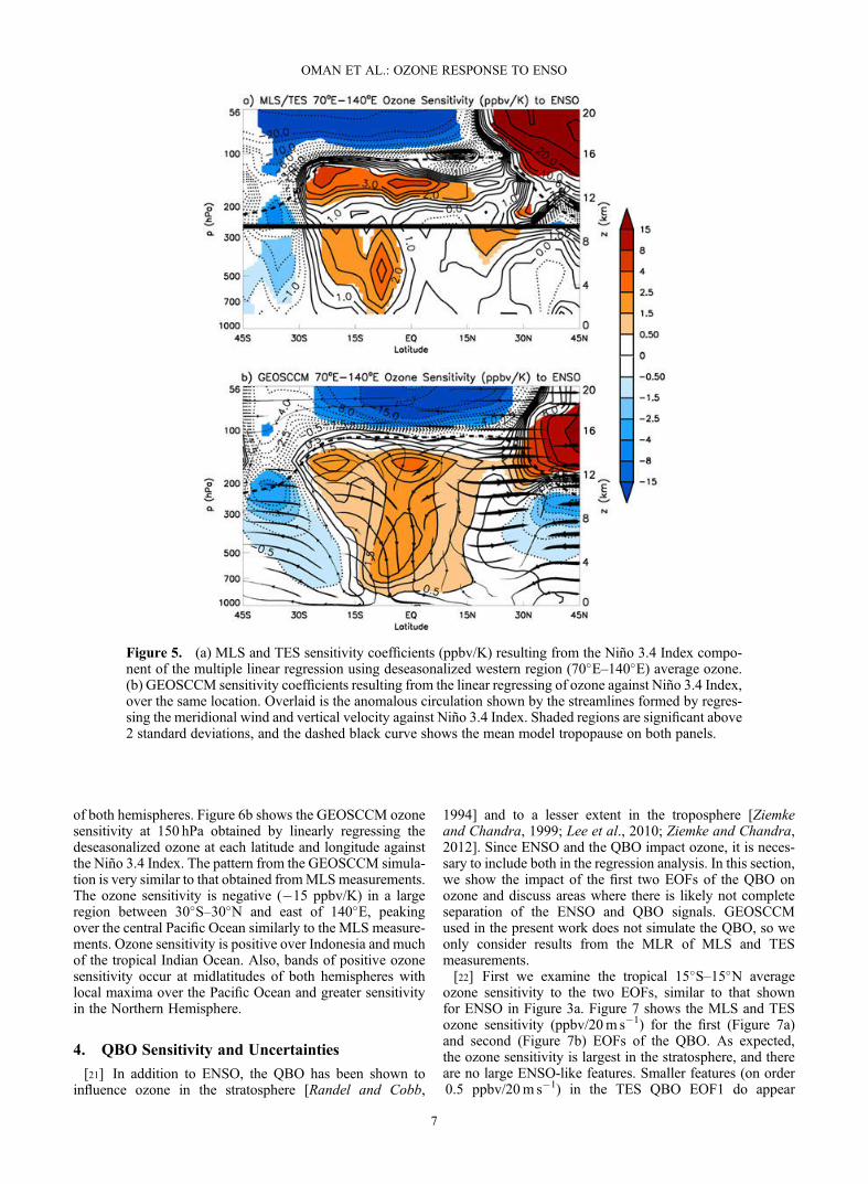
(70�E–140�E), shown in Figure 5, differs substantially fromthat in the eastern region. Figure 5 shows the ozone sensitiv-ity derived from (a) MLS and TES measurements and(b) GEOSCCM. Both the measurements and the model showa positive ozone response in the tropical troposphere and anegative ozone response in the tropical stratosphere like thatseen in the eastern region. The simulation shows anomalousdownwelling over the deep tropical troposphere, again con-sistent with observed circulation response to ENSO [Quanet al., 2004] and associated positive ozone sensitivitythroughout the deep tropical troposphere. There are threelocal maxima, one in the mid-troposphere from 10�S-Eq.and the other two in the upper troposphere, near the equatorand 20�S. Ozone sensitivity in the extratropical troposphereis generally negative. The lower stratospheric response ismore asymmetric than that seen in the eastern region, where


5

ozone sensitivity in the Northern Hemisphere midlatitudes ispositive between 30� and 45�.[19] Chandra et al. [1998] suggested that downward

motion, suppressed convection, and a drier troposphere allcontributed to the increase in ozone seen over the tropicalwestern Pacific and Indonesian region. The combination ofdownward motion and suppressed convection allows higherozone concentrations from the upper troposphere to be trans-ported downward [Sudo and Takahashi, 2001] and reducesthe upward transport of low ozone air over ocean surfaces.The drier troposphere also increases the chemical lifetimeof ozone, which causes increased tropospheric ozone concen-trations [Kley et al., 1996]. The ozone changes seen inFigure 5 in both simulation and measurements are consistentin sign with those expected from these previous studies. Overthe extratropical troposphere, the ozone sensitivity derivedfrom observations is negative in the Southern Hemisphere.The sensitivity derived from observations is asymmetric inthe midlatitude lower stratosphere and similar to that derived

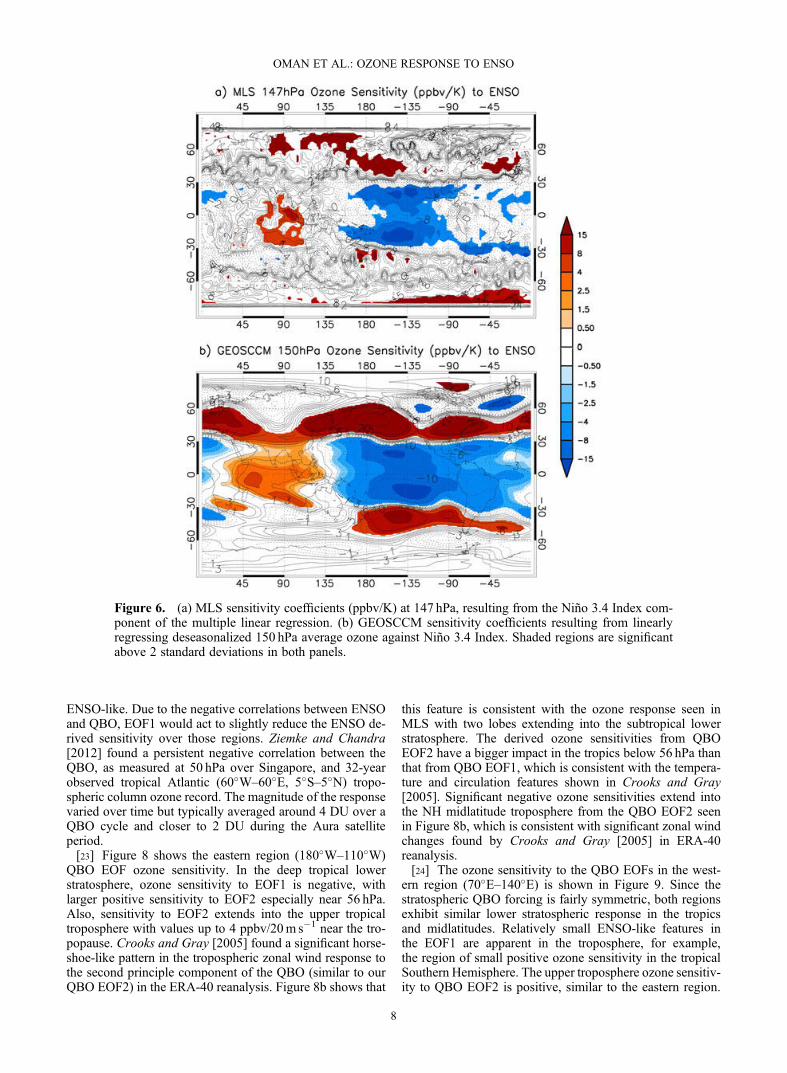
from GEOSCCM, with negative sensitivity in the SouthernHemisphere and positive in the Northern Hemisphere. TheGMI simulation including biomass-burning variability doesshow a larger ozone response in the tropical troposphere thanGEOSCCM and typically is in closer agreement with MLS/TES observations. This indicates that inter-annual variabilityin biomass burning does contribute to ozone variability inthis region.[20] We also examined the 150 hPa level globally to com-

pare variations in the pattern of horizontal ozone sensitivity.Figure 6a shows the ozone sensitivity derived from MLSmeasurements at 147 hPa using MLR. Over the tropicalPacific and Atlantic Oceans, negative ozone sensitivity dom-inates with dual local minima over the central Pacific of�15 ppbv/K approximately 15–20� off the equator in eachhemisphere. These anomalies are strongly influenced by theincreased horizontal poleward flow as shown in Figure 4b.Positive ozone sensitivity is seen over much of the tropicalIndian Ocean and in bands across much of the midlatitudes

Figure 4. (a) MLS and TES sensitivity coefficients (ppbv/K) resulting from the Niño 3.4 Index compo-nent of the multiple linear regression using deseasonalized eastern region (180�W–110�W) average ozone.(b) GEOSCCM sensitivity coefficients resulting from the linear regressing of ozone against Niño 3.4Index, over the same location. Overlaid is the anomalous circulation shown by the streamlines formedby regressing the meridional wind and vertical velocity against Niño 3.4 Index. Shaded regions are sig-nificant above 2 standard deviations, and the dashed black curve shows the mean model tropopause onboth panels.


6

of both hemispheres. Figure 6b shows the GEOSCCM ozonesensitivity at 150 hPa obtained by linearly regressing thedeseasonalized ozone at each latitude and longitude againstthe Niño 3.4 Index. The pattern from the GEOSCCM simula-tion is very similar to that obtained fromMLSmeasurements.The ozone sensitivity is negative (�15 ppbv/K) in a largeregion between 30�S–30�N and east of 140�E, peakingover the central Pacific Ocean similarly to the MLS measure-ments. Ozone sensitivity is positive over Indonesia and muchof the tropical Indian Ocean. Also, bands of positive ozonesensitivity occur at midlatitudes of both hemispheres withlocal maxima over the Pacific Ocean and greater sensitivityin the Northern Hemisphere.

4. QBO Sensitivity and Uncertainties

[21] In addition to ENSO, the QBO has been shown toinfluence ozone in the stratosphere [Randel and Cobb,

1994] and to a lesser extent in the troposphere [Ziemkeand Chandra, 1999; Lee et al., 2010; Ziemke and Chandra,2012]. Since ENSO and the QBO impact ozone, it is neces-sary to include both in the regression analysis. In this section,we show the impact of the first two EOFs of the QBO onozone and discuss areas where there is likely not completeseparation of the ENSO and QBO signals. GEOSCCMused in the present work does not simulate the QBO, so weonly consider results from the MLR of MLS and TESmeasurements.[22] First we examine the tropical 15�S–15�N average

ozone sensitivity to the two EOFs, similar to that shownfor ENSO in Figure 3a. Figure 7 shows the MLS and TESozone sensitivity (ppbv/20m s�1) for the first (Figure 7a)and second (Figure 7b) EOFs of the QBO. As expected,the ozone sensitivity is largest in the stratosphere, and thereare no large ENSO-like features. Smaller features (on order0.5 ppbv/20m s�1) in the TES QBO EOF1 do appear

Figure 5. (a) MLS and TES sensitivity coefficients (ppbv/K) resulting from the Niño 3.4 Index compo-nent of the multiple linear regression using deseasonalized western region (70�E–140�E) average ozone.(b) GEOSCCM sensitivity coefficients resulting from the linear regressing of ozone against Niño 3.4 Index,over the same location. Overlaid is the anomalous circulation shown by the streamlines formed by regres-sing the meridional wind and vertical velocity against Niño 3.4 Index. Shaded regions are significant above2 standard deviations, and the dashed black curve shows the mean model tropopause on both panels.


7

ENSO-like. Due to the negative correlations between ENSOand QBO, EOF1 would act to slightly reduce the ENSO de-rived sensitivity over those regions. Ziemke and Chandra[2012] found a persistent negative correlation between theQBO, as measured at 50 hPa over Singapore, and 32-yearobserved tropical Atlantic (60�W–60�E, 5�S–5�N) tropo-spheric column ozone record. The magnitude of the responsevaried over time but typically averaged around 4 DU over aQBO cycle and closer to 2 DU during the Aura satelliteperiod.[23] Figure 8 shows the eastern region (180�W–110�W)

QBO EOF ozone sensitivity. In the deep tropical lowerstratosphere, ozone sensitivity to EOF1 is negative, withlarger positive sensitivity to EOF2 especially near 56 hPa.Also, sensitivity to EOF2 extends into the upper tropicaltroposphere with values up to 4 ppbv/20m s�1 near the tro-popause. Crooks and Gray [2005] found a significant horse-shoe-like pattern in the tropospheric zonal wind response tothe second principle component of the QBO (similar to ourQBO EOF2) in the ERA-40 reanalysis. Figure 8b shows that

this feature is consistent with the ozone response seen inMLS with two lobes extending into the subtropical lowerstratosphere. The derived ozone sensitivities from QBOEOF2 have a bigger impact in the tropics below 56 hPa thanthat from QBO EOF1, which is consistent with the tempera-ture and circulation features shown in Crooks and Gray[2005]. Significant negative ozone sensitivities extend intothe NH midlatitude troposphere from the QBO EOF2 seenin Figure 8b, which is consistent with significant zonal windchanges found by Crooks and Gray [2005] in ERA-40reanalysis.[24] The ozone sensitivity to the QBO EOFs in the west-

ern region (70�E–140�E) is shown in Figure 9. Since thestratospheric QBO forcing is fairly symmetric, both regionsexhibit similar lower stratospheric response in the tropicsand midlatitudes. Relatively small ENSO-like features inthe EOF1 are apparent in the troposphere, for example,the region of small positive ozone sensitivity in the tropicalSouthern Hemisphere. The upper troposphere ozone sensitiv-ity to QBO EOF2 is positive, similar to the eastern region.

Figure 6. (a) MLS sensitivity coefficients (ppbv/K) at 147 hPa, resulting from the Niño 3.4 Index com-ponent of the multiple linear regression. (b) GEOSCCM sensitivity coefficients resulting from linearlyregressing deseasonalized 150 hPa average ozone against Niño 3.4 Index. Shaded regions are significantabove 2 standard deviations in both panels.


8

Lee et al. [2010] discussed finding ozone anomalies due tothe QBO in SHADOZ measurements of up to 8 ppbv in theupper troposphere. This size anomaly is consistent with theQBO EOF2 ozone sensitivity of 4 ppbv/20m s�1 found hereusing MLS measurements since the EOF2 typically variesbetween �40m/s (shown in Figure 1) over a typical QBOcycle.[25] As mentioned in section 2, the negative correlation

between ENSO and QBO EOF1 makes complete separationof the forcings using MLR not possible. Extending the obser-vational record would improve the separation of atmosphericprocesses if the correlation decreased with additional years.Unfortunately, TES did not make sufficient measurementsto produce meaningful monthly mean fields after January2010. Additionally, the use of multiple linear regressionwould not allow the representation of any nonlinear ozoneresponses. Hoerling et al. [1997] showed that differences in

the teleconnections do occur between El Nino and La Ninamost notably in the midlatitudes.[26] Other factors such as the strength of the Brewer-Dobson

circulation also play a role in the ozone concentrations in theUT/LS [Randel et al., 2007]. If these circulation changes aredue to ENSO [Calvo et al., 2010] or the QBO [Baldwin et al.,2001], they should be represented in this regression analysis;however, other factors not considered here could also impactthe strength of this circulation. Solar cycle variations couldalso impact lower atmospheric ozone [Chandra et al., 1999];however, due to the relative shortness of the observationalrecord compared to the length of a solar cycle, it is notincluded in this analysis. MLR tests which include a measureof solar cycle variability did not appear to significantly

Figure 7. MLS and TES sensitivity coefficients (ppbv/20m s�1) from the multiple linear regression analysis usingdeseasonalized tropical (15�S–15�N) average ozone for thefirst (a) and second (b) EOF of the QBO. Shaded regionsare significant above 2 standard deviations in both panels.

Figure 8. MLS and TES sensitivity coefficients (ppbv/20m s�1) from the multiple linear regression analysis usingdeseasonalized eastern region (180�W–110�W) averageozone for the first (a) and second (b) EOF of the QBO.Shaded regions are significant above 2 standard deviationsin both panels.


9

impact the derived ENSO and QBO ozone sensitivities. Also,excluding the QBO from the regression analysis does notsignificantly change the ENSO derived ozone response butdoes increase the uncertainty since the autocorrelation isincreased in the residual term.

5. Discussion and Conclusions

[27] This study presents observations of the response ofozone to ENSO from the lower troposphere to the lowerstratosphere and compares the response derived from obser-vations with that obtained from a GEOSCCM simulation.

We use a combination of MLS and TES measurements fromthe Aura satellite platform to derive the ozone response fromthe troposphere to the lower stratosphere. ENSO variationsare a dominant driver of tropical Pacific upper troposphericozone variability.[28] The tropical tropospheric ozone sensitivity to ENSO

is negative over much of Pacific and Atlantic Oceans andpositive over Indonesia and the Indian Ocean. This resultis seen in MLS and TES measurements and reproduced bythe GEOSCCM forced with observed sea-surface tempera-tures. Ozone sensitivity to ENSO is negative in the tropicallower stratosphere over all longitudes.[29] The eastern regional (180�W–110�W) ozone sensitivity

from both simulation and measurements is negative in thetropics and is larger in the upper troposphere and lowerstratosphere. Ozone sensitivity is positive over the midlati-tudes in the upper troposphere and lower stratosphere in mea-surements and simulations. There is excellent continuity inthe ozone response to ENSO derived from MLS and TESmeasurements near 261 hPa.[30] The western regional (70�E–140�E) response with

positive ozone sensitivity over the tropical troposphere isseen in GEOSCCM and measurements as well as negativesensitivity in the tropical lower stratosphere. In the lowerstratosphere midlatitudes, an asymmetric response is pro-duced in simulation and measurements, where negativeozone sensitivity occurs in the Southern Hemisphere andpositive ones in the Northern Hemisphere.[31] GEOSCCM reproduces the horizontal pattern and

response magnitude at around 150 hPa as derived from MLSmeasurements. The results presented here showing a tropicalupper tropospheric QBO-induced ozone change in MLSmeasurements are consistent with the findings of Lee et al.[2010] using the SHADOZ ozonesonde record.[32] This work shows a clear ozone response to ENSO

that is observed in MLS/TES measurements and can bereproduced in a GEOSCCM simulation; however, some dif-ferences are seen. A GMI simulation that includes biomass-burning variability does reduce some of the differencesbetween GEOSCCM and observations, especially overIndonesia. Some differences are also seen over SouthAmerica but are not significant in the observed ozone sensi-tivity to ENSO. Examining the response from atmosphericprocesses such as ENSO represents an excellent test forCCMs. It requires the proper simulation of horizontal andvertical gradients of ozone in the lower atmosphere alongwith the appropriate dynamical representation of a large-scale atmospheric process like ENSO. Tests such as thesecould provide a useful tool in the evaluation of CCMs. Con-tinued work needs to be done to determine if the response oftropospheric ozone to ENSO is useful for understandingprediction of ozone evolution. Changes in the frequency,magnitude, or type of ENSO could impact troposphericcomposition. Such changes in ENSO could result fromclimate change or could be important on decadal timescales through the Pacific Decadal Oscillation.

[33] Acknowledgments. This research was supported by the NASAMAP, ACMAP, and Aura programs. We would like to thank StaceyFrith for helping with the model output processing, Jacquie Witte andMike Manyin for the help with the measurement data sets, Feng Li forthe comments on an early version of this manuscript, and the three

Figure 9. MLS and TES sensitivity coefficients (ppbv/20m s�1) from the multiple linear regression analysis usingdeseasonalized western region (70�E–140�E) average ozonefor the first (a) and second (b) EOF of the QBO. Shadedregions are significant above 2 standard deviations in bothpanels.


10

anonymous reviewers for their very helpful comments. We also thankthose involved in model development at GSFC and the high-performancecomputing resources that were provided by NASA’s Advanced Supercom-puting Division.

ReferencesBaldwin, M. P., et al. (2001), The quasi-biennial oscillation, Rev. Geophys.,39(2), 179–229, doi:10.1029/1999RG000073.

Bjerknes, J. (1969), Atmospheric teleconnections from the equatorialPacific, Mon. Weather Rev., 18, 820–829.

Calvo, N., R. R. Garcia, W. J. Randel, and D. Marsh (2010), Dynamicalmechanism for the increase in tropical upwelling in the lowermosttropical stratosphere during warm ENSO events, J. Atmos. Sci., 67,2331–2340.

Chandra, S., J. R. Ziemke, W. Min, and W. G. Read (1998), Effects of1997–1998 El Niño on tropospheric ozone and water vapor, Geophys.Res. Lett., 25, 3867–3870.

Chandra, S., J. R. Ziemke, and R. W. Stewart (1999), An 11-year solar cyclein tropospheric ozone from TOMS measurements, Geophys. Res. Lett.,26(2), 185–188, doi:10.1029/1998GL900272.

Chandra, S., J. R. Ziemke, P. K. Bhartia, and R. V. Martin (2002), Tropicaltropospheric ozone: Implications for dynamics and biomass burning,J. Geophys. Res., 107(D14), 4188, doi:10.1029/2001JD000447.

Chandra, S. J. R. Ziemke, B. N. Duncan, T. L. Diehl, N. J. Livesey, and L.Froidevaux (2009), Effects of the 2006 El Niño on tropospheric ozoneand carbon monoxide: Implications for dynamics and biomass burning,Atmos. Chem. Phys., 9, 4239–4249.

Crooks, S. A., and L. J. Gray (2005), Characterization of the 11-yearsolar signal using a multiple regression analysis of the ERA-40 dataset,J. Clim., 18, 996–1015.

Doherty, R. M., D. S. Stevenson, C. E. Johnson, W. J. Collins, and M. G.Sanderson (2006), Tropospheric ozone and El Niño–Southern Oscillation:Influence of atmospheric dynamics, biomass burning emissions, andfuture climate change, J. Geophys. Res., 111, D19304, doi:10.1029/2005JD006849.

Duncan, B. N., S. E. Strahan, Y. Yoshida, S. D. Steenrod, and N. Livesey,(2007), Model study of the cross-tropopause transport of biomass burningpollution, Atmos. Chem. Phys., 7, 3713–3736.

Enfield, D. B. (1989), El Niño, past and present, Rev. Geophys., 27(1),159–187, doi:10.1029/RG027i001p00159.

Eyring, V., et al. (2005), A strategy for process-oriented validation of coupledchemistry-climate models, Bull. Am. Meteorol. Soc., 86, 1117–1133.

Haigh, J. D., M. Blackburn, and R. Day (2005), The response of tropo-spheric circulation to perturbations in lower-stratospheric temperature.J. Clim., 18, 3672–3685.

Hoerling, M. P., A. Kumar, and M. Zhong (1997), El Niño, La Niña, and thenonlinearity of their teleconnections, J. Clim., 10, 1769–1786.

Jacobson, M. Z. (1995), Computation of global photochemistry withSMVGEAR II, Atmos. Environ., 29, 2541–2546.

Kley, D., P. J. Crutzen, H. G. J. Smit, H. Vomel, S. J. Oltmans, H. Grassl, andV. Ramanathan (1996), Observations of near-zero ozone concentrationsover the convective Pacific: Effects on air chemistry, Science, 274, 230–233.

Lang, C., D.W.Waugh, M. A. Olsen, A. R. Douglass, Q. Liang, J. E. Nielsen,L. D. Oman, S. Pawson, and R. S. Stolarski (2012), The impact ofgreenhouse gases on past changes in tropospheric ozone, J. Geophys.Res., 117, D23304, doi:10.1029/2012JD018293.

Langford, A. O., T. J. O’Leary, C. D. Masters, K. C. Aikin, andM. H. Proffitt(1998), Modulation of middle and upper tropospheric ozone at Northernmidlatitudes by the El Niño/Southern Oscillation, Geophys. Res. Lett.,25, 2667–2670.

Langford, A. O. (1999), Stratosphere-troposphere exchange at the subtrop-ical jet: contribution to the tropospheric ozone budget at midlatitudes,Geophys. Res. Lett., 26, 2449–2452.

Lee, S., D. M. Shelow, A. M. Thompson, and S. K. Miller (2010), QBO andENSO variability in temperature and ozone from SHADOZ, 1998–2005,J. Geophys. Res., 115, D18105, doi:10.1029/2009JD013320.

Livesey, N. J., et al. (2011), Earth Observing System (EOS) Aura Micro-wave Limb Sounder (MLS) version 3.3 level 2 data quality and descrip-tion document, JPL D-33509, Jet Propulsion Laboratory, California Insti-tute of Technology, Pasadena, California, USA, 162 pp.

Logan, J. A., I. Megretskaia, R. Nassar, L. T. Murray, L. Zhang, K. W.Bowman, H. M. Worden, and M. Luo (2008), Effects of the 2006 El Ninoon tropospheric composition as revealed by data from the TroposphericEmission Spectrometer (TES), Geophys. Res. Lett., 35, L03816,doi:10.1029/2007GL031698.

Nassar, R., et al. (2008), Validation of Tropospheric Emission Spectrometer( TES) nadir ozone profiles using ozonesonde measurements, J. Geophys.Res., 113, D15S17, doi:10.1029/2007JD008819.

Nassar, R., J. A. Logan, I. A. Megretshaia, L. T. Murray, L. Zhang,and D. B. A. Jones (2009), Analysis of tropical tropospheric ozone,carbon monoxide, and water vapor during the 2006 El Nino usingTES observations and the GEOS-Chem model, J. Geophys. Res.,114, D17304, doi:10.1029/2009JD011760.

Oman, L., D. W. Waugh, S. R. Kawa, R. S. Stolarski, A. R. Douglass, andP. A. Newman (2009), Mechanisms and feedbacks causing changes inupper stratospheric ozone in the 21st century, J. Geophys. Res., 114,doi:10.1029/2009JD012397.

Oman, L. D., et al. (2010), Multimodel assessment of the factors drivingstratospheric ozone evolution over the 21st century, J. Geophys. Res.,115, D24306, doi:10.1029/2010JD014362.

Oman, L. D., J. R. Ziemke, A. R. Douglass, D. W. Waugh, C. Lang,J. M. Rodriguez, J. E. Nielsen (2011), The response of tropicaltropospheric ozone to ENSO, Geophys. Res. Lett., 38, doi:10.1029/2011GL047865.

Peters, W., M. Krol, F. Dentener, and J. Lelieveld (2001), Identification ofan El Nino Southern Oscillation signal in a multiyear global simulationof tropospheric ozone. J. Geophys. Res., 106, 10,389–10,402.

Philander, S. G. (1989), El Niño, La Nina, and the Southern Oscillation,pp. 293, Academic Press, San Diego, California, United States.

Quan, X.-W., H. F. Diaz, and M. P. Hoerling (2004), Change in the tropicalHadley cell since 1950, in The Hadley Circulation: Past, Present, andFuture, edited by H. F. Diaz and R. S. Bradley, Cambridge Univ. Press,New York.

Randel, W. J., and J. B. Cobb (1994), Coherent variations of monthly meantotal ozone and lower stratospheric temperature. J. Geophys. Res., 99,5433–5477.

Randel, W. J., M. Park, F. Wu, and N. Livesey (2007), A large annual cyclein ozone above the tropical tropopause linked to the Brewer-Dobson cir-culation, J. Atmos. Sci., 64, 4479–4488.

Randel, W. J., R. R. Garcia, N. Calvo, and D. Marsh (2009), ENSO influenceon zonal mean temperature and ozone in the tropical lower stratosphere,Geophys. Res. Lett., 36, L15822, doi:10.1029/2009GL039343.

Randel, W. J., and A. M. Thompson (2011), Interannual variability andtrends in tropical ozone derived from SAGE II satellite data andSHADOZ ozonesondes, J. Geophys. Res., 116, D07303, doi:10.1029/2010JD015195.

Rayner, N. A., D. E. Parker, E. B. Horton, C. K. Folland, L. V. Alexander,D. P. Rowell, E. C. Kent, and A. Kaplan (2003), Global analyses of seasurface temperature, sea ice, and night marine air temperature since thelate nineteenth century, J. Geophys. Res., 108(D14), 4407, doi:10.1029/2002JD002670.

Rienecker, M. M., et al. (2008), The GEOS-5 data assimilation system—Documentation of versions 5.0.1, 5.1.0, and 5.2.0. Technical ReportSeries on Global Modeling and Data Assimilation, 27.

SPARC CCMVal (2010), SPARC Report on the Evaluation of Chemistry-Climate Models, V. Eyring, T. G. Shepherd, D. W. Waugh (Eds.), SPARCReport No. 5, WCRP-132, WMO/TD-No. 1526, http://www.atmosp.physics.utoronto.ca/SPARC.

Stolarski, R. S., P. Bloomfield, R. D. McPeters, and J. R. Herman (1991),Total ozone trends deduced from Nimbus-7 TOMS data, Geophys. Res.Lett., 18, 1015–1018.

Stolarski, R. S., A. R. Douglass, S. Steenrod, and S. Pawson (2006), Trendsin stratospheric ozone: Lessons learned from a 3D chemical transportmodel, J. Atmos. Sci., 63, 1028–1041.

Strahan, S. E., B. N. Duncan and P. Hoor (2007), Observationally-deriveddiagnostics of transport in the lowermost stratosphere and their applica-tion to the GMI chemistry transport model, Atmos. Chem. Phys., 7,2435–2445.

Strahan, S. E., et al. (2011), Using transport diagnostics to understandchemistry climate model ozone simulations, J. Geophys. Res., 116,D17302, doi:10.1029/2010JD015360.

Sudo, K., M. Takahashi (2001), Simulation of tropospheric ozone changesduring 1997–1998 El Niño: Meteorological impact on troposphericphotochemistry, Geophys. Res. Lett., 28, 4091–4094.

Tiao, G., G. Reinsel, D. Xu, J. Pedrick, X. Zhu, A. Miller, J. DeLuisi,C. Mateer, and D. Wuebbles (1990), Effects of autocorrelationand temporal sampling schemes on estimates of trend and spatialcorrelation, J. Geophys. Res., 95(D12), 20,507–20,517, doi:10.1029/JD095iD12p20507.

Voulgarakis, A., P. Hadjinicolaou, and J. A. Pyle (2011), Increases in globaltropospheric ozone following an El Niño event: Examining stratosphericozone variability as a potential driver, Atmos Sci Let., 12, doi: 10.1002/asl.318.

Wallace, J. M., R. L. Panetta, and J. Estberg (1993), Representation of theequatorial stratospheric quasi-biennial oscillation in EOF phase space,J. Atmos. Sci., 50, 1751–1762.

Zeng, G., and J. A. Pyle (2005), Influence of El Niño Southern Oscillationon stratosphere/troposphere exchange and the global tropospheric


11

ozone budget, Geophys. Res. Lett., 32, L0814, doi:10.1020/2004GL021353.

Ziemke, J. R., and S. Chandra (1999), Seasonal and inter-annual variabilitiesin tropical tropospheric ozone, J. Geophys. Res., 104, 21,425–21,442.

Ziemke, J. R., and S. Chandra (2003), La Nina and El Niño-induced vari-abilities of ozone in the tropical lower atmosphere during 1970–2001,Geophys. Res. Lett., 30, 1142, doi:10.1029/2002GL016387.

Ziemke, J. R., S. Chandra, L. D. Oman, and P. K. Bhartia (2010), A newENSO index derived from satellite measurements of column ozone,Atm. Chem. Phys., 10, 3711–3721.

Ziemke, J. R., and S. Chandra (2012), Development of a climate record oftropospheric and stratospheric ozone from satellite remote sensing:Evidence of an early recovery of global stratospheric ozone, Atmos. Chem.Phys., 12, 5737–5753, doi:10.5194/acp-12-5737-2012.


12

the ozone response to enso in aura satellite measurements...

Documents