the overprediction of liquefaction hazard in certain … · the overprediction of liquefaction...
TRANSCRIPT
THE OVERPREDICTION OF
LIQUEFACTION HAZARD IN
CERTAIN AREAS OF LOW TO
MODERATE SEISMICITYDr. Kevin Franke, Ph.D., P.E., M.ASCE
Dept. of Civil and Environmental Engineering
Brigham Young University
April 20, 2017

Liquefaction Hazard
Liquefaction can result in significant damage to infrastructure during earthquakes
Liquefaction hazard is generally correlated with seismic hazard
Some areas of low to moderate seismicity have significant liquefaction hazard, however
Image: Karl V. Steinbrugge Collection, EERC, Univ
of California, Berkeley

Overview of Simplified Empirical
Method
Liquefaction is usually evaluated with a factor of safety,
FSL
Resistance Cyclic Resistance Ratio
Loading Cyclic Stress RatioL
CRRFS
CSR
Liq
No Liq
(after Mayfield et al. 2010)
Function of both amax
and Mw, which
collectively characterize
seismic loading
CSR
siteCSR
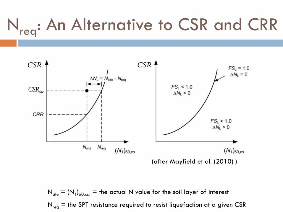
Nreq: An Alternative to CSR and CRR
Nsite = (N1)60,cs,i = the actual N value for the soil layer of interest
Nreq = the SPT resistance required to resist liquefaction at a given CSR
(after Mayfield et al. (2010) )
CSR
siteCSR
CSR

Various Approaches for Liquefaction
Hazard Analysis
Deterministic Approach
Pseudo-Probabilistic Approach
Probabilistic (or Performance-Based) Approach
• Considers an individual seismic source and corresponding ground
motions individually
• Usually assumes mean values for the inputs and models
• Considers probabilistic ground motion from a single return period
• Usually assumes mean values for the inputs and models
• Considers probabilistic ground motions from ALL return periods
• Accounts for parametric and model uncertainties
• Results depend on desired hazard level or return period
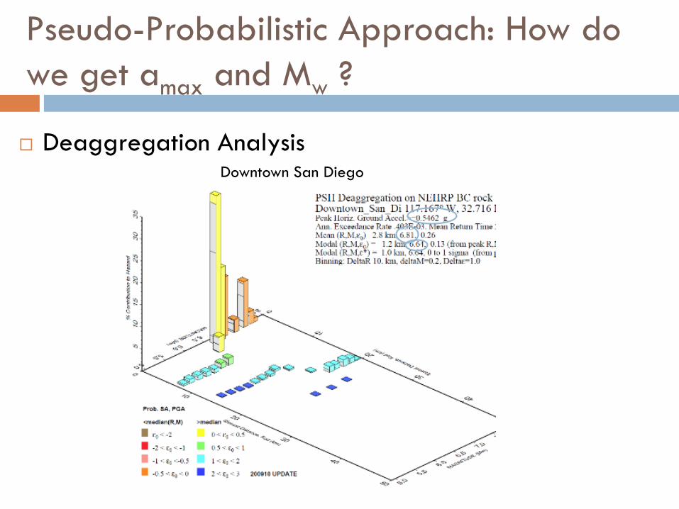
Pseudo-Probabilistic Approach: How do
we get amax and Mw ?
Deaggregation AnalysisDowntown San Diego

Conventional (i.e., “pseudo-probabilistic”)
Liquefaction Triggering Procedure
1. Perform PSHA with PGA and a deaggregation analysis at the
specified return period of PGA (e.g., 2475-year for the MCE)
2. Obtain either the mean or modal Mw from the deaggregation
analysis
3. Correct the PGA value for site response using site amplification
factors or a site response analysis to compute amax
4. Couple amax with the mean or modal Mw to perform a scenario
liquefaction triggering analysis
5. Typically define liquefaction triggering as PL≥15% and FSL≤1.2

Pseudo-Probabilistic Example…..
Consider the following site in Cincinnati, Ohio:

Pseudo-Probabilistic Example…..
Here is the corresponding 2,475-yr deaggregation
from the USGS:
PGA = 0.067 g

Pseudo-Probabilistic Example…..
Consider the liquefaction triggering and settlement
results for a site in Cincinnati, Ohio:
Conventional Approach, MCEG with Modal Magnitude
Does this make sense? How likely is it that an M7.5 EQ over 450
km away produces PGA = 0.067g? <1% according to Toro et al. (1997)
<2% according to Atkinson and Boore (2006)

Challenges with the Pseudo-
probabilistic Approach
It can be easy to make an “incompatible” (amax, Mw) pair,
especially if using the modal Mw
PGA and Mw typically are taken from a single return
period, but other return periods are ignored
Does not rigorously account for uncertainty in the
liquefaction triggering model or the site response
Contributes to inaccurate interpretations of liquefaction
hazard (e.g., “I used the 2,475-year PGA in my analysis,
so my liquefaction results correspond to the 2,475-year
return period.”)
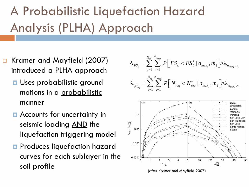
A Probabilistic Liquefaction Hazard
Analysis (PLHA) Approach
Kramer and Mayfield (2007)
introduced a PLHA approach
Uses probabilistic ground
motions in a probabilistic
manner
Accounts for uncertainty in
seismic loading AND the
liquefaction triggering model
Produces liquefaction hazard
curves for each sublayer in the
soil profile
max
maxmax ,
1 1
| ,aM
L i ji
NN
FS L L j a m
j i
P FS FS a m
max
maxmax ,
1 1
| ,aM
i jireq
NN
req req j a mNj i
P N N a m
(after Kramer and Mayfield 2007)

Back to the Cincinnati Example…..
Let’s use the Kramer and Mayfield (2007) PLHA approach
with the Boulanger and Idriss (2012) triggering model:
Conventional Approach, MCEG with Modal Magnitude PLHA Approach, Tr=2,475 years
Only difference: how we considered our seismic loading and
uncertainties!
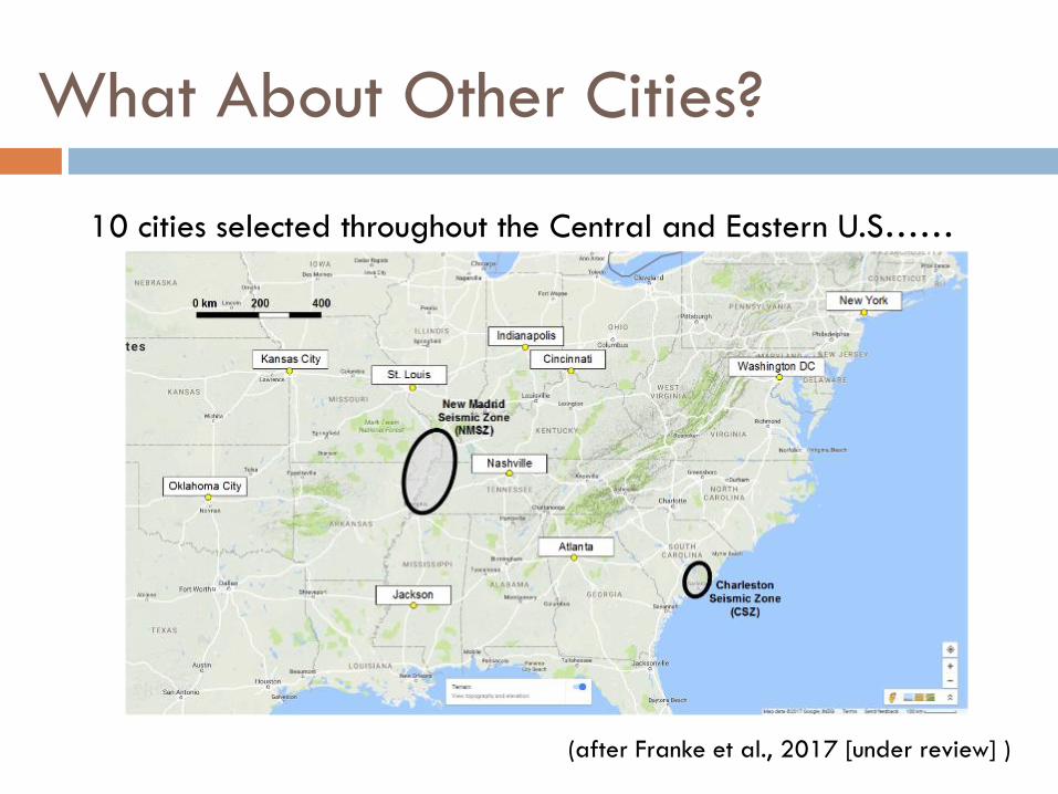
What About Other Cities?
10 cities selected throughout the Central and Eastern U.S……
(after Franke et al., 2017 [under review] )
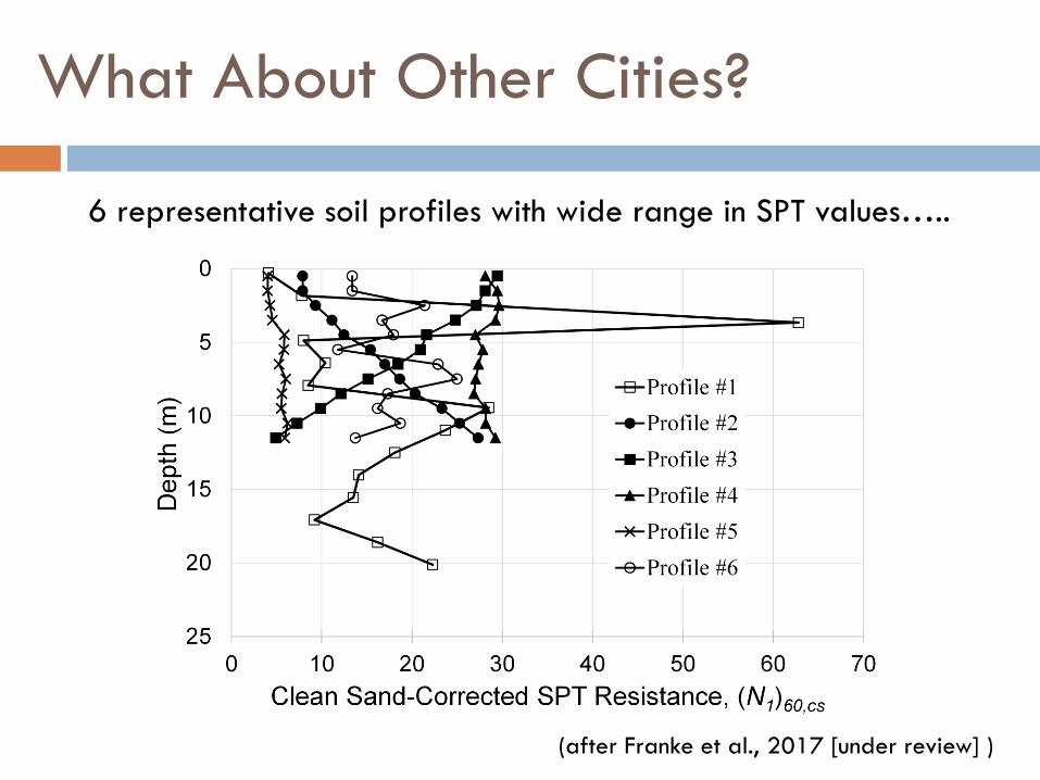
What About Other Cities?
6 representative soil profiles with wide range in SPT values…..
(after Franke et al., 2017 [under review] )

What About Other Cities?
Results if assuming a Site Class D…..
(after Franke et al., 2017 [under review] )
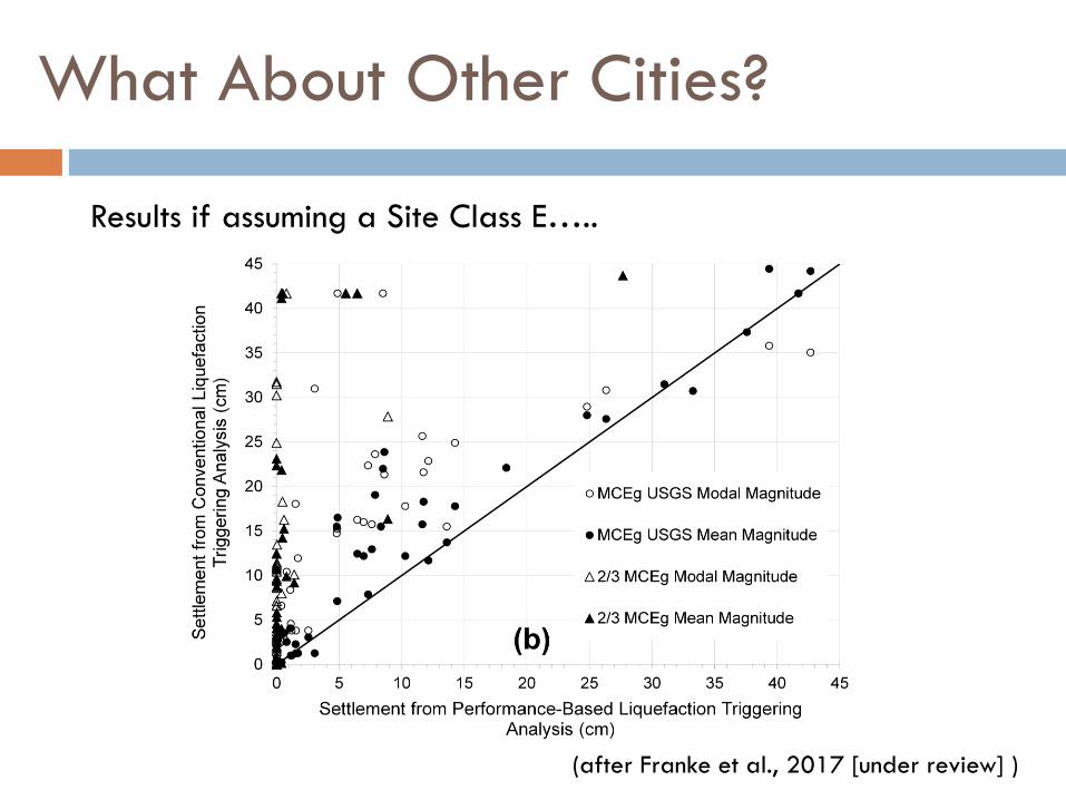
What About Other Cities?
Results if assuming a Site Class E…..
(after Franke et al., 2017 [under review] )

Existing Tools for PLHA Approach in
Practice
WSLiq (http://faculty.washington.edu/kramer/WSliq/WSliq.htm)
o Developed by the U. of Washington in 2008 using VB.Net
o Accounts for multiple liquefaction hazards (triggering, lateral spread, settlement, and residual strength)
o Developed only for use in Washington State with 2002 USGS ground motion data, but you can “trick” the program for other locations
o Limited control over the analysis uncertainty options and models
PBLiquefY v2.0
o V1.0 developed by BYU in 2013 using Microsoft Excel and VBA
o Liquefaction triggering, settlement, and Newmark slope displacement
o Compatible with USGS 1996, 2002, 2008, or 2014 ground motions.
o Can be used for any site in the U.S.
o Multiple model options
o Offers lots of control over the analysis uncertainties, including site amplification factors
Neither of these tools has been used widely in design!
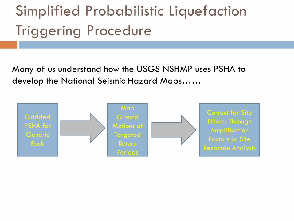
Simplified Probabilistic Liquefaction
Triggering Procedure
Many of us understand how the USGS NSHMP uses PSHA to
develop the National Seismic Hazard Maps……
Gridded
PSHA for
Generic
Rock
Correct for Site
Effects Through
Amplification
Factors or Site
Response Analysis
Map
Ground
Motions at
Targeted
Return
Periods

Mayfield et al. (2010) presented a similar idea for liquefaction
triggering….
Gridded
PB Analysis
for Generic
Soil Layer
Correct for
Site-Specific
Soil
Conditions
and Stresses
Map Liq
Hazard at
Targeted
Return
Periods
Liquefaction
Parameter Map
DIFFERENT
FROM a
Liquefaction
Hazard Map
Depth Reduction
Soil Stresses
Site Amplification
Simplified Probabilistic Liquefaction
Triggering Procedure
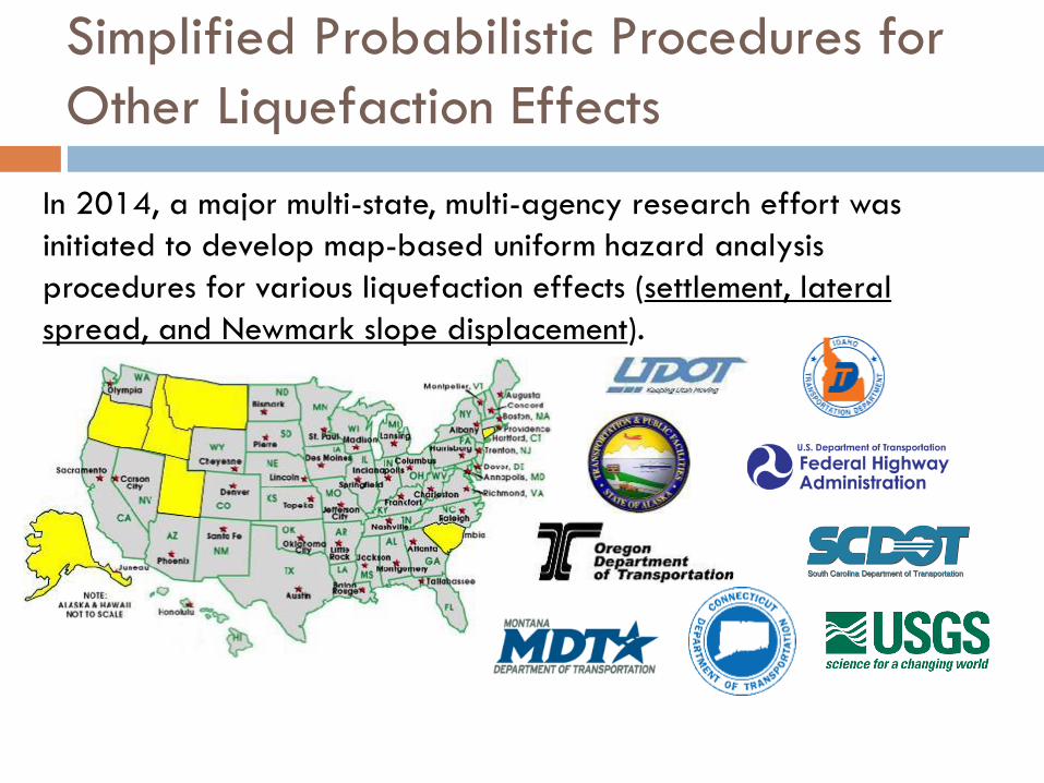
Simplified Probabilistic Procedures for
Other Liquefaction Effects
In 2014, a major multi-state, multi-agency research effort was
initiated to develop map-based uniform hazard analysis
procedures for various liquefaction effects (settlement, lateral
spread, and Newmark slope displacement).

Boulanger and Idriss (2012, 2014)
Simplified PB Liquefaction Model
Research was performed at BYU to develop a simplified
procedure for the Boulanger and Idriss (2012, 2014) probabilistic
triggering model. Similar to the approach introduced by Mayfield
et al. (2010), but we incorporated a few changes:
The quadratic equation format of the Boulanger and Idriss
model requires a different and more complex approach
Many engineers are still uncomfortable with the Nreq concept
Incorporation of the (N1)60,cs-dependent MSF
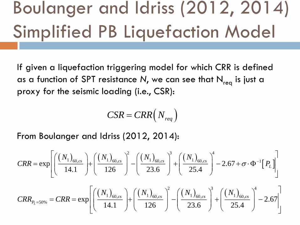
If given a liquefaction triggering model for which CRR is defined
as a function of SPT resistance N, we can see that Nreq is just a
proxy for the seismic loading (i.e., CSR):
From Boulanger and Idriss (2012, 2014):
reqCSR CRR N
2 3 4
1 1 1 160, 60, 60, 60, 1exp 2.6714.1 126 23.6 25.4
cs cs cs cs
L
N N N NCRR P
Boulanger and Idriss (2012, 2014)
Simplified PB Liquefaction Model
2 3 4
1 1 1 160, 60, 60, 60,
50% exp 2.6714.1 126 23.6 25.4L
cs cs cs cs
P
N N N NCRR CRR

By combining equations, we obtain:
2 3 4
50% exp 2.6714.1 126 23.6 25.4L
req req req req
P
N N N NCSR CSR
So instead of developing liquefaction parameter maps
for a reference Nreq, we can develop reference maps for
the median CSR to characterize seismic loading.
Engineers seem much more comfortable characterizing
seismic loading with CSR than they do with Nreq.
We have called these new maps Liquefaction Loading
Parameter Maps.
Boulanger and Idriss (2012, 2014)
Simplified PB Liquefaction Model
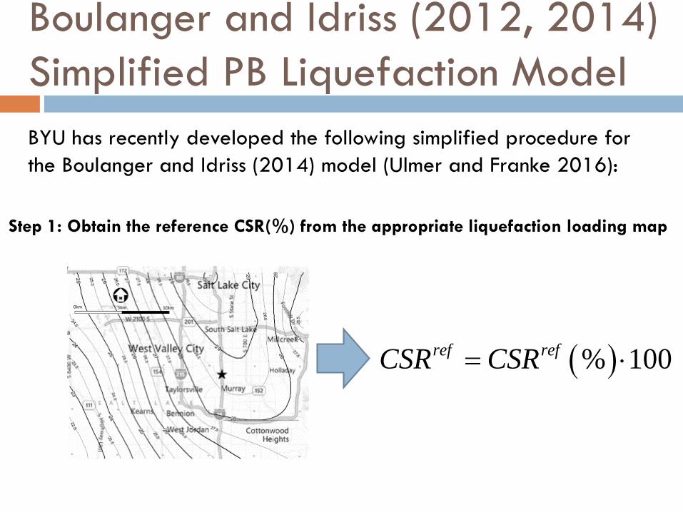
Step 1: Obtain the reference CSR(%) from the appropriate liquefaction loading map
% 100ref refCSR CSR
BYU has recently developed the following simplified procedure for
the Boulanger and Idriss (2014) model (Ulmer and Franke 2016):
Boulanger and Idriss (2012, 2014)
Simplified PB Liquefaction Model

BYU has recently developed the following simplified procedure for
the Boulanger and Idriss (2014) model (Ulmer and Franke 2016):
Step 2: For every soil sublayer in your profile, compute the appropriate CSR
correction factors, CSR
Site Amplification:
Depth Reduction:
(z in meters)
lnpgaF pgaCSR F
0.6712 1.126sin 5.133 0.0675 0.118sin 5.14211.73 11.28dr w
z zCSR M
Mean magnitude from PGA
deaggregation at target return
period
Soil Stress:
Boulanger and Idriss (2012, 2014)
Simplified PB Liquefaction Model

Step 2: For every soil sublayer in your profile, compute the appropriate CSR
correction factors, CSR
Duration:
max
max
1 1 8.64exp 1.3254
ln ln
1 1 8.64exp 1.3254
site w
site
MSF ref
ref w
MMSF
MSFCSR
MSF MMSF
2
1 60,
max 1.09 2.231.5
cssiteN
MSF
2
4 3 2
max
1.237 ln 4.918 ln 1.762 ln 5.473 ln 33.651.09 2.2
31.5
ref ref ref ref
refCSR CSR CSR CSR
MSF
BYU has recently developed the following simplified procedure for
the Boulanger and Idriss (2014) model (Ulmer and Franke 2016):
Boulanger and Idriss (2012, 2014)
Simplified PB Liquefaction Model
**NOTE: if you prefer MSF from Boulanger and Idriss (2012), then CSRMSF = 0 ***

Step 2: For every soil sublayer in your profile, compute the appropriate CSR
correction factors, CSR
Overburden:
'1 ln
ln ln'
1 ln
site
site v
sitea
K ref ref
ref v
a
CPK
CSRK
CP
1 60,
10.3
18.9 2.55
site
cs
CN
0.5
4 3 2
10 0.3
18.9 2.55 1.237 ln 4.918 ln 1.762 ln 5.473 ln 33.65
site
ref ref ref ref
C
CSR CSR CSR CSR
BYU has recently developed the following simplified procedure for
the Boulanger and Idriss (2014) model (Ulmer and Franke 2016):
Boulanger and Idriss (2012, 2014)
Simplified PB Liquefaction Model
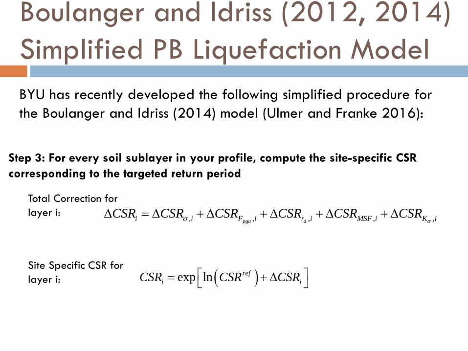
Step 3: For every soil sublayer in your profile, compute the site-specific CSR
corresponding to the targeted return period
Total Correction for
layer i:
Site Specific CSR for
layer i:
, , , , ,pga di i F i r i MSF i K iCSR CSR CSR CSR CSR CSR
exp ln ref
i iCSR CSR CSR
BYU has recently developed the following simplified procedure for
the Boulanger and Idriss (2014) model (Ulmer and Franke 2016):
Boulanger and Idriss (2012, 2014)
Simplified PB Liquefaction Model

Step 4: For each soil sublayer in your profile, characterize liquefaction triggering
hazard using whichever metric you prefer
Factor of Safety:
Probability of Liquefaction:
*Note that these equations account for both parametric uncertainty (e.g., (N1)60,cs ) and model
uncertainty, and are only to be used with the Boulanger and Idriss (2014) procedure.
2 3 4
1 1 1 160, 60, 60, 60,exp 2.67
14.1 126 23.6 25.4
cs cs cs csi i i i
iL i
i i
N N N N
CRRFS
CSR CSR
ln
ln
0.277 0.277
i
L ii
L i
CRR
CSR FSP
BYU has recently developed the following simplified procedure for
the Boulanger and Idriss (2014) model (Ulmer and Franke 2016):
Boulanger and Idriss (2012, 2014)
Simplified PB Liquefaction Model
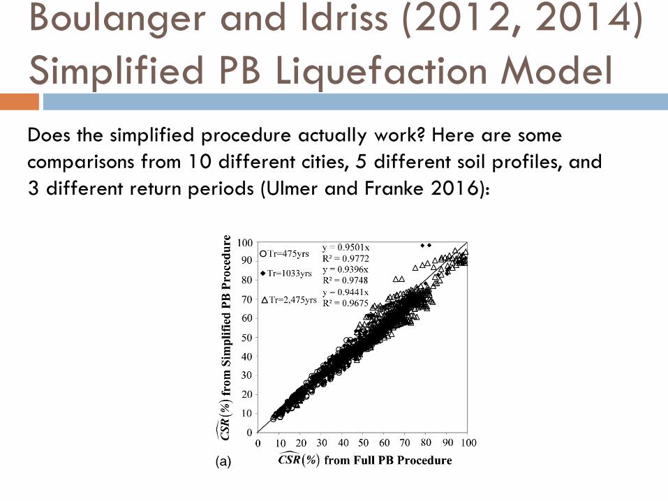
Does the simplified procedure actually work? Here are some
comparisons from 10 different cities, 5 different soil profiles, and
3 different return periods (Ulmer and Franke 2016):
Boulanger and Idriss (2012, 2014)
Simplified PB Liquefaction Model
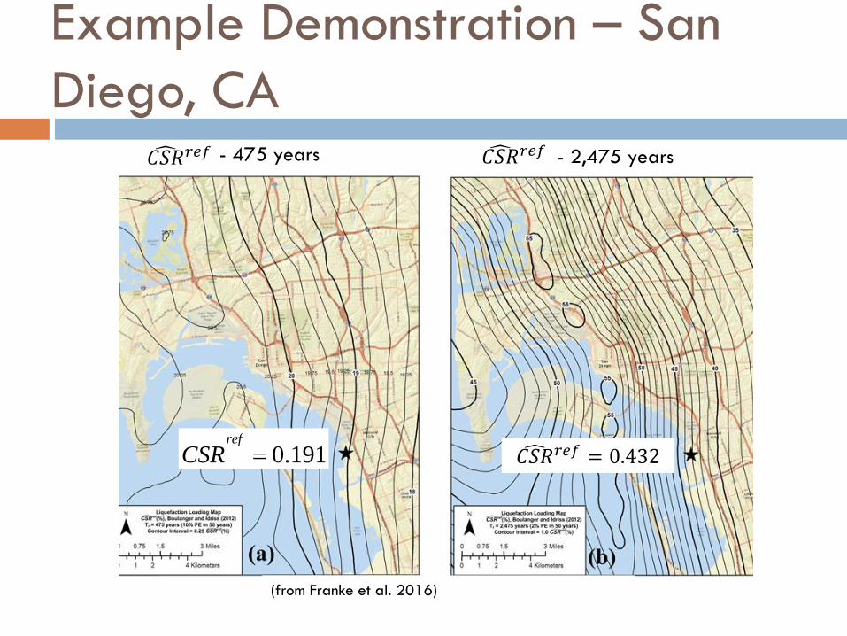
Example Demonstration – San
Diego, CA𝐶𝑆𝑅𝑟𝑒𝑓 - 475 years 𝐶𝑆𝑅𝑟𝑒𝑓 - 2,475 years
0.191ref
CSR 𝐶𝑆𝑅𝑟𝑒𝑓 = 0.432
(from Franke et al. 2016)

Example Demonstration – San
Diego, CA
Depth, z
(m) Soil Type Thickness (m)
(blows/0.3
meter)
Fines
(%)
Unit Weight
(kN/m3)
(blows/0.3
meter)
0.1 Hydraulic Fill 0.5 12 3 18.70 12.0
0.6 Hydraulic Fill 1.0 20 4 18.70 20.0
1.5 Poorly Graded Sand with Silt
0.5
28 11 18.85 33.6
2.1 Poorly Graded Sand with Silt
1.0
35 12 18.85 37.1
3 Silty Sand 1.5 36 15 19.55 39.3
4.6 Poorly Graded Sand with Silt
1.5
13 8 18.85 13.4
6.1 Poorly Graded Sand with Silt
1.5
14 6 18.85 14.0
7.6 Silty Sand 1.5 36 18 19.55 40.1
9.1 Silty Sand 1.5 43 20 19.55 47.5
10.7 Silty Sand 1.5 50+ 17 19.55 54+
12.2 Silty Sand 1.5 50+ 23 19.55 55+
13.7 Silty Sand 1.5 50+ 24 19.55 55+
15.2 Silty Sand 1.5 50+ 22 19.55 55+
1 Computed using Idriss and Boulanger [2008, 2010]
1 60N 1 60,cs
N
Groundwater at z = 2.0 metersFree-face case, W = 10%
𝐷50 15 = 0.5𝑚𝑚
(from Franke et al. 2016)

Example Demonstration – San
Diego, CA
1 60N 1 60,cs
N
Depth,
z (m) USCS
(N1)60,cs
(blows/0.3
meter)
CSR
Eqn A2)
pgaFCSR
Eqn A3)
drCSR
(Eqn A4)
KCSR
Eqn A5)
CSR
(Eqn A1)
475 (2,475) CRR 1
LiqFS
(Eqn A7)
475 (2,475)
Return Period
of
Liquefaction 2
(years)
1.5 SP-SM 33.6 -0.693 0.37 (0.07) 0.08 (0.07) -0.206 0.121 (0.203) >0.6 >2 (>2) >10,000
2.1 SP-SM 37.1 -0.532 0.37 (0.07) 0.07 (0.06) -0.219 0.139 (0.233) >0.6 >2 (>2) >10,000
3 SM 39.3 -0.399 0.37 (0.07) 0.05 (0.05) -0.164 0.166 (0.278) >0.6 >2 (>2) >10,000
4.6 SP-SM 13.4 -0.262 0.37 (0.07) 0.03 (0.03) 0.006 0.219 (0.368) 0.163 0.75 (0.44) 284
6.1 SP-SM 14.0 -0.196 0.37 (0.07) 0.00 (0.00) 0.026 0.232 (0.390) 0.168 0.73 (0.43) 232
7.6 SM 40.1 -0.174 0.37 (0.07) -0.03 (-0.03) 0.023 0.229 (0.386) >0.6 >2 (>2) >10,000
9.1 SM 47.5 -0.147 0.37 (0.07) -0.07 (-0.07) 0.068 0.238 (0.402) >0.6 >2 (>2) >10,000
10.7 SM 54 -0.125 0.37 (0.07) -0.11 (-0.10) 0.112 0.244 (0.413) >0.6 >2 (>2) >10,000
12.2 SM 54 -0.110 0.37 (0.07) -0.15 (-0.14) 0.149 0.247 (0.420) >0.6 >2 (>2) >10,000
13.7 SM 54 -0.098 0.37 (0.07) -0.19 (-0.18) 0.184 0.249 (0.423) >0.6 >2 (>2) >10,000
15.2 SM 54 -0.089 0.37 (0.07) -0.23 (-0.22) 0.216 0.249 (0.425) >0.6 >2 (>2) >10,000
1 Computed with Boulanger and Idriss [58], PL=50%
2 Computed with Kramer and Mayfield [5] procedure using
the Boulanger and Idriss [58] model
1 (from Franke et al. 2016)
Liquefaction Triggering Results (Ulmer and Franke 2016)
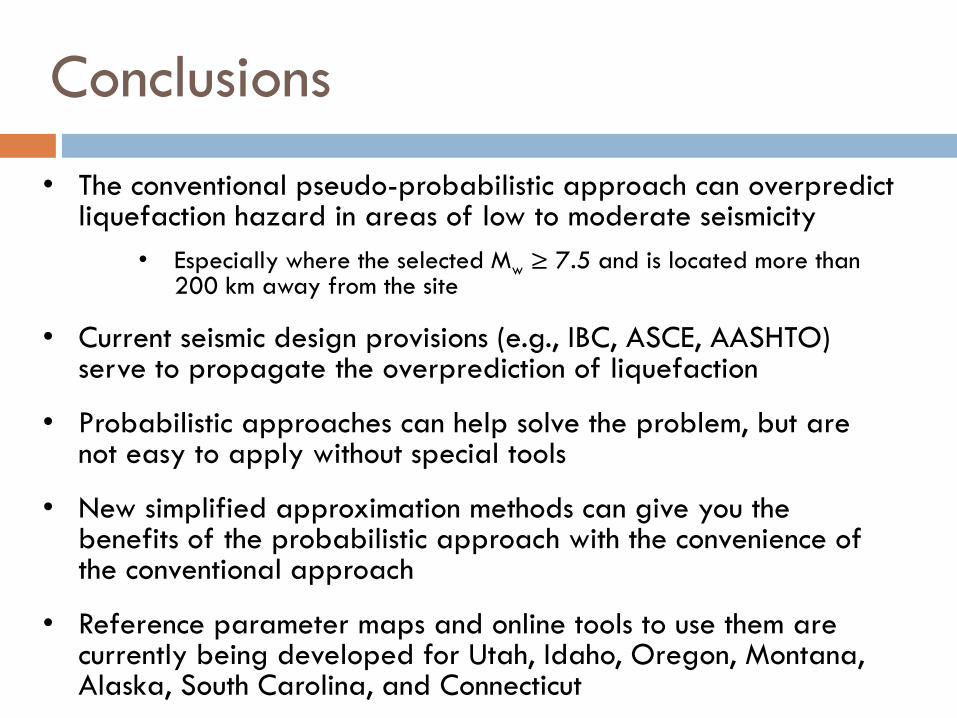
Conclusions
• The conventional pseudo-probabilistic approach can overpredictliquefaction hazard in areas of low to moderate seismicity
• Especially where the selected Mw ≥ 7.5 and is located more than 200 km away from the site
• Current seismic design provisions (e.g., IBC, ASCE, AASHTO) serve to propagate the overprediction of liquefaction
• Probabilistic approaches can help solve the problem, but are not easy to apply without special tools
• New simplified approximation methods can give you the benefits of the probabilistic approach with the convenience of the conventional approach
• Reference parameter maps and online tools to use them are currently being developed for Utah, Idaho, Oregon, Montana, Alaska, South Carolina, and Connecticut
References
• Boulanger, R.W. and Idriss, I.M. (2012). “Probabilistic standard penetration test-based liquefaction-triggering procedure.” J.
Geotech. Geoenviron. Eng. 138(10), 1185-1195.
• Franke, K.W. and Kramer, S.L. “Procedure for the empirical evaluation of lateral spread displacement hazard curves.” J. Geotech.
Geoenvir. Eng., 140(1), 110-120.
• Franke, K.W., Ulmer, K.J., Ekstrom, L.T., and Meneses, J. (2016). “Clarifying the differences between traditional liquefaction hazard
maps and performance-based liquefaction reference parameter maps.” Soil Dynamics and Earthquake Engineering, Elsevier,
90(2016), 240-249.
• Franke, K.W., Lingwall, B.N., and Youd, T.L. (2017, under review). “Overestimation of liquefaction hazard in areas of low to
moderate seismicity due to improper characterization of probabilistic seismic loading.” Submitted to Soil Dynamics and Earthquake
Engineering, Elsevier.
• Idriss, I.M. and Boulanger, R.W. (2008). Soil Liquefaction During Earthquakes, EERI Monograph MNO-12. Oakland, CA.
• Idriss, I.M. and Boulanger, R.W. Semi-Empirical Procedures for Evaluating Liquefaction Potential During Earthquakes. Soil Dynamics
and Earthquake Engineering, Elsevier, Vol. 26, 2006, pp. 1165-1177.
• Ishihara, K., & Yoshimine, M. (1992). Evaluation of settlements in sand deposits following liquefaction during earthquakes. Soils
Found., 32, 173-188.
• Kramer, S.L., and Mayfield, R.T. (2007). “Return period of soil liquefaction.” J. Geotech. Geoenviron. Eng. 133(7), 802-813.
• Mayfield, R.T., Kramer, S.L., and Huang, Y.-M. (2010). “Simplified approximation procedure for performance-based evaluation of
liquefaction potential.” J. Geotech. Geoenviron. Eng. 136(1), 140-150.
• Ulmer, K.J. and Franke, K.W. (2015). “Modified performance-based liquefaction triggering procedure using liquefaction loading
parameter maps.” J. Geotech. Geoenvir. Eng. 04015089, DOI: 10.1061/(ASCE)GT.1943-5606.0001421
• Youd, T.L., Hansen, C.M., and Bartlett, S.F. (2002). “Revised multilinear regression equations for prediction of lateral spread
displacements. J. Geotech. Geoenvir. Eng., 128(12), 1007-1017.

THE OVERPREDICTION OF
LIQUEFACTION HAZARD IN
CERTAIN AREAS OF LOW TO
MODERATE SEISMICITYDr. Kevin Franke, Ph.D., P.E., M.ASCE
Dept. of Civil and Environmental Engineering
Brigham Young University
April 20, 2017