The optimal production channel for private

labels: Too much or too little innovation?∗

Claire Chambolle†, Clémence Christin‡, Guy Meunier†.

February 2013

Abstract

We analyze the impact of the private label production channel on innova-

tion decisions on both the private label and the national brand. The retailer

may either choose a small �rm and innovate itself, or rely on the national

brand manufacturer to produce, and innovate on, both goods. The trade-o�

between the two channels is mainly a choice between too much or too little

innovation on the private label. On the one hand, when choosing the small

�rm, the retailer over-invests to increase its buyer power. This e�ect is all

the stronger that its buyer power is initially weak. On the other hand, when

the national brand manufacturer is selected, a standard hold-up e�ect leads to

under-investment. This e�ect is reinforced when the buyer power is stronger.

Besides, the choice of the brand manufacturer may create economies of scale

that spur innovation. In equilibrium, whenever the buyer power is not too high

and when some consumers have a strong preference for the national brand, the

retailer selects the brand manufacturer (resp. the small �rm) to produce the

private label, which may be detrimental to welfare as consumers can be hurt

by too little innovation on the private label.

∗We thank Eric Avenel, Eric Giraud-H�raud, Julien Troiville, Yaron Yehezkel and participants

at EARIE 2012 as well as seminar participants at the University of Rennes and the University of

Grenoble for their useful comments and references.†INRA UR1303 ALISS and Economics Department Ecole Polytechnique.‡Corresponding author. Normandie Université, UCBN, CREM-UMR CNRS 6211, 19 Rue

Claude Bloch, F-14032 Caen, France; email: clemence.christin@unicaen.fr.

1

JEL-Classi�cation: L14, L15, L42

Keywords: Private labels, vertical relations, buyer power, innovation.

2

1 Introduction

Private labels' sales have been growing since the seventies and globally have now

reached around 25% of total supermarket sales (against 15% in 2003). In Europe

their market share is particularly high in Switzerland (46%), UK (42.5%), and Ger-

many, Spain, Belgium and France with a market share around 28 − 30%. The two

leading supermarkets in the world Wal-Mart and Carrefour respectively have sold

38% and 35% of private labels in volume in 2008.1

If initially private labels were positioned as low-quality �me-too� products, their

quality has signi�cantly improved. In 2010, a survey carried out in the U.S. found

that �44% of grocery shoppers believe store brand products are of better quality

today than they were �ve years ago�.2 Private labels are also more and more in-

novative. Accordingly, the average price level in many private label categories has

increased (e.g., Connor and Peterson, 1992).

In most countries three sources of private label production generally co-exist.

First, the retailer buys the private label from small and medium �rms or directly

holds the production facilities. Second, the national brand producers themselves are

often supplying the private label to retailers. Finally, the retailer can entrust the

production of its private label to powerful manufacturers, which have specialized in

the production of private labels only and may work for several retailers at a time.3 In

France, about 70% of private labels are still produced by small �rms but a growing

share is produced by either the national brand producers or by large specialized

private label manufacturers. In the U.S., according to Quelch and Harding (1996),

more than 50% of U.S. manufacturers of branded consumer packaged goods make

private label goods as well. Some national brand manufacturers are sometimes

leaders on the private label good production. For instance, Heinz is a major supplier

of private-label baby food. Finally, large �rms specialized in the production of

private labels and which have reached a critical mass through successive merger

1Source: Planet Retail, 2008.2Survey by Mintel research, quoted in "Private Label Gets a Quality Reputation, Causing

Consumers to Change Their Buying Habits", CHICAGO, Jan. 20, 2011 /PRNewswire/.3For instance in the U.S., Richelieu Foods, a private label food manufacturing company founded

in 1862 which produces frozen pizza, salad dressing, sauces, marinades, condiments and deli salads

to be marketed by other companies as their store brand, makes more than 200 million dollars in

yearly sales.

3

waves, represent a growing part of the total private label production.4

In this paper, our purpose is to understand the main drivers of a retailer's choice

of its private label production channel but also its consequences on product innova-

tion, consumer surplus and welfare. We compare the two main production channels

only: by the national brand producer and by small �rms.5 We show that the e�ect

of the retailer's choice on the qualities of the two types of goods (national brand and

private label) depends both on the balance of power between the retailer and the

national brand manufacturer and on potential cost savings on quality investments.

The economic literature has mostly analyzed the retailer's rationale for launch-

ing private labels. The industrial organization and marketing literature has often

presented private labels as a means for retailers to better discriminate demand and

to leverage their buyer power. A direct argument is that retailers can exchange one

private label supplier for another more easily: the retailer owns the label, not the

manufacturer. Another reason outlined by Mills (1995) is that a retailer may use

a private label to increase its outside option pro�t in its bargaining towards brand

manufacturers. Finally, private labels can also be used more directly to increase

di�erentiation among stores, i.e to increase store loyalty and thus increase both the

retailer's market power and buyer power (see Bontems et al., 1999, for a survey).

Few papers, however, have analyzed the retailer's choice of production channel for

private labels. To our knowledge, only Bergès-Sennou (2006), Tarziján (2007) and

Bergès and Bouamra-Mechemache (2011) have directly analyzed this issue. Both

Bergès-Sennou (2006) and Tarziján (2007) rule out the issue of quality investments.

The former focuses on the e�ect of consumer loyalty to a store and/or a national

brand on the choice of production channel for its private label, and �nds that the

retailer prefers to entrust the national brand producer with the private label when

the bargaining power of the producer or the consumer loyalty to the national brand

is low enough. The latter analyzes how the national brand producer may have an

incentive to also produce the private label. It accounts for potential synergies a

4Krüger a private label producer of chocolate, chocolate spread and instant beverages made

1.3 billion euros of sales in 2007; Bakkavr, an Icelandic private label producer of fresh products

made 26.3 million euros of sales after a merger with the British Geest and the French 4G. See

�Concentration dans les marques d'hypers�, P.Deniel and Y. Dougin - 2007 in L'Usine Nouvelle no

3057.5We explain in section 4 why a large specialized manufacturer cannot be chosen as private label

producer in our set-up.

4

national brand manufacturer may bene�t from also manufacturing a private label

and puts them in balance with cannibalization e�ects. Indeed, when the private

label is produced by the national brand producer, its perceived quality may increase.

In contrast with these two papers, where qualities are �xed, our paper focuses on

innovation issues.

Bergès and Bouamra-Mechemache (2011) do consider quality investment issues.

However, the comparison between the two private label sources (national brand

producer or small �rms) relies mainly on an exogenous gap between the national

brand producer and the competitive fringe regarding the costs of producing the

private label. By contrast, our comparative analysis between the two alternative

private label sources relies essentially on the balance of power in the vertical channel

and an initial higher valuation granted by some of consumers to the national brand

relative to the private label. In contrast with this article, we focus on quality

investment issues for both private label and national brand products.

Our paper is also related to the literature on the role of buyer power on invest-

ment decisions within a vertical chain. On the one hand, the presence of large buyers

may induce suppliers to invest more in order to make up for their loss of bargaining

power, which eventually may raise consumer surplus and total welfare. Focusing

on technology adoption, Inderst and Wey (2003, 2007) show that buyer power may

increase suppliers' incentives to choose a technology with lower incremental cost at

higher quantities: such technology enables them to be stronger in their bargaining

with large buyers. In contrast, Battigalli et al. (2007) show that buyer power may

weaken the producer's incentive to engage in quality improvement, due to the hold-

up problem. They show under which conditions the retailers also su�er from too

low investment by the producer.

In this paper, we consider an elastic demand framework where ex ante (before

quality investments) part of consumers have a preference for the national brand

while the rest of consumers are indi�erent between the brand and the private label.

We study a game where a monopolist retailer can �rst entrust either the national

brand producer or a competitive fringe for the production of its private label. In the

following stage, innovation choices, say quality investments, are made and �nally

the retailer chooses the products to put on its shelves and sets their prices.

We analyze the impact of the choice of the private label production channel

on the innovation on both the private label and the national brand. As the buyer

5

power in the vertical chain creates hold-up on the quality investments of the national

brand producer, its innovation decisions are suboptimal. By contrast, when the

retailer invests (via a competitive fringe) in the quality of its private label, it over-

invests in order to increase its outside option in its bargaining with the national

brand producer. Besides, when the national brand producer is also the private

label producer, any quality investment increases both its national brand quality

and the private label quality. By contrast, a competitive fringe only invests to

increase the private label quality. Therefore, choosing the national brand producer

over the competitive fringe avoids a duplication of innovation costs. The balance

between these e�ects determines which type of private label production channel is

optimal depending on both the buyer power of the retailer and the level of initial

preference that some consumers grant to the national brand relative to the private

label. These e�ects explain why the retailer may alternatively prefer selecting the

brand producer or the competitive fringe to supply the private label. When the buyer

power of the retailer is low and the initial preference for the brand is large enough,

the retailer selects the brand producer as a private label supplier. This choice may

be detrimental to consumers and welfare as it may lead to less innovation on the

private label.

The article is organized as follows. Section 2 derives the model assumptions. Sec-

tion 3 analyzes the two options, a competitive fringe or the national brand producer

itself, to supply the private label. In Section 4, we determine the optimal choice of

private label production channel for the retailer according to its buyer power and the

initial brand advantage. Section 5 derives the implication for consumer surplus and

welfare. In Section 6, we provide an extension where entrusting the brand producer

with the production of the private label does not avoid the duplication of investment

costs, and show that the retailer may still want to sign entrust the brand producer

with the production of the private label. Section 8 concludes.

2 The model

We consider a framework in which a monopolist retailer, R, may sell two di�erent

goods: a national brand, B, supplied by a brand producer, P, and a private label,

L, that is produced either through a competitive fringe of small producers denoted

by f or by P itself. Only the retailer can sell goods on the �nal market.

6

Firms may innovate by investing in the quality of both B and L. Innovation in the

Consumer-Packaged-Good industries mainly consists in ensuring constant quality

improvements and radical innovations are rare events (Pauwels and Srinivasan, 2004;

Steiner, 2004).6 We thus focus in this model on deterministic quality investments.

P can make a quality investment at a cost C(kB) in order to increase the quality of

B by kB, and hence, increase the utility that the consumer gets from its consumption.

Similarly, when R buys its private label from a competitive fringe, we assume that R

invests in the quality kL of its private label and supports the associated cost C(kL).

Indeed, because of perfect competition in the fringe, R captures the joint pro�t if

supplied by a fringe �rm, and therefore everything happens as if it were vertically

integrated with the private label manufacturer. By contrast, when R entrusts the

production of its private label to the producer P, P chooses both investment levels kB

and kL and the associated cost, entirely borne by the producer, is C(Max[kB, kL]).

Indeed, we assume here that for a given level of quality investment there is no

additional cost to o�er two goods instead of one: the �rm can di�erentiate the

private label from the national brand at no cost. The di�erence is only a matter

of packaging and the associated packaging cost is neglected. Therefore, if kB > kL

(respectively kL > kB) the producer has to pay the cost C(kB) (resp. C(kL)) and can

o�er the other product at any downgraded level of quality kL < kB (resp. kB < kL)

without additional cost. Investment costs are quadratic and identical for all �rms

and products: C(ki) =k2i2where i = B,L. We assume that investment costs are

the only costs borne by the producers: the marginal cost of production is assumed

constant and normalized to 0.

Consumers are heterogeneous in their tastes. The total mass of consumers is

normalized to 1. A share λ of the population are �brand lovers� who, absent any

di�erence in quality investments and prices, have a strict preference for good B. The

remaining fraction (1− λ) of consumers are �standard consumers� who, absent any

di�erence in quality investments and prices, have exactly the same demand for B

and L.

Given the prices pB for the national brand and pL for the private label, the

surplus of a brand lover is:

Sδ = (v + δ + kB)qB + (v + kL)qL −(qB + qL)2

2− pBqB − pLqL (1)

6Radical innovations represent about 6% of total innovation output (Martos-Partal, 2012).

7

if it purchases a quantity qi of good i (i = B,L), while a standard consumer then

earns a surplus:

S0 = (v + kB)qB + (v + kL)qL −(qB + qL)2

2− pBqB − pLqL. (2)

The total consumer surplus is then S = λSδ + (1 − λ)S0. The demand for the

national brand is as follows:

• If pL < v + kL, then the two goods can be sold and we have:

DB =

v + λδ + kB − pB if pB ∈ [0, kB − kL + pL],

λ(v + kB + δ − pB) if pB ∈ [kB − kL + pL, pL + δ + kB − kL],

0 if pB > pL + δ + kB − kL,

and demand for the private label is given by:

DL =

0 if pB ∈ [0, kB − kL + pL],

(1− λ)(v + kL − pL) if pB ∈ [kB − kL + pL, pL + δ + kB − kL],

v + kL − pL if pB > pL + δ + kB − kL,

• If, however, pL ≥ v + kL, then DL = 0, and again we have three cases:

DB =

v + λδ + kB − pB if pB ∈ [0, v + kB],

λ(v + kB + δ − pB) if pB ∈ [v + kB, v + δ + kB],

0 if pB > v + δ + kB,

This demand speci�cation, initially introduced by Soberman and Parker (2004),

is sustained by a survey conducted in the U.S. in 2010, that showed that 19% of

consumers believe that it is worth paying more for name brand products.7 We

assume that δ < v: even if all consumers were �brand lovers�, selling the national

brand cannot double the market size.

The timing of the game is as follows:

1. Choice of the private label channel

R may sign a contract with P that associates a transfer Y (positive or negative)

for the delegation of the production of L. This case is named �Channel P� and

denoted by a superscript P .

7Survey by Mintel Research. See footnote 2.

8

Otherwise, a �rm from the competitive fringe produces L. This case is named

�Channel f� and denoted by a superscript f .

We assume that the quality of the private label is not contractible.

2. Innovation

• Channel P: P chooses both qualities kL and kB, and bears the associated

cost C(Max[kL, kB]).

• Channel f: P invests kB in good B at a cost C(kB) and simultaneously,

R invests kL in good L at a cost C(kL).

Firms can no longer invest in quality after the end of this innovation stage.8

3. Bargaining

• Channel P: R and P bargain over a �xed transfer for the delivery of both

B and L to the retailer. The producer has no outside option, whereas

the retailer can still sell a private label of quality kL = 0 (no investment

could be done).

• Channel f: R and P bargain over a �xed transfer for the delivery of B.

The producer has no outside option, the retailer can still sell a private

label of quality kL.

4. Sales R sells either one or the two goods to consumers and sets the retail

prices pL and pB.

We consider subgame perfect equilibrium and proceed by backward induction.

As the last stage is not a�ected by the production channel choice, we solve it

here. Qualities kB and kL are �xed and R chooses the prices that maximize the

industry pro�t. Three cases may arise: �rst R may sell only L to all consumers;

second R may sell the two goods B and L and thus discriminate between brand

lovers and others; �nally, R may sell only B to all consumers.

8It should be noted that, in contrast with Bergès and Bouamra-Mechemache (2011) where

the retailer always has control over the quality of the private label, regardless of the production

channel, we assume here that the private label quality is not contractible and can, thus, be freely

chosen by the private label supplier.

9

- When only the private label is sold, the industry pro�t is (v+ kL− pL)pL, and

R sets the optimal price pL = v+kL2

.

- When both the private label and the national brand are sold, the industry

pro�t is λ(v+ δ+kB− pB)pB + (1−λ)(v+kL− pL)pL, and R sets the optimal

prices pL = v+kL2

and pB = v+δ+kB2

.

- When only the brand is sold, the industry pro�t is (v + λδ + kB − pB)pB, and

R sets the optimal price pB = v+λδ+kB2

Which option is the most pro�table depends on the two qualities, and the

monopoly pro�t, denoted π(kL, kB), is as follows:

π(kL, kB) =

14(v + kL)2 for kB ∈ [0, kL − δ],λ4(v + δ + kB)2 + 1−λ

4(v + kL)2 for kB ∈ (kL − δ,

√(kL + v)2 + λδ2 − v],

14(v + λδ + kB)2 for kB >

√(kL + v)2 + λδ2 − v.

(3)

For given quality levels, the industry pro�t is independent of whether the private

label is produced by a competitive fringe or by the brand manufacturer. Given our

assumption δ < v, when R sells only the national brand, it strictly prefers to sell B

at a lower price to all consumers rather than sell it at a higher price to brand lovers

only.

In Stage 3, we adopt a standard Nash bargaining approach to model the nego-

tiation between R and P. The exogenous bargaining power of R relative to P is a

parameter α ∈ [0, 1]. In equilibrium, R (respectively P) earns its outside option

pro�t plus a share α (resp. 1− α) of its incremental gain from trade with P. Since

the national brand producer cannot supply its products to any other �rm than the

retailer, its outside option in all subgames is always 0. On the contrary, in case of

a failure in the bargaining with P, the retailer can always turn to the competitive

fringe and sell only the private label on the �nal market. The outside option pro�t

of R is then denoted by π̄ = 14(v + kL)2, with kL the quality of the private label

produced by the competitive fringe.

3 Private label production channel and innovation

In this section, we solve Stages 2 and 3 of the game in order to highlight how

the choice of the private label production channel a�ects the innovation on both

10

the national brand and the private label. We �rst solve the subgame �Channel P�

in which P produces the private label and is the only �rm that invests in quality

improvements. Then, we solve the subgame �Channel f�, in which a competitive

fringe produces L and both P and R invest in quality.

3.1 Channel P

In this subsection, R entrusts P for the production of the private label, and P

thus chooses both qualities kL and kB and pays the associated investment cost

C(Max[kB, kL]). In stage 4, the joint pro�t of the industry is given by π(kL, kB)

de�ned by (3).

At the bargaining stage, the sharing of the pro�t π(kL, kB) between the producer

and the retailer depends on the relative bargaining power of each �rm, given by α

(resp. 1− α) and their outside options. P has no outside option pro�t whereas the

outside option pro�t of R comes from the sale of a private label without any quality

upgrading. Indeed, by choosing Channel P, R committed itself not to invest in the

quality of the private label, and in stage 3 it is too late for R to innovate. In case of

a disagreement with P in the bargaining stage, R could therefore still sell a private

label produced by a competitive fringe, but with quality kL = 0. As a consequence,

its outside option is π(0) = v2/4. The Nash bargaining leads to the following pro�ts:

ΠPP (kL, kB) = (1− α) [π(kL, kB)− π(0)]− C(Max[kB, kL]) (4)

ΠPR(kL, kB) = π(0) + α [π(kL, kB)− π(0)] (5)

Lemma 1. For any quality investment k, the qualities maximizing π(kL, kB) subject

to kB, kL ≤ k are kL = kB = k.

Proof. See Appendix A.1.

Whatever the investment made by the producer it is always optimal for P, as

well as for the total industry pro�ts, to sell both goods at similar quality; P has no

incentive to downgrade the quality of one of the goods. Then, the total industry

pro�t net of investment cost is

ΠP (kL, kB) = π(kL, kB)− C(Max[kB, kL]). (6)

with kB = kL = k. The quality maximizing the net industry pro�t ΠP (k, k) is

v+λδ and we denote by ΠP∗ the corresponding maximum total industry pro�t with

11

Channel P. We will henceforth refer to this quality level as the �optimal� quality, in

the sense that it is optimal from the point of view of the vertical structure.

The equilibrium quality investment of the producer, however, is determined by its

marginal bene�t (1−α) [∂π/∂kB + ∂π/∂kL]: the equilibrium quality is thus strictly

lower than the optimal quality. Given that the producer has to share the marginal

bene�t of its investment with the retailer, it always underinvests in quality. This

so-called �hold-up e�ect� is increasing with the bargaining power of the retailer α.

Proposition 1. There exists a unique equilibrium of the subgame Channel P.

In this equilibrium P chooses the same quality for both B and L,

kPB = kPL = (v + λδ)1− α1 + α

,

and both goods are sold to consumers.

Proof. See Appendix A.2.

Because of the hold-up e�ect, the producer under-invests relative to the optimal

quality: kP < δλ + v. Replacing kP in eq. (6), the corresponding total industry

pro�t obtained with channel P is denoted ΠP and the di�erence ΠP − ΠP∗ ≤ 0 is

only due to the hold-up ine�ciency. The di�erence is brought to 0 when α = 0

because then, all the power is in the hands of P and there is no more hold-up.

3.2 Channel f

In this subsection, R entrusts a �rm from a competitive fringe with the production

of its private label. P (resp. R) thus chooses quality kB (resp. kL) and pays the

associated investment cost C(kB) (resp. C(kL). In the bargaining stage, the total

pro�t from sales π(kL, kB) is shared among the two �rms. The outside option pro�t

of the retailer amounts to the pro�t it would earn if it sold only its private label

to all consumers, π(kL) = 14(v + kL)2. By contrast, P has no outside option pro�t.

Accordingly the pro�ts are:

ΠfP (kL, kB) = (1− α) [π(kL, kB)− π(kL)]− C(kB) (7)

ΠfR(kL, kB) = π(kL) + α [π(kL, kB)− π(kL)]− C(kL) (8)

An equilibrium of Channel f is completely characterized by a couple of qualities

chosen by �rms. Indeed, it corresponds to a Nash equilibrium of the game with

12

pro�ts given by (7) and (8). In the last stage three cases may arise: either both

goods are sold or only one of them. Depending on the values of the parameters α, δ,

and λ, we will show that all three situations may arise along an equilibrium path and

that one, two or three equilibria may co-exist. We proceed by �rst considering three

equilibrium candidates de�ned by their couples of qualities and then determining

under which conditions each candidate is indeed an equilibrium. Furthermore, in

case of co-existence there is always an equilibrium that Pareto dominates the others

and we consider that it will be played. Consequently, the equilibrium qualities of

the subgame Channel f can be denoted kfB, kfL without ambiguity.

Lemma 2. There are three possible types of equilibrium of the subgame Channel f :

(kfL, kfB) =

(kBLL , kBLB ) = (v 1−αλ

1+αλ, λ(1−α)(v+δ)

2−λ(1−α) ) if both B and L are sold,

(kLL, kLB) = (v, 0) if only L is sold,

(kBL , kBB) = (v 1−α

1+α, (1−α)(v+λδ)

1+α) if only B is sold.

Note that in the coexistence equilibrium, both kBLB and kBLL are strictly decreas-

ing in the retailer's buyer power. The fact that kBLB decreases in α is not surprising

as it directly comes from the hold-up e�ect. More interestingly, the quality of the

private label kBLL also decreases in α. Indeed, R obtains its buyer power from two

sources: �rst its exogenous buyer power parameter, α, and second its outside option

pro�t π. When α is low, the retailer's buyer power is mainly driven by its outside

option pro�t, and the retailer thus has a greater incentive to raise it by increasing

kL.

The domain of existence of each type of equilibrium is now determined by check-

ing the incentives of P and R to shift from one case to the other. Note that whenever

there is a multiplicity of equilibria, there is always one which Pareto dominates the

others. We assume henceforth that, in case of coexistence, the dominant equilibrium

is played. Appendix A.4 gives the complete proof.

Proposition 2. In the subgame Channel f, if λ <√17−32

:

- there exists a dominant equilibrium, denoted BL, where both the national brand

and the private label are sold if:

δ > δ1 = vmax

{2− (1− α)λ√

1 + αλ− 1,

√2(2− (1− α)λ)

1 + αλ− 1

}

13

- Otherwise, the unique equilibrium, denoted L, is such that only the private

label is sold.

When λ ≥√17−32

:

- If α < 2λ − 1 and δ ∈ [δ3, δ4], there exists a dominant equilibrium, denoted

(B), such that only the brand is sold.

- Otherwise, if δ > δ1 the dominant equilibrium is BL and if δ ≤ δ1, the unique

equilibrium is L.

Proof. See Appendix A.4 for the full proof and the expressions of thresholds δ3 and

δ4.

In Proposition 2, the parameter δ is used to characterize the frontiers between

the three types of equilibria.

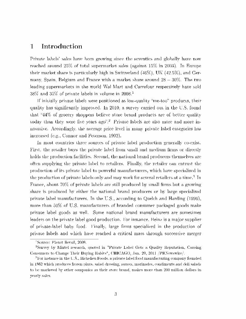
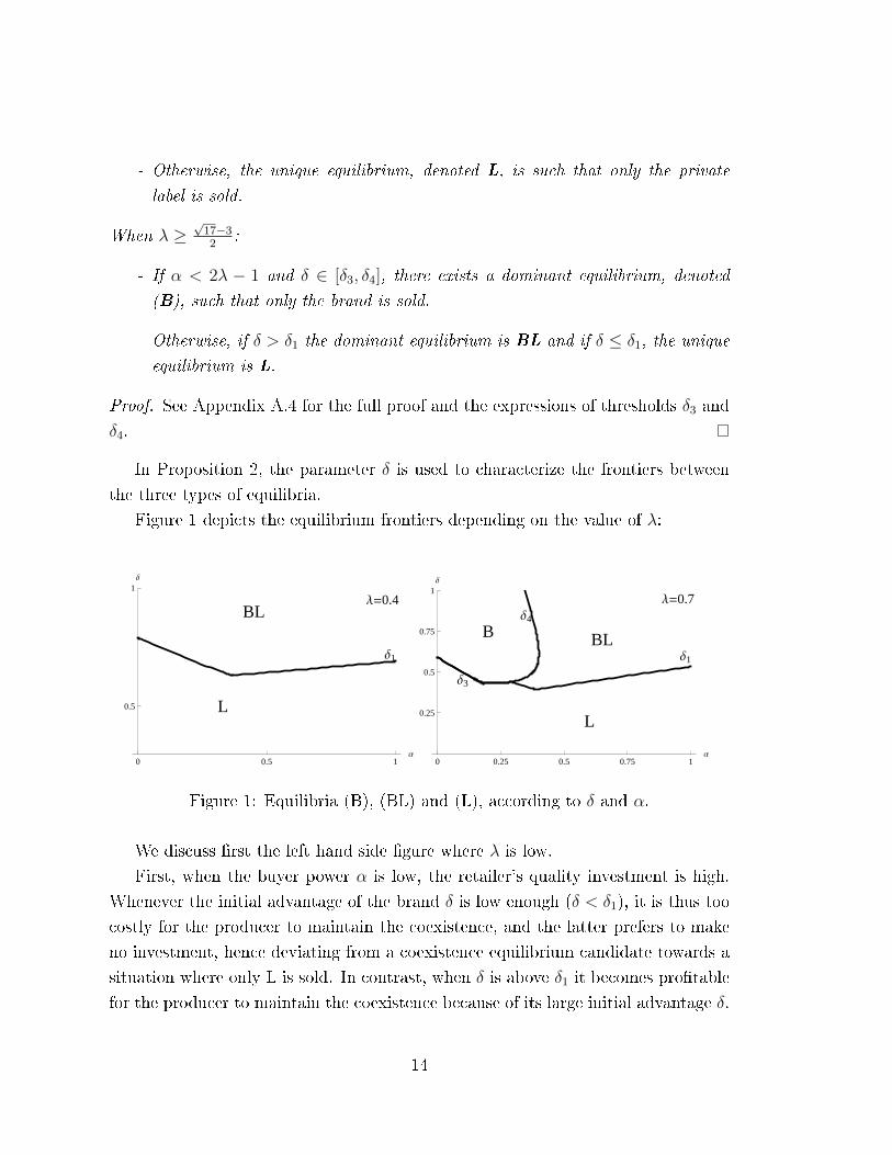
Figure 1 depicts the equilibrium frontiers depending on the value of λ:

0 0.5 1Α

0.5

1∆

BL

L

∆1

Λ=0.4

0 0.25 0.5 0.75 1Α

0.25

0.5

0.75

1∆

L

BLB∆1

∆3

∆4

Λ=0.7

Figure 1: Equilibria (B), (BL) and (L), according to δ and α.

We discuss �rst the left hand side �gure where λ is low.

First, when the buyer power α is low, the retailer's quality investment is high.

Whenever the initial advantage of the brand δ is low enough (δ < δ1), it is thus too

costly for the producer to maintain the coexistence, and the latter prefers to make

no investment, hence deviating from a coexistence equilibrium candidate towards a

situation where only L is sold. In contrast, when δ is above δ1 it becomes pro�table

for the producer to maintain the coexistence because of its large initial advantage δ.

14

Second, for high values of buyer power, the quality investment of P is low. When-

ever the initial advantage of the brand δ is low enough the retailer has no incentive

to discriminate by selling the brand, and instead prefers to sell a better quality pri-

vate label to all consumers. When δ is high enough, however, the retailer �nds it

more pro�table to sell both B and L to discriminate consumers rather than selling

only L.

We now discuss the right hand side �gure where the equilibrium B exists. Note

that B arises when λ is high since more consumers are ready to pay for the brand.

Then, B is favored by a high value of δ and low buyer power α. As mentioned above,

the lower the buyer power, the higher the retailer's quality investment. This may

still discourage coexistence, but here, when δ is high enough, it is more pro�table

to give up on the private label rather than the brand.

The total industry pro�t (net of R&D costs) is:

Πf (kL, kB) = π(kL, kB)− C(kB)− C(kL). (9)

We determine the optimal brand and private label qualities, that is the qualities that

would maximize the net industry pro�t given by (9) and we denote the corresponding

industry pro�t by Πf∗. As in the previous case, �rms do not choose these optimal

quality investments. There are two types of distortions at stake.

When the producer invests (in B and BL) there is a hold-up e�ect, similar to the

e�ect at play in the subgame Channel P: P's investment is determined by its own

marginal bene�t, (1−α)∂π/∂kB, instead of being determine by the marginal bene�t

of the industry, ∂π/∂kB. In addition to this, another extreme form of hold-up e�ect

can arise in Channel f because of the retailer's outside option. Even though the

marginal bene�t of the producer's investment, and thus the value of kB, does not

depend on π, the producer's incentive to invest at all is in�uenced by the outside

option of the retailer. If the retailer's quality kL is too high, then π(kL) is too high

for the producer to earn a positive pro�t from selling its good, and P may therefore

decide to neither invest nor supply the brand. In this case, only the private label is

sold.

The outside option of the retailer plays an opposite role on the retailer itself.

Indeed, in order to increase its outside option, and therefore its bargaining power

vis-à-vis the producer, the retailer tends to over-invest in quality. This only a�ects

cases where the producer indeed earns a share of the pro�t, that is when both goods

15

or only the national brand is sold. In these two cases, the quality of the private

label that would maximize the net industry pro�t would be respectively v(1−λ)1+λ

and

0, and the quality choice of R is higher than these optimal quality levels due to this

"over-investment e�ect". The "over-investment e�ect" decreases with the bargaining

power of the retailer α.

To summarize, the di�erence between Πf and Πf∗ results from both a hold-up

e�ect on the brand quality, which increases in α, and an over-investment e�ect on

the private label quality, which decreases in α.

4 Choice of the private label production channel

In stage 1, R chooses the production channel that leads to the highest total industry

pro�t. Indeed, as long as total industry pro�t is higher in a given Channel, in stage

1 P and R can always �nd a transfer Y such that both P and R are each strictly

better o� than if R chose the other channel. Therefore, R chooses channel P if

total industry pro�t in the subgame �channel P� is larger than total industry pro�t

in the subgame �Channel f�. More formally, R chooses Channel P if and only if

∆P,fdef= ΠP − Πf > 0. Henceforth, we will simply refer to �Channel X� as the

subgame in which Channel X is chosen by the retailer.

There are several e�ects at stake that explain whether one option is preferred to

the other. Note that if it were possible for the two �rms to write complete contracts,

then the best option would always be to make P supply both B and L because it

would prevent a costly replication of investments in qualities (ΠP∗ > Πf∗) However,

contracts are incomplete and quality investments are not contractible. This induces

ine�ciencies in both Channels that could explain why the retailer may want to

manufacture its private label through a competitive fringe. One way to disentangle

these e�ects is to write the comparison:

∆P,f =[ΠP∗ − Πf∗]︸ ︷︷ ︸cost duplication

+[ΠP − ΠP∗]︸ ︷︷ ︸

hold-up in Channel P

+[Πf∗ − Πf

]︸ ︷︷ ︸hold-up and over-investment

in Channel f

(10)

The �rst term casts the positive e�ect related to the absence of cost duplication in

Channel P. It is the di�erence between the optimal industry pro�ts without cost

duplication and with duplication. The second term is negative and corresponds to

16

the loss resulting from the hold-up e�ect in Channel P. This term is equal to 0 for

α = 0 and increases with respect to the bargaining power of the retailer. Finally,

the third term is positive and encompasses the gain in Channel f when correcting

both for the hold-up and the over-investment e�ects described in subsection 7.1.

The precise characteristics of this last term depend upon the type of equilibrium in

Channel f.

The following proposition establishes the conditions under which R chooses

Channel P in stage 1.

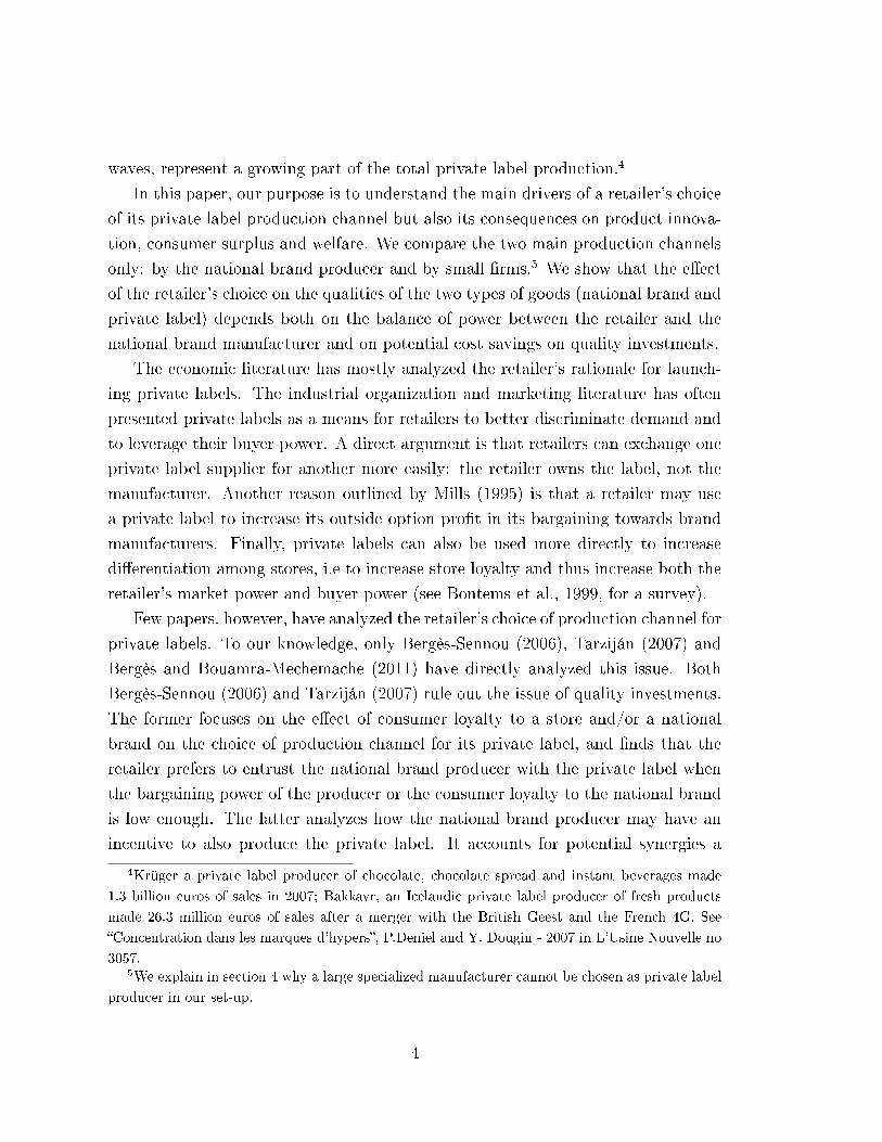
Proposition 3. There exist two thresholds δ∗ and δ∗∗ such that whenever δ∗ < δ <

δ1 or δ > max{δ1, δ∗∗}, R chooses Channel P.

Proof. See Appendix.

In �gure 3, we draw the thresholds mentioned in Proposition 3 together with

the frontier between the equilibria (L) and (BL) highlighted in 7.1, for λ = 0.4 and

v = 1.

0 0.5 1Α

0.5

1∆

OBLSign with P

OL

∆2

∆1

∆*

∆**

Figure 2: Equilibrium of the game as a function of α and δ.

Consider �rst the case where the equilibrium of Channel f is to sell the two goods

(BL). As explained above by eq. (10), switching instead to Channel P has three

di�erent e�ects on quality decisions. First, it avoids the duplication of investment

costs which tends to increase the qualities of the two goods. Second, it creates a

hold-up e�ect on the quality investment of the private label. Indeed, the producer

now invests in the quality for the private label, and has to share the gains of this

17

investment with the retailer. This second e�ect tends to lower the quality of the

private label. Finally, it destroys the incentive of R to over-invest in the private

label quality. Although this last e�ect also reduces kL, it brings it closer to the

joint-pro�t maximizing quality.

As a result of these three e�ects, when the equilibrium in Channel f is (BL), if the

retailer chooses Channel P the quality of the national brand always increases while

the e�ect on the quality of the private label is ambiguous. The following lemma

summarizes the results.

Lemma 3. If λ >1+α−√

1+α(2+(9−8α)α)2(−1+α)α , there exists a threshold δ̂ = 2αv(1−λ)

(1−α)λ(1+αλ) > 0

such that whenever δ > δ̂, we have kPL > kfL. Otherwise, we have kPL < kfL.

Therefore, a situation where the retailer chooses Channel f may, despite the

duplication of quality investment costs, increase the joint pro�t of P and R. The

bene�t of selecting Channel f increases when α is large and δ is low. Indeed, as the

bargaining power of the retailer increases, the over-investment problem is reduced,

which mitigates the third e�ect, whereas the hold-up problem becomes stronger,

which increases the second e�ect. The �rst e�ect is all the stronger that δ is large,

as the joint-pro�t of the industry then increases more with the quality of the national

brand.

Consider now the case where the equilibrium in Channel f is to sell only the

private label (L). We obtain the following corollary:

Corollary 1. Whenever δ∗ < δ < δ1, selecting Channel P is the only way to main-

tain the brand on the retailer's shelves.

In Channel P, as the investment in quality is common to the two goods, the

producer never has an incentive to invest 0 on the national brand. The opportunity

for P to also produce L enables the industry to maintain the diversity of the products

o�ered to consumers. When δ < δ1, by investing itself in the private label quality,

the retailer would indeed over-invest and thus discourage any investment and sale

of the brand. Another reason why supplying the private label together with the

national brand may allow the producer to maintain its product on the shelves is

that the retailer's outside option when both goods are sold is lower in Channel P.

Therefore, for any given value of kB, there are more cases where the producer can

earn a pro�t by selling the national brand. Because of the hold-up e�ect, however,

18

it is still possible that the retailer will sign with a fringe to produce its private label.

Again, the bene�t of entrusting the production of the private label to P is then

increasing in δ and decreasing in α.

Corollary 2. When an equilibrium (B) exists in Channel f, selecting Channel P is

the only way to maintain the private label on the retailer's shelves.

The insight of the above corollary is as follows. When the equilibrium (B) exists,

the industry pro�t in Channel f is maximized through the sale of only one good B to

all consumers, but, in equilibrium (B), R has to sell B at the same price to all con-

sumers. Now, by choosing Channel P, the same good can be sold at di�erent prices

and under di�erent packages to the two types of consumers. Therefore, choosing

Channel P enables to discriminate among consumers and thus raises the joint pro�t

of the industry. Another ine�ciency disappears when R chooses Channel P. Indeed,

when (B) is an equilibrium, R spends C(kBL ) > 0 to raise its share of the joint pro�t

but this investment has no e�ect on the joint industry pro�t. When P supplies the

private label, R no longer invests and therefore avoids an ine�cient duplication of

investment costs.

This case also illustrates the cannibalization of sales, a drawback often brought

forward in the debate on whether the national brand producer should start making

private labels (See Quelch and Harding, 1996): The brand loses market shares to

the bene�t of the private label.

Finally, note that in this framework, entrusting a powerful specialized private

label manufacturer would combine both the hold-up and the cost duplication inef-

�ciencies and would thus never arise in equilibrium.9

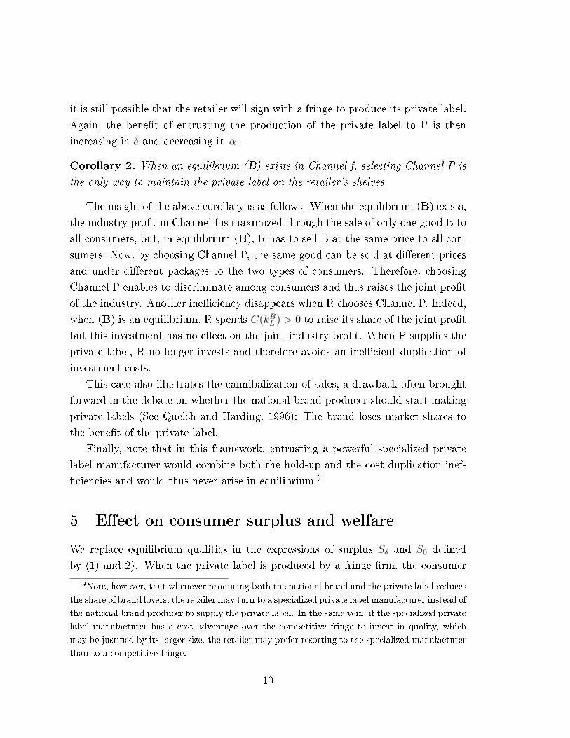
5 E�ect on consumer surplus and welfare

We replace equilibrium qualities in the expressions of surplus Sδ and S0 de�ned

by (1) and 2). When the private label is produced by a fringe �rm, the consumer

9Note, however, that whenever producing both the national brand and the private label reduces

the share of brand lovers, the retailer may turn to a specialized private label manufacturer instead of

the national brand producer to supply the private label. In the same vein, if the specialized private

label manufacturer has a cost advantage over the competitive fringe to invest in quality, which

may be justi�ed by its larger size, the retailer may prefer resorting to the specialized manufacturer

than to a competitive fringe.

19

surplus is :

Sf =

v2

2if only L is sold.

λ (v+δ)2

2(2−(1−α)λ)2 + (1− λ) v2

2(1+αλ)2if B and L are sold.

(v+δλ)2

2(1+α)2if only B is sold.

When the private label is produced by P, the consumer surplus is given by:

SP = λ[2v + (1− α)δλ+ (1 + α)δ]2

8(1 + α)2+ (1− λ)

[2v + (1− α)λδ]2

8(1 + α)2.

In equilibrium, R chooses Channel P whenever this strategy raises the joint

pro�t of the industry relative to the alternative choice of Channel f. The e�ect on

consumer surplus may, however, be ambiguous.

First, note that in all cases R sets the monopoly prices on the retail market.

As a consequence, only two factors may a�ect the consumer surplus: the quality of

the products sold and the ability of the retailer to discriminate or not among brand

lovers and standards consumers. By comparing consumer surplus, we obtain the

following proposition.

Proposition 4. When in equilibrium R chooses Channel P, it may hurt consumer

surplus for two main reasons:

- When the resulting decrease in the quality of the private label L is too large

relative to the increase in the quality of the national brand B.

- When choosing Channel P enables R to discriminate among consumers instead

of selling B at the same price to all consumers.

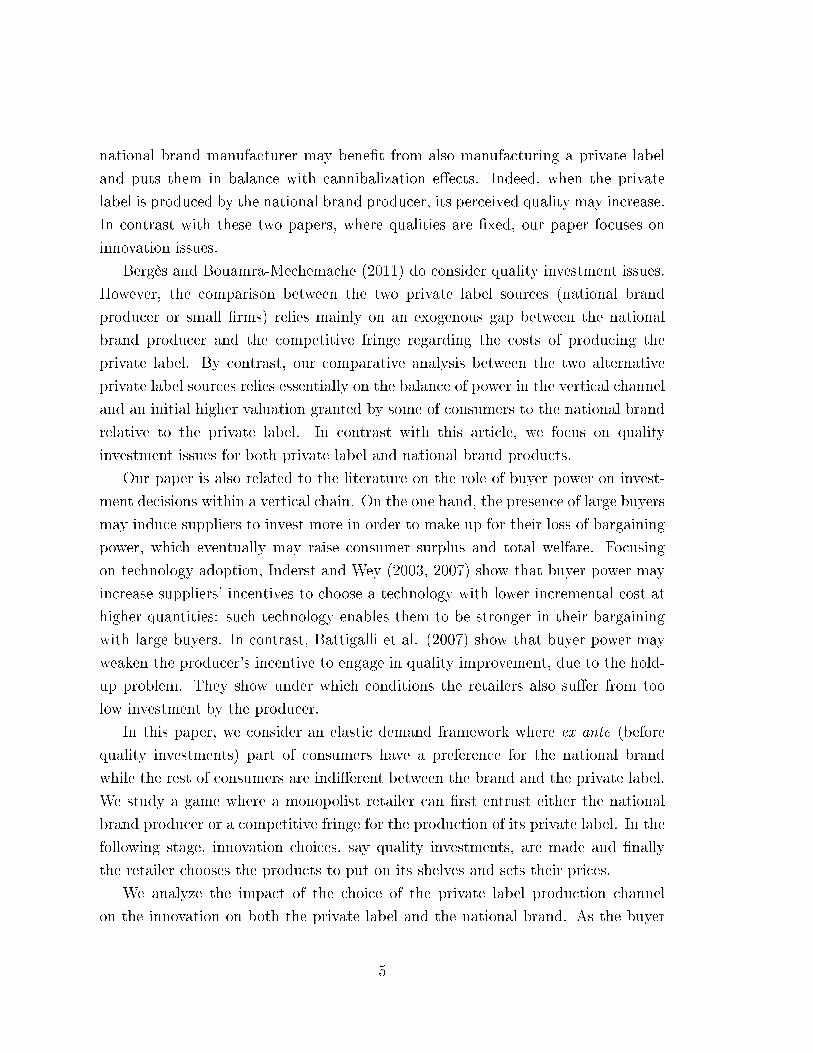
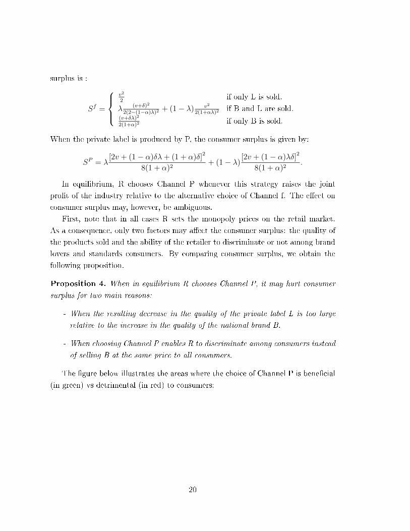
The �gure below illustrates the areas where the choice of Channel P is bene�cial

(in green) vs detrimental (in red) to consumers:

20

0 0.25 0.5 0.75 1Α

0.25

0.5

0.75

1∆

L

BLContract

with P

Figure 3: E�ect on consumer surplus for λ > λ.

The red area in the North-West is the negative e�ect of discrimination on con-

sumer surplus.This e�ect arises only when, provided Channel f is chosen, (B) is an

equilibrium. In particular, when λ < λ this negative e�ect on consumer surplus

never appears. In the other distinct red area, it is the negative e�ect of the lowering

in the quality of L which explains the negative e�ect on the consumer surplus. This

e�ect appears when α is large enough because the hold-up e�ect remains important

when R chooses Channel P, and thus the quality investment on L is much lowered,

while the increase in the quality investment on B is not so large.

Proposition 5. When in equilibrium R chooses Channel f, it is always bene�cial

both for industry pro�t and social welfare.

Indeed, if R chooses Channel f, it means that the positive e�ect of avoiding both

a duplication of investment costs and the over-investment e�ect is not su�cient to

compensate the lowering in the quality of L due to the hold-up e�ect. A fortiori

in that case, choosing Channel f bene�ts consumers even more, as they are a�ected

only by the quality investments and not by the form of the costs (with or without

duplication). Therefore, consumers and industry interests are always aligned.

21

6 Cost duplication and choice of the private label

production channel

In the previous section, we have shown that selecting Channel P, despite the bene�t

of avoiding a duplication of costs, was not always optimal for the industry because of

strategic e�ects on quality improvements. In this section, we assume that choosing

Channel P now implies the same duplication of investment costs as choosing Channel

f: P has to pay two separate costs to invest in the quality of the brand and in the

quality of the private label it he intends to sell both goods. Interestingly, we now

show that although one of the main bene�t of choosing channel P, i.e to avoid the

duplication of costs, has been withdrawn, the retailer may still select Channel P

only as a result of the balance of opposite strategic e�ects on quality improvements.

The full resolution of this case is given in Appendix (??). We brie�y discuss the

e�ects at play in what follows.

Proposition 6. Entrusting the national brand producer with the production of the

private label may be pro�table for the industry even with investments cost duplication.

Channel f is unchanged, so qualities, prices and quantities sold are exactly the

same as in the previous case. The equilibrium in this subgame is given by Proposi-

tions 2 and ??.

Channel P is modi�ed by the duplication of cost. The national brand producer

now has to pay an investment cost C(kB) to increase the quality of the national

brand by kB, and an additional investment cost C(kL) to simultaneously increase the

quality of the private label by kL. The total pro�t of the industry is therefore denoted

Π̃P (kL, kB) and is identical to the total industry pro�t in Channel f Πf (kL, kB).

Therefore the maximum pro�t in each case is the same and Π̃P∗ = Πf∗. In Channel

P, the producer chooses both qualities and both are still sub-optimal because of the

hold-up e�ect. The resulting total industry pro�t is denoted Π̃P and we obtain the

simpli�ed comparison of the two production channels where only strategic e�ects

are at stake:

∆P,f =[Πf∗ − Πf

]︸ ︷︷ ︸hold-up and over-investment

in Channel f

−[Π̃P∗ − Π̃P

]︸ ︷︷ ︸

hold-up in Channel P

(11)

In Channel P either both B and L are sold or only B. To keep the insight simple,

we consider a case in which both goods are sold in both Channel f and Channel

22

P.10 In this case, the quality of the national brand is independent of the choice

of production channel : kfB = kPB . Indeed, for P, both the marginal bene�ts and

marginal costs associated with kB are the same in both channels. On the contrary,

the quality of the private label depends on the production channel, although it is

suboptimal in both cases. With Channel f the quality kfL is too high because of the

over-investment e�ect and with Channel P it is too low because of the hold-up e�ect.

The comparison of the two Channels is a comparison between these two sub-optimal

situations, but a simple insight can be given through the comparative statics in α.

When α = 0, that is when the bargaining power is completely in the hands of

the producer, it is clear that the hold-up e�ect in both Channel P and Channel f

disappears. The second term in eq. (11) is thus equal to 0. By contrast, the �rst

term is strictly positive since the over-investment distortion remains, and therefore,

R selects Channel P.

When α = 1, it is clear that, on the contrary, the over-investment distortion

disappears. Moreover, the hold-up e�ect on the brand is the same in both Channel

f and Channel P cases (i.e. kfB = kPB). However, an additional hold-up e�ect on the

private label arises only in Channel P. The second term in eq. (11) is thus strictly

higher than the �rst term, and Channel f is always preferred to Channel P.

By continuity, R chooses Channel P in equilibrium as long as α is small enough,

and chooses Channel f otherwise. Consumers, however, are always better o� with

Channel f, because of the higher quality of the private label in that case.11

10We prove in Appendix 6 that the situation where the two goods B and L are sold may indeed

arise in equilibrium when Channel P is chosen. Note that, due to the duplication of cost, the case

where only B is sold often appears in equilibrium. However, if only one good is sold in Channel

f or Channel P, the same kind of arbitrage arises. To entrust P for the production of the private

label is a way to prevent the retailer from in�ating the quality of the private label to increase its

share of the pie.11If only B is sold in Channel P, then consumers are better of with Channel P for low value of

α.

23

7 Managerial Implications

7.1 Individual pro�tability

Given that transfers are possible in stage 1, P and R can always �nd a mutually

bene�cial agreement to share a higher industry pro�t. Absent such transfers, the

private pro�tability of each alternative would now matter. We examine here if,

absent any transfer in stage 1, choosing channel P instead of Channel f can be

privately pro�table for the producer and the retailer.

Corollary 3. Regardless of the equilibrium market structure in Channel f, a switch

to Channel P is always pro�table for the producer.

The brand producer is always better o� in manufacturing both goods rather than

only producing its own brand. For any quality investment the comparison of the

two channels unambiguously favors Channel P: the producer's investment generates

more direct revenue and he su�ers less from the opportunism of the retailer. Even

though the industry gross revenue might be larger in Channel f than in Channel P,

thanks to a larger PL quality, the gains from trade are lower, and, hence, so is the

pro�t of the producer.

Focusing now on the retailer, two di�erent cases are worth distinguishing, de-

pending on whether the private label is sold or not in Channel f.

Corollary 4. When only the national brand is sold in Channel f, switching to Chan-

nel P decreases the pro�t of the retailer

When only the national brand is sold in Channel f, switching to Channel P

unambiguously increases total revenue. However, the brand is the only good sold in

Channel f when brand lovers are overrepresented (i.e. λ large), and the bargaining

power of the retailer is low. The former limits the gain from discrimination. The

latter implies that the possibility to strategically choose its outside option is all the

more valuable. Taken as a whole, the retailer always loses pro�ts when the structure

switches from a situation where only the brand is sold in Channel f to a situation

where both goods are sold in Channel P.

Corollary 5. When the private label is sold in Channel f (with or without the

national brand), switching to Channel P has an ambiguous e�ect on the retailer's

24

pro�t. The retailer may have a higher pro�t in switching to channel P when λ and

δ are high enough and α is intermediate.

When the private label is sold, the comparison between the two options depends

on parameters values. Even though the retailer loses its ability to strategically

manipulate its outside option he might bene�ts from switching to Channel P because

of the induced increase of industry revenue.

The trade-o�s at stake could be described by considering a change of the retailer's

bargaining power. When α increases there are two opposite e�ects on the retailer's

comparison between the two options. On one hand, when its bargaining power

increases the retailer has a lower incentive to strategically in�ate its outside option.

This e�ect makes Channel f less appealing for large value of α. On the other hand,

when α increases, the hold-up e�ect on the producer investment is enhanced, and

this hold-up e�ect has larger consequences in Channel P than in Channel f. This

e�ect reduces the relative merit of Channel P.

These two opposite e�ects of α on the net gain of switching from Channel f to

Channel P for the retailer are such that only for intermediate values of α is switching

pro�table for the retailer. Note that, even in the case where only L is sold in Channel

f, the retailer may nonetheless �nd it pro�table, in a few cases, to switch to Channel

P.

7.2 Managerial implications

By contrast with Quelch and Harding (2012) who dwell upon the risk for national

brand manufacturers to also produce the private label for a retailer, our model rather

puts forward the advantages. As shown in section 7.1, selling the private label may

have many positive e�ects for the national brand manufacturer: it spurs innovation

on the brand, it limits the buyer power of the retailer and �nally, it may enable to

discriminate and thus extract more consumer surplus.

Another direct advantage is that it enables the producer to control for the gap

in quality between the brand and the private label. By pulling innovation out of the

hands of the retailer, it may prevent excessive innovation on the private label which

would be detrimental to the market share of the brand. In the extreme it enables

the national brand producer to avoid exclusion (cf the corollary 1).

The brand losing market shares to the bene�t of the private label is a drawback

25

often brought forward in the debate on whether the national brand producer should

start making private labels (See Quelch and Harding, 2012). The present work pro-

vides a good illustration of a cannibalization of sales: entrusting the national brand

producer with the manufacturing of the private label may enable the retailer to

maintain the private label in its shelves (cf Corollary 2). However, this cannibaliza-

tion e�ect does not harm the producer; it derives from a better discrimination of

consumers which increases total industry pro�t, and it is always pro�table to the

producer.

Our paper also highlights that retailers should proceed with caution when choos-

ing to entrust the national brand manufacturer with the manufacturing of their pri-

vate label. We underline two main risks in such a managerial decision: it reduces

the retailer's bargaining power towards the national brand manufacturer and it may

deter innovation on the private label.

Moreover, the retailer always loses pro�ts when only the brand would have been

sold absent the agreement with the producer to make the private label. Interestingly,

as found in corollary (4), ensuring that the private label is sold on the market is not

a good reason for a contract with the producer: the gains resulting from a better

discrimination of the consumers are always o�set by the loss in buyer power.

Finally, we acknowledge that our e�ects are short term e�ects and that some

could either be exacerbated or reversed in the long run. For instance, in the long

run, the parameters δ and λ that both represent the consumers' exogenous preference

for the national brand with respect to the private label could be a�ected. From the

producer's point of view, controlling the quality gap between the national brand

and the private label may in the long run increase the consumers' preference for

the brand. In contrast, if the national brand manufacturers publicly reveals that he

also produces the private label, it may negatively a�ect the consumer's preference

for the brand. From the retailer's point of view, when entrusting the national brand

producer with the manufacturing of its private label enables the presence of the

private label on the retailer's shelves, an e�ective cannibalization of sales could arise

in the long run if it would a�ect negatively the consumer's preference for the brand.

26

8 Conclusion

In this paper we have shown that whenever the retailer's buyer power is not too

large and the relative advantage of the brand is su�cient, the retailer will choose to

entrust the national brand manufacturer to also supply the private label. In that

case the quality of the brand is higher and that of the private label is lower than if

the retailer was producing its private label through a competitive fringe. We show

also, that in some cases, to also produce the private label is the only way for the

national brand producer to maintain its brand on the retailer' shelves.

References

[1] Battigalli P., C. Fumagalli and M.Polo (2007), "Buyer Power and Quality Im-

provements", Research in economics, 61, 45-61.

[2] Bergès-Sennou, F. (2006), "Store Loyalty, Bargaining Power and the Private

Label Production Issue", European Review of Agricultural Economics, 33, 3,

315-335.

[3] Bergès-Sennou, F., P. Bontems, and V. Réquillart, (2004), "Economics of Pri-

vate Labels: A Survey of Literature", Journal of Agricultural & Food Industrial

Organization, 2, 3.

[4] Bergès-Sennou, F. and Z. Bouamra-Mechemache, (2011), "Is Producing a pri-

vate label counterproductive for a branded manufacturer?", European Review

of Agricultural Economics, forthcoming.

[5] Connor, J.M, and B.E., Peterson, (1992), "Market-Structure Determinants of

National Brand-Private Label Price Di�erences of Manufactured Food Prod-

ucts", The Journal of Industrial Economics, 40, 2, 157-171.

[6] Quelch, J. and Harding, D. (1996). Brand Versus Private Labels: Fighting to

Win. Harvard Business Review, 74, 99-109.

[7] Inderst, R. and C. Wey (2007), �Buyer Power and Supplier Incentives�, Euro-

pean Economic Review, 51(3), 647-667.

27

[8] Mills, D. E. (1995), "Why retailers sell private labels", Journal of Economics

and Management Strategy, 4, 509-528.

[9] Nash, J.F. (1950), �The bargaining problem�, Econometrica, 18,155-162.

[10] Scott Morton, F. and F. Zettelmeyer (2004), �The Strategic Positioning of Store

Brands in Retailer-Manufacturer Negotiations�, Review of Industrial Organi-

zation, 24, 161-194.

[11] Soberman, D.A. and P.M. Parker, (2004) "Private labels: psychological ver-

sioning of typical consumer products", International Journal of Industrial Or-

ganization, 22, 849-861.

[12] Stole,L.A and Zwiebel, J.(1996),"Intra-Firm Bargaining under Non-Binding

Contracts", The Review of Economic Studies, 63 (3), 375− 410.

[13] Tarziján, J. (2007), "Should national brand manufacturers produce private la-

bels", Journal of modelling in Management, 2,1, 56-70.

28

A Appendix

A.1 Proof of Lemma 1

Assume for the sake of clarity that P sets qualities for the two goods in a two-stage

process: �rst P sets a level of investment k that de�nes the maximum quality that P

can then choose for each good; second P chooses for good i a level of quality ki < k.

In the second stage of this process, given k, P chooses the two qualities kB and kL

by maximizing its gross pro�t (investment costs are sunk) (1−α)(π(kL, kB)− π̄(0)),

subject to the constraint that kB ≤ k and kL ≤ k. The monopoly pro�t π(kL, kB)

is increasing with respect to both qualities (cf. 3). Therefore, the gross pro�t

of the producer is increasing with respect to both qualities. Therefore, the pro�t

maximizing qualities are kL = kB = k. Furthermore, for any k, we have k ∈(k − δ,

√(k + v)2 + δ2λ− v

], which means that for all values of α ∈ [0, 1], λ ∈ [0, 1],

v > 0 and δ ∈ [0, v], if the two goods have identical qualities, then they are both

sold.

A.2 Proof of Proposition 1

From Lemma 1, the producer maximizes ΠPP (k, k). Form the expression of P's pro�t

(4) it chooses

kPB = kPL =(v + λδ)(1− α)

1 + α.

Pro�ts are then:

ΠPP =

(1− α)

4

(2(δλ+ v)2

1 + α+ δ2(1− λ)λ− v2

),

ΠPR = (1− α)

v2

4+ α

[(δλ+ v)2

(1 + α)2+δ2(1− λ)λ+ (1− α)v2

4

].

A.3 Proof of Lemma 2

At an equilibrium of subgame Channel f R maximizes ΠfR(kL, kB) and P maximizes

ΠfP (kL, kB). The function π(kL, kB) is continuous, di�erentiable by part and concave

by part with respect to kB and to kL. At an equilibrium, both goods are sold or

only one of them. The corresponding �rst order conditions are satis�ed (there is no

�corner� situation because in each corner one of the two �rms' gross pro�t is zero).

Therefore, an equilibrium is necessarily of one of the three types:

29

1. One candidate, denoted (L), is such that the private label only is

sold to consumers. Equilibrium investment is thus kLL = v and R earns a

pro�t ΠLR = v2

2. P anticipates that its product will not be sold in equilibrium,

and therefore does not invest: kLB = 0 and ΠfP = 0.

2. Another candidate denoted (BL), is such that both the private label

and the brand are sold to consumers. R sets kBLL = v−αvλ1+αλ

and P sets

kBLB = (1−α)(v+δ)λ2−(1−α)λ . The corresponding equilibrium pro�ts are :

ΠBLR = 4αvδλ(1+αλ)+2αδ2λ(1+αλ)+v2(4−λ1−αλ)(4−λ−α(2−(2−α)λ)))

2(2−(1−α)λ)2(1+αλ) ,

ΠBLP =

(1−α)λ(2vδ(1+αλ)2+(δ+αδλ)2−v2(3−λ(2+α2λ)))2(2−(1−α)λ)(1+αλ)2 .

3. Another candidate denoted (B), is such that only the brand is sold

to consumers. R sets kBL = v(1−α)(1+α)

and P sets kBB = (1−α)(v+δλ)1+α

. The resulting

equilibrium pro�ts are:

ΠBR = (1+(2−α)α)v2+4αvδλ+2αδ2λ2

2(1+α)2,

ΠBP =

(1−α)(2(1+α)vδλ+(1+α)δ2λ2−(1−α)v2)2(1+α)2

.

A.4 Proof of Propositions 2 and ??

We now determine the domain of existence of the three equilibria (L), (BL) and

(B).

Existence of (L): Whenever δ ≤ δ2 = vmin

{(2√

1+αλ− 1),(√

2(2− λ+ αλ)− 1),

(√2(1+α)−1

)λ

}.

• First this equilibrium candidate may exist if and only if: δ < kLL − kLB = v.

This condition is always true by assumption.

• Potential deviation of P towards (BL) by investing kBLB is possible only when

δ > kLL − kBLB , or δ > v(1 − (1 − α)λ). Otherwise, B would still not be sold

and thus P would be strictly better o� by not investing. By deviating, P earns

ΠBLP (kLL, k

BLB ) which is positive whenever δ > v

(√2√

2− λ+ αλ− 1). To

sum-up, whenever δ < v(√

2√

2− λ+ αλ− 1), there is no pro�table deviation

by P towards (BL).

30

• Potential deviation of R towards (BL) by setting kBLL is possible when δ > kBLL .

Indeed, if δ < kBLL B would still not be sold. When δ > kBLL , now both B and

L are sold but this deviation is pro�table only if ΠBLR (kLB, k

BLL ) > ΠL

R(kLB, kLL),

i.e if δ > v(

2√1+αλ

− 1). To sum-up, whenever δ < v

(2√

1+αλ− 1), there is no

pro�table deviation by R towards (BL).

• Potential deviation of R towards (B) by setting kBL is never possible. Indeed,

that would imply v ≥√

(kBL + v)2 + λδ2, which cannot is impossible since

kBL > 0, δ ≥ 0 and λ ≥ 0.

• Potential deviation of P towards (B) is possible if:

δ ≥ min

{v,

2v

(1 + α)2 − (1− α)2λ

(1− α− (1 + α)

√(1− α)2 − α(2 + α)

λ

)}.

Indeed, if the latter condition on δ is not satis�ed, L will still be sold on the

market. Additionally, this deviation is only pro�table for P if ΠBP (kBB , k

LL) >

ΠLP (kLB, k

LL), i.e. if δ > min

{v,

v(√

2(1+α)−1)

λ

}.

Existence of (BL): (BL) exists whenever δ ≥ δ1 = vmax{(

(2−(1−α)λ)√1+αλ

− 1),

(√2(2−(1−α)λ)(1+αλ)

− 1

)},

or:

δ < min{v(1−α−(1+α)√X)

1+α−λ(1−α) , 2v((1−α−(2−λ(1−α))√Y )

4−(5−α)(1−α)λ+(1−α)2λ2}

or

δ > max{v(1−α+(1+α)√X)

1+α−λ(1−α) , 2v((1−α+(2−λ(1−α))√Y )

4−(5−α)(1−α)λ+(1−α)2λ2},

with:

X =(1 + α)(2− λ(1− α)) (−1− 2α + 2λ+ α2λ2)

λ,

Y =(1− α)2λ(2− λ)− (3− α)(1− λ)

(1 + α)λ(1 + αλ).

This second condition only concerns cases where X > 0 or Y > 0. If only one of

them is positive, for instance X, then the condition is reduced to δ <v(1−α−(1+α)

√X)

1+α−λ(1−α)

or δ >v(1−α+(1+α)

√X)

1+α−λ(1−α) (respectively for Y > 0 and X < 0). Note that we have:

- If λ < 1/2, then X < 0 and Y < 0.

31

- If λ ∈ [1/2, 12

(5−√

13)), then X > 0 if and only if 0 < α <

1−√

(1−λ)(1+λ+2λ2)

λ2,

and Y < 0 for all α.

- If λ ∈ [12

(5−√

13), 0.906), thenX > 0 and Y > 0 if 0 < α <

1−5λ+2λ2+√

(1−λ)(1+15λ−8λ2)2(−2+λ)λ .

If1−5λ+2λ2+

√(1−λ)(1+15λ−8λ2)

2(−2+λ)λ ≤ α < 1λ2−√

1+λ2−2λ3λ4

, then X > 0 and Y < 0.

Otherwise, X < 0 and Y < 0.

- If λ ∈ [0.906, 1], then if 0 < α < 1λ2−√

1+λ2−2λ3λ4

, X > 0 and Y > 0. If

1λ2−√

1+λ2−2λ3λ4

≤ α <1−5λ+2λ2+

√(1−λ)(1+15λ−8λ2)

2(−2+λ)λ , then Y > 0 and X < 0.

Otherwise X < 0 and Y < 0.

In what follows, we explain how we get these thresholds.

• First this equilibrium may exist if and only if:

kBLB ∈ (kBLL − δ,√

(kBLL )2 + 2kBLL v + v2 + δ2λ− v],

which is true in the area where (BL) is indeed an equilibrium.

• Potential deviation of P towards (B) by setting kBB is pro�table if ΠBLP (kBLL , kBLB ) <

ΠBP (kBLL , kBB), or equivalently:

−v2(1−α)λ(6−4λ+α(1−λ)2(4+α2λ)−λα2(1+λ2))4(1+α)2(2−(1−α)λ)

+ (1−α)λδ(2v+δ)2(2−(1−α)λ) <

(1−α)(2(1+α)δλ(2v+δλ)−v2(2+2α(1−2λ)+α2(1−λ)2))4(1+α)2

Thus, there is no pro�table deviation for P to B as long as:

δ < v(1−α)1+α−λ+αλ

(1− α−

√(λ−αλ−2)(2(1−2λ)+α2(1+λ)(α(1−λ)2−λ2)+4α(1−λ(1−λ))+3α2(1−λ))

2(1+α)λ

),

or

δ > v(1−α)1+α−λ+αλ

(1− α +

√(λ−αλ−2)(2(1−2λ)+α2(1+λ)(α(1−λ)2−λ2)+4α(1−λ(1−λ))+3α2(1−λ))

2(1+α)λ

).

• Potential deviation of P towards (L) by setting kLL is pro�table whenever

ΠBLP (kBLL , kBLB ) < 0. Thus when δ > v

(√2(2−(1−α)λ)(1+αλ)

− 1

)there is no prof-

itable deviation for P towards (L).

32

• Potential deviation of R towards (B) by setting kBL is pro�table if and only if

ΠBR(kBL , k

BLB ) > ΠBL

R (kBLL , kBLB ), which is true when:

δ > 2v4−(5−α)(1−α)λ+(1−α)2λ2

(1− α− (2− λ(1− α))

√(1−α)2λ(2−λ)−(3−α)(1−λ)

(1+α)λ(1+αλ)

),

and

δ < 2v4−(5−α)(1−α)λ+(1−α)2λ2

(1− α + (2− λ(1− α))

√(1−α)2λ(2−λ)−(3−α)(1−λ)

(1+α)λ(1+αλ)

)For any δ satisfying these conditions, the deviation also exists.

• Potential deviation of R towards (L) by setting kLL = v is possible if δ <

v(1 − λ + αλ) and such a deviation is pro�table if and only ΠLR(kLL, k

BLB ) >

ΠBLR (kBLL , kBLB ), or equivalently:

v2

2>v2(1− αλ)

2(1 + αλ)+ αλ

(δ + v

2− (1− α)λ

)2

This arises whenever δ < v(

(2−(1−α)λ)√1+αλ

− 1). Since we have v

((2−(1−α)λ)√

1+αλ− 1)<

v(1−λ+αλ), as long as δ > v(

(2−(1−α)λ)√1+αλ

− 1), there is no pro�table deviation

by R towards (L).

Existence of (B): Whenever λ >√17−32

, α < 2λ− 1 and δ ∈ [δ3, δ4], with:

δ3 = vmax

{1

1+α−λ(1−α)

(1− α−

√(α−1)(1+α−2λ)(2−λ+αλ)

(1+α)λ

), 1λ

(√2

(1+α)− 1),

2(1+α)2−(1−α)2λ

(1− α−

√(1+α)(−α−α2+λ−αλ+2α2λ)

λ(1+αλ)

),min

{2α

1+α+λ−αλ ,√1+α−1λ

}},

δ4 = vmin

{1

1+α−λ(1−α)

(1− α +

√(α−1)(1+α−2λ)(2−λ+αλ)

(1+α)λ

),

2(1+α)2−(1−α)2λ

(1− α +

√(1+α)(−α−α2+λ−αλ+2α2λ)

λ(1+αλ)

)}• First this equilibrium may exist if and only if: kBB >

√(kBL )2 + 2kBL v + v2 + δ2λ−

v, which corresponds to the following condition:

δ <4(1− α)v

(1 + α)2 − (1− α)2λ

It turns out that this condition is always veri�ed when δ ∈ [δ3, δ4], and there-

fore, this equilibrium always exists for δ ∈ [δ3, δ4].

33

• Potential deviation of P towards (BL) by setting kBLB is pro�table whenever

ΠBLP (kBL , k

BLB ) > ΠB

P (kBL , kBB), which corresponds to the following condition:

(v + λδ)2

2(1 + α)− λ(v + δ)2

2(2− (1− α)λ)< (1− λ)

v2

(1 + α)2.

Thus, there is no pro�table deviation for P from B to BL as long as 12< λ < 1,

0 < α < −1 + 2λ and:

δ ∈[min

{v, v

1+α−λ(1−α)

(1− α−

√(α−1)(1+α−2λ)(2−λ+αλ)

(1+α)λ

)},

min

{v, v

1+α−λ(1−α)

(1− α +

√(α−1)(1+α−2λ)(2−λ+αλ)

(1+α)λ

)}].

For low enough values of λ, 11+α−λ(1−α)

(1− α−

√(α−1)(1+α−2λ)(2−λ+αλ)

(1+α)λ

)is in-

creasing in α for all α < −1+2λ. When α = 0, it is equal to 11−λ

(1−

√− (1−2λ)(2−λ)

λ

),

which is larger than 1 as long as λ <√17−32

. Therefore, the former condition

can be summarized as√17−32

< λ < 1, α < −1 + 2λ and:

v1+α−λ(1−α)

(1− α−

√(α−1)(1+α−2λ)(2−λ+αλ)

(1+α)λ

)< δ < v

1+α−λ(1−α)

(1− α +

√(α−1)(1+α−2λ)(2−λ+αλ)

(1+α)λ

).

• Potential deviation of P towards (L) by setting kLL is pro�table whenever

ΠBP (kBL , k

BB) < 0, or equivalently:

(v + λδ)2

2(1 + α)− λ(v + δ)2

2(2− (1− α)λ)< 0.

Thus when δ > vλ

(√2

(1+α)− 1)there is no pro�table deviation for P towards

(L).

• Potential deviation of R towards (BL) by setting kBLL is pro�table whenever

ΠBR(kBL , k

BB) < ΠBL

R (kBLL , kBB), or equivalently:

v2(1+2α−α2)+2αδλ(2v+δλ)

2(1+α)2< αλ

4

(δ + (1−α)(v+δλ)

1+α− v(1−αλ)

1+αλ

)(2v + δ + (1−α)(v+δλ)

1+α+ v(1−αλ)

1+αλ

)+v2(2−(1−αλ)2)

2(1+αλ)2

34

Thus, there is no pro�table deviation for R towards (BL) as long as 0 < α <1+λ−

√1+6λ−7λ2

2(−1+2λ)and:

δ ∈

[min

{v, 2v

(1+α)2−(1−α)2λ

(1− α−

√(1+α)(−α−α2+λ−αλ+2α2λ)

λ(1+αλ)

)},

min

{v, 2v

(1+α)2−(1−α)2λ

(1− α +

√(1+α)(−α−α2+λ−αλ+2α2λ)

λ(1+αλ)

)}].

• Potential deviation of R towards (L) by setting kLL = v is possible if ΠBR(kBL , k

BB) <

ΠLR(kLL, k

BB), or equivalently:

v2 (1 + 2α− α2) + 2αδλ(2v + δλ)

2(1 + α)2<v2

2.

Thus, when δ > min

{2vα

1+α+λ−αλ ,v(√1+α−1)λ

}there is no pro�table deviation

for R towards (L).

A.5 Proof of proposition 3

We obtain the thresholds δ∗ and δ∗∗ by comparing total pro�ts of the industry in

Channel f and in Channel P. When the equilibrium in Channel f is (L), Channel P

is chosen over Channel f if:

(v+kLL)2

4− (kLL)

2

2= v2

2<

λ(v+δ+kPB)2

4+

(1−λ)(v+kPL )2

4− (kPB)

2

2.

This gives the �rst threshold:

δ∗ = 2vα2

(1+(2−α)α)λ+√

(1+α)2λ(α2−(1+2(1−α)α)λ).

When the equilibrium in Channel f is (BL), Channel P is chosen over Channel f if:

λ(v+δ+kBLB )2

4+

(1−λ)(v+kBLL )2

4− (kBL

L )2+(kBL

B )2

2<

λ(v+δ+kPB)2

4+

(1−λ)(v+kPL )2

4− (kPB)

2

2.

This gives the second threshold:

δ∗∗ =−2(1−α)(1−λ)λ(1+αλ)2(2−λ+α(6−(1−(3−α)α)λ))+(1−α2)λ(2−(1−α)λ)(1+αλ)

√2A

(1−α)2(1−λ)λ2(1+αλ)2(2−λ+α(8−2λ+α(2+3λ)))

where:

A = (1−λ)[2− (5− 2λ)λ− 5α4λ3 + 2α(4− (7− λ)λ) + 2α3λ(4− (3− λ)λ) + α2(4 + λ(13− (12− λ)λ))

].

35

A.6 Proof of proposition 6

Consider the case where there is still duplication of the costs even when the retailer

signs entrusts the production of the private label to the brand producer. As for

the case without cost duplication, we �rst determine the equilibria of subgames

�Channel f� and �Channel P̃ � (we use the tilde to di�erentiate this case from the

case without cost duplication), and then compare the pro�ts earned by the industry

in these two channels. An equilibrium of the game is then such that the pro�t of

the whole vertical structure is maximized.

Note that in Stage 4, prices are set as in the former case, and for given levels of

quality, the total pro�t of the industry before investment costs is still π(kL, kB).

Channel f. The equilibria in Channel f are unchanged as compared to the case

without cost duplication, as the cost structure in Channel f is unchanged. We thus

still have three possible equilibria, (B), (BL) and (L), and they occur in the same

areas as before.

Channel P̃ . When the retailer chooses Channel P, the sharing of this joint pro�t

is then given by:

Π̃PP (kL, kB) = (1− α) [π(kL, kB)− π(0)]− C(kB)− C(kL) (12)

Π̃PR(kL, kB) = π(0) + α [π(kL, kB)− π(0)] (13)

In Stage 3, pro�ts derive from equations (12) and (13). There are three possible

local maxima:

1. One candidate, denoted (PL), is such that the private label only

is sold to consumers. Equilibrium investments of the producer are thus

kPLB = 0 and kPLL = (1−α)v1+α

. Pro�ts are thus given by:

Π̃PLP =

(1− α)2v2

4(1 + α), Π̃PL

R =(1 + 5α− α2(1− α))v2

4(1 + α)2.

2. One candidate denoted (PBL) is such that both the private label

and the brand are sold to consumers. Equilibrium investments of the

producer are thus:

k̃PBLB =λ(1− α)(v + δ)

2− λ(1− α), k̃PBLL =

v(1− α)(1− λ)

1 + α + λ(1− α).

36

Pro�ts are then:

Π̃PBLP = (1− α)

((1− λ)v2

2(1 + α + λ(1− α))+

λ(δ + v)2

2(2− λ(1− α))− v2

4

)Π̃PBLR = (1− α)

v2

4+ α

((1− λ)v2

(1 + α + λ(1− α))2+

λ(δ + v)2

(2− (1− α)λ)2

).

3. One candidate denoted (PB) is such that only the national brand

is sold to consumers. Equilibrium investments of the producer are thus

k̃PBL = 0 and k̃PBB = (1−α)(v+δλ)1+α

, and pro�ts are given by:

Π̃PBP =

(1− α)(2δλ(λδ + 2v) + (1− α)v2)

4(1 + α),

Π̃PBR = (1− α)

v2

4+ α

(δλ+ v)2

(1 + α)2.

Each of these local maxima exists only if the relevant conditions for kB and kL are

satis�ed: (PL) exists if the associated qualities are such that k̃PLB >√v2 + δ2λ+ (k̃PLL )2 + 2k̃PLL v−

v; (PBL) exists if the associated qualities satisfy k̃PBLB ∈ (k̃L−δ,√

(k̃PBLL )2 + 2k̃PBLL v + v2 + δ2λ−v]; and �nally, (PB) exists if the associated qualities satisfy k̃PBB ∈ [0, k̃PBL − δ]. Inthe following, we determine the relevant areas.

1. Consider �rst the candidate (PL). It exists as long as δ ∈ [0, v(1−α)1+α

].

2. Consider now the candidate (PBL). It exists under the following conditions:

• λ ∈ [0, 3/7] and δ > (1−α)(1−2λ)v1+α+λ(1−α) ,

• or λ ∈ [3/7, 1/2] and:

δ ∈[(1−α)(1−2λ)v1+α+λ(1−α) ,

2v4−λ(1−α)((5−α)−λ(1−α))

(1− α− 2−λ(1−α)

1+α+(1−α)λ

√(1−α)(−3−α+7λ+αλ)

λ

)]or δ > 2v

4−λ(1−α)((5−α)−λ(1−α))

(1− α + 2−λ(1−α)

1+α+(1−α)λ

√(1−α)(−3−α+7λ+αλ)

λ

).

• or λ ∈ [1/2, 1] and:

δ > 2v4−λ(1−α)((5−α)−λ(1−α))

(1− α + 2−λ(1−α)

1+α+(1−α)λ

√(1−α)(−3−α+7λ+αλ)

λ

).

37

3. Finally, consider the candidate (PB). It exists as long as:

δ <v

(1 + α)2 − (1− α)2λ

(2(1− α) + (1 + α)

√(1− α)(3 + α + λ(1− α))

λ

).

The three resulting areas may overlap. In particular, we �nd that the area where

the candidate (PL) is possible is entirely included in the area where the candidate

(PB) is possible. Besides, there exists an area where both (PBL) and (PB) are

possible. There is no area, however, where both (PBL) and (PL) are possible. In

order to choose its strategy, the producer thus has to compare the pro�t it would

earn in all three cases. First, we �nd that Π̃PBP > Π̃PL

P for all values of α, λ and δ:

it is never optimal for the producer to sell only the private label. We now compare

Π̃PBLP and Π̃PB

P , and �nd the following condition:

Π̃PBLP > Π̃PB

P ⇔ δ > δ̃ =v

1 + α− λ(1− α)

(1− α +

√2(1− α2)(2− λ(1− α))

1 + α + λ(1− α)

).

This threshold is always lower than the threshold under which (PB) may occur and

larger than the threshold above which (PBL) may occur. As a consequence, the

equilibrium is such that the producer P chooses to sell both goods with respective

qualities k̃PBLB = λ(1−α)(v+δ)2−λ(1−α) and k̃PBLL = v(1−α)(1−λ)

1+α+λ(1−α) if δ > δ̃, whereas it chooses to

sell only the national brand and sets qualities k̃PBL = 0 and k̃PBB = (1−α)(v+δλ)1+α

for

δ < δ̃.

We summarize the results as follows. When the retailer signs entrusts the pro-

duction of the private label to the brand producer and the brand producer bears

separate investment costs for the private label and the national brand, two equilibria

may arise:

- Whenever δ < δ̃ only the national brand is sold on the �nal market, and

equilibrium qualities are k̃PBB = (1−α)(v+δλ)1+α

and k̃PBL = 0. We denote this

equilibrium by the superscript �PBL�.

- If, on the contrary, δ ≥ δ̃, then both goods are sold on the �nal market,

and equilibrium qualities are k̃PBLB = λ(1−α)(v+δ)2−λ(1−α) and k̃PBLL = v(1−α)(1−λ)

1+α+λ(1−α) . We

denote this equilibrium by the superscript �PB�.

38

Comparing Channel P to Channel P̃ , we �nd qualitatively the same results as

in the case without the duplication of costs. The main di�erence between the two

frameworks is that, in Channel P̃ , the equilibrium where the retailer ends up selling

only the national brand occurs much more often than in Channel P.

Choice of the private label production channel. We now turn to the �rst

stage, where the retailer must decide whether to use Channel f or Channel P̃ for

the production of the private label. R chooses Channel P̃ if and only if the joint

pro�t of the industry is larger in this structure than in Channel f. We make the six

following comparisons.

Consider �rst the case where the (best) equilibrium in Channel f is (BL), that

is δ > δ2, and the equilibrium in Channel P̃ is (PBL), that is δ > δ̃. In both cases,

the quality of the national brand is equal to λ(1−α)(v+δ)2−λ(1−α) , and only the quality of

the private label changes. Besides, in both cases, the pro�t of the industry before

investment costs is given by π(kL, kB). Comparing the pro�ts in Channel P̃ and

Channel f thus simply amounts to comparing the value of 1−λ4

(v+ kL)2− k2L2for the

two di�erent values of kL: kBLL = v(1−αλ)

1+αλand k̃PBLL = v(1−α)(1−λ)

1+α+λ(1−α) . We obtain the

following result:

ΠBL < Π̃PBL ⇔ α <

√(1− λ)2 + 4λ2(3− λ− λ2)− (1− λ− λ2)

4λ(1− λ).

Consider now the case where, again, the equilibre in Channel f is (BL), and the

equilibrium in Channel P̃ is now (PB), that is δ < δ̃. Here, all quality decisions

change in Channel P̃ as compared to Channel f. We thus compare the two joint

pro�ts:

ΠBL =1

4

(v2(2(1− λ)− (1− αλ)2)

(1 + αλ)2+λ(δ + v)2(2− (1− α)2λ)

2− (1− α)λ)2

),

Π̃PB =(1 + 2α− α2)(δλ+ v)2

2(1 + α)2.

Then, we �nd that ΠBL < Π̃PBL if and only if:

δ < − (1−α)(−2−6α+λ+αλ−3α2λ+α3λ)v2(1+α)2−(1−α)(1+2α−α2)λ(3+α−λ+αλ)+

(1+α)(2−λ(1−α))v(1+αλ)(2(1+α)2−(1−α)(1+2α−α2)λ(3+α−λ+αλ))

√2D

(−1+λ)λ ,

where:

D =(1− 8α2 − 2α3 + 5α4 − 2α5

)λ2 + α2

(2−

(3(1− 2α) + α2

)λ)

−(1 + 2α− α2

)λ(2(1− λ) + λ2

(1− 2α− (1− α)α2(2− λ+ αλ)

)).

39

Consider now the case where the equilibrium in Channel f is (L) and the equi-

librium in Channel P̃ is (PBL). The retailer must compare ΠL = v2

2to Π̃PBL. We

�nd the following condition:

ΠL > Π̃PBL ⇔ δ < v

(2− λ(1− α)

1 + α + λ(1− α)

√2(α(1− λ)(α + λ(2− α)) + λ(1 + λ))

λ(2− λ(1− α(2− α)))− 1

).

Consider now the case where the equilibrium in Channel f is (L) and the equi-

librium in Channel P̃ is (PB). The retailer must compare ΠL = v2

2to Π̃PB =

(1+2α−α2)(δλ+v)2

2(1+α)2. We �nd the following condition:

ΠL < Π̃PB ⇔ δ >v

λ

(1 + α√

1 + 2α− α2− 1

).

Finally, we need to consider the case where the equilibrium in Channel f is such

that only the national brand is sold. As far as the joint pro�t of the industry is

concerned, it is actually equivalent to the case where the retailer chooses Channel

P̃ and ends up selling only the national brand on the �nal market. Indeed, in both

cases, the quality of the national brand is kBB = k̃PBB = (1−α)(v+δλ)1+α

. However, by

contrast with Channel f, where the retailer invests kBL for the private label and thus

pays a cost(kBL )2

2, in Channel P̃ , P invests 0 for the private label and the investment

cost is thus saved. Therefore, the total pro�t of the industry is always larger in

Channel P̃ than in Channel f.

Finally, we can summarize the results as follows.

Whenever δ > max{δ2, δ̃} and α < ¯̄α or δ ∈ [max{δ̃, δ̃∗}, δ2], R chooses Channel

P̃ and the two goods are sold on the �nal market.

Whenever δ ∈ [δ2,min{δ̃, δ̃∗∗}] or δ ∈ [max{δ2, δ̃∗∗∗}, δ̃], R chooses Channel P̃

and only the national brand is sold on the �nal market.

The expressions of the thresholds are given by:

¯̄α =

√(1−λ)2+4λ2(3−λ−λ2)−(1−λ−λ2)

4λ(1−λ) ,

δ̃∗ = v

(2−λ(1−α)

1+α+λ(1−α)

√2(α(1−λ)(α+λ(2−α))+λ(1+λ))

λ(2−λ(1−α(2−α))) − 1

).

δ̃∗∗ =(1−α)(2+6α−λ−αλ+3α2λ−α3λ)v

2(1+α)2−(1−α)(1+2α−α2)λ(3+α−λ+αλ) + (1+α)(2−λ(1−α))v(1+αλ)(2(1+α)2−(1−α)(1+2α−α2)λ(3+α−λ+αλ))

√2B

(−1+λ)λ ,

δ̃∗∗∗ = vλ

(1+α√

1+2α−α2 − 1),

40

0.0 0.2 0.4 0.6 0.8 1.0Α0.0

0.2

0.4

0.6

0.8

1.0∆

∆2

∆

~***

min8∆

~

,∆~**

<

CB~

CB~

L

BL

0.0 0.2 0.4 0.6 0.8 1.0Α0.0

0.2

0.4

0.6

0.8

1.0∆

CB~

CB~

L

CBL~

BL

CBL~

min8∆

~

,∆~**

< Α

∆2

∆

~***

∆

~*

Figure 4: Equilibrium of the game with cost duplication. Left: λ = 0, 4; Right:

λ = 0, 8.

with:

B =(1− 8α2 − 2α3 + 5α4 − 2α5

)λ2 + α2

(2−

(3(1− 2α) + α2

)λ)

−(1 + 2α− α2

)λ(2(1− λ) + λ2

(1− 2α− (1− α)α2(2− λ+ αλ)

)).

The �gure below represents the aforementioned thresholds together with the

frontier between the equilibria (L) and (BL) in Channel f.

41