the optimal inflation rate in new keynesian models: should
TRANSCRIPT

REVIEW OF ECONOMIC STUDIES Coibion et al. OPTIMAL INFLATION
0
The Optimal Inflation Rate in New Keynesian Models: Should Central Banks Raise Their Inflation Targets in
Light of the Zero Lower Bound?
OLIVIER COIBION College of William and Mary
and NBER
YURIY GORODNICHENKO U.C. Berkeley
NBER, and IZA
JOHANNES WIELAND U.C. Berkeley
First version received March 2011; Final version accepted December 2012 (Eds.)
We study the effects of positive steady-state inflation in New Keynesian models subject to the zero bound on interest rates. We derive the utility-based welfare loss function taking into account the effects of positive steady-state inflation and solve for the optimal level of inflation in the model. For plausible calibrations with costly but infrequent episodes at the zero-lower bound, the optimal inflation rate is low, typically less than two percent, even after considering a variety of extensions, including optimal stabilization policy, price indexation, endogenous and state-dependent price stickiness, capital formation, model-uncertainty, and downward nominal wage rigidities. On the normative side, price level targeting delivers large welfare gains and a very low optimal inflation rate consistent with price stability. These results suggest that raising the inflation target is too blunt an instrument to efficiently reduce the severe costs of zero-bound episodes.
Keywords: Optimal inflation, New Keynesian, zero bound, price level targeting. JEL codes: E3, E4, E5.

REVIEW OF ECONOMIC STUDIES Coibion et al. OPTIMAL INFLATION
1
“The crisis has shown that interest rates can actually hit the zero level, and when this happens it is a severe constraint on monetary policy that ties your hands during times of trouble. As a matter of logic, higher average inflation and thus higher average nominal interest rates before the crisis would have given more room for monetary policy to be eased during the crisis and would have resulted in less deterioration of fiscal positions. What we need to think about now is whether this could justify setting a higher inflation target in the future.”
Olivier Blanchard, February 12th, 2010
1. INTRODUCTION
One of the defining features of the current economic crisis has been the zero bound on nominal interest
rates. With standard monetary policy running out of ammunition in the midst of one of the sharpest
downturns in post-World War II economic history, some have suggested that central banks should consider
allowing for higher target inflation rates than would have been considered reasonable just a few years ago.
We contribute to this question by explicitly incorporating positive steady-state (or “trend”) inflation into
New Keynesian models as well as the zero lower bound (ZLB) on nominal interest rates. We derive the
effects of non-zero steady-state inflation on the loss function, thereby laying the groundwork for welfare
analysis. While hitting the ZLB is very costly in the model, our baseline finding is that the optimal rate of
inflation is low, typically less than two percent a year, even when we allow for features that lower the costs
or raise the benefits of positive steady-state inflation.
Despite the importance of quantifying the optimal inflation rate for policy-makers, modern monetary
models of the business cycle, namely the New Keynesian framework, have been strikingly ill-suited to address
this question because of their near exclusive reliance on the assumption of zero steady-state inflation,
particularly in welfare analysis. Our first contribution is to address the implications of positive steady-state
inflation for welfare analysis by solving for the micro-founded loss function in an otherwise standard New
Keynesian model with labor as the only factor of production. We identify three distinct costs of positive trend
inflation. The first is the steady-state effect: with staggered price setting, higher inflation leads to greater price
dispersion which causes an inefficient allocation of resources among firms, thereby lowering aggregate
welfare. The second is that positive steady-state inflation raises the welfare cost of a given amount of inflation
volatility. This cost reflects the fact that inflation variations create distortions in relative prices given staggered
price setting. Since positive trend inflation already generates some inefficient price dispersion, the additional
distortion in relative prices from an inflation shock becomes more costly as firms have to compensate workers
for the increasingly high marginal disutility of sector-specific labor. Thus, the increased distortion in relative
prices due to an inflation shock becomes costlier as we increase the initial price dispersion which makes the
variance of inflation costlier for welfare as the steady-state level of inflation rises. In addition to the two costs
from relative price dispersion, a third cost of inflation in our model comes from the dynamic effect of positive
inflation on pricing decisions. Greater steady-state inflation induces more forward-looking behavior when
sticky-price firms are able to reset their prices because the gradual depreciation of the relative reset price can

REVIEW OF ECONOMIC STUDIES Coibion et al. OPTIMAL INFLATION
2
lead to larger losses than under zero inflation. As a result, inflation becomes more volatile which lowers
aggregate welfare. This cost of inflation arising from the positive relationship between the level and volatility
of inflation has been well-documented empirically but is commonly ignored in quantitative analyses because of
questions as to the source of the relationship.1 As with the price-dispersion costs of inflation, this cost arises
endogenously in the New Keynesian model when one incorporates positive steady-state inflation.
The key benefit of positive inflation in our model is a reduced frequency of hitting the zero bound on
nominal interest rates. As emphasized in Christiano, Eichenbaum and Rebelo (2011), hitting the zero bound
induces a deflationary mechanism which leads to increased volatility and hence large welfare costs. Because a
higher steady-state level of inflation implies a higher level of nominal interest rates, raising the inflation target
can reduce the incidence of zero-bound episodes, as suggested by Blanchard in the opening quote. Our
approach for modeling the zero bound follows Bodenstein, Erceg and Guerreri (2009) by solving for the
duration of the zero bound endogenously, unlike in Christiano et al. (2011) or Eggertsson and Woodford
(2004). This is important because the welfare costs of inflation are a function of the variance of inflation and
output, which themselves depend on the frequency at which the zero bound is reached as well as the duration
of zero bound episodes.
After calibrating the model to broadly match the moments of macroeconomic series and the historical
incidence of hitting the zero lower bound in the U.S., we then solve for the rate of inflation that maximizes
welfare. While the ZLB ensures that the optimal inflation rate is positive, for plausible calibrations of the
structural parameters of the model and the properties of the shocks driving the economy, the optimal inflation
rate is quite low: typically less than two percent per year. This result is remarkably robust to changes in
parameter values, as long as these do not dramatically increase the implied frequency of being at the zero lower
bound. In addition, we show that our results are robust if the central bank follows optimal stabilization policy,
rather than the baseline Taylor rule. In particular, if the central bank cannot commit to a policy rule, then the
optimal inflation rate remains within the range of inflation rates targeted by central banks and is of qualitatively
similar magnitude as in our baseline calibration. Furthermore, we show that all three costs of inflation—the
steady state effect, the increasing cost of inflation volatility, and the positive link between the level and
volatility of inflation—are quantitatively important: each cost is individually large enough to bring the optimal
inflation rate down to 3.6% or lower when the ZLB is present.
The key intuition behind the low optimal inflation rate is that the unconditional cost of the zero lower
bound is small even though each individual ZLB event is quite costly. In our baseline calibration, an 8-quarter
ZLB event at 2% trend inflation has a cost equivalent to a 6.2% permanent reduction in consumption, above
and beyond the usual business cycle cost. This is, for example, significantly higher than Williams’ (2009)
1 For example, Mankiw’s (2007) undergraduate Macroeconomics textbook notes that “in thinking about the costs of inflation, it is important to note a widely documented but little understood fact: high inflation is variable inflation.”

REVIEW OF ECONOMIC STUDIES Coibion et al. OPTIMAL INFLATION
3
estimate of the costs of hitting the ZLB during the current recession. However, in the model such an event is
also rare, occurring about once every 20 years assuming that ZLB events always last 8 quarters, so that the
unconditional cost of the ZLB at 2% trend inflation is equivalent to a 0.08% permanent reduction in
consumption. This leaves little room for further improvements in welfare by raising the long-run inflation
rate. Thus, even modest costs of trend inflation, which must be borne every period, will imply an optimal
inflation rate below 2%, despite reasonable values for both the frequency and cost of the ZLB. This explains
why our results are robust to a variety of settings that we further discuss below and suggests that our results
are not particular to the New Keynesian model.
Furthermore, while the New Keynesian model implies that the optimal weight on the variance of the
output gap in the welfare loss function is small, we show that increasing the weight on the output gap to be
more than ten times as large as that on the annualized inflation variance would still leave the optimal inflation
rate at less than 2.5%. Thus, it is unlikely that augmenting the baseline model with mechanisms which could
raise the welfare cost of output fluctuations (such as involuntary unemployment or income disparities across
agents) would significantly raise the optimal target rate of inflation. Finally, while we use historical U.S. data
to calibrate the frequency of hitting the ZLB, an approach which can be problematic when applied to rare
events, we show in robustness analysis that even a tripling of the frequency of being at the ZLB (such that the
economy would spend 15% of the time at the ZLB for an inflation rate of 3%) would raise the optimal inflation
rate only to 3% which is the upper bound of most central banks’ inflation targets.
To further investigate the robustness of this result, we extend our baseline model to consider several
mechanisms which might raise the optimal rate of inflation. First, in the presence of uncertainty about
underlying parameter values, policy-makers might want to choose a higher target inflation rate as a buffer
against the possibility that the true parameters imply more frequent and costly incidence of the zero bound.
Incorporating this uncertainty only raises the optimal inflation rate from 1.5% to 1.9% per year. Second, one
might be concerned that our findings hinge on modeling price stickiness as in Calvo (1983). Since this
approach implies that some firms do not change prices for extended periods of time, it could overstate the cost
of price dispersion and therefore understate the optimal inflation rate. To address this possibility, we
reproduce our analysis using Taylor (1977) staggered price setting of fixed durations. The latter reduces price
dispersion relative to the Calvo assumption but raises the optimal inflation rate to only 2.2% when prices are
changed every three quarters. Another limitation of the Calvo assumption is that the rate at which prices are
changed is commonly treated as a structural parameter, yet the frequency of price setting may depend on the
inflation rate, even for low inflation rates like those experienced in the U.S. As a result, we consider two
modifications that allow for price flexibility to vary with the trend rate of inflation. In the first specification,
we let the degree of price rigidity vary systematically with the trend level of inflation. In the second
specification, we employ the Dotsey, King and Wolman (1999) model of state-dependent pricing, which

REVIEW OF ECONOMIC STUDIES Coibion et al. OPTIMAL INFLATION
4
allows the degree of price stickiness to vary endogenously both in the short-run and in the long-run, and thus
we address one of the major criticisms of the previous literature on the optimal inflation rate. Both
modifications yield optimal inflation rates of less than two percent per year. Finally, we incorporate
downward nominal wage rigidity, which Tobin (1972) suggests might push the optimal inflation rate higher
by facilitating the downward adjustment of real wages. This “greasing the wheels” effect, however,
significantly lowers the optimal inflation rate by lowering the volatility of marginal costs and hence of
inflation.
Our analysis abstracts from several other factors which might affect the optimal inflation rate. For
example, Friedman (1969) argued that the optimal rate of inflation must be negative to equalize the marginal
cost and benefit of holding money. Because our model is that of a cashless economy, this cost of inflation is
absent, but would tend to lower the optimal rate of inflation even further, as emphasized by Khan, King and
Wolman (2003), Schmitt-Grohe and Uribe (2007, 2010) and Aruoba and Schorfheide (2011). Similarly, a long
literature has studied the costs and benefits of the seigniorage revenue to policymakers associated with positive
inflation, a feature which we also abstract from since seigniorage revenues for countries like the U.S. are quite
small, as are the deadweight losses associated with it (Cooley and Hansen 1991, Summers 1991). Feldstein
(1997) emphasizes an additional cost of inflation arising from fixed nominal tax brackets, which would again
lower the optimal inflation rate. Finally, because we do not model the possibility of endogenous
countercyclical fiscal policy nor do we incorporate the possibility of nonstandard monetary policy actions
during ZLB episodes, it is likely that we overstate the costs of hitting the ZLB and therefore again overstate the
optimal rate of inflation. Nevertheless, our finding that the threat of the ZLB coupled with limited commitment
on the part of the central bank implies positive but low optimal inflation rates, goes some way in resolving the
“puzzle” pointed out by Schmitt-Grohe and Uribe (2010) that existing monetary theories routinely imply
negative optimal inflation rates, and thus cannot explain the size of observed inflation targets.
This paper is closely related to recent work that has also emphasized the effects of the zero bound on
interest rates for the optimal inflation rate, such as Walsh (2009), Billi (2011), and Williams (2009). A key
difference between the approach taken in this paper and such previous work is that we explicitly model the
effects of positive trend inflation on the steady-state, dynamics, and loss function of the model. Billi (2011)
and Walsh (2009), for example, use a New Keynesian model log-linearized around zero steady-state inflation
and therefore do not explicitly incorporate the positive relationship between the level and volatility of
inflation, while Williams (2009) relies on a non-microfounded model. In addition, these papers do not take
into account the effects of positive steady-state inflation on the approximation to the utility function and thus
do not fully incorporate the costs of inflation arising from price dispersion. Schmitt-Grohe and Uribe (2010)
provide an authoritative treatment of many of the costs and benefits of trend inflation in the context of New
Keynesian models. However, their calibration implies that the chance of hitting the ZLB is practically zero

REVIEW OF ECONOMIC STUDIES Coibion et al. OPTIMAL INFLATION
5
and therefore does not quantitatively affect the optimal rate of inflation, whereas we focus on a setting where
costly ZLB events occur at their historic frequency. Furthermore, none of these papers consider the
endogenous nature of price rigidity with respect to trend inflation.
An advantage of working with a micro-founded model and its implied welfare function is the ability to
engage in normative analysis. In our baseline model, the endogenous response of monetary policy-makers to
macroeconomic conditions is captured by a Taylor rule. Thus, we are also able to study the welfare effects of
altering the systematic response of policy-makers to endogenous fluctuations (i.e. the coefficients of the Taylor
rule) and determine the new optimal steady-state rate of inflation. The most striking finding from this analysis
is that even modest price-level targeting (PLT) would raise welfare by non-trivial amounts for any steady-state
inflation rate and come close to the Ramsey-optimal policy, consistent with the finding of Eggertsson and
Woodford (2003) and Wolman (2005). In short, the optimal policy rule for the model can be closely
characterized by the name of “price stability” as typically stated in the legal mandates of most central banks.
Given our results, we conclude that raising the target rate of inflation is likely too blunt an instrument
to reduce the incidence and severity of zero-bound episodes. In all of the New Keynesian models we
consider, even the small costs associated with higher trend inflation rates, which must be borne every period,
more than offset the welfare benefits of fewer and less severe ZLB events. Instead, changes in the policy rule,
such as PLT, may be more effective both in avoiding and minimizing the costs associated with these crises.
In the absence of such changes to the interest rate rule, our results suggest that addressing the large welfare
losses associated with the ZLB is likely to best be pursued through policies targeted specifically to these
episodes, such as countercyclical fiscal policy or the use of non-standard monetary policy tools.
Section 2 presents the baseline New Keynesian model and derivations when allowing for positive
steady-state inflation, including the associated loss function. Section 3 includes our calibration of the model as
well as the results for the optimal rate of inflation while section 4 investigates the robustness of our results to
parameter values. Section 5 then considers extensions of the baseline model which could potentially lead to
higher estimates of the optimal inflation target. Section 6 considers additional normative implications of the
model, including optimal stabilization policy and price level targeting. Section 7 concludes.
2. A NEW KEYNESIAN MODEL WITH POSITIVE STEADY-STATE INFLATION
We consider a standard New Keynesian model with a representative consumer, a continuum of
monopolistic producers of intermediate goods, a fiscal authority and a central bank.
2.1 Model
The representative consumer maximizes the present discounted value of the utility stream from
consumption and leisure
max ∑ log / (1)

REVIEW OF ECONOMIC STUDIES Coibion et al. OPTIMAL INFLATION
6
where C is consumption of the final good, N(i) is labor supplied to individual industry i, is the gross
growth rate of technology, η is the Frisch labor supply elasticity, the internal habit parameter and β is the
discount factor.2 The budget constraint each period t is given by
: / / / (2)
where S is the stock of one-period bonds held by the consumer, R is the gross nominal interest rate, P is the
price of the final good, W(i) is the nominal wage earned from labor in industry i, T is real transfers and
profits from ownership of firms, q is a risk premium shock, and is the shadow value of wealth.3 The first
order conditions from this utility-maximization problem are then:
, (3) / / , (4)
/ / . (5)
Production of the final good is done by a perfectly competitive sector which combines a continuum of
intermediate goods into a final good per the following aggregator
//
(6)
where Y is the final good and Y(i) is intermediate good i, while θ denotes the elasticity of substitution
across intermediate goods, yielding the following demand curve for goods of intermediate sector i
/ (7)
and the following expression for the aggregate price level
/. (8)
The production of each intermediate good is done by a monopolist facing a production function linear in labor
(9)
where A denotes the level of technology, common across firms. Each intermediate good producer has
sticky prices, modeled as in Calvo (1983) where 1 is the probability that each firm will be able to
reoptimize its price each period. We allow for indexation of prices to steady-state inflation by firms who
do not reoptimize their prices each period, with ω representing the degree of indexation (0 for no
indexation to 1 for full indexation). Denoting the optimal reset price of firm i by B(i), re-optimizing firms
solve the following profit-maximization problem
2 We use internal habits rather than external habits because they more closely match the (lack of) persistence in consumption growth in the data. The gross growth rate of technology enters the habit term to simplify derivations. 3 As discussed in Smets and Wouters (2007), a positive shock to q, which is the wedge between the interest rate controlled by the central bank and the return on assets held by the households, increases the required return on assets and reduces current consumption. The shock q has similar effects as net-worth shocks in models with financial accelerators. Such financial shocks have arguably played a major role in causing the zero lower bound to bind in practice. Amano and Shukayev (2010) also document that shocks like q are essential for generating a binding zero lower bound in the New Keynesian model.

REVIEW OF ECONOMIC STUDIES Coibion et al. OPTIMAL INFLATION
7
max ∑ , Π (10)
where Q is the stochastic discount factor and Π is the gross steady-state level of inflation. The optimal
relative reset price is then given by
∑ , / /
∑ , / (11)
where firm-specific marginal costs can be related to aggregate variables using
/ / /. (12)
Given these price-setting assumptions, the dynamics of the price level are governed by
1 Π . (13)
We allow for government consumption of final goods ( ), so the goods market clearing condition for the
economy is
. (14)
We define the aggregate labor input as
//
. (15)
2.2 Steady-state and log-linearization
Following Coibion and Gorodnichenko (2011), we log-linearize the model around the steady-state in which
inflation need not be zero. Since positive trend inflation may imply that the steady state and the flexible
price level of output differ, we adopt the following notational convention. Variables with a bar denote
steady state values, e.g. is the steady state level of output. Lower-case letters denote the log of a variable,
e.g. log is the log of current output. We assume that technology is a random walk and hence we
normalize all non-stationary real variables by the level of technology. We let hats on lower case letters
denote log deviations from steady state, e.g. is the approximate percentage deviation of output
from steady state. Since we define the steady state as embodying the current level of technology, deviations
from the steady state are stationary. Finally, we denote deviations from the flexible price level steady state
with a tilde, e.g. is the approximate percentage deviation of output from its flexible price
steady state, where the superscript F denotes a flexible price level quantity. Define the net steady-state level
of inflation as log Π . The log-linearized consumption Euler equation is
(16)
where the marginal utility of consumption is given by
and the goods market clearing condition becomes
(17)

REVIEW OF ECONOMIC STUDIES Coibion et al. OPTIMAL INFLATION
8
where and are the steady-state ratios of consumption and government to output respectively. Also,
integrating over firm-specific production functions and log-linearizing yields
. (18)
Allowing for positive steady-state inflation (i.e., 0) primarily affects the steady-state and price-setting
components of the model. For example, the steady-state level of the output gap (which is defined as the
deviation of steady state output from its flexible price level counterpart / ) is given by
⁄/ /
. (19)
Note that the steady-state level of the gap is equal to one when steady-state inflation is zero (i.e., Π 1) or
when the degree of price indexation is exactly equal to one. As emphasized by Ascari and Ropele (2007),
there is a non-linear relationship between the steady-state levels of inflation and output. For very low but
positive trend inflation, is increasing in trend inflation but the sign is quickly reversed so that is falling
with trend inflation for most positive levels of trend inflation.
Secondly, positive steady-state inflation affects the relationship between aggregate inflation and the
re-optimizing price. Specifically, the relationship between the two in the steady state is now given by
//
(20)
and the log-linearized equation is described by
⇒ (21)
so that inflation is less sensitive to changes in the re-optimizing price as steady-state inflation rises because
goods with high relative prices receive a smaller share of expenditures.
Similarly, positive steady-state inflation has important effects on the log-linearized optimal reset
price equation, which is given by
1 1 ∑ ∑
∑ 1 (22)
where is a cost-push shock, and / so that without steady-state
inflation or full indexation we have . When ω < 1, a higher increases the coefficients on future
output and inflation but also leads to the inclusion of a new term composed of future differences between
output growth and interest rates. Each of these effects makes price-setting decisions more forward-looking.
The increased coefficient on expectations of future inflation, which reflects the expected future depreciation
of the reset price and the losses associated with it, plays a particularly important role. In response to an
inflationary shock, a firm which can reset its price will expect higher inflation today and in the future as other
firms update their prices in response to the shock. Given this expectation, the more forward looking a firm is
(the higher ), the greater the optimal reset price must be in anticipation of other firms raising their prices in

REVIEW OF ECONOMIC STUDIES Coibion et al. OPTIMAL INFLATION
9
the future. Thus, reset prices become more responsive to current shocks with higher . We confirm
numerically that this effect dominates the reduced sensitivity of inflation to the reset price in equation (21),
thereby endogenously generating a positive relationship between the level and the volatility of inflation.
To close the model, we assume that the log deviation of the desired gross interest rate from its
steady state value ( ∗) follows a Taylor rule
∗ ∗ ∗ 1 ∗ ∗ ∗ ∗
where , , , capture the strength of the policy response to deviations of inflation, the output gap,
the output growth rate and the price level from their respective targets, parameters and reflect interest
rate smoothing, while is a policy shock. We set ∗ , ∗ ∗ , ∗ and ∗ so that the
central bank has no inflationary or output bias. The growth rate of output is related to the output gap by
(23)
Since the actual level of the net interest rate is bounded by zero, the log deviation of the gross interest rate
is bounded by log log log with the dynamics of the actual interest rate given by
max ∗, . (24)
We consider the Taylor rule a reasonable benchmark, because it is likely to be the closest description
of the current policy process, and because suggestions to raise the optimal inflation rate are not commonly
associated with simultaneous changes in the way that stabilization policy is conducted. However, in section
6.1, we also derive the optimal given optimal stabilization policy under discretion and commitment.
2.3 Shocks
We assume that technology follows a random walk process with drift: . (25)
Each of the risk premium, government, and Phillips Curve shocks follow AR(1) processes , (26) , (27)
. (28) We assume that , , , , are mutually and serially uncorrelated.
2.4 Welfare function
To quantify welfare for different levels of steady-state inflation, we use a second-order approximation to
the household utility function as in Woodford (2003).4 The main result can be summarized by the
following proposition, with all proofs in online appendix A.
4 In our welfare calculations, we use the 2nd order approximation to the consumer utility function while the structural relationships in the economy are approximated to first order. As discussed in Woodford (2010), this approach is valid if distortions to the steady state are small so that the first order terms in the utility approximation are premultiplied by coefficients that can also be treated as first order terms. Since given our parameterization the distortions from imperfect competition and inflation are small (as in Woodford, 2003), this condition is satisfied in our analysis. Furthermore, we show in online appendix F that the log-linear solution closely approximates the nonlinear solution, which implies that second order effects on the moments of inflation and output are small and can be ignored in the welfare calculations.

REVIEW OF ECONOMIC STUDIES Coibion et al. OPTIMAL INFLATION
10
Proposition 1. The 2nd order approximation to expected per period utility in eq. (1) is5 Θ Θ var Θ var Θ var (29)
where parameters Θ , 0,1,2 depend on the steady state inflation and are given by
Θ 1 1 1 η log log
1 η Δ
Θ ,
Θ Γ 1 1 1 1 log ,
Θ
Γ 1 1 1 1 , Γ 1 1 1 Γ , Γ 1 ,
Υ 1 Υ , 1 Υ 1 Υ , Δ 1 Δ ,
1 Δ 1 Δ , ∆ ,Φ log , and corr , .
This approximation of the household utility places no restrictions on the path of nominal interest rates and
thus is invariant to stabilization policies chosen by the central bank.
The loss function in Proposition 1 illustrates the three mechanisms via which trend inflation affects
welfare: the steady-state effects, the effects on the coefficients of the utility-function approximation, and the
dynamics of the economy via the second moments of macroeconomic variables.6 First, the term Θ captures
the steady-state effects from positive trend inflation, which hinge on the increase in the cross-sectional steady-
state dispersion in prices (and therefore in inefficient allocations of resources across sectors) associated with
positive trend inflation.7 Note that as approaches zero, Θ converges to zero. As shown by Ascari and
Ropele (2007), when 0, Θ / 0, but the sign of the slope quickly reverses at marginally positive
inflation rates. In our baseline calibration, Θ is strictly negative and Θ / 0 when trend inflation
exceeds 0.12% per annum. Thus for quantitatively relevant inflation rates, the welfare loss from steady-state
effects is increasing in the steady-state level of inflation. This is intuitive since, except for very small levels of
inflation, the steady state level of output declines with higher because the steady state cross-sectional price
dispersion rises. The steady-state cost of inflation from price dispersion is one of the best-known costs of
5 The complete approximation also contains three linear terms, the expected output gap, expected consumption and expected inflation. Since the distortions to the steady state are small for the levels of trend inflation we consider, the coefficients that multiply these terms can be considered as first order so we can evaluate these terms using the first order approximation to the laws of motion as in Woodford (2003). We confirmed in numeric simulations that they can be ignored. Furthermore, second order effects on the expected output gap and expected inflation are likely to be quantitatively small since the linear solution closely approximates the nonlinear solution to the model (see online appendix F). 6 When 0, equation (41) reduces to the standard second-order approximation of the utility function as in Proposition 6.4 of Woodford (2003). There is a slight difference between our approximation and the approximation in Woodford (2003) since we focus on the per-period utility while Woodford calculated the present value. 7 The parameter Ф measures the deviation of the flexible-price level of output from the flexible-price perfect-competition level of output. See Woodford (2003) for derivation.

REVIEW OF ECONOMIC STUDIES Coibion et al. OPTIMAL INFLATION
11
inflation and arises naturally from the integration of positive trend inflation into the New Keynesian model.
Consistent with this effect being driven by the increase in dispersion, one can show that the steady-state effect
is eliminated with full indexation of prices and mitigated with partial indexation.
Second, the coefficient on the variance of output around its steady state Θ 0 does not depend on
trend inflation. This term is directly related to the increasing disutility of labor supply. With a convex cost
of labor supply, the expected disutility rises with the variance of output around its steady state. However,
even though Θ is independent of , this does not imply that a positive does not impose any output cost.
Rather, trend inflation reduces the steady state level of output, which is already captured by Θ . Once this is
taken into account, then log utility implies that a given level of output variance around the (new) steady
state is as costly as it was before. Furthermore, the variance of output around its steady state depends on the
dynamic properties of the model which are affected by the level of trend inflation.
The coefficient on the variance of inflation Θ 0 captures the sensitivity of the welfare loss due
to the cross-sectional dispersion of prices. One can also show analytically that for 0, Θ / 0 so
that the cross-sectional dispersion of prices becomes ceteris paribus costlier in terms of welfare. Because
an inflationary shock creates distortions in relative prices and positive trend inflation already generates
some price dispersion and an inefficient allocation of resources, firms operating at an inefficient level have
to compensate workers for the increasingly high marginal disutility of sector-specific labor. With this rising
marginal disutility, the increased distortion in relative prices due to an inflation shock becomes costlier due
to the higher initial price dispersion making the variance of inflation costlier for welfare as the trend level
of inflation rises. This is a second, and to the best of our knowledge previously unidentified, channel
through which the price dispersion from staggered price setting under positive inflation reduces welfare.
Finally, the coefficient on the variance of consumption Θ 0 captures the desire of habit-driven
consumers to smooth consumption. The greater the degree of habit formation, the more costly a given
amount of consumption volatility becomes. Conversely, the greater the autocorrelation of consumption, the
smaller are period-by-period changes in consumption, and the less costly consumption volatility becomes.
Trend inflation changes this coefficient only by affecting the persistence of consumption.
3. CALIBRATION AND OPTIMAL INFLATION
Having derived the approximation to the utility function, we now turn to solving for the optimal inflation
rate. Because utility depends on the volatility of macroeconomic variables, this will be a function of the
structural parameters and shock processes. Therefore, we first discuss our parameter selection and then
consider the implications for the optimal inflation rate in the model.
3.1 Parameters

REVIEW OF ECONOMIC STUDIES Coibion et al. OPTIMAL INFLATION
12
Our baseline parameter values are illustrated in Table 1. For the utility function, we set η, the Frisch labor
supply elasticity, equal to one. The steady-state discount factor β is set to 0.998 to match the real rate of
2.3% per year on 6-month commercial paper or assets with similar short-term maturities given that we set
the steady-state growth rate of real GDP per capita to be 1.5% per year ( 1.015 . ), as in Coibion and
Gorodnichenko (2011). We set the elasticity of substitution across intermediate goods to 7, so that
steady-state markups are equal to 17%. This size of the markup is consistent with estimates presented in
Burnside (1996) and Basu and Fernald (1997). The degree of price stickiness ( ) is set to 0.55, which
amounts to firms resetting prices approximately every 7 months on average. This is midway between the
micro estimates of Bils and Klenow (2004), who find that firms change prices every 4 to 5 months, and
those of Nakamura and Steinsson (2008), who find that firms change prices every 9 to 11 months. The
implied sensitivity of inflation to marginal costs is 0.11, consistent with estimates from Altig, Christiano,
Eichenbaum and Linde (2010).
The degree of price indexation is assumed to be zero in the baseline for three reasons. First, the
workhorse New Keynesian model is based only on price stickiness, making this the most natural
benchmark (Woodford, 2003). Second, any price indexation implies that firms are constantly changing
prices, a feature strongly at odds with the empirical findings of Bils and Klenow (2004) and more recently
Nakamura and Steinsson (2008), among many others. Third, while indexation is often included to replicate
the apparent role for lagged inflation in empirical estimates of the New Keynesian Phillips Curve (NKPC;
see Gali and Gertler, 1999), Cogley and Sbordone (2008) show that once one controls for steady-state
inflation, estimates of the NKPC reject the presence of indexation in price setting decisions. However, we
relax the assumption of no indexation in the robustness checks.
The coefficients for the Taylor rule are taken from Coibion and Gorodnichenko (2011). These
estimates point to strong long-run responses by the central bank to inflation and output growth (2.5 and 1.5
respectively) and a moderate response to the output gap (0.43).8 The steady-state share of consumption is set
to 0.80 so that the share of government spending is twenty percent. The calibration of the shocks is primarily
taken from the estimated DSGE model of Smets and Wouters (2007) with the exception of the persistence of
the risk premium shocks for which we consider a larger value calibrated at 0.947 to match the historical
frequency of hitting the ZLB and the routinely high persistence of risk premia in financial time series.9
In our baseline model, positive trend inflation is costly because it leads to more price dispersion and
therefore less efficient allocations, more volatile inflation, and a greater welfare cost for a given amount of
inflation volatility. On the other hand, positive trend inflation gives policy-makers more room to avoid the
8 Because empirical Taylor rules are estimated using annualized rates while the Taylor rule in the model is expressed at quarterly rates, we rescale the coefficient on the output gap in the model such that = 0.43/4 = 0.11. 9 This calibration is, e.g., consistent with the persistence of the spread between Baa and Aaa bonds which we estimate to be 0.945 between 1920:1 and 2009:2 and 0.941 between 1950:1 and 2009:2 at the quarterly frequency.

REVIEW OF ECONOMIC STUDIES Coibion et al. OPTIMAL INFLATION
13
ZLB on interest rates. Therefore, a key determinant of the tradeoff between the two depends on how
frequently the ZLB is binding for different levels of trend inflation. To illustrate the implications of our
parameter calibration for how often we hit the ZLB, Figure 1 plots the fraction of time spent at the ZLB from
simulating our model for different steady-state levels of the inflation rate. In addition, we plot the steady-state
level of the nominal interest rate associated with each inflation rate, where the steady-state nominal rate in the
model is determined by ∙ / . Our calibration implies that with a steady-state inflation rate of
approximately 3.5%, the average rate for the U.S. since the early 1950’s, the economy should be at the ZLB
approximately 5 percent of the time. This is consistent with the post-WWII experience of the U.S.: with U.S.
interest rates at the ZLB since late 2008 and expected to remain so by the end of 2011, this yields a historical
frequency of being at the ZLB of 5 percent (i.e. around 3 years out of 60), although we also consider much
higher frequencies in section 4.2.10 For example, we show that our results are qualitatively robust to assuming
that the current ZLB episode can last until 2017 (i.e. a ZLB frequency of 15% at 3% trend inflation), thereby
corresponding to a full “lost decade” far exceeding in length the current Fed commitment to sustain
“exceptionally low” interest rates until at least mid-2013.,
In addition, our baseline calibration agrees with the historical changes in interest rates associated with
post-WWII U.S. recessions. For example, starting with the 1958 recession and excluding the current recession,
the average decline in the Federal Funds Rate during a recession has been 4.76 percentage points.11 The model
predicts that the average nominal interest rate with 3.5% steady-state inflation is around 6%, so the ZLB would
not have been binding during the average recession, consistent with the historical experience. Only the 1981-
82 recession led to a decline in nominal interest rates that would have been sufficiently large to reach the ZLB
(8.66% drop in interest rates), but did not because nominal interest rates and estimates of trend inflation over
this period were much higher than their average values. Thus, with 3-3.5% inflation, our calibration (dotted
line in Figure 1) implies that it would take unusually large recessions for the ZLB to become binding. In
addition, our calibration indicates that at much lower levels of , the ZLB would be binding much more
frequently: e.g. at 0, the ZLB would be binding 27% of the time. This seems conservative since it exceeds
the historical frequency of U.S. recessions. The model predicts a steady-state level of interest rates of less than
2.5% when 0, and six out the last eight recessions (again excluding the current episode) were associated
with decreases in interest rates that exceeded this value (specifically the 1969, 1973, 1980, 1981, 1990 and
2001 recessions). Our calibration is also largely in line with the frequency of the ZLB we would have observed
given historical declines in nominal interest rates during recessions and counterfactual levels of trend inflation
10 Of possible concern may be that this calculation includes the high-inflation environment from 1970-85. Excluding those years generates a historical frequency at the ZLB of 3/45=6.66% but now at a lower trend inflation rate of 3% per year. Our baseline calibration generates approximately that frequency at 3% trend inflation. 11 This value is calculated by taking the average level of the Federal Funds rate (FFR) over the last 6 months prior to the start of each NBER recession and subtracting the minimum level of the FFR in the aftermath of that recession.

REVIEW OF ECONOMIC STUDIES Coibion et al. OPTIMAL INFLATION
14
(broken line in Figure 1). Thus, our parameterization provides a reasonable representation of the likelihood of
hitting the ZLB for different inflation rates given the historical experience of the U.S.
Our calibration also accounts for the key moments of output, inflation, interest rates and
consumption. Table 2 presents the variance and autocorrelation of each HP-filtered variable in the model
and U.S. data from 1947Q1 to 2011Q1. The model reproduces both the absolute and relative volatilities of
these variables as well as their persistence, although the persistence of consumption and output are slightly
lower in the model than the data. The model also replicates the strong comovement of consumption with
output and the much lower comovement of inflation and interest rates with output.
3.2 Optimal Inflation
Having derived the dynamics of the model, parameterized the shocks, and obtained the second-order
approximation to the utility function, we now simulate the model for different levels of trend inflation and
compute the expected utility for each . We use the Bodenstein et al. (2009) algorithm to solve the non-linear
model and verify in online appendix F that this algorithm has very high accuracy, even after large shocks
leading to a binding ZLB. The results taking into account the ZLB and in the case when we ignore the ZLB
are plotted in Panel A of Figure 2. When the ZLB is not taken into account, the optimal rate of inflation is
zero because there are only costs to inflation and no benefits. Figure 2 also plots the other extreme when we
include the ZLB but do not take into account the effects of positive steady-state inflation on the loss function
or the dynamics of the model. In this case, there are no costs to inflation so utility is strictly increasing as
steady-state inflation rises and the frequency of the ZLB diminishes. Our key result is the specification which
incorporates both the costs and benefits of inflation. As a result of the ZLB constraint, we find that utility is
increasing at very low levels of inflation so that zero inflation is not optimal when the zero bound is present.
Second, the peak level of utility is reached when the inflation rate is 1.5% at an annualized rate. This
magnitude is close to the bottom end of the target range of most central banks, which are commonly between
1% and 3%. Thus, our baseline results imply that taking into account the zero bound on interest rates raises
the optimal level of inflation, but with no additional benefits to inflation included in the model, the optimal
inflation rate is within the standard range of inflation targets. Third, the costs of even moderate inflation can
be nontrivial: a 5% inflation rate would lower utility by approximately 1% relative to the optimal level, which
given log utility in consumption is equivalent to a permanent 1% decrease in the level of consumption. As we
show later, the magnitude of the welfare costs of inflation varies with the calibration and price setting
assumptions, but the optimal rate of inflation is remarkably insensitive to these modifications.
Panel B of Figure 2 quantifies the importance of each of the three costs of inflation – the steady
state effect, the increasing cost of inflation volatility, and the positive link between the level and volatility
of inflation – by calculating the optimal inflation rate subject to the ZLB when only one of these costs, in
turn, is included. The first finding to note is that allowing for any of the three inflation costs is sufficient to

REVIEW OF ECONOMIC STUDIES Coibion et al. OPTIMAL INFLATION
15
bring the optimal inflation rate to 3.6% or below. Thus, all three inflation costs incorporated in the model
are individually large enough to prevent the ZLB from pushing the optimal inflation rate much above the
current target range of most central banks. Second, the steady-state cost is the largest cost of inflation out
of the three, bringing the optimal inflation rate down to 1.6% by itself. However, even if we omit steady-
state costs and include only the other two channels, the optimal inflation rate would be less than 3%.
To get a sense of which factors drive these results, the top row of Figure 3 plots the coefficients of
the second-order approximation to the utility function from Proposition 1. First, higher has important
negative steady-state effects on utility, as the increasing price dispersion inefficiently lowers the steady-
state level of production and consumption. Second, the coefficient on the variance of consumption
becomes slightly smaller in absolute value for low levels of inflation then rises moderately at higher levels
of inflation. Third, the coefficient on inflation variance is decreasing in , i.e., holding the inflation
variance constant, higher raises the utility cost of the variance in inflation. This reflects the fact that
when the steady state level of price dispersion is already high then a temporary increase in price dispersion
due to an inflation shock is even more costly. Moving from zero inflation to six percent inflation raises the
coefficient on the inflation variance by almost 30% in absolute value. Thus, as rises, policy-makers
should place an increasing weight on the variance of inflation relative to the variance of the output gap.
The middle row of Figure 3 plots the effects of on the variance of inflation, consumption and the
output gap, i.e. the dynamic effects of steady-state inflation and the ZLB. In addition, we plot the
corresponding moments in the absence of the zero-bound on interest rates to characterize the contribution
of the zero-bound on macroeconomic dynamics. A notable feature of the figure is how rapidly
consumption, output and inflation volatility rise as falls when the ZLB is present. Intuitively, the ZLB is
hit more often at a low . With the nominal rate fixed at zero, the central bank cannot stabilize the
economy by cutting interest rates further and thus macroeconomic volatility increases. As we increase ,
macroeconomic volatility diminishes. This is the benefit of higher in the model. The effect of changes in
, however, is non-linear for the variance of inflation when we take into account the zero-bound on interest
rates. At low levels of inflation, increasing reduces the volatility of inflation for the same reason as for
output: the reduced frequency of hitting the zero bound. On the other hand, higher also tends to make
pricing decisions more forward-looking, so that, absent the zero bound, inflation volatility is consistently
rising with , a feature emphasized in Kiley (2007) and consistent with a long literature documenting a
positive relationship between the level and variance of inflation (Okun, 1971; Taylor, 1981). When rises
past a specific value, the latter effect dominates and the variance of inflation rises with . Given our
baseline values, this switch occurs at an annualized trend inflation rate of approximately 3.5%. These
results show the importance of modeling both the ZLB and the effects of on the dynamics of the model.

REVIEW OF ECONOMIC STUDIES Coibion et al. OPTIMAL INFLATION
16
The bottom row of Figure 3 then plots the contribution of these different effects on the welfare
costs of inflation, i.e. each of the terms in Proposition 1. These include the steady-state effects of as well
as the interaction of the effects of on the coefficients of the utility function approximation and the
dynamics of the economy. The most striking result is that the welfare costs and benefits of positive are
essentially driven by only two components: the steady-state effect and the contribution of inflation variance
to utility. In particular, the U-shape pattern of the inflation variance combined with decreasing Θ plays the
key role in delivering a positive level of the optimal inflation rate, while the effects of the ZLB on the
contribution of the output gap and consumption variability are an order of magnitude smaller and therefore
play a limited role in determining the optimal inflation rate.
3.3 Are the costs of business cycles and the ZLB too small in the model?
The minor contribution of output gap volatility to the optimal inflation rate might be interpreted as an
indication that the model understates the costs of business cycles in general and the ZLB in particular. For the
former, the implied welfare costs of business cycles in our model are approximately 0.5% of steady-state
consumption at the historical trend inflation rate, in line with many of the estimates surveyed in Barlevy (2004)
and much larger than in Lucas (1987). To assess the cost of hitting the ZLB, we compute the average welfare
loss net of steady-state effects from simulating the model under different inflation rates both with and without
the zero bound. The difference between the two provides a measure of the additional welfare cost of business
cycles due to the presence of the ZLB. We can then divide this cost by the average frequency of being at the
zero bound from our simulations, for each level of steady-state inflation, to get a per-quarter average welfare
loss measure conditional on being at the ZLB which is plotted in Panel A of Figure 4. As rises, this per-
period cost declines because the average duration of ZLB episodes gets shorter and the output losses during the
ZLB are increasing non-linearly with the duration of the ZLB (see Christiano et al. 2011). For example, the
average cost of a quarter spent at the ZLB is approximately equivalent to a permanent 1.4% reduction in
consumption when inflation is 1% but declines to 0.4% at a 3.5% rate of inflation. The latter implies that the
additional cost of being restrained by the zero bound for 8 quarters is equivalent to a 3.2% permanent reduction
in consumption, or approximately $320 billion per year based on 2008 consumption data. For comparison,
Williams (2009) uses the Federal Reserve’s FRB/US model to estimate that the ZLB between 2009 and 2010
cost $1.8 trillion in lost output over four years, or roughly $300 billion per year in lost consumption over four
years if one assumes that the decline in consumption was proportional to the decline in output. Thus, the costs
of both business cycles and the ZLB in the model cannot be described as being uncharacteristically small.
However, while the conditional costs of long ZLB events are quite large, they also occur relatively
infrequently. For example, if we assume that all ZLB episodes are 8 quarters long, then at 3.5% trend inflation
an 8-quarter episode at the ZLB occurs with probability 0.007 each quarter, or about 3 times every 100 years.
This implies that the expected cost of the ZLB is a 0.02% permanent reduction of consumption. Similar
calculations for 2% trend inflation reveal that while the conditional cost of an 8-quarter ZLB event is about a

REVIEW OF ECONOMIC STUDIES Coibion et al. OPTIMAL INFLATION
17
6.2% permanent reduction of consumption, the unconditional cost of the ZLB is only a 0.08% permanent
reduction in consumption. Thus, while the model implies that a higher inflation target can significantly reduce
the cost of a given ZLB event, as suggested by Blanchard, taken over a long horizon the expected gain in
mitigating the ZLB from such a policy is small. As a result, even modest steady-state costs of inflation,
because they must be borne every period, are sufficient to push the optimal inflation rate below 2%.
3.4 How does optimal inflation depend on the coefficient on the variance of the output gap?
Even though the costs of business cycles are significant and ZLB episodes are both very costly and
occurring with reasonable probability, one may be concerned that these costs are incorrectly measured due
to the small relative weight assigned to output gap fluctuations in the utility function. At 0, the
coefficient on the output gap variance in the loss function is less than one-hundredth that on the quarterly
inflation variance (or one-tenth for the annualized inflation variance), and this difference becomes even
more pronounced as rises. The low weight on output gap volatility is standard in New Keynesian models
and could reflect the lack of involuntary unemployment, which inflicts substantial hardship to a fraction of
the population and whose welfare effects may be poorly approximated by changes in aggregate
consumption and employment, or the absence of distribution effects, as business cycles disproportionately
impact low income/wealth agents with higher marginal utilities of consumption than the average consumer.
To assess how sensitive the optimal inflation rate is to the coefficient on the output gap variance,
we increase this coefficient by a factor ranging from 1 to 100 and reproduce our results for the optimal
for each factor (see Panel B of Figure 4). Raising the coefficient on the variance of the output gap pushes
the optimal inflation rate higher, but the coefficient on the output gap variance needs to be very large to
qualitatively affect our findings. For example, much of the traditional literature on optimal monetary
policy assumed equal weights on output and annualized inflation variances in the loss function. With
inflation being measured at an annualized rate, this equal weighting obtains at zero steady-state inflation
when Θ1 is multiplied by a factor of approximately 10. Yet this weighting would push the optimal inflation
rate up only modestly to 1.6% per year. Even if one increased the coefficient on output gap volatility by a
factor of 100, the optimal inflation rate would rise only to 2.4%. Placing such weight on output volatility
would raise the implied per-quarter cost of having the ZLB bind to an equivalent of a 3% permanent
reduction in consumption, such that an episode of 8 consecutive quarters at the ZLB would deliver welfare
losses equivalent to roughly 24% of steady-state consumption, above and beyond the costs of the shock in
the absence of the ZLB. Thus, while one can mechanically raise the optimal inflation rate via larger
weights on output fluctuations than implied by the model, weighting schemes which meaningfully raise the
optimal inflation rate point to welfare costs of business cycles, and particularly episodes at the ZLB, that
depart from the conventional wisdom.

REVIEW OF ECONOMIC STUDIES Coibion et al. OPTIMAL INFLATION
18
4. ROBUSTNESS OF THE OPTIMAL INFLATION RATE TO ALTERNATIVE PARAMETER
VALUES
In this section, we investigate the robustness of the optimal inflation rate to our parameterization of the model.
We focus particularly on pricing and utility parameters, the discount factor, and the risk premium shock.
4.1 Pricing and Utility Parameters
Figure 5 plots the optimal inflation rates and associated welfare losses for different levels of for alternative
pricing and utility parameters. First, we consider the role of the elasticity of substitution θ (Panel A), which
plays a critical role in determining the cost of price dispersion, and therefore costs of inflation, in the model.
Note that the welfare costs of inflation are larger when θ is high. This result captures the fact that a higher
elasticity of substitution generates more steady-state output dispersion and, through greater real rigidity,
higher welfare cost of fluctuations for any . However, the effects of this parameter on the optimal are
relatively small: even a value of θ = 3 yields an optimal of less than 2%. Thus, the optimal inflation rate is
robust to the range of values of θ commonly considered in the macroeconomics literature.
However, microeconomic estimates of demand elasticities commonly find much lower values than
those employed in macroeconomic models. Hausman, Leonard and Zona (1994), for example, document
that while the elasticity of demand for individual beer brands may be around 5, the overall elasticity of
demand for beer is closer to 1.5. To the extent that goods across industries may be less substitutable than
goods within industries, our baseline model could overstate the amount of price and output dispersion and
therefore the steady-state costs of inflation. This effect would likely be particularly pronounced if price
changes within industries were synchronized so that the relevant amount of price dispersion for welfare
arises primarily from cross-industry substitution at low elasticities.
We can assess the implications of these possibilities by introducing a few modifications to our
baseline model. Specifically, we can consider a two-tier model in which the elasticity of substitution
within industries is given by θ and the elasticity of substitution across industries is given by μ where we
assume θ > μ. Prices are sticky at the firm level but not at the industry level – industries simply combine
individual goods and sell them off to consumers. In the absence of industry-specific shocks and price-
synchronization within industries, average price levels across industries must be equal since industries are
symmetric and Calvo price-stickiness washes out at the industry level. As a result, there would be no price
dispersion across industries. In addition, if we assume that there is a continuum of firms that aggregate for a
given industry , then there is no industry mark-up. Thus the steady state mark-up on goods would be
and this model would have exactly the same implications as our baseline model with all of the results being
driven by θ rather than μ. This suggests that, absent price synchronization, it is the elasticity of substitution
within industries which is most relevant for our results. Intuitively, since all industries have the same price

REVIEW OF ECONOMIC STUDIES Coibion et al. OPTIMAL INFLATION
19
index and the same intra-industry price dispersion, we can combine them into a “representative” industry,
thereby reducing this model to our baseline setup.
An important potential caveat to this result, however, is if price changes are synchronized within
industries, as in Bhaskar (2002). Price synchronization within industries could significantly reduce price
dispersion within industries while the remaining price dispersion across industries would matter little for
welfare under low cross-industry elasticities of substitution. To quantify this possibility, we used a model
with Taylor pricing (as in section 5.4) with four industries, each of which had staggered pricing over four
quarters, but in which disproportionate shares of firms within each industry reset their prices in the same
quarter. We allowed for the elasticity of substitution within industries (θ=7) to exceed that across industries
(μ=3). Even high levels of synchronization (i.e. 70% of firms in an industry resetting their prices in the same
quarter) had only modest effects on steady-state levels of price dispersion and thus on our welfare
calculations.12 While these modifications suggest that our results are robust to a number of alternative
assumptions about industrial structure and pricing assumptions, one should nonetheless bear in mind that
there is significant uncertainty about how best to model the substitution of and pricing goods across industries
and that alternative specifications may quantitatively affect the predictions about the costs of price dispersion.
Second, we also investigate the role of price indexation. In our baseline, we assumed ω = 0, based
on the fact that firms do not change prices every period in the data, as documented by Bils and Klenow
(2004) and Nakamura and Steinsson (2008), as well as the results of Cogley and Sbordone (2008) who
argue that once one controls for time-varying trend inflation, we cannot reject the null that ω = 0 for the
US. However, because price-indexation is such a common component of New Keynesian models, we
consider the effects of price indexation on our results. Panel B of Figure 5 indicates that higher levels of
indexation lead to higher optimal rates of inflation because indexation reduces the dispersion of prices. Yet
with ω = 0.5, which is most likely an upper bound for an empirically plausible degree of indexation in low-
inflation economies like the U.S., the optimal remains less than 2.4%.13
Third, we examine the effects of price stickiness. Our baseline calibration, λ = 0.55, is midway
between the findings of Bils and Klenow (2004) of median price durations of 4-5 months and those of
Nakamura and Steinsson (2008) of median price durations of 9-11 months. We now consider values of λ
ranging from 0.50 to 0.75 (Panel C), which imply inflation sensitivity to marginal cost ranging from 0.14 to 12 These results are available upon request. The empirical evidence on price synchronization is mixed. Dhyne and Konieczny (2007), for example, document that price synchronization within industries is larger than across industries but also document a remarkable degree of staggering of price changes within industries. For example, they observe (p. 11), “…price changes at the individual product category level are neither perfectly staggered nor synchronized, but their behavior is much closer to perfect staggering.” Likewise, a more recent study, Klenow and Malin (2011) use data from U.S. Bureau of Labor Statistics and find that the timing of price changes is little synchronized across sellers even within very narrow product categories. 13 Standard estimates of the Phillips Curve without trend inflation (e.g., Gali and Gertler, 1999; Levin, Onatski, Williams and Williams, 2005) suggest that the fraction of indexing firms is at most 0.5 and more likely between 0.25-0.35. We also solved the model with dynamic indexation and found nearly identical results.

REVIEW OF ECONOMIC STUDIES Coibion et al. OPTIMAL INFLATION
20
0.02 (at zero trend inflation). With more price stickiness, price dispersion is greater, and this effect is
amplified at higher levels of steady-state inflation, thereby generating much larger welfare losses. In
addition, it limits the severity of deflationary spirals at the ZLB, which reduces the benefits of higher trend
inflation. Nonetheless, this has only minor effects on the optimal inflation rate.
Finally, we consider variation in the levels of habit formation and the Frisch labor supply elasticity in
Panels D and E. The specific values applied to both parameters can significantly affect the level of welfare
losses at the optimal inflation rate but neither qualitatively alters the optimal inflation rate in the model.
4.2 Discount Factor and Risk Premium Shocks
We also consider the sensitivity of our results to the discount factor and the parameters governing the risk
premium shocks (Figure 6). First, we reproduce our baseline welfare figure for different levels of the
persistence to risk premium shocks. The results are quite sensitive to this parameter, which reflects the fact
that these shocks play a crucial role in hitting the zero lower bound. For example, Figure 6 illustrates that
when we raise the persistence of the shock from 0.947 to 0.96, the optimal inflation rate rises from 1.5% to
3% because this increase in the persistence of the shock has a large effect on the frequency and duration of
being at the ZLB. At 3.5% inflation, this frequency more than doubles relative to our baseline scenario,
thereby raising the benefit of higher steady-state inflation. The reverse occurs with lower persistence of
risk premium shocks: the frequency of being at the ZLB declines sharply as does the optimal inflation rate.
Second, similar results obtain when we vary the volatility of the risk premium shock. When we increase
the standard deviation of these shocks to 0.0035 from our baseline of 0.0024, the optimal inflation rate
again rises to slightly over 3 percent. As with the persistence of the shocks, this is driven by a higher
frequency of being at the ZLB: at 3.5% inflation, this alternative shock volatility implies the economy
would be at the ZLB three times as often as under our baseline calibration.
Third, we consider the sensitivity of our results to the steady-state level of the discount factor β.
This parameter is also important in determining the frequency at which the economy is at the ZLB since it
affects the steady-state level of nominal interest rates. As with the risk premium shock variables, a higher
value of β is associated with a lower steady-state level of nominal interest rates, so that the ZLB will be
binding more frequently. For example, with β=0.9999 (which corresponds to a real rate of 1.54% per year),
the ZLB is binding approximately 7% of the time when steady-state inflation is 3.5%. At the maximum,
however, the optimal is only 0.6% higher than implied by our baseline results.
These robustness checks clearly illustrate how important the frequency at which the economy hits the
ZLB is for our results. Naturally, parameter changes which make the ZLB binding more often raise the
optimal rate of inflation because a higher lowers the frequency of hitting the ZLB. Thus, the key point is not
the specific values chosen for these parameters but rather having a combination of them that closely reproduces
the historical frequency of hitting the ZLB for the U.S. Nonetheless, even if we consider parameter values that

REVIEW OF ECONOMIC STUDIES Coibion et al. OPTIMAL INFLATION
21
double or even triple the frequency of hitting the ZLB at the historical average rate of inflation for the U.S., the
optimal inflation rate rises only to about 3%. This suggests that the evidence for an inflation target in the
neighborhood of 2% is robust to a wide range of plausible calibrations of hitting the ZLB.
4.3 Summary
These results indicate that the optimal inflation rate in the baseline model is robust to reasonable variations in
the parameters as calibrated to the U.S. economy. However, the fact that more persistent and volatile shocks
could potentially raise the frequency of the ZLB suggests that the optimal inflation rate is likely to vary across
countries. For example, smaller open economies are typically more subject to volatile terms of trade shocks
than the U.S. and this increased volatility could justify higher target rates of inflation if it increases the
incidence of hitting the ZLB. Similarly, economies such as Japan in which the real interest rate has historically
been very low might also find it optimal to pursue higher inflation targets. More broadly, our results highlight
the importance of carefully calibrating the model parameters to the specifics of the economy before drawing
general conclusions about optimal policies.
5. WHAT COULD RAISE THE OPTIMAL INFLATION RATE
While our baseline model emphasizes the tradeoff between higher to insure against the zero-bound on
nominal interest rates versus the utility costs associated with higher trend inflation, previous research has
identified additional factors beyond the lower-bound on nominal interest rates which might lead to higher
levels of optimal inflation. In this section, we extend our analysis to assess their quantitative importance.
First, we include capital formation in the model. Second, we allow for uncertainty about parameter values
on the part of policy-makers. Third, we integrate downward nominal wage rigidity, i.e. “greasing the
wheels,” into the model. Fourth, we explore whether our results are sensitive to using Taylor pricing.
Finally, we consider the possibility that the degree of price stickiness varies with .
5.1 Capital
First, we consider how sensitive our results are to the introduction of capital. We present a detailed model
in online appendix B and only provide a verbal description in this section. In this model, firms produce
output with a Cobb-Douglas technology (capital share 0.33). All capital goods are homogeneous and
can be equally well employed by all firms. Capital is accumulated by the representative consumer subject
to a quadratic adjustment cost to capital ( 3 as in Woodford 2003) and rented out in a perfectly
competitive rental market. The aggregate capital stock depreciates at rate 0.02 per quarter. We
calculate the new steady state level of output relative to the flexible price level output and derive the
analogue of Proposition 1 in online appendix B with proofs in online appendix C.
By allowing capital to freely move between firms we reduce the steady state welfare cost from
trend inflation since firms that have a relatively low price can now hire additional capital rather than sector-

REVIEW OF ECONOMIC STUDIES Coibion et al. OPTIMAL INFLATION
22
specific workers to boost their output. Capital also increases the likelihood of hitting the ZLB and therefore
the benefits of inflation because including capital permits disinvesment when agents prefer storing wealth
in safe bonds rather than capital, so we are more likely to be in a situation where an increase in qt pushes
interest rates to zero. We isolate the first channel by setting 0.943 to match the historical frequency at
the ZLB. As shown in Panel A of Figure 7, utility peaks at a trend inflation rate of 2.1% suggesting that
capital does not lower the cost of inflation substantially.
5.2 Model Uncertainty
An additional feature that could potentially lead to higher rates of optimal inflation is uncertainty about the
model on the part of policy-makers. If some plausible parameter values lead to much higher frequencies of
hitting the ZLB or raise the output costs of being at the ZLB, then policy-makers might want to insure
against these outcomes by allowing for a higher . We quantify this uncertainty via the variance-
covariance matrix of the estimated parameters from Smets and Wouters (2007), placing an upper bound on
parameter values to eliminate draws where the ZLB binds unrealistically often, in excess of 10% at the
historical average of annual trend inflation.
To assess the optimal inflation rate given uncertainty about parameter values, we compute the
expected utility associated with each level of steady-state inflation by repeatedly drawing from the
distribution of parameter values. Panel B of Figure 7 plots the implied levels of expected utility associated
with each steady-state level of inflation. Maximum utility is achieved with an inflation rate of 1.9% per
year. As expected, this is higher than our baseline result, which reflects the fact that some parameter draws
lead to much larger costs of being at the zero-bound, a feature which also leads to a much more pronounced
inverted U-shape of the welfare losses from steady-state inflation. Nonetheless, this optimal rate of
inflation remains well within the bounds of current inflation targets of modern central banks.
We also consider another exercise in which we repetitively draw from the parameter space and
solve for the optimal inflation rate associated with each draw. The distribution of optimal inflation rates
has a 90% confidence interval ranging from 0.3% to 2.9% per year, which again is very close to the target
range for inflation of most central banks.
5.3 Downward Wage Rigidity
A common motivation for positive trend inflation, aside from the zero-lower bound, is the “greasing the
wheels” effect raised by Tobin (1972). If wages are downwardly rigid, as usually found in the data (e.g.,
Dickens et al. 2007), then positive trend inflation will facilitate the downward-adjustment of real wages
required to adjust to negative shocks. To quantify the effects of downward nominal wage rigidity in our
model, we integrate it in a manner analogous to the zero-bound on interest rates by imposing that changes
in the aggregate nominal wage index be above a minimum bound ∆ max ∆ , ∆ ∗ where ∆ ∗ is
the change in wages that would occur in the absence of the zero-bound on nominal wages and ∆ is the

REVIEW OF ECONOMIC STUDIES Coibion et al. OPTIMAL INFLATION
23
lower-bound on nominal wage changes. Note that even with zero steady-state inflation, steady-state
nominal wages grow at the rate of technological progress. Thus, we set ∆ to be equal to minus the sum
of the growth rate of technology and the steady state rate of inflation.
Panels C and D of Figure 7 present the utility associated with different under both the zero-bound
on interest rates and downward-wage rigidity. The result is striking: the optimal inflation rate falls to 0.3%
per year with downward wage rigidity. With downward wage rigidity, marginal costs are less volatile, so
the variance of inflation is reduced relative to the case with flexible wages. In addition, the fact that
marginal costs are downwardly rigid means that, in the face of a negative demand shock, inflation will
decline by less and therefore interest rates will fall less, reducing the frequency of the ZLB. With 0,
the ZLB binds less than 20 percent of the time with downward wage rigidity but over 27 percent of the time
with flexible wages. This decrease in the frequency of binding ZLB at low reduces the benefit of higher
trend inflation and leads to lower estimates of the optimal inflation rate.14
5.4 Taylor pricing
Our baseline model relies on the Calvo (1983) price-setting framework. While analytically convenient, this
approach suffers from several drawbacks that could affect our estimates of the optimal inflation rate. One
such factor is that with exogenous probabilities of changing prices each period, there is always a fraction of
firms using very outdated prices. With positive steady-state inflation, these prices will be very low in relative
terms, leading to high estimates of the cost of price dispersion even at moderate inflation rates. To assess how
important this factor is for the optimal rate of inflation, we consider an alternative approach to Calvo pricing,
namely the staggered contracts approach of Taylor (1977), in which firms set prices for a pre-determined
duration of time. With fixed durations of price stickiness, price dispersion should be smaller than under Calvo
pricing for sufficiently high inflation rates. The derivation of the utility approximation as well as the
structural log-linearized equations of the model is similar to Calvo pricing (online appendix D contains details
for the utility approximation when the duration of price spells is equal to three quarters).
Panels E and F of Figure 7 compare the results under Taylor pricing (using durations of price
contracts equal to 3 and 4 quarters) with the results from Calvo pricing. The optimal inflation rates for the
Taylor model are 2.2 and 1.8 percent per year for price durations of 3 and 4 quarters respectively, which is
close to the 1.5 percent per year found for the baseline Calvo model. The models yield similar volatilities of
inflation and the output gap and frequencies of hitting ZLB (see Coibion, Gorodnichenko and Wieland, 2011
for more details) are approximately the same in all models. Instead, the main difference is that the Taylor
model has smaller welfare losses as increases above 2 percent because of the reduced steady-state price
dispersion. Intuitively, since firms under Calvo pricing may be stuck with a suboptimal price for a long time,
14 Kim and Ruge-Murcia (2009) similarly find that downward wage rigidity, by itself, has little positive effect on the optimal inflation rate in an estimated DSGE model.

REVIEW OF ECONOMIC STUDIES Coibion et al. OPTIMAL INFLATION
24
the cost of positive steady state inflation is larger than in the Taylor model where firms are guaranteed to
change prices in a fixed number of periods. The quantitative implications for the optimal inflation rate,
however, are quite small.
5.5 Endogenous and State-Dependent Price Stickiness
Because theory implies that the cost to firms of not changing prices should increase as rises (Romer, 1990),
higher levels of inflation should be associated with lower levels of price stickiness, which would tend to lower
the welfare costs of positive trend inflation. Thus, by ignoring this endogeneity, we might be overstating the
costs of positive inflation and thereby underestimating the optimal rate of inflation. To address this possibility,
we consider the sensitivity of our baseline results to a possible systematic link between the inflation rate and
the degree of price stickiness in two ways. As a first approach, we follow Nakamura and Steinsson’s empirical
approach and posit a linear relationship between the (monthly) frequency of price changes and the steady state
annual rate of inflation, with the coefficient on inflation denoted by βπ. The average estimate of Nakamura and
Steinsson across price measures and time periods is approximately βπ = 0.5, and the upper bound of their
confidence intervals is approximately βπ = 1. We calibrate the degree of price rigidity such that λ=0.55 (our
baseline value) at a steady-state level of annual inflation of 3.5%. In this setting, the degree of price stickiness
varies with the steady-state rate of inflation but not with business cycle conditions.
As a second approach, we consider state-dependent pricing in the spirit of Dotsey et al. (1999).
Using the same model as in section II, we replace the exogenous probability of changing prices with an
explicit optimizing decision based on comparison of menu costs and the gains from price adjustment.
Specifically, we assume that each period, firms draw from a uniform distribution of costs to changing prices
and, conditional on their draw, decide whether or not to reset their price. Because all firms are identical,
every firm that chooses to reset its price picks the same price. As in the Taylor (1977) staggered contracts
model, the distribution of prices in the economy depends only on past reset prices and the share of firms
which changed their price in previous quarters, but, in contrast to time-dependent models, these shares are
time-varying. Derivations of the model and the associated welfare loss function are provided in online
appendix E. Using the same parameter values as the baseline model, we calibrate the average size of menu
costs to yield the same degree of price stickiness at a steady-state inflation rate of 3.5% as in the baseline
case. Because this calibration implies strong strategic complementarity in price setting, large menu costs
(approximately 7% of output) are necessary to match the duration of price spells in the data.15 We
therefore quantify the sensitivity of our results to this parameterization by varying the elasticity of
substitution across intermediate goods from 10 to 5 while simultaneously varying the menu costs
15 The size of the menu costs is in line with those reported in Zbaracki et al. (2004) of approximately 6% of operating expenses. However, Zbaracki et al. (2004) emphasize that these costs appear to be largely associated with multiproduct pricing decisions, whereas in our model firms produce a single good. Unfortunately, there is little other direct empirical evidence on the size of menu costs.

REVIEW OF ECONOMIC STUDIES Coibion et al. OPTIMAL INFLATION
25
from 11% to 4% of revenue to maintain the same average price duration at 3.5% inflation as in our baseline
calibration.
Panels A and D in Figure 8 illustrate the implied variation in the degree of price stickiness for both
methods. In each case, higher steady state levels of inflation lead to more frequent updating of prices. Panels
B and E plot the welfare associated with different and different parameters for each approach. In the first
approach, more endogeneity in the degree of price stickiness leads to slightly lower optimal levels of
inflation. The fact that the optimal inflation rate declines when the sensitivity of price stickiness to inflation
rises may seem counterintuitive: higher inflation should lead to faster updating of prices and therefore less
price dispersion. But the endogenous rate of price stickiness also implies that inflation volatility rises more
rapidly with average inflation than in the baseline case which raises the cost of inflation. Furthermore, a
higher degree of price stickiness at low inflation rates reduces the severity of deflationary spirals and thus the
benefits of higher trend inflation. Given our parameter values and the range of inflation rates that we
consider, the latter two effects approximately offset the former at low levels of inflation so endogenous price
stickiness actually leads to slightly lower optimal inflation rates than the standard Calvo model. Second, the
welfare costs of inflation at the optimal rate are rising with endogenous price setting. This reflects the fact
that, given the same low optimal rate of inflation, more endogeneity is associated with higher degrees of price
stickiness and therefore a higher cost of inflation when 3.5%. Third, despite the fact that the optimal rate
of inflation varies little with endogenous price stickiness, the costs of much higher are significantly lower
relative to our baseline, because higher inflation leads to more frequent price changes and therefore price
dispersion rises less rapidly with steady state inflation than under constant price stickiness.
Similarly, allowing for state-dependent pricing lowers the optimal inflation rate relative to our
baseline model as well as the welfare losses from higher inflation rates, with the latter reflecting the
reduced sensitivity of price dispersion to inflation due to endogenous pricing decisions, as in Burstein and
Hellwig (2008).16 Reducing the size of menu costs raises the optimal inflation rate, but the effects are
quantitatively small. In short, the state-dependent model confirms the results reached using the endogenous
Calvo price durations: allowing for price stickiness to fall with inflation lowers the optimal inflation rate
relative our baseline model, even as the costs of higher inflation are substantially reduced.
6. NORMATIVE IMPLICATIONS
We have so far been treating the question of the optimal inflation rate independently of the systematic response
of the central bank to macroeconomic fluctuations. In this section, we investigate the implications of optimal
stabilization policy, both under commitment and discretion, for the optimal rate of inflation. We then consider
16 For easier comparison with the other models, we present welfare results net of menu costs. Including the menu costs pushes the optimal inflation rate down by approximately 0.2%-0.5% per year.

REVIEW OF ECONOMIC STUDIES Coibion et al. OPTIMAL INFLATION
26
whether altering the parameters of the Taylor rule can lead to outcomes that approach those achieved using
optimal stabilization policy with commitment.
6.1 Optimal Stabilization Policy
In the baseline model, stabilization policy follows a Taylor rule calibrated to match the historical behavior of
the Federal Reserve. Following Giannoni and Woodford (2010) and Woodford (2010), we derive the optimal
policy rules under commitment and discretion, and simulate the model with our baseline parameter values.17
Panel A of Figure 9 plots expected utility under both policies. When the central bank can commit to a particular
policy rule then the optimal inflation rate is practically zero (0.2%). This is not because the ZLB binds less
frequently—it actually binds much more frequently at the optimal inflation rate—but rather because the cost of
the ZLB with commitment is negligible. This reflects the fact that in the event of a large shock, the central bank
will promise to keep interest rates low for an extended period, which significantly reduces the impact of the
shock and thus the cost of the ZLB. Under discretionary policy, the reverse is true. The inability of the
central bank to promise to keep interest rates low after the ZLB constraint ceases to bind yields very large
costs of the ZLB. As a result, optimal policy entails a higher level of trend inflation, reaching 2.7% in our
baseline calibration, which is still within the target range of most central banks today.18 Thus, a positive but
low optimal inflation rate does not hinge on the assumption that the central bank follows a Taylor rule, but
also obtains with optimal policy under discretion. The commitment case suggests that an improved
monetary policy could deliver important welfare gains by reducing the costs of the ZLB when they occur
rather than trying to avoid these episodes.
6.2 Taylor Rule Parameters, Price-Level Targeting and the Optimal Inflation Rate
Given the size of the welfare differential between optimal policy with discretion/Taylor rule versus
commitment, we investigate to what extent alternative monetary policy rules can improve outcomes in the
face of the ZLB. Thus, we consider the implications of alternative parameter values in the Taylor rule,
illustrated in Panels C-F of Figure 9. Varying the long-run response to inflation from 2 to 5 has unambiguous
effects on welfare: stronger long-run responses to inflation raise welfare in the model for all inflation rates.
Intuitively, this stronger systematic response reduces inflation and output volatility, thereby leading to a lower
frequency of being at the ZLB and higher utility. However, this has little effect on the optimal inflation rate,
which ranges from 1.7% when = 2 to 1.2% when = 5. In terms of responses to the real side of the
economy which are captured by coefficients and , stronger responses to output growth generally lower
17 We assume that the central bank can always commit to a long-run inflation target, even if it cannot commit to a particular stabilization policy rule. Therefore, there is no inflation bias under this policy. 18 Billi (2010) reports an optimal inflation rate of 13% under discretion in the presence of the ZLB. The main differences between his approach and ours are that a) he assumes higher levels of indexation (0.90) and b) he log-linearizes the New Keynesian model and performs welfare approximations under the assumption of zero steady-state inflation so none of the three costs of inflation which we emphasize here are included in his model.

REVIEW OF ECONOMIC STUDIES Coibion et al. OPTIMAL INFLATION
27
welfare while higher responses to the output gap are welfare-improving. However, the quantitative changes in
welfare are small and neither measure plays a significant role in determining the optimal inflation rate within
the determinacy region of the parameter space.
While our baseline specification of the Taylor rule restricts the endogenous response of the central
bank to inflation and the real side of the economy, an additional factor sometimes considered is price-level
targeting (PLT). While the evidence for central banks actually following PLT remains scarce, PLT has
nonetheless received substantial attention in the literature for several reasons. First, as emphasized in
Woodford (2003), PLT guarantees determinacy under zero trend inflation for any positive response to the
price level gap. Second, Coibion and Gorodnichenko (2011) show that PLT ensures determinacy for 0
as well, and is not subject to the deterioration of the Taylor principle as a result of positive trend inflation
which occurs when the central bank responds only to inflation. Third, Gorodnichenko and Shapiro (2007)
show that PLT robustly helps stabilize inflation expectations, thereby yielding smaller inflation and output
volatility than would occur in inflation-targeting regimes.
We extend our baseline model to include PLT in the central bank’s reaction function ( 0).
Panel F of Figure 9 shows the effects of PLT on welfare for different as well as its implications for the
optimal rate of inflation. First, PLT strictly increases welfare for any , especially at low levels of
inflation. Second, PLT leads to much lower levels of optimal inflation than inflation-targeting regimes.
Even for moderate responses to the price level gap, the optimal level of inflation is less than 0.3 percent per
year, which is close to the optimal 0.2 percent per year inflation rate in the Ramsey problem under
commitment. This magnitude practically implies price level stability (rather than inflation stability) which
is, in fact, the mandated objective for most central banks.
The intuition for why PLT delivers such a small optimal inflation rate is straightforward. First, as
observed in Gorodnichenko and Shapiro (2007), PLT stabilizes expectations and has a profound effect on
output and inflation volatility. In our simulations, the reduction in inflation and output volatility is so
substantial that the welfare costs of inflation are almost exclusively driven by the steady-state effects. As a
result of reduced volatility, the ZLB binds less frequently. For example, with 0.3, the ZLB binds less
than 1.4 percent of the time at a steady-state level of inflation of 3.5%. Second, even if the nominal rate
hits zero, the policy rule remains a potent factor in stimulating the economy despite the ZLB because
agents know that the deflationary pressures during the ZLB will have to be offset by above-average
inflation in the future. This limits the downward movement in inflationary expectations and therefore the
associated increase in real interest rates. In short, PLT limits the extent of deflationary spirals so that the
exit from a ZLB episode occurs more rapidly and the welfare costs of the ZLB are substantially reduced.
To give a sense of the magnitude of the associated welfare change, we note that by increasing from zero
to 0.25 (combined with the appropriate change in the optimal rate of inflation), a policymaker could raise

REVIEW OF ECONOMIC STUDIES Coibion et al. OPTIMAL INFLATION
28
welfare by the equivalent to a permanent increase in consumption of 0.5 percent and approach the welfare
gains for the optimal policy in the Ramsey problem under commitment. Thus, these results provide a new
justification for the consideration of PLT by monetary policymakers.
7. CONCLUDING REMARKS
If nothing else, the Great Recession has taught monetary
economists
one lesson: the zero lower bound (ZLB)
is not a theoretical curiosity of interest only to historians of the Great Depression or as a precautionary tale
against overly cautious policy-makers such as the Japanese monetary and fiscal authorities in the early 1990s.
Instead, the pervasiveness of the zero bound constraint among major industrial countries has demonstrated the
necessity of incorporating this issue into modern macroeconomic models. Indeed, the recent interest in
raising the inflation targets of central banks has resurrected a basic question for macroeconomists: what is the
optimal inflation rate? Strikingly, New Keynesian models, with their pervasive reliance on the assumption of
zero steady-state inflation, have been ill-equipped to answer this key question for central bankers.
We provide an integrated treatment of the effects of non-zero steady-state inflation in New
Keynesian models. Most importantly, we derive an approximation to the utility function of the
representative agent which incorporates the various dimensions along which steady-state inflation matters:
the steady-state, the dynamics of the model, and the coefficients of the utility-function approximation. This
allows us to study the optimal rate of inflation using a welfare criterion derived explicitly from the
microfoundations of the model. Combining this with the zero-bound on nominal interest rates, we are then
able to study the costs and benefits of steady-state inflation and quantify the optimal rate of inflation in
models with time and state-dependent pricing. Our baseline result is that this optimal rate of inflation is
fairly low: typically less than two percent a year. We show that this result is robust to a variety of
parameter specifications and modifications of the model.
Given that most central banks are targeting inflation rates between 1% and 3% a year, our results
can be interpreted as supporting the current regimes, while providing little evidence in favor of raising
these targets to provide additional insurance against the zero-bound constraint on interest rates.
Furthermore, our results go some way in resolving the apparent disconnect between observed inflation
targets and prescriptions from standard monetary models. From a normative point of view, we also show
that welfare could be substantially improved by introducing price-level targeting. The latter helps to
stabilize economic fluctuations and reduces the probability of hitting the zero-lower bound. As a result, the
optimal inflation rate under a price level targeting regime would be close to zero. In other words, optimal
monetary policy, characterized as a combination of a low inflation target and a systematic response of
nominal interest rates to deviations of the price-level from its target, can be interpreted as being very close
to the “price stability” enshrined in the legal mandates of most central banks.

REVIEW OF ECONOMIC STUDIES Coibion et al. OPTIMAL INFLATION
29
In the absence of such a change in the interest rate rule, our results suggest that higher inflation
targets are likely too blunt an instrument to address the ZLB in a way that significantly increases aggregate
welfare. This is not because ZLB episodes are not costly, but rather because the perpetual costs of higher
inflation outweigh the benefits of more infrequent ZLB episodes. Addressing the very large costs
associated with ZLB episodes is therefore likely to require alternative policies more explicitly focused on
these specific episodes, such as countercyclical fiscal policies or the use of non-standard monetary policy
tools. The lack of consensus on the efficacy of these policy tools, however, suggests that they should be
high on the research agenda of macroeconomists.
Acknowledgements. We are grateful to anonymous referees, the Editor, Roberto Billi, Ariel Burstein, Gauti Eggertsson, Jordi Gali, Marc Gianonni, Christian Hellwig, David Romer, Eric Sims, Alex Wolman, and seminar participants at John Hopkins University, Bank of Canada, College of William and Mary, NBER Summer Institute in Monetary Economics and Economic Fluctuations and Growth, University of Wisconsin, Society for Computational Economics, Richmond Fed and UNC Chapel Hill for helpful comments. Gorodnichenko thanks the NSF for financial support.
REFERENCES
ALTIG, D., CHRISTIANO, L., EICHENBAUM, M. and LINDE, J. (2010), “Firm-specific capital, nominal rigidities and the business cycle,” Review of Economic Dynamics 14 (2), 225-247
AMANO, R. and SHUKAYEV, M. (2010), “Risk Premium Shocks and the Zero Bound on Nominal Interest Rates,” forthcoming in Journal of Money, Credit and Banking.
ARUOBA, S. and SCHORFHEIDE, F. (2011), “Sticky Prices versus Monetary Frictions: An Estimation of Policy Trade-offs,” AEJ Macroeconomics 3 (1), 60-90.
ASCARI, G. and ROPELE, T. (2007), “Trend Inflation, Taylor Principle, and Indeterminacy,” Journal of Money, Credit and Banking 48(1), 1557-1584.
BASU, S. and FERNALD, J. (1997), “Returns to Scale in U.S. Production: Estimates and Implications,” Journal of Political Economy 105, 249-283.
BILLI, R. 2011, “Optimal Inflation for the US Economy?” American Economic Journal: Macroeconomics 3(3), 29-52.
BILS, M. and KLENOW, P. (2004), “Some Evidence on the Importance of Sticky Prices,” Journal of Political Economy 112 (5), 947-985.
BARLEVY, G. (2004), “The Costs of Business Cycles and the Benefits of Stabilization: A Survey” NBER Working Paper 10926.
BHASKAR, V. (2002), "On Endogenously Staggered Prices," Review of Economic Studies 69 (1), 97-116. BODENSTEIN, M., ERCEG, C. and GUERRIERI, L. (2009), “The effects of foreign shocks when interest
rates are at zero,” International Finance Discussion Paper 983, Board of Governors. BURNSIDE, C. (1996), “Production Function Regressions, Returns to Scale, and Externalities,” Journal of
Monetary Economics 37, 177-201. BURSTEIN, A. and HELLWIG, C. (2008), “Welfare Costs of Inflation in a Menu Cost Model,” American
Economic Review 98 (2), 438-443. CHRISTIANO, L., EICHENBAUM, M. and REBELO, S. (2011), “When is the government spending
multiplier large?” Journal of Political Economy 119 (1), 78-121. COGLEY, T. and SBORDONE, A. (2008), “Trend Inflation, Indexation and Inflation Persistence in the New
Keynesian Phillips Curve,” American Economic Review 98 (5), 2101–2026.

REVIEW OF ECONOMIC STUDIES Coibion et al. OPTIMAL INFLATION
30
COIBION, O. and GORODNICHENKO, Y. (2011), “Monetary Policy, Trend Inflation, and the Great Moderation: An Alternative Interpretation,” American Economic Review 101 (1), 341–370.
COIBION, O., GORODNICHENKO, Y. and WIELAND, J. (2011), “The Optimal Inflation Rate in New Keynesian Models: Should Central Banks Raise Their Interest Rates in Light of the ZLB? NBER Working Paper 16093.
COOLEY, T. and HANSEN, G. (1991), “The Welfare Costs of Moderate Inflations,” Journal of Money, Credit and Banking 23 (3) 483-503.
DICKENS, W., GOETTE, L., GROSHEN, E., HOLDEN, S., MESSINA, J., SCWEITZER, M., TURUNEN, J. and WARD, M. (2007), “How wages change: Micro evidence from the International Wage Flexibility Project,” Journal of Economic Perspectives 21 (2), 195-214.
DHYNE, E. and KONIECZNY, J. (2007), “Temporal Distribution of Price Changes: Staggering in the Large and Synchronization in the Small” National Bank of Belgium Working Paper 116.
DOTSEY, M., KING, R. and WOLMAN, A. (1999), “State-Dependent Pricing and the General Equilibrium Dynamics of Money and Output,” Quarterly Journal of Economics 114, 655-690.
EGGERTSSON, G. and WOODFORD, M. (2003), “The Zero Bound on Interest Rates and Optimal Monetary Policy,” Brookings Papers on Economic Activity 1, 139-211.
EGGERTSSON, G. and WOODFORD, M. (2004), “Policy Options in a Liquidity Trap,” American Economic Review 94 (2), 76-79.
FAIR, R. and TAYLOR, J. (1983. “Solution and Maximum Likelihood Estimation of Dynamic Nonlinear Rational Expectations Models,” Econometrica 51 (4), 1169-1185.
FELDSTEIN, M. (1997), “The Costs and Benefits of Going from Low Inflation to Price Stability,” in Reducing Inflation: Motivation and Strategy, 123-166. NBER, Inc.
FRIEDMAN, M. (1969), The Optimum Quantity of Money, Macmillan. GALI, J. and GERTLER, G. (1999), “Inflation Dynamics: A Structural Econometric Analysis,” Journal of
Monetary Economics 44 (2), 195-222. GIANNONI, M. and WOODFORD, M. (2010), “Optimal Target Criterion for Stabilization Policy” NBER
Working Paper 15757. GORODNICHENKO, Y. and NG, S. (2010), "Estimation of DSGE models when data are persistent," Journal
of Monetary Economics 57, 325–340. GORODNICHENKO, Y. and SHAPIRO, M. (2007), “Monetary Policy When Potential Output Is Uncertain:
Understanding the Growth Gamble of the 1990s,” Journal of Monetary Economics 54 (4), 1132-1162. HAUSMAN, J., LEONARD G. and ZONA, J. (1994), “Competitive Analysis with Differenciated Products,”
Annales d’Economie et de Statistique 34, 159-180. KILEY, M. (2007), “Is Moderate-to-High Inflation Inherently Unstable?” International Journal of Central
Banking 3 (2), 173-201. KHAN, A., KING R. and WOLMAN, A. (2003), “Optimal Monetary Policy,” Review of Economic Studies 70
(4), 825-860. KIM, J. and RUGE-MURCIA, F. (2009), “How much inflation is necessary to grease the wheels?” Journal of
Monetary Economics 56 (3), 365-377. KLENOW, P. and MALIN, B. (2011), “Microeconomic Evidence on Price-Setting,” Handbook of
Monetary Economics 3A, B. Friedman and M. Woodford ed.: Elsevier, 231-284. LEVIN, A., ONATSKI, A., WILLIAMS, J. and WILLIAMS, N. (2005. “Monetary Policy under Uncertainty
in Micro-Founded Macroeconometric Models,” NBER Macroeconomics Annual 20, 229-287. LUBIK, T. and SCHORFHEIDE, F. (2003), “Computing Sunspot Equilibria in Linear Rational Expectations
Models,” Journal of Economic Dynamics and Control 28 (2), 273-285. LUCAS, R. 1987. Models of Business Cycles. Oxford: Basil Blackwell. MANKIW, N. 2007. Macroeconomics, Sixth Edition. New York: Worth Publishers. NAKAMURA, E. and STEINSSON, J. (2008), “Five Facts About Prices: A Reevaluation of Menu Cost
Models,” Quarterly Journal of Economics 123 (4), 1415-1464. OKUN, A. (1971. “The Mirage of Steady Inflation,” Brookings Papers on Economic Activity 2, 485-498.

REVIEW OF ECONOMIC STUDIES Coibion et al. OPTIMAL INFLATION
31
ORPHANIDES, A. (2003), “Historical Monetary Policy Analysis and the Taylor Rule,” Journal of Monetary Economics 50 (5), 983-1022.
ROMER, D. (1990), “Staggered Price Setting with Endogenous Frequency of Adjustment,” Economic Letters 32 (3), 205-210.
SMETS, F. and WOUTERS, R. (2007), “Shocks and Frictions in US Business Cycles: A Bayesian DSGE Approach,” American Economic Review 97 (3), 586-606.
SCHMITT-GROHE, S. and URIBE, M. (2007), “Optimal Inflation Stabilization in a Medium-Scale Macroeconomic Model” in Monetary Policy Under Inflation Targeting, edited by Klaus Schmidt-Hebbel and Rick Mishkin, Central Bank of Chile, Santiago, Chile, 2007, p. 125-186.
SCHMITT-GROHE, S. and URIBE, M. (2010), “The Optimal Rate of Inflation” in Handbook of Monetary Economics, vol. 3B (forthcoming, Elsevier).
SUMMERS, L. (1991), “Price Stability: How Should Long-Term Monetary Policy Be Determined?” Journal of Money, Credit and Banking 23 (3), 625-631.
TAYLOR, J. (1977), “Staggered Wage Setting in a Macro Model,” American Economic Review 69 (2), 108-13.
TAYLOR, J. (1981), “On the Relationship Between the Variability of Inflation and the Average Inflation Rate,” Carnegie-Rochester Conference Series on Public Policy 15, 57-85.
TOBIN, J. (1972), “Inflation and Unemployment,” American Economic Review 62 (1), 1-18. WALSH, C. (2009. “Using Monetary Policy to Stabilize Economic Activity,” in Federal Reserve Bank of
Kansas City Financial Stability and Macroeconomic Policy Jackson Hole Symposium 2010: 245-96. WILLIAMS, J. (2009), “Heeding Deadalus: Optimal Inflation and the Zero Bound” Brookings Papers on
Economic Activity 2009 (2), 1-37. WOLMAN, A. (2005), “Real Implications of the Zero Bound on Interest Rates,” Journal of Money, Credit
and Banking 37 (2) 273-296. WOODFORD, M. (2003), Interest and Prices: Foundations of a Theory of Monetary Policy. Princeton
University Press. WOODFORD, M. (2010), “Optimal Monetary Stabilization Policy,” Handbook of Monetary Economics, vol.
3B (forthcoming, Elsevier). ZBARACKI, M., RITSON M., LEVY, M., DUTTA, S. and BERGEN, M. (2004), “Managerial and customer
costs of price adjustment: Direct evidence from industrial markets,” Review of Economics and Statistics 86 (2), 514-33.

REVIEW OF ECONOMIC STUDIES Coibion et al. OPTIMAL INFLATION
32
TABLE 1 Baseline parameter values
Parameters of Utility Function Steady-State Values
η: Frisch Labor Elasticity 1.00 : Growth Rate of RGDP/cap 1.5% p.a. β: Discount factor 0.998 : Consumption Share of GDP 0.80 h: Habit in consumption 0.7 : Government Share of GDP 0.20
Pricing Parameters Shock Persistence θ: Elasticity of substitution 7 ρg: Government Spending Shocks 0.97 λ: Degree of Price Stickiness 0.55 ρm: Cost-Push Shocks 0.90 ω: Price indexation 0.00 ρq: Risk Premium Shocks 0.947
Taylor Rule Parameters Shock Volatility : Long run response to inflation 2.50 σg: Government Spending Shocks 0.0052 : Long run response to output growth 1.50 σm: Cost-Push Shocks 0.0014 : Long run response to output gap 0.11 σq: Risk Premium Shocks 0.0024 ρ1: Interest smoothing 1.05 σa: Technology Shocks 0.0090 ρ2: Interest smoothing -0.13 σr: Monetary Policy Shocks 0.0024 Notes: The table presents the baseline parameter values assigned to the model in section 3.1 and used for solving for the optimal inflation rate in section 3.2. “p.a.” means per annum.
TABLE 2 Model fit at the baseline parameterization
Standard deviation Serial correlation, AR(1) coefficient
Corr(x,output)
Model Data Model Data Model Data
Consumption 0.0121 0.0128 0.75 0.81 0.82 0.78 Output 0.0124 0.0167 0.71 0.85 1.00 1.00 Inflation 0.0067 0.0065 0.77 0.76 0.10 0.19 Interest Rates 0.0081 0.0070 0.96 0.97 0.10 0.17
Notes: The table presents moments of the data and simulated series from the model parameterized at baseline values. Consistent with Gorodnichenko and Ng (2010), both model and data series are detrended with the Hodrick-Prescott ( 1600) filter to remove the trending component in the series.

REVIEW OF ECONOMIC STUDIES Coibion et al. OPTIMAL INFLATION
33
FIGURE 1 Frequency of being in the zero lower bound and steady-state nominal interest rate
Notes: The figure plots the steady-state level of the annualized nominal interest rate (right axis) implied by the baseline model of section 3 for different steady-state inflation rates. In addition, the figure plots the frequency of hitting the zero bound on nominal interest rates (left axis) from simulating the baseline model at different steady-state inflation rates as well as historical frequencies of ZLB for the U.S. for counterfactual inflation rates. See section 3.1 for details.
0 1 2 3 4 50
0.05
0.1
0.15
0.2
0.25
0.3
0.35
Steady state inflation, % per year
Fre
quen
cy o
f be
ing
at z
ero
low
er b
ound
Freq. at ZLB Nominal rate
0 1 2 3 4 52
3
4
5
6
7
8
9
Ste
ady-
Sta
te N
omin
al I
nter
est
Rat
e, %
per
yea
r
Baseline Model
Post-war Recessions

REVIEW OF ECONOMIC STUDIES Coibion et al. OPTIMAL INFLATION
34
FIGURE 2 Utility at different levels of steady-state inflation
PANEL A: Effect of ZLB PANEL B: Effects of positive trend inflation
Notes: The figures plot the approximation to the utility function in Proposition 1 from simulating the model for different levels of steady-state inflation. Panel A includes results for the baseline model, the baseline model without the ZLB, as well as the model with the ZLB but omitting the three cost channels of inflation: steady-state effects, the changing coefficient on inflation variance in utility and the dynamic effects. Panel B reproduces our baseline with ZLB, then presents results when we restrict the model to include only one cost of inflation and the ZLB. “Dynamic cost only” includes only the dynamic effects of positive inflation and keeps the rest of the model being approximated around zero trend inflation, “Steady-state cost only” includes only the steady-state cost of inflation and keeps the rest of the model being approximated around zero trend inflation, while “Changing inflation weight only” includes only the changing coefficients on inflation variance in the loss function and keeps the rest of the model being approximated around zero trend inflation. See section 3.2 for details.
0 1 2 3 4 5-0.024
-0.022
-0.02
-0.018
-0.016
-0.014
-0.012
-0.01
-0.008
-0.006
-0.004
Steady state inflation, % per year
Util
ity
Baseline model
Baseline model without ZLBBaseline model, all approximations around zero trend inflation
0 1 2 3 4 5-0.024
-0.022
-0.02
-0.018
-0.016
-0.014
-0.012
-0.01
-0.008
-0.006
-0.004
Steady state inflation, % per year
Util
ity
Baseline model, *=1.5%
Dynamic cost only, *=3.6%
Steady-state cost only, *=1.6%
Changing inflation weight only, *=3.5%

REVIEW OF ECONOMIC STUDIES Coibion et al. OPTIMAL INFLATION
35
FIGURE 3 The sources of utility costs of inflation
Notes: The first row of the figure plots the coefficients of the approximation to the utility function from Proposition 1 for different levels of trend inflation. The second row plots the variance of macroeconomic variables that enter the approximation to the utility function in Proposition 1 from simulating the model subject to the zero bound on nominal interest rates for different levels of steady-state inflation using the baseline parameter values of the model. The dashed black lines are the corresponding moments without the zero-bound on nominal interest rates, while the dotted lines correspond to the moments of the model when the dynamics are approximated at zero trend inflation. The third row plots the contribution of the different components of the approximation to the utility function in Proposition 1. See section 3.2 for details.
0 1 2 3 4 5-0.02
-0.015
-0.01
-0.005
0
Steady state inflation, % per year
0
Steady-State Effect
0 1 2 3 4 5-3
-2
-1
0
Steady state inflation, % per year
1
Coefficient on Output Gap (X) Variance
0 1 2 3 4 5-0.3
-0.28
-0.26
-0.24
Steady state inflation, % per year
3
Coefficient on Consumption Gap (C) Variance
0 1 2 3 4 5-120
-110
-100
-90
Steady state inflation, % per year
2
Coefficient on Inflation () Variance
0 1 2 3 4 52
3
4
5x 10
-4
Steady state inflation, % per year
var(
x)Variance of X
0 1 2 3 4 5
2
4
6x 10
-4
Steady state inflation, % per year
var(
c)
Variance of C
0 1 2 3 4 5
5
10
15x 10
-5
Steady state inflation, % per year
var(
)
Variance of
0 1 2 3 4 5-0.02
-0.015
-0.01
-0.005
0
Steady state inflation, % per year
0
Cost of Steady-State Effect
0 1 2 3 4 5-6
-5
-4
-3
-2x 10
-4
Steady state inflation, % per year
1 v
ar(x
)
Cost of X Variability
0 1 2 3 4 5-2
-1.5
-1
-0.5x 10
-4
Steady state inflation, % per year
3 v
ar(c
)
Cost of C Variability
0 1 2 3 4 5-0.015
-0.01
-0.005
0
Steady state inflation, % per year
2 v
ar( )
Cost of Variability
Baseline with ZLBBaseline without ZLB
Baseline with ZLB & linearized @ zero trend

REVIEW OF ECONOMIC STUDIES Coibion et al. OPTIMAL INFLATION
36
FIGURE 4
The costs of business cycles
PANEL A: The costs of the ZLB
PANEL B: Changing the weight on output gap volatility in the loss function
Notes: The top panel plots the average duration of ZLB episodes in the baseline calibration and the implied average welfare cost per quarter of being at the ZLB for different levels of trend inflation. The bottom panel plots the effects of changing the coefficient on the variance of the output gap in the utility function approximation of Proposition 1 on the
0 1 2 3 4 5 64
5
6
7
8
9
10
11
Steady state level of inflation, % per year
Dur
atio
n of
tim
e sp
ent
at Z
LB p
er Z
LB e
piso
de
0 1 2 3 4 5 6-0.035
-0.03
-0.025
-0.02
-0.015
-0.01
-0.005
0
Steady state level of inflation
Cos
t of
hitt
ing
ZLB
per
hit
0 10 20 30 40 50 60 70 80 90 1001.4
1.6
1.8
2
2.2
2.4
2.6
Opt
imal
ste
ady-
stat
e in
flatio
n, %
per
yea
r
Factor multiplying 1
0 10 20 30 40 50 60 70 80 90 100-0.07
-0.06
-0.05
-0.04
-0.03
-0.02
-0.01
0
Wel
fare
loss
due
to
busi
ness
cyc
le f
luct
uatio
ns
Factor multiplying 1
At the optimal steady-state inflation
At zero steady-state inflation
At historical steady-state inflation (3.5%pa)
0 10 20 30 40 50 60 70 80 90 100-0.14
-0.12
-0.1
-0.08
-0.06
-0.04
-0.02
0
Factor multiplying 1
Wel
fare
cos
t of
hitt
ing
ZLB
per
qua
rter
spe
nt a
t Z
LB
At the optimal steady-state inflation
At zero steady-state inflationAt historical steady-state inflation (3.5%pa)

REVIEW OF ECONOMIC STUDIES Coibion et al. OPTIMAL INFLATION
37
optimal inflation rate (left graph), the welfare costs of business cycle fluctuations (middle graph), and the average welfare costs of hitting the ZLB (right graph). The latter two are measured using Proposition 1 net of the steady-state effects of trend inflation. See sections 3.3 and 3.4 for details.

REVIEW OF ECONOMIC STUDIES Coibion et al. OPTIMAL INFLATION
38
FIGURE 5 Sensitivity: pricing parameters, habit, and labor supply elasticity
Notes: Figures plot the optimal level of steady-state inflation and the welfare loss at the optimal steady state level of inflation as a function of a structural parameter. See section 4.1 for details.
3 4 5 6 7 8 9 100.5
1
1.5
2
2.5
Opt
imal
ste
ady-
stat
e in
flatio
n, %
per
yea
r
Elasticity of substitution across goods
Panel A: Elasticity of substitution across goods
3 4 5 6 7 8 9 10-0.02
-0.01
0
Util
ity a
t op
timal
ste
ady
stat
e in
flatio
n ra
te
optimal inflation (left axis)
welfare loss at optimal inflation
0.5 0.55 0.6 0.65 0.7 0.750.5
1
1.5
2
2.5
Opt
imal
ste
ady-
stat
e in
flatio
n, %
per
yea
r
Calvo probability
Panel C: Calvo probability
0.5 0.55 0.6 0.65 0.7 0.75-12
-11
-10
-9
-8
-7
-6
-5
-4x 10
-3
Util
ity a
t op
timal
ste
ady
stat
e in
flatio
n ra
te
0 0.1 0.2 0.3 0.4 0.50.5
1
1.5
2
2.5
Opt
imal
ste
ady-
stat
e in
flatio
n, %
per
yea
r
Indexation
Panel B: Indexation
0 0.1 0.2 0.3 0.4 0.5-7
-6
-5x 10
-3
Util
ity a
t op
timal
ste
ady
stat
e in
flatio
n ra
te
0 0.2 0.4 0.6 0.80.5
1
1.5
2
2.5
Opt
imal
ste
ady-
stat
e in
flatio
n, %
per
yea
r
Habit parameter h
Panel D: Habit parameter h
0 0.2 0.4 0.6 0.8-8
-7.8
-7.6
-7.4
-7.2
-7
-6.8
-6.6
-6.4
-6.2
-6x 10
-3
Util
ity a
t op
timal
ste
ady
stat
e in
flatio
n ra
te
0.5 1 1.5 20.5
1
1.5
2
2.5O
ptim
al s
tead
y-st
ate
infla
tion,
% p
er y
ear
Frisch elasticity of labor suplly
Panel E: Frisch elasticity of labor suplly
0.5 1 1.5 2-0.015
-0.01
-0.005
0
Util
ity a
t op
timal
ste
ady
stat
e in
flatio
n ra
te

REVIEW OF ECONOMIC STUDIES Coibion et al. OPTIMAL INFLATION
39
FIGURE 6 Sensitivity: risk premium shocks and the discount factor
Notes: Figures in the left column plot the welfare loss as a function of steady state inflation for alternative values of structural parameters. The solid thick back line corresponds to the baseline parameterization. Figures in the middle column plot the frequency of hitting the ZLB for different parameter values. Figures in the right column plot the optimal level of steady-state inflation and the welfare loss at the optimal steady state level of inflation as a function of a structural parameter. See section 4.2 for details.
0 1 2 3 4 5 6
-0.1
-0.05
0
Steady-state inflation, % per year
Util
ity
q = 0.90
q = 0.93
q = 0.947 (baseline)
q = 0.96
0 1 2 3 4 5 60
0.1
0.2
0.3
0.4
Fre
quen
cy o
f hi
ttin
g Z
LB
Steady-state inflation, % per year0.9 0.91 0.92 0.93 0.94 0.95 0.960
1
2
3
* , %
per
yea
r
Persistence of risk premium shock q
0.9 0.91 0.92 0.93 0.94 0.95 0.96-0.015
-0.01
-0.005
0
Util
ity a
t *
0 1 2 3 4 5 6-0.08
-0.06
-0.04
-0.02
0
Steady-state inflation, % per year
Util
ity
q = 0.0015
q = 0.002
q = 0.0024 (baseline)
q = 0.0035
0 1 2 3 4 5 60
0.1
0.2
0.3
0.4
Fre
quen
cy o
f hi
ttin
g Z
LB
Steady-state inflation, % per year1.5 2 2.5 3 3.5
x 10-3
0
1
2
3
* , %
per
yea
r
Volatility of risk premium shock q
1.5 2 2.5 3 3.5
x 10-3
-0.02
-0.01
0
Util
ity a
t *
0 1 2 3 4 5 6-0.04
-0.03
-0.02
-0.01
0
Steady-state inflation, % per year
Util
ity
= 0.995
= 0.998 (baseline)
= 0.999
= 0.9999
0 1 2 3 4 5 60
0.1
0.2
0.3
0.4
Fre
quen
cy o
f hi
ttin
g Z
LB
Steady-state inflation, % per year0.995 0.996 0.997 0.998 0.9990
1
2
3
* , %
per
yea
r
Discount factor
0.995 0.996 0.997 0.998 0.999-10
-9
-8
-7
-6
-5
-4x 10
-3
Util
ity a
t *
optimal inflation (left axis)
welfare loss at optimal inflation
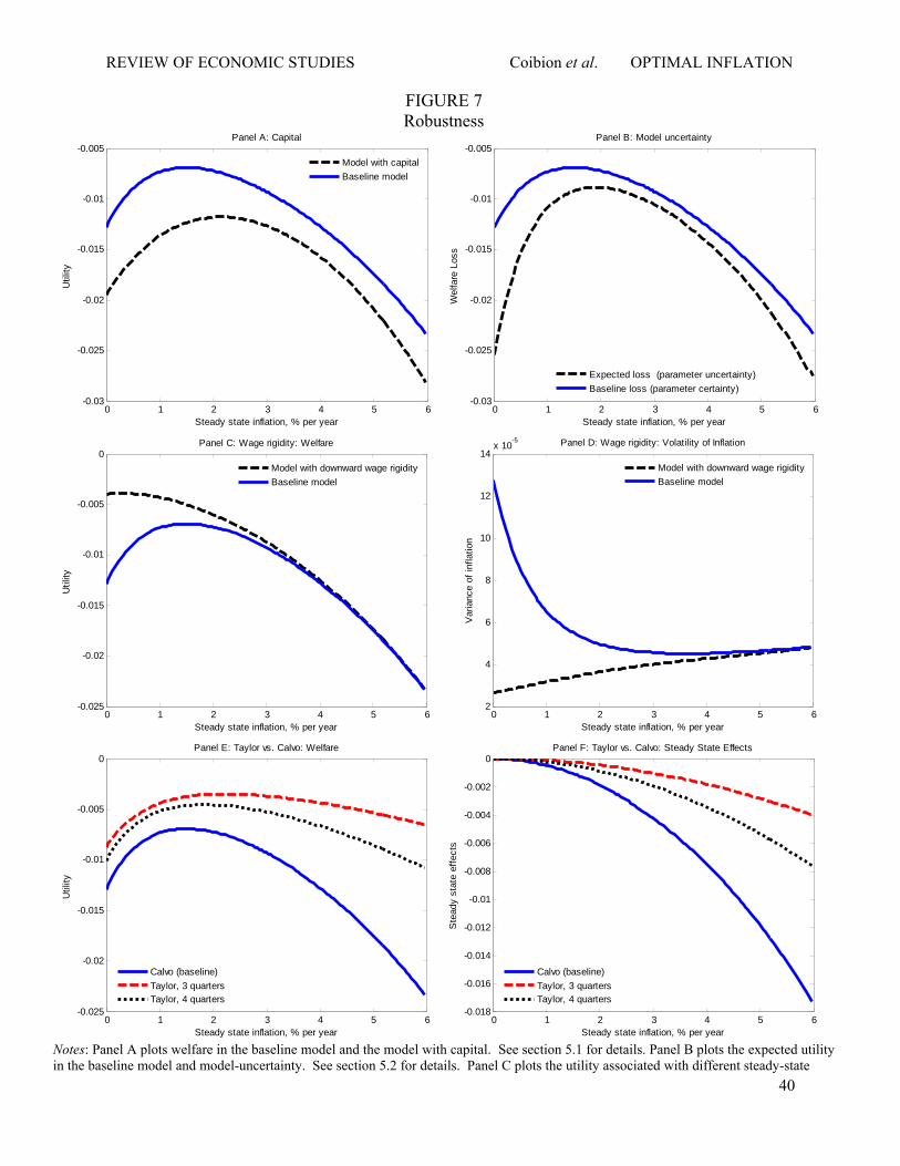
REVIEW OF ECONOMIC STUDIES Coibion et al. OPTIMAL INFLATION
40
FIGURE 7 Robustness
Notes: Panel A plots welfare in the baseline model and the model with capital. See section 5.1 for details. Panel B plots the expected utility in the baseline model and model-uncertainty. See section 5.2 for details. Panel C plots the utility associated with different steady-state
0 1 2 3 4 5 6-0.03
-0.025
-0.02
-0.015
-0.01
-0.005
Steady state inflation, % per year
Util
ity
Panel A: Capital
Model with capital
Baseline model
0 1 2 3 4 5 6-0.03
-0.025
-0.02
-0.015
-0.01
-0.005
Wel
fare
Los
s
Steady state inflation, % per year
Panel B: Model uncertainty
Expected loss (parameter uncertainty)
Baseline loss (parameter certainty)
0 1 2 3 4 5 6-0.025
-0.02
-0.015
-0.01
-0.005
0
Steady state inflation, % per year
Util
ity
Panel C: Wage rigidity: Welfare
Model with downward wage rigidity
Baseline model
0 1 2 3 4 5 62
4
6
8
10
12
14x 10
-5
Steady state inflation, % per year
Var
ianc
e of
infla
tion
Panel D: Wage rigidity: Volatility of Inflation
Model with downward wage rigidity
Baseline model
0 1 2 3 4 5 6-0.025
-0.02
-0.015
-0.01
-0.005
0
Steady state inflation, % per year
Util
ity
Panel E: Taylor vs. Calvo: Welfare
Calvo (baseline)
Taylor, 3 quartersTaylor, 4 quarters
0 1 2 3 4 5 6-0.018
-0.016
-0.014
-0.012
-0.01
-0.008
-0.006
-0.004
-0.002
0
Steady state inflation, % per year
Ste
ady
stat
e ef
fect
s
Panel F: Taylor vs. Calvo: Steady State Effects
Calvo (baseline)
Taylor, 3 quartersTaylor, 4 quarters

REVIEW OF ECONOMIC STUDIES Coibion et al. OPTIMAL INFLATION
41
inflation rates under the baseline model as well as the model with downward nominal wage rigidity. Panel D plots the variance of inflation for different steady-state inflation rates using our baseline model and the model with downward nominal wage rigidity. See section 5.3 for details. Panels E and F plot the implications of Calvo vs. Taylor price setting for welfare. Taylor, X quarters corresponds to the duration of price contracts equal to X quarters. See section 5.4 for details.

REVIEW OF ECONOMIC STUDIES Coibion et al. OPTIMAL INFLATION
42
FIGURE 8 Endogenous and state-dependent price stickiness
Endogenous calvo parameter State-dependent pricing (Dotsey et al. 1999)
0 1 2 3 4 50.45
0.5
0.55
0.6
0.65
0.7
Steady state inflation, % per year
Pric
e S
ticki
ness
()
Panel A
=0
=0.5
=1
0 1 2 3 4 5 60
0.5
1
1.5
2
2.5
3
3.5
4
4.5
5
Steady state inflation, % per year
Ave
rage
dur
atio
n of
pric
e sp
ells
Panel D
= 10
= 7 (baseline)
= 5
0 1 2 3 4 5-0.024
-0.022
-0.02
-0.018
-0.016
-0.014
-0.012
-0.01
-0.008
-0.006
Steady state inflation, % per year
Util
ity
Panel B
=0
=0.5
=1
0 1 2 3 4 5 6-0.06
-0.05
-0.04
-0.03
-0.02
-0.01
0
Steady state inflation, % per year
Util
ityPanel E
= 10
= 7 (baseline)
= 5
0 0.1 0.2 0.3 0.4 0.5 0.6 0.7 0.8 0.9 10
0.5
1
1.5
2
Opt
imal
ste
ady
stat
e in
flatio
n, %
per
yea
r
Sensitivity of frequency of price changes to steady-state inflation,
Panel C
0 0.1 0.2 0.3 0.4 0.5 0.6 0.7 0.8 0.9 1-9
-8
-7
-6x 10
Optimal inflation (left axis)
Welfare loss at optimal inflation
5 5.5 6 6.5 7 7.5 8 8.5 9 9.5 100
0.5
1
1.5
2
Opt
imal
ste
ady-
stat
e in
flatio
n, %
per
yea
r
Elasticity of substition
Panel F
5 5.5 6 6.5 7 7.5 8 8.5 9 9.5 10-0.
-0.
-0.
optimal inflation (left axis)
welfare loss at optimal inflation

REVIEW OF ECONOMIC STUDIES Coibion et al. OPTIMAL INFLATION
43
Notes: The figures plot the implications of endogenous and state-dependent price stickiness on the model. is the effect of steady state inflation on the frequency of price changes 1 . 0 is our baseline case of exogenous price stickiness. See section 5.5 for details.

REVIEW OF ECONOMIC STUDIES Coibion et al. OPTIMAL INFLATION
44
FIGURE 9 Positive implications: optimal policy
Notes: Panels A and B plot outcomes for three scenarios: optimal policy with commitment (Ramsey); optimal policy without commitment (discretion); the baseline Taylor rule described in section 3.1. Optimal policies with and without discretion are described in section 6.1.
0 1 2 3 4 5 6-0.05
-0.045
-0.04
-0.035
-0.03
-0.025
-0.02
-0.015
-0.01
-0.005
0
Steady state inflation, % per year
Util
ity
Panel A: Optimal Policy: Welfare
Commitment
DiscretionBaseline Taylor rule
0 1 2 3 4 5 60
0.05
0.1
0.15
0.2
0.25
0.3
0.35
Steady state inflation, % per year
Fre
quen
cy o
f hi
ttin
g ze
ro lo
wer
bou
nd
Panel B: Optimal Policy: Frequency of hitting ZLB
Commitment
DiscretionBaseline Taylor rule
0 1 2 3 4 5 6-0.03
-0.025
-0.02
-0.015
-0.01
-0.005
0
Steady-state inflation, % per year
Util
ity
Panel C: Taylor rule: Response to inflation
= 2
= 2.5 (baseline)
= 3
= 5
Ramsey
0 1 2 3 4 5 6-0.025
-0.02
-0.015
-0.01
-0.005
0
Steady-state inflation, % per year
Util
ity
Panel D: Taylor rule: Response to output growth rate
g = 0
g = 0.75
g = 1.5 (baseline)
g = 3
Ramsey
0 1 2 3 4 5 6-0.025
-0.02
-0.015
-0.01
-0.005
0
Steady-state inflation, % per year
Util
ity
Panel E: Taylor rule: Response to output gap
y = 0
y = 0.2
y = 0.43 (baseline)
y = 0.6
Ramsey
0 1 2 3 4 5 6-0.025
-0.02
-0.015
-0.01
-0.005
0
Steady-state inflation, % per year
Util
ity
Panel F: Taylor rule: Response to price level gap
p = 0 (baseline)
p = 0.1
p = 0.05
p = 0.25
Ramsey

REVIEW OF ECONOMIC STUDIES Coibion et al. OPTIMAL INFLATION
45
Panels C- F plot the welfare loss as a function of for alternative values of the monetary policy rule parameters. The solid thick blue line corresponds to the baseline parameterization. is the long-run response of interest rates to inflation, is the response to output growth,
is the response to the output gap, and is the response to the price-level gap. See section 6.2 for details.