Agricultural Economics Report No. 187

The North DakotaInput-Output Model:

A Tool for AnalyzingEconomic Linkages

Randal C. CoonF. Larry Lelstrltz

Thor A. HertsgaardArlen G. Leholm

Department of Agricultural EconomicsNorth Dakota Agricultural Experiment Station

North Dakota State UniversityFargo, North Dakota 58105

November 1985

PREFACE

North Dakota's input-output model has become an integral part of manyeconomic research activities involving state issues. Since its development toanalyze the economic impacts associated with irrigation development in the1960s, the model has been updated and used to analyze the effects of a widevariety of projects in North Dakota, Because the model is used and referencedfrequently by economic researchers, the nontechnical audience often requestsadditional information to explain the input-output model and the theory behindit. The purpose of this report is to explain the principles of input-outputanalysis, to describe the structure of the North Dakota model, and to explainhow to interpret the results that might be found in a feasibility or economiccontribution study. This report was designed to be a companion document thatcan be used in conjunction with any report or presentation involving the NorthDakota input-output model.

The authors wish to express their appreciation to Dr. Donald Scott,Dr. William Nelson, and Ms. Brenda Ekstrom for their review of thismanuscript. The authors also would like to gratefully acknowledgecontributions of Ms. Jody Peper for typing the report, and various facultymembers of the Department of Agricultural Economics for their reviews andsuggestions.

Table of Contents

List of Tables . . . . . . . . . . . . . . .

List of Figures . . . . . . . . . . .

Highlights . . . . . . . . . . . . . .

Introduction * * * * * . . . .

Input-Output Theory . .......... . .Mathematical Representation . . . . . . .Hypothetical Economy . . . . . . . . . . .

Transactions Table . . . . . . . . . . .Technical Input-Output Coefficients Table .Interdependence Coefficients Table . . .

Assumptions and Limitations . . . . . .

History of the North Dakota Input-Output Model

North Dakota Input-Output Model . . . . . .North Dakota Sales for Final Demand . . .North Dakota Gross Business Volumes . . .North Dakota Productivity Ratios . . . .. .Tax Revenue Estimation . . . . .. . . . . .

Regional Input-Output Model . . . . . . .

Uses of Input-Output Analysis in North DakotaExamples of Input-Output Analysis . . . . .Interpreting the Results of an Economic Impact

Summary . . . . . . . . . . . . . .

Appendix A . . . . . . . . . . . . . .

Appendix B . . . . . . . . . . . . . . . . . .

References . . . . . . . . . . . . . .

0 0 0 0 0 0

0 0 0 0 0 0

S. Assessment

. . . . . .

. . . . . .

. . . . . .

. . . . . .

. . . . . .

. . . . . .

. . . . . .

. . . . . .

. . . . . .

. . . . . .

. . . . . .

. . . . . .

. . . . . .

Assessment

. . . . . .

. . . . . .

. . . . . .

. . . . . .

O

B

O

O

Page

. ii111

. iii

. 1

S 2S 3

. 6S 7S 8S 9

. 11

. 11

S 13S 20S 23S 23

. 28

S 29

S 30S 32S 33

S 39

S 41

S 45

S 51

List of Tables

Table Page

1. MATHEMATICAL REPRESENTATION OF A TRANSACTIONS TABLE FOR AHYPOTHETICAL THREE-SECTOR EXPORT-BASED ECONOMIC SYSTEM . . . . . . 4

2. MATHEMATICAL REPRESENTATION OF A TECHNICAL INPUT-OUTPUTCOEFFICIENTS TABLE FOR A HYPOTHETICAL THREE-SECTOR EXPORT-BASEDECONOMIC SYSTEM . . . . . . . . . . . . . . . . . . . . . .. . .5

3. MATHEMATICAL REPRESENTATION OF INPUT-OUTPUT INTERDEPENDENCECOEFFICIENTS TABLE FOR A HYPOTHETICAL THREE-SECTOR EXPORT-BASEDECONOMIC SYSTEM ...... . . .......... . ... . . 6

4. TRANSACTIONS TABLE FOR A HYPOTHETICAL THREE-SECTOR EXPORT-BASEDECONOMIC SYSTEM. ............... . ..... ..... . .. ..... 7

5. TECHNICAL INPUT-OUTPUT COEFFICIENTS FOR A HYPOTHETICALTHREE-SECTOR EXPORT-BASED ECONOMIC SYSTEM .... .. . . . . . . .

6. INPUT-OUTPUT INTERDEPENDENCE COEFFICIENTS TABLE FOR AHYPOTHETICAL THREE-SECTOR EXPORT-BASED ECONOMIC SYSTEM. . .. .. 9

7. ECONOMIC SECTORS AND ASSOCIATED STANDARD INDUSTRIALCLASSIFICATION CODES FOR THE NORTH DAKOTA INPUT-OUTPUT MODEL . . . 14

8. INPUT-OUTPUT TECHNICAL COEFFICIENTS FOR 17-SECTOR MODEL, NORTHDAKOTA . . . . . . . . . . . . . . . . . . . . . . . . . . . . . 15

9. INPUT-OUTPUT INTERDEPENDENCE COEFFICIENTS, BASED ON TECHNICALCOEFFICIENTS FOR 17-SECTOR MODEL, NORTH DAKOTA.. ......... . 17

10. SALES FOR FINAL DEMAND, BY ECONOMIC SECTOR, NORTH DAKOTA,(CURRENT DOLLARS), MILLION DOLLARS, 1958-1984. ... .. . . .. . . 21

11. GROSS NATIONAL PRODUCT IMPLICIT PRICE DEFLATORS FOR 1980 BASE . . 2212. GROSS BUSINESS VOLUMES OF ECONOMIC SECTORS ESTIMATED BY THE

INPUT-OUTPUT MODEL, NORTH DAKOTA, MILLION DOLLARS, 1958-1984 . . . 2413. ESTIMATES OF PERSONAL INCOME AND DIFFERENCES IN ESTIMATES, NORTH

DAKOTA, 1958-1984 (THOUSAND DOLLARS) . . . .......... . 2514. EMPLOYMENT BY ECONOMIC SECTOR, NORTH DAKOTA, 1958-1984 . . .. . . 2615. GROSS BUSINESS VOLUME TO EMPLOYMENT (PRODUCTIVITY) RATIOS, BY

ECONOMIC SECTOR, NORTH DAKOTA, 1958-1984 ..... ... .. .. 2716. COMPARISON OF STATISTICAL TESTS FOR THE INPUT-OUTPUT MODEL

PERSONAL INCOME ESTIMATION, NORTH DAKOTA REGIONS 1-8 AND STATE,1958-1984 . . . . . . . . . . . . . . . . . . . . . . . . . . . . 31

List of Figures

Figure

1. North Dakota State Planning Regions .... . ........ . 29

ii

Highlights

Tnput-output (I-0) analysis is a technique for describing the linkagesor interdependencies among the various sectors within an economy. Thistechnique has been employed to quantitatively describe the North Dakotaeconomy. Development of the North Dakota I-0 model followed a three-stepapproach. First, a transactions table was constructed showing the purchasesand sales by each sector of the economy to each of the other industrialsectors. Next, the technical input-output coefficients table was derived fromthe transactions table. This technical coefficients table is the transactionstable expressed as decimal fractions of the column totals in the transactionstable. Finally, the input-output interdependence coefficients, ormultipliers, table was derived from the technical input-output coefficentstable.

Development of the North Dakota I-0 model has taken place over a20-year period. The first attempt to study the intersector relationships of alocal community in the state was conducted in Ransom County in 1963. A surveyof seven southwestern counties was initiated in 1966 for the purpose ofdeveloping an input-output model. This model was primarily used to analyzethe economic impacts associated with development of the Garrison Diversionirrigation project. The model was tested and validated for use at the stateand substate levels. As energy development became important in the state, themodel was expanded to include coal mining, thermal-electric power generation,petroleum exploration/extraction, and petroleum refining.

North Dakota's economic base is comprised of those activities producingeither a product paid for by nonresidents or products exported from the state.Included in these economic base activities are agriculture (livestock and cropproduction plus government payments for agricultural programs), mining,manufacturing, tourist expenditures for retail purchases and business andpersonal services, and federal government outlays for construction and toindividuals. Application of the input-output interdependence coefficients tothe estimated levels of basic economic activities, or sales for final demand,yields estimates of gross business volume. These values indicate the totaldollar volume of business activity occurring after the multiplier process hasbeen completed.

The North Dakota I-0 model has been used to analyze the economicimpacts associated with a wide range of issues in the state. Studies involvedwith irrigation, coal and other energy development, feasibility, contribution,recreation, government programs, and comprehensive socioeconomic modeldevelopment have all relied heavily on the input-output model's economicestimates. The model has been used to determine the effects of a wide varietyof industrial and agricultural developments in the state. Analyzing impactsassociated with these developments using the input-output model has proven tobe accurate and beneficial for those requiring this type of information.

iii

THE NORTH DAKOTA INPUT-OUTPUT MODEL: A TOOLFOR ANALYZING ECONOMIC LINKAGES

by

Randal C. Coon, F. Larry Leistritz, Thor A. Hertsgaard, and Arlen G. Leholm*

Introduction

North Dakota's economy is composed of basic activities that areprimarily resource based, i.e., involving either energy or agriculturalproduction (although manufacturing, tourist expenditures, and federalgovernment outlays also are included). To better understand the basiccomponents of the state's economy and the interdependencies among thesecomponents, input-output (1-0) analysis techniques have been used.Input-output analysis can be used to quantitatively describe and analyze theinterrelationships (economic linkages) within a state or regional economy.

Basic economic activities are defined as those that bring dollars intoa state or region in return for exported products. For example, suppose thata small regional economy such as a small farming community produces a product(e.g., crop production) which is shipped from the area. The producers receivemoney payments from outside the area and use part of those payments to pay forthe inputs used in producing the product; these costs are, in turn, revenuesto the secondary businesses that serve and support the crop production sector.The survival of an economic unit depends on its ability to produce productsand sell them at a price that is high enough to pay all costs of production,including the market value of the use of the producer's own resources. Thepayments the firm makes to other firms for inputs purchased from them arerevenues to trade and service industries. If the basic industry expands,there will be a demand for additional output from the trade and servicebusinesses, and vice versa if the basic industry shrinks.

An I-0 model has been developed for North Dakota to quantitativelydescribe the economy at the state and substate (i.e., state planning region)levels. This model has been used extensively for such economic analyses asstudies of the economic contribution of specific sectors of the state'seconomy, evaluation of the impact of expansion or contraction of a given basicsector, secondary employment estimation, and state tax revenue estimation. Inaddition, the I-0 model is one of the basic components of an integratedeconomic-demographic model that projects income, employment, population, andrelated variables based on relationships to its central feature, the I-0model.

Because the I-0 model is used so often by economic researchers, it hasbeen referenced extensively but has seldom, if ever, been fully explained tothe nontechnical audience. The purpose of this report is to explain the

*Coon is research specialist, Leistritz, and Hertsgaard are professors,Department of Agricultural Economics, and Leholm is associate professor,Extension Agricultural Economics, North Dakota State University.

- 2-

principles of input-output analysis, to describe the structure of the NorthDakota model, and to explain how to interpret the results that may appear in afeasibility or economic contribution study. This report was designed to be acompanion document that can be used in conjunction with any report orpresentation involving the North Dakota input-output model; it provides thereference material necessary to understand input-output analysis as it relatesto the state's economy.

Remaining sections of this report cover I-0 theory, history of theNorth Dakota I-0 model, I-0 data tables, applications of the model, andexamples of the way in which the model has been used. A glossary ofterminology relating to input-output analysis is presented in Appendix A.

Input-Output Theory

Input-output concepts had their roots in the early development ofeconomic theory. In 1758 Francois Quesnay published Tableau Economique, whichstressed the interdependence of economic activities (for a discussion ofQuesnay's work, see Newman [1952]). Quesnay's original model depicted theoperation of a single farm and showed successive "rounds" of wealth-producingactivity that resulted from a given increase in agricultural output.Essentially, this was the forerunner of the modern multiplier concept. Thenext step in the development of input-output theory did not come until 1874when Leon Walras published Elements d'economic politique pure. The modeldeveloped by Walras showed interdependence among producing sectors of theeconomy and the competing demands of each sector for the factors ofproduction. His system also included equations representing consumer incomeand expenditure, and it allowed consumers to substitute the products of onesector for those produced by another.

Professor Wassily Leontief of Harvard University developed a generaltheory of production based on the notion of economic interdependence. Hepublished the first input-output table for the American economy, showing howeach sector of the economy was dependent upon each other sector. For acomplete discussion of Leontief's work with input-output, see Leontief (1966).Since Leontief's first input-output table, interindustry analysis has becomean important branch of economics. Input-output tables are uted on a nationallevel throughout the world, and in the United States many state and substateI-0 models have been developed. Miernyk (1967) provides a detailed review ofthe history of input-output analysis and a discussion of its applications(Mi er-nyk-4If982),.

Input-output analysis is a technique for tabulating and describing thelinkages or interdependencies between various industrial groups within aneconomy. The economy considered may be the national economy or an economy assmall as that of a multicounty area served by one of the state's major retailtrade centers. The analysis assumes that economic activity in a region isdependent upon the "basic" industries that exist in the area, referred to asits economic base. The North Dakota economy is largely export-based (i.e., itconsists of those industries or "basic" sectors that earn income from outsidethe area). Remaining activities are the trade and service sectors (orindustries) which exist to provide the inputs requiredby other sector s in thearea.

-3-

Production by any sector requires the use of production inputs, such asmaterials, equipment, fuel, services, labor, etc., by that sector. Theseinputs are referred to as the direct requirements of that sector. Some ofthese inputs will be obtained from outside the region (imported), but manywill be produced by and purchased from other sectors in the area economy. Ifthe latter is true, these other sectors will require their own inputs fromstill other sectors, which in turn will require inputs from yet other sectors,and so on. These additional rounds of input requirements that are generatedby production of the direct input requirements (of the initial sector) areknown as the indirect requirements.

The total of the direct and indirect input requirements of each sectorin an economy is measured by a set of coefficients that is known as theinput-output interdependence coefficients. Development of these coefficientsfollows a three-step approach. First, a transactions table is constructedshowing the purchases and sales by each of the sectors to each of the otherindustrial sectors. This table is arranged so columns show the purchases from(and payments to) each row sector, and the rows indicate the sales of that rowsector to the column sectors.

Next, the technical input-output coefficients table is derived from thetransactions table. The technical coefficients table is the transactionstable expressed as decimal fractions of column totals in the transactionstable. Thus, each coefficient in that table indicates the fraction of totalinputs of the column sector that is obtained from the row sector. In otherwords, each coefficient indicates the direct requirements (per dollar ofoutput) that the column sector obtains from the row sector.

Finally, the interdependence coefficients (multipliers) table isderived from the technical input-output coefficients table. Theinterdependence coefficients table shows the total input requirements (directand indirect) that must be obtained from the row sector per dollar of outputfor final demand by the column sector. Each coefficient includes the directinput requirement from the transactions table, the indirect input requirementsdue to the multiplier effect, and, if appropriate, output for final demand bythe column sector. The column totals of this table are the total outputrequirements of all row sectors in the economy per dollar of output for finaldemand by the column sector. These column totals are calledgross receipts,multipliers.

Mathematical Representation

An example of a hypothetical economy will be presented and discussed tofurther illustrate input-output theory. Assume the local economy in thisexample is the state (although it could be a substate region, a multistateregion, or the nation.) An industry (or economic sector) can be defined as agrouping of business firms producing similar products. (Government andhouseholds are often defined as economic sectors; both are included in theNorth Dakota model. The household sector earns personal income in the form ofrent, interest, wages and salaries, and profits.) For any industry, totalvalue of output (sales) over a particular time period equals the sum of itssales to each local industry plus. its sales in markets .outside the state.That is, for n delineated sectors in the state,

-4-

n(1) Yi ==

j=1Tij + Zi i,j = 1, , ... , n

Yi = total output for sector iToj = in-state sales to sector j by sector i (endogenous transactions)Zi = out-of-state sales by sector i (exogenous transactions)

Equation 1 can be represented in tabular form as presented in Table 1. TheTi u's denote endogenous transactions or in-state transactions occurring amongindustries of the model. Each Tij indicates a sale by the ith industry to thejth industry. Conversely, Tij can also show a purchase by the jth industryfrom the it" industry. Thus, columns represent purchases while rows showsales. In Table 1, the Zi section shows exports (exogenous transactions), andthe Yi section indicates total output or total sales.

Table 1 represents a complete economic system. An import, or nonlocalinput row has been added to the transactions table to show a complete pictureof all transactions. By adding this row to the transactions table, totalinputs equal total output, and the economy described becomes a completeeconomic system. In Table 1, EZ represents total exports by all industries,

TABLE 1. MATHEMATICAL REPRESENTATION OF A TRANSACTIONS TABLE FOR AHYPOTHETICAL THREE-SECTOR EXPORT-BASED ECONOMIC SYSTEM

Selling Purchasing Sector TotalSector Industry #1 Industry #2 Industry #3 Exports Output

Industry #1 T11 T12 T13 Z1 Y1

Industry #2 T2 1 T22 T23 Z2 Y2

Industry #3 T3 1 T32 T33 Z3 Y3

Imports W1 W2 W3

Total Input Y1 Y2 Y3 SZ EoT + 4(or ••T + SZ)

summation of all elements in the row (including exports) equals total outputby all industries, SW is the total imports, and column totals are total inputsof that sector. If households are not a sector that is included in the model,resource payments (in the form of rent, interest, salaries and wages, andprofits) to households are included as a part of the import row. Thus,because resource payments to households are included in each column (either in

where:

-5-

the household row or as a part of themust equal its total output. This ishouseholds is the balancing componentequal total output for each sector.

import row), total input of each sectortrue because profit or loss ofof gross input that makes total input

An input-output technical coefficients table can be derived from thetransactions table based on the following relationship.

Tij(2) aij ="

Yj

An example technical coefficients table with mathematical representation(Table 2) shows the aij's and the other ratios; although only the aij's are

TABLE 2. MATHEMATICAL REPRESENTATION OF A TECHNICAL INPUT-OUTPUT COEFFICIENTSTABLE FOR A HYPOTHETICAL THREE-SECTOR EXPORT-BASED ECONOMIC SYSTEM

Selling Purchasing SectorSector Industry #1 Industry #2 Industry #3

Industry #1 all a12 a13

Industry #2 a21 a22 a23

Industry #3 a31 a32 a33

Imports WI/Y 1 W2/Y2 W3/Y3

Total 1.00 1.00 1.00

functional, the others are presented for descriptive purposes. The ainsegment of Table 2 is used to calculate the interdependence coefficients ormultipliers. Substituting equation 2 into equation 1 results in

n(3) Yi = aij Yj + Zi j = 1, 2, . .. , n

j=1

Put in matrix notation, this relationship becomes

(4)(5)(6)(7)(8)(9)

Y = AY + ZY - AY = Z[I-A]Y = Z[I-A-1[I-AY = [I-A]-IY = [I-A] ZY = [I-A]- 1Z

Each element of the [I-A]- 1 denotes the amount of output from the ith industrythat is required either directly or indirectly per unit of output by the jthindustry for export from the state. Table 3 shows a common format for

TABLE 3. MATHEMATICAL REPRESENTATION OF INPUT-OUTPUT INTERDEPENDENCECOEFFICIENTS TABLE FOR A HYPOTHETICAL THREE-SECTOR EXPORT-BASEDECONOMIC SYSTEM

Selling Purchasing SectorSector Industry #1 Industry #2 Industry #3

Industry #1 mil m1 2 m13

Industry #2 m2 1 m22 m2 3

Industry #3 m3 1 m32 m33

Total Multipliers M1 M2 M3

presenting the inverse matrix. Each element (mij) is a multiplier indicatingboth the direct and indirect effect upon the "row industry" of basic incomereceived by the "column industry." Summing the columns produces a multiplier(Mi) denoting the dollar value of output of all sectors that results per dollarof export by the "column industry." This multiplier is often referred to as thegross receipts multiplier. For a more detailed discussion of input-outputtheory, mathematics, and formula derivation, see Harmston and Lund (1967).

Hypothetical Economy

An example of how the multipliers would be derived for a hypotheticalthree-sector economy will further illustrate how input-output theory has beenput to practical use. This economy consists of three sectors: Agriculture(Agr), Manufacturing (Mfg), and Trade and Service (T&S). Firms in each sectorrequire inputs (the output of firms in other sectors) and also produce outputs(the inputs of firms in other sectors). As previously mentioned, three typesof tables are involved in input-output analysis: (1) the transactions table,(2) the technical input-output coefficients table, and (3) the table ofinterdependence coefficients. Development of multipliers will be tracedthrough the three-step process of constructing the above mentioned tables. Anextensive discussion of mathematical procedures will not be repeated, butrather an explanation of the interpretation of the tables will be addressed.

- 6 -

-7-

Transactions Table

This table contains the basic data from which the other two tables arederived. This transactions table is simply a table showing the receipts (orpayments) of each economic sector (group of similar economic units) to (orfrom) each other sector. The table is arranged so the columns show theexpenditures of each sector to the row sectors and the rows indicate thereceipts of each sector from the column sectors. Hypothetical data for thethree-sector economy are presented in Table 4. The dollar volumes in the

TABLE 4. TRANSACTIONS TABLE FOR A HYPOTHETICAL THREE-SECTOR EXPORT-BASEDECONOMIC SYSTEM

Selling Purchasing Sector TotalSector (1) Agr (2) Mfg (3) T&S Exports Output

- - - -- ----- --- -million dollars----------

(1) Agr 6 7 16 71 100

(2) Mfg 4 13 8 25 50

(3) T&S 60 10 12 118 200

Imports 30 20 164

Total Input 100 50 200

column sectors refer to production inputs purchased from each row sector;these purchases are also sales of output to the column sector from the rowsectors. For example, the 6 in the row 1, column 1, represents a purchase of$6 million of inputs by farmers from other farmers as well as a sale of $6million of the agricultural sector's output to farmers. The 4 in row 2 of theagriculture column reflects $4 million of inputs purchased by farmers from themanufacturing sector. Additionally, the 60 in row 3 column 1, represents asale of $60 million from the trade and service sector to the agriculturesector, the 10 in row 3 and the 12 in row 3 represent sales of $10 million and$12 million from the trade and service sector to the manufacturing and tradeand service sectors, respectively.

All transactions among sectors 1, 2, and 3 are for intermediateproducts; that is, these transactions are for inputs to be used in additionalstages of production. On the other hand, the exports (or sales for finaldemand) column in Table 4 represents sales of final products. These salescould be to households for personal consumption, to business firms for capitalinvestment, or to the various governmental units, or they could be exportsoutside the local economy. The row entitled imports is the counterpart to thecolumn exports. Imports include wages and salaries, profits or losses, rent,

-8-

interest payments to people, depreciation allowances for capital investments,tax payments to government, and imports from outside the local economy. Theprofit or loss in row 4 is the residual which equates gross receipts and grossexpenditures. Therefore, the column total is equal to the row total for agiven sector.

Technical Input-Output Coefficients Table

The technical input-output table (also referred to as the directrequirements table or the A matrix) is simply the transactions matrixexpressed as decimal fractions of column totals. Each coefficient in thistable indicates the fraction of total inputs of the column sector obtainedfrom the row sector. Alternatively stated, each coefficient indicates thedirect requirements (per dollar of output) that the column sector obtains fromthe row sector.

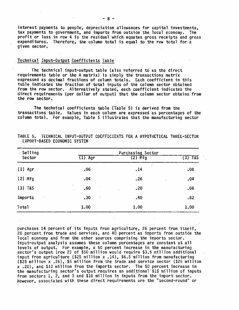
The technical coefficients table (Table 5) is derived from thetransactions table. Values in each column are expressed as percentages of thecolumn total. For example, Table 5 illustrates that the manufacturing sector

TABLE 5. TECHNICAL INPUT-OUTPUT COEFFICIENTS FOR A HYPOTHETICAL THREE-SECTOREXPORT-BASED ECONOMIC SYSTEM

Selling Purchasing SectorSector (1) Agr (2) Mfg (3) T&S

(1) Agr .06 .14 .08

(2) Mfg .04 .26 .04

(3) T&S .60 .20 .06

Imports .30 .40 .82

Total 1.00 1.00 1.00

purchases 14 percent of its inputs from agriculture, 26 percent from itself,20 percent from trade and services, and 40 percent as imports from outside thelocal economy and from the other sources comprising the imports sector.Input-output analysis assumes these column percentages are constant at alllevels of output. For example, a 50 percent increase in the manufacturingsector's output (row 2) of $50 million would require $3.5 million additionalinput from agriculture ($25 million x .14), $6.5 million from manufacturing($25 million x .26), $5 million from the trade and service sector ($25 millionx .20), and $10 million from the imports sector. The 50 percent increase inthe manufacturing sector's output requires an additional $15 million of inputsfrom sectors 1, 2, and 3 and $10 million in inputs from the import sector.However, associated with these direct requirements are the "second-round" or

-9-

indirect and induced input requirements. The $3.5 million of additional inputfrom agriculture implies that farm output must be increased by that amount,which in turn will require increased inputs in agriculture. The"second-round" or indirect and induced impacts can be found by applying thetechnical input-output coefficients from Table 5, column 1, to the required$3.5 million of expanded agricultural output. Second-round input requirementsare $.21 million from other farms, $.14 million from the manufacturing sector,and $2.10 million from the trade and service sector. Increased output fromthese second-round effects will generate additional waves of inputrequirements (third, fourth, and subsequent rounds) resulting in the familiarmultiplier effect. The second-, third-, fourth-, and all subsequent-roundeffects are included along with the direct effects measured by the technicalcoefficients in the interdependence coefficients (described in the nextsection).

Interdependence Coefficients Table

The interdependence coefficients (multiplier) table (Table 6) isderived from the technical input-output coefficients table. Computationally,

TABLE 6. INPUT-OUTPUT INTERDEPENDENCE COEFFICIENTS TABLE FOR A HYPOTHETICALTHREE-SECTOR EXPORT-BASED ECONOMIC SYSTEM

Selling Purchasing SectorSector (1) Agr (2) Mfg (3) T&S

(1) Agr 1.1430 .2454 .1077

(2) Mfg .1024 1.3891 .0678

(3) T&S .7514 .4522 1.1470

Total Multipliers 1.9968 2.0867 1.3225

it is the inverse of the I-A matrix, or [I-A]- 1. It shows the total (directand indirect) input requirements that must be obtained from the row sector perdollar of output for final demand by the column sector. Each coefficientincludes the direct input requirement (from the technical coefficients ordirect requirements table) and the indirect input requirement (resulting fromthe multiplier effect). Column totals of this table are the total outputrequirements of all the row sectors per dollar of output for export (or finaldemand) by the column sector. These column totals are called gross receiptsmultipliers.

- 10 -

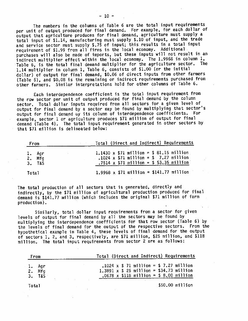
The numbers in the columns of Table 6 are the total input requirementsper unit of output produced for final demand. For example, for each dollar ofoutput that agriculture produces for final demand, agriculture must supply atotal input of $1.14, manufacturing must supply $.10 of input, and the tradeand service sector must supply $.75 of input; this results in a total inputrequirement of $1.99 from all firms in the local economy. Additionalpurchases will also be made of imports, but these inputs will not result in anindirect multiplier effect within the local economy. The 1.9968 in column 1,Table 6, is the total final demand multiplier for the agriculture sector. The1.14 multiplier in column 1, Table 6, consists of $1.00 (or the initialdollar) of output for final demand, $0.06 of direct inputs from other farmers(Table 5), and $0.08 is the remaining or indirect requirements purchased fromother farmers. Similar interpretations hold for other columns of Table 6.

Each interdependence coefficient is the total input requirement fromthe row sector per unit of output produced for final demand by the columnsector. Total dollar inputs required from all sectors for a given level ofoutput for final demand by a sector may be found by multiplying that sector'soutput for final demand uy its column of interdependence coefficients. Forexample, sector 1 or agriculture produces $71 million of output for finaldemand (Table 4). The total input requirement generated in other sectors bythat $71 million is delineated below:

From Total (Direct and Indirect) Requirements

1. Agr 1.1430 x $71 million = $ 81.15 million2. Mfg .1024 x $71 million = $ 7.27 million3. T&S .7514 x $71 million = $ 53.35 million

Total 1.9968 x $71 million = $141.77 million

The total production of all sectors that is generated, directly andindirectly, by the $71 million of agricultural production produced for finaldemand is $141.77 million (which includes the original $71 million of farmproduction).

Similarly, total dollar input requirements from a sector for givenlevels of output for final demand by all the sectors may be found bymultiplying the interdependence coefficients for that row sector (Table 6) bythe levels of final demand for the output of the respective sectors. From thehypothetical example in Table 4, these levels of final demand for the outputof sectors 1, 2, and 3, respectively, are $71 million, $25 million, and $118million. The total input requirements from sector 2 are as follows:

From Total (Direct and Indirect) Requirements

1. Agr .1024 x $ 71 million = $ 7.27 million2. Mfg 1.3891 x $ 25 million = $34.73 million3. T&S .0678 x $118 million = $ 8.00 million

$50.00 millionTotal

- 11 -

The total of $50.00 million of gross input from sector 2 is (and should be)identical to its gross receipts recorded in the transactions table (Table 4).

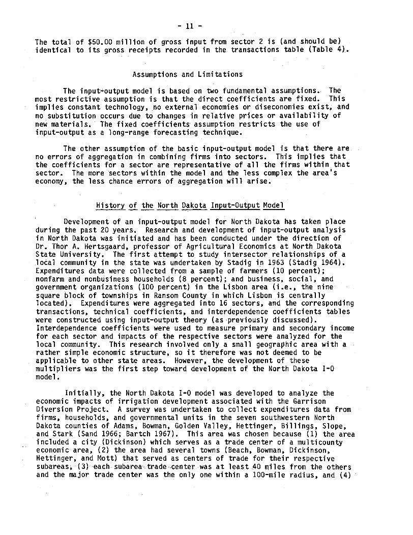
Assumptions and Limitations

The input-output model is based on two fundamental assumptions. Themost restrictive assumption is that the direct coefficients are fixed. Thisimplies constant technology, no external economies or diseconomies exist, andno substitution occurs due to changes in relative prices or availability ofnew materials. The fixed coefficients assumption restricts the use ofinput-output as a long-range forecasting technique.

The other assumption of the basic input-output model is that there areno errors of aggregation in combining firms into sectors. This implies thatthe coefficients for a sector are representative of all the firms within thatsector. The more sectors within the model and the less complex the area'seconomy, the less chance errors of aggregation will arise.

History of the North Dakota Input-Output Model

Development of an input-output model for North Dakota has taken placeduring the past 20 years. Research and development of input-output analysisin North Dakota was initiated and has been conducted under the direction ofDr. Thor A. Hertsgaard, professor of Agricultural Economics at North DakotaState University. The first attempt to study intersector relationships of alocal community in the state was undertaken by Stadig in 1963 (Stadig 1964).Expenditures data were collected from a sample of farmers (10 percent);nonfarm and nonbusiness households (8 percent); and business, social, andgovernment organizations (100 percent) in the Lisbon area (i.e., the ninesquare block of townships in Ransom County in which Lisbon is centrallylocated). Expenditures were aggregated into 16 sectors, and the correspondingtransactions, technical coefficients, and interdependence coefficients tableswere constructed using input-output theory (as previously discussed).Interdependence coefficients were used to measure primary and secondary incomefor each sector and impacts of the respective sectors were analyzed for thelocal community. This research involved only a small geographic area with arather simple economic structure, so it therefore was not deemed to beapplicable to other state areas. However, the development of thesemultipliers was the first step toward development of the North Dakota I-0model.

Initially, the North Dakota I-0 model was developed to analyze theeconomic impacts of irrigation development associated with the GarrisonDiversion Project. A survey was undertaken to collect expenditures data fromfirms, households, and governmental units in the seven southwestern NorthDakota counties of Adams, Bowman, Golden Valley, Hettinger, Billings, Slope,and Stark (Sand 1966; Bartch 1967). This area was chosen because (1) the areaincluded a city (Dickinson) which serves as a trade center of a multicountyeconomic area, (2) the area had several towns (Beach, Bowman, Dickinson,Hettinger, and Mott) that served as centers of trade for their respectivesubareas, (3) each subarea trade center was at least 40 miles from the othersand the major trade center was the only one within a 100-mile radius, and (4)

- 12 -

the area was primarily agricultural with both small grain and livestockenterprises. The major problem encountered was the cost of undertaking suchan extensive data-gathering effort. However, data were collected, and a30-sector input-output model was developed. The resultant multipliers wereused to evaluate the role of a region's trade center and to estimate theimpact of the Garrison Diversion Unit.

The original 30-sector input-output model was later delineated into 21economic sectors, and the interdependence coefficients were derived (Lutovsky1968). Primary income of the basic sectors in the economy, or sales for finaldemand, were applied to the interdependence coefficients to estimate grossincome of each sector. North Dakota was divided into 12 trade areas, andpublished estimates of state personal income were disaggregated to correspondwith the trade areas. Estimates of personal income obtained from the twosources were compared for differences at the state and trade area levels.Results of the comparisons were favorable; all but two trade areas hadpercentage differences less than 11 percent, and the state difference was 5.41percent for 1960. The conclusion was drawn that the interdependencecoefficients could be used for economic analysis for other trade areas and atthe state level with an acceptable degree of accuracy.

Subsequently the interdependence coefficients were evaluated forreliability over a longer time period (1958-1968) by determining sales forfinal demand for each year during the period and applying these values to thecoefficients to obtain estimates of personal income (Senechal 1971). For thisanalysis the state was divided into eight regions and personal income wasdisaggregated to correspond to these regions. Methodology for estimatingincome from basic economic sectors (or sales for final demand) was developed,and final demand vectors were calculated for each basic sector and stateregion for 1958 to 1968. These final demand vectors were applied to theinterdependence coefficients to estimate gross business volume and personalincome at the state and regional levels. Personal income estimates at thestate level were very accurate, and substate estimates were reliable withincertain limitations. Conclusions from this study were that theinterdependence coefficients developed in southwestern North Dakota were validfor other parts of the state and that the model should be aggregated intofewer sectors.

Accordingly, the I-0 model was aggregated into a 13-sector model andremained unchanged for many years. As previously mentioned, the principalintended use for which input-output coefficients initially were assembled inNorth Dakota was for projecting the economic impacts of irrigation developmentin the state. However, since the data were collected, a wide variety ofapplications has been made. The major use of the model during the 1970s wasfor estimating the economic impacts of coal resource development.

The model developed from the original expenditures data had only onesector to describe the various mining activities within the state. Thissector reflected the characteristics of firms in southwestern North Dakotathat were engaged in sand and gravel mining but did not include suchactivities as coal and petroleum mining. The omission of coal and petroleummining was not a serious deficiency in the model as long as the majorcomponent of the state's economic base was agriculture and as long as therewere no important interdependencies of other economic sectors with coal and

- 13 -

petroleum mining. However, the increasing importance of mining as a componentof the state's economic base and the prospects for accelerated development ofcoal conversion facilities in the state resulted in a need for more detailedinput-output data for the energy sectors.

Collection of expenditures data in North Dakota from firms in fouradditional sectors related to energy production was undertaken in 1975(Hertsgaard et al. 1976). These sectors were coal mining, thermal-electricpower generation, petroleum and natural gas extraction, and petroleumrefining. Expenditures data for the energy-related industries were used toobtain technical coefficients for the four additional economic sectors. Thesecoefficients were appended to the technical coefficients for the 13-sectormodel to obtain a 17 by 17 matrix of technical coefficients for the 17-sectormodel. The interdependence coefficients for the 17-sector model were thencomputed by inverting the [I-A] matrix of that model.

The 17-sector I-0 model has been used extensively since its developmentand has been especially useful for analyzing impacts resulting from energydevelopment. Energy development in the state has declined considerably since1983, but the I-0 model has been used for other purposes, such as economiccontribution studies and analysis of impacts associated with industrialdevelopment in the state. Although the model has not been changed in recentyears, it is possible to adjust the I-0 model to reflect changes in thestate's economic base. This process involves collecting expenditures data andaugmenting the current I-0 matrix as previously discussed. Changing andrefining the North Dakota I-0 model over time has made it more accurate anduseable and gives a good indication of its importance to researchers foreconomic analyses, such as forecasting, contribution studies, and impactanalysis.

North Dakota Input-Output Model

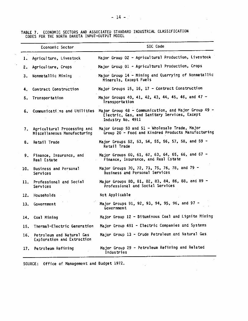
The current version of the North Dakota I-0 model groups the state'seconomy into 17 industrial classifications, -or sectors. Sector delineationsand corresponding Standard Industrial Classifications (SIC) are presented inTable 7. These groupings were used to identify expenditures (i.e.,transactions table) and basic economic sectors. Thus, input-outputinterdependence coefficients and sales for final demand were determinedaccording to these categories.

Expenditures data previously gathered (Sand 1966; Bartch 1967;Hertsgaard et al. 1976) were the basis for the current I-0 model'stransactions table. Using methodology previously discussed, the transactionstable was converted into an input-output technical coefficients table for theNorth Dakota economy (Table 8). Input-output interdependence coefficients(multipliers) were derived from the technical coefficients by inverting theI-A matrix, or computationally [I-A]- 1 . The resultant 17-sector North Dakotainput-output interdependence coefficients are presented in Table 9.

Although the input-output interdependence coefficients have beendiscussed in great detail in an earlier section of this report, a briefexplanation of the North Dakota multipliers will be presented to facilitate

- 14 -

TABLE 7. ECONOMIC SECTORS AND ASSOCIATED STANDARD INDUSTRIAL CLASSIFICATIONCODES FOR THE NORTH DAKOTA INPUT-OUTPUT MODEL

Economic Sector SIC Code

1. Agriculture, Livestock

2. Agriculture, Crops

3. Nonmetallic Mining

4. Contract Construction

5. Transportation

6. Communicati ns and Utilities

7. Agricultural Processing andMiscellaneous Manufacturing

8. Retail Trade

9. Finance, Insurance, andReal Estate

10. Business and PersonalServices

11. Professional and SocialServices

12. Households

13. Government

14. Coal Mining

15. Thermal-Electric Generation

16. Petroleum and Natural GasExploration and Extraction

17. Petroleum Refining

Major Group 02 - Agricultural Production, Livestock

Major Group 01 - Agricultural Production, Crops

Major Group 14 - Mining and Quarrying of NonmetallicMinerals, Except Fuels

Major Groups 15, 16, 17 - Contract Construction

Major Groups 40, 41, 42, 43, 44, 45, 46, and 47 -Transportation

Major Group 48 - Communication, and Major Group 49 -Electric, Gas, and Sanitary Services, ExceptIndustry No. 4911

Major Group 50 and 51 - Wholesale Trade, MajorGroup 20 - Food and Kindred Products Manufacturing

Major Groups 52, 53, 54, 55, 56, 57, 58, and 59 -Retail Trade

Major Groups 60, 61, 62, 63, 64, 65, 66, and 67 -Finance, Insurance, and Real Estate

Major Groups 70, 72, 73, 75, 76, 78, and 79 -Business and Personal Services

Major Groups 80, 81, 82, 83, 84, 86, 88, and 89 -Professional and Social Services

Not Applicable

Major Groups 91, 92, 93, 94, 95, 96, and 97 -Government

Major Group 12 - Bituminous Coal and Lignite Mining

Major Group 491 - Electric Companies and Systems

Major Group 13 - Crude Petroleum and Natural Gas

Major Group 29- Petroleum Refining and RelatedIndustries

SOURCE: Office of Management and Budget 1972.

,, I -r I I

TABLE 8. INPUT-OUTPUT TECHNICAL COEFFICIENTS FOR 17-SECTOR MODEL, NORTH DAKOTA

(1) (2) (3) (4) (5) (6) (7) (8) (9)Ag, Ag, Nonmetallic Comm & Ag Proc & Retail

Sector Lvstk Crops Mining Const Trans Pub Util Misc Mfg Trade FIRE

( 1) Ag, Livestock 0.0937 0.0019 0.0000 0.0000 .000 0.0000 0.0000 0.0742 0.0575 0.0000( 2) Ag, Crops 0.1535 0.0210 0.0000 0.0000 0.0000 0.0000 0.3476 0.0013 0.0011(3) Nonmetallic Mining 0.0024 0.0020 0.0348 0.0265 0.0059 0.0007 0.0006 0.0003 0.0002( 4) Construction 0.0014 0.0175 0.0000 0.0129 0.0013 0.0174 0.0010 0.0093 0.0016( 5) Transportation 0.0042 0.0018 0.0208 0.0051 0.0014 0.0077 0.0024 0.0067 0.0033( 6) Comm & Public Util 0.0068 0.0035 0.0864 0.0118 0.0224 0.0414 0.0059 0.0207 0.0434( 7) Ag Proc & Misc Mfg 0.2737 0.0693 0.0000 0.0000 0.0000 0.0000 0.3671 0.0002 0.0201( 8) Retail Trade 0.0601 0.2920 0.0965 0.1016 0.1560 0.0384 0.0090 0.0582 0.0808( 9) Fin, Ins, Real Estate 0.0115 0.0525 0.0170 0.0147 0.0314 0.0240 0.0044 0.0097 0.0077(10) Bus & Pers Services 0.0028 0.0253 0.0079 0.0036 0.0134 0.0050 0.0010 0.0019 0.0278(11) Prof & Soc Services 0.0026 0.0019 0.0019 0.0012 0.0014 0.0019 0.0005 0.0015 0.0049(12) Households 0.3416 0.4316 0.4258 0.3239 0.4209 0.4477 0.0430 0.1779 0.6956(13) Government 0.0100 0.0202 0.0159 0.0055 0.1992 0.0398 0.0029 0.0064 0.0184(14) Coal Mining 0.0000 0.0000 0.000 0 0.0000 0.0000 0.0000 0.0000 0.0000 0.0000(15) Thermal-Elec Generation 0.0000 0.0000 0.0000 0.0000 0.0000 0.0000 0.0000 0.0000 0.0000(16) Pet Exp/Ext 0.0000000 000 0.000 0 0.000000 0000 0.0000 0.0000 0.0000 0.0000(17) Pet Refining 0.0000 0.0000 0.0000 0.0000 0.0000 0.0000 0.0000 0.0000 0.0000

- continued -

Ul

I

TABLE 8. INPUT-OUTPUT TECHNICAL COEFFICIENTS FOR 17-SECTOR MODEL, NORTH DAKOTA (CONTINUED)

(10) (11) (12) (13) (14) (15) (16) (17)Bus & Pers Prof & Soc Coal Thermal-Elec Pet Pet

Sector Service Service Households Govt Mining Generation Exp/Ext Refinin

Ag, LivestockAg, CropsNonmetallic MiningConstructionTransportationComm & Public UtilAg Proc & Misc MfgRetail TradeFin, Ins, Real EstateBus & Pers ServicesProf & Soc ServicesHouseholdsGovernmentCoal MiningThermal-Elec GenerationPet Exp/ExtPet Refining

0.00000.00000.00110.01030.00590.05360.00000.09110.02670.02090.00371.36970.02160.00000.00000.00000.0000

0.00050.00000.00050.01470.00190.03940.00100.14200.02230.00300.03470.56540.01040.00000.00000.00000.0000

0.00970.00000.00150.04980.00090.04430.00160.41290.09610.03280.05930.06830.05790.00000.00000.00000.0000

0.00000.00000.00000.00000.00000.00000.00000.00000.00000.00000.00000.00000.00000.00000.00000.00000.0000

0.00000.00000.00020.01080.00310.02150.02410.06420.00170.00180.00660.37380.00140.00000.00000.00000.0168

0.00000.00000.00000.00590.00090.00240.03390.00780.05120.00180.00330.12070.01340.15820.00000.00000.0075

0.00000.00000.00050.08570.01370.02300.00000.01250.00090.00040.00040.13090.00040.00030.00000.08930.0000

0.00000.00000.00000.00350.00330.00210.00000.00210.00050.00000.00020.03020.00280.00000.00000.74920.0000

( 1)( 2)( 3)( 4)( 5)( 6)( 7)( 8)( 9)(10)(11)(12)(13)(14)(15)(16)(17)

g

,I-

'T

TABLE 9. INPUT-OUTPUT INTERDEPENDENCE COEFFICIENTS, BASED ON TECHNICAL COEFFICIENTS FOR 17-SECTOR MODEL,NORTH DAKOTA

(1) (2) (3) (4) (5) (6) (7) (8) (9)Ag, Ag, Nonmetallic Comm & Ag Proc & Retail

Sector Lvstk Crops Mining Const Trans Pub Util Misc Mfg Trade FIRE

( 1) Ag, Livestock 1.2072 0.0774 0.0445 0.0343 0.0455 0.0379 0.1911 0.0889 0.0617( 2) Ag, Crops 0.3938 1.0921 0.0174 0.0134 0.0178 0.0151 0.6488 0.0317 0.0368( 3) Nonmetallic Mining 0.0083 0.0068 1.0395 0.0302 0.0092 0.0043 0.0063 0.0024 0.0049( 4) Construction 0.0722 0.0794 0.0521 1.0501 0.0496 0.0653 0.0618 0.0347 0.0740( 5) Transportation 0.0151 0.0113 0.0284 0.0105 1.0079 0.0135 0.0128 0.0104 0.0120( 6) Comm & Public Util 0.0921 0.0836 0.1556 0.0604 0.0839 1.1006 0.0766 0.0529 0.1321( 7) Ag Proc & Misc Mfg 0.5730 0.1612 0.0272 0.0207 0.0277 0.0239 1.7401 0.0452 0.0704( 8) Retail Trade 0.7071 0.8130 0.5232 0.4100 0.5475 0.4317 0.6113 1.2734 0.6764( 9) Fin, Ins, Real Estate 0.1526 0.1677 0.1139 0.0837 0.1204 0.1128 0.1322 0.0577 1.1424(10) Bus & Pers Services 0.0562 0.0684 0.0430 0.0287 0.0461 0.0374 0.0514 0.0194 0.0766(11) Prof & Soc Services 0.0710 0.0643 0.0559 0.0402 0.0519 0.0526 0.0530 0.0276 0.0816(12) Households 1.0458 0.9642 0.8424 0.6089 0.7876 0.7951 0.7859 0.4034 1.2018(13) Government 0.0987 0.0957 0.0853 0.0519 0.2583 0.0999 0.0796 0.0394 0.1071(14) Coal Mining 0.0000 0.0000 0.0000 0.0000 0.0000 0.0000 0.0000 0.0000 0.0000(15) Thermal-Elec Generation 0.0000 0.0000 0.0000 0.0000 0.0000 0.0000 0.0000 0.0000 0.0000(16) Pet Exp/Ext 0.0000 0.0000 0.0000 0.0000 0.0000 0.0000 0.0000 0.0000 0.0000(17) Pet Refining 0.0000 0.0000 0.0000 0.0000 0.0000 0.0000 0.0000 0.0000 0.0000

Gross Receipts Multiplier 4.4931 3.6851 3.0284 2.4430 3.0534 2.7901 4.4509 2.0871 3.6778

- continued -

TABLE 9. INPUT-OUTPUT INTERDEPENDENCE COEFFICIENTS,NORTH DAKOTA (CONTINUED)

BASED ON TECHNICAL COEFFICIENTS FOR 17-SECTOR MODEL,

(10) (11) (12) (13) (14) (15) (16) (17)Bus & Pers Prof & Soc Coal Thermal-Elec Pet Pet

Sector Service Service Households Govt Mining Generation Exp/Ext Refini

Ag, LivestockAg, CropsNonmetallic MiningConstructionTransportationComm & Public UtilAg Proc & Misc MfgRetail TradeFin, Ins, Real EstateBus & Pers ServicesProf & Soc ServicesHouseholdsGovernmentCoal MiningThermal-Elec GenerationPet Exp/ExtPet Refining

0.03840.01520.00430.05460.01180.11040.02370.45250.10841.05090.04970.71600.07740.00000.00000.00000.0000

0.05710.02290.00500.07870.01000.11920.03620.66680.14010.04551.10261.04370.08810.00000.00000.00000.0000

0.06740.02660.00570.09020.00930.10550.04170.74470.16810.06050.09821.55240.10800.00000.00000.00000.0000

0.00000.00000.00000.00000.00000.00000.00000.00000.00000.00000.00000.00001.00000.000000.00000.00000.00000

0.03760.02850.00320.05260.00840.07120.06180.39950.07710.02890.04930.66660.05111.00000.00000.01380.0168

0.02510.03210.00190.03280.00480.03780.07820.22660.09770.02010.03010.39730.04440.15821.00000.00840.0102

0.01590.00620.00450.11480.01800.05100.009 70.18380.03880.01390.02100.32050.02800.00030.00001.09810.0000

Gross Receipts Multiplier 2.7133 3.4159 3.0783 1.0000 2.5664 2.2057 1.9245 2.5693

( 1)( 2)( 3)( 4)( 5)( 6)( 7)( 8)( 9)(10)(11)(12)(13)(14)(15)(16)(17)

I

0.01450.00570.00370.09290.01720.04440.00890.16750.03580.01270.01950.29510.02850.00020.00000.82271.0000

ng

Gross Receipts Multiplier 2,71333,4159 3,0783 1*0000 2*56642*2057 1*,9245 2.5693

- 19 -

their interpretation. In this discussion, coefficients from Table 9 will berounded to two decimal places (or cents) to make the interpretation moreeasily understood. Each number in the interdependence coefficients tableindicates the total output that is required by the row sector per dollar ofoutput for export from North Dakota by the column sector. For example, Table9 indicates that each dollar of livestock production for export from the statewill generate a gross income in the livestock sector of $1.21 (the $1.00 oflivestock production for export from the state plus $0.21 of output by thelivestock sector for replacement of breeding stock as well as for thelivestock products that are produced within the state and consumed by anyonein the state who is involved, directly or indirectly, in the production oflivestock for export from the state). Similarly, each dollar of livestockproduction will generate a gross income of $0.39 to the crops producingsector, $0.57 to the agricultural processing and miscellaneous manufacturingsector, $0.71 to the retail trade sector, $1.05 to the household sector(including any profits of the livestock producer but consisting mostly ofpersonal income in the form of wages and salaries, rents, and profits ofothers in the state who are involved, directly or indirectly, in theproduction of livestock), and a total gross income of all sectors in the stateof $4.49. Thus, each dollar of income received from the export of livestockfrom the state "turns over" about four and one-half times within the state.Likewise, it can be said that each dollar of income from the export of cropsfrom North Dakota "turns over" about 3.7 times in the state or that the crops"multiplier" is 3.7.

The multiplier effect results when each producing sector buys somefraction of its inputs from other sectors of the state's economy and thesesectors, in turn, use some fraction of that income to buy some of their inputsfrom still other sectors, and so on. In other words, the multiplier effect isdue to the spending and respending within the state's economy of part of eachdollar that enters the state through payment for products that are exportedfrom the state. The multipliers for livestock products (4.49) and crops(3.69) do not imply that these products cost that amount to produce. (Eachdollar of output costs $1.00 to produce, where any profit is part of thecost.) It simply means that the dollar that was received from the export oflivestock was spent an additional 3.49 times (making a total of $4.49 ofincome to all sectors in the state) before the dollar leaves the state, andthe dollar received from the export of crops is spent another 2.69 times by"others (for a total income of all sectors of $3.69).

Examination of the gross receipts multipliers in Table 9 revealssubstantial differences in these values among the different sectors. Thesedifferences in multiplier values arise in large measure from variation in theextent to which the respective sectors purchase their inputs from in-statesuppliers (versus buying them from entities located outside the state). Thesubstantial differences in multiplier values also suggest that one of themajor strengths of input-output in analyzing economic change in anincreasingly diversified economy is the capability of input-output to accountfor such differences. That is, an analysis using input-output methods willreflect differences in the magnitude of multiplier effects among sectorswhereas the economic base technique assumes that an initial increase in basicemployment has the same effect regardless of the basic industry (e.g.,agriculture versus mineral extraction) in which it occurs.

- 20 -

The input-output model used to describe the North Dakota economy hasthree features which merit special comment. First, the model is closed withrespect to households. In other words, households are included in the modelas a producing and a consuming sector. Second, the total gross businessvolume of trade sectors was used (both for expenditures and receipts) in thetransactions table rather than value added by those sectors. This procedureresults in larger activity levels for those sectors than would be obtained byconventional techniques, but this is offset by correspondingly larger levelsof expenditures outside the region by those sectors for goods purchased forresale. The advantage of this procedure is that the results of the analysisare expressed in terms of gross business volumes of the respective sectors,which is usually more meaningful to most users. The third feature is that allelements in the column of interdependence coefficients for the localgovernment sector were assigned values of zero, except for a one (1.00) in themain diagonal. This was intended to reflect the fact that expenditures oflocal units of government are determined by the budgeting process of thoseunits, rather than endogenously within the economic system.

North Dakota Sales for Final Demand

The input-output analysis used in this model assumes that economicactivity in a region is dependent upon the basic industries that exist in thearea, referred to as its economic base. The economic base is largely aregion's export base (i.e., those industries or "basic" sectors that earnincome from outside the area). North Dakota's economic base is comprised ofthose activities producing a product paid for by nonresidents, or productsexported from the state. Included in these economic base activities areagriculture (livestock and crop production plus government payments foragricultural programs), mining, manufacturing, tourist expenditures for retailpurchases and business and personal services, and federal government outlaysfor construction and to individuals (Coon, Vocke, and Leistritz 1984b). Thesebasic economic activities are classified into economic sectors in accordancewith the delineations in Table 7 as follows: (1) Agriculture, Livestock; (2)Agriculture, Crops; (4) Contract Construction; (7) Agricultural Processing andMiscellaneous Manufacturing; (8) Retail Trade; (10) Business and PersonalServices; (12) Households; (14) Coal Mining; (15) Thermal-Electric Generation;(16) Petroleum and Natural Gas Exploration/Extraction; and (17) PetroleumRefining.

Data used in estimating the sales for final demand were obtained from awide variety of secondary sources. For a complete discussion of data sourcesand methodology used to estimate the final demand vectors, see Hertsgaard etal. (1977). Table 10 presents the North Dakota sales for final demand. Finaldemand vectors are expressed here in terms of the prices that existed in thatyear (current year dollars). However, for some purposes it is desirable toadjust the values for each year by an index of year-to-year price changes soas to remove the effects of price changes. One index frequently used for thisadjustment is the Gross National Product Implicit Price Deflator (Table 11).

Adjustment by such an index results in measures that are intended toindicate the real value of sales to final demand (by removing economy-wideprice effects). The measures computed by such a procedure represent theirpurchasing power in terms of the prices that existed in a given year (referred

TABLE 10. SALES FOR FINAL DEMAND, BY ECONOMIC SECTOR, NORTH DAKOTA, (CURRENT DOLLARS), MILLION DOLLARS,1958-1984

(1) (2) (4) (7) (8) (10) (12) (14) (15) (16) (17)Ag, Ag, Ag Proc & Retail Bus & Coal Thermal- Pet Pet

Year Lvstk Crops Constr Misc Mfg Trade Pers Serv Householdsa Mining Elec Gen Exp/Ext Refining Total

195819591960196119621963196419651966196719681969197019711972197319741975197619771978197919801981198219831984

220.3217.3175.4213.9199.3207.7213.3247.5271.5280.9264.2265.0272.5304.7376.4475.9448.5452.8484.3483.3529.4694.1781.4594.0604.5662.7660.1

440.3394.9390.9341.7476.8543.1451.2554.5609.4568.4570.5641.8671.0673.7975.0

1,795.72,072.11,555.81,194.31,178.61,615.21,692.61,721.62,339.52,306.02,607.22,361.3

18.327.232.724.016.517.130.231.023.324.427.035.2182.160.772.961.672.482.944.951.765.878.0

108.178.856.079.7

111.6

aHousehold sector sales forLeistritz (1986).

62.557.066.167.562.673.078.478.484.291.7

101.5162.0148.1162.0170.0243.0304.8306.6467.2408.1435.8523.8562.2616.3526.5537.0572.5

16.518.014.917.218.721.726.233.045.054.769.775.885.793.886.394.592.6

112.5134.2143.6165.0147.5144.5160.4167.2196.4176.8

5.56.05.05.86.37.28.7

11.015.018.223.225.328.531.328.831.531.137.544.847.854.949.248.253.555.765.558.9

187.0186.5187.9237.2344.2334.5485.2361.4428.6380.8447.9501.5567.7605.1649.0726.7806.0

1,046.91,066.71,076.71,157.81,381.91,687.41,896.51,598.21,936.52,131.7

1.11.01.01.31.51.31.51.51.32.12.42.43.23.53.34.14.97.1

16.018.222.032.248.354.557.876.796.3

0.00.00.00.00.00.00.00.04.48.4

12.311.713.817.521.419.322.420.638.646.365.491.6

120.1140.8162.0196.4226.3

5.410.914.521.022.823.325.928.029.728.034.326.230.332.934.638.476.184.3100.8102.0108.5182.5410.4973.1857.3782.8719.9

13.112.912.512.612.512.512.713.414.014.614.714.915.215.916.819.122.625.927.029.230.846.974.3

131.8121.3112.8109.4

970.0931.7900.9942.2

1,161.21,241.41,333.31,359.71,526.41,472.21,567.71,761.82,018.12,001.12,434.53,509.83,953.53,732.03,618.83,585.54,250.64,920.35,706.57,039.26,512.57,253.77,224.8

I

final demand include oil lease bonus payments as estimated by Coon, Anderson, and

- 22 -

TABLE 11. GROSS NATIONAL PRODUCT IMPLICIT PRICEDEFLATORS FOR 1980 BASE

Year GNP Implicit Price Deflators

1958 37.231959 38.121960 38.741961 39.101962 39.811963 40.441964 41.021965 41.951966 43.291967 44.581968 46.541969 48.951970 51.581971 54.121972 56.401973 59.611974 64.821975 70.801976 74.501977 78.871978 84.621979 91.801980 100.001981 110.231982 116.801983 121.411984 125.96

SOURCE: U.S. Department of Commerce 1972-1985.

to as the base year, which in Table 11 is 1980) and are frequently referred toas constant dollar prices. The Gross National Product Implicit Price Deflatorreflects the composite of all individual prices in the economy, some pricesincreased by more than the deflator suggests and others increased less (oreven decreased). Thus, a sector whose product prices rise more rapidly thanthe general rate of inflation (as occurred in the oil extraction sector duringthe late 1970s and early 1980s) will realize an increase in purchasing powerbeyond that due to the increase in physical output.

Use of the Implicit Price Index assumes that a single index wasapplicable for all sectors of the economy for a given year. The methodologywas rather simple--current year dollar final demand vectors were divided bytheir respective Implicit Price Index to determine 1980 base dollar sales forfinal demand. Current year dollar input-output tables for North Dakota will

- 23 -

be presented in the text, and Appendix B contains tables that provide data forconstant dollar (1980 prices) final demand vectors, gross business volumes,and productivity ratios.

North Dakota Gross Business Volumes

Application of the input-output multipliers to the final demand vectorsyields estimates of gross business volume of all sectors of the economy.Final demand vectors can be either baseline or project/industry and eitherhistoric or projected. Multipliers applied to the historic North Dakota finaldemand vectors yield estimates of the state's historic gross business volumes(Table 12). If the multipliers are applied to sales for final demand incurrent dollars, the resultant gross business volumes also are in terms ofcurrent year dollars (and constant dollar final demand vectors applied to themultipliers yield constant dollar gross business volumes). Gross businessvolumes are the total dollars of business activity that take place when thestate's exported products bring money into the state and these dollars "turnover" via the multiplier process.

When using input-output analysis to measure the economic impact of agiven development, the in-state expenditures to each respective sector areapplied to the multipliers. Resultant values are more properly called levelsof business activity. The methodology remains the same, but terminology isslightly different because sales for final demand for the state (in-stateexpenditures for a development) are applied to the multipliers yielding grossbusiness volume (total level of business activity). Contribution studies useterminology similar to impact assessments.

Gross business volume of the household sector (Sector 12) is, bydefinition, personal income. The accuracy of the input-output model has beentested by comparing personal income from the model with personal incomereported by the Bureau of Economic Analysis, U.S. Department of Commerce. Onepoint to remember is that Department of Commerce personal income estimates arereported in current year dollars so final demand vectors used to make thesecomparisons also must be in similar terms. For the time period 1958 to 1984,estimates of North Dakota personal income from the input-output model had anaverage deviation of 5.47 percent from Department of Commerce estimates (Table13). The Theil's coefficient of .066 also indicates the model is quiteaccurate for predictive purposes. The Theil U1 coefficient is a summarymeasure, bounded to the interval 0 and 1. A value of 0 for U1 indicatesperfect prediction, while a value of 1 corresponds to perfect inequality(i.e., between the actual and predicted values). (For further discussion onthe Theil coefficient, see Leuthold [1981] and Pindyck and Rubinfeld [1981].)

North Dakota Productivity Ratios

The ratio of gross business volume to employment is called theproductivity ratio. This ratio indicates the gross business volume requiredin each sector to generate one more worker in that sector. Employment datawere available from information published annually (North Dakota EmploymentSecurity Bureau 1958-1984) and disaggregated to correspond with the sectors ofthe input-output model (Table 14). Gross business volume for each sector was

TABLE 12. GROSS BUSINESS VOLUMES OF ECONOMIC SECTORS ESTIMATED BY THE INPUT-OUTPUT MODEL, NORTH DAKOTA, MILLION DOLLARS, 1958-1984

(1) (2) (3) (4) (5) (6) (7) (8) (9) (10) (11) (12) (13) (14) (15) (16) (17)Ag, Ag, Nonmetallic Comm & Ag Proc & Retail Bus & Pers Prof & Soc House- Coal Thermal-Elec Pet Pet

Year Lvstk Crops Mining Const Trans Pub Util Misc Mfg Trade FIRE Service Service holds Govt Mining Generation Exp/Ext Refining

327.2 614.1319.5 560.0270.4 545.0316.7 508.7315.7 650.1332.7 732.5344.5 642.2386.2 765.4426.1 840.9433.6 803.9421.9 808.5444.3 927.7463.6 957.7504.7 982.2618.8 1,345.8822.2 2,330.9828.6 2,664.6813.0 2,110.9857.0 1,834.5845.5 1,779.7949.1 2,296.5

1,186.9 2,510.21,328.7 2,612.51,185.7 3,259.01,157.1 3,160.31,279.6 3,530.51,276.9 3,290.0

7.06.96.86.88.08.59.39.6

10.410.110.612.017.114.017.324.427.425.723.723.628.132.637.743.840.345.445.7

93.6 11.699.4 11.2

102.7 10.797.9 11.3

109.3 13.5115.8 14.4137.2 15.2138.2 15.9143.6 17.7138.9 17.2148.9 18.1171.2 20.3334.6 22.9214.8 22.9261.2 28.0334.2 40.5381.2 45.6375.7 42.7325.3 41.7329.6 41.2394.3 48.6461.2 56.9561.7 67.0660.5 85.0589.1 78.6667.6 85.6694.6 84.2

85.181.578.483.2103.8110.2120.7120.2135.5129.5138.0154.9174.1176.0213.4305.3341.7327.5316.5313.4369.0426.4488.7581.4535.1604.7606.5

315.3 725.8 151.0296.9 689.8 143.2288.2 662.0 137.9306.8 687.8 143.7316.1 863.5 181.1349.5 926.9 193.6354.1 984.1 206.7385.6 1,010.6 209.2421.9 1,141.0 235.2432.6 1,098.6 224.1444.5 1,169.1 236.7564.3 1,315.0 266.7555.7 1,460.7 295.7598.6 1,485.4 300.3704.2 1,814.2 371.0

1,023.9 2,662.2 546.41,164.4 2,974.8 612.81,098.2 2,773.5 570.71,340.8 2,641.1 541.51,236.6 2,618.3 535.11,388.3 3,126.8 638.31,660.4 3,533.3 731.91,800.8 3,937.0 822.61,904.1 4,626.5 965.31,736.6 4,313.0 895.51,856.0 4,909.0 1,109.51,887.3 4,861.9 1,018.1

63.961.258.260.875.881.887.391.4105.2104.1113.7127.4141.0145.7171.1244.0269.9257.0251.4251.6299.3328.0359.7421.0397.2453.7444.3

67.564.662.166.584.288.899.296.5

109.0103.4110.5124.0138.7141.2170.8242.1270.3262.8253.0250.9294.1340.3388.5451.7413.8473.5479.5

1,022.4 91.7 1.1978.4 87.2 1.0942.5 83.8 1.0

1,011.5 88.2 1.31,285.8 110.6 1.51,353.9 117.8 1,31,521.2 127.3 1.51,470.1 127.8 1.51,662.4 143.7 2.01,573.0 137.1 3.41,684.5 145.1 4.41,891.0 163.2 4.32,117.3 181.3 5.42,156.6 184.4 6.32,601.4 226.1 6.73,674.7 328.7 7.24,104.7 367.7 8.54,009.8 347.0 10.43,861.0 331.7 22.13,829.5 328.0 25.64,481.3 388.7 32.45,187.2 447.3 46.85,930.5 505.3 67.46,899.5 591.0 77.16,305.3 546.3 83.77,223.2 621.5 108.07,324.8 622.5 132.3

4.48.412.311.713.817.521.419.322.420.638.646.365.49.1.6

120.1140.8162.0196.4226.3

16.8 13.122.7 12.926.3 12. 533.5 12.635.4 12.536.0 12.539.0 12.741.9 13.444.3 14.142.9 14.750.0 14.941.2 15.146.0 15.449.5 16.152.1 17.158.2 19.4102.5 22.9113.5 25.3133.6 27.7136.8 30.0145.5 31.8240.4 48.4513.8 76.3

1,179.6 134.21,044.0 123.9955.7 116.1884.3 113.3

195819591960196119621963196419651966196719681969197019711972197319741975197619771978197919801981198219831984

I

I

- 25 -

TABLE 13. ESTIMATES OF PERSONAL INCOMEDAKOTA, 1958-1984 (THOUSAND DOLLARS)

AND DIFFERENCES IN ESTIMATES, NORTH

Department of I-0 Analysis PercentYear Commerce Estimate Estimate Difference

195819591960196119621963196419651966196719681969197019711972197319741975197619771978197919801981198219831984

1,008,057

1,460,980

1,497,7621,555,5391,595,0421,643,9641,850,4171,913,2832,158,4162,676,3853,841,8623,739,8593,755,4313,828,8803,982,4044,798,8395,228,4615,657,7897,123,6417,306,3837,936,9518,479,079

1,022,412978,420942,488

1,011,4621,285,7901,353,8641,521,1911,470,1291,662,3941,573,0101,684,4511,890,9732,117,3192,156,6422,601,4163,674,7384,104,6674,009,8273,860,9703,829,5034,481,3315,187,2215,930,5026,899,4606,305,3327,223,1507,324,837

- 2.94

-11.99

- 1.846.87

- 1.382.462.1910.66

- .08- 2.80- 4.35

9.756.77.84

- 3.84- 6.62- 0.79

4.72- 3.15-13.70- 8.99-13.61

5.47Average Absolute Difference

Mean = -1.875 (S.D. = 6.626)

Theil's U1 Coefficient = .066

divided by the corresponding employment for each respective sector and year tocalculate the productivity ratios. Using gross business volumes generated bycurrent year sales for final demand yielded productivity ratios also in termsof current dollars. Productivity ratios for North Dakota were calculated forthe 1958 to 1984 period (Table 15).

Productivity ratios are particularly useful when conducting economicimpact analysis or contribution studies. When in-state expenditures for aspecific development are applied to the multipliers, the resultant grossbusiness volumes can be divided by the productivity ratios to estimate

TABLE 14. EMPLOYMENT BY ECONOMIC SECTOR, NORTH DAKOTA, 1958-1984a

(1) & (2) (3) (4) (5) (6) (7) (8) (9) (10) (11) (12) (13) (14) (15) (16) (17)Nonmetallic Comm & Ag Proc & Retail Bus & Pers Prof & Soc House- Coal Thermal-Elec Pet Pet

Year Ag Mining Const Trans Pub Util Misc Mfg Trade FIRE Service Service holds . Govt Mining Generation Exp/Ext Refining TOTAL

14,430 6,558 7,995 16,448 36,400 5,070 12,47415,879 6,637 8,121 16,812 37,385 5,380 13,31213,860 6,585 8,032 16,608 37,627 5,580 13,61313,619 6,351 7.686 16.279 37,277 5,710 14,17715,644 6,225 7,629 16,789 36,352 5,940 14,63414,476 6,143 7,573 18,154 37,952 6,070 15,25715,291 6,071 7,503 19,055 39,226 6,230 15,80415,128 5,986 7,484 19,711 39,755 6,360 15,73712,071 6,033 7,667 20,085 40,235 6,450 16,07611,242 6,027 7,724 19,894 39,819 6,710 16,81810,565 5,941 7,680 20,335 40,119 6,740 17,32910,467 5,921 7,686 20,617 40,544 6,800 17,39212,407 5,721 7,012 19,796 40,049 6,422 17,59813,135 5,736 7,050 20,282 40,805 6,568 18,57914,884 5,677 7,089 21,713 42,945 6,809 19,40614,064 5,751 7,279 23,979 44,936 7,074 20,35914,869 5,874 7,486 26,022 46,639 7,479 21,38717,095 5,804 7,357 29,945 48,809 7,850 22,65119,363 5,941 7,611 30,772 52,205 8,397 23,65820,125 6,228 7,962 30,713 53,279 9,075 24,61622,555 6,690 8,583 32,326 54,437 9,627 26,09022,325 7,199 9,276 34,448 56,146 10,089 27,29219,996 7,525 9,724 32,701 55,928 10,532 28,11418,161 7,741 9,995 32,962 55,175 10,814 29,80619,240 7,620 9,722 . 32,469 55,960 10,845 31,29921,292 7,342 9,371 31,579 56,303 11,013 32,36717,528 7,530 9,546 32,380 58,358 11,242 33,453

14,06715,00915,35015,98616,50117,20417,82117,74618,12918,96619,54219,61119,85120,95021,88422,95724,11825,54326,67927,75829,42130,77531,70433,61035,29536,50037,725

-- 30,260 380-- 31,280 383-- 31,500 383-- 32,310 382-- 33,920 381-- 36,370 365

-- 38,740 349,-- 40,320 289-- 42,080 354-- 44,420 345-- 47,240 337-- 48,330 325-- 44,920 334-- 45,019 357-- 45,927 374-- 46,481 384-- 47,527 356-- 50,053 426-- 51,633 514-- 52,841 599-- 55,079 742-- 55,817 809-- 56,057 970-- 55,784 1,134-- 55,596 1,302-- 56,467 1,395- 57,123 1,557

aIncludes nonagricultural self-employed, unpaid family and domestics (proprietors), and adjusted wage and salary employment (employees, not Jobs).

195819591960196119621963196419651966196719681969197019711972197319741975197619771978197919801981198219831984

99,67094,67091,750.87,67087,67082,75078,00074,75070,66065,17063,50060,75051,92051,41051,58051,08052,67048,75051,25056,75054,27052,45052,68052,27051,87051,37050,870

130127123130115109113135135128125136132132129128137150156161165170175180184189194

60606060607583

127188194193196239249269281312334354358363368386498553599646

1,9031,8001,3441,4381,2741,2061,2781,5061,4411,3571,3281,3991,003

981934908

1,0331,3521,6452,0512,9963,9696,0668,7537,2024,885.5.065

335.325315305296286276266266266256247216207200209201201202204206207212217193198203

246,180247,180242,730239,380243,430243,990245,840245;300241,870239,080241,230 P240,420 aC227,620 ,231,460239,820245,870256,110266,320280,380292,720303,550311,340312,770317,100319,350320,870323,420

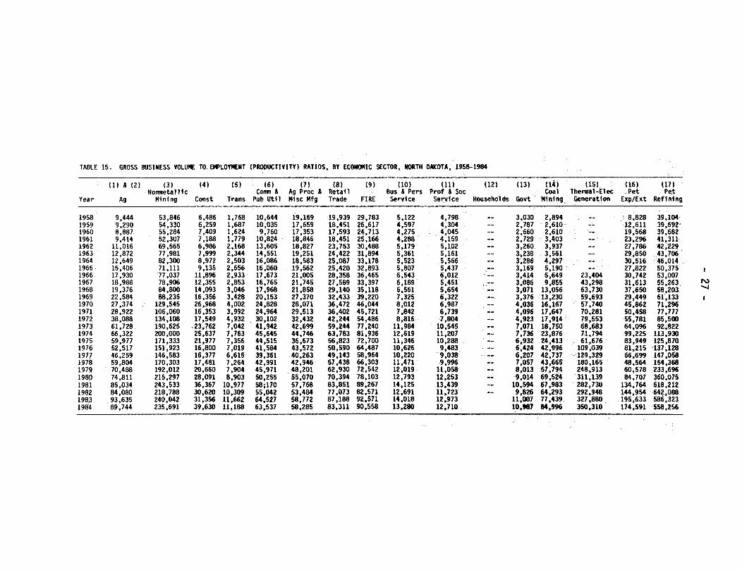
TABLE 15. GROSS BUSINESS VOLUME TO EMPLOYMENT (PRODUCTIVITY) RATIOS, BY ECONOMIC SECTOR, NORTH DAKOTA, 1958-1984

(1) & (2) (3) (4) (5) (6) (7) (8) (9) (10) (11) (12) (13) (14) (15) (16) (17)Nonmetallic Comm & Ag Proc & Retail Bus & Pers Prof & Soc Coal Thermal-Elec Pet Pet

Year Ag Mining Const Trans Pub Util Misc Mfg Trade FIRE Service Service Households Govt Mining. Generation Exp/Ext Refining

6,486 1,768 10,6446,259 1,687 10,0357,409 1,624 9,7607,188 1,779 10,8246,986 2,168 13,6057,999 2,344 14,5518,972 2,503 16,0869,135 2,656 16,060

11,896 2,933 17,67312,355 2,853 16,76514,093 3,046 17,96816,356 3,428 20,15326,968 4,002 24,82816,353 3,992 24,96417,549 4,932 30,10223,762 7,042 41,94225,637 7,763 45,64521,977 7,356 44,51516,800 7,019 41,58416,377 6,615 39,36117,481 7,264 42,99120,660 7,904 45,97128,091 8,903 50,25536,367 10,977 58;17030,620 10,309 55,04231,356 11,662 64,52739,630 11,188 63,537

19,16917,65917,35318,84618,82719,25118,58319,56221,00521,74521,85827,37028,07129,51332,43242,69944,74636,67343,57240,26342,94648,20155,07057,76853,48458,77258,285

19,939 29,78318,451 26,61717,593 24,71318,451 25,16623,753 30,48824,422 31,89425,087 33,17825,420 32,89328,358 36,46527,589 33,39729,140 35,11832,433 39,22036,472 46,04436,402 45,72142,244 54,48659,244 77,24063,783 81,93656,823 72,70050,590 64,48749,143 58,96457,438 66,30362,930 72,54270,394 78,10383,851 89,26777,073 82,57187,188 92,57183,311 90,558

5,1224,5974,2754,2885,1795,3615,5235,8076,5436,1896,5617,3258,0127,8428,816

11,98412,61911,34610,62610,22011,47112,01912,79314,12512,69114,01813,280

4,7984,3044,0454,1595,1025,1615,5665,4376,0125,4515,6546,3226,9876,7397,804

10,54511,20710,2889,4839,0389,996

11,05812 25313,43911,72312,97312,710-

3,030 2,8942,787 2,6102,660 2,6102,729 3,4033,260 3,9373,238 3,5613,286 4,2973,169 5,1903,414 5,6493,086 9,8553,071 13,0563,376 13,2304,036 16,1674,096 17,6474,923 17,9147,071 18,7507,736 23,8766,932 24,4136,424 42,9966,207 42,7377,057 43,6658,013 57,7949,014 69,524

10,594 67,9839,826 64,293

11,007 77,43910,987 84,996

--

23,40443,29863,73059,69357,74070,28179,55368,6837.1,79461,676109,039129.,329180,165248,913311,139282,730292,948327,.880350,310

8,828 39,10412,611 39,69219,568 39,68223,296 41,31127,786 42i22929,850 43,70630,516 46,01427,822 50,37530,742 53,00731,613 55,26337,650 58,20329,449 61,13345,862 71,29650,458 77,77755,781 85,50064,096 92,82299,225 113,93083,949 125,87081,215 137,12866,699 147,05848,564 154,36860,578 233,69684,707 360,075

134,764 618,212144,954 642,088195,633 586,323174,591 558,256

19581959196019611962196319641965.1966196719681969197019711972197319741975197619771978197919801981198219831984

9,4449,2908,8879,414

11,01612,87212,64915,40617,93018,98819,37622,58427,37428,92238,08861,72866,32259,97752,51746,25959,80470,48874,81185,03484,08093,63589,744

53,84654,33055,28452,30769,56577,98182,30071,11177,03778,90684,80088,235

129,545106,060134,108190,625200,000171,333151,923146,583170,303192,012215,297243,533218,788240,042235,691

I

,,

- 28 -

secondary (or indirect and induced) employment. Secondary employment is thatwhich will arise as a result of the expenditures from the development as theyare spent and respent throughout the economy by the multiplier process. Thisemployment is in addition to the workers directly employed by the new project,and essentially comes into existence to serve and supply the new development.Impact analyses typically list direct and secondary employment resulting froma development. Estimating secondary employment by using productivity ratiosprovides sector-specific secondary employment estimates, contrasting to theaggregate ratio method (which assumes the ratio to be applicable to allsectors) characteristic of export base models. It should be noted that thismethod of estimating secondary employment will not conform to classicsecondary/direct employment ratios. Because the dollar is considered theforce that is necessary to create a job, industries that are more capitalintensive (typically with greater levels of expenditure per direct job) willoften have higher secondary/direct employment ratios.

Tax Revenue Estimation

Several state tax revenues can be estimated using the input-outputmodel. These include state personal income tax, state corporate income tax,and sales and use tax collections. Tax revenue estimates are based onhistoric relationships between tax collections and input-output modelestimates of gross business volumes for selected sectors. Tax ratescalculated were based on state tax rates in existence in 1983 (Coon et al.1984). Estimates of state personal income tax collections were based on thefollowing relationship:

State personal income tax collections= 2.1 percent X personal income.

Personal income from the input-output model is the gross business volume ofthe household sector (Sector 12). The equation to estimate state corporateincome tax collections is

State corporate income tax collections = .31 percent X grossbusiness volume of all business sectors.

All business sectors consist of all sectors of the economy except for theagriculture (Sector 1 and Sector 2), households (Sector 12), and government(Sector 13) sectors. State sales and use tax collections were estimated basedon the following formula:

State sales and excise tax collections = 4.06 percent X retail trade.

Retail trade is the gross business volume of the retail trade sector (Sector

8) of the input-output model. Caution should be used when applying the taxestimator rates as they were based on tax laws as they existed in 1983. Iftax rates change, these estimators may not accurately predict tax revenues.Also, after a change in state tax rates a lag of a minimum of one year willoccur before data are available to produce new estimators. More than one

year's tax collection data should be available before new estimators are

calculated if they are to be used with a high level of confidence.

- 29 -

Tax revenue estimators currently being used have been used inconjunction with impact analysis and contribution studies. Ratios developedat the state level are assumed to apply to single projects or industries.This means that the in-state expenditures for a particular development can beapplied to the multipliers to yield levels of business activity. Applying thetax rate estimators to the business activity of the proper sectors willproduce estimates of personal income, state income, and sales and excise taxrevenues for North Dakota.

Regional Input-Output Model

The North Dakota input-output model has been used for analysis ofsubstate regions with relative accuracy (Lutovsky 1968; Senechal 1971). Eightstate planning regions have been defined with each having a major retail tradecenter (Figure 1). Each of these regions in effect is an economic system and,therefore, the multipliers can be applied to the economic base to provideestimates of business volumes. One set of interdependence coefficients wasused for economic analysis of both state and substate regions when the I-0model consisted of 13 sectors. Expansion of the model to 17 sectors(Hertsgaard et al. 1977) resulted in an unusual occurrence; the petroleumrefining sector had a large volume of exports from the producing region toother regions within North Dakota. Thus, separate technical coefficientstables were developed for the state and the state's regions. The resultantmultipliers were slightly different for the state and the regions (Coon et al.1984).

Figure 1. North Dakota State Planning Regions

- 30 -

Sales for final demand, gross business volumes, employment,productivity ratios, and model validation tables were developed for each ofNorth Dakota's eight State Planning Regions (Coon et al. 1984). These tableswill not be duplicated in this report, but it should be noted that allinput-output analysis undertaken at the state level also has been completed atthe regional level. Economic analysis using input-output at a regional levelis handled in a similar manner; regional multipliers are applied to in-regionexpenditures to estimate regional business activity. This business activitycan be divided by the region's respective productivity ratios to estimatesecondary employment at this level. Also, state tax ratios can be applied tothe proper business activity to determine estimated tax revenue collections.In essence, the methodology for input-output analysis is the same at the stateor substate level, but the corresponding input-ouput tables used to performthe analysis may differ.

A brief comparison of regional personal income estimates from theDepartment of Commerce and the I-0 model will be used to validate the model atthe substate level. Table 16 presents a comparison of each region and thestate for selected statistical tests. Income estimates vary more over time atthe region level than for North Dakota, but the Theil coefficient indicatesthis variability does not preclude use of the model at this level and in factthe closeness of the values to 0.0 would indicate the model performs quitewell and can be used with confidence.

Uses of Input-Output Analysis In North Dakota

Input-output analysis is a technique that is quite easy to use toestimate the economic impacts of new income injections into the economy. Acommon use of input-output analysis is to assess the effect of a newmanufacturing or processing plant in the state. In such a case there will bea one-time impact on the state's economy that results from the construction ofthe facility. There also will be annually recurring impacts associated withthe operation of the plant after the plant is completed and productionbegins.

Information needed to estimate the economic impacts of a new plant inthe state is the set of expenditures that will be injected into the respectivesectors of the state's economy during the construction and the operationphases of the plant. These expenditures are multiplied by the appropriateinterdependence coefficients of the input-output model to provide estimates ofgross income changes for the respective sectors in the state that areattributable to the construction and operation of the new plant. Typically,new income is injected into the state during the construction phase throughthree sectors: the contract construction sector (expenditures to firms in theconstruction industry), the retail trade sector (expenditures for materialspurchased within the state), and the household sector (payrolls of employeesnot already included as part of the expenditures to the contract constructionsector). New income is injected into the state's economy during the operatingphase of the new plant via two sectors: the retail trade sector (formaterials purchased from other firms in the state each year) and the householdsector (the new plant' s payroll after operation begins).

- 31 -

TABLE 16. COMPARISON OF STATISTICAL TESTS FOR THE INPUT-OUTPUT MODEL PERSONALINCOME ESTIMATION, NORTH DAKOTA REGIONS 1-8 AND STATE, 1958-1984

Average Absolute Mean Average Standard TheilRegion Differencea Difference Deviationc Coefficientd

1 12.64 - 5.26 15.43 0.142 8.91 3.86 10.90 0.083 20.55 19.91 11.81 0.164 9.77 7.45 11.15 0.085 18.64 -18.28 11.14 0.226 8.57 7.58 6.62 0.077 5.80 - 5.56 6.19 0.108 14.68 13.56 11.22 0.13

STATE 5.47 - 1.88 6.27 0.07

aAverage absolute difference is the sum of the absolute values of the percentdifference of I-0 estimates and historic data divided by the number ofobservations.

bMean average difference is the sum of the percent difference of the I-0estimate and historic data divided by the number of observations.

cStandard deviation is for the difference of the I-0 estimate and historicdata.

dTheil's coefficient is calculated using the formula:

T E(Ys - Ya) 2

U1 =

ST E(Ys)2 + T (Ya)2

where: T = time periodYs = simulated value of YYa = actual value of Y

Input-output anlaysis also has been used to measure the impact of anexisting industry or plant in a fully operational stage. This type ofinput-output analysis is termed a contribution study (i.e., I-0 methodology isused to measure the business activity, employment, personal income, and taxrevenues an industry contributes to the current economy of the state). Thistype of study provides estimates of the absolute size of an individual firm orindustry and their relative importance to the state economy. Also,input-output analysis can be used for analyses, such as revenue forecastingand analyzing the state's economic base and its composition.

The input-output model also has been incorporated as one module of alarge economic-demographic assesment model for simulating the North Dakotaeconomy. In this model, the input-output interdependence coefficients are

- 32 -

applied to forecasts of future sales to final demand (exports) for eachrelevant sector to develop estimates of gross business volume for all sectorsof a given substate region. The projected levels of gross business volumethen are used to estimate employment in each sector. These employment levelsthen provide a basis for estimating the extent of net in- or out-migration andhence the likely extent of population growth or decline in the region.Input-output analysis serves as the driving mechanism of this comprehensivesocioeconomic assessment model.

Examples of Input-Output Analysis

A number of studies in North Dakota have employed input-output analysisto estimate the economic impacts of various types of developments. The topicsaddressed in these studies have covered a wide range of issues involving NorthDakota. Studies involved with irrigation, coal or other energy development,feasibility, contribution, recreation, government programs, and comprehensivesocioeconomic model development have relied heavily on the North Dakota I-0model's economic estimates. Not all studies completed in each of these areaswill be referenced, but rather a few selected reports associated with eachtopic will be noted.

The North Dakota I-0 model was developed principally to analyze theeconomic impacts associated with irrigation development in the state(Schaffner and Carkner 1975; Leitch and Anderson 1978); this probably was thelargest proposed single resource development project in the state up to thattime. The model was used for analyzing other agricultural impacts such asthose occurring from added growing-season rainfall (Schaffner et al. 1983).

Feasibility studies almost always include an analysis of the economicimpact associated with the particular project development. This analysis isimportant because it indicates how the development will help the state'seconomy in terms of personal income and employment. Often, when state fundingis being sought, the economic impact has a bearing on securing state loans,etc. Feasibility studies have primarily focused on processing of the state'sagricultural products and have included projects such as malt plants (Andersonand Frasse 1970), wheat gluten plants (Mittleider et al. 1978), pastaprocessing (Fraase, Walsh, and Anderson 1974; Mittleider and Anderson 1978),and sunflower processing plants (Cobia et al. 1977). For a complete listingof economic impacts associated with feasibility studies done in North Dakota,see Mittleider et al. (1983b). Input-output analysis also has been used toanalyze the economic impacts associated with rural industrialization (Helgesonand Zink 1973).

Large-scale energy development in western North Dakota brought with itan increased need for analyzing economic impacts. The North Dakota I-0 modelwas used extensively for estimating impacts with coal development projects inthe 1970s. Impact assessments were provided for such projects as a coalgasification plant (Dalsted et al. 1976) and coal mine development (Toman etal. 1977). The North Dakota input-output model provided the basis for a verycomprehensive socioeconomic impact assessment model with the acronym NEDAM.This computer model was developed in the 1970s and became fully operationalwith documentation a short time later (Leistritz et al. 1982). NEDAM became

- 33 -

so popular and well-reviewed throughout the United States that it subsequentlywas adopted for usuage in Wyoming (Coon et al. 1983), Montana (Chase et al.1982), and Minnesota (Coon, Vocke, and Leistritz 1984a). These models can beused to analyze the socioeconomic impacts associated with a development of anytype in the respective states. NEDAM continues to be used extensively andconstantly is being updated and enhanced as data become available (Coon et al.1984).

Economic impacts associated with North Dakota recreation have beenanalyzed using the I-0 model. Studies involving recreation development(Helgeson and Holte 1978; Mittleider and Leitch 1984a), nonresident sportsmenexpenditures (Anderson and Leitch 1984), and the contribution of state parksto the North Dakota economy (Mittleider and Leitch 1984b) have been analyzed.

Composition of the North Dakota economy and how it is changing havebeen analyzed using input-output analysis (Coon, Vocke, and Leistritz 1984b).The model also has been used in such diverse projects as economic contributionstudies (Coon, Mittleider, and Leistritz 1983), transportation models(Mittleider, Tolliver, and Vreugdenhil 1983), and for analyzing impacts of thePayment in Kind (Federal Government Agricultural Program) on the North Dakotaeconomy (Mittleider et al. 1983a).

As can be discerned from its extensive applications, the North Dakotainput-output model is a useful and accurate tool for describing the economiclinkages and interrelationships of North Dakota's economy. This model hasbeen used to determine the effects of a wide variety of industrial andagricultural developments in North Dakota. Analyzing the impacts from thesedevelopments using input-output analysis has proven to be accurate andbeneficial to both private industry and government personnel. The value ofhaving economic information, such as that provided by input-output analysis,has become more apparent in recent years with the much larger developments(e.g., the coal gasification plant in western North Dakota). The better theeconomic impact assessment information available to policymakers, the moreeffectively the impacts associated with a development can be managed.

Interpreting the Results of An Economic Impact Assessment

An example of an actual economic impact assessment will be presented inorder to further explain the results of such an analysis. Excerpts from ananalysis of the contribution of state parks (Mittleider and Leitch 1984b, p.7ff.) will show the type of information required and the interpretation of theresults. (The tables associated with the excerpts are numbered as they werein the original publication and are presented following the excerpts.)

State park operation-and-maintenance expenditures occurred inseveral sectors of the economy (Table 5). Households (wages and

salaries), construction, and retail trade were the sectors withthe largest state park expenditures, accounting for over 90percent of the total. State park operation-and-maintenanceexpenditures totaled $2,753,448 in fiscal 1984, compared to the

previous five-year average of $2,102,529. Headquarteroperations accounted for over 38 percent of total parkexpenditures.

- 34 -

Applying state park operation-and-maintenance expenditures tothe interdependence coefficients yielded total business activityfor all sectors. Personal income, retail sales, businessactivity for all business sectors, and total business activitywere estimated for each state park for fiscal 1984 (Table 6).These values include both the first-round effect (Table 5) andthe secondary impact. Operation-and-maintenance expenditures bythe state park system resulted in personal income of over $2.6million and retail sales over $2 million. Over $7 million intotal business activity occurred as a result of the original$2,753,448 in state park operation-and-maintenance expenditures.The multiplier effect for these expenditures was 2.65, meaningthat each dollar spent for state park operation and maintenancegenerated $2.65--the original dollar plus $1.65 in additionalbusiness activity.

Personal income, retail sales, and business activity of allbusiness sectors were used to estimate income tax collectionsresulting from state park operation-and-maintenance expenditures(Table 7). Personal income tax estimates included both directand secondary effects; that is, income taxes attributable towages and salaries for state park employees plus income taxesresulting from the multiplier effect. Total tax collectionsaccruing to the state were $86,978 as a result of state parkoperation-and-maintenance expenditures. Sales and use taxcollections of over $50,000 (58 percent of the total) were thelargest tax collection category, followed by personal incometaxes of $23,700 (27 percent) and corporate income taxes of$13,000 (15 percent).

In addition to tax revenues, operation-and-maintenanceexpenditures create direct and secondary employmentopportunities. Direct employment figures were obtained from theNorth Dakota Parks and Recreation Department, and secondaryemployment was estimated by using productivity ratios, thenumber of dollars of business activity, needed to support oneworker for each respective sector. Direct employment in stateparks, in full-time equivalents, was 68.5 for fiscal 1984 (Table8). Secondary employment, resulting from additional rounds ofspending, was estimated to be 106 people for the same period.

TABLE 5. ESTIMATED NORTH DAKOTA STATE PARK OPERATION-AND-MAINTENANCE EXPENDITURES, BY ECONOMIC SECTOR ANDPARK, FISCAL YEAR 1984

Expenditures by SectorFinance, Business &

Communication & Retail Insurance, PersonalState Park Construction Transportation Public Utilities Trade Real Estate Service Household Total

- - - -- - -- - - - - - - - ---- - - - - - -dollars- - - - - - - - - - - - - - - -- - - - -

Beaver Lake,Doyle, &Streeter

Fort Lincoln,Butte View, &Sully Creek

Fort Stevenson

Fort Ransom

Icelandic

Lake Metigoshe

Lake Sakakawea& LittleMissouri Bay

Lewis & Clark

Turtle River &Devils Lake

Headquarters

Total

540

147,000

215,000

35,000

30,000

45,000

152,417

36,200

116,500

777,117

945

900

540.

990

990

990

990

1,035

20,460

28,380

2,926

14,715

9,237

3,263

8,798

13,388

12,634

7,729

11,475

18,926

103,041

11,394

28,120

19,405

10,891

19,283

27,647

26,832

17,283

1,260

2,498

1,620

1,215

2,295

1,845

3,060

1,575

27,317 3,060

447,337 1,755

635,509 20,183

664

1,745

1,166

754

1,166

1,919

1,745

1,166

1,919

101,718

113,962

36,368 53,152

102,983

83,101

28,246

83,968

101,460

103,533

77,221

113,070

345,256

1,075,206

298,006

330,429

44,909

151,500

177,249

193,794

258,381

194,076

1,051,952

2,753,448

I

(A)(-7,I

- 36 -

TABLE 6. ESTIMATED PERSONAL INCOME, RETAIL SALES, BUSINESS ACTIVITY OFALL BUSINESS (NONAGRICULTURAL) SECTORS, AND TOTAL BUSINESS ACTIVITY,RESULTING FROM STATE PARK SYSTEM OPERATION-AND-MAINTENANCE EXPENDITURES,BY PARK, FISCAL YEAR 1984

BusinessPersonal Retail Activity of All Total Business

State Park Income Sales Business Sectorsa Activity-- - - - - - - - -- -- -dollars- --- - - - - ---

Beaver Lake,Doyle, &Streeter

Fort Lincoln,Butte View, &Sully Creek

Fort Stevenson

Fort Ransom

Icelandic

Lake Metigoshe

Lake Sakakawea& LittleMissouri Bay

Lewis & Clark

Turtle River &Devils Lake

Headquarters

Total

65,794

277,418

278,583

53,261

170,811

201,942

214,702

229,310

223,583

893,469

2,608,873

44,303

182,118

180,850

37,772

107,856

131,501

138,575

147,477

142,289

941,102

2,053,843

76,052

472,027

537,121

65,219

226,771

262,841

291,403

414,847

287,781

1,609,220

4,243,282

151,981

792,684

859,196

126,949

423,403

495,686

538,903

679,679

545,149

2,678,768

7,292,398

alncludes all sectors exceptand government.

agriculture (crops and livestock), households,

- --

- 37

TABLE 7. ESTIMATED TAX REVENUES RESULTING FROM NORTH DAKOTA STATE PARKOPERATION-AND-MAINTENANCE EXPENDITURES, FISCAL YEAR 1984

Sales and Personal CorporateState Park Use Taxa Income Tax Income Tax Total

Beaver Lake,Doyle, &Streeter 1,165 599 233 1,997

Fort Lincoln,Butte View, &Sully Creek 5,452 2,525- 1,449 9,426

Fort Stevenson 5,715 2,535 1,649 9,899

Fort Ransom 952 485 200 1,637

Icelandic 3,135 1,554 696 5,385

Lake Metigoshe 3,676 1,838 807 6,321

Lake Sakakawea& Little.Missouri Bay 3,956 1,954 895 6,805

Lewis & Clark 4,609 2,087 1,274 7,970

Turtle River &Devils Lake 4,070 2,035 883 6,988

Headquarters 17,479 8,131 4,940 30,550

Total 50,209 23,743 13,026 86,978

aIncludes only tax assessments on nonpark expenditures to the retail tradesector as parks do not pay sales and use tax. Taxable retail sales aretotal retail sales (Table 6) less park operation-and-maintenanceexpenditures to the retail trade sector (Table 5).

- 38 -

TABLE 8. ESTIMATED DIRECT AND SECONDARY EMPLOYMENT ATTRIBUTABLE TO NORTHDAKOTA STATE PARK OPERATION-AND-MAINTENANCE EXPENDITURES, FISCAL YEAR 1984

State Park Direct Employmenta Secondary Employment

Beaver Lake,Doyle, &Streeter 3.75

Fort Lincoln,Butte View, &Sully Creek 7.00 12

Fort Stevenson 6.25 14

Fort Ransom 2.75

Icelandic 6.25 4

Lake Metigoshe 6.50 4

Lake Sakakawea& LittleMissouri Bay 6.50 6

Lewis & Clark 4.50 11

Turtle River &Devils Lake 7.50 5

Headquarters 17.50 50

Total 68.50 106

aIncludes part-time employees. Part-time personnel are reported infull-time equivalents. Obtained from the North Dakota Parks and RecreationDepartment.

- 39 -

Summary

The purpose of this report was to provide a reference and companiondocument to accompany input-output related presentations and reports.Input-output theory, the history of the North Dakota I-0 model, North DakotaI-0 data tables, applications of the model, and an actual impact assessmentwere included to cover the subject completely. This document will primarilybe used as a reference for persons interested in input-output analysis and howit relates to the North Dakota economy.

As can be seen from the section on examples of the model's useage, theNorth Dakota input-output model has become an integral part of state-orientedeconomic research. Primary benefits from I-0 analysis have been to help planfor the socioeconomic impacts associated with a particular development.However, planners and decision makers of all kinds have benefited from theestimates provided by the model. Development of the NEDAM model furtherhighlights the usage of the input-output model for forecasting purposes of notonly economic but also socioeconomic variables.

The North Dakota input-output model has evolved in scope from theinterdependency of a local community to a state and substate economic tool ina period of approximately 20 years. During this period the model has gonethrough several revisions to arrive at the current version. Importance andflexibility of the I-0 model are further exemplified by the fact that it hasundergone upgrades and enhancements and can easily be expanded to betterdescribe additional state industrial sectors. Economic researchers have usedthe North Dakota input-output model extensively and will continue to rely onit in the future because of its ability to provide an accurate and detailedeconomic analysis.

Appendix A

Definition of Terminology

- 43 -

Terms

Basic Economic Activity: an economic activity that produces output for finaldemand (which, in North Dakota, is principally for export from the area).

Business Activity: computationally, the resultant of the application of themultipliers to the expenditures within an area by a firm or industry.This term is used when analyzing a firm or industry's expenditures for animpact or contribution study.

Constant (Base Year) Dollars: dollars expressed in terms of purchasing powerfor a base year's prices.

Contribution Study: an economic study in which the expenditures of anindividual firm or industry in an area are used to measure its relativemagnitude to the economic unit.

Current (Year) Dollars: dollars reflecting their purchasing power in terms ofthat given year's prices.

Direct Employment: workers employed by a firm or industry being analyzed by animpact or contribution study.

Economic Base: those economic activities within an area which produce productsexported from that area in return for dollars.

Economic Impacts: resultant increase or decrease in economic activityresulting from the expansion or shrinkage of a particular firm, industry,or sector in the area economy.

Economic Sector: a grouping of firms engaged in similar types of economicactivities.

Gross Business Volume: computationally, the resultant of the application ofthe multipliers to the sales for final demand. These values indicate thetotal dollar volume of business activity occurring after ,the multiplierprocess has been completed.

Gross Receipts Multiplier: total output requirements of all row sectors in theeconomy per dollar of output for final demand by the column sector.

Identity Matrix: a matrix consisting of all zeros except for one's in the main(upper left to lower right) diagonal.

Input-Output Analysis: a technique for tabulating and describing the linkagesor interdependencies between various industrial groups within an economy.

Interdependence Coefficients (Multipliers): computationally, they are theinverse of the [I-A] matrix, or [I-A]- 1 . Each element of the matrix showsthe total (direct and indirect) input requirements that must be obtainedfrom the row sector per dollar of output for final demand by the columnsector.

- 44 -

Personal Income: gross business volume of the household sector of theinput-output model.

Productivity Ratio: the ratio of gross business volume to employment. Thesevalues indicate the amount of business activity necessary to maintain orcreate one job in each sector of the economy.

Retail Trade Center: a city with retail trade activities serving itself andthe surrounding trade area.

Sales for Final Demand (Final Demand Vector): the value (measured in terms ofdollars) of exports from the economic unit by a basic economic sector.

Secondary (Indirect and Induced) Employment: workers not employed directly bythe firm or industry being analyzed by a contribution or impact study, butwhose jobs were created as the result of expenditures by the particularfirm or industry.

Technical Coefficients: the transactions table expressed as decimal fractionsof column totals in the transactions table. This table is usuallyreferred to as the A matrix.

Transactions Table: a table showing the purchases and sales by each of theeconomic sectors to each of the sectors. Columns show purchases from (andpayments to) each row sector, and the rows indicate the sales of that rowsector to the column sectors.

Appendix B

North Dakota Input-Output Tables in Constant Dollars

APPENDIX TABLE 1. SALES FOR FINAL DEMAND, BY ECONOMIC SECTOR, NORTH DAKOTA, MILLION DOLLARS, (1980=BASEDOLLARS), 1958-1984

(1) (2) (4) (7) (8) (10) (12) (14) (15) (16) (17)Ag, Ag, Ag Proc & Retail Bus & Coal Thermal- Pet Pet

Year Lvstk Crops Constr Misc Mfg Trade Pers Serv Householdsa Mining Elec Gen Exp/Ext Refining Total

195819591960196119621963196419651966196719681969197019711972197319741975197619771978197919801981198219831984

591.7570.0452.8547.1500.6513.6520.0590.0627.2630.1567.7541.4528.3563.0667.4798.4691.9639.5650.1612.8625.6756.1781.4538.9517.6545.8524.1

1,182.61,035.91,009.0

873.91,197.71,343.01,100.01,321.81,407.71,275.01,225.81,311.11,300.91,244.81,728.73,012.43,196.72,197.51,603.11,494.41,908.81,843.81,721.62,122.41,974.32,147.41,874.6

49.271.484.461.441.442.373.673.953.854.758.071.9

353.0112.2129.3103.3111.7117.160.365.677.885.0

108.171.548.065.688.6

167.9149.5170.6172.6157.2180.5191.1186.9194.5205.7218.1330.9287.1299.3301.4407.6470.2433.1627.1517.4515.0570.6562.2559.1450.8442.3454.5

44.347.2.38.544.047.053.763.978.7

104.0122.7149.8154. 9166.1173.3153.0158.5142.9158.9180.1182.1195.0160.7144.5145.5143.2161.8140.4

14.815.712.914.815.817.821.226.234.740.849.851.755.357.851.152.848.053.060.160.664.953.648.248.547.754.046.8

502.3489.2485.0606.6864.6827.2

1,182.8861.5990.1854.2962.4

1,024.51,100.61,118.11,150.71,219.11,243.41,478.71,431.81,365.21,368.21,505.31,687.41,720.51,368.31,595.01,692.4

3.02.62.63.3,3.83.23.73.63.04.75.24.96.26.5,5.96.97.6

10.021.523.126.035.148.349.449.563.276.5

--

10.218.826.423.926.832.337.932.434.629. 151.858.777.399.8

120.1127.7138.7161.8179.7

14.528.637.453.757.357.663.166.768.662.873.753.558.760.861.364.4

117.4119.1135.3129.3128.2198.8410.4882.8734.0644.8571.5

35.233.832.332.231.430.9131.031.932.332.831.630.429.529.429.832.034.935.336.237.036.451.174.3

119.6103.992.986.9

2,605.52,443.92,325.52,409.62,916.83,069.83,250.43,241.23,526.13,302.33,368.53,599.13,912.53,697.54,316.55,887.86,099.35,271.34,857.44,546.25,023.25,359.95,706.56,385.95,576.05,974.65,736.0

aHousehold sector sales for final demandand Leistritz (1986).

include oil lease bonus payments as estimated by Coon, Anderson,

I

-p^,

APPENDIX TABLE 2. GROSS BUSINESS VOLUMES OF ECONOMIC SECTORS ESTIMATED BY THE INPUT-OUTPUT MODEL, NORTH DAKOTAMILLION DOLLARS, (1980=BASE DOLLARS), 1958-1984

(1) (2) (3)Ag, Ag. Nonmetallic

Year Lvstk Crops Mining

(4) (5) (6) (7) (8) (9) (10) (11) (12) (13) (14) (15) (16) (17)Comm & Ag Proc & Retail Bus:& Pers Prof & Soc House- Coal Thermal-Elec Pet Pet

Const Trans Pub Util Misc Mfg Trade FIRE Service Service holds Govt Mining Generation Exp/Ext Refining

1958 878.8 1,649.51959 838.1 1,468.91960 698.0 1,406.91961 810.0 1,301.01962 793.1 1,633.11963 822.6 1,811.21964 839.7 1,565.51965 920.5 1,824.61966 984.4 1,942.41967 972.7 1,803.31968 906.5 1,737.31969 907.6 1,895.11970 898.9 1,856.71971 932.5 1,814.71972 1,097.2 2,386.21973 1,379.3 3,910.21974 1,278.3 4,110.71975 1,148.2 2,981.61976 1,150.4 2,462.51977 1,072.0 2,256.51978 1,121.6 2,713.91979 1,293.0 2,734.41980 1,328,6 2,612.51981 1,075.6 2,956.61982 990.8 2,705.81983 1,053.9 2,907.91984 1,013.8 2,611.9

18.718.117.517.420.021.122.622.924.122.622.724.533.125.930.740.842.236.331.829.933.335.637.739.834.537.436.3

251.4 31.2260.8 29.3265.2 27.6250.4 28.8274.6 33.9286.4 35.7334.4 37.1329.4 37.9331.8 41.0311.5 38.7320.0 39.0349.8 41.4648.6 44.4396.9 42.3463.1 49.6560.6 67.9588.1 70.3530.6 60.3436.7 56.0418.0 52.2466.0 57.5502.5 62.0561.7 67.0599.2 77.1504.5 67.3549.8 70.5551.5 66.9

228.7213.8202.4212.7260.8272.6294.3286.6312.9290.5296.5316.5337.5325.2378.3512.1527.2462.6424.8397.4436.1464.5488.7527.5458.2498.1481.5

846.8 1,949.6 405.6 171.7778.9 1,809.4 375.6 160.5743.8 1,708.8 355.9 150.3784.6 1,759.1 367.6 155.5793.9 2,169.0 454.9 190.5864.1 2,292.2 478.7 202.3863.2 2,399.1 503.9 212.9919.2 2,409.0 498.8 217.9974.6 2,635.9 543.2 243.1970.4 2,464.3 502.6 233.5955.1 2,512.0 508.7 244.2

1,152.8 2,686.4 544.9 260.21,077.3 2,831.9 573.3 273.41,106.0 2,744.6 554.9 269.21,248.5 3,216.7 657.8 303.41,717.6 4,466.0 916.7 409.31,796.3 4,589.3 945.4 416.31,551.2 3,917.4 806.1 363.11,799.7 3,545.1 726.9 337.41,567.9 3,319.9 678.4 319.11,640.6 3,695.1 754.3 353.71,808.8 3,848.9 797.3 357.31,800.8 3,937.0 822.6 359.71,727.4 4,197.1 875.7 381.91,486.9 3,692.8 766.7 340.11,528.7 4,043.3 839.7 373.81,498.3 3,860.0 808.3 352.7

181.4169.4160.3170.1211.5219.7241.8230.0251.9231.9237.3253.3268.9261.0302.8406.1417.1371.2339.6318.1347.6370.7388.5409.8354.3390.0380.7

2,746.3 246.2 3.02,566.5 228.8 2.62,432.8 216.2 2.62,586.7 225.5 3.33,229.7 277.8 3.83,347.9 291.3 3.23,708.4 310.4 3.73,504.5 304.6 3.63,840.2 332.1 4.63,528.5 307.4 7.73,619.4 311.8 9.43,863.0 333.4 8.74,104.9 351.5 10,53,984.9 340.7 11.64,612.5 400.8 11.96,164.6 551.4 12.16,332.4 567.3 13.15,663.7 490.2 14.65,182.5 445.2 29.74,855.6 415.9 32.45,295.8 459.3 38.35,650.6 487.2 51.05,930.5 505.3 67.46,259.2 536.1 69.95,398.5 467.7 71.75,949.4 511.9 89.05,815.4 494.2 105.1

10.218.826.423.926.832.337.932.434.629.151.858.777.399.8

120.1127.7138.7161.8179.7

45. 35.45.2 35.359.4 33.867.8 32.385.7 32.389.0 31.588.9 31.095.0 31.199.7 32.0

102.2 32.596.3 33.1

107.4 32.084.2 30.789.2 29.991.5 29.892.4 30.397.6 32.4158.2 35.4160.4 35.8179.3 37.1173.4 38.0171.9 37.6261.9 52.7513.8 76.3

1,070.2 121.7893.9 106.1787.2 95.6702.1 90.0

00IOo

APPENDIX TABLE 3. GROSS BUSINESS VOLUME TO EMPLOYMENT (PRODUCTIVITY) RATIOS, BY ECONOMIC SECTOR, NORTH DAKOTA, (1980=BASE DOLLARS), 1958-1984

(1) & (2) (3) (4) (5) (6) (7) (8) (9) (10) (11) (12) (13) (14) (15) (16) (17)Nonmetallic Comm & Ag Proc & Retail Bus & Pers Prof & Soc House- Coal Thermal-Elec Pet Pet

Year Ag Mining Const Trans Pub Util Misc Mfg Trade FIRE Service Service holds Govt Mining Generation Exp/Ext Refining

143,846 17,422 4,757 28,605142,519 16,424 4,414 26,326142,276 19,134 4,191 25,199133,846 18,386 4,534 27,673173,913 17,553 5,445 34,185193,577 19,784 5,811 35,996200,000 21,869 6,111 39,224169,629 21,774 6,331 38,295178,518 27,487 6,795 40,811176,562 27,708 6,421 37,610181,600 30,288 6,564 38,606180,147 33,419 6,992 41,178250,758 52,277 7,761 48,132196,212 30,216 7,374 46,127237,984 31,113 8,737 53,364318,750 39,860 11,806 70,353308,029 39,552 11,967 70,424242,000 31,038 10,389 62,878203,846 22,553 9,426 55,813185,714 20,770 8,381 49,912201,818 20,660 8,594 50,809209,165 22,508 8,610 50,078215,297 28,091 8,903 50,255220,933 32,993 9,958 52,772187,326 26,219 8,827 47,126197,698 25,824 9,606 53,148187,119 31,463 8,882 50,444

51,48346,33044,78548,19747,28647,59845,30046,63348,52348,77846,96855,91554,42054,53157,50071,62969,03051,80158,48451,05050,75152,50855,07052,40745,79448,40746,273

53,560 80,00048,399 69,81445,414 63,78147,189 64,37859,666 76,58260,397 78,86361,160 80,88260,596 78,42765,512 84,21761,887 74,90362,613 75,47466,258 80,13270,711 89,27167,261 84,485/4,902 96,60799,385 129,58798,400 126,40780,259 102,68767,907 86,56662,311 74,75467,878 78,35268,552 79,02270,394 78,10376,069 80,98365,990 70,69671,813 76,24766,143 71,896

13,76412,05611,04010,96813,01713,25913,47113,84615,12113,88314,09114,96015,53614,48915,63420,10419,46516,03014,26112,96313,55613,09312,79312,81310,86611,54810,545

12,89511,28610,44210,64012,81712,77013,56812,96013,89412,22712,14312,91613,54612,45813,83617,68917,29414,53212,72911,45911,81412,04612,25312,19210,03710,68610,091

8,136 7,8947,314 6,7886,863 6,7886,979 8,6388,189 9,9738,009 8,7678,012 10,6017,554 12,4567,892 12,9946,920 22,3186,600 27,8936,898 26,7697,825 31,4377,567 32,4928,726 31,818

11,862 31,51011,936 36,7979,793 34,2728,622 57,7827,870 54,0908,338 51,6178,729 62,9899,014 69,5709,611 61,6328,413 55,0569,066 63,8068,652 67,513

54,25596,907

136,787121,938112,134129,718140,892115,302110,89787,125

146,327163,966212,947271,195311,139256,425250,814270,1172781J73

23,751 105,37333,000 104,00050,446 102,53959,596 105,90169,858 106,41873,714 108,39174,334 112,68166,201 120,30070,922 122,18070,965 124,43680,873 125,00060,185 124,29188,933 138,42693,272 143,96198,929 151,500107,488 155,023153,146 176,119118,639 178,109108,996 183,66384,544 186,27457,376 182,52465,991 254,62884,707 360,075122,261 560,982124,111 549,985161,142 482,889138,609 443,438

195819591960196119621963196419651966196719681969197019711972197319741975197619771978197919801981198219831984

25,36624,36822,94124,07827,67431,82830,83536,72341,42042,59641,63446,13453,07253,43767,533

103,553102,31684,71370,49558,65170,67476,78574,81177,14471,26577,12171,273

-- I' ·

I

-II

- 51 -

References

Anderson, D.E., and R.G. Fraase. 1970. An Analysis of the Feasibility ofEstablishing Malt Plants in North Dakota. Bulletin No. 487, EconomicDevelopment Administration. Fargo: North Dakota State University,Department of Agricultural Economics.

Anderson, Randall S., and Jay A. Leitch. 1984. Characteristics andExpenditures of Nonresident Sportsmen in North Dakota in 1983.Agricultural Economics Misc. Report No. 77. Fargo: North Dakota StateUniversity, Department of Agricultural Economics.

Bartch, Bruce L. 1967. "Analysis of Intersectoral and IntercommunityStructure in Southwestern North Dakota." Unpublished M.S. Thesis.Fargo: North Dakota State University, Department of AgriculturalEconomics.

Chase, Robert A., Randal C. Coon, Connie L. Chase, Carlena F. Vocke, RebeccaJ. Vuchetich, F. Larry Leistritz, Thor A. Hertsgaard, WilliamRansom-Nelson, Steve H. Murdock, Pai-Sung Yang, and Rakesh Sharma.1982. Expansion and Adaptation of the North Dakota EconomicDemographic Assessment Model (NEDAMT for Montana: TechnicalDescription. Agricultural Economics Misc. Report No. 61. Fargo:North Dakota State University, Department of Agricultural Economics.

Cobia, David W., Delmer L. Helgeson, Randal C. Coon, Wallace C. Hardie, LeRoyW. Schaffner, and Donald F. Scott. 1977. The Economic Feasibility ofEstablishing Oil Sunflower Processing Plants in North Dakota. Bulletin503, Economic Development Administration. Fargo: North Dakota StateUniversity, Department of Agricultural Economics.

Coon, Randal C., Craig Anderson, and F. Larry Leistritz. 1986. A Methodologyfor Estimating Oil Lease Bonus Payments In North Dakota, 1979 to 1983.AE86001 Staff Paper Series. Fargo: North Dakota State University,Department of Agricultural Economics.

Coon, R.C., J.F. Mittleider, and F.L. Leistritz. 1983. Economic Analysis ofthe North Dakota Lignite Industry. Agricultural Economics Misc.Report No. 67. Fargo: North Dakota State University, Department ofAgricultural Economics.

Coon, Randal C., Carlena F. Vocke, Robert A. Chase, Brenda L. Ekstrom, WilliamRansom-Nelson, Richard W. Rathge, Thor A. Hertsgaard, F. LarryLeistritz, Rebecca J. Vuchetich, and Babu Ranganathan. 1983. Expansionand Adaptation of the North Dakota Economic-Demographic AssessmentModel (NEDAM) for Wyoming Technical Description. AgriculturalEconomics Misc. Report No. 63. Fargo: North Dakota State University,Department of Agricultural Economics.

Coon, Randal C., Carlena F. Vocke, and F. Larry Leistritz. 1984a. Expansionand Adaptation of the North Dakota Economic-Demographic AssessmentModel (NEDAM) for Minnesota: Technical Description. AgriculturalEconomics Misc. Report No. 76. Fargo: North Dakota State University,Department of Agricultural Economics.

- 52 -

Coon, Randal C., Carlena F. Vocke, and F. Larry Leistritz. 1984b. "ChangingComposition of North Dakota's Economic Base." North Dakota FarmResearch Bimonthly 42(1):7-11. Fargo: North Dakota State University,North Dakota Agricultural Experiment Station.

Coon, Randal C., Carlena F. Vocke, William Ransom-Nelson, and F. LarryLeistritz. 1984. North Dakota Economic-Demographic Assessment Model(NEDAM): Technical Description of Update and Enhancement.Agricultural Economics Misc. Report No. 75. Fargo: North Dakota StateUniversity, Department of Agricultural Economics.

Dalsted, Norman L., Arlen G. Leholm, Norman E. Toman, Randal C. Coon, Thor A.Hertsgaard, and F. Larry Leistritz. 1976. Economic Impacts of aProposed Coal Gasification Plant in Dunn County, North Dakota. Reportto Natural Gas Pipeline Company of America, Chicago, Illinois. Fargo:North Dakota State University, Department of Agricultural Economics.

Fraase, Ronald G., David E. Walsh, and Donald E. Anderson. 1974. An Analysisof the Economic Feasibility of Processing Pasta Products In NorthDakota. Bulletin 496, Economic Development Administration. Fargo:North Dakota State University, Department of Agricultural Economics.

Harmston, Floyd K., and Richard E. Lund. 1967. Application of AnInput-Output Framework To a Community Economic System. UniTversity ofMissouri Studies Volume XLII. Columbia: University of MissouriPress.

Helgeson, Delmer L., and Glen J. Holte. 1978. A Socioeconomic ImpactAnalysis of Recreation at Lake Metigoshe, North Dakota. AgriculturalEconomics Report No. 93. Fargo: North Dakota State University,Department of Agricultural Economics.

Helgeson, Delmer L., and Maurice J. Zink. 1973. A Case Study of RuralIndustrialization in Jamestown, North Dakota. Agricultural EconomicsReport No. 95. Fargo: North Dakota State University, Department ofAgricultural Economics.

Hertsgaard, Thor A., Randal C. Coon, F. Larry Leistritz, and Norman L.Dalsted. 1977. Developing Economic Impact Projection Models for theFort Union Coal Region. Project 68-01-3507, Report No. 77030. NorthDakota State University, Department of Agricultural Economics. Denver,Colorado: Environmental Protection Agency.

Leistritz, F.L., W. Ransom-Nelson, R.W. Rathge, R.C. Coon, R.A. Chase, T.A.Hertsgaard, S.H. Murdock, N.E. Toman, R. Sharma, and P.S. Yang. 1982.North Dakota Economic-Demographic Assessment Model (NEDAM): TechnicalDescription. Agricultural Economics Report No. 158. Fargo: NorthDakota State University, Department of Agricultural Economics.

Leitch, J.A., and D.E. Anderson. 1978. Impact of Inundation and Changes inGarrison Diversion Project Plans on the North Dakota Economy.Agricultural Economics Report No. 127. Fargo: North Dakota StateUniversity, Department of Agricultural Economics.

- 53 -

Leontief, Wassily. 1966. Input-Output Economics. New York: OxfordUniversity Press.

Leuthold, Raymond M. 1975. "On the Use of Theil's Inequality Coefficients."American Journal of Agricultural Economics 57(2):344-346.

Lutovsky, Richard J. 1968. "Interindustry Analysis of the North DakotaEconomy." Unpublished M.S. Thesis. Fargo: North Dakota StateUniversity, Department of Agricultural Economics.

Miernyk, William H. 1967. The Elements of Input-Output Analysis. New York:Random House.

Miernyk, William H. 1982. Regional Analysis and Regional Policy. Cambridge,Massachusetts: Oelgeschlager, Gunn, and Hain, Publishers.

Mittleider, John F., and Donald E. Anderson. 1978. Update of ... an Analysisof the Economic Feasibility of Processing Pasta Products In NorthDakota. Agricultural Economics Report No. 134. Fargo: North DakotaState University, Department of Agricultural Economics.

Mittleider, J.F., D.E. Anderson, C.E. McDonald, and Neal Fisher. 1978. AnAnalysis of the Economic Feasibility of Establishing Wheat GlutenProcessing Plants in North Dakota. Bulletin No. 508. Fargo: NorthDakota State University, North Dakota Agricultural Experiment Stationand U.S. Department of Commerce, Economic Development AdministrationCooperating.

Mittleider, John F., Randal C. Coon, Norbert A. Dorow, Tommy L. Reff, Roger G.Johnson, Thor A. Hertsgaard, LeRoy W. Schaffner, and Donald F. Scott.1983a. Economic Impact of the Payment-In-Kind Program on the NorthDakota Economy. Report prepared for the North Dakota Department ofAgriculture. Fargo: North Dakota State University, Department ofAgricultural Economics.

Mittleider, John F., Randal C. Coon, Thor A. Hertsgaard, Delmer L. Helgeson,and Eddie V. Dunn. 1983b. "Feasibility Studies Have High Payoff inNorth Dakota." North Dakota Farm Research Bimonthly 41(2):40-43.Fargo: North Dakota State University, North Dakota AgriculturalExperiment Station.

Mittleider, John F., and Jay A. Leitch. 1984a. Anchorage Marine--EconomicImpact of Recreational Development. AE84012 Staff Paper Series.Fargo: North Dakota State University, Department of AgriculturalEconomics.

Mittleider, John F., and Jay A. Leitch. 1984b. Economic Contribution ofState Parks to the North Dakota Economy. Agricultural Economics ReportNo. 19T. Fargo: North Dakota State University, Department ofAgricultural Economics.

- 54 -

Mittleider, John F., Denver D. Tolliver, and Harvey G. Vreugdenhil. 1983.North Dakota Line Segment Analytical Model (NOLAM)--A TechnicalDescription. Agricultural Economics Report No. 73 and Upper GreatPlains Transportation Institute Report No. 50. Fargo: North DakotaState University, Department of Agricultural Economics and Upper GreatPlains Transportation Institute.

Newman, Philip C. 1952. The Development of Economic Thought.Cliffs, New Jersey: Prentice-HallTnc.

Englewood

North Dakota Employment Security Bureau. 1958-1984. Estimates of NorthDakota Labor Force. NDRS-31a. Bismarck: Job Service North Dakota.

Office of Management and Budget. 1972. Standard Industrial ClassificationManual. Executive Office of the President. Washington, D.C.:Government Printing Office.

Pindyck, Robert S., and Daniel L. Rubinfeld.Economic Forecasts. Second Edition.

1981. Econometric Models andNew York: McGraw-Hill.

Sand, Larry D. 1966. "Analysis of Effects of Income Changes on Intersectoraland Intercommunity Economic Structure." Unpublished M.S. Thesis.Fargo: North Dakota State University, Department of AgriculturalEconomics.

Schaffner, LeRoy W., and Richard W. Carkner. 1975. Irrigation and Its Effecton the Community. Agricultural Economics Report No. 103. Fargo:North Dakota State University, Department of Agricultural Economics.

Schaffner, LeRoy W., Jerome E. Johnson, Harvey G. Vreugdenhil, and John W.Enz. 1983. Economic Effects of Added Growing Season Rainfall in NorthDakota. Agricultural Economics Misc. Report No. 69. Fargo: NorthDakota State University, Department of Agricultural Economics.

Senechal, Donald M. 1971. "Analysis of Validity of North Dakota Input-OutputModels." Unpublished M.S. Thesis. "Fargo: North Dakota StateUniversity, Department of Agricultural Economics..

Stadig, Loren L. 1964. "Economic InterrelationshipsEconomy with Special Emphasis on Agriculture:Unpublished M.S. Thesis. Fargo: North DakotaDepartment of Agricultural Economics.

Among Sectors of a LocalLisbon, North Dakota."State University,

Toman, Norman E., Randal C. Coon, Norman L. Dalsted, and F. Larry Leistritz.1977. Socioeconomic Impacts Associated with Energy Development inNorth Dakota. Report to the Bureau of Land Management, Denver,Colorado, and Billings, Montana. Fargo: North Dakota StateUniversity, North Dakota Institute for Regional Studies.

U.S. Department ofWashington,

Commerce. 1972-1985. Survey of Current Business.D.C.: Government Printing Office.

jlp-AE187