1

THE ‘NATURE’

OF MONEY

FEB

2013

Does our current money system hinder sustainable

development?

Utrecht University Master Thesis (30EC)

Sustainable Development – Energy and Resources (Bert de Vries & Klaas van Egmond)

International Economics & Business – Globalization & Development

(Mark Sanders)

Charlotte van Dixhoorn (3275612) cvandixhoorn@gmail.com

Mgr. van de Weteringstraat 89 3581EE Utrecht

2

“The difficulty lies, not in the new ideas, but in escaping from the old ones, which

ramify … into every corner of our minds.”

~ John Maynard Keynes,

The General Theory of Employment, Interest and Money

3

EXECUTIVE SUMMARY

The economic crisis that started in 2007 draws new attention to the financialization of the economy and in particular to the concept of debt. Simultaneously, rising energy and commodity prices are yet another indication for concern about a growing population, emissions and resource exploitation that is burdening the Earth. Those researchers that bring these two trends together claim that it is in particular the nature of the money system that hinders or even prevents sustainable development by causing an inherent tendency towards inequality, a growth imperative, and an unsustainable debt burden. This thesis aims to evaluate these claims. It provides an extensive overview and analysis of the relevant literature, followed by the application of economist Steve Keen’s model of the role of money in a simple credit economy. It is used to test whether the money system is viable and/or has inherent mechanisms that hinder sustainable development. Both methods aim to be a springboard from which further research can be undertaken as this remains a topic alive with uncertainty.

Part I considers the concept of ‘sustainable development’. A clear definition is needed before analyzing the effects that the money system has on it. Three pillars are outlined: human, environmental, and economic sustainability. Empirical evidence reveals negative trends in each of the pillars – a cause for concern. Economic inequality is found to be a reasonable indicator of human sustainability, the existence of a growth imperative is shown to reflect a lack of environmental sustainability, and economic sustainability is defined as an efficient and resilient economy.

Part II introduces money and the money system. Again, a definition is formed, followed by a literature review on the origins of money. Money has always been somebody’s debt. Debt incurred by various parties: individuals, religious institutions, and the State has circulated and been saved as money. Economic thought however has allocated changing roles to money: from money neutrality (no effect on the economy) to the view that it has significant economic effects because of its flipside – credit. Debt and credit are sides of the same coin, enabling investment and economic growth as well as inflation and asset price bubbles. There remains a controversy between the ‘new’ school of thought concerning money that explicitly judges money as endogenously created commercial bank debt, and the ‘old’ school that adheres to the traditional fractional reserve multiplier model of money (creation). The ‘new’ view, adhered to by Post-Keynesians amongst others, is found to explain the economic events of the past decades better. It implies, however, that there is less public control over the money supply than traditionally thought, that the entire money supply is interest-bearing bank debt which is associated with short-termism, and, that it is in the interest of individual banks to concentrate, thus reducing the level of competition in the sector.

Part III applies the mentioned model, which incorporates the ‘new’ view with a simple model economy. It reveals that the money system is viable and does not impose a growth imperative. However, it does have inherent tendencies towards a growing debt burden and the associated economic growth or inflation because it facilitates private incentives to borrow in expectation of higher future capital income more easily. While the resulting economic growth has negative effects on the environment (Part I), the model also reveals that this is not economically sustainable as in the long-run the growing debt burden becomes unserviceable. This collapse is associated with rising unemployment and a growing share of income allocated to banks arguably making it socially unsustainable as well. In the model, it can be avoided if a portion of the money supply does not originate from bank loans (‘bank debt free’ money), if there is more competition in the banking sector (lower interest margins), lower levels of investment (investment is partly debt financed), or if a steady-state economy is imposed (no population or labor productivity growth). In sum, whilst I find no mechanical tendencies in the money system that hinder sustainable development, it is a system that, given individual incentives and lack of appropriate government intervention, favors short-term private interests over long-term society-wide progress. This stimulates a concentration of economic control, that sits uncomfortably with most definitions of sustainable development.

4

TABLE OF CONTENTS

INTRODUCTION

CHAPTER I – INTRODUCTION ........................................................................................................................... 5

CHAPTER II – METHODOLOGY .........................................................................................................................14

REFERENCES ....................................................................................................................................................16

PART I - A SUSTAINABLE WORLD?

CHAPTER III – PILLAR 1 : HUMAN SUSTAINABILITY ..........................................................................................21

CHAPTER IV – PILLAR 2 : ENVIRONMENTAL SUSTAINABILITY ..........................................................................29

CHAPTER V – PILLAR 3 : ECONOMIC SUSTAINABILITY ......................................................................................40

REFERENCES ....................................................................................................................................................51

PART II - MONEY AND ITS CREATION

CHAPTER VI – DEFINING MONEY .....................................................................................................................57

CHAPTER VII – THE HISTORICAL ORIGINS OF MONEY ......................................................................................61

CHAPTER VIII – DEVELOPMENT OF ECONOMIC THEORY, THOUGHT, AND MODELS OF MONEY ......................77

CHAPTER IX – THE CURRENT MONEY SYSTEM ............................................................................................... 100

REFERENCES .................................................................................................................................................. 138

PART III - MONEY AND SUSTAINABILITY: A MODEL

CHAPTER X – THE ‘VAULT’ MODEL ................................................................................................................ 149

CHAPTER XI – A CYCLICAL MODEL OF THE ECONOMY ................................................................................... 162

REFERENCES .................................................................................................................................................. 189

SUMMARY, CONCLUSIONS AND DISCUSSION

SUMMARY, CONCLUSIONS AND DISCUSSION ……………………………………………………………………………………….…. 191

REFERENCES .................................................................................................................................................. 202

GLOSSARY ..................................................................................................................................................... 203

RECOMMENDED READING ............................................................................................................................ 206

5

Figure 1. Unsustainable Trends in Society.

CHAPTER I – INTRODUCTION

Global society is facing three very distinct but closely related crises: a financial crisis, an

environmental crisis, and an energy crisis. Despite the popularity of threatening books such as The

Limits to Growth (Meadows, 1972) and Our Common Future (WCED, 1987), advocates of

sustainability over the past century have not succeeded in developing a sustainable society. A quick

look at historical statistics reveals a still growing stock of debt in the UK, and a growing global

population, carbon dioxide emissions, and (non-renewable) energy use (Figure 1).

Chantrill (2012) Maddison (2008) CDIAC (2011) The Oil Drum (2012)

This introduction commences with a definition of sustainable development, followed by empirical

evidence that reveals a lack of a sustainable economy and society. From this broad perspective, I

delve into the money system, to be interpreted as what money is in our current economy, and how it

is brought into circulation. An overview of research investigating the relationship between our

money system and sustainability presents the research context within which this thesis finds itself.

Finally, an outline of the chapters to come, together with the basic approach applied provides more

detail on the basic structure of the thesis:

1. Sustainable development;

2. The money system;

3. The relationship between the money system and sustainable development.

1.1. Sustainable development.

Roosevelt in 1910 already stated that “the nation behaves well if it treats the natural resources which

it must turn over to the next generation increased, and not impaired, in value” (Roosevelt, 1910).

This requires keeping the total value of capital intact, similar to the definition of income by Hicks

(1939) where income is what you can spend this month if you keep the same amount of spending

next month. Sustainability is most commonly defined as “development that meets the needs of the

present without compromising the ability of future generations to meet their own needs” (WCED,

1987). In this thesis, I will adhere to this definition of sustainable development. It implies equity,

fairness, and social coherence in the form of a just distribution of resources and opportunities across

space and time. However, in addition to this internal sustainability, the definition also requires

external sustainability: we must live within ecological bounds and at the same time build up an

efficient and resilient society to be able to remain within these natural limits. It requires a

stabilization of the natural and human system, as opposed to an overshoot and collapse. One can

0

3

6

1820 1900 1980

Global Population (millions)

0

5000

10000

1820 1900 1980

Global CO2 Emissions (million tons of C)

0

500

1000

1820 1900 1980

UK Public Net Debt (£ billion 2005)

Global

energy use

6

characterize such a societal lifestyle as one in which there is ‘human dignity’ (van Egmond and de

Vries, 2011).

History, however, reveals society is characterized by great instability with yearly economic or

financial crises across the world (Reinhart and Rogoff, 2008). The recent events of the 2007-200?

financial crisis have exposed the related exorbitant gains for some, and vast losses for others – across

geographic boundaries, population groups, and generations. One can fairly say that even current

needs cannot be met as homes are foreclosed and unemployment rises. Figure 2 gives an indication

of the increase in unemployment associated with a variety of past crises.

Figure 2. Increase in Unemployment During Selected Crises (Lietaer et al., 2012).

Unemployment increases on average by about 7% during a financial or economic crisis. Some crises

will be more severe than others, and some localities will be hit harder than others. For comparison,

the current crisis has increased the unemployment rate in the UK from about 5.5% to about 8.5%, a

rise of 3% (ONS, 2012). In the United States (US), the rate increased by about five percentage points

from 2007 to the peak of the crisis in 2009 (BLS, 2013). Compared to Figure 2 this is below average,

and yet it has caused political turmoil and uncertainty. Crises also increase poverty levels, result in a

loss of output, and increase public debt as well as taxpayer costs (Lietaer et al., 2012). Currently,

Europe and the US are experiencing increased poverty, a drop in bank lending, falling house prices,

and stagnating economic growth (European Commission, 2009).

7

Table 1 shows the output losses, public debt increase, and fiscal costs associated with past financial/

economic crises.

Direct Fiscal Cost Increase in Public Debt Output Losses

Medians (% of GDP)

Old Crises (1970-2006)

Advanced economies 3.7 36.2 32.9 Emerging markets 11.5 12.7 29.4 All 10.0 16.3 19.5

New Crises* (2007-2009) Advanced economies 5.9 25.1 24.8 Other economies 4.8 23.9 4.7 All 4.9 23.9 24.5

* Includes Austria, Belgium, Denmark, Germany, Iceland, Ireland, Latvia, Luxembourg, Mongolia, Netherlands,

Ukraine, United Kingdom and United States.

Table 1. Direct Fiscal Costs, Increase in Public Debt, and Output Losses Due to Selected Crises (Laeven and Valencia, 2010).

Note that the ‘new crises’ denoted in the table do not yet consider the latest data, and therefore the

direct fiscal costs, increase in public debt and output losses will be different than presented here.

Also, ‘All’ includes more than the advanced and emerging market economies, these are there for

individual illustration. We already see higher direct fiscal costs for advanced economies in the recent

crisis than past crises. The increase in public debt given here for the new crises in advanced

economies is lower than the old crisis, but a better judgment of this requires newer data that

considers the full costs of the public interventions in the financial sector that have occurred recently.

Furthermore, as also revealed in the unemployment statistics above, output losses until 2009 were

not as dramatic as in previous crises. Ultimately, a full analysis of this however can only be done once

the crisis is over. Nevertheless, there are clear negative effects of financial and economic crises.

In terms of the state of the planet, we see the crisis has resulted in greater investments in natural

resource based commodities (Buiter, 2007; Buscher, 2011) such as oil and grain, as investors shy

away from traditional financial products when a recession hits and rather invest in commodities

(Gorton and Rouwenhorst, 2006). The buildup of debt indicated optimism that future economic

growth could continue unchecked despite various natural resource ‘peaks’ being reached. The

economy did indeed continue to prosper for the largest portion of recent decades. Economists such

as Romer (1986) applied endogenous growth models to try to explain the rising growth rates of

developed countries and lack of convergence to a steady-state growth rate that Solow (1956) had

predicted. However, in a finite world with imperfect substitutability between natural, human and

physical capital, a belief that this material growth can continue forever is not sustainable (Daly,

1977). And in a credit economy, such as the one that exists today, it is uncertain whether debt build-

ups are avoidable, and whether an economy with controlled growth is possible.

Meanwhile, the International Energy Agency (2011) has estimated that globally about US$1 trillion is

estimated to be needed per year until 2035 to make the transition to a more renewable and secure

energy system. This global change will involve high-risk projects with much uncertainty and of which

the benefits often only materialize in the long-term. The financial sector plays a critical role in these

decisions, and before one can attempt to steer society in a more sustainable direction, it is important

to ensure the foundation is strong, efficient, and neutral. Otherwise, we may be trying to ‘row

8

upstream’. So far, the current crisis has revealed that when the financial sector is in bad shape, and

not geared towards sustainability, society follows. This motivates the investigation into what

influence our financial system has on the (im)possibility to develop sustainably. In this thesis I focus

this one step further, from the financial system to a very specific and fundamental part of it: its role

in creating our money supply. Although we will see in later chapters that the sector’s role in money

creation influences their capability to do the following, this is distinct from an analysis of the nature

of the investment decisions and credit allocation function of the financial sector.

1.2. The money system.

I interpret ‘the money system’ as the form that money takes, and the way it is brought in to

circulation. The standard approach to this system, as discussed in almost all economic textbooks, is

that central banks control the money supply by means of their base money, which banks can expand

by means of the money multiplier model (Mishkin, 2009). However, new arguments claim money is

based on credit, created by commercial banks and brought into the economy endogenously at the

demand of the market (Wray, 1998). A greater demand for money hereby increases credit, of which

debt is the flip-side. This strand of thought judges the money we utilize on a day to day basis, as bank

debt, and thus for almost every Pound, Euro, or Dollar in existence someone has to go into debt with

a bank. We will see that money as debt is nothing new, but that in the evolution of this form of

money, the banking system has gained an increasingly important role in our payments system as

compared to the State. In this process, it has also become more relevant for sustainability because of

its role in deciding where new money (purchasing power) enters the current economic system first.

1.3. Transmission mechanisms linking our money system to sustainable development.

A number of different negative effects that our money system may have on society and sustainable

development exist. These are considered as transmission mechanisms between the nature of money

and (un)sustainable development. The number of transmission mechanisms has not been established

beforehand; the goal of this research is to determine these. I present here some initial channels of

influence that have been proposed by other researchers to provide an initial context for this thesis.

These will be organized and consolidated afterwards, and investigated in Part III of this thesis.

Understanding what money is today and its effects on society is not straightforward. There are

various debates occurring at the moment surrounding this subject: politically, academically, in the

media, and also in more popular or unorthodox circles (see for example the documentaries Money as

Debt, the Money Masters, and Zeitgeist). This has historically also been the case, especially in the US

where the struggle over who controls the money supply has been an ongoing affair since the nation’s

inception (see Zarlenga, 2002 for more). Today, think-tanks across the world such as the British New

Economics Foundation and Positive Money, the Dutch Economy Transformers, and American

Monetary Institute, attempt to illustrate how the modern money system is fraught with mechanisms

which prevent sustainable development. Individuals from a broad spectrum of disciplines have

similarly presented their conviction that our money system hinders sustainability: Lietaer (2001) in

The Future of Money, Creutz (2010) in The Money Syndrome, Martenson (2011) in his crash course on

the subject, and Robertson (2012) in Future Money. The importance of money in our society makes

this a natural result, especially during times of crisis. The role of the financial sector in the recent

crisis has turned the spotlight on the workings of this industry, and their main medium – money. The

lack of agreement and clarity in the academic literature on the various elements of the money

9

system has also enhanced public suspicions. When people started asking questions and bankers,

politicians and academic could not answer, protestors took to the streets.

The main theory upon which most of the following arguments are based is that the current money

supply is created for the largest part by commercial banks, as bank debt. This will be considered in

depth in Part II. Research in this direction has been strongly influenced by Post-Keynesian theory

(Moore, 1979; Wray, 1998; Godley, 1999; Keen, 1995), and in particular work by economist Hyman

Minsky (1982), and his Financial Instability Hypothesis. The economy is understood as a credit

economy, with a money system based on commercial bank credit creation. The private incentive to

expand the money supply, and thus the stock of debt, in the hope of higher current or future income

is hereby enabled. This results in asset speculation and ponzi pyramid-like schemes where more

money (debt) is needed to service the debt. Bank credit has indeed been found to be a primary

promoter of speculative activities (Hasan, 2008), limiting sustainable economic growth by allocating

resources unproductively. Keen (2012) claims that the complementary lack of control of the money

supply by the central bank and/or government magnifies non-productive investments, which only

accelerate debt and asset price bubbles. Bezemer (2012) adds that the result is an extraction of real

resources from those in debt, passed on to creditors – the banks, in the form of interest payments.

He claims that since the early 1980’s, the drain of money from the real economy to the financial

sector for servicing loans and other financial obligations has become three to four times as large.

Ryan-Collins et al. (2011) argue that by allocating credit, commercial banks affect the money supply

and decide on the first distribution of money in society, potentially shaping economic activity.

Positive Money (2012) also claim that because commercial banks create the money we use by means

of loans, they have the power over it, as they decide who has access to it by means of deciding who

receives a loan. They argue that this decision is made according to the private returns of a project (a

private discount rate), which due to the externalities involved makes investment in long-term social

projects less likely. Brunnhubber et al. (2005) propose that short-term investments are promoted in

the current money system because interest must be paid over all money that is loaned into

circulation, making short-term investments significantly cheaper than long-term ones.

Robertson (2012) argues that the search for high returns associated with these interest rates results

in natural resource extraction as here the true costs are not born by the investor – externalities are

abundant in this industry. Furthermore, the servicing needs (interest) associated with an increasing

stock of debt in this credit economy may push the need for growth, a concept known as the growth

imperative (Binswanger, 2009). Economic growth is claimed to always have been complemented by

environmental degradation (Jackson, 2009), thereby preventing sustainable development.

Like many other popular critics of the money system, Sorrell (2010) claims that a growth imperative

is induced by the money system because society received less money (the principal of a loan) than

that they have to pay back (principal + interest). He argues this forces society to generate an ever-

increasing income flow, and results in a need to accumulate “more and more debt to finance

economic growth, and we need more future growth to repay the debt” (Daly, 2011). The New

Economics Foundation and Positive Money claim that this need for extra money requires the

production and sale of extra goods and services, and thus greater use of resources and pollution

(Huber and Robertson, 2000; Positive Money, 2012). The requirement to grow and pay interest, may

induce agents to monetize and liquidate the natural capital still available as unused resources, or to

10

grow in productivity. However, total factor productivity in the OECD only grows at an average of

1.006%, including energy (Murillo-Zamorano, 2003). This would result in a pressure to grow by using

greater stocks of resources, natural as well as human.

Banks generally also lend against collateral and securities (Blazy and Weill, 2006), which are

collectable and marketable (monetized) so that if there is a default, they do not make a full loss. This

would favor loans for items such as houses and already discovered natural resources while

investment in future inventions and profits, as needed for the transition to sustainability, are less

secure under these criteria. It may also encourage lending to firms of individuals that are already

better off, because their credit worthiness is higher or because they have more collateral. A bank

may find it easier, safer, and more profitable to fund one large project than many small ones

(Brunnhubber et al., 2005).

This questions whether the current money system encourages preferential attachment in terms of

wealth and income. Greco (2001) argues that in the current money system, money does not go to

those who need it most but to where there is most power and wealth already. Robertson and Huber

(2000) add that money concentrates in the banking sector without merit due to the seigniorage

obtained when creating money. While the seigniorage that a central bank earns on securities against

notes issued is turned over to the national Treasury (Hasan, 2008), Robertson and Huber (2000) claim

that seigniorage earnings of commercial banks are much larger: in the UK about ₤21billion/year.

Interest is another way in which this preferential attachment mechanism may occur. The effect of

charging interest is reoccurring theme in connecting sustainability and money, also central to for

example Islamic economic research (Meera and Larbani, 2009). Historical arguments opposing this

mechanism also exist. Hudson (2004) describes how in pre-capitalist societies such as those of the

Sumerians, Babylonians and Hebrews, a natural concentration of money to a wealthy few induced

rulers to impose a debt jubilee. This restored the distribution of wealth to its original state, in an

attempt to avoid political unrest. The degree to which the money system alters the allocation of

income in this way is investigated by Creutz (2010). He argues that capital owners and other

individuals that hold a portfolio of investments are claimed to receive benefits of this system in the

form of interest payments. Creutz finds that only a tenth of German households obtain positive

interest benefits, while all lower percentiles only have interest costs (Figure 3). Note that a large

portion of this interest that is paid is included in the price of products.

11

Household groups: 1 2 3 4 5 6 7 8 9 10

Balance (1000 Euros): -2.9 -5.2 -7.2 -7.3 -8.9 -9.2 -9.3 -8.1 -0.1 +36.5

Figure 3. Household Expenditures, Interest Burdens and Returns in Germany 2000 (Creutz, 2010).

In this situation, the purchasing power of the top class that receives the associated income increases

automatically, giving them more power over the direction society goes in: whether investments are

made in renewable energy and public facilities, or in “yachts, expensive houses and other lavish back-

up all over the world” (Robertson, 2012). Statistics reveal that the top 10% of UK society is gaining

substantially in income, while the bottom 10%’s share of income is decreasing (Figure 4).

Figure 4. Share of Total Wage Bill of Top and Bottom Deciles (Bell and van Reenen, 2010).

12

These are average figures across all industries. However, Bell and van Reenen (2010) find that an

important reason for the increase in the wage earnings of the top 10% are due to financial sector

salaries. Using the Annual Survey of Hours and Earnings in the UK, they find that 60% of the increase

in wages of the top 10% of workers in the UK between 1998 and 2008 accrued to financial sector

employees, while in 1998 only 12% of the top decile worked in finance. Table 2 gives the percentage

point change in the share of the aggregate wage bill for the given industry and percentile in the UK.

For example, in the row ‘All Workers’, one finds that the top 10% increased their share of the total

wage bill by 3% points of which most was due to the 1.8% point increase in the top 1%.

Percentile

Industry 90-99th 90-94th 95-99th 99th

Finance 2.2 0.1 0.8 1.3 Business Services 1.6 0.5 0.7 0.3 Health Services 0.7 0.1 0.4 0.1 Construction 0.6 0.2 0.2 0.2 Transport and Communication 0.2 0.1 0.1 0.0 Public Administration and Education -0.3 -0.1 -0.1 0.0 Manufacturing -1.6 -0.7 -0.7 -0.3 Other -0.4 -0.1 -0.2 0.0

All workers 3.0 0.1 1.1 1.8

Table 2. % Point Change 1998-2008 in the Share of UK Aggregate Wages by Industry and Percentile (Bell and van Reenen, 2010).

The share of the financial sector in total wages of the highest earning 10% increased by 2.2% points,

followed by a closely related industry, business services, which saw a 1.6% point increase in its share

of the wage bill. Health services follow with a mere 0.7% point increase. In finance, the bulk of the

2.2% point increase is due to an increase in the highest percentile of wage earners. Part I will

consider these trends further, as for example increased productivity in the sector may validate these

differences. Nevertheless, we see that in addition to there being a potential effect of money on the

direction of monetary flows for investments, there may also be a link between money, the financial

sector / commercial banks, and rising income inequality.

1.4. Researching the link between the money system and sustainable development.

The claims in the previous section can be categorized into three main potential channels of influence

of money that may hinder sustainable development. First, a debt-with-interest-based money system

may result in an inequitable distribution of resources due to a concentration of income and wealth.

Second, there are arguments that the money system stimulates an environmentally degrading

growth imperative. Third, the financial sector may cause instability in the economy and direct loans

to profitable, short-term investments or lucrative speculation, which misallocates resources limiting

economic efficiency. Together, these channels form a three-prong approach to sustainability: human

sustainability, environmental sustainability, and economic sustainability. This corresponds neatly

with the ‘people, planet, profit’ trilogy. The main goal of this research is to determine whether the

current money system undermines any of these three pillars of sustainable development. It asks

whether the money system promotes inequity, environmental degradation, or economic inefficiency,

and answers the question: “Does the money system hinder sustainable development?”.

13

The following chapter on the applied methodology completes the introduction of this thesis. It is

followed by two parts that separately describe the dependent and independent variables of the

research question: sustainable development and the current money system respectively. These

provide a strong basis upon which to find the connections between them. Part I is an empirical and

theoretical chapter that operationalizes and depicts the state of sustainable development in the

world today. It is divided into three chapters corresponding with the three-pronged approach

mentioned above. The goal of this chapter is to provide a realistic problem analysis as well as

concrete indicators or mechanisms by which sustainable development is hindered. Part II is made up

of four chapters that describe the current money system. The first gives a basic definition of money,

as a starting point for the more detailed chapters that follow. The second chapter of this Part

provides a theoretical and historical overview of the theories on the origins of money. This is

followed by a chapter on the development of economic thought on money. The subsequent chapter

presents the current money system, focusing on what is used as money today, and how it is brought

into circulation. An old view on money creation based on the money multiplier, and a new view

based on endogenous money theory are outlined. This Part aims to present the different

interpretations of our current money system, and bring these together to come to a complete and

accurate understanding of the system of which the implications can then be investigated.

Part III makes a connection between Part I and Part II in the form of a system dynamics model. It

tests whether what was found about the current money system inherently hinders what was defined

as sustainable development. The model form is chosen to reveal the complex dynamics associated

with the money system. The implications of the money system will be considered, testing some of

the aforementioned assertions and predicting the effects of certain variable changes on the link

between money and sustainability. A general conclusion follows Part III, which summarizes the

results of this thesis, and discusses its implications, limitations, and potential further research.

I hope to provide clarification concerning a number of the popularly held beliefs on the money

system, and bring together the work on this subject to be used as a springboard for further research.

If indeed there are certain inherent channels of influence that negatively link the money system with

sustainable development, altering the money system may be a desirable or indispensible step in

developing sustainably. The channels of influence that have been discussed above are often

complemented by proposals for reform. Their details are beyond the scope of this thesis, but it is

noteworthy to mention their implications. They claim that if our current money system is altered,

then taxes can be reduced (Zarlenga, 2002), the welfare state can be scaled back while general well-

being is increased (Positive Money, 2012), there will be reduced debt and fewer boom-bust cycles

(Sorrell, 2010), there would be a reduction in growth pressures and the associated environmental

degradation (Robertson, 1999), and society can prosper without harming the environment (Jackson,

2009). Such propositions cannot be left without further research. The larger challenge that this thesis

hopes to contribute to, is the search for a way in which to organize the financial system that can help

support our much needed transition to a more sustainable society.

14

CHAPTER II – METHODOLOGY

Economists, environmental scientists, and politicians usually research from the perspective of their

own discipline, approaching topics separately. Sustainable development specifically, is usually

approached at a symptomatic level. New innovations are investigated to deal with energy resource

depletion, indicators are developed to evaluate human progress towards a ‘sustainable’ world, and

research is done to analyze what the effects of our production and consumption are on society and

the environment. Underlying these mechanisms is a certain economic structure which is taken as a

given. This economic structure is organized by means of ‘money’. Consider for example the Stern

(2007) Review, which has framed the climate change debate entirely in terms of costs and benefits.

By quantifying and monetizing these it presents an appealingly straightforward analysis. However, it

takes the concept of money for granted, as do most of us because it is so much a part of our lives.

Meanwhile, it has a powerful influence over our actions and inactions.

We need contributions, evidence, and tools from environmental sciences to assess the damage and

sustainability of resource use, to clearly establish the ecological boundaries to our economy, and to

understand the social strains that follow from skewed income distributions. We need economics to

understand the mechanisms of growth, the nature and function of the financial sector as well the

money system, and the competitive pressures and incentives that potentially drive the financial

sector and economy at large into unsustainable practices. If the financial sector has an allocating

function, it is clear that it will impact natural resource use and environmental degradation. The two

fields need to come together to inform politicians, regulators, and the public, such that the correct

steps can be taken in the interest of the sector, the planet and all of its inhabitants. It is of key

scientific as well as social and political relevance to investigate these precarious issues in

combination.

This is a unique approach to sustainable development; however, it is an approach that commences at

the root of the issues, which thereby influences all levels above it. It aims to go beyond symptomatic

discussions concerning sustainable development and the financial sector, and truly discover the

underlying, non-subjective workings of the money system in order to relate these to sustainable

development goals. The approach is not frequently taken, as it is a very theoretical and abstract

concept to investigate. It departs from the rudimentary structure, investigating the root workings of

the economic financial system that must enable sustainable development.

This thesis is predominantly based on desk research of books on the subject of ‘money’, published

academic articles, reports of various institutions such as (central) banks, and analyses of

organizations such as the New Economic Foundation, Positive Money, and the American Monetary

Institute. Interviews with specialists have also been undertaken in order to confirm my

understanding. It will be necessary to speak to economists involved in similar investigations (Dirk

Bezemer, Steve Keen, Randall Wray), as well as general experts in the field of central banking, debt,

and monetary economics at the University of Utrecht. These interviews have been direct or via e-

mail, and were performed midway the research so that there were results to verify / test.

More quantitative data collection has also been undertaken using national government and central

bank databases as well as international ones such as the World Bank’s dataBank, the Bank for

International Settlements, Maddison Historical Statistics, the OECD’s iLibrary, and the International

15

Energy Agency’s statistics. Statistical indicators of sustainable development and the money system

have been collected from these databases for the UK and the world, for the maximum available time

span. Statistics from previous published research as opposed to this primary data will also be utilized

to be able to cover the broad scope of research. These are the basis of the problem analysis by

providing an impression of the current situation.

The link between money and sustainability will be modeled in a system dynamics model in VensimTM.

The mechanisms in the money system that potentially affect sustainability are dynamic and complex.

A static equilibrium analysis will not be revealing enough. Regression analyses are also not suitable

because the links between the money system and sustainability are not likely to be direct. There are

no clear correlations that can be tested to confirm the link, again, it is rather a question of whether

there are certain dynamics in the system that have outcomes which hinder sustainable development.

The focus will be on the UK, utilizing data from this nation where possible. The basic essentials of

money systems across the world have become very similar. It is subsequent complexities on top of

these basics that result in differences, for example due to the common currency in Europe, the

public-private nature of the Federal Reserve Bank in the US, and Chinese monetary policy. The lack of

these arrangements is also the reason why the UK is taken as a main case study. There will be

international empirical evidence presented also, corresponding to the global nature of sustainable

development. The analysis of the nature of money and our current money system also utilizes

historical evidence that goes beyond the UK’s boundaries, though remaining largely in Europe and

the US. The development of economic thought on money will also take a mainly western approach,

though again with any important schools of thought from other geographical areas also included. The

temporal scope of these two analyses are from the origins of money (which need to be set in the

analysis itself) until the present.

16

REFERENCES

Admati, A. (2012). George G.C. Parker Professor of Finance and Economics, Graduate School of Business, Stanford University. Presentation at the 3rd Annual INET Conference, Berlin.

Baltensperger, E. and T. J. Jordan (1997). “Seigniorage, banking, and the optimal quantity of money”. Journal of Banking & Finance 21: 781-796.

Bezemer, D. (2012). “Finance and Growth: When Credit Helps, and When it Hinders”. Prepared for the 3rd Annual INET Conference, Berlin.

Binswanger, M. (2009). “Is there a growth imperative in capitalist economies?—A circular flow perspective”. Journal of Post Keynesian Economics 31: 707-727.

Blanchard, O. (2011). Macroeconomics. Boston, MA: Pearson Education. Blazy, R. and L. Weill (2006). “Why Do Banks Ask for Collateral and Which Ones?”. LSF Research

Working Paper Series 06-07. Luxembourg School of Finance, University of Luxembourg. BLS: U.S. Bureau of Labor Statistics (2013). “Unemployment rate - Seasonally Adjusted”. Retrieved 29

Jan. 2013 from Google Public Data. Brunnhuber, S., Fink, A., and J. Kuhle (2005). “The financial system matters: future perspectives and

scenarios for a sustainable future”. Futures 37: 317–332. Buiter, W. H. (2007). “Lessons from the 2007 Financial Crisis”. CEPR Policy Insight 18: 1-17. Busher, B. (2011). “The Political Economy of Africa's Natural Resources and the 'Great Financial

Crisis’”. Journal of Economic and Social Geography 103.2: 136-149. CDIAC: Carbon Dioxide Information Analysis Center (2011). Global CO2 Emissions from Fossil-Fuel

Burning, Cement Manufacture, and Gas Flaring: 1751-2008. Retrieved 27 July 2012 from <http://cdiac.ornl.gov/trends/emis/tre_glob.html>.

Chantrill, C. (2012). “Time Series Chart of UK Public Spending”. Debt. Retrieved 28 July 2012 from <http://www.ukpublicspending.co.uk/uk_national_debt>.

Crane, D. B. (1995). The global financial system: a functional perspective. Boston, Mass.: Harvard Business School Press.

Creutz, H. (2010). The Money Syndrome: towards a market economy free from crises. Munchen: R. Mittelstaedt.

Daly, H. E. (1977). Steady-State Economics. San Francisco: W.H. Freeman. ------------ (2010). “Money and the Steady State”. Center for the Advancement of the Steady State.

Retrieved 3 June 2012 from <http://steadystate.org/money-and-the-steady-state-economy/>. ------------ (2011). “We Need a Crisis, and a Change of Values”. The European. Retrieved 3 June 2012

from <http://theeuropean-magazine.com/356-daly/357-the-end-of-growth>. Douthwaite, R. J. (1999). The Ecology of Money. Totnes: Green Books. Dwinnel, O. C. (1946). The Story of Our Money. Boston: Forum Publishing Company. European Commission (2009). Economic Crisis in Europe: Causes, Consequences and Responses.

Directorate-General for Economic and Financial Affairs ISSN 0379-0991, Giegold, S. (2012). Member of Committee on Economic and Monetary Affairs, European Parliament.

Presentation at the 3rd Annual INET Conference, Berlin. Godley, W. (1999). “Money and Credit in a Keynesian Model of Income Determination”. Cambridge

Journal of Economics 29: 393-411. Gordon, M. and J. Rosenthal (2003). “Capitalism’s growth imperative”. Cambridge Journal of

Economics 27: 25-48. Gorton, G. and K. G. Rouwenhorst (2006). “Facts And Fantasies About Commodity Futures”. Financial

Analysts Journal 62.2: 47-68. Greco, T. H. (2001). Money: understanding and creating alternatives to legal tender. White River

Junction, Vt.: Chelsea Green Publishing. Haldane, A. G. (2012). “Financial arms races”. Bank of England, Speech. Haldane, A. G., Brennan, S. and V. Madouros (2010). “What is the contribution of the financial sector:

Miracle or mirage?”. The Future of Finance: The LSE Report: 87-120.

17

Hasan, Z. (2008). “Credit Creation and Control: An Unresolved Issue in Islamic Banking”. International Journal of Islamic and Middle Eastern Finance and Management 1.1: 69-81.

Hayek, F. A. (1967). Prices and Production. New York: Augustus M. Kelley. Heal, G. (2012). Donald C. Waite III Professor of Social Enterprise, Columbia Business School, New

York. Presentation at the 3rd Annual INET Conference, Berlin. Hicks, J. R. (1939). Value and Capital: An Inquiry Into Some Fundamental Principles of Economic

Theory . Oxford: Clarendon Press. Hoffman, C. (2007). “Commercial Banks Funding Sources: Assessing the Trends and Impacts”.

Capstone Project for the American Bankers Association, Stonier Graduate School of Banking, Mimeo.

Holmes, A. R. (1969). “Operational Constraints on the Stabilization of Money Supply Growth”. In F. E. Morris, Controlling Monetary Aggregates, Nantucket Island, The Federal Reserve Bank of Boston: 65-77.

Hubbert, M. K. (1976). “The Fragile Earth: Towards Strategies for Survival”. In Exponential Growth as a Transient Phenomenon in Human History; World Wildlife Fund: San Francisco, CA, USA.

Huber, J. and J. Robertson (2000). Creating New Money. London: New Economics Foundation. Hudson, M. (2012). Distinguished Research Professor of Economics, University of Missouri, Kansas

City. Presentation at the 3rd Annual INET Conference, Berlin. Jaikaran, J. S. (1992). Debt Virus: a compelling solution to the world’s debt problems. Macomb, Ill.:

Glenbridge Pub. Jackson, T. (2009). Prosperity Without Growth: Economics for a Finite Planet. London: Earthscan. Keen, S. (1995). “Finance and Economic Breakdown: Modeling Minsky's 'Financial Instability

Hypothesis'”. Journal of Post Keynesian Economics 17.4: 607-35. ---------- (2012). Professor in Economics and Finance, University of Western Sydney. Presentation at

the 3rd Annual INET Conference, Berlin. Kennedy, M. I. (1995). Inflation and Interest-free Money: creating an exchange medium that works

for everybody and protects the earth. New rev. & expanded ed. Philadelphia, PA: New Society Publishers.

Kydland, F. E. and E. C. Prescott (1990). "Business cycles: real facts and a monetary myth". Quarterly Review Federal Reserve Bank of Minneapolis Spring: 3-18.

Laeven, L. and F. Valencia (2010). "Resolution of Banking Crises: The Good, the Bad, and the Ugly". IMF Working Paper WP/10/146.

Lavoie, M. (2006). Introduction to Post-Keynesian Economics. Houndmills, Hampshire: Palgrave/Macmillan.

Leijonhufvud, A. (2012). Professor of Economics, UCLA. Presentation at the 3rd Annual INET Conference, Berlin.

Lietaer, B. A. (2001). The Future of Money: a new way to create wealth, work and a wiser world. London: Century.

Lietaer, B. A., Arnsperger, C., Goerner, S. and S. Brunnhuber (2012). Money and Sustainability: The Missing Link. Devon, UK: Triarchy Press.

Maddison (2008). Statistics on World Population, GDP and Per Capita GDP, 1-2008AD. Retrieved 27 July 2012 from <http://www.ggdc.net/MADDISON/oriindex.htm>.

Martenson, C. (2011). The Crash Course: the unsustainable future of our economy, energy, and environment. Hoboken, N.J.: Wiley.

Meera, A. K. M. and M. Larbani (2009). "Ownership effects of fractional reserve banking: an Islamic perspective". Humanomics 25.2:101-116.

Minsky, H. P. (1982). Can “it” happen again? : essays on instability and finance. Armonk, N.Y.: M.E. Sharpe.

---------------- (1986). Stabilizing an Unstable Economy. New Haven: Yale University Press. Mises, L. (1953). The Theory of Money and Credit. New Haven: Yale University Press. Mitchell, B. R. (1988). British historical statistics. Cambridgeshire: Cambridge University Press. Moore, B. J. (1979). “The Endogenous Money Stock”. Journal of Post Keynesian Economics 2: 49-70.

18

The Oil Drum (2012). World Energy Consumption Since 1820 in Charts. Retrieved 27 July 2012 from <www.theoildrum.com/node/9023>.

ONS: The Office for National Statistics UK (2012). Datasets and reference tables. Philippon, T. and A. Reshef (2008). “Wages and Human Capital in the U.S. Financial Industry: 1909-

2006”. NBER Working Paper No. 14644. Pistor, K. (2012). Michael I. Sovern Professor of Law, Columbia Law School. Presentation at the 3rd

Annual INET Conference, Berlin. Positive Money (2012). “The Consequences of Letting Banks Create Money”. Positive Money.

Retrieved 3 June 2012 from < http://www.positivemoney.org.uk/consequences/>. Reinhart, C. M. and K. S. Rogoff (2008). “This Time is Different: A Panoramic View of Eight Centuries

of Financial Crises”. NBER Working Paper No. 13882. Robertson, J. (1999). The New Economics of Sustainable Development. New York NY: Palgrave

Macmillan. ------------------ (2012). Future Money: Breakdown or Breakthrough? London: Green Books. Romer, P. M. (1986). “Increasing Returns and Long-Run Growth". Journal of Political Economy 94.5:

1002-1037. Rothbard, M. N. (2009). Economic depressions: their cause & cure. Auburn, AL.: Mises Institute. Roosevelt, T. (1910). Speech before the Colorado Live Stock Association. Denver, Colorado. Ryan-Collins, J., Greenham, T., Werner, R. and A. Jackson (2011). Where Does Money Come From?

London: New Economics Foundation. Solow, R. M. (1956). "A contribution to the theory of economic growth". The Quarterly Journal of

Economics 70.1: 65-94. Sorrell, S. (2010). “Energy, Economic Growth and Environmental Sustainability: Five Propositions”.

Sustainability 2: 1784-1809. De Soto, J. H. (2009). Money, Bank Credit, and Economic Cycles. Auburn, Alabama: Ludwig von Mises

Institute. Stern, N. (2007). The Economics of Climate Change. Cambridge: Cambridge University Press. WCED – World Commission on Environment and Development (1987). Our Common Future. Oxford:

Oxford University Press. Wray, L. R. (1998). Understanding Modern Money: The Key to Full Employment and Price Stability.

Cheltenham, UK: Edward Elgar. ------------- (2011a). “Minsky’s Money Manager Capitalism and the Global Financial Crisis”.

International Journal of Political Economy 40.2: 5-20. Zarlenga, S. (2002). The Lost Science of Money: the mythology of money, the story of power. Valatie,

NY: American Monetary Institute.

19

Part I – A Sustainable World?

Sustainable development has become a popular term in past decades, utilized in business strategies,

public policy-making, and individual lifestyle guidance (Lélé, 1991). The Global Language Monitor

(2012) reveals ‘sustainable’ to be the most cited English word in 2006, coming in 22nd in the ranking

of the decade from 2000-2009. However, there is much ambiguity in the term (Parris and Kates:

2003), enabling it to be interpreted in a wide variety of manners. It is most often defined as

“development that meets the needs of the present without compromising the ability of future

generations to meet their own needs” (WCED: 1987). This is interpreted as the necessity of

equitable, just, and fair access to resources, both natural and human or man-made, across space and

time. The concept of sustainable development as an integral world view that balances these different

components – social, environmental and economic, is key (van Egmond and de Vries, 2011). This

interpretation is also reminiscent of the capabilities of approach of Sen (1993), where man must have

equal opportunities, and access, rather than direct use. The following chapters will be more specific

as to what exactly it is that we wish to sustain based on some initial context given below. Graedel

and Klee (2002) for example propose five elements that need to be sustained:

1. “Holocene-style climate (thermal balance, ocean currents, etc.). 2. Functioning planetary ecological systems (wetlands, forests, etc.). 3. Stocks of resources. 4. Earth’s organisms. 5. Political and economic stability with tolerable variations”.

Four of the priorities are environmental, but the fifth is socio-economic, and concerns sustaining

human society in two ways: politically and economically. Scheer (2007) provides even more specific

issues. These include a decrease in fresh water availability, a climate crisis, an exhaustion of cheap

energy sources and the associated dependence and the debate concerning nuclear energy. There are

furthermore concerns of poverty, farming and food controversies, unequal distribution of wealth,

and health issues. Again, the three-prong approach to sustainable development naturally results:

human, environmental, and economic sustainability.

20

Part I will present the state we are in today with regards to these three pillars. It will indicate and

illustrate by means of graphs and general data analyses the unsustainable outcomes of the current

system. Together, the empirics and theory given in these chapters form the basis of the

argumentation in Part III. Part I provides a problem analysis which sets the stage and specifies why

further research must be done. One needs to understand if there is something ‘wrong’ in the current

situation before examining determinants that may have resulted in, worsened, or prevented

improvement in, the situation.

Three important conclusions are made that will be utilized in Part III. Firstly, I find that the

consequences of increasing income inequality are predominantly negative, especially with low levels

of social mobility and the existence of poverty. Secondly, I find that a growth in GDP is almost

impossible to decouple in absolute terms from energy and resource use. Thirdly, I find that

sustainability requires an efficient and competitive economy to maintain economic well-being and

progress. Not only does society require a certain degree of fairness and environmental preservation,

but it also needs to find a stable economic equilibrium and be resilient to shocks and external

competitive pressures.

21

CHAPTER III – PILLAR 1 : HUMAN SUSTAINABILITY

3.1. Introduction.

The first pillar of sustainability concerns the well-being of individuals in society: internal societal

stability. From this perspective, a sustainable society is one that is fair, just, and equitable. It is a

society in which everyone should be able to achieve a certain basic standard of living and have access

to opportunities for further development. Despite increased economic growth, our society does not

reveal increased happiness and is rather showing signs of increased social tension. There is a

concentration of wealth with a few, which is socially unsustainable. In this chapter I first present

general empirical data illustrating the signs of stress that our society is showing and the lack of

improvement in human well-being despite economic growth. A link is found between income

inequality and these various less precise indicators of social stress and individual unhappiness. The

research that posits this relationship is subsequently presented. A more in-depth look at income

inequality follows; I present the way it is measured and provide statistics on the trends in income

inequality in the UK, and worldwide. The data is revealing for the state of human sustainability in

today’s society. It indicates that increasing income inequality beyond its current levels may lead to a

less sustainable social order. This forms the basis of the analysis in Part III which investigates whether

the current money system inevitably decreases human sustainability, by utilizing income inequality

as its indicator.

3.2. Empirical evidence.

Statistical indicators of human well-being that are related to economic growth, for example the

Millennium Development Goals indicators, are slowly improving in per capita terms; however, due to

population growth the absolute numbers remain severe (UN, 2010). Less economic indicators also

give a different picture of the trends in human well-being. They rather reveal a society with

increasing tensions and decreasing sociability. In the US and UK, the percent of people denoting that

most others can be trusted dropped between 1959 and 1990 by 7% and 12% respectively (Kaase,

1999). In the UK specifically, trust in the justice system has also decreased between 1981 and 2000

(Figure 5).

Figure 5. Trust in the Justice System in the UK (% of respondents) (World Values Survey, 2008).

Figure 5 shows that the number of individuals reporting no trust at all increased from about 5% in

1981 to 14% in 1999-2000. Meanwhile, the number of respondents to trust the system ‘a great deal’

22

halved from about 18% to 9%. While trust is seen to decrease, tensions are increasing. Total military

expenditure worldwide has surpassed Cold War levels (Figure 6).

Figure 6. World Military Expenditure (SIPRI, 2012).

Tensions with the Middle East after the events of 9/11 have risen, and are been complemented by

increasing feelings of xenophobia and racism in the US and across Europe. This is reflected in the

increasing visibility of extremist right-wing parties. In a report on the rise of right-wing parties,

Langenbacher and Schellenberg (2011) find that the presence of radical right-wing parties in EU

Member States, as a percentage of national parliamentary election results, increased from an

average of 2.8% in the period from 1980-1994, to 12.7% in 2005-2009. The trend reveals rising

feelings of unrest, religious fundamentalism, and racism. The report identifies three crises: a “crisis of

distribution and access, the crisis of political representation [democracy], and the crisis of identity”

(Langenbacher and Schellenberg, 2011).

These feelings of political and social unrest are reflected in levels of happiness also. The

Eurobarometer reveals stagnant levels of happiness across the continent, despite ever increasing

economic growth (Blanchflower and Oswald, 2004). The portion of individuals in the UK who state

they are very happy has stagnated at 31% from 1972 to 1998 and most other respondents have

remained fairly happy. In sum, although the basic economic needs of societies are increasingly met,

other indicators reveal that societies are either not improving, or are under strain in terms of more

social and political factors. It is thus important to determine what may be behind this discrepancy

between social well-being (human sustainability) and economic growth.

3.3. Human sustainability and inequality.

Wilkinson and Pickett (2009) find that a number of social indicators correlate with income inequality.

To measure income inequality, they utilize a measure of the ratio of the income of the top 20% of the

population to that of the bottom 20%, as provided by the United Nations Development Program

Human Development Indicators. They find increasing economic inequality has significant negative

effects on society, as compared to a more egalitarian society. Figure 7 presents the various social

indicators utilized. Amongst others, life expectancy, mortality, and trust in others all correlate in a

negative way with the degree of inequality in a society.

0

200

400

600

800

1000

1200

1400

1600

1800

2000

World military expenditure (constant 2010 US$ b.)

23

Note that the graph utilizes an index of the ten social indicators, which have each been measured

seperately first (with their own unit of account). The indicators are also tested individually, and all

correlations between the indicators and inequality are statistically signficant at the 5% level for the

23 countries utilized. The index is then calculated by means of grading the health and social issues on

a scale from ‘better’ to ‘worse’ (see Wikinson and Pickett, 2009 for more details on the measurement

and weighting). The relationship shows that higher income inequality correlates with worse scores on

the index, and the relationship is statistically significant at the 1% level. The authors also find that the

same correlation is not statistically significant when comparing it to GDP/capita.

Other research has found a similar link between income inequality and human well-being in various

forms. National inequality has been found to reduce the growth rate of the economy (Perotti, 1996),

increase political stability, and reduce investment (Alesina and Perotti, 1996). Milankovich (2007)

emphasizes the link between equality and democratization, predominantly at the global level.

Increased global inequality is required to reduce the democratic deficit between nations. Similarly,

within nations, inequalities result in power struggles and limits to democracy. At the global as well as

national level, this translates into differences in access to, and control over, natural resources,

energy, and capital (Scheer, 2007). Finally, there seems to be a general tendency in mankind to

prefer equality over inequality (Fong, Bowles, and Gintis, 2004). Individuals in more equal societies

have also been found to consider themselves more ‘happy’ (Alesina, Di Tella, and MacCulloch, 2004).

However, it is important to note that this remains a very subjective topic. People’s interpretation of

what is just, even in terms of income equality, can for example vary quite significantly. Respondents

may also assume the question as to whether one would prefer equality applies for equal cases, while

inequality between unequal cases (such as in terms of number of hours worked) may be seen more

as deserved.

The subjective nature of this topic has also naturally sparked various debates. A number of

researchers argue that inequality is not necessarily negative. This is based on the observation that

individuals derive their feeling of well-being from a comparison with other similar people. Perfect

Figure 7. Correlation Between Health and Social Issues and Income Inequality (Wilkinson and Pickett, 2009).

24

equality removes the motivation to improve oneself, the feeling of achievement, entrepreneurship,

and the incentive to innovate (Garrett, 2010). Other arguments claim that inequality is irrelevant as

long as individuals are above a certain decent standard of living (Feldstein, 2002; Kreuger, 2002).

However, current poverty levels, even corrected for purchasing power, are still alarmingly high for a

large portion of the world (Figure 8).

Figure 8. Percent of Individuals Living Below Various Poverty Lines (World Bank, 2008).

Nonetheless, there is certainly a need for dynamic efficiency in a society. One (ideally) gets what one

deserves, and by allocating benefits according to contribution one can motivate and reward certain

types of behavior, such as taking the risk to develop innovative renewable energy technologies. If

there is perfect equality, there is also nothing to gain or lose from making changes.

To reconcile these arguments, I interpret a fair or just system from a capabilities approach (Sen,

1993). This stresses the ability for individuals to have the opportunity to access certain elements such

as a particular income level, and not necessarily whether one actually has them. It relates closely to

the concept of social mobility. A fair and just society is one in which there is high social mobility, as

individuals are rewarded for what they do or achieve, but also penalized for the opposite. Using data

of the London School of Economics, Wilkinson and Pickett (2009) compare the incomes of parents

and their children. They find that there is a larger difference in income, i.e. a higher intergenerational

income mobility, in more equal societies. Blanden (2009) also finds that in more unequal nations, the

earnings of sons are closer to that of parents indicating lower social mobility. Figure 9 shows the

correlation between the incomes of these two generations; a higher value indicates lower

intergenerational mobility. The bars signify a 95% confidence interval for the given estimate.

25

Figure 9. Intergenerational Social Mobility (Blanden, 2009).

The more equal Scandinavian nations show lower correlations between father and son earnings,

indicating a higher income mobility. In the UK specifically, Hills et al. (2010) find that a decrease in

income mobility between 1958 and 1970 coincided with a period of increasing income inequality.

The degree of inequality that exists today is high enough to correlate negatively with social mobility,

which is representative of the dynamism needed in a society to encourage risk-taking and innovative

behavior. Perhaps it is the social security net in many more equal nations that give individuals the

confidence to undertake the behavior that some rather associate with an unequal society. Or it is the

fact that it is easier to move up and down a ladder, if the rungs are closer together. These studies all

reveal that income inequality is also a good proxy for social mobility as defined by intergenerational

income mobility – a comparison of earnings between generations. High levels of income inequality

correlate with low social mobility, while in more equal societies it is easier to move between income

classes, making income inequality an adequate proxy for human sustainability.

3.3.1. Defining inequality.

Considering this correlation between income inequality and human sustainability, the former

concept deserves more attention. There exist various types of inequality, ranging from gender

inequality, to social inequality, to economic or income inequality. The latter concept was utilized in

the above correlations, and encompasses a large degree of the others. This type of economic

inequality is also most clearly related to money. Economic or income inequality concerns the gap that

exists between the wealth and income of the rich and the poor (i.e. distribution), over a certain

geographic area, between or within populations or individuals. In Worlds Apart, Milanovic (2007)

describes three different concepts of inequality. Depending on which measure is used, one can even

obtain rather different results, either indicating inequality has risen in the past or that it has rather

decreased. The first method is to measure world inequality across countries independent of their

population size. Second, the number of inhabitants can be considered in weighting world inequality.

Thirdly, national borders can be ignored and individuals can be compared. The same type of

categorization can be made when analyzing within country inequality; national borders are replaced

with local boundaries.

26

3.3.2. Measuring inequality and trends over time globally, and in the UK.

Inequality is usually measured by means of the Gini coefficient; a coefficient of zero indicates perfect

equality and a coefficient of 100 indicates that only one individual has all of the income – perfect

inequality. The Gini coefficient is usefully related to the so-called Lorenz curve, which depicts the

cumulative percentage of individuals versus the cumulative percentage of income that they receive.

See Milanovic (2007) for more details on these two measures. Considering the change in the Lorenz

curve between 1900 and 2000 in Figure 10, there has been an increase in world inequality.

Looking more closely at the time period since 1950 however there has been some discussion as to

the trends of inequality; some measures shown inequality increasing, others that it has decreased.

This, as stated, depends on the concept of inequality used. Figure 11 provides the Gini coefficients

from 1820 to 2000 as given in Milanovic (2007). Again, Concept 1 is international inequality between

countries, Concept 2 is between countries but weighted by population, and Concept 3 compares

individuals.

Figure 11. Global Gini Coefficients From 1820 to 2000 for 3 Concepts (Milanovic, 2007: 142).

Concept 1 inequality is seen to follow a generally upward sloping trend. However, this concept is the

least informative of the three as it merely compares countries irrespective of their population sizes. A

0

10

20

30

40

50

60

70

Glo

bal

Gin

i Co

eff

icie

nt

Concept 1

Concept 2

Concept 3

Figure 10. Global Lorenz Curve (IMF, 2000).

27

very small rich nation could bias the results upwards because it is weighted the same as a very large

nation of average income. In more detail, a large portion of world inequality is due to differences in

the distribution of wealth and income between individuals rather than between countries. Between

country inequality (Concept 2) has decreased since 1960 making it more important in which class one

is born as an individual, than in which country. After an increase between 1820 and 1950, Concept 3

inequality is and remains at a stable level of around 60, higher than the two other concept. Because

this measure of inequality focuses on the individual and does not treat members of one nation as

having the same income level, it is most representative of individual human well-being. The borders

of nations in terms of global sustainability are trivial. Concepts 1 and 2 enable cross-country analyses,

but do not give an exact indication of the degree of the inequality that exists across the world. In the

UK specifically, inequality between individuals has also increased in the past fifty years (Figure 12).

Figure 12. UK Lorenz Curve (IFS, 2004).

In this time period, the Gini coefficient increased from about a level lower than almost all countries

today of 0.24 to 0.34 (IFS, 2004). Compared to the differences between people across the world,

where global inequality was associated with a Gini coefficient of over 0.6, the UK seems to have a

reasonably fair society. However, it is one of the least equal societies of the western world as seen in

Figure 13.

0.0

0.2

0.4

0.6

0.8

1.0

0.0 0.2 0.4 0.6 0.8 1.0

Cu

mu

lati

ve In

com

e

Cumulative Population

2002/03

1961

Reeks3

28

Figure 13. Gini coefficients for OECD countries (OECD, 2008).

A recent report by the National Equality Panel (Hills et al., 2010) confirms that inequality has

increased in the UK in the past three decades. It investigates not only economic inequality, but a

wide range of different subjects such as education, wages, and gender. It presents the UK as a nation

strongly divided along the social indicators, as well as economically, as the richest top 10% of the

population are 100 times richer than the poorest 10% (Hills et al., 2010). This returns to questions of

fairness and justice, as components of human sustainability.

3.4. Conclusion.

Although there is evidence that equality is subjectively preferred over inequality, I take a capabilities

approach to human sustainability to reconcile with arguments that in a competitive economy income

differentials are legitimized by social merit. Income inequality is symptomatic of not only a variety of

less exact social indicators, but it also correlates with social mobility. It is therefore utilized as a proxy

for human sustainability. Current trends in the distribution of resources as measured by individual

incomes globally and nationally (UK), reveal inequality has increased or stabilized at a high level in

recent decades, indicative of growing social tensions and stagnating levels of individual well-being in

western nations as described above. Combining these observations, implies that any mechanism in

society that naturally encourages inequality is likely to further strain the social fabric and reduce

human sustainability. Part III will investigate the impact of the money system on income inequality

and wealth accumulation to see how our monetary system affects social sustainability.

29

CHAPTER IV – PILLAR 2 : ENVIRONMENTAL SUSTAINABILITY

4.1. Introduction.

Having considered human well-being, we think of the conservation of the Earth. The purpose of this

chapter is to discuss and establish the state of environmental sustainability. Following the WCED

definition of sustainability given above, this second pillar of sustainability is interpreted as

maintaining the state of the environment in such a way that its products and services are available to

current and future generations. The chapter will first present empirical data on the trends in

environmental indicators. Where are we in terms of the ecological boundaries of our planet? A

comparison is made with economic growth rates to make the transition to a next section which

discusses decoupling and the growth imperative. This investigates the link between economic (GDP)

growth and environmental degradation. It is a fundamental relationship that needs to be understood

to connect any growth imperative that the money system causes to environmental degradation.

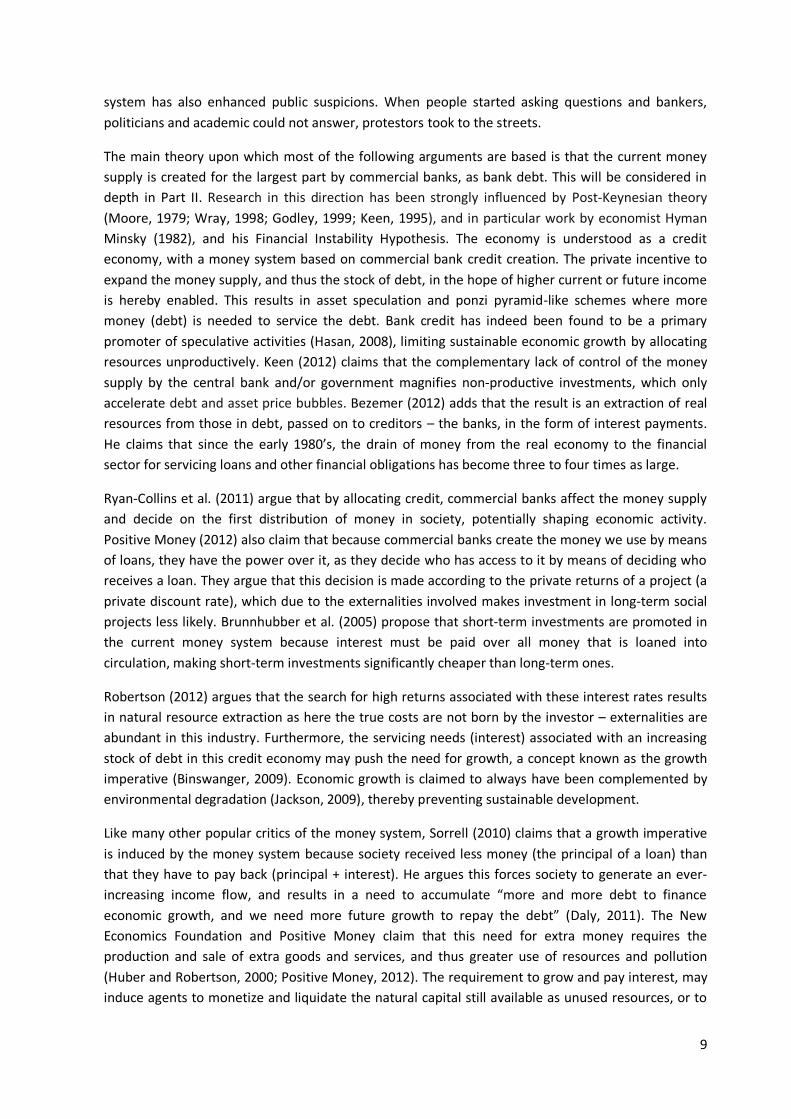
4.2. Empirical evidence.

The scope of degradation that humans impose on the environment is immense. It ranges from

biodiversity losses to resource depletion to landscape pollution. Figure 14 presents a general

overview of some basic environmental indicators.

Figure 14. Indicators of Human Activity and the State of the Environment (Steffen et al., 2004).

30

Considering the main trends in these indicators, they all point in the same direction, away from what

is sustainable since the 1900s. Indicators of the state of the atmosphere reveal increases in CO2, N2O

and CH4 concentrations as well as a degrading ozone layer. Coastal as well as terrestrial ecosystems

similarly show strain, as there are increasing losses in ecosystems, structure, and biodiversity.

A measure of fossil energy demand can be used as a representative, or at least illustrative indicator

of a variety of the environmental trends including “global warming, resource depletion, acidification,

eutrophication, tropospheric ozone formation, ozone depletion, and human toxicity” (Huijbregts et

al., 2006). Figure 15 gives worldwide fossil energy demand as well as global GDP for comparison, and

Figure 16 gives the same specifically for the UK, adjusted for imports and exports of fossil energy.

Note that a total energy demand is given, not corrected for GDP or population changes because the

absolute trends are important as these impact the environment. The difference between relative and

absolute trends will be further discussed below.

Figure 15. Global fossil energy consumption and GDP (World Bank, 2012).

Figure 16. Total Primary Fossil Energy Use and GDP in the UK (IEA, 2010; World Bank, 2012).

Worldwide fossil energy consumption, and the related activities, have been increasing steadily.

Compared to GDP, the trends are very similar. The link between environmental degradation will be

0

5E+12

1E+13

1.5E+13

2E+13

2.5E+13

3E+13

3.5E+13

4E+13

4.5E+13

0

2000000

4000000

6000000

8000000

10000000

12000000

1971

1973

1975

1977

1979

1981

1983

1985

1987

1989

1991

1993

1995

1997

1999

2001

2003

2005

2007

2009

GD

P (

con

stan

t 200

0 U

S$)

Glo

bal

Fo

ssil

Ener

gy C

on

sum

pti

on

(k

toe)

Year

Fossil Energy Consumption

0

2

4

6

8

10

12

14

16

18

20

0

5000

10000

15000

20000

25000

30000

1971

1973

1975

1977

1979

1981

1983

1985

1987

1989

1991

1993

1995

1997

1999

2001

2003

2005

2007

2009

GD

P (

*10^

11

, co

nst

ant 2

000

US$

)

Tota

l pri

mar

y en

erg

y su

pp

ly (k

toe

)

Fossil Energy Consumption

GDP (constant 2000 US$)

31

further discussed in a later section. Worldwide fossil energy consumption has almost doubled since

1971. According to most estimates, we are either nearing global ‘peak’ oil, or have already surpassed

it (Hirsch, 2006) and thus global production rates will commence to decline, lasting at current

expectations another 40 years (EIA, 2006). Gas and coal reserves are similarly rapidly being exploited,

enough for about 60 and 150 years respectively at current production rates (EIA, 2006), while on

average the world still depends for 80% on fossil fuels for its energy (World Bank, 2008). The UK is

even more dependent on these non-renewable resources, 88% of its energy is derived from fossil

fuels (World Bank, 2008). On the one hand this indicates there remain a number of decades to find a

solution, and technology may aid enhancing yields or the creation of new reserves. On the other

hand, production rates may be more likely to increase than decrease with a growing population and

various industrializing nations, reducing the above estimates. A true energy transition provides a

significant challenge as compared to other innovations that have been made in the past century.

In terms of the trends in fossil energy consumption of the UK, there is a decline in consumption from

1998 onwards, following a steep almost five-fold increase. This is likely to have been a result of

increasing dependence on imports for more fossil fuel intensive goods, as well as goods in general as

industrial production moves abroad. Considering statistics on the share of sectors in the UK, industry

is found to be losing ground to the service sector, from adding just over 40% to GDP in 1970, to a

mere 22% in 2010 (World Bank, 2012). There is, however, no clear indication as to why the decrease

in energy consumption occurred around 1998. Mainstream statistics do not consider the embodied

energy in imported goods and so even the above used statistics that incorporate imports of energy

(e.g. oil, gas, coal) do not reveal the true energy consumption of the country. The decrease in the UK

is likely to have been compensated for by increases in Asian exporting countries where industrial

production is increasing. To take this into consideration, there are some statistics that attempt to

consider the global footprints of nations, individuals or firms. These are discussed below.

Although a large variety of environmental indicators are covered by the proxy fossil energy demand,

Huijbregts et al. (2006) state that land use is not represented well enough. Therefore, another

general indicator of environmental performance is given in addition. This is the ratio of the world’s

ecological footprint (impact of production and consumption) to the Earth’s biocapacity as provided

by the Footprint Network (2011). Simply interpreted, this is the number of Earths humans require to

fulfill their current levels of consumption. The footprint includes (also energy) resources consumed

across the world, wastes generated and disposed of beyond borders, and it assumes current

technology levels and resource management. Figure 17 reveals an increasing world demand on the

Earth natural resources since 1960. The ratio given illustrates the deficit between the biocapacity

that the Earth provides, and the population’s demand. Country population sizes are controlled for: if

we compare between nations we compare the environmental pressures of the lifestyle of an average

citizen in each country. A value below one indicates we are not utilizing the Earth’s full capacity,

while any value above one indicates an overshoot of the Earth’s capacity.

32

Figure 17. Ratio of the World and the UK’s Ecological Footprint to the Earth’s Biocapacity (Footprint Network, 2011).

The world exceeded the Earth’s natural boundaries since around 1970. Its current demand of more

than 1.5 ‘Earths’ would be even more severe if the world’s population lived according to British living

standards. Interestingly, there was a decreasing trend in the demand on the Earth’s biocapacity by

the UK from 1975-1985, due to the economic crises that occurred in this time period resulting in

mainly lower demand and a decrease in energy intensity (Unander, 2007). However, ever since,

exploitation and pollution of the world's energy resources, seas, forests, and land continues to

increase back to the extremely high pre-1970 levels. Mankind is already living beyond the Earth’s

capacity, and there is an increasing global trend at which this occurs.

Considering a few resources more specifically, reveals that global consumption of cement, steel,

paper, aluminum and thermoplastics (Figure 18) as well as freshwater use (Figure 19) are even more

clearly increasing.

Figure 18. Rising Global Demand for Cement, Steel, Paper, Aluminum and Thermoplastics (Allwood et al., 2011).

0.5

1

1.5

2

2.5

3

3.5

4

4.5

5

1961 1965 1970 1975 1980 1985 1990 1995 2000 2005 2008

Glo

bal

Eco

logi

cal F

oo

tpri

nt t

o

Bio

cap

acit

y R

atio

World

United Kingdom

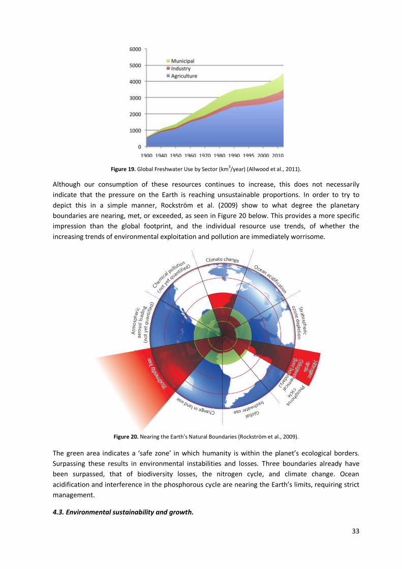
33

Figure 19. Global Freshwater Use by Sector (km3/year) (Allwood et al., 2011).

Although our consumption of these resources continues to increase, this does not necessarily

indicate that the pressure on the Earth is reaching unsustainable proportions. In order to try to

depict this in a simple manner, Rockström et al. (2009) show to what degree the planetary

boundaries are nearing, met, or exceeded, as seen in Figure 20 below. This provides a more specific

impression than the global footprint, and the individual resource use trends, of whether the

increasing trends of environmental exploitation and pollution are immediately worrisome.

Figure 20. Nearing the Earth’s Natural Boundaries (Rockström et al., 2009).

The green area indicates a ‘safe zone’ in which humanity is within the planet’s ecological borders.

Surpassing these results in environmental instabilities and losses. Three boundaries already have

been surpassed, that of biodiversity losses, the nitrogen cycle, and climate change. Ocean

acidification and interference in the phosphorous cycle are nearing the Earth’s limits, requiring strict

management.

4.3. Environmental sustainability and growth.

34

4.3.1. The decoupling myth.

Historically, environmental degradation has been a result of economic growth (Boulding et al., 1966;

Mishan, 1967). Resources are needed to grow, and more resources have been used during periods of

growth. However, there have been attempts to separate these two tendencies. Decoupling entails

that production and consumption (growth) occurs with fewer material resources and thus less

environmental degradation. The difference between absolute and relative decoupling is described in

a report on decoupling by UNEP (2011). Absolute decoupling implies a true decrease in

environmental degradation. Relative decoupling brings about a reduced energy and material

throughput per unit of economic output and population. Ecological impacts reduce compared to

GDP. This is rather an increase in efficiency and may not involve an absolute decrease in natural

resource use. The Environmental Kuznets Curve (Figure 21) illustrates how after a certain level of

income is reached, energy and material throughput can decrease for a number of reasons including

dematerialization, better regulation, saturated infrastructure demand and improved technologies

(Bernardini and Galli, 1993).

Figure 21. Environmental Kuznets Curve (Yandle et al., 2000).

There is evidence that illustrates such relative decoupling in the form of reduced energy and

resource intensities (EIA, 2008). Figure 22 shows the intensity of material use of economic growth in

five Western nations, revealing a steady downward trend.

Figure 22. Decrease in Material Intensity Reveals Relative Decoupling (Jackson, 2009).

Similarly, the world’s carbon intensity decreased by about 25% between 1980 and 2006, and its

energy intensity decreased even more, by about 33% since 1970 (Jackson, 2009). Although these are

positive trends, there is little evidence that absolute decoupling of the economy is possible, and total

35

natural resource (material and energy) use as well as emissions have continued to increase (Stern,

2004). The aforementioned improvements have been mainly visible in Western nations, and as the

rest of the world develops further their resource use is likely to simultaneously increase despite

increased efficiency. Indeed the use of metal continues to increase as developing nations build up

their economies (Figure 23).

Figure 23. World Primary Metal Extraction (Jackson, 2009).

Note that the increase in World GDP is lower than the increase in consumption of four out of five

metals, indicating there is not even relative decoupling. Figure 24 shows that even in the five

Western nations in Figure 22, material use has generally increased.

Figure 24. Increase in Material Consumption Reveals no Absolute Decoupling (Jackson, 2009).

Material consumption has increased since 1975, but is recently stabilizing. It is possible that this is

due to a transfer of material and energy intensive sectors to other countries, which would have only

relocated the problem. The above statistics do not consider the energy and materials that are

embodied in imported goods. Indeed, the UNFCCC (United Nations Framework Convention on

Climate Change) reports a decrease in emissions in the UK of 6% between 1990 and 2004, but if

emissions embodied in traded goods are considered, this becomes an 11% increase (Druckman and

Jackson, 2008)! The relationship that is proposed by the Environmental Kuznets Curve as outlined

above, may simply be a measure of “the ability of consumers in wealthy nations to distance

themselves from the environmental degradation associated with their consumption” (Rothman,

1998). It has also been found to only hold for local and visible environmental effects. For more global

issues and impacts that are easier to externalize or more expensive to deal with (i.e. resource

extraction, biodiversity losses, greenhouse gas emissions, waste generation) the relationship does

not hold (Booth, 2004). In these cases there is no decrease in environmental degradation and

resource use. Absolute decoupling would require a decrease in total demand for material and energy

resources, which we have seen is not the case.

36

In Prosperity Without Growth, Tim Jackson (2009) discusses the conventional claim that decoupling is

possible. He shows that economic growth, as we know it, will always require resources and energy,

with associated environmental damage and decoupling is a myth. Jackson’s argument is based on the

Ehrlich equation below which states that the environmental impact equals the population multiplied

by its income level times the technological intensity of economic output.

(1)

Relative decoupling occurs when decreases. This becomes absolute decoupling if the total impact

( ) decreases, which only occurs if the rate of relative decoupling (the decrease in ) is greater than

the growth rates of population ( ) and income ( ) together. Sustainable growth is growing in per

capita terms at a rate that equals the dematerialization rate minus the population growth rate

(possibly a negative number).

Given historical evidence and future possibilities, such a growth rate seems highly unlikely. Since

1990, population and income have seen a 2.7%/year increase together, and considering the case of

climate change and carbon intensities, there has only been a 0.7%/year decrease in the intensity of

emissions (Jackson, 2009). Furthermore, to be able to achieve the IPCC’s (International Panel on

Climate Change) current target of 450ppm, at the same population and income growth rates, Jackson

calculates emissions per dollar would need to fall by 4.9% annually up to 2050. Arguably, the global

population may grow less rapidly in future years, which would reduce the needed reduction in

intensity to some degree. On the other hand, if the developing world hopes to reach Western living

standards, the growth in the level of affluence will increase significantly more. These different

scenarios are presented in Figure 25.

Figure 25. Carbon Intensities Required to Meet 450ppm Carbon Emissions Target (Jackson, 2009).

In the most undemanding scenario, at current income growth, and just 9 billion people in 2050, the

world’s carbon intensity would need to decrease about 7.3%/year, from 768gCO2/$ to 36gCO2/$. At

the same 2050 population, but more equitable world income at the EU 2007 level, with not only the

developing world growing but also a 2% annual growth rate in the West, the carbon intensity would

have to decrease about 11.4%/year! Considering that the carbon intensity has only decreased by

37

0.7% annually since 1990, this will be very difficult. It would require either a declining population, a

decrease in economic growth, or an immense technological breakthrough.

Once it is not possible to decouple economic growth from environmental degradation, any

mechanism that creates a necessity for the economy to grow at the current or a higher population

level, will naturally hinder sustainable development. It is therefore in our interest to determine

whether our money system causes a growth imperative; this will be done in Part III, based on this

section’s clarification of the concept.

4.3.2. The growth imperative.

The analysis above revealed that in order to reduce the impact of human activity, we either need a

decrease in population (consider Malthus, 1798), an immense innovation, or a reduction in growth.

However, there are arguments that the latter is not possible in our current system because it has a

growth imperative. This entails that the current economic-financial system requires economic (GDP)

growth in order to ‘survive’. All despite the fact that subjective well-being does not increase after a

certain level of GDP (Blanchflower and Oswald, 2004), as also seen in the previous chapter on human

sustainability.

Competition within the market place is an important reason why businesses individually experience a

growth imperative. They need to innovate in terms of their products, technology, and marketing in

order to outcompete other market participants. However, this does not necessarily translate to a

growth imperative at the national level because some firms lose in the competition and go bankrupt

while others outlast their rivals. In the aggregate, this could balance to a negative, zero, or positive

growth rate. Gordon and Rosenthal (2003) do claim to derive a growth imperative in the capitalist

system as a whole. They base their analysis on the risk of bankruptcy for firms if there is zero or

negative growth in consumption, investment, and the capital stock. Agents in the economy,

specifically capitalists, are driven towards behavior that induces growth in their own firms, no matter

what their rate of profitability or other variables are, to reduce the risk of bankruptcy to an

acceptable level. To account for variability in circumstances and profits, the firm furthermore not

only needs a positive, but also a high mean growth rate. The authors find that in the long-run, a no-

growth policy makes bankruptcy almost certain. They claim that as opposed to a socialist system in

which profits are redistributed through government and firms are secured from bankruptcy,

capitalism subjects itself to a growth imperative. However, the link between the individual firm that

has a growth imperative, and the aggregate economy remains unclear. Bankruptcy in the capitalist

system, so specifically considered in Gordon and Rosenthal’s model, could still result in a net zero or

positive growth rate, especially if it applies to the least growth firms.

Other research on the subject is done by Binswanger (2009). He alters the argument slightly, and

derives that a high mean growth rate in the economy is needed because of the credit economy we

are in, which otherwise does not realize or allow for profits for firms in the aggregate. He utilizes a

circular flow model to model interaction between components of the (credit) economy: banks,

households and firms. Banks make loans to firms, pay wages, and retain some of their interest

income as owner’s capital (equity). Households receive wages as well as dividends, and spend their

income. Firms undertake production over time, make loans to invest, pay interest to the banks,

wages to households, and experience capital depreciation.

38

The firms are driven towards growth-enhancing behavior in order to obtain and subsequently pay

back the loans with which they commence their business or make investments. Binswanger argues a

firm namely requires significant profit expectations in order to obtain the loan, either from the bank,

or from other investors, as these parties demand future cash flows. Any firm on the stock exchange is

even more tightly subject to these expectations of future dividends, further requiring profits. If

investments are not made, profitability decreases, and once it is past a certain threshold level, a

vicious cycle commences as these profitless firms stop investing. Similarly, when the creation of

marketable output fails for some reason, a firm is more likely to go bankrupt as also explained by

Gordon and Rosenthal (2003). In addition, Binswanger claims that because banks extract a part of the

money circulating through interest payments as owner’s equity, the money supply has to expand to

compensate in order for firms to continue to make profits in the aggregate. He finds that this

monetary inflow can only be sustained by a growing economy, yielding a growth imperative.

However, Binswanger finds that this minimal growth rate is just 0.45% per year.

The minimum growth rate required to ensure firms make profits in the aggregate depends on three

conditions. Firstly, when interest rates are high, firms have higher servicing costs and thus the rate is

higher. Secondly, if the banking sector as a whole retains more of its interest income, more of firms’

interest payments are not retrieved forcing them to retrieve these elsewhere – through higher

growth. Thirdly, when capital depreciates faster such as in times of transition or reform, it has to be

replaced more often requiring more (costly) investment and growth to be able to obtain and pay

back the loans needed to make these investments. Both Binswanger (2009) and Gordon and

Rosenthal (2003) find that in such times of greater uncertainty, the current system requires a higher

rate of return and a stronger growth imperative for firms.

A long-run zero-growth rate is not possible, because of the positive feedback created by banks

controlling the credit (and money) supply and because production takes time. This results either in

upward or downward spirals for firm profits in the aggregate and the economy’s growth rate in

general. As the firm’s failure has a high private cost, while the costs of growth are frequently social,

(global) externalities, an individual (private) agent in the current economic system has an incentive to

grow.

4.3.3. A zero-growth economy.

The link between environmental degradation and economic growth has been widely researched.

Already in 1972, The Limits to Growth by D. Meadows warned that exponential economic growth is

unsustainable, and that we would surpass the Earth’s natural boundaries within a century, resulting

in overshoot and collapse. If this is so, the ‘growthmania’ in which we reside, requires a drastic

change towards a more steady-state economy (Daly, 1977). Note that this interpretation of a steady

state economy is different from the constant growth rate definition in Economics. It is defined by

Daly as “an economy with constant stocks of people and artifacts, maintained at some desired,

sufficient levels by low rates of maintenance "throughput", that is, by the lowest feasible flows of

matter and energy from the first stage of production to the last stage of consumption” (Daly, 1977).

There is thus a zero-growth rate, which is claimed to be needed by various researchers after

centuries of environmentally degrading growth. Simms and Alanson (2010) write “infinite growth

isn’t possible” in a world with a limited stock of physical resources, due to the material nature of

economic growth. The alternative is a steady-state economy. “The world is finite, the ecosystem is a

39

steady-state. The human economy is a subsystem of the steady-state ecosystem. Therefore at some

level and over some time period the subsystem must also become a steady-state, at least in its

physical dimensions of people and physical wealth. The steady-state economy is therefore a physical

necessity” (Daly, 1973). This is an economy where birth and death rates as well as physical

production and consumption rates are balanced at their highest ecologically feasible level. Although

the financial economy is potentially limitless because money can grow forever, in real terms this is

not so: real financial wealth is linked to and limited by the real economy also through the price

mechanism. These authors claim that only in this manner, can we achieve a sustainable society.

4.4. Conclusion.

Bringing these theoretical concepts together with the empirical analysis on the state of the

environment in the first part of this chapter, reveals that economic (GDP) growth is not sustainable

to date. The indicators reveal excessive extraction, as well as pollution both globally and nationally in

the UK. Ecological boundaries have, or are being exceeded. The Earth’s natural resources continue to

be exploited and degraded, ‘liquidated’. It is beyond the scope of this paper to analyze the effect of

the money system on each of these trends, but the relationship with economic growth that was

given above provides a useful bridge and a single indicator to consider in Part III. Economic growth,

as defined by a growth in GDP, cannot be complemented by an absolute reduction or stabilization of

physical production and consumption due to the limitations of decoupling. Furthermore, the

proposed alternative steady state economy would be impossible in an economy with a growth

imperative. Together, these mechanisms impede environmental sustainability. Part III will investigate

whether the present money system induces such a growth imperative, and in that way hinders

environmental sustainability.

40

CHAPTER V – PILLAR 3 : ECONOMIC SUSTAINABILITY

5.1. Introduction.

The third pillar of sustainability concerns the need for an efficient, competitive, and resilient

economy to enable ensure that the needs of the current and future generations are met. It is needed

for the optimal allocation of natural and human resources within the discussed ecological and social

constraints. Internally, this pillar embodies the need of humans to improve their situation relative to

the past and their peers, the need for added value, innovation, entrepreneurship, and progress

(Garrett, 2010). Externally, a society needs a strong economy to be resilient in a constantly evolving

(global) market. This is also needed to enable the large investments and innovations that are

required to make the transition to a sustainable society. This chapter first presents the increasing

financialization of our current economy, focusing on the UK. It then explores trends in the financial

sector that may give an indication of what this means for the efficiency, competitiveness, and

resilience of the economy. I find that although on the surface increasing income and efficiency

indicate a strong economy, a low degree of competition, risk-weighted productivity, and real

investments may limit the long-term resilience of the economy. The chapters ends with a final

indication of the financial challenge at hand to develop a sustainable society.

5.2. Financialization of the economy.

The economy today is characterized by an increasingly important financial sector. The state of the

financial sector has become of great influence on the economy and society at large. The introduction

already presented how the current crisis has shown that when the financial sector is in bad shape,

society follows. High levels of unemployment, increased poverty, a drop in bank lending, and

stagnating economic growth currently characterize the US and Europe (European Commission, 2009).

The crisis also increased investments in natural resource based commodities (Buiter, 2007; Buscher,

2011; Gorton and Rouwenhorst, 2006) increasing the strain on the environment. We are in the

middle of experiencing the impact of a failing financial system, and so far have not been able to

recover.

This process of ‘financialization’ is described by Krippner (2005) as a “pattern of accumulation in

which profit making occurs increasingly through financial channels rather than through trade and

commodity production”. It is a general process much like globalization, encompassing various trends

such as increased importance of maximizing shareholder value, increasing dominance by an elite

rentier class, an increase in complex financial products and innovation (Stockhammer, 2004; Epstein,

2005; Dore, 2008). Figure 26 reveals the growing importance that the sector has been gaining over

the past decades.

41

Figure 26. Size of the UK Banking System(left) and Real Gross Value Added in the UK (right) (Haldane et al., 2010).

After a period of stability between 1880 and 1970 where banking sector assets were about 50% of

GDP, a rising trend has increased this to its current value of more than 500% of GDP in the UK. Since

the 1980s, the financial sector’s value added has also grown much more rapidly than that of the

economy in its aggregate. On average, over the past 160 years, the growth in value added of financial

intermediation has been about 2% per year higher than of the aggregate economy, and its share of

total profits in the economy has increased from an average 1.5% between 1948 and 1978, to 15% in

2008 (Haldane et al., 2010).

Over time, the sector has accordingly drawn in labor and capital. Between 1977 and 1990, the share

of workers employed in the financial industry increased about 50% to 4.5% of whole economy

employment, and the share of real capital allocated to the sector increased three-fold from 4% to

12% (Haldane et al., 2010). Since the 1980s, the financial sector not only increased the share of

employment in quantitative terms, but it also captured a larger share of the talent in the economy as

it hired skilled workers at a higher rate than other sectors (Philippon and Reshef, 2007). The

difference in educated (employees with more than a high school education) shares of the financial

sector and the non-agricultural private sector was 0.1 in 1970, and grew to 0.2 by 2005 (Philippon

and Reshef, 2008). More specifically, Goldin and Katz (2008) find that an increasing share of Harvard

undergraduates work in the financial sector since 1970. At the Massachusetts Institute of

Technology, 18% of graduates started work in the financial sector in 2003, and three years later this

was already close to 25% (Kedrosky and Stangler, 2011). Baumol (1990) as well as Murphy, Shleifer,

and Vishny (1991) argue that this increasing flow to intermediary (rent-seeking) sectors such as law

and finance is not desirable because the social returns of these sectors are lower than the high

private returns to ability that attract the talent. However, finance also has a positive effect on growth

(Levine, 2005), which makes these trends beneficial for the economy. The increase in skill intensity of

the sector can help to explain why the share of labor and capital captured by the financial sector

stabilizes around 1988, and even starts to decrease to just under 4% and 10% respectively in 2008

(Haldane et al., 2010). This indicates an increase in productivity, since value added continued to

increase.

Indeed, the sector’s measured productivity has grown at a far more rapid speed than the economy’s

average. Total factor productivity (TFP) of the financial sector has grown by 2.2% per year from 1995

to 2007, compared to 0.5-1% for the general economy (Haldane et al., 2010). Figure 27 shows that

this was not a trend unique to the UK.

42

Figure 27. Difference in TFP Financial Intermediation and Aggregate Economy (Haldane et al., 2010).

Figure 27 also shows that a large portion of the increase in productivity occurred between 2003 and

2007. Note also that in France, Sweden, Germany, and Austria the financial sector did not

outperform the general economy, though in all these countries except Germany it did between 2003

and 2007. The sector has accordingly been characterized by high returns to equity (Figure 28).

Globally, as well as in the UK the returns were about twice as high as those of non-financial firms

(Haldane et al., 2010). Later, we will see that these returns have not been real returns, but merely a

‘mirage’.

Figure 28. Return on Equity of Global (left) and UK (right) Banks (Haldane, 2012).

In addition to the generally rising trend, there have been especially high peaks in returns on equity

leading up to the crisis. These drop significantly when the crisis started, and have now returned to

levels experienced decades earlier. Weekly earnings in the UK financial sector are also high compared

to other industries (Figure 29).

43

Figure 29. Average Weekly Earnings of UK Industries (Haldane et al., 2010).

Only mining and quarrying industries make similar average weekly earnings. The next industry,

utilities, lies almost 40% lower in its earnings. In the Introduction higher wages in the financial sector

were found to be an important contributor to income inequality in the UK. Excessive wages in this

sector is not only the case in the UK, Figure 31Figure 30 shows the excess wage paid in the US

financial industry as compared to a benchmark average of all other sectors.

Figure 30. Historical Excess Wage in the Financial Sector (Philippon and Reshef, 2008).

Again, the financial sector has experienced higher earnings and wages than other sectors; in

particular between 1920 and 1940, and between 1990 and 2010. One would be led to believe that

given the rising importance of the financial sector in the economy, these trends are positive.

5.3. Trends in finance.

However, what seems like a natural process of allocation to where real returns and value-added are

highest, may merely be a question of measurement. Haldane et al. (2010) speak of a ‘productivity

mirage’. They find that rising productivity levels have been largely due to an increase in risk-taking in

an attempt by commercial banks to increase their return on equity. This has resulted in reported

returns increasing, but risk-adjusted returns on equity did not (Haldane, 2009). The greatest portion

of the increase in returns as well as in value added were simply been due to increased risk-taking and

leverage, not due to productivity gains (Haldane et al., 2010).

44

Furthermore, distortions in the system have hidden (social) costs and resulted in the allocation of

resources in unproductive financial and speculative investments. Government and central bank

policy subsidize private returns in this sector (Leijonhufvud, 2012). High and therefore risky leverage

ratios, backed by tax-payers’ money in multiple ways, enabled banks to speculate and manipulate

markets to gain the high returns on equity given in Figure 28. The exploitation of the various

opportunities that existed was rational from a private perspective. However, the costs of default and

risks of bankruptcy were socialized – insured by society (Admati, 2012), while the profits are private.

An increasingly concentrated financial sector enabled the development of ‘too big to fail’ institutions,

which could take such excessive risk at the expense of the taxpayer (Admati et al., 2011). The

concentration of the banking sector has increased immensely since the 1980s across the world; in

the UK, the top 3 banks currently own more than 50% of the total assets of the banking sector

(Haldane et al., 2010). Figure 31 gives the concentration of market power of US banks between 1935

and 2008.

Figure 31. Concentration of US Banks From 1935-2008 (Haldane et al., 2010).

The top 3 banks in the US own just over 40% of the banking sector’s total assets, a four-fold increase

since 1990. Globally, the share of the top three banks in the banking sector’s total assets has doubled

since 2000 (Haldane et al., 2010). Decreasing competition increases monopoly power and has the

potential to allocate resources in a suboptimal manner to the benefit of the monopolistic

competitors. It reduces the contestability of the market as entry and exit is no longer free. Pistor

(2012) claims that the financial system respects, and even entrenches existing skewed national as

well as global hierarchies. The most liquid institutions, not only in terms of their own accounts, but

also in terms of the chance they are bailed out if things go wrong, are at the top of the hierarchy and

allocate capital to those that are willing to pay most, not according to merits. The lack of a level

playing field reduces the efficiency of the market, which can misallocate capital, distort investment,

and cause instability (Minsky, 1986).

At the same time, competition between those at the top of the hierarchy, drives the sector towards

investments of which they are able to acquire part of the gains (loans private benefits), fastest (short-

term loans), with less risk (collateral based loans), and away from the social, long-term investments

45

required to make the transition towards a sustainable society. This creates a dilemma between

private and public actions, because what is efficient from an individual perspective, is inefficient or

even undesirable from a social perspective. Particular institutions are required to turn this around; to

strike a balance between the public and private realm to hope to find the best way forward for all.

Deregulation of the financial sector has been a key driver of these changes. (De)regulation has been

based on perfectly competitive markets, efficient, with perfect information, and free liquidity; i.e.

“imagined, not real markets” (Pistor, 2012). It has enabled the finance, insurance and real estate

(FIRE) sectors to grow almost three-fold since the 1980s (Bezemer, 2012), in a continuous search for

private profits in any way possible. It has led to an increasing discrepancy between debt and GDP

levels, as credit to the financial (FIRE) sector increased which drove up asset prices, induced

speculation, and inflated debt-to-GDP ratios in many Western nations (Bezemer, 2012). Bezemer

argues that credit to the financial sector is not invested in the real economy and therefore does not

directly create real economic investment and growth. Figure 32 depicts the trends in debt-to-GDP

ratios of a number of nations since 1990, with an indication of the start of the deleveraging process.

Figure 32. Total Debt-to-GDP Ratio in Ten Developed Economies (Roxburgh et al., 2012).

All nations have experienced rising debt-to-GDP ratios since the 1990s, and in particular the UK.

Bezemer claims this has increased the systemic leverage of economies to unsustainable levels, since

a sustainable real-economy enhancing level of debt-to-GDP is 100%, which all these nations are far

above. Given the lack of efficiency and competitiveness in the economy because of the role of the

financial sector, the current system has likely failed in allocating resources in an optimal manner.

46

5.4. Trends in financial sector lending and investment.

Evidence on financial sector lending shows that indeed the real economy plays a relatively small role.

Figure 33 gives a breakdown of total lending by financial institutions in the UK to UK residents.

Figure 33. Loans made by Financial Institutions in the UK by Destination (Bank of England, 2012).

Until the end of 2008 the total amount of loans increased, followed by about a year in which the

total number remained reasonably constant. In the end of 2008 a sudden jump increases the

amounts outstanding to over 2,500,000 million pounds sterling at the beginning of 2010. However,

ever since the total has been decreasing, currently standing at the start of 2008 levels. The increase

was a result of significant increases in loans to other financial institutions, as well as an increase in

secured loans to individuals. These two elements are components of lending to the FIRE sector.

To consider in particular the credit allocated per sector, Figure 34 graphs the share of total loans

outstanding for the individual sectors and to the FIRE sector as a whole.

0

500000

1000000

1500000

2000000

2500000

3000000 se

p-9

7

mar

-98

se

p-9

8

mar

-99

se

p-9

9

mar

-00

se

p-0

0

mar

-01

se

p-0

1

mar

-02

se

p-0

2

mar

-03

se

p-0

3

mar

-04

se

p-0

4

mar

-05

se

p-0

5

mar

-06

se

p-0

6

mar

-07

se

p-0

7

mar

-08

se

p-0

8

mar

-09

se

p-0

9 m

ar-1

0

sep

-10

m

ar-1

1

sep

-11

m

ar-1

2

Mo

nth

ly a

mo

un

ts o

uts

tan

din

g

(ste

rlin

g m

illio

ns

seas

on

ally

ad

just

ed

)

Unincorporated businesses and non-profit making institutions

Individuals for consumer credit

Individuals secured on dwellings

Other financial corporations

Private non-financial corporations

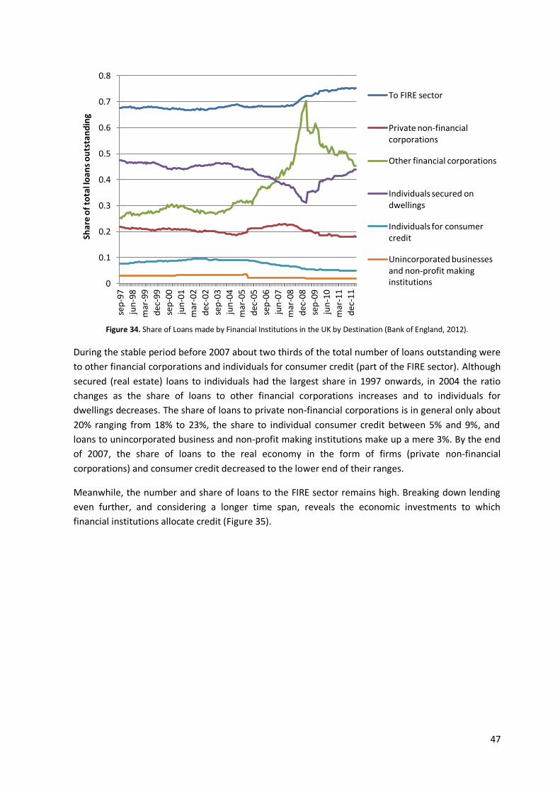
47

Figure 34. Share of Loans made by Financial Institutions in the UK by Destination (Bank of England, 2012).

During the stable period before 2007 about two thirds of the total number of loans outstanding were

to other financial corporations and individuals for consumer credit (part of the FIRE sector). Although

secured (real estate) loans to individuals had the largest share in 1997 onwards, in 2004 the ratio

changes as the share of loans to other financial corporations increases and to individuals for

dwellings decreases. The share of loans to private non-financial corporations is in general only about

20% ranging from 18% to 23%, the share to individual consumer credit between 5% and 9%, and

loans to unincorporated business and non-profit making institutions make up a mere 3%. By the end

of 2007, the share of loans to the real economy in the form of firms (private non-financial

corporations) and consumer credit decreased to the lower end of their ranges.

Meanwhile, the number and share of loans to the FIRE sector remains high. Breaking down lending

even further, and considering a longer time span, reveals the economic investments to which

financial institutions allocate credit (Figure 35).

0

0.1

0.2

0.3

0.4

0.5

0.6

0.7

0.8

sep

-97

jun

-98

mar

-99

dec

-99

sep

-00

jun

-01

mar

-02

dec

-02

sep

-03

jun

-04

mar

-05

dec

-05

sep

-06

jun

-07

mar

-08

dec

-08

sep

-09

jun

-10

mar

-11

dec

-11

Shar

e o

f to

tal l

oan

s o

uts

tan

din

g To FIRE sector

Private non-financial corporations

Other financial corporations

Individuals secured on dwellings

Individuals for consumer credit

Unincorporated businesses and non-profit making institutions

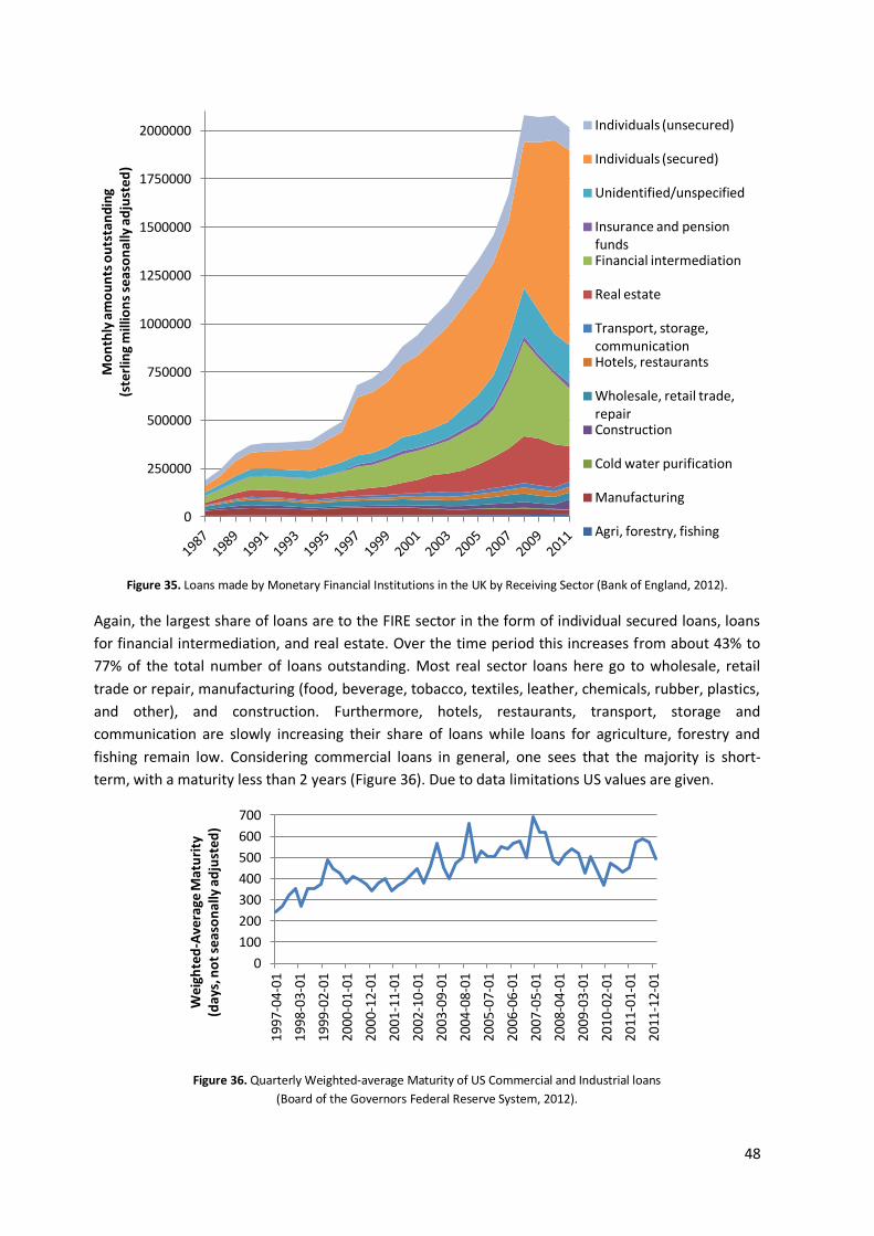
48

Figure 35. Loans made by Monetary Financial Institutions in the UK by Receiving Sector (Bank of England, 2012).

Again, the largest share of loans are to the FIRE sector in the form of individual secured loans, loans

for financial intermediation, and real estate. Over the time period this increases from about 43% to

77% of the total number of loans outstanding. Most real sector loans here go to wholesale, retail

trade or repair, manufacturing (food, beverage, tobacco, textiles, leather, chemicals, rubber, plastics,

and other), and construction. Furthermore, hotels, restaurants, transport, storage and

communication are slowly increasing their share of loans while loans for agriculture, forestry and

fishing remain low. Considering commercial loans in general, one sees that the majority is short-

term, with a maturity less than 2 years (Figure 36). Due to data limitations US values are given.

Figure 36. Quarterly Weighted-average Maturity of US Commercial and Industrial loans

(Board of the Governors Federal Reserve System, 2012).

0

250000

500000

750000

1000000

1250000

1500000

1750000

2000000

Mo

nth

ly a

mo

un

ts o

uts

tan

din

g

(ste

rlin

g m

illio

ns

seas

on

ally

ad

just

ed

) Individuals (unsecured)

Individuals (secured)

Unidentified/unspecified

Insurance and pension funds Financial intermediation

Real estate

Transport, storage, communication Hotels, restaurants

Wholesale, retail trade, repair Construction

Cold water purification

Manufacturing

Agri, forestry, fishing

0

100

200

300

400

500

600

700

1997

-04

-01

1998

-03

-01

1999

-02

-01

2000

-01

-01

2000

-12

-01

2001

-11

-01

2002

-10

-01

2003

-09-

01

2004

-08

-01

2005

-07

-01

2006

-06

-01

2007

-05

-01

2008

-04

-01

2009

-03

-01

2010

-02

-01

2011

-01

-01

2011

-12

-01

Wei

ghte

d-A

vera

ge M

atu

rity

(d

ays,

no

t se

aso

nal

ly a

dju

sted

)

49

Although the maturity of loans generally increased from 1997 until 2007, the crisis has caused the

average maturity of loans to decrease back to 2003 levels. Only after 2010 this slowly picks up again.

With banks extending loans at such short average maturities, it is difficult to make the long-term

investments necessary to achieve sustainable development. Even if the loans are rolled over, the

uncertainty that is complementary to such short-term commitments are expected to prevent robust

long-term investments. Similar trends are likely to exist in the UK, and is reflected in bank lending.

Meanwhile, a variety of ‘green’ investments are needed from a social and environmental perspective

(Lietaer, 2001). The latest World Energy Outlook (IEA, 2011) emphasizes the investments needed to

make the energy transition and secure future supply amounting to about US$ 1 trillion per year

worldwide until 20351. Of this, US$500 billion per year from 2010 to 2050 is for the power sector

only, US$150 billion to reach the 2°C target, US$300 billion for improving the efficiency of buildings,

and US$60 billion for industry. The remainder is spread out amongst various sectors. The Stern

Review (2007) suggested a cost of 1-2% of GDP to limit emissions to the 550ppm CO2e target by

2050. PriceWaterhouse Coopers conclude 3% of GDP is needed (PwC, 2008). Today, this would

require between US$800 billion and US$2.4 trillion per year until 2050 (CIA World Factbook: 2012).

For the UK, this would be about US$22.5 and US$67.5 billion per year until 2050 (CIA World

Factbook: 2012). Other recent estimates for the UK government’s Green Investment Bank by Vivid

Economics (2011) estimate annual investments will increase from US$45 to 80 billion up to and

beyond 2020 to stimulate the transition to a green economy. Energy investments alone will require

about US$320 billion (Ofgem, 2009), of which those for electricity generation and transmission make

up about US$170 billion (DECC, 2011). Ernst & Young (2010) have also made estimates for the capital

requirements of the green transition, arguing a total of about US$700 billion will be needed until

2025, about US$50 billion per year.

The investments needed are frequently of a public nature, for which the private incentives are

lacking (Hardin, 1968), reducing the probability that commercial banks will fund them. They are likely

to entail high levels of uncertainty of which the benefits only materialize in the long-term. Banks

prefer to extend loans to collateralized, large-scale projects, which are generally not the

characteristic of sustainable investments due to their innovative, risky, or decentralized nature.

Furthermore, recent trends show European and US financial institutions are steering away from their

traditional core business, which intermediates between those who have and need money across

space and time (Hoffman, 2007). This may further hamper investment in the green transition.

However, we have defined the functions of the financial system in our current economy as to

allocate resources in an efficient manner across space and time, share risk, and enable payments

(Crane, 1995). Note that the sector has never formally received this mandate of allocating money

and resources optimally, it is a private profit-seeking sector that has made this its business model,

and society has subsequently accepted. The financial sector has become very relevant for various

tools of inter-temporal and spatial equity such as interest, debt, and investment of resources which

makes it vital to achieve sustainability. Wray (2011a) indeed states that the financial system could be

a “tool for sustainable development”. It is needed as an efficient and competitive intermediary to

help make the transition investments. Unfortunately, this exploration has found this not be the case.

1 All values are in 2011 US dollars and global values are adjusted for purchasing power of parity.

50

5.5. Finance and growth.

In addition to its role in allocating existing funds, the financial sector is also argued to play an

important role in funding new real economic growth (Keen, 2012). There is an extensive amount of

empirical research on the finance-growth nexus, which finds that financial development is generally

positive for economic growth and that there is a strong empirical relationship between economic

(GDP) growth and credit to the real sector (see for example Levine, 2005). However, more

specifically, there is a strand of arguments that explain this importance of the financial sector with

the role of commercial banks in investments.

Both Keynes and Schumpeter stated that economic growth required a simultaneous increase in

purchasing power (the money supply), in the form of credit, which, provided by commercial banks,

places these institutions in a uniquely important position in the economy. Schumpeter (1927) wrote:

“Without the creation of new purchasing power by bank credits… financing of industrial

development in modern economies would have been impossible” and Keynes (1937) argued that

therefore “the banks hold the key position in the transition from a lower to a higher scale of activity”.

One needs an additional monetary injection in the form of credit for investments, because savings

reduce the stock of money. For an economy to grow and develop, “It is not sufficient… that savings of

yesterday be invested today, or, as it is often expressed, that investment offset savings. Investment

today must always exceed the savings of yesterday…. An injection of new money… must take place

every day” (Domar, 1957). As stated, this injection of money in the form of credit comes from

commercial banks. This is also needed because production takes time, the profits of an investment

come after the money required to fund them. This time lag is overcome by banks. For these reasons,

they play an important role in the economy in directing investments, including those required to

develop a more sustainable economy.

5.6. Conclusion.

This third pillar of sustainability requires an efficient, competitive, and resilient economy. Part III will

determine the effect of the money system on this pillar. I have focused on the financialization of the

economy, which gives the financial sector an increasingly important role in the stability of the

economy and society as a whole. Unfortunately, higher productivity levels of this sector may have

been largely due to higher levels of risk and leverage, questioning its true added value, and the

increased allocation of labor and capital to the sector. Public subsidies to the sector in the form of

guarantees and an increasing concentration of market power further distorted the efficiency of the

sector. Meanwhile, the sector plays an important role in allocating resources and enabling economic

growth through its role in credit creation. In the past decades, this has guided the economy towards

the FIRE sector, and the real economy makes up a relatively small share of total lending. Finally, an

estimate of the investments needed to make the transition to a sustainable society were given, as an

indication of the task at hand, which the financial sector will need to play a role in achieving.

51

REFERENCES

Admati, A. R., De Marzo, P. M., Hellwig, M. F. and P. C. Pfleiderer (2011). “Fallacies, Irrelevant Facts, and Myths in the Discussion of Capital Regulation: Why Bank Equity is Not Expensive”. Rock Center for Corporate Governance at Stanford University Working Paper No. 86.

Alesina, A. and R. Perotti (1996). “Income distribution, political instability, and investment”. European Economic Review 40.6: 1203-1228.

Alesina, A., Di Tella, R. and R. MacCulloch (2004). “Inequality and happiness: are Europeans and Americans different?”. Journal of Public Economics 88.9-10: 2009-2042.

Allwood, J. M., Ashby, M. F., Gutowski, T. G. and E. Worrell (2011). “Material efficiency: a white paper”. Resources, Conservation and Recycling 55.3: 362-381.

Baumol, W. J. (1990). “Entrepreneurship: Productive, Unproductive, and Destructive”. Journal of Political Economy 98: 893—921.

Bezemer, D. (2012). “Finance and Growth: When Credit Helps, and When it Hinders”. Prepared for the 3rd Annual INET Conference, Berlin.

Blanchflower, D. G. and A. J. Oswald (2004). “Well-being overtime in Britain and the USA”. Journal of Public Economics 88.7-8: 1359-1386.

BoE: Bank of England (2012). “Monetary financial institutions' balance sheets, income and expenditure”. Interactive Database.

Bernardini, O. and R. Galli (1993). “Dematerialization: Long-term trends in the intensity of use of materials and energy”. Futures 25.4: 431-448.

Binswanger, M. (2009). “Is There a Growth Imperative in Capitalist Economies? A Circular Flow Perspective”. Journal of Post Keynesian Economics 31.4: 707-727.

Blanchflower, D.G. and A.J. Oswald (2004). “Well-being over time in Britain and the USA”. Journal of Public Economics 88: 1359–1386.

Blanden, J. (2009). “How much can we learn from international comparisons of social mobility?”. Paper presented at Carnegie Corporation of New York and Sutton Trust conference on social mobility and education. New York, June.

Board of Governors of the Federal Reserve System (2012). “Weighted-Average Maturity for All C&I Loans, All Commercial Banks (EDANQ)”. Federal Reserve Economic Data.

Boulding, K. E. et al. (1966). Environmental quality in a growing economy. Baltimore: Alans Hopkins University Press.

Booth, D. (2004). Hooked on Growth – economic addictions and the environment. New York: Rowman and Littlefield.

Brunnhuber, S., Fink, A., and J. Kuhle (2005). “The financial system matters: future perspectives and scenarios for a sustainable future”. Future 37: 317-332.

CIA World Factbook (2012). “World”. The World Factbook. Retrieved 27 June 2012 from <https://www.cia.gov/library/publications/the-world-factbook/geos/xx.html>.

Creutz, H. (2010). The Money Syndrome. Northhampton: Adeolu Alao. Daly, H. E. (1973). Toward a Steady-state Economy. San Francisco: W. H. Freeman ------------ (1977). Steady-State Economics. San Francisco: W.H. Freeman. ------------ (2010). “From a Failed-Growth Economy to a Steady-State Economy”. The Solutions Journal

1.2: 37-43. DECC: Department of Energy and Climate Change (2011). “Planning our electric future: A White

Paper for secure, affordable and low-carbon electricity”. Retrieved 1 July 2012 from <http://www.decc.gov.uk/en/content/cms/legislation/white_papers/emr_wp_2011/emr_wp_2011.aspx>.

Domar, E. (1957). Essays in the Theory of Economic Growth. New York: Oxford. Dore, R. (2008). “Financialization of the global economy”. Industrial and Corporate Change 17.6:

1097-1112.

52

Druckman, A. and T. Jackson (2008). “The Surrey Environmental Lifestyle Mapping (SELMA) Framework – development and key results to date”. RESOLVE Working Paper 08/08. Guildford: University of Surrey.

Easterlin, R. A. (1974). “Does economic growth improve the human lot? Some empirical evidence”. In: David PA. and W. R. Melvin (eds.), Nations and households in economic growth. Palo Alto, Ca.: Stanford University Press.

------------------- (2001). “Income and happiness: towards a unified theory”. The Economic Journal 111: 465–484.

Egmond, N. D. van and H. J. M. de Vries (2011). “Sustainability: The search for the integral worldview”. Futures 43: 853-867.

EIA: Energy Information Administration (2008). International Energy Annual 2006. Washington DC: Energy Information Administration.

Epstein, G. A. (2005). Financialization and the World Economy. Cheltenham, UK: Edward Elgar. Ernst & Young (2010). Capitalizing the Green Investment Bank: Key issues and next steps. Retrieved 1

July 2012 from <http://www.green-alliance.org.uk >. Fong, C., Bowles, S., and H. Gintis (2004). “Reciprocity, Self-interest and the Welfare State”. In: C. A.

Gerard-Varrett (ed.), Handbook on Economics of Giving, Reciprocity and Altruism. Dordrecht: Elsevier.

Footprint Network (2011). Data retrieved 29 June 2012 from <http://www.footprintnetwork.org>. Garrett, T. A. (2010). “U.S. Income Inequality: It’s Not So Bad”. Federal Reserve Bank of St. Louis –

Inside the Vault Spring 2010. Retrieved 28 July 2012 from <http://stlouisfed.org/publications/itv/articles/?id=1920>.

Global Language Monitor (2012). “Top Words of the Decade 2000-2009”. Top Words. Retrieved 28 July 2012 from <http://www.languagemonitor.com/top_word_lists/>.

Goldin, C. and L. F. Katz (2008). “Transitions: Career and Family Lifecycles of the Educational Elite”. American Economic Review 98.2: 363-369.

Graedel, T. E. and R. J. Klee (2002). “Getting Serious About Sustainability”. Environmental Science & Technology 36.4: 523-529.

Haldane, A. G. (2009). “Small Lessons from a Big Crisis”. Bank of England Speech 397. Retrieved 28 July 2012 from <http://www.bankofengland.co.uk/publications/speeches/2009/speech397.pdf>.

Haldane, A., Brennan, S. and V. Madouros (2010). “What is the contribution of the financial sector: Miracle or mirage?”. In: The Future of Finance: The LSE Report: 87-120.

Hardin, G. (1968). “The Tragedy of the Commons”. Science 162.3859: 1243-1248. Henry, J. F. (2004). The Social Origins of Money: The Case of Egypt. In: Wray, L.R. (ed.), Credit and

State Theories of Money. Cheltenham: Edward Elgar. Hills, J. et al. (2010). An anatomy of economic inequality in the UK: report of the National Equality

Panel. London School of Economics and Political Science: Centre for Analysis of Social Exclusion. Hirsch, R. (2006). “Peaking of world oil production”. U.S. DOE National Energy Technology

Laboratory. HM Government (2009). The UK Low Carbon Transition Plan. Norwich: The Stationery Office. Huijbregts, M. A. J. (2006). “Is Cumulative Fossil Energy Demand a Useful Indicator for the

Environmental Performance of Products?”. Environmental Science & Technology 40.3: 641-648. IFS: Institute for Fiscal Studies (2004). Poverty and inequality in Britain: 2004. London: The Institute

for Fiscal Studies. IEA: International Energy Agency (2011). World Energy Outlook. Paris: International Energy Agency. IMF: International Monetary Fund (2000). World Economic Outlook May. Jackson, T. (2009). Prosperity Without Growth: Economics for a Finite Planet. London: Earthscan. Kaase, M. (1999). "Interpersonal trust, political trust and non‐institutionalized political participation

in Western Europe". West European Politics 22.3: 1-21. Kedrosky, P. and D. Stangler (2011). “Financialization and its Entrepreneurial Consequences”.

Kauffman Foundation Research Series: Firm Formation and Economic Growth.

53

Keen, S. (2012). “European Disunion and Endogenous Money”. Debt Deflation. Retrieved 18 Aug. 2012 from <http://www.debtdeflation.com/blogs/2012/07/03/european-disunion-and-endogenous-money/>.

Keynes J. M. (1937). “The ‘ex ante’ theory of the rate of interest”. In: D. Moggridge (ed.), The Collected Writings of John Maynard Keynes Vol. XIV. London: Macmillan, 1973.

Krippner, G. R. (2005). “The financialization of the American Economy”. Socio-Economic Review 3: 173-208.

Langenbacher, N. and B. Schellenberg (2011). Is Europe on the “Right” Path? Berlin: Friedrich-Ebert-Stiftung Forum.

Leipert, C. (1986). “Social Costs of Economic Growth”. Journal of Economic Issues 20.1: 109–131. Lélé, S. M. (1991). "Sustainable development: A critical review". World Development 19.6: 607-621. Levine, R. (2005). "Chapter 12 Finance and Growth: Theory and Evidence". Handbook of Economic

Growth 1.A: 865-934. Lietaer, B. (2001). The Future of Money, creating new wealth, work and a wiser world. London:

Century. Malthus, T. R., and G. Gilbert ([1798] 1993). An essay on the principle of population. Oxford: Oxford

University Press. Meadows, D. H. (1972). The Limits to Growth; a report for the Club of Rome’s project on the

predicament of mankind. NY: Universe Books. Milanovic, B. (2007). Worlds Apart: Measuring international and global inequality. Princeton:

Princeton University Press. Mishan, E. (1967). The costs of economic growth. London: Staples Press. Murillo-Zamorano, L. R. (2003). “Total Factor Productivity Growth, Technical Efficiency Change and

Energy Input. An International Frontier Analysis”. The University of York Discussion Papers in Economics No. 2003/09.

Murphy, K. M., Shleifer, A. and R. W. Vishny (1991). “The Allocation of Talent: Implications for Growth”. The Quarterly Journal of Economics 106.2: 503-530.

OECD (2008). Growing Unequal? Income distribution and poverty in OECD countries. Paris: OECD. Ofgem: Office of the Gas and Electricity Markets (2009). Project Discovery Energy Market Scenarios.

Retrieved 1 July 2012 from <http://www.ofgem.gov.uk/>. Perotti, R. (1996). “Growth, Income Distribution, and Democracy: what the data say”. Journal of

Economic Growth 1: 149-187. Philippon, T. and A. Reshef (2007). “Skill biased financial development: Education, wages and

occupations in the U.S. financial sector”. NBER Working Paper 13437. ----------------------------------- (2008). “Wages and Human Capital in the U.S. Financial Industry: 1909-

2006”. NBER Working Paper No. 14644. Pistor, K. (2012). Michael I. Sovern Professor of Law, Columbia Law School. Presentation at the 3rd

Annual INET Conference, Berlin. PwC: PriceWaterhouse Coopers (2008). The World in 2050. Retrieved 29 July 2012 from

<www.pwc.com/gx/en/world-2050/pdf/world_in_2050_carbon_emissions_08_2.pdf>. Robertson, J. (2012). Future Money: Breakdown or Breakthrough? London: Green Books. Rockström, J. et al. (2009). “A safe operating space for humanity”. Nature 461.7263: 472-475. Rothman, D. S. (1998). “Environmental Kuznets curves—real progress or passing the buck? A case for

consumption-based approaches”. Ecological Economics 25: 177-194. Roxburgh, C. et al. (2012). “Debt and deleveraging: Uneven progress on the path to growth”.

McKinsey Global Institute Report. Scheer, H. (2007). Energy Autonomy. London: Earthscan. Schumpeter, J. (1927). “Die goldene Bremse an der Kreditmaschine”. In: Kölner Vorträge Band I, die

Kreditwirtschaft 1. Leipzig: Gloeckner. Sen, A. K. (1993). “Capability and Well-being”. In: Martha C. Nussbaum and A. K. Sen (eds.), The

Quality of Life. Oxford: Clarendon Press. Simms, A. and V. Alanson (2010). Growth Isn't Possible. London: New Economics Foundation.

54

SIPRI (2012). SIPRI Military Expenditure Database. Retrieved 28 July 2012 from <www.sipri.org/databases/milex/>.

Steffen, W. et al. (2004). Global change and the earth system: a planet under pressure. Berlin: Springer.

Stern, D. I. (2004). “The Rise and Fall of the Environmental Kuznets Curve”. World Development 32.8: 1419–1439.

Stern, N. (2007). The Economics of Climate Change. Cambridge: Cambridge University Press. Stockhammer, E. (2004). “Financialisation and the slowdown of accumulation”. Cambridge Journal of

Economics 28.5: 719-741. Unander, F. “Decomposition of manufacturing energy-use in IEA countries: How do recent

developments compare with historical long-term trends?”. Applied Energy 84: 771-780. UN: United Nations (2010). The Millennium Development Goals Report 2010. New York: UN

Department of Economic and Social Affairs. UNEP: United National Environmental Program (2011). Decoupling natural resource use and

environmental impacts from economic growth. Paris: UNEP DTIE. Vivid Economics (2011). The Green Investment Bank: Policy and Finance Context. Department for

Business and Innovation Skills. Retrieved 1 July 2012 from <http://www.bis.gov.uk/greeninvestmentbank>.

WCED: World Commission on Environment and Development (1987). Our Common Future. Oxford: Oxford University Press.

Wilkinson, R. G., and K. Pickett (2009). The Spirit Level: why greater equality makes societies stronger. New York: Bloomsbury Press.

World Bank (2008). “World Development Indicators”. In: Kornblum, W., Sociology in a Changing World. Stamford, CT: Cengage Learning.

-------------- (2012). “World dataBank”. Retrieved 30 June 2012 from <http://data.worldbank.org>. World Values Survey (2008). “Values Studies”. Retrieved 29 July 2012 from

<www.wvsevsdb.com/wvs/WVSData.jsp>. Yandle, B., Vijayaraghavan, M., and M. Bhattarai (2000). Environmental Kuznets Curves: A Primer.

Bozeman: The Property and Environment Research Centre.

55

Part II – Money and its creation

In order to investigate whether there are implications of our current money system for sustainable

development it is vital to obtain an adequate understanding of this former variable – the nature of

money and our current money system. We need to answer questions such as: what is money, how

did money develop, what role does money play in economic models, and where does money come

from or who creates it? Authors from a variety of disciplines have described the history of money,

often commencing with a general understanding of the origins of money and subsequently

presenting the various interpretations of money across the globe and over time (see for example

Davies, 2002; Einzig, 1966; Galbraith, 1975; del Mar, 1880, 1895; and Weatherford, 1997). These

historical recollections have been widely researched and the reader is advised to refer to the

aforementioned sources for such details. For this thesis, different theories on the origins of money

will be considered as these influence the way in which we see money today.

This part is organized as follows:

Chapter 6: Defining money;

Chapter 7: The historical origins of money;

Chapter 8: Development of economic theory, thought, and models of the nature of

money and the money system;

Chapter 9: Our current money system.

First, a standard definition of money is presented as a starting point of this analysis. Money is

officially defined by means of a number of monetary aggregates, but also has a number of important

functions that will be considered. From this basic understanding, we delve into the history of money.

Second, the origins of money are discussed in Chapter 7 organized according to three main theories:

trade and commercial origins of money, sacred and religious origins, and social and State origins. This

chapter is based largely on historical and anthropological literature. The emphasis in these chapters

is on the first developments of money and despite strong archeological evidence it must be noted

that there remains uncertainty surrounding such finds due to the time period considered. Therefore,

56

I will also present how these different approaches to money have evolved over time and influenced

society in the more recent past.

Third, Chapter 8 will present the main developments in economic theory in particular on the role of

money in the economy. It commences with those Classical schools of thought that assume money is a

neutral factor in the economy, in the words of David Hume (1752): “the oil which renders the motion

of the wheels smooth and easy”. Over time, shortcomings of this basic model emerged due to its

simplification of reality. This led to new additions, and the general Keynesian understanding that

money does have an influence in the short-run. In the long-run, the equilibrating forces that are also

in the basic Classical model maintain money neutrality. However, according to various more

heterodox schools this approach still does not come close to modeling the economy realistically.

They assign an explicit and influential role to money in the economy in both the short- and long-run.

Understanding these different roles of money in economic thought is important because the

development of economic theory and thought on the nature of money have shaped the perceptions

of money of policy-makers as well as the general public. This chapter wraps up with a reflection on

these three economic approaches to money, which influences the interpretations of money later

applied.

Fourth, after these two historical overviews, Part II ends with Chapter 9 on the money system today.

It presents two different views on the way in which money enters our economy, and the subsequent

effects it has. The first view is denoted as the ‘old’ view, based on the money multiplier. The second

view is a ‘new’ view presented by a number of heterodox schools of economic thought as already

previewed in the prior chapter. These base their analysis of the money supply on the theory of

endogenous money.

The chapters of Part II and their individual sections build upon each other, not necessarily

chronologically, but in terms of a general understanding of the workings of the money system today

and its effects. This is the second building block, in addition to the first on sustainability, for the

analysis in Part III.

57

CHAPTER VI – DEFINING MONEY

6.1. Introduction.

Economics textbooks will define money somewhat along the lines of: “Money is the stock of assets

that can be readily used to make transactions” (Mankiw, 2008), or, “Financial assets that can be used

directly to buy goods” (Blanchard, 2011). This emphasizes the functional aspect of money as a

method of payment or means of exchange. Money is a stock variable, like financial wealth, while

income and saving are flows related to a certain time period. Another working definition of money

could be as “an agreement, within a community, to use something as a means of payment” (Lietaer,

2001: 41). This rather emphasizes the general acceptability and a social context that is necessary for

money. An alternative to this functional approach to money is a more empirical approach which

views money as a more complex phenomenon. It not only serves various economic or financial

purposes, but also social and cultural ends.

6.2. Defining money things, substitutes, and money as an account.

In defining money, one needs to distinguish between money things or money substitutes, as

discussed above, and the money account (Wray, 2011). Graeber (2011) also emphasizes this

difference between money as a physical thing, and an abstract unit used to measure. The latter,

money as a numeraire (akin to the meter, kilogram, or liter) corresponds with the money neutrality

hypothesis and the idea that money does not matter. It is merely a measure to value or price goods,

services, and debts. Money things, whatever form they take, can influence the real economy. In the

United Kingdom, the money account is the pound for example, established by law as taxes are set in

this standard unit. Money things include coins and notes. Because everyone needs to pay a certain

amount of taxes, it is natural that money things are denominated using a single unit of account.

Almost anything can be used for money, but in different gradations. Indeed, Minsky (1986) said that

anyone is able to create money things; the problem is to get these accepted. Historically, indeed

various objects have been utilized as money: “ambers, beads, cowries, drums, eggs, feathers, gongs,

hoes, ivory, jade, kettles, leather, mats, nails, oxen, pigs, quartz, rice, salt, thimbles, umiaks,

wampums, yarns and zappozats” (Davies, 2002). Today, true money things such as notes and coins

are less utilized.

These are increasingly replaced by making transactions directly through accounts at a bank. The

variation subsequently lies in the different electronic accounts that exist such as different types of

deposits and financial assets. Some commodities, such as gold or oil, however, can also be

considered money (Bernstein, 2001; Clark, 2005). These money substitutes vary in acceptability and

ease of use. Based on this variability, official monetary aggregates have been defined. These are

presented here first, as these definitions are useful when considering the functions of money, as

each aggregate is associated with different functions of money (more below). These monetary

definitions naturally lead to a hierarchy of money which is subsequently presented. Then, the

functions of money are defined and related to the monetary aggregates.

58

6.3. Monetary aggregates.

A simple definition of money is difficult. There is the money unit of account and there are different

forms of money things depending on their convertibility, liquidity, and acceptance or credibility.

These characteristics are also used to establish official definitions. In general, five main monetary

aggregates are defined ranging from M0 to M4 (Mankiw, 2008; Mishkin, 2009). Note that there is

variation in these definitions across countries and institutions. Figure 37 shows the general

relationship between the different aggregates.

Figure 37. Composition of Monetary Aggregates.

The textbooks commence with currency in circulation, cash in the form of coins and notes in

circulation. From these basic ‘moneys’, anything that can be seen as a close substitute for cash needs

to be considered. From the perspective of commercial banks this includes their central bank reserves,

as they can convert these at any point into currency. Currency plus central bank reserves are defined

as the monetary base M0, narrow money, central bank or high-powered money. From the

perspective of private non-banks such as individuals and firms (not from the perspective of the bank),

demand deposits (non-interest bearing current or checking accounts) are a very close substitute for

currency. Via an Automatic Teller Machine (ATM), one can immediately convert these deposits into

currency and depositing cash at the bank immediately increases one’s bank balance. Also, as

payment by card becomes increasingly common and easy, deposits become even closer substitutes

for cash. M0 plus demand deposits form the money stock M1. However, two other parts must be

subtracted. There is a discrepancy because cash in the hands of commercial banks and their central

bank reserves are part of M0 but not M1.

M2 consists of M1 plus time deposits with an agreed maturity less than two years, plus saving

deposits that are accessible with three months notice, and small time deposits. Most of these assets

will be interest-bearing. M3, also known as broad money includes M2, as well as large time deposits,

repurchase agreements, money market fund shares and paper, and debt securities with a maturity of

less than two years. Finally, M4 includes also any other deposits at banks or building societies. There

is variation in the assets included in each of the categories M2 – M4. They are not necessarily close

substitutes, as some assets earn interest while others do not. Here the differences in money ‘things’

surfaces. Figure 38 provides the size of monthly monetary aggregates in the United Kingdom from

1997 until 2012. Note that M0 was discontinued in 2006.

M4

M3

M2

M1

M0

59

Figure 38. Monetary Aggregates M0-M4 in the UK (Bank of England, 2012a).

The graph shows nominal values not in terms of GDP so that the absolute quantities can be

compared. In the fifteen years since 1997, there has been a threefold increase in the aggregates M1-

M4. In absolute terms, the aggregates M2-M4 are reasonably close to each other, while the number

of demand deposits plus reserves (M1) is significantly less. Unfortunately, a gap in the data means

the increase in reserves that occurred in the last few years due to quantitative easing during the

crisis are not visible. At the same time, the monetary aggregates M2-M4 actually decreased, despite

this increase in reserves. There does not seem to be a direct relationship between these aggregates.

The figure reveals how insignificant the amount of reserves M0 is in comparison to the other

monetary aggregates.

6.4. Functions of money.

Essentially however, it is not the form of money that matters; it is rather what you can do with the

money. Money is a mere game of confidence, a “creation of society” that “has no intrinsic value”

(Jaikaran, 1995). The form of money is less important, whether money is a commodity, or fiat, a

promise to pay with no intrinsic value or physical backing (Arestis and Sawyer, 2006). It is rather

money’s function that gives it value. It was Hicks (1967) who said, “money is defined by its

functions”.

In general, money has three main functions (Greco, 2001):

1. A medium of exchange

2. A unit of account

3. A storage of wealth

The following outline is also based on Bofinger (2001) as well as Barnett et al. (1981).

0

500000

1000000

1500000

2000000

2500000

3000000

sep

-97

apr-

98

no

v-98

jun

-99

jan

-00

aug-

00

mar

-01

oct

-01

may

-…

dec

-02

jul-

03

feb

-04

sep

-04

apr-

05

no

v-05

jun

-06

jan

-07

aug-

07

mar

-08

oct

-08

may

-…

dec

-09

jul-

10

feb

-11

sep

-11

apr-

12

Mo

nth

ly a

mo

un

ts o

uts

tan

din

g

(ste

rlin

g m

illio

ns

seas

on

ally

ad

just

ed

) M0

M1

M2

M3

M4

60

The first function of money can also be denoted as money as a means of payment or settlement. For

this purpose, money increases the efficiency of an economy. It overcomes the inconveniences of

barter, there is no longer a need for a double coincidence of wants, workers are able to specialize,

and transactions in the real economy can occur quicker and more easily. This requires a portable and

generally accepted money. Amongst banks, this function is undertaken with the monetary base – i.e.

currency or reserves at the central bank. Private non-banks utilize M1 as a means of payment. M2

and M3 do not fulfill this function.

The second function of money, as a unit of account serves as a standard measure of value via the

relative worth (price) of goods and services. In order to fulfill this function, what is used as money

needs to be divisible, constant in its properties so that it can be compared, and these properties

need to be able to be measured to avoid counterfeiting. Having a unit of account is necessary to

undergo transactions and reduce information costs, again making it easier to make real economic

exchanges, and speeding these up also. This function is mainly fulfilled by M0 and M1.

Money is also used to store wealth. Instead of spending the money one receives, it can be stored in a

variety of forms (savings) and later retrieved. This can be done by M0 and M1 but also by means of

M2 and M3. Preferably, it requires a durable and reasonably constant value of the money. However,

wealth can be stored in many assets besides money so it is not the function of money that solely

defines it. It is the degree of liquidity that determines whether these assets are considered money.

Those assets considered liquid enough are defined as the monetary aggregates M0-M4.

Clearly there are many more functions of money, specific as well as general, although many can be

categorized as one of the three functions stated above. Money can be used as a standard, a means of

deferred payment, and a unit of value (Greco, 2001). Economically, it can also be used to speculate,

but it can also have a function socially or religiously (Einzig, 1966). Finally, it has an important

function for a State, or empire. This defining chapter focuses on the economic perspective, but in

Chapter 7 these other functions of money are further described.

Critics of our current money system claim that we cannot expect to be able to unite all these

different functions into one form of money and expect it to serve all its purposes optimally.

Historically, different currencies have also developed to serve these diverging needs (Polanyi, 1957).

Now that we have settled on single currencies in nations, Gesell (1958) ascribes the malfunctioning

money system to the dual functions of money: money as a medium of exchange and as a store of

value. These result in conflicting interests, as the former function means money must circulate and

be dynamic, adjusting in value to the demands of the market, while the latter function means money

must hold its value.

6.5. Conclusion.

The term ‘money’ is complex and ambiguous; essentially anything could be money. Money can be

interpreted in numerous ways. It is important to distinguish between money as a unity of account,

and the actual ‘things’ that are used as money. The former is simply the currency, while for the latter

there are various categorizations. The official monetary aggregates M0-M4 provide a more

standardized definition of money. These are ranked according to their liquidity and acceptability.

These different monetary aggregates fulfill different functions. Three main functions are considered:

money as a medium of exchange, a unit of account, and a storage of wealth. Less economic functions

also exist, which are revealed in the following chapter on the origins of money.

61

CHAPTER VII – THE HISTORICAL ORIGINS OF MONEY

7.1. Introduction.

To be able to make informed analyses of later schools of thought and the current money system we

need for first look at the fundamental origins of money. This chapter will not elaborate on what

forms money has taken in different time periods and geographical locations as this has been widely

documented and provides less information on the basic roots of money. Indeed, it is important to

emphasize the difference between an analytical history of money and of particular inventions within

this history such as coins (Grierson, 1975, 1977). This chapter rather investigates the initial

development of money, the first trends that led to the introduction of money in societies. Arguably,

the true origins of money will never be found, lost “in the mists of time” (Keynes, 1930, p.13) due to

the limited amount of reliable information available on time periods of centuries before Christ. The

concept of money may have come hand in hand with writing, as some of the first writings that have

been found are of money debts (Wray, 2004), further limiting the type of evidence in existence.

Nevertheless, there exist three basic theories on the origins of money which each return to the

Neolithic period (Graeber, 2011; Zarlenga, 2002). They each have different implications for the

interpretation of money today and therefore the way in which these theories can be seen in the

more recent past is also briefly considered. This bridges the gap between the earliest emergence of

money and modern-day interpretations.

The chapter considers three main theories on the historical origins of money:

Commercial / trade origins

Sacred / religious origins

Social / State origins

Most Economics textbooks take the first approach, basing their analysis commercial or trade origins

of money based on the barter story. This interpretation of money is an important element of

standard economic theory. Anthropologists, however, provide different theories. The second main

strand of thought finds the origins of money in sacred or religious interactions. The third presents

evidence for more social and subsequently State origins of money. These three strands of thought

structure this chapter, along with the implications they have on our analysis of money today.

Although they describe the origins of money, none truly claims that money was ‘invented’; it was

rather an evolutionary process over time. This chapter concludes with a holistic analysis of these

theories, bringing them together, as there is likely no single explanation as to how money emerged.

In reading the chapter, one should therefore be able to distinguish the three theories, but also

imagine a co-evolution over time.

62

7.2. Commercial / trade origins of money.

7.2.1. Mechanism.

The most common explanation of the origins of money commences with a barter economy in which

money develops as a medium of exchange. This is also known as the commodity-exchange theory

(Ingham, 2000). Due to a natural specialization and division of labor individuals produce different

goods and services than which they consume, resulting in the need for exchange. To be able to

barter, the consumer has to have something the producer wants, and vice versa, which is not always

the case. This mismatch and inconvenience of direct trade results in the use of an intermediary token

in the form of a commodity, which everyone accepts and thus uses as money. Menger (1871)

illustratively said, “no one invented it [money]”, not individuals nor a central authority as

“government is powerless to create money for the economy; the process of the free market can only

develop it” (Rothbard, 1990). Rothbard claims this is because one first requires a barter system with

already established consumer-producer knowledge of prices, where gradually a demand for a

medium of exchange develops. A government or community cannot introduce money top-down – it

is rather demand and price driven – a natural market process.

This interpretation of money has its roots in economic

theory, and is based on a view of humans as rational,

perfectly informed, optimizing agents also known as

homo economicus. As these “economizing individuals in

social situations became increasingly aware of their

economic interest, they everywhere attained the simple

knowledge that surrendering less saleable commodities

for others of greater salability brings them substantially

closer to the attainment of their specific economic

purposes" (Menger, 1871). Across the world and over time, this commodity of greatest salability

frequently became cattle or oxen. To maintain the continuation of exchange in this manner, it is vital

that all individuals believe others will also accept this ‘money’. To fulfill this function, the

intermediary needs to have specific characteristics including being portable, durable, divisible, and

having a high unit value as well as a consistent composition (Clower, 1969; Zarlenga, 2002). Salt,

animal hides and metals have been used for this (Hart, 2005). Jevons (1875) illustrates how in the

time of hunter-gatherers animal meat was too perishable to use as money and thus furs or skins

were used, followed by sheep and cattle themselves in the pastoral state. Exactly what was used as

money is irrelevant to our endeavor; what is important is the theory that money results from the

specialization of labor and barter as shown in Figure 39.

Homo Economicus

Commonly made assumption in Economics

of the character of man, as being a

perfectly rational, self-interested individual

who’s goal is to maximize personal utility

as a consumer and profit as a producer.

63

Once individuals in a community specialize they need to exchange their goods and services resulting

in barter. In bartering, individuals realize that if, in addition to their own goods, they have something

to trade that is widely desired, they can reduce the inconvenience associated with obtaining what

they need. Another inconvenience occurs when there is a lag time in trade. For example, a trader

may have required investments and goods before he was able to travel to the location where he

could make an exchange. Or for example a farmer may need a new tool now, but can only pay later,

once his grain is ready for harvesting. Money enabled such trade. There is “an intermediate stage in

the progress from pure barter economy – under which goods are acquired for direct consumption

only – to money economy [which] is the employment of some such favorite medium of barter”

(Einzig, 1966). Increasing use of this medium leads to standardization and ‘money’ as a medium of

exchange. This process is self-reinforcing, as the more people use the medium, the more accepted it

will also be, the more it will be favored, and thus the more it will be used as money.

The majority of economic textbooks will illustrate this process by means of a ‘story’ where the reader

is asked to ‘imagine’ for example “an old-style farmer bartering with the black-smith ... but if Henry

has firewood and Joshua does not need any of that … money provides a way to make multilateral

exchange much simpler” (Stiglitz and Driffill, 2000). Adam Smith (1776) presents amongst other

manners, a fable of a butcher, baker and brewer who require an intermediate item – money – to

exchange. Before Smith’s time, however, similar lines of thought were speculated upon by Aristotle

(Sinclair, 1981) who also considered money must have developed from barter between members of a

specialized labor force. John Law in 1705 also said: “Before the use of Money was known, Goods

were exchang'd by Barter, or Contract; and Contracts were made payable in Goods. This State of

Barter was inconvenient, and disadvantageous. He who desir'd to Barter would not always find

People who wanted the Goods he had, and had such Goods as he desir'd in Exchange” (Law, 1966).

Law also proposed characteristics that money must have, taking the example of silver:

“Silver had Qualities which fitted it for the use of Money. It could be brought to a Standard in

Fineness, so was certain as to its Quality. It was easie of Delivery. It was of the same value in one

Place that it was in another; or differ'd little, being easie of carriage. It could be kept without Loss or

Expense; taking up little Room, and being durable. It could be divided without Loss, an Ounce in four

Pieces, being equal in Value to an Ounce in one Piece”.

(Law, 1966).

Figure 39. Diagram of the Development of Money from Barter.

64

7.2.2. Influence.

Viewing money as a medium of exchange that develops from commercial interactions between

individuals makes these specific properties important. Jevons (1875) also notes the importance of

low storage costs and low exchange costs to the properties of money objects. It is then of no surprise

that this theory of the origin of money is closely linked to the metallist approach to money which

allocates a key role of silver and gold to money. Goodhart (1998) indeed combines ‘Metallist’ theory

which views “that the value of currency depends primarily, or solely, on the intrinsic value of the

backing of that currency” and ‘Mengerists’ who see money “as having developed from a private

sector cost minimization process to facilitate trading” together as M-form theory (Goodhart, 1998).

Lau and Smithin (2002) denote this combination as ‘catallactic’ theory, bringing together the belief

that money developed as a means to overcome transaction costs of barter which naturally led to the

use of precious metals. Here the intrinsic value of the material is important in giving backing to the

value of the currency and people’s belief in it.

Economists formalized and improved these classical theories by means of mathematical models and

technical definitions. Jevons (1875) introduced the idea of a required and unlikely ‘double

coincidence of wants’ between the barterers and the usefulness of money was extended beyond a

medium of exchange to a measure of value and a means of subdivision. The inconveniences

associated with a situation of barter went from mere frictions to costs (Hicks, 1935) and were

subsequently labeled ‘transaction costs’ (see Klaes, 2000 for a history of the term). Economic models

were developed to illustrate the need for money either by introducing a certain friction or

uncertainty that results in money or by the optimization of agents who avoid the costs of not using

money (Kuper et al., 2001); both mechanisms stem from the barter origins of money. Kiyotaki and

Wright (1989) formalize the argument that money use derives from barter in equilibrium models.

They show how a medium of exchange arises endogenously from the story’s situation of high

transaction costs, when specialized individuals meet randomly to trade bilaterally. The original ‘story’

of a barter economy is elaborated upon extensively by economists. This view on the origin of money

plays an important role in general economic theory as we will also see in Chapter 8.

The commercial or trade view on the origins of money has been very influential in history. I have

presented the Metallists, who have provided the predominant approach to money (Goodhart, 1998),

and allocates great value to precious metals such as gold and silver. It has had various negative

effects, such as simulating the cutting and trimming of coins because they are valued according to

their metal content and not simply because they are money. This belief in physical value has survived

up to recent times where the price of gold increases significantly when there is high uncertainty in

the market (e.g. during an economic crisis). As societies developed in the form of for example the

Greek City States, and trade developed, merchants frequently also entered the business of banking

and money creation together with goldsmiths. Private entities created currencies and the market

was the determining factor as to which thrived. In the era of trade capitalism this merchant banking

bloomed, giving rise to some of the largest banking families such as the Medicis, Fuggers, and later

the Rothschilds. In recent decades this interpretation of money has also been very visible. The gold

standard was for example still in place until 1971, and controlling the money supply and targeting a

certain inflation rate has been standard policy for many decades. Indeed a distinctly private approach

to money has been taken, which assumes that rational market forces will correctly regulate the

money supply.

65

7.2.3. Critique.

There are a number of limitations to this theory due to the assumptions it makes (see for example

Ingham, 2000). Three main critiques are given here:

It requires a certain level of development which did not exist yet;

Barter rarely occurred in early societies;

It is unclear how the unit of account is settled.

Firstly, in order for money to develop from the need for a means of exchange in this manner, one

“presupposes high levels of development” (Zarlenga, 2002, p.10) such as private property, contracts,

and an enforcement of these (Graeber, 2011). Hart (2005) also argues that the degree of social

complexity required for such developments, including a widespread and common understanding of

the idea of a contract, of private property, and of equivalence, was not yet in existence.

Secondly, some academics claim there is no historical, anthropological evidence of barter as a

method of allocating goods and services: “No example of a barter economy, pure and simple, has

ever been described, let alone the emergence from it of money; all available ethnography suggests

that there has never been such a thing” (Humphrey, 1985). Graeber (2011) presents different

examples of peoples including the Iroquois, the Nambikwara in Brazil, and the Australian Gunwinggu,

where exchange takes place without money and rather through elaborate public ceremonies

between bands. During these ceremonies (mock) aggression and hostility existed side by side with

shared pleasures such as dance, music, feasts, and sex. Trade was undertaken here, in a way that

blurs the boundaries between our economic and social sphere. For example, as explained by Graeber

(2011), if a Nambikwara band in Brazil identifies another, they will propose a meeting. Women and

children are hidden in the forest before the men of the other band arrive. The chiefs of each band

speech to commence the festivity, after which there is singing and dancing. Subsequently, trading

occurs by one individual praising a good he wants, after which he critiques it to be able to make a

good deal. The actual exchange occurs with force, often resulting in disputes. A feast concludes the

event, the women return, and the festivities continue. In these cases of direct exchange, the parties

were either enemies or strangers (Chapman, 1980; Heady, 2005) there was not a continuous

relationship. Alternatively, barter occurred in periods after money had been introduced in a society

but a sudden lack of liquidity resulted in a barter economy (Hart, 2005). That a reversion to barter

after money has existed can be seen in recent times in nations such as Argentina and Greece where a

lack of a stable currency or access to liquidity forces individuals to exchange in other ways.

The origins of the word ‘barter’: “to trick, bamboozle, or rip off” (Servet, 2001), indicate the negative

connotation associated with the exchange. Initially, groups living together shared everything, a time

of ‘total services’. As these groups expanded, exchange between individuals developed. Such

exchange, between individuals that have more stable relationships, was not market driven however,

it was rather executed through social conventions such as gifts (Mauss, 1990) and credit systems

(Graeber, 2011) based on trust and obligation. It is only from here that market exchange developed:

with individual contracts, of sale proper, with prices and money (Mauss, 1990).

Thirdly, there is no clear description of how a unit of account was settled upon in this theory

(Ingham, 2004a). ‘Market forces’ may be the traditional explanation; however, these would require

an “equilibrium vector of relative prices, all of which can be denominated in the single numéraire”

66

(Wray, 2004) but this requires extensive specialization which would be risky (one would rather

diversify) in an underdeveloped market. Maximization of individual utility therefore unlikely led to

the development of money.

Money, according to these authors rather has social or religious roots which are further considered in

the next two sections. It is based in spheres of interaction which will be examined in the following

sections. These claim to have existed long before the market. Alternatives for the origin of money

and exchange as given by Mauss (1990) in the form of the ‘exchange-gift’ would personalize a

concept which most Economists prefer to keep depersonalized and dissociated (Hart, 2005).

7.2.4. Conclusion.

Tracing the origins of money back to commercial interactions – barter and trade, provides the basis

for the market economy of isolated individuals. This theory of the origin of money is widely adhered

to in economics. Other disciplines have critiqued this approach, for a variety of reasons including a

lack of anthropological evidence and unexplained assumptions. Nevertheless, if one surveys how the

general public thinks money developed, they will commence with the story of barter (Keen, 2011).

Human nature is seen to result in a “propensity to truck, barter, and exchange one thing for another”

(Smith, 1776) for mutual interest. The roots of money lie in individuals obtaining what they knew

would be most easily accepted by others in a process of exchange based on rational private

incentives.

Trade / commercial origins of money emphasize the individualistic nature of money as a means of exchange, which developed due to processes of specialization and optimization.

7.3. Sacred / religious origins of money.

7.3.1. Mechanism.

Mainly anthropologists have put forth a different theory on the origin of money which stresses the

function of it as a unit of account and means of payment, not as a medium of exchange. Theories can

be divided in two main strands, the first: religious or sacred origins, are explored here and the

second, social origins, in the next section. Important work is by Laum (1924) who explores these

religious origins of money in detail in his work Heiliges Geld and Hudson’s various writings on

Mesopotamia. Religion played an extremely important role in the ‘economic’ life of primitive

communities, with various taboos, rules and distributive decrees that consumers and producers had

to abide by (Einzig, 1966). It is therefore plausible that these factors are likely to also have influenced

the development of money.

Laum (1924) attributes money to sacrifices or tribute to Gods and payments to priests. He also traces

back the use of cattle as a unit of value to religion – the absolute value – rather than market

exchange. Davies (2002) confirms that cattle played a role in religion before they were seen as

‘money’. He also presents other evidence that religious obligations as well as ceremonial and

religious rites were important factors in the development of money. Similarly pigs were originally

used as religious sacrifices but gradually became the unit of account in the credit / money system of

the people of New Hebrides in the South Pacific (Einzig, 1966). Anticipation of future sacrifices or

67

blessings, and payments for those already received in the form of accounts priced with for example

cattle, pigs or as discussed below grain, would seem to be another natural explanation of the

evolution of money.

Lietaer (2001) also describes the magical history of money. He presents the use of the Sumerian

shekel as payment to farmers who offered a bushel of wheat at the temple of the goddess of life,

death and fertility. It could then later be used for sacred intercourse with temple prostitutes during

festival time. Hudson (2003, 2004a, 2004b) indeed traces the roots of our money to Sumerian and

Babylonian temples in Mesopotamia (3,000BC) where money was developed for sacrificial debt,

interest, and rent payments as well as tax-like payments for public ends. Wray (1999) describes how

these sacrifices commenced as commodities – for example 10% of the village production of barley–

but gradually evolved into a money system of accounts and payments once the temple’s demand for

this single good was saturated.

Hudson and van de Mieroop (2002) provide evidence that the temples developed money as an

accounting tool in which to denominate grain deliveries (taxes) to the temples. The ‘mina money

unit’ was developed, equivalent to 7200 grains of barley which is a bushel or about a pound of

barley. This money was in the form of clay shubati tablets in Babylonian and Sumerian temples

(Graeber, 2011) which were “either stored in temples where they would be safe from tampering, or

they were sealed in cases which would have to be broken to get the tablet” (Wray, 1999). Those that

were not stored circulated as means of payment – money (Innes, 1914), and debts could be cancelled

by providing such a case; it would then be broken.

An alternative to commodity payment in livestock or grain was by direct human labor. ‘Laborer-days’

were a measure of the number of days a certain number of workers worked with which duties could

be paid (Nissen et al., 1993). The shekel derived its value from these three social standards. One

shekel was worth a month of labor, while three hundredths of a shekel was worth a liter of barley

(Hudson, 2004a). This origin of money lies in the norms and needs of a society ruled by a religious

authority.

Sacred temples, guilds and brotherhoods were in a sense similar to today’s government and thus

closely related to State theories of the origin of money (Knapp, 1905). Hudson (2003) finds that

“temples and palaces needed a standard in which to price the flow of rations and raw materials to

their labor force (war orphans, widows and other dependents) and workshops” resulting in the

development of money. The value of the shubati tablets in circulation (essentially early monetized

IOUs) was by their origin (grain deliveries to the temples) dependent on the therefore placed

‘taxation’ level. The link between religious and social or State origins of money is also laid in

primordial debt theory as extensively presented in Graeber (2011). A belief in an eternal ‘primordial

debt’ to the Gods for one’s existence results in constant sacrifices, and “everywhere, money seems

to have emerged from the thing most appropriate for giving the gods” (Graeber, 2011). This debt was

interpreted by Ingham (2004b) to be a “debt to society” and eventually to the State as its

representative. Social and State theories of money are discussed in the following section.

68

7.3.2. Influence.

The role of religion in money extended far beyond the earliest temples. Redemption by means of

sacrifices to religious instances is still common today. In Europe, the Church has historically

dominated life quite significantly. The close relation between the Church and State has also meant

that members of the Church were at different times and locations very proximate to the minting of

coinage and in some cases even ordered it. Financing particular religious undertakings such as the

Crusades also positively affected the development of the banking industry and money. In the Middle

Ages, tithes were paid to the Church and peasants worked on the institution’s land. In turn, the

Church provides a variety of services, including physical services such as aid to the poor but also

immaterial services such as salvation, forgiveness and sacred ceremonies. The Church today still

plays a similar, though somewhat less dominant, role in society. However, perhaps due to the

decreased importance of religion following the Enlightenment, the sacred / religious approach to the

theory on the origin of money, has had little influence on the general public’s perception of money

(Graeber, 2011).

7.3.3. Conclusion.

In sum, as shown in Figure 40 the ultimate nature of money according to this theory lies in the

ancient human fear of the supernatural (Einzig, 1966) which preceded markets and States.

This fear resulted in the development of sacred beliefs and reverence for ‘Gods’. Temples were

established where one could pay tribute, present sacrifices, and make payments to priests. The

temples subsequently developed ‘money’ as a unit of account to measure these different payments.

This development also aided them in the public function they had in providing for the community.

This theory stresses the institutional character of money as a unit of account instead of as a means of

exchange or trade money. For this thesis, it is not so much the religious aspect that is important, but

the collective character of money that this theory emphasizes. It places an important role with a

single institution – be it a temple or a government, in organizing, guiding, and aiding society. This

interpretation can be valuable today, in a time where the public nature of money is little understood

or considered. However, such a top-down approach also provides room for misuse of power, and

thus requires careful consideration, checks, and balances. Finally, it was monetized debts to the

Figure 40. Diagram of the Development of Money from Sacred / Religious Beliefs.

69

temples which were used as money. Bezemer (2012) argues the same principle still holds today, but

that instead of temples issuing this debt-money, commercial banks do. This mechanism will be

further explored in Chapter 9.

Sacred / religious origins of money emphasize the institutional character of money as a unit of account, which developed due to shared beliefs and associated duties.

7.4. Social / State origins of money.

7.4.1. Mechanism.

Research on the religious or sacred origins of money was largely based on historical anthropological

evidence, and stressed the function of money as a unit of account and means of payment. Research

that presents the social origins of money takes the same approach; however, it attempts to return to

a time without any institutional environment such as religion or an economic market. The State

approach to money then chronologically follows the social origins of money, as an institutionalization

of ‘society’ – they are thus not the same! Money is first considered to have developed for social

ceremonies and interactions such as bride and blood money for injuries or deaths, a type of

compensation schemes that played a role in maintaining honor and compensating degradation or

harm (Graeber, 2011; Zarlenga, 2002). Beliefs (versus institutionalized religion), did play an important

role in this process. Money was not developed for trade purposes as Wray (1999) states: “There was

no need of a medium of exchange or even of a numeraire since the exchanges were fixed by

custom”. It rather had a key social purpose as a unit of account and value in relationships. Over time,

these social relations developed into a State. In later periods where the State had the role of a ruler

(e.g King), it also originated money top-down without this gradual development. The focus here is on

the origins of money, but note that the State’s later role in, and use of, money, can be seen separate

from its social, community origins.

Innes (1913, 1914, 1932) and Grierson (1977) base their analysis of the social origins of money on the

fact that there will naturally be violent individuals in a society which must be dealt with to avoid

revenge and blood feuds. ‘Wergild’ money enabled the establishment of a compensation ‘price’ to

evaluate personal injuries (harm to oneself or to one’s family) and settle such disputes (see also

Goodhart, 1998; Einzig, 1966). The practice of such inter-personal payment or compensation

schemes (see Kleiman, 1987 for more specific examples) spread to other interactions: bride-prices or

bride-wealth, slavery (the ultimate payment – oneself), and the trade of goods or services. These

payments thus essentially rose out of obligations towards each other, either because of something

positive someone has done for you, or something negative: “the debt is incurred not as a result of

economic transaction, but of events like marriage, killing, coming of age, being challenged to

potlatch, joining a secret society, etc.” (Polanyi, 1957). If payment through direct retribution is not

possible (e.g. “sister exchange” or “life for life” (Quiggin, 1970)), an alternative payment is required.

This is where money enters. It enables such settlements and can even be an acknowledgment that

the debt cannot be repaid at all (Rospabé, 1995). In addition, Quiggin (1970) gives various examples

of how gifts were first custom, but gradually formalized and standardized by means of value scales

leading gradually to money. Graeber (2011), names these developments of money as ‘social

70

currencies’ and ‘human economies’. He provides various examples where money is related to honor

(p.171), degradation (p.189) and harm (p.173). These are exchanges in the social sphere which

rearrange human relations, rather than exchange goods and services in the commercial sphere.

Debts were generally seen as something negative as can be deduced from linguistics. The origin of

the word debt in many languages corresponds with that of guilt – e.g. schuld (Hudson, 2004b).

Nevertheless, they played a vital role in maintaining social relationships. The debts essentially kept

relationship in societies going because “It’s precisely when the money changes hands, when the debt

is cancelled, that equality is restored and both parties can walk away and have nothing further to do

with each other” (Graeber, 2011).

Compensations were decided upon, charged, and enforced by the community through public

assemblies, not through negotiation between individuals (Innes, 1932). As societies grew, became

more formalized, time went by (fines were passed on by generation), and more and more payments

were made, these were centralized. “Tithes and tribute thus came to replace wergild fines, and fines

for ‘transgressions against society’, paid to the rightful ruler, could be levied for almost any

conceivable activity” (Wray, 2004). Gradually wergild became payment to an authority which acted

as a mediator (Peacock, 2004), arguably the beginning of what we today know as a system of

taxation and the State. These developments are a part of the formation of the first States. The

centralization of authority came together with sedentary agriculture, writing, property rights and

inequality (Giddens, 1987). Money developed alongside the transition from an egalitarian society to a

stratified society with a ruling class (Henry, 2004).

This bridges the social and State theories of money’s origins. Note that the State should not

necessarily be interpreted as a democratic institution. It was then a coercive central autonomous

authority enforced by the strongest inhabitants (Cohen, 1978). The theory of State origins of money

are largely influenced by Knapp (1905) and covered in Wray (2004). These have become part of the

Chartalist school of thought, which sees money as an institution of the law: “They (the political

economists) have been taught to look upon money as so much metal, whereas it is plainly an

institution of law. It is as though measures of length and volumes were regarded as so much wood,

because it has been found convenient to make yardsticks, pecks and bushels of that material” (Mar,

1895: 78). Here we delve deeper into the State origins of money, separately from its Social origins.

Money is seen to have been developed for a large part due to actions of the State and of which the

value and use is based on the power of the authority that issues it and not on any intrinsic worth

(Goodhart, 1998). This is mainly due to difficulties in verifying how much commodity or metallist

money is worth (Alchian, 1977). When it is guaranteed rather by State sovereignty than content,

there are lower identification costs as one no longer has to go through the difficult process of value

determination (e.g. weighing, determining quality of the metal, etc.). These costs were similarly low

in the time when money was a natural part of societal relationships as described above, but as

communities grew beyond a certain point State certification was formally able to replace this mutual

trust and understanding. Note that those scholars that adhere to commercial or trade origins of

money such as Locke (1689), Smith (1776), and Menger (1892), reject money as a creation of the law

or by government, in favor of its natural development through market mechanisms. Social and State

theories rather claim there is nothing natural about money. The State, in its earliest form – the

people, choose what to use as money. Essentially, these two diverging theories can be reconciled in

71

that it is individuals acting in exchanges who determine what is used as money, at some points in

time represented by a State who through taxation guaranteed the value of money.

Recall also the link between State and religious origins of money – temples in this sense may be seen

as antecedents of the State. The development of taxes initially in-kind (goods or labor time), but later

in some form of money, is seen in both cases. This reduces the transaction costs of government as

they can buy and pay in money instead of with a large variety of commodities; it enables higher

taxation, creates a demand for money, and provides the government an extra income: seigniorage

(Goodhart, 1998). According to this theory, money was introduced in order to reduce the need for

ancient rulers to demand goods and services directly from their populace, for their soldiers. This

encouraged the development of markets – ‘States’ preceded money which came before the

existence of extensive markets! (Graeber, 2011). Before money, the State’s methods of resource

allocation were rather based on political expansion, war, and theft, not on trade. From this

perspective, money functions to activate the production of goods and services, to facilitate their

transfer, in particular to the State in the form of taxes (Jaikaran, 1995). It can force peasants into

more productive and extractive work, in the search for that with which to pay (Graeber, 2011).

Money can be a tool of empire or State, not unlike a language, by which a central authority attempts

to control or stimulate its people (Scott, 1998). In colonial times, colonists frequently imposed a tax

only payable in the colonial currency forcing subsistence farmers into the cash economy and enabling

the extraction of revenues (Ake, 1981; Rodney, 1981; Amin and Pearce, 1976).

The State accordingly has two main functions in relation to money: the first as an issuing party, and

the second to finance public or elitist-private works (including war) and stimulate a monetary market

economy through taxes. Consider here the early civilizations of Egypt, Greece and Rome. These

relationships between money and the State have altered since the Middle Ages as private (merchant)

banking gained dominance. In the United States this has historically taken the form of struggles as to

who (commercial banks, the central bank, or the State) is given the authority over the creation of

money, while in Europe there have been intricate relationships between governments and large

banks especially when it came to financing war. The profitability of lending to the State, who in

essence had its population as collateral, was clear to various bankers in history. This commenced the

complex public-private dilemma that surrounds monetary discussions, as reflected today in for

example the general conviction that government and their central bank must be distinctly separated.

The historical role of the State in the creation of money has been of great influence on policy today.

7.4.2. Conclusion.

In sum, money from this point of view is a social construct, determined by social relations which are

different from commercial relations in that they are based much more on hierarchical power

(Ingham, 2000). Figure 41 presents a basic causal loop diagram illustrating the Social and subsequent

State origins of money. Note the relationship between ‘Social debt and credits’, and ‘Taxation’ – both

are debts to society, which brings these theories together.

72

Money’s origins here lie in basic human interactions: the need for conflict resolution, partnerships

and contracts, and the settlement of debts, before any market, religion or State existed. These then

developed later on. The social nature of money results from the extensive variety of social practices

(Zelizer, 1989). These can be positive social credits (love, marriage, friendship), but also negative

(injury, murder, theft) social debts. These need to be compensated, and a standardization of this

system of compensation easily results in money. As population grows and a central authority

develops, denoted here as a State, payments are made to it instead of to individuals. The State plays

an important role in providing the backing for the money used and establishing a positive feedback in

the use of money. As it demands more payments from its citizens and spends more, there is more

standardization and trust, and thus also more use of the money.

Going beyond this theory, it is also "part of a broader challenge to neoclassical economic theory ...

economic processes of exchange and consumption are one special category of social relations ...

interdependent with historically variable systems of meanings and structures of social relations"

(Zelizer, 1989). Money has developed from organizing inter-personal relationships, to organizing

community relationship, and subsequently those within a State. Similar to the theory of religious

origins of money, an important collective or public role is associated with money in this theory. It has

the result that “attempt to separate monetary policy from social policy is ultimately wrong”

(Graeber, 2011). This would imply that monetary policy cannot be reduced to simple policy rules and

technocratic price stability, while for example the Euro attempts this.

Social / State origins of money emphasize the public nature of money as a unit of account, which developed from collective interpersonal social relationships, later formalized and centralized.

Figure 41. Diagram of the Development of Money from Social and State Origins.

73

7.5. Conclusion and discussion.

7.5.1. No single origin of money.

This chapter has given an extensive inventory of theories on the origins of money. The academic

world is not yet in agreement as to which origins were most important and their interaction. As

mentioned at the start of this analysis, it may indeed be the case that such knowledge will be lost “in

the mists of time” (Keynes, 1930, p.13). It most likely that there is no single explanation, and that the

development of money was a co-evolution of several of the aforementioned factors as well as others

depending also on the geographic location. Indeed there are various overlapping elements between

the theories.

Figure 42. No Single Accurate Theory of the Origin of Money.

For example, commercial and trade origins overlap with the Social / State origins of money in that

they both focus on the material aspect of money, which both the market and State provide. They

also both recognize the importance of individuals in defining money, although diverge significantly in

their subsequent conclusions because social/ State theories merge these people into a central

authority represented by the State, and adherents to the commercial and trade origins of money

rather continue to emphasize the individual. Social / State origins of money overlap with sacred and

religious origins of money as both are based on interactions as a part of collective society, instead of

focusing purely on the individual. Commercial / trade origins are similar to sacred / religious origins

in that money evolved under uncertainty in trade and production, to be paid in the former theory to

the supplier and in the latter to some supernatural form in the hope of a good harvest and general

well-being. A unique common denominator in all three theories is the element of guilt, or debts. This

is the basis of Graeber (2011), who finds that debt, of which credit is the natural counterpart, has

played an important role in history. Keynes also took this approach, stating that “a money of account

comes into existence along with debts, which are contracts for deferred payments, and price lists,

which are offers of contracts for sale or purchase” (Keynes, 1930).

7.5.2. A common denominator of the three theories: debt.

Firstly, from a trade perspective, money is required to overcome intertemporal mismatches between

producers (supply) and consumers (demand) and bridge the time between deliveries (Gardiner,

2004). Secondly, the religious explanations of money are based on the belief in a primordial debt to

‘God’ for one’s existence. Sacrifices and payments were given as a way to acknowledge this debt.

Thirdly, the social origins of money, from blood money or marriage money, derived from individual

Commercial / trade origins

Sacred / religious origins

Social / State

origins

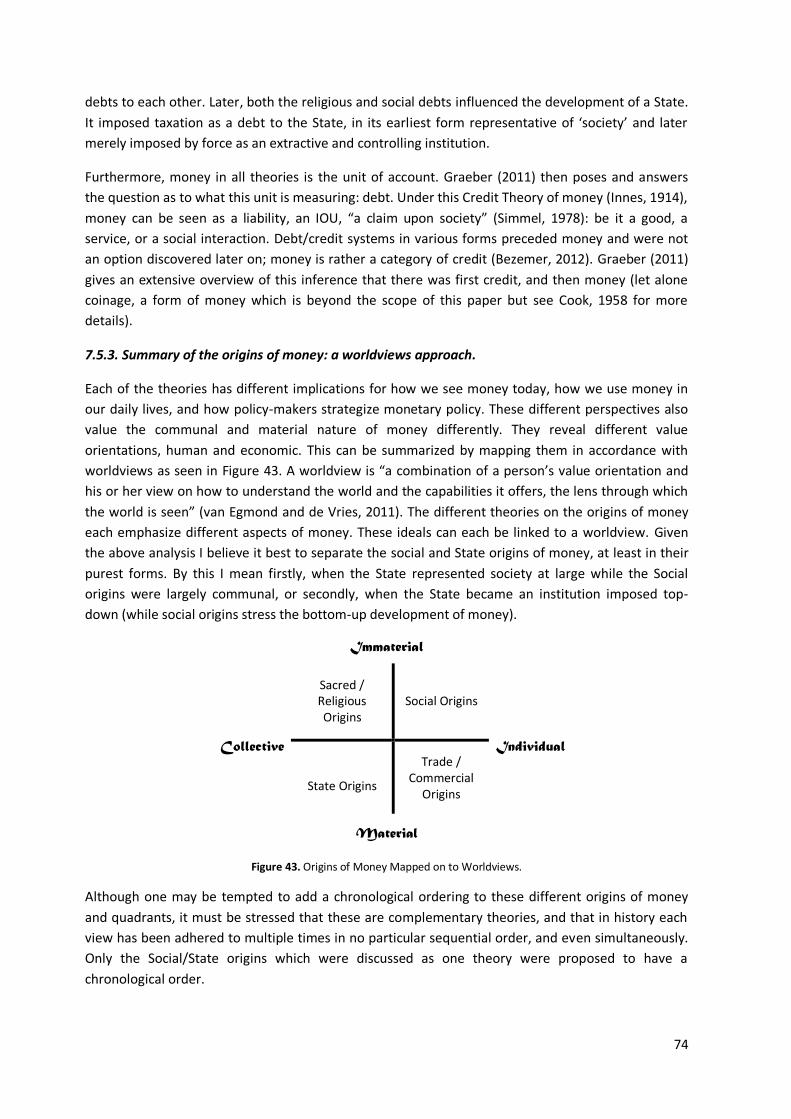
74

debts to each other. Later, both the religious and social debts influenced the development of a State.

It imposed taxation as a debt to the State, in its earliest form representative of ‘society’ and later

merely imposed by force as an extractive and controlling institution.

Furthermore, money in all theories is the unit of account. Graeber (2011) then poses and answers

the question as to what this unit is measuring: debt. Under this Credit Theory of money (Innes, 1914),

money can be seen as a liability, an IOU, “a claim upon society” (Simmel, 1978): be it a good, a

service, or a social interaction. Debt/credit systems in various forms preceded money and were not

an option discovered later on; money is rather a category of credit (Bezemer, 2012). Graeber (2011)

gives an extensive overview of this inference that there was first credit, and then money (let alone

coinage, a form of money which is beyond the scope of this paper but see Cook, 1958 for more

details).

7.5.3. Summary of the origins of money: a worldviews approach.

Each of the theories has different implications for how we see money today, how we use money in

our daily lives, and how policy-makers strategize monetary policy. These different perspectives also

value the communal and material nature of money differently. They reveal different value

orientations, human and economic. This can be summarized by mapping them in accordance with

worldviews as seen in Figure 43. A worldview is “a combination of a person’s value orientation and

his or her view on how to understand the world and the capabilities it offers, the lens through which

the world is seen” (van Egmond and de Vries, 2011). The different theories on the origins of money

each emphasize different aspects of money. These ideals can each be linked to a worldview. Given

the above analysis I believe it best to separate the social and State origins of money, at least in their

purest forms. By this I mean firstly, when the State represented society at large while the Social

origins were largely communal, or secondly, when the State became an institution imposed top-

down (while social origins stress the bottom-up development of money).

Immaterial

Collective

Sacred / Religious Origins

Social Origins

Individual

State Origins

Trade / Commercial

Origins

Material

Figure 43. Origins of Money Mapped on to Worldviews.

Although one may be tempted to add a chronological ordering to these different origins of money

and quadrants, it must be stressed that these are complementary theories, and that in history each

view has been adhered to multiple times in no particular sequential order, and even simultaneously.

Only the Social/State origins which were discussed as one theory were proposed to have a

chronological order.

75

The social origins of money lie in the interaction between individuals at a very communal level.

Concepts such as ´Wergild´ were discussed, and money takes on a role to enable inter-personal

payment and compensation in small communities. This started off largely immaterial, such as

payment for personal injury or marriage. Over time, these social relationships were institutionalized

and one drifts towards the third quadrant. Today, various communities have similarly established

their own money system. Indeed, various proposals for monetary reform lie in this quadrant (see for

example Lietaer, 2001). These proposals stress the need to develop a greater diversity of monies that

have different natures and do not all stimulate material growth and individual enrichment in the way

the current monopolistic currency does. Considering that all the origins have debt in common: debt

to other individuals, debt to God, and debt to society as a whole, this interpretation of money may

reveal a debt to one’s local community. More local money systems such as Local Exchange Trading

Systems (LETS) are proposed in various forms, in an attempt to better fulfill the very different

functions that money has.

In the second and third quadrant lie the State, and sacred / religious theories respectively. Of course,

all money will have commenced locally, but these theories emphasize the institutional, collective

nature of money rather than its use solely between particular individuals. The purely sacred

interpretation is immaterial. Money developed out of a need for a sense of security, as the individual

was overwhelmed by the Other, the world, and thus developed a spiritual world for reassurance. This

is the second quadrant. Only when explicit authorities and formal systems of payment developed this

became more materialistic. This interpretation is associated with progress, and an economic

development approach to society instead of religious. The Charlatist view is the culmination of this

interpretation of money, money owes its value to the State, which it maintains through taxation. It

belongs in the third quadrant. Again, although the Charlatist view is not associated with physical

money, the material aspect can be seen in the provisions of the State for its populace. The two

collective quadrants reflect anthropological evidence, which reveals that monetary units were based

on grains (Wray, 1990) and set equal to a monthly consumption unit (Hudson, 2004b). This means

that the unit of account was not individually optimized in a market process of various private

exchanges as economic market theorists assume, but socially determined according to collective

needs.

The trade and commercial origins of money lie in the fourth quadrant. These result in a private

approach to money, where money is a medium of exchange and thereby does little more than ease

the transactions we make in daily life. Money developed from ambition, as individuals specialized

and diversified their activities. There is a strong bias towards physical commodity money as

promoted by the Metallists. This non-metaphysical, individual approach to money is most influential

today, despite the majority of money not being (related to) a physical item anymore. The material

aspect is found in the market orientation of the trade and commercial origins of money. It reveals

itself today in an ever increasing economic growth, consumption and exploitation as seen in Chapter

3. The market stimulates individual material growth and competition, but as society as a whole

develops, individuals continue to want more to have a more optimal situation relative to others

(Hirsch, 1977).

Today, the diverging interpretations of money are apparent in the introduction of the Euro for

example. Goodhart (1998) presents an interesting analysis of how market versus State origins of

money have different impacts on the implications for the European Union (EU). The common

76

currency was an explicit way to further unite Europe (Risse, 2003), as opposed to the independence

that local or national money generates, but it also had significant commercial benefits. States

attempt to signal unification in various centrally planned ways such as a common language or a

monopolistic currency; however, these efforts frequently fail due to a lack of understanding of the

complexities in the system and ignorance of local situations as well as practical knowledge (Scott,

1998). As the concept of worldviews also points out, we must be weary of such extreme approaches,

which the money system is an example of. Beyond these most simple implications, the social origins

and meaning of money are less explicit in the economic world of today (Klamer and van Dalen, 2000).

Each of these ideals have their limitations and may be better as complementary currencies,

individual, collective, and governmental initiatives that can materialize at different scales as a true

monetary ecosystem (Lietaer et al., 2012). A more integral worldview is required, at the model’s

center that incorporates the various aspects of each quadrant in a sustainable synthesis (van

Egmond and de Vries, 2011). Such an interpretation could yield an understanding of money that is

more diverse, and thereby balances the extremes (i.e. individual-collective and material-immaterial),

accepting and bringing together the different functions of money. The worldview approach helps us

to understand the potential multiple functionality of money as well as the search for a common

understanding. In the debate on the true origins of money, it is most likely that all theories have

something of substance to add to an optimal interpretation of money.

In conclusion, while history has revealed different divergent interpretations of money, its origins

most realistically lie in a gradual convergence of different social practices, religious traditions, and

economic habits over time. Money’s origins lie in the settlement of debts and obligations, be them

private, religious, or State induced. These phenomena do not necessarily exclude each other. Both

Davies (2002) and Graeber (2011) explicitly state this. The variety of different forms of money, times

in history, and locations across the world in which the development of money has taken place also

logically suggest that there is no one all-explanatory factor. In the end, it all depends on how you

define ‘money’, and how you define the theories you investigate.

77

CHAPTER VIII – DEVELOPMENT OF ECONOMIC THEORY, THOUGHT, AND

MODELS OF MONEY

8.1. General Introduction.

Money is a vital ingredient in our current Economy – for wage payments, to pay for the goods and

services we buy, to facilitate investment in new technologies, and to enable specialization and trade.

However, money does not play the same role in theoretical models of the economy. There exist

divergent views on money between modern economic schools of thought. This chapter presents the

development of economic thought on money since the time of Adam Smith. The varying assumptions

that individual schools make, each result in a different role for money in the economy, which is

subsequently reflected in their theories and models. This chapter is organized according to whether

the school of thought finds that:

Money is neutral;

Money is neutral in the long-run, but not in the short-run;

Money is not neutral.

Although there is not a formal chronology in these interpretations, they do generally build on each

other. The assumptions of each model are reduced starting with a basic equilibrative model to more

elaborate ones that attempt to take into consideration more elements and time periods. The role of

money follows from each school’s assumptions. First, there are those theorists whose assumption

that markets equilibrate by price adjustments result in the theory of ‘money neutrality’. These are a

variety of classical economists, ranging from the original classic school of Adam Smith to New

Classical Economics. Neutrality entails that money is a mere intermediary lubricant in the economy

and does not influence its real workings – i.e. what is produced or consumed; neither in the short-

term nor in the long-term. Second, there are Keynesian economists, as well as Monetarists, who find

money to be influential only in the short-term because they assume that prices and wages do not

instantaneously adjust. In the long-term, these adjustments are assumed to automatically occur,

from which follows that money is again neutral. This implies an inherent stability in the system and

that inflation is mainly a monetary phenomenon. Finally, a third school assumes that individuals

cannot reliably predict their future income because of an uncertain future and that not all nominal

magnitudes adjust in price in the long-run (namely, the level of debts do not). These assumptions

yield that money is non-neutral in both the short- and long-term. The main school of thought

associated with this view are Post-Keynesians, although the Austrian school also studies the

influences of money on the real economy in the short- and long-run.

In this chapter, each paradigm is described historically, including the most important economists

associated with it, theoretically by means of a description and the main economic model the theory

is based on, and analytically as to whether their predictions correspond with reality using published

empirical evidence and critiques. Note that simplified models are presented, and there will always be

a discrepancy between how the associated schools of thought judge reality, and what is presented in

the formalized models they utilize. Nevertheless, those presented are considered to be the most

representative of the view. Concluding remarks will summarize the schools of thought in a

chronological overview, and present the preliminary consequences of each view for the research

question of this thesis.

78

8.2. Money has no effect in the short- or long-term on the real economy.

8.2.1. Introduction.

‘Money neutrality’ has been the dominant interpretation of money in Economics, based on the work

of Classical Economics. From the 1970’s this has evolved into New Classical Economics, but the result

that money is of no influence on the real economy remains. This is based on three main assumptions.

First, the assumption that prices are flexible: able to adjust both up- and downwards. Second, it is

assumed that the supply of goods and services will create a demand for these in the aggregate

through the generation of income. Third, the Classics assume household savings equal investment

expenditures in the aggregate, equilibrated through flexible (point 1) interest rates. Behind these

assumptions lies an interpretation of humans as rational economic agents who maximize their known

utility under perfect information. The assumptions imply that markets are competitive and efficient.

They will equilibrate by price adjustments so that any change in the quantity (stock) of money cause

a proportional change in the nominal prices of goods and services (i.e. inflation or deflation), wages

and exchange rates. Real (relative) prices, employment levels, investment, and GDP remain

unchanged (Patinkin, 1987). The increase in both prices and income by the same factor yields no

change in demand; this is known as the homogeneity (of degree zero) in prices of the utility function.

The following section will elaborate upon the advocates of this theory, the terms and theories of the

paradigm, and the main models that are consequentially employed.

8.2.2. Classical Economics.

Classical Economics is one of the first modern schools of economic thought with its roots in the

works of Adam Smith (1776) and David Ricardo (1817), amongst others. The free market is deemed

as an efficient way to allocate resources as markets clear through the adjustment of relative prices

and rational agents that maximize their utility. This yields a self-regulating mechanism, an ‘invisible

hand’, that should be distorted as little as possible in order to function effectively. It follows that

government intervention should be limited to enforcing contracts, property rights, and (perfect)

competition (Ekelund and Hébert, 1990). In addition,

the economy is analyzed from a general equilibrium

(Walras, 1874) and supply-side perspective to which a

corresponding demand naturally exists – Say’s Law

(Skinner, 1967). Classical macroeconomic theory is

based on an aggregation of microeconomic behavior

and the associated assumptions of homo economicus.

Classical theory lays the fundaments of Economics, as

"the study of how men and society choose, with or

without the use of money, to employ scarce productive

resources” (Samuelson, 1955). It follows that money is

neutral with respect to economic outcomes; it is a mere catalyst of exchanges that would have

occurred anyway. This is illustrated with the Quantity Theory of Money. It states that the money

supply has a direct, proportional influence on the price level and thereby results in the money

neutrality denoting that nominal variables do not affect the real sector (Mill, 1848; Lucas, 1996). For

example, if the money supply increases by 10%, the Quantity Theory of Money states that the price

level of goods, services and wages will similarly increase by 10%. No-one’s real income or

Real and nominal factors

A real value takes in to consideration the

change in the general price level over

time. This stands opposite to nominal

values which are not inflation-adjusted.

Nominal factors are prices, wages and

exchange rates. Real factors include the

supply of labor, capital, the state of

technology, output, and employment.

79

expenditures have changed, and therefore neither will demand nor supply. The real sector is thus not

affected by changes in the money supply.

8.2.3. New Classical Economics.

New Classical Economics developed in the 1970’s but remained very similar to the Classics. They

retain a general equilibrium model with perfectly flexible prices, cleared markets, and true prices.

Rational expectations now determine the optimization behavior of individuals; wrong expectations or

voluntary changes in demand and supply can result in temporary economic fluctuations (Barro,

1989). What is important is that decisions are made to maximize utility entirely based on real factors,

giving money a purely enabling function in the economy.

Money neutrality was emphasized quite specifically by various Classics including John Stuart Mill:

"the relations of commodities to one another remain unaltered by money" and "there cannot, in

short, be intrinsically a more insignificant thing, in the economy of society, than money" (Mill, 1871).

The principle has also been denoted as a “veil of money”

(Pigou, 1949). For a more extensive analysis of the

history of the term see Boianovsky (1993). This ‘garb’ or

‘veil’ lies over the economy, enabling it to function, but

with no effect on it. The veil can simply be removed for

economic analyses, focusing purely on the real economy.

Compared to the principle of money neutrality, the

concept of the veil of money relates more strongly to the

question as to whether money is a commodity. Classical

theorists adhere to the commodity nature of money.

This assumption means that money is led by the laws of

demand and supply. Classical theorists also assume the economy is made up of rational agents which

makes the market perfectly efficient; it always clears. An equilibrating demand and supply of money

induces money neutrality in the same way as the Quantity Theory of Money explained. An increase in

the supply of money, will decrease the price of money in terms of other goods, and thereby increase

the nominal price of all goods and services, maintaining equilibrium and leaving the real economy

unaffected. Note that the price of money and the general price level of goods and services in the

economy are each other’s inverse.

8.2.4. A Model.

Many economic models make this assumption, especially in the long run (see next section 8.3): “All

the models we have seen impose long run neutrality of money as a maintained assumption …”

(Blanchard, 1990). The main model utilized is the Fisher model which formalizes the Quantity Theory

of Money as proposed by both Mill (1871) and Hume (1752). Fisher (1911) algebraically presents this

theory with his equation of exchange:

Time periods in Economics

The short run is utilized to denote a

conceptual time period in which some

factors of production (inputs) are fixed,

while in the long run firms can alter their

production as desired. These are not fixed

lengths of time but vary according to the

flexibility of firms.

80

(2)

M = total money stock V = velocity of circulation

P = price level T = number of transactions

This identity states that the total quantity or stock of money multiplied by its velocity of circulation,

equals the price level multiplied by the number of transactions in the economy. Since all transactions

are measured by gross domestic product (GDP), this variable was later substituted for the aggregate

real output (Y) as measured by real GDP.

(3)

The equation assumes that money is necessary to undertake transactions, and that there is a stable

money demand function (T/V or later Y/V). This is based on the idea that velocity of money only

changes very slowly over time and that output is given in the long run by technology and production

factors. Note that as seen in the previous chapter, money is seen to behave here as any commodity,

with a demand, supply, and price. The aforementioned assumptions that the number of transactions

(with output, i.e. GDP as a proxy) and the velocity of money do not depend on the money stock or

price level, yield money neutrality (Humphrey, 1997). Rearranging the identity, and taking into

consideration the stated assumption that there is a stable money demand function, i.e. a constant

Y/V, shows how the Quantity Theory of Money emerges.

(4)

Y/V is exogenous, and thus any increase in the money supply M, must result in an equal increase in

the price level P (when all markets have equilibrated). A doubling of the money supply would double

the price level. In the words of Friedman and Schwartz (1963): “Inflation is always and everywhere a

monetary phenomenon”.

Figure 44 gives a simple illustration of the equilibrating process. If one increases the money supply so

that it is greater than the money demand, people demand more goods in order to sell off this extra

money, resulting in rising prices until equilibrium is restored again. The result of the increase in the

money supply is then an increase in the price level so that the level of real money demand and

Figure 44. Diagram of the Basic Mechanisms of Money Neutrality.

81

demand for goods remains constant. The opposite, a reduction in the money supply clearly has the

opposite sub-effects but the same final outcome of no change in the real quantity of money.

Blanchard’s quote that commenced this paragraph, however continues with: “… This is very much a

matter of faith, based on theoretical considerations rather than on empirical evidence” (Blanchard,

1990). This lack of evidence has resulted in the theories that will follow; these assign more real

power to money, especially in the short-run.

8.3.5. Conclusion.

The Classics have provided the basis of the discipline of economics as is currently being taught.

Notions of money neutrality remain very influential, as it is a useful simplification that eases

modeling efforts. The Fisher equation of exchange is thus also mainly taught for didactic purposes. It

makes analyses such as the task of Central Bankers attempting to control inflation very

straightforward as it implies this can be done by maintaining a certain quantity of money. Over time,

this practice was abandoned in favor of more developed methodologies that could deal with the

complexities of reality that this theory simplifies. The following section considers the limitations of

agents in making transactions for example that this model does not.

Money is neutral because people are rational and perfectly informed which results in market clearing and freely adjusting prices. Subsequently, any change in the money supply is expressed by an equal change in the price level leaving the real economy unchanged.

8.3. Money only has an effect on the real economy in the short-term.

8.3.1. Introduction.

Keynesianism, New Keynesianism and Monetarism make three different assumptions compared to

the Classics. Three main points distinguish Keynesians from the Classics. First, prices are rigid and

inflexible due to a resistance towards wage and price cuts by workers and producers respectively.

Second, demand is driven by actual disposable income and not that at full employment, which is

rarely reached because of the aforementioned rigidities. Third, savings and investments are not

solely a result of the interest rate. Savings are determined by household disposable income and their

demand to save for the future while investments are dependent on expected profitability. Humans

are no longer perfectly rational agents with perfect information – they have bounded rationality. This

entails that there is imperfect information and that the agents undertake biased analyses of this data

because of their cognitive limitations. This limits their capacity to adjust prices of goods and services

immediately and perfectly. The result is a time lag between alterations in the money supply and price

changes, and equilibrating oscillations in the short-term: money non-neutrality.

In terms of the policy implications, this means that in the short-run, monetary policy can affect real

variables. As an aside, Marx also will be considered. Although a classical economist, he fits into this

category because his observations of the economy and related assumptions also yield money non-

neutrality in the short-run. The following section elaborates on these schools of thought, presenting

the main assumptions, principles, and theories of each school as well as some basic policy

implications. Finally, the general model that is utilized by (New) Keynesians and Monetarists is

82

presented in detail, as it more clearly reveals the basic mechanisms that result in money being non-

neutral in the short-run, but neutral in the long-run.

8.3.2. The Keynesian School.

Keynesian Economics is based on the work of John Maynard Keynes (1930, 1936). Keynes attacked

the premise of Classical economics that supply will create its own demand (Say’s Law). Consequently,

markets fail to clear in the short run causing, amongst others, unemployment. Public intervention, in

the form of fiscal or monetary policy, can help to bring the economy to its equilibrium. Keynesians

relaxed some of the assumptions of the Classics. Agents in the economy can be adaptive learners as

opposed to perfectly rational and informed, effective demand is assumed to determine output and

employment, and markets do not necessarily clear because individual decisions may not be optimal

at the macro-level (Eatwell and Milgate, 2011). As a result, money is not neutral in the short-term,

because of sticky wages and because the money supply determines the interest rate. If the money

supply is altered, the interest rate changes and this affects the profitability of investing. This change

in investment, according to Keynesian demand-side Economics, alters aggregate demand and

thereby affects the real economy with a multiplier (Tobin, 1958). In the long-run, it is believed that

these mechanisms stabilize: prices adjust and the economy returns to an equilibrium. However, in

the short-run, there are some fixed factors of production for firms and wages do not adjust

automatically due to contracts; therefore money is non-neutral. Keynes (1930, 1936) laid the

foundation for money non-neutrality. His analyses of the economy included real but also financial

and capital assets which provide income and can be bought or sold to control the associated money.

By being able to store money for an uncertain future, money influences the real economy.

Furthermore, investment in this economy is dependent on the different assets that are invested in,

and their associated flows, as well as financing options. By including the financial sector in the real

economy, Keynes commenced the theoretical trajectory towards money non-neutrality. He did not

build a formal model to demonstrate his arguments, but his ideas were built on more formally by

later economists such as Hicks (1937). The resulting model is discussed below. In sum, Keynes

stressed the monetary nature of the economic system, which inherently allocates a role to money.

8.3.3. The New Keynesian School.

New Keynesian theory builds further on the sticky nature of prices of goods, services, and labor to

attempt to explain unemployment, business cycles, and credit cycles, by analyzing the micro-

foundations of these occurrences (Greenwald and Stiglitz, 1987). It is these rigidities that make

money not neutral in the short-run. Rigidities can be due to the cost of having to change prices:

menu costs, asymmetric demand due to imperfect information, or because producers want to avoid

demand effects as customers may change their consumption pattern when their real income changes

(Mankiw and Romer, 1991). Blinder (1991) presents and tests other reasons. Nominal rigidities such

as sticky prices and wages have also recently been included in standard economic Dynamic Stochastic

General Equilibrium models by (Woodford, 2003) in an attempt to improve monetary policy. New

Keynesians as well as monetarists (see next paragraph) furthermore emphasize the concept of

exogenous money. This defines the amount of broad money in circulation as a function of the money

multiplier (influenced by the reserve ratio) and the amount of high-powered government money in

circulation. By this definition, and as seen later in the model that is used by this school, an increase in

83

high-powered money by the central bank can influence the economy’s output in the short-run

through the interest rate (Friedman and Schwartz, 1963).

8.3.4. Monetarism.

Monetarism is a branch of economic thought that specifically focuses on the effects of the money

supply. Milton Friedman is a key economist in this school of thought. His empirical work on business

cycles in the US revealed that the Classical assumptions associated with money neutrality, for

example that if the quantity of money increases 100 times then it must be that “all other nominal

magnitudes … are also multiplied by 100” (Friedman, 1969), did not correspond with reality. Rather,

the money supply can influence short-term economic activity and inflation because it affects

demand. Excess money can increase the demand for goods and services (of financial assets) in the

short run above the economy’s potential equilibrium output resulting in inflationary pressures (and

vice versa resulting in deflationary pressures). Inflationary or deflationary spirals can result, in which

the expectations of consumers and producers cause a positive feedback. Expectations of economic

growth and the associated higher money supply and inflation induce workers to bargain for higher

wages and firms to increase their prices to avoid the associated inflation costs (Hahn, 1980). Inflation

makes it difficult for firms to plan their investments accurately, resulting in inefficiencies, increased

costs for consumers, and significant redistributive effects. The costs of inflation are also known as an

‘inflation tax’. Deflation, however, also has negative effects. It is caused by a contracted money

supply as experienced for example in the Great Depression, and can lead to postponed expenditure.

In this manner, the money supply, through impacts on expectations and then prices, can have real

output effects in the short-run.

In order to maintain economic stability, monetarists advocate credible control of the money supply

and credit. Credibility is important because of the role of expectations. Friedman (1969) for example

proposes a zero nominal interest rate to limit inflationary and deflationary costs to their socially

optimal level. Government monetary policy is needed to ensure the exogenous supply of money

matches its endogenous demand (Cagan, 1987).

8.3.5. Marx.

As an aside, although considered a classical economist, Marx (1867) also rejected money neutrality in

the short-run but he took a very different approach than (New) Keynesians and monetarists. He

considered the influence that money has on production, and in particular the impact that the

creditors that have to fund this production have. The following quote is included for illustrative

purposes, revealing with which vigor he approached the topic:

“Talk about centralization! The credit system, which has its focus on the so-called national banks and

the big money-lenders and usurers surrounding them, constitutes enormous centralization, and gives

this class of parasites the fabulous power, not only to periodically despoil industrial capitalists, but

also to interfere in actual production in a most dangerous manner – and this gang knows nothing

about production and has nothing to do with it”.

Marx (1894).

Marx also emphasized the social effects of disconnecting money from commodities. He believed the

conviction of the Classics that money was neutral, was a mere method to disguise and encourage the

84

accumulation of money purely for monetary reasons and not for the use of the commodities by

households and firms (Bretton, 1980). His analogy of standard production and consumption is C-M-

C’: a commodity (C) buys another commodity (C’) with money (M). However, this can become M-C-

M’ where money is used to generate more money by means of a single commodity or rather with

capital. This disconnects producers from consumers, and enables individuals to allocate resources

inefficiently purely for monetary gain. In this model, Marx also questions where the surplus M’-M or

C’-C comes from in the M-C-M’ and C-M-C’ analogies. This can be interpreted as extra resource

exploitation resulting in constant environmental degradation and resource depletion, labor

exploitation resulting in increasing inequality, or an increase in productivity through technology. The

role that money plays in this is given his analogy M-C-M’, where M’ > M, suggesting that an economic

surplus, or profits, requires a growing a money supply.

8.3.6. A model.

Mainstream economics today is for the largest part based on Keynesian and Monetarist theory, and

not on Marx. The ‘neo-classical synthesis’ has integrated the varieties of Classical, Keynesian, and

Monetarist thought in the IS/LM model that will be presented in more detail below (Samuelson,

1955; Clark, 1998). The model was first proposed by Hicks (1937), in an article with a title that

already explicitly emphasizes this synthesis: Mr. Keynes and the Classics. It is derived from different

equilibrium output loci in the goods and financial markets, which result from alterations in the

interest rate. Together with the AS-AD model (see below), we can present the view that money is

neutral in the long-run, but does have a short-run effect as follows.

We commence with the goods and financial markets. In the goods market, equilibrium is defined as

the situation in which production or output ( ) equals the demand for goods ( ). Demand is defined

as the sum of consumption ( ), investment ( ), government expenditure ( ), and net exports ( )

which equals exports minus imports. These factors are each dependent on a number of other

variables:

a. Consumer spending ( ) is positively dependent on disposable income (income ( ) minus

taxes ( ) which is in turn dependent on income).

b. Investment spending ( ) is dependent on the level of sales (income ( ), assuming sales

equal production), and the nominal interest rate ( ). The first relation is positive: if a firm

has increased sales it needs to increase production and thus may need additional

machines or plants (investment). The second relation is negative: to undertake such

investment the firm may need to borrow and a higher interest rate makes it less attractive

to borrow. Note that the nominal interest rate is equal to the real interest rate plus

expected inflation.

c. Government spending ( ) is assumed to be exogenously chosen by government.

d. Net exports ( ) increase with income.

Net exports ( ) is dependent on income, and in an extended model also on exchange and interest

rates.

(5)

85

This is equated to output such that:

(6)

The relationship can be described as follows: “Production depends on demand, which depends on

income, which is itself equal to production. An increase in demand, such as an increase in

government spending, leads to an increase in production and a corresponding increase in income.

This increase in income leads to a further increase in demand, which leads to a further increase in

production, and so on. The end result is an increase in output that is larger than the initial shift in

demand, by a factor equal to the multiplier” (Blanchard, 2011). Alternative to this perspective which

considers the production and demand for goods, equilibrium in the goods market can also be found

by focusing on investment and savings. Savings are the sum of private and public savings. Private

savings ( ) are by definition equal to consumer disposable income minus their consumption:

(7)

Public saving is equal to taxes minus government expenditure ( ). Given a closed economy (net

exports = 0), the income equation from above can be rearranged and rewritten for investment as:

(8)

(9)

(10)

Investment spending is thus the sum of private saving and public saving. This equality gives the IS

curve its name: investments equals savings. By altering the interest rate, different demand curves (in

the figure below denoted by ZZ) can be plotted and the IS curve can be derived. An increase in the

interest rate reduces investment and output, which through a multiplier effect further decreases

consumption and investment. This process equilibrates the system to a new lower level of output

and demand as seen in the figure below.

subtract T from both sides

l

recall S = Y – T – C and rearrange

86

Figure 45. Derivation of the IS Curve (Blanchard, 2011).

We see that the IS curve is downward sloping. Equilibrium in the goods market means that an

increase in the real interest rate decreases output. Any changes in factors that decrease (increase)

demand for a given interest rate shift the IS curve left (right). These include an increase in taxes, a

decrease in government spending or in consumer confidence.

In the financial markets, the interest rate is determined by equilibrating the demand ( ) and supply

( ) of money. The supply of money is given by the real money stock (

). The demand for money

depends on liquidity demand ( ). The alternative to holding money is holding bonds so liquidity

demand gives the preference of society to hold cash instead of bonds. These (unlike money), pay a

positive interest rate ( ) but cannot be used to undertake transactions. The demand for money and

bonds depends on the number of transactions you take and the interest rate on the bonds. A higher

level of transactions requires more money, and given the level of transactions is likely to be

proportional to income, greater income requires increases money demand. A higher interest rate

increases the willingness to buy and hold bonds, and decreases the demand for money. The interest

rate is thus the opportunity cost of holding money versus bonds. This yields:

(11)

By plotting a new money demand curve for different income levels, the LM curve can be derived as

seen in the figure below.

87

Figure 46. Derivation of the LM Curve (Blanchard, 2011).

An increase in income, for a given interest rate, increases the demand for money. However, at a fixed

money supply, this increased demand results in an increase in the interest rate. In this process of

equilibration, the increased interest rate acts as an opposing force (reducing money demand) to the

higher income (which increased money demand). A new financial equilibrium is reached when these

two forces cancel each other out. Because an increase in income yields an increase in the interest

rate the LM curve is upward sloping. At a certain level of income, a change in the real money stock

(

) will shift the LM curve: up for a decrease in the money supply and down for an increase in the

money supply.

The IS/LM model combines these two curves on one graph. Any point on the IS curve represents

equilibrium in the goods market while any point on the LM curve represents equilibrium in the

financial markets. At the point of intersection between these two curves both markets are in

equilibrium. The figure below shows this relationship between real interest rates and output when

there is equilibrium in market for goods and services and in the market for money (Figure 47).

Figure 47. The IS/LM curve (Blanchard, 2011).

Based on this short-term relationship between output and interest rates, we can derive a

relationship between output and prices known as the AS-AD model. This stands for aggregate supply

(AS) – aggregate demand (AD). It gives combinations of price levels and quantities of goods produced

at the macro-level in equilibrium. The IS/LM and AS-AD curves all equilibrate simultaneously, at the

same combination of interest rates and output. The AD curve can be derived from the IS/LM model

: nominal money supply : price level : liquidity demand : nominal interest rate : real income : consumption : taxation : government expenditure : investment expenditure : net exports: exports minus imports

88

by plotting LM curves for different price levels and subsequently determining the associated output

as seen below.

Figure 48. Derivation of the AD Curve (Blanchard, 2011).

A higher price level shifts the LM curve up and to the left to an equilibrium point at a higher real

interest rate and lower output. The higher price level can be indicated on a separate graph, together

with the new output level. Connecting these various equilibrium points yields the AD curve. Based on

this, any variable that causes the IS or LM curves to shift, other than a change in price level (i.e. real

money supply, government spending, or taxation), will also cause a shift of the AD curve. A change in

price level will merely cause movement along the AD curve.

The AS curve gives the effects of macro-economic output produced on the general price level. It is

derived from price and wage setting behavior (see Blanchard, 2011). Here the explanation is

restricted to a more general one. Two different AS curves exist: a short- and long-run curve. Since

prices remain fixed in the short-run, the short-run AS curve (SRAS) is horizontal – any quantity has to

be produced at a certain price. In the long-run (LRAS) prices are flexible but the total quantity that

can be produced is limited by fixed technology and factors of production yielding a vertical curve.

This is a situation of full employment (FE).

Money non-neutrality in the short-run, and neutrality in the long-run, can be deduced from this

model as follows. An increase in the nominal money stock (M) shifts the LM curve outward and

moves the economy from point E to point F in Figure 49.

i

89

Figure 49. Short-run Money Non-neutrality, and Long-run Neutrality (Abel, Bernanke and Croushoure, 2010).

The monetary expansion decreases the real interest rate in order to clear the money market,

equilibrating the demand and supply for money. In the goods market, a lower real interest rate

increases investment spending which increases output. A higher output also increases disposable

income for consumers, enhancing the effect. The change in output at this same price level is also

reflected in the AS-AD model, by an outward shift of the AD curve, moving the economy from point E

to point F in Figure 50.

Figure 50. Short-run Money Non-neutrality (Abel, Bernanke and Croushoure, 2010).

The AS-AD model shows that in the short-run the price level does not change. At this new point (F),

output and employment are above their natural level that the LRAS indicates (H), and the price level

is lower than it would be at this natural level. Over time, wage setters respond by revising their

expectations of the price level and thus their wages upwards. Firms in response raise their prices,

also because they have been producing above potential output. This shifts the SRAS curve upwards

moving the economy to point H in Figure 51. Note that although this is shown in the graphs as single

steps, a process of adjustment occurs that takes time and various steps as long as equilibrium output

exceeds the natural level of output because at these points prices still turn out higher than expected.

90

Figure 51. Long-run Money Neutrality (Abel, Bernanke and Croushoure, 2010).

In the long-run output falls back again to its original level in response to the higher price level, as

does the real interest rate. The price level at this point is what would have been expected with the

increased nominal money stock. The increase in the price level is proportional to the increase in

nominal money that initiated the changes. The return back to the original output level is also

reflected in the IS/LM model as seen in the return of the economy to point E in Figure 52.

Figure 52. Long-run Money Neutrality (Abel, Bernanke and Croushoure, 2010).

Again note that in this example the return to the original level of equilibrium occurred in one step.

Usually, the process occurs in multiple adjustments, which continue until the prices have adjusted so

much that the output and the real interest rate have returned to their initial point, and the IS-LM

curves intersect at their initial position of full employment. The timing with which this process of

adjustment occurs is what makes money not neutral in the short-run, although the length of these

periods is not set. An increase in the nominal money supply will initially merely increase output and

decrease real interest rates. Eventually however, the increased money supply will simply result in an

increase in prices and real output nor interest rates are affected.

In sum (see Figure 53), in the short run, a monetary expansion increases output and real interest

rates while prices do not yet adjust. In the long run, an increase in the nominal money supply is

merely seen back in prices, not and not output.

i

91

This long-run money neutrality is also incorporated in the long-run growth Solow model (Solow,

1956). It assumes a fixed savings rate and a set pattern of capital accumulation, and no effect of

money. Tobin (1965) changes this; assuming a demand for money he modeled portfolio decisions

and thereby the effect of inflation on savings and investments. Under high inflation, individuals

substitute their investment towards physical capital instead of financial assets and a higher steady-

state capital stock and output result. Another long-run growth model, the Ramsey (1928) model, has

also been extended to incorporate money by the ‘money-in-the-Utility-function’ which models

money as by definition providing utility by facilitating transactions and thereby reducing the

‘shopping time’ required (Walsh, 1998). With money in the utility functions of households and in the

budget constraint of government, an optimal quantity of money results. However, the model

assumes a direct relationship between money growth and inflation: money neutrality. The details of

these extensions are beyond the scope of this thesis. They merely reveal an attempt to incorporate

money into long-run growth models through various shortcuts, and not with a real long-run effect.

Differences in how money is created or what form it has are not directly considered in the models.

8.3.7. Conclusion.

Keynesians and New-Keynesians recognized the limitations of the Classics and were able to model an

additional part of economic reality that was until then not well understood. Although they maintain

the equilibrative nature of the Classical models, they consider different time periods in which this

adjustment process occurs in order to reveal the effect of money in the short-term. The short-term

non-neutrality of money stems from the fact that factors in the economy do not automatically adjust

to each other, because of various limitations of the market and it’s agents such as imperfect

rationality and information. However, in the long-run, money remains a neutral factor. Furthermore,

although these schools model and explain the non-neutrality of money in the short-run, they do not

consider the nature of money per se to be of influence on this. It is merely the adjustment time that

causes the non-neutrality. The following more heterodox schools of thought find the non-neutrality

of money more in its nature, than in the limitations of market participants.

Money is non-neutral in the short-run because the price level takes time to adjust, but in the long-run this occurs and a change in the money supply leaves the real economy unaffected.

Figure 53. Diagram of the Basic Mechanisms of Money Non-neutrality in the ST, and Neutrality in the LR.

92

8.4. Money has an effect on the real economy in the short- and long-term.

8.4.1. Introduction.

Heterodox economists vary in their assumptions, theories, and models. I will focus here on the

heterodox schools that generally agree that money is created endogenously, and that money is not

neutral in the short-run, nor in the long-run (Wray, 2007). Furthermore, they do not find that the

economy tends to a long-run equilibrium, but that it exhibits long-run cyclical behavior. The Austrian

school and Post-Keynesians find money is non-neutral because they assume that the future is always

uncertain (i.e. future incomes cannot be known) and because not all prices adjust to a change in the

money stock – namely, the level of debts do not. They reject perfect information in favor of there

always being information asymmetry, recognize social, ethical and institutional factors in individual

decision-making, and irrational behavior by agents. Together, this yields that the market’s ability to

equilibrate is extremely limited and even improbably both in the short- and long-run. In terms of

money, not only can the quantity of money then have an effect on the real economy, but so does the

way in which this quantity is supplied (money creation), and the form which money takes in the

economy. For example, differences between central bank (deposits) and commercial bank money are

more explicitly examined, the form of money is distinguished from it as liquidity or a unit of account

in monetary analyses, and the effect of money as debt is studied. By specifically acknowledging the

existence of money, with a wide variety of interpretations, these theories claim to make more

realistic assumptions and thus predict economic outcomes better (Keen, 2012a).

Austrian Business Cycle Theory is the starting point of most analyses of money in the Austrian school.

A large portion of the literature focuses on the negative effects of ‘fractional reserve banking’, their

analysis of how money is created. Post-Keynesians commence from the observation that banks

control the money supply by means of interest-bearing credit creation, and investigate the effects on

the real economy from there. Their name refers to their view that Keynes has been largely

misinterpreted in the past. They depart from Keynes’ understanding that there was a large difference

between the classical “real exchange economies” and “monetary economies” (Keynes, 1933) where

banks can expand the money supply, and his observation that “credit expansion provides not an

alternative to increased saving but a necessary preparation for it. It is the parent, not the twin of

increased saving” (Keynes, 1939). Few economists grasp the repercussions of interpreting the money

system as such. Post-Keynesians find that such observations and logic have been largely lost, and

attempt to reintroduce these into economics. A third school of thought that considers the effects of

money is less considered in the West: Islamic Economics. They have historically (like various other

religions also – Christianity, Judaism), been concerned with the effect of interest on society, and thus

today with the form in which our money is created – as interest-bearing debt.

This section will present these schools of thought in terms of some important academics within

them, and their main ideas. These heterodox theories have been largely developed in the 20th

century, and are not widespread in textbooks. Unlike the Classical and Keynesian schools, they do

not have a general theory and model of the Economy. Nevertheless, abstract models will be

presented in an attempt to depict the assumptions of these schools. This final section is a useful

transition to Chapter 9 on the workings of our current money system, which are most closely studied

by this group of Economists.

93

8.4.2. The Austrian School.

The Austrian school has, although established by quite traditional money theorists such as Menger

(recall the previous chapter), grown to consider the effects of money in the economy quite explicitly.

The Austrian school, like the Classical school, assumes the price mechanism can organize the market

best without any government intervention beyond ensuring strong property rights and contracts

(Hazlitt, 2011). However, it differs from Classical as well as Keynesian schools in that it judges human

behavior too complex and unique to mathematically model accurately or usefully and thus does not

make claims based on such models. The Austrian school rejects the previously described Classical

idea that money is solely a numeraire. They also explicitly consider the effects of changes in the

money supply on the basic decisions of individuals. Mises (1934) incorporated monetary theory into

economics in his 1912 Theory of Money and Credit. He introduced important topics which are later

developed further by other Austrian Economists including Austrian Business Cycle Theory, fractional

reserve banking, and the optimum quantity of money in relation to money non-neutrality and price

instability (North, 2012). Mises also described the origins and definition of money as a means of

exchange based on work by Menger and Jevons (recall Chapter 4). Money is assumed to exhibit

diminishing marginal utility like any commodity. This is determined by the purchasing power of

money, both now and in the future. This varies significantly because valuation is done by subjective

and unpredictable individuals. An increase in the stock of money will have significant redistributive

effects due to this variation, as well as due to the fact that the first person to receive any newly

created additional money can buy goods at still unaffected prices (Ekelund and Hérbert, 1990).

Money thereby concentrates wealth with those closest to the point of creation, at the expense of

individuals further away, those who do not receive credit, and people on fixed incomes.

Austrian Business Cycle Theory was further developed by Hayek (1967). Ekelund and Hérbert (1990)

and Keeler (2001) describe this theory as follows. An unexpected increase in the money supply

increases the amount of loanable funds (excess credit creation) which decreases the interest rate.

Austrian theorists claim this is often aggravated by central bank policies who maintain too low

interest rates, and the fact that the money supply can be further expanded through fractional

reserve banking (see below). In equilibrium, the interest rate equals the rate of return on capital

(rate of marginal productivity of capital), but the lower interest rate disrupts that equilibrium. The

interest rate is now lower than the return on capital, which alters the returns to investments and the

structure of production. Resources are reallocated to capital investments as in relative terms this

investment is cheaper than investments closer to the production of final consumer goods. The

overinvestment in capital goods alters the capital stock. Since most capital goods have long lifetimes,

and since most capital investment decisions are irreversible, the effect of the change in resource

allocation on the economy is visible in the long-run. Physical lags in the economy because production

takes time and because capital has a lifetime, as well as limited information and bounded rationality

of the economic agents result in these imbalances which produce the long-term effect that we see as

the business cycle.

The expansionary cycles rely upon an excessive increase in the money stock. This is closely related to

the issue of fractional reserve banking as it enables such an expansion. Fractional reserve banking

entails that banks only have to hold a specific portion of their deposits and can lend what they do not

have to keep in reserve out to borrowers. This portion is known as the reserve ratio. Fractional

reserve banking increases the money supply enabling more access to credit, but also creates the

94

possibility of a bank run since a bank will never have the total amount of deposits in its possession.

One is reminded of the ‘animal spirits’ that Keynes used to describe the “spontaneous urge to action

rather than inaction, and not as the outcome of a weighted average of quantitative benefits

multiplied by quantitative probabilities” (Keynes, 1936). He explained how this determines the

confidence of individuals in the market and because of irrationality results in a second source of

instability in financial markets following speculation. Austrian school Economists generally oppose

the idea of a reserve ratio as it adds an exogenous, fallible control over the money supply. Too much

or too little creation will result in artificially low or high interest rates which always return to their

natural level, thus creating a boom and bust cycle in which resources are allocated differently (Block

and Garschina, 1996).

The critique of the Austrian school to the way fractional reserve banking currently functions reveals

itself in two opposing views. The first is in favor of less regulation of money creation and no limits to

reserves, while the second advocates more regulation, and a higher reserve ratio. Hayek for example

proposes to denationalize money (1976) and allow anyone to create it. Free trade and competition in

money and banking discipline issuers and stabilize the money system (limited

appreciation/depreciation) as only the ‘best monies’ (with stable purchasing power) would survive.

This free banking system would have a decentralized financial system, with no central bank nor

government intervention setting rules concerning reserve ratios. There would be full private money

creation and currency competition. In this extremely liberal approach, the public sector in this sense

is not the solution, but actually the reason of instability. Although this theory has been largely

dismissed on the basis of the existence of market failures, strong network externalities, and path

dependencies, it is regaining interest and there is even some historical evidence that it may work. In

the 19th century, there was free banking in the United States allowing basically anyone to issue their

own bank notes from commercial banks to firms to individuals creating a confusing and elaborate

money system (Galbraith, 1975). In 1836 the Coinage Act was passed which required government

payments to be made in gold or silver, eliminating the ability to pay with commercial bank notes; a

panic ensued (Galbraith, 1975). This may indicate a certain stability that the previous system

ensured; indeed free banking was subsequently reinstated until 1866. In England, private coins were

issued by The Parys Mine Company and the Soho mint in a period of shortage of small change,

ensuring the industrial expansion in the 1700s could continue (Selgin, 2010). The costs and benefits

of such a system in the complicated, and globalized world of today remain to be judged.

The opposite view is described by another Austrian economist, Rothbard who desired to eliminate

the fractional reserve banking system because:

“issuing promises to pay on demand in excess of the amount on hand is simply fraud, and should be

so considered by the legal system. For this means that a bank issues "fake" warehouse receipts--

warehouse receipts, for example, for ounces of gold that do not actually exist in the vaults. This is

legalized counterfeiting; this is the creation of money without the necessity for production, to

compete for resources against those who have produced . . . . I believe that fractional reserve banking

is disastrous both for the morality and for the fundamental bases and institutions of the market

economy”

(Rothbard, 1991).

95

Rothbard proposes full (100%) reserve banking, a proposal that has been taken up by various

academics, also from the Classical school. See for example Fisher (1936) and Friedman (1960), who

claim this would eliminate the need for the central bank as a lender of last resort in cases of crisis.

See for a judicial and historical perspective Austrian economist de Soto (2009).

8.4.3. The Post-Keynesian School.

Post-Keynesians take a critical position similar to Rothbard; however derive this from very different

observations. The principle of fractional reserve banking is namely rejected, as Post-Keynesians claim

that banks are not limited by their reserves when making a loan – they can make the loan, and find

the reserves only afterwards (Holmes, 1969; Moore, 1983). The time lag that arises between having

the reserves one needs for a loan, has in recent decades been extended from two weeks to a month

(Keen, 2012a). Post-Keynesians claim that when a loan is extended, a deposit is simultaneously

created, which can enter the economy to be used as ‘money’. Therefore, “though it may appear that

the state controls the money supply, the complex chain of causation in the finance sector actually

works backwards” (Keen, 2011). This principle is denoted as endogenous money creation, as the

market, including and via commercial banks, determines the money supply. This process will be

further discussed in Chapter 9. Important is that the Post-Keynesian school rejects a number of key

Classical and Keynesian economic assumptions (see Keen, 2011 for an elaborate critique). This

includes the IS/LM based model of the money supply, the idea of a money multiplier and the

influence of the reserve ratio, the assumption of perfect credit worthiness, and the origins and

evolution of money (Goodhart, 2009). They namely reject the assumption that markets clear in the

long-run due to price adjustments, claiming that not all prices will adjust. While the nominal price of

goods and services may adjust with an increase in the money supply, the nominal magnitude of pre-

contracted debts do not (Keen, 2009b). They also reject the assumption that rational expectations

make future incomes known, assuming rather that the future is always uncertain. By altering these

assumptions, there is no constant linear relationship between the quantity of money and prices that

the models of the Classics and Keynesians rely on.

Unlike mainstream economists, Post-Keynesians purposely include the financial sector as a profit

seeking sector in models of the economy which gives money a non-neutral role in it. Post-Keynesians

recognize that in the current credit economy, there is a necessary task for banks as a third party in

payments and a given ability to extend loans which directly creates (bank) money (Keen, 2009b).

They assign a growth-enhancing role to banks through this process, because new money (credit) is

required to enable investments, which induce growth. As Domar (1957) states: “It is not sufficient…

that savings of yesterday be invested today, or, as it is often expressed, that investment offset

savings. Investment today must always exceed the savings of yesterday…. An injection of new

money… must take place every day” for economic growth. Rochon and Rossi (2004) similarly state

that “In a monetary economy of production, credit is needed to enable firms to continue and expand

production. There is a definitive link between bank credit and economic growth”. Post-Keynesians

argue that while credit is therefore needed for an economy to prosper, one must also consider the

flip-side of credit, which is debt, in analyzing the economy.

Combining the bank’s profit-seeking nature and its ability to expand the money supply through

interest-bearing loans ex nihilo, Post-Keynesians find that there is an incentive for banks to increase

the money supply through increased credit creation in order to maximize profits. To be able to do so,

96

debts for speculative purposes are encouraged as Galbraith (1975) notes: “the banking system, as it

operated in the last century and after, was well designed to expand the supply of money as

speculation required … A healthy bank is making loans and, in consequence, creating deposits that, in

turn, are money”. However, if a bank fails, when for example speculative expectations are not met,

this is not like any business failure. A bank failure is complemented by a contraction in loans,

deposits, and the money supply. Debt and its counterpart credit therefore play an important role in

Post-Keynesian money non-neutrality. The exact mechanisms by which this occurs are considered in

the next chapter.

Minsky developed this in his financial instability hypothesis (Minsky, 1982, 1986, 1992) to explain the

business cycle and the emergence of economic depression. He describes how initially banks are risk

averse in their lending which means most loans are recovered and the related investments succeed.

This makes them more optimistic and they become increasingly willing to lend and less conservative,

earning profits on expanding the amount of credit created while simultaneously stimulating

economic growth. While this boom lasts, it is self-enhancing, trade in debt as well as asset prices

increase with increased demand and the optimism is complemented by a reduction in both

regulation and expensive buffers (van Zanden, 2009). It is also self-validating as increased demand

for assets yields increased prices which enables extra lending. Other parties such as investors,

depositors, and capital owners are also not a limiting force because they too have profit expectations

in this boom. Interest rates rise as there is an increased demand for money (debt), but this does not

stop the boom because asset price expectations far exceed these percentage point changes. There is

a general feeling that unlike previous growth periods that may have led to a collapse, ‘this time is

different’ (Reinhart and Rogoff, 2008).

Increasing levels of debt (credit) in such euphoric boom times lead to speculative and Ponzi finance

as borrowed money is used to gamble on the rising asset prices. Speculative finance entails that debt

can be serviced with current income but that the principal cannot be repaid; in Ponzi finance neither

the interest nor the principal can be paid without new debt. The financial sector takes up a significant

share of the economy altering the system towards ´money manager capitalism´. This entails that “the

proximate owners of a vast proportion of financial instruments are mutual and pension funds. The

total return on the portfolio is the only criterion used for judging the performance of the managers of

these funds, which translates in an emphasis upon the bottom line in the management of business

organizations” (Minsky, 1996). Today, alternative investors such as hedge and private equity funds

have also gained a significant share of financial wealth (McKinsey Global Institute, 2011). These

trends increase the instability of the system further even though they do not create money. Indeed,

when the rising interest costs of debts become greater than income streams these can no longer be

serviced or repaid without selling assets. This reduces asset prices and can lead to a fire-sale of assets

further depressing their price level. Defaults occur, and credit availability decreases, which worsens

the situation. This ultimately leads to a bust: the ´Minsky moment´. The resulting debt-induced

depression is characterized by deflation, high unemployment, low or negative economic growth

rates, low wage and profit rates, and a high income share of the financial sector (see Keen, 2010b for

a model). A psychological component (pessimism), and the impossibility of servicing the debt with

current income can cause the entire bubble to collapse. By considering the debt (credit) nature of

money, and the role of the profit-seeking financial sector in supplying this credit, which responds to

profit-seeking economic agents, money obtains a non-neutral role in the real economy (Minsky,

97

1993). It alters the distribution of income and wealth, has long-term effects on economic growth, and

subsequently on economic variables such as employment.

Government intervention is needed to stabilize these effects and overcome the procyclicality that

was set in motion (van Zanden, 2009). Such intervention needs to specifically monitor debt/credit

levels as these determine the demand for money and subsequently the money supply which in Post-

Keynesian analysis is an important variable in real economic analyses (Bezemer, 2009; Keen, 2011).

An abstract model of the general influence of money of the Austrian and Post-Keynesian school is

seen in Figure 54. This theory “takes banking seriously as a profit-seeking activity” (Minsky, 1992),

where financial innovation, credit creation, speculation, and manipulation cause money to have an

effect on the real economy. More fundamentally, the nature of money as interest-bearing bank debt,

of which the nominal price does not always adjust in the long-run, makes money non-neutral.

8.4.4. Islamic Economics.

Finally, Islamic Economics is based on behavioral norms and interprets money non-neutrality through

its core standpoint on interest which is believed to have an unjust redistribution effect from the poor

to the rich and negative attitudinal effects stimulating selfishness and materialism (Kuran, 1986). The

Islamic banking system is therefore interest free, and rather a small share of the profits created by

means of the loan is shared with the creditor thereby more equally sharing the risk. Meera and

Larbani (2009) present an argument against the creation of money through fractional reserve

banking as this is “creation of purchasing power out of nothing which brings about unjust ownership

transfers of assets in the economy, to the bank effectively, paid for by the whole economy through

inflation”. This inflation tax, as introduced also previously, benefits those that are closest to the point

of money creation as the inflationary effects of the additional money supply have not yet resulted as

the money has not circulated enough and thereby only impairs those furthest (Friedman, 1971). The

‘creation of money out of nothing’ in the form of credit also creates ownership ‘out of nothing’

without work and fair risks. Banks should be rewarded for the risks their stock owners take, for

example with their money, but not for risks they do not assume because society as a whole pays for

this through the mentioned inflation. Chapra (1985) also condemns the distributive effects of

inflation as “it tends to pervert values, rewarding speculation (discouraged by Islam) at the expense

of productive activity (encouraged by Islam) and intensifying inequalities of income distribution

(condemned by Islam)”.

Figure 54. Diagram of the Basic Mechanisms of Money Non-Neutrality.

98

These outcomes conflict with Islamic principles of ownership and prohibition of interest. Islamic

Economists thus aim to develop alternatives to this system: a financial system and money (creation)

that enhances society’s welfare as a whole. Anwar (1987) discusses a variety of options including

nationalization of money creation, the banking system, or 100% reserve requirements but critiques

these for imposing too large rigidities and inefficiencies. Instead, a dual banking system is proposed

that separates private and social banks thereby emphasizing two different needs: saving and

investing. This brings us close to current economic thought where similar proposals to separate the

banking system are reemerging once again through for example a renewed Glass-Steagall (ICB,

2011).

8.4.5. Conclusion.

In conclusion, across the world there are heterodox schools of economics that emphasize that there

are effects of money on the macro-economy in both the short- and long-term. These argue that

there is no constant linear relationship between the quantity of money and prices upon which both

the Classics (Fisher equation) and Keynesians (IS/LM – AD/AS model) rely because the value and level

of debts do not adjust to restore the economy to its natural equilibrium. These effects translate to

the long-term, as the magnitude of nominal debts are not prone to adjustment and the capital stock

in which was invested in the short-run has a long lifetime. While largely absent in Classical and

Keynesian economics, it is then also the role of debt, and in particular of credit, in the macro-

economy, that these heterodox schools emphasize. By focusing on the fact that the money supply is

determined by the credit creation process, the Austrian and Post-Keynesian schools are also able to

explain the pro-cyclical movement of the money supply in the business cycle.

In addition to these purely economic arguments, these heterodox theories also allocate an important

interpersonal effect of money. Money is not just something of the individual consumer as is the

prevailing view in liberal economics but has distributive and social effects. Interestingly, Post-

Keynesians and the Austrians come to the same objection against money non-neutrality but from

very different assumptions and ideologies as seen in their proposed solutions: the former desire

more government intervention while the latter strive for a complete extraction of the government

and central bank from monetary influence. Nevertheless, both make us weary of the impacts of our

money system on the real economy, in the short-run, and in the long-run. Islamic Economics shares

this awareness, from a more normative perspective than the Post-Keynesians and Austrians. The

economy does not tend to equilibrium, it rather exhibits long-run cycles, causing instability and

redistributions of resources in the real economy.

Money is non-neutral in both short-run and long-run because it is bank debt, limiting the capacity of price adjustments to restore the economy to its natural equilibrium and giving money a

pro-cyclical role in the business cycle and economic growth.

99

8.5. Conclusion and discussion.

There is a clear differentiation between the first two theories on money and the third. The former

focus predominantly on whether the money supply has an effect on the main variables of the real

economy – unemployment, output and inflation, and the latter also focuses specifically on the nature

of this money supply. Furthermore, it is only the third school of thought that considers any long-term

steering effects of money. Despite its denotation as Post-Keynesian, it is then important to

distinguish it from the neo-classical synthesis of the Classics and Keynesians. Recall that variations of

Classical Economics maintain the view that money is neutral, merely a veil over the real economy

that does not have any effects beyond ensuring real exchanges occur smoothly. The different forms

of Keynesian Economics, as well as Monetarism, find that money definitely does have an effect on

the real economy, but mainly in the short-run where prices have not had the time to adjust. These

two schools of thought, however, do not delve deeper into how the money is supplied and what

form it takes, while Austrian economists, Post-Keynesians, and Islamic economists have in common

that they all do take this into consideration in their economic analyses. These latter schools focus

their economic analysis on long-term and complex cyclical tendencies of the real economy, which

they claim cannot be modeled or predicted with the Classical equilibrative and linear approach to

economics.

100

CHAPTER IX – THE CURRENT MONEY SY STEM

9.1. General Introduction.

The previous three chapters have laid the foundations for an analysis of how the current money

system functions. A few main conceptual changes have occurred over time that have resulted in

today’s understanding of the role of money in the economy. The origins of money seem to lie in

transferable debts (credits), recorded in accounts (Graeber, 2011). Over time, various forms of

primitive money were used to signify these individual debts. These included commodities, tokens,

currencies, and the official coinage of authorities (Davies, 2002). In the course of history, there have

been various transitions back and forth between such physical money and money as mere accounts

and notes of debts. With the rise of money lending and changing, fractional reserve commercial

banking, and the goldsmiths in the Renaissance, there developed private institutions that had the

power of money creation (Zarlenga, 2002). The debt and credit accounts with these parties were

used as money, enabling transactions irrespective of one’s geographic location and proof of promises

of payment circulated as a medium of exchange. Since, there have been various struggles between

the public and private sector over the power to create money (Zarlenga, 2002). In most OECD

countries, private banks create the majority of money in circulation.

There have also been changes over time in economic theory. The assumptions made by different

schools of thought yield different results for the role of money in the economy. Perfectly rational and

informed agents, together with instantaneously adjusting prices make money a mere neutral means

of transaction, while time lags and bounded rationality give it the power to alter economic activity in

the short-run. As money increasingly dominates society, it is also being considered more specifically

in economics, though until now in mainly heterodox schools. These schools specifically investigate

the nature of money, and argue that since the money we utilize is private, interest-bearing,

commercial bank debt, debt plays an important role in the economy and its nature (nominal level

does not always adjust) makes money non-neutral.

There still exist many misconceptions of money, such as that money is backed by ‘something’ such as

gold or silver, or that it is created by the government. I here present the results of an investigation

into the creation of money – in what form is it created, and how is brought into circulation. A

theoretical section on commercial and central bank balance sheets first provides the basic

understanding needed for the following two subsections because the money creation process in our

current money system is largely based on bookkeeping entries. Equipped with this knowledge, we

explore the process of money creation.

I investigate the role of the central bank and commercial banks in the money supply, the nature of

money as ‘fiat’ money created out of nothing, and the role of debt or credit with associated interest

in this process (Lietaer, 2001). It is especially the latter two characteristics of money creation that are

claimed by critics of the current money system (see the Introduction) to yield unsustainable

outcomes. To determine whether this indeed is the nature of our current money system, various

insights of the money creation process are investigated. Tobin (1963) defined a ‘new’ view on money

creation based on work by Gurley and Shaw (1960), in contrast to the ‘old’ traditional view that is

based on the money multiplier. The new view has recently been rediscovered by Moore (1979, 1983,

1994) and further developed by the Post-Keynesian school, Circuitists, and Modern Monetary

101

Theorists (Wray, 1998; Godley, 1999; Bellofiore et al., 2000; Graziani, 2003; Rochon, 2005; Keen,

2011). Following the accounting basics, I first present the old view in order to obtain an

understanding of the change in perspective that the new view offers. These heterodox theories

consider the role of money in the economy more explicitly, as already introduced in the previous

chapter. The effects of including money in the economy in this manner are considered in Part III.

9.2. Commercial and central bank balance sheets.

The balance sheets of commercial banks and the central bank are closely related to what money is,

and how it is brought into circulation. The discussions in Chapter 6 about what money is can be

clarified by defining it as a mere claim on goods and services in the real economy, as stated, a liability

on the balance sheet of commercial or central banks. In fact, our money today for all practical

purposes (97% according to Dyson et al., 2010), is a bookkeeping entry on a private bank’s balance

sheet only. The amount on deposit, a liability of the bank, only exists in the banks. This extends risks

to the bank such as bankruptcy, insolvability, and illiquidity to the public who has deposited money

there. This thus goes beyond savings, but includes mere transaction accounts.

This section presents the basic accounting equation that is associated with a balance sheet, the

components of commercial bank balance sheet, and of the central bank’s balance sheet. A bank’s

balance sheet is different from a firm’s balance sheet, which produces actual goods and services,

requiring physical inputs to do so. Adjustments in a firm’s balance sheet generally requires real

production, although it also undertakes various purely financial transactions. What it cannot do

though, is expand its balance sheet (assets and liabilities), in the way that a bank does, by simply

creating a loan: it cannot create value ‘out of nothing’. For a bank however, altering its balance sheet

is its ‘production’ and the non-physical nature of their balance sheet makes it easier to alter it in

order to maximize its profits. This in turn affects those parties that the bank deals with. The way in

which the items on a bank’s balance sheet appear on that of individuals and central banks will

therefore also be presented. This will provide a better understanding of how various important

concepts such as deposits and loans are accounted for.

A balance sheet denotes the state of an organization’s financial condition at a particular point in

time. It has a left- and a right-hand side, which must always balance, they must be equal. On the left

are the assets of a firm, and on the right the liabilities and its net worth (also known as its net assets,

capital or owner’s equity). The assets of a bank are what it owns, while it owes its liabilities to

another party (obligations). This can be for example the central bank, government, other commercial

banks, firms, or individuals. The net worth is what balances the equation, it is what would be left if

the bank sold all its assets and paid its liabilities. The net worth belongs to the owners of the bank.

The basic accounting equation linking these concepts is thus:

(12)

Put simply, a bank’s business is to use its liabilities to obtain assets on or with which it makes money.

To maximize profits, it needs to obtain the highest paying assets, by means of the cheapest liabilities.

Liabilities include the owner’s own capital, but also various other loans and through these they can

leverage their position and reduce costs compared to a situation in which they only use owner’s

equity. For illustrative purposes, Figure 55 gives the degree to which major US and European ‘Large

Complex Financial Institutions’ (LCFIs), and UK banks, were leveraged between 2007 and 2011. The

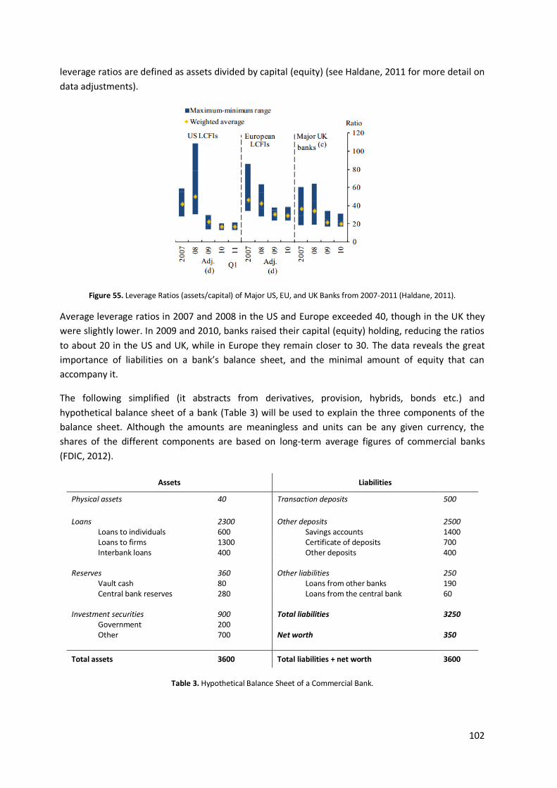
102

leverage ratios are defined as assets divided by capital (equity) (see Haldane, 2011 for more detail on

data adjustments).

Figure 55. Leverage Ratios (assets/capital) of Major US, EU, and UK Banks from 2007-2011 (Haldane, 2011).

Average leverage ratios in 2007 and 2008 in the US and Europe exceeded 40, though in the UK they

were slightly lower. In 2009 and 2010, banks raised their capital (equity) holding, reducing the ratios

to about 20 in the US and UK, while in Europe they remain closer to 30. The data reveals the great

importance of liabilities on a bank’s balance sheet, and the minimal amount of equity that can

accompany it.

The following simplified (it abstracts from derivatives, provision, hybrids, bonds etc.) and

hypothetical balance sheet of a bank (Table 3) will be used to explain the three components of the

balance sheet. Although the amounts are meaningless and units can be any given currency, the

shares of the different components are based on long-term average figures of commercial banks

(FDIC, 2012).

Assets Liabilities

Physical assets 40 Transaction deposits 500

Loans 2300 Other deposits 2500

Loans to individuals 600 Savings accounts 1400 Loans to firms 1300 Certificate of deposits 700 Interbank loans 400 Other deposits 400

Reserves 360 Other liabilities 250

Vault cash 80 Loans from other banks 190 Central bank reserves 280 Loans from the central bank 60

Investment securities 900 Total liabilities 3250

Government 200 Other 700 Net worth 350

Total assets 3600 Total liabilities + net worth 3600

Table 3. Hypothetical Balance Sheet of a Commercial Bank.

103

The left-hand side of the bank’s balance is what is owns: its assets. Firstly, the physical assets of a

bank include its building, office equipment, any land it owns, and any physical capital it may own to

lease for example. This is a minor share of a bank’s balance sheet. Loans, secondly, are the most

important asset of a bank, and on which they earn their revenues through interest payments.

Individuals, firms, or other banks may be borrowers, for whom the loan is a liability. There are a large

variety of types of loans. Part I revealed that an increasing portion of loans is being used for financial

purposes, for mortgages or real estate development. Loans to other financial institutions (interbank

lending) may also be given so that these have enough reserves. Reserves have to be held by banks to

ensure daily transactions function smoothly. The next section will consider this third asset category in

more detail. A bank has such reserves in their vault in the form of cash (part of M0) in order to satisfy

cash demands through ATMs for example, and merely as an account at the central bank to ease

interbank payments. Fourthly, the bank owns investment securities. These may be bought from a

government (national, municipal, etc.), who require funds. As of 2007, other asset-backed securities

and derivatives made up a large portion of these investment securities. This makes the bank’s total

assets vulnerable to changes in the market, as the value of these securities will change depending on

the market price they can receive. This vulnerability depends on whether assets are accounted for on

the balance in terms of their real current market value (mark to market / ‘fair’ value accounting) or

their historical cost which extrapolates from market fluctuations.

In addition, the assets of a bank vary in accessibility, safety, and price. Reserves are the safest assets

as banks have direct access to these. Loans are less safe than investment securities, as there is a

chance that they cannot be paid back by the borrower. Note however that investment securities are

often created on the basis of actual loans, but by combining these and selling them on, the liquidity

of the security becomes greater than that of the individual loan. In theory, securities are easily sold in

the market if needed. Liquidity being the ease with which it can be bought, sold, or converted to

cash. Investment in a more liquid asset or security is safer (less risky) than in a less liquid one because

it is easier to retrieve one’s money. Reserves that are directly accessible are liquid, while most loans

have a certain lifetime and less liquidity; the money is simply not accessible for the bank for a period

of time. Investment securities lie in between the two. There is also a relation in terms of how

expensive each type of asset is: a lower risk reduces the return. Reserves are expensive as they do

not pay interest, the bank even has to pay the central bank interest to obtain them. Investment

securities are safer and pay more interest, but less interest than loans do.

The liabilities of a bank are what it owes. Firstly, transaction deposits are checking accounts owed to

the bank’s customers. For them, the accounts are assets, and the customers can access these at will.

Banks generally do not pay interest on checking accounts and thus these are an inexpensive liability

for the bank. In terms of the money aggregates described above, these accounts are a component of

M1. Secondly, other deposits are less liquid and are part of M2 and M3; these include, amongst

others, savings accounts, certificate of deposits, repurchase agreements, and money market

deposits. These are borrowed by the bank from individuals and firms who therefore do not use them

for payments; they rather receive interest on them from the bank. Note that most people are not

aware that the bank thus actually owns their deposits, whether M1, M2 or M3 (ICM, 2010). These

deposits (mainly M1) are insured to a certain degree, nationally by the government through a State

guarantee or privately (Demirgüç‐Kunt, A. and T. Sobaci, 2001). In addition, the bank may borrow

from the government and other banks. This third category of liabilities includes overnight loans from

other banks to maintain adequate reserves. For example, banks in rural areas may have deficient

104

reserves while those in a large city may have excessive reserves. Lending can overcome this

imbalance, but it requires trust between the banks that the loans can and will be repaid. Banks may

also lend from the central bank for this reason, though this in general is a more expensive liability

(note that at the moment the central bank’s rates are actually very low). Banks also lend money from

other financial institutions such as pension funds or insurance companies. However, this is usually

done by means of a repurchase agreement in which the lending bank gives the borrowing institution

collateral such as a government security.

The difference between the assets and the liabilities is the net worth of the bank. This is the owner or

shareholder’s equity. The owners of the bank have a positive net worth if the assets are greater than

liabilities, and a negative net worth if its liabilities are greater than its assets. The latter situation

entails bankruptcy. In order to avoid this situation, capital adequacy requirements of a bank (ratio of

the amount of net worth they have to have compared to their assets) are established by regulators.

Banks thus need enough net worth to deal with defaults. In normal times, this buffer should be

enough to avoid a situation of negative net worth and hereby the need to reduce deposits.

A hypothetical and simplified central bank balance sheet is presented in Table 4.

Assets Liabilities

Gold and foreign exchange 100 Currency 200

Held by the public 120 Credit 800 Vault cash 80

Loans to banks 600 Government

securities 200

Commercial bank deposits at the central bank

280

Other 430 Government Accounts 250

Other 500

Total liabilities 1230 Net worth 100

Total assets 1330 Total liabilities + net worth 1330

Table 4. Hypothetical Balance Sheet of a Central Bank.

A central bank’s assets include any gold holdings, foreign exchange it has, and credits it has

outstanding. This includes loans to commercial banks as well as government securities which it could

sell. The central bank’s liabilities include the currency that is held by the public, or in the form of

vault cash with commercial banks. Furthermore, the central bank ‘owes’ commercial banks any

deposits they have at the central bank, and it ‘owes’ the government any money it has deposited in

its accounts at the central bank. The central bank may receive interest payments on its loans, and

any of this income that is held as retained earnings and not paid out to the government (Treasury)

increases the net worth of the central bank. Note that the entries between the commercial bank and

central bank are oppositely accounted for on the balances.

9.3. The ‘old’ view of money: the money multiplier.

The old view on money creation, which is described in most economic textbooks (Hall and Taylor,

1997; Mankiw, 2008; Mishkin, 2009), is based on an exogenous approach to money. This entails that

105

money is not determined inside the economic model. The money supply is determined by the central

bank as it controls the monetary base and can influence interest rates (Mishkin, 2009). Each of these

two tools to control the money supply will be considered, starting with an explanation of the money

multiplier.

The central bank is the point of origin of base money also known as high-powered money. This

money is either currency / cash or in the form of central bank reserves that commercial banks hold at

the central bank. It is a commercial bank asset and a central bank liability. The money enters

circulation when the central bank buys assets, but reserves can also be loaned from the central bank.

The central bank has the unique power to create high-powered money ‘out of nothing’:

“The crucial thing is where the Fed gets the funds with which it purchases assets. And the answer is

that it creates them out of thin air… there’s nothing behind that credit; the Fed has the unique right to

conjure money into existence whenever it chooses”.

(Krugman, 2012).

Table 5 shows an actual, simplified version of the central bank balance sheet.

Assets Liabilities

Net position vis-à-vis the foreign sector, including gold holdings (NPforeign)

311,538 Currency in circulation not held by commercial banks (C)

439,757

Net position vis-à-vis the domestic government sector (NPgov)

42,460 Deposits of the domestic banking sector (R)

137,108

Credits to the domestic banking sector (Crbanks)

287,214 Balance of other assets and liabilities (BALother)

64,447

Total net assets 641,312 Total liabilities 641,312

Table 5. Simplified Balance Sheet of a Central Bank (million €) (ECB, 2004).

The monetary base ( ) is defined as currency in circulation ( ) plus local commercial bank reserves

( ) in the form of deposits at the central bank or cash physically in the vault of the bank. By

accounting identity this is equal to the following sum on the assets side: the central bank’s net

positions with respect to the foreign sector ( ), and the national government ( ), plus

credits to the domestic banking sector (Crbanks), minus the balance of any other assets and liabilities

not included in detail ( ).

(13)

The total money stock ( ) in circulation, however, is greater than the monetary base ( ). The

total money stock ( ) includes the currency in circulation and the deposits of domestic non-banks

( ) at commercial banks. Currency is generally convenient for small transactions (and also used for

illegal ones), and deposits are more convenient for large transactions or saving (though also

increasingly used for small transactions also).

(14)

Note that while base money includes central bank reserves, the money stock does not. This is not

money in circulation in the economy. The reserves (R) are held by commercial banks in an account at

106

the central bank or as cash in their vaults. Minimum reserve requirements for commercial banks to

hold are legally established by the central bank with a reserve ratio ( ).

Banks only have to hold this specific portion of their deposits in the form of reserves.

(15)

(16)

Note that banks may hold reserves above this ratio also, called excess reserves. Excess reserves

provide more liquidity, however, they do not receive interest and thus there is an opportunity cost

for the commercial bank to keeping them, the interest that could have been received elsewhere.

They are therefore most often lent out again bringing the reserves held back to the minimum

required amount.

The part of the money supply that the public holds as cash is known as the currency holdings ratio

( ).

(17)

(18)

Combining the above, base money can be exposed as:

(19)

The relationship between the amount of base money in the economy and the total money supply is

given by the money multiplier ( ).

(20)

Using the above, the multiplier can be derived as follows:

(21)

The multiplier increases the total money supply with ‘bank money’, also known as ‘inside money’

(bank money in the form of bank accounts or deposits), as compared to ‘outside money’ (base or

high-powered money) created by the central bank. This applies to today’s system that has no backing

such as gold, i.e. a fiat money system. Loans wind up as deposits, of which a part can again be lent

out. Successive rounds of this process increase the quantity of money in the economy and banking

sector as a whole.

In the following example (Table 6), for simplicity and ease of illustration, I use a hypothetical

minimum reserve ratio of 25%, and a cash holdings ratio of 33.33%. These values are not chosen to

reflect reality, but rather make it easier to follow and understand the process that occur. Consider a

commercial bank that starts with ₤1500 in excess reserves (base money, also known as high powered

107

money). The bank can fully lend these out (or buy bonds with it) and still maintain its reserve ratio. In

this period, this creates ₤1500 in extra credit in the economy, money ( ). Of this, one third is kept

as cash ( ) and the remainder is in the form of a bank deposit ( ). To maintain its minimum

reserve ratio, the bank only has to keep one fourth of this deposit in reserves ( ), which

means if it keeps the entire deposit, it still has the difference between the deposit and

in excess reserves at the end of this period. It can again loan this money out (or buy bonds) in the

next period. In successive rounds of this money creation process, known as fractional reserve

banking, the bank disposes of its excess reserves, and the money supply is increased. This is a

simplified example using one bank; in reality this is more likely to occur in the banking system as a

whole, as money is deposited in, and loaned out by, different banks.

Period Excess Reserves Start of Period

Excess Reserves

End of Period

1 1500 1500 500 1000 250 750

2 750 750 250 500 125 375

3 375 375 125 250 62.5 187.5

4 187.5 … … … … … … … … … … … …

Sum over all periods

- 3000 1000 2000 500 -

Table 6. Fractional Reserve Banking

.

The rounds of lending converge to a period in which the bank has lent out all of its excess reserves,

and in sum the money in circulation has increased by ₤3000. Of this, ₤1000 is in the form of cash in

hand of the public, and ₤2000 in the form of bank deposits.

(22)

In this simple example, altering the reserve ratio ( ) yields more or less reserves, upon which

banks react by increasing or decreasing lending. In the same way, changes in the public’s desire to

hold cash will alter by how much the banks can expand the money supply. If the public holds more

cash (increase ), banks have fewer deposits to expand and the money supply cannot increase by as

much (lower multiplier). One may suppose that under uncertainty the public desires to hold more

cash, which reduces the possibility to expand the money supply and creates further restraints on the

economy making the money supply pro-cyclical.

A frequently used metaphor to clarify this process is that of the goldsmith (see for example He et al.,

2005), as also introduced in Chapter 7. Originally, a goldsmith is merely a safe keeper of other

people’s gold. In return, he provides the individuals with notes (receipts) that indicate the quantity of

gold they have stored. These are again claims on the real economy – owners can use them to buy

goods and services. The goldsmith similarly loans out gold at interest to other customers. Over time,

the goldsmith realizes that few people come to collect their gold, as the receipts have started to be

used as money themselves to avoid the inconvenience of constantly transferring the gold. This

acceptability enables the gold smith to give out loans in the form of the receipts also. He hereby is

able to loan out more than he has in storage to further extend his profits. This is successful until a

large number of citizens become suspicious of his large profits and demand their gold. However, the

108

goldsmith cannot pay. This is similar to a bank run. To avoid such situations, the reserve ratio as well

as State guarantees have been introduced.

Ceteris paribus, altering the reserve ratio alters the amount of money in the economy. A more direct

way in which the central bank can alter the monetary base is simply by buying or selling bonds and

securities in the market. Such actions are denoted as open market operations. A central bank can buy

(or sell) government securities to change its net position with respect to the government, or buy (or

sell) bonds on the open market altering its net position towards commercial banks. It pays for these

assets by creating money (expansionary open market operation), while if it sells assets money is

extracted from the economy (contractionary open market operation). The shift in the money supply

will alter the short-term interest rate in a process of equilibration in the money market (recall the LM

curve in the IS/LM model). In the following explanation the interest rate referred to is always the

nominal interest rate. The short-term interest rate is related to various other interest rates by a

relationship depicted by the yield curve (see the glossary).

The demand for money ( ) is assumed to be positively dependent on nominal income and

negatively dependent on the interest rate. An increase in nominal income ( ) increases the value

of transactions in the economy and the need for money. An increase in interest rates induces more

people to put a larger share of their wealth in bonds, instead of in the form of money, as given by the

function .

(23)

Equilibrium in the money market (recall the LM curve of the IS/LM model), occurs when the demand

for money equals the supply of money. This occurs at a particular interest rate. If there is a change in

nominal income, the money demand curve shifts and the interest rate changes. Figure 56 gives the

effect of an increase in nominal income, denoted here by instead of .

Figure 56. Effect of an Increase in Nominal Income (Blanchard, 2011).

An increase in nominal income increases the interest rate. Note that the money supply remains the

same. In open market operations, this is what is altered by the central bank, by changing the stock of

high powered base money. If there is such a change in the money supply, the interest rate will also

change (Figure 57).

109

Figure 57. Effect of an Increase in the Money Supply (Blanchard, 2011).

In this case, the increase in the money supply causes the interest rate to decrease until the demand

and supply for money equal. In the figure this occurs in one step, but in reality it occurs in a process

of equilibration. The central bank increase in high-powered money means the public has more

money, with which bonds can be bought pushing up the price of bonds and decreasing the interest

rate, equilibrating the market to the new higher money stock created by the central bank.

By in this way controlling the assets side of its balance sheet, the central bank can directly influence

the liabilities side, which is the money supply. Note that its assets and liabilities will change in equal

amounts. In the economy, the effect of the increased (or decreased) money stock is enhanced

through the money multiplier as described above. Altering the reserve ratio or performing open

market operations are quantity constraints with which the central bank can increase or decrease the

money supply. Altering the total money stock in this way, however, is a rather blunt way to control

the money supply.

Rather, in an attempt to gain more control over inflation and unemployment in the economy, the

main method that most central banks apply today is to focus on the influence of changes in the

money supply on interest rates in the economy. The influence on the interest rate occurs through

bond prices. If the central bank buys bonds in the open market, and pays for these by creating

money, the demand for the bonds increases. This increases their price, and decreases the interest

rate received on them. Again, a lower interest rate induces more people to hold their wealth in the

form of money instead of bonds, increasing central bank money demand, and equilibrating the

money market to the higher money stock. Vice versa, if the central bank sells bonds, their price

decreases, which increases the interest rate received on them. The higher interest rate results in a

lower demand for central bank money, which equilibrates the money market to a new point with a

lower money stock. Instead of letting the interest rate adjust to equilibrate the demand and supply

of money in the market, the central bank can in this manner choose a particular short-term interest

rate, and adjust its sales and purchases of bonds (i.e. the money supply), to achieve the targeted

rate.

Commercial banks can also lend directly from the central bank in the short term, and deposit their

reserves at the central bank for interest. In these cases, the central bank can more directly set a

particular interest rate. These set a ceiling and floor price in the interbank market, which can thus be

110

altered by the central bank. The main refinancing rate is associated with direct short-term lending

from the central bank. It sets a ceiling price in the interbank market because no commercial bank will

be willing to borrow for more than it has to pay here. The interest rate on the central bank’s deposit

facility sets a floor price in the interbank market, since no commercial bank will lend out money at a

rate lower than what it can earn here. In this way, the central bank creates a corridor within which

the interbank market’s interest rates can fall.

A final point that must be considered is the seigniorage that is associated with the creation of

money. Seigniorage has historically been the difference between the costs of production and

distribution of a coin, and its face value (Buiter, 2007). Fiat money, either in the form of paper bills or

electronic numbers, is even less costly to create and issue than coin, yielding higher seigniorage

benefits for the issuer. From this perspective (the old view on money), this is the central bank, who

turns over the profits to the Treasury (Ryan-Collins et al., 2011). Note that if the issuer has to replace

worn out coins or bills the seigniorage is only the interest paid on the money when it is loaned into

use. A central bank can bring a note of ₤100 into existence with a printing cost of for example just

four cents. However, when this note returns to be replaced with a new one it is obliged to do so free

of charge and thus only benefits on the interest it receives from the commercial bank to which it

loans the cash. The interest received on money ‘created out of nothing’ is indeed today another form

of seigniorage, referred to as central bank revenue (Flandreau, 2006) or ‘special profits’ (Ryan-Collins

et al., 2011). Table 7 shows the seigniorage for a variety of countries.

Total Seigniorage Central Bank Seigniorage

1980s 1990s 2000s 1980s 1990s 2000s

USA 5.2 2.7 3.8 0.4 0.5 0.2 UK 10.3 5.5 9.5 0.2 0.1 0.2 Australia 6.5 4.8 6.5 0.5 0.3 0.2 Indonesia 4.8 10.3 5.1 1.0 1.6 1.6 Turkey 5.4 16.2 13.3 1.8 3.1 2.2 Malaysia 6.5 11.1 8.4 1.2 2.0 0.2 Singapore 9.6 11.1 4.1 1.6 1.1 0.1 Bangladesh 4.4 3.1 5.1 1.1 0.7 0.8 India 6.1 6.8 8 2.0 1.8 1.4 Sri Lanka 4.3 5.4 5.3 1.5 1.3 0.8 Pakistan 5.0 6.0 6.0 2.1 2.0 1.8

Table 7. Overall and Central Bank Seigniorage as a % of GDP (Arby, 2006).

As the share of bank money as compared to central bank money increases, a larger portion of this

second type of seigniorage goes to commercial banks. Indeed Table 7 shows that the portion of

central bank seigniorage has decreased since the 1980s in almost all nations, making up only a very

small portion of the total seigniorage. This is an indication of a decreased reliance on money creation

to finance government budgets and an increase in central bank independence, complemented by an

expansion of bank money creation in the form of demand deposits (Arby, 2006). The table shows this

is especially the case in the higher income nations, where average seigniorage earnings are recently

6% of GDP, and the central bank captures less than 1% of GDP on average (and is decreasing). As the

issuer of demand deposits, banks accumulate seigniorage. Standard economic theory assumes a

perfectly competitive banking sector in which this is not a problem as profits are driven to zero;

however, banks do obtain benefits from their position in the financial system as also revealed by the

table. Baltensperger and Jordan (1997) find that as the sector becomes less competitive, as reserve

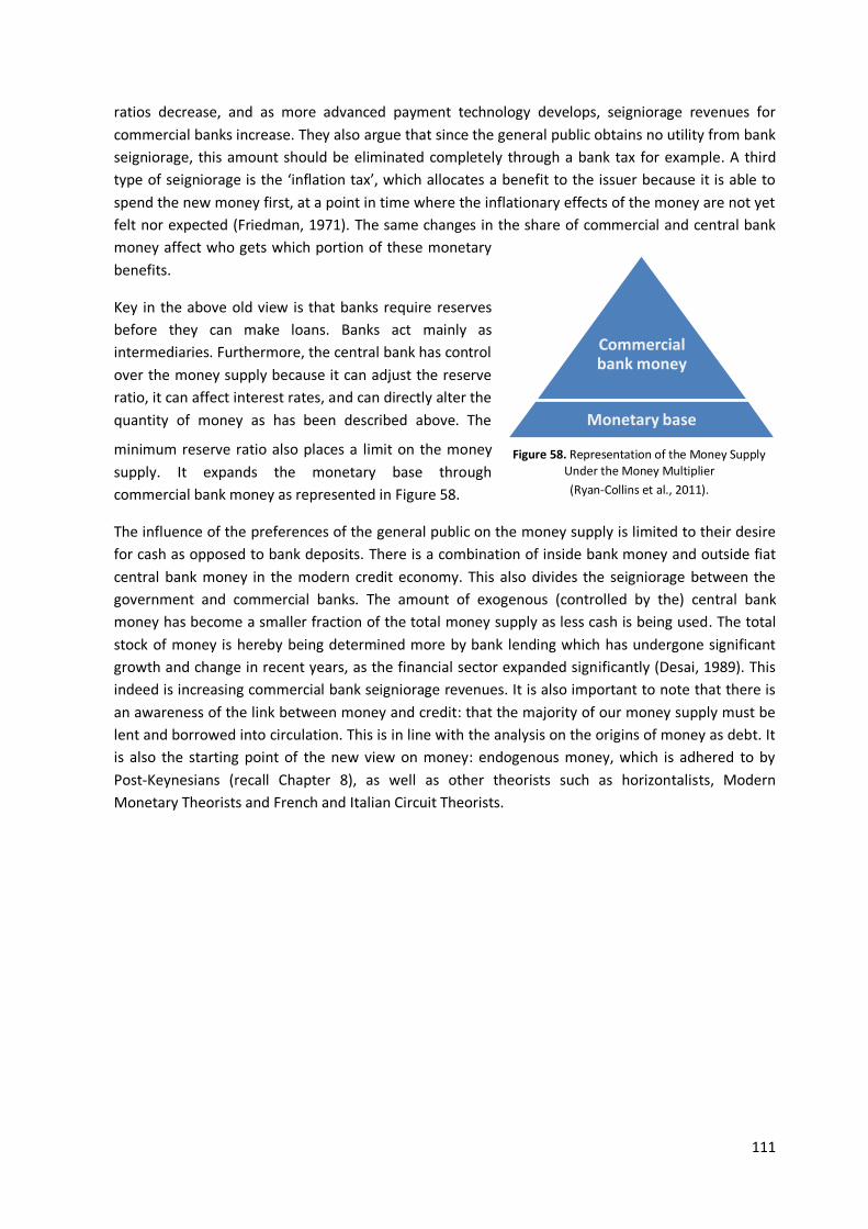
111

Commercial bank money

Monetary base

ratios decrease, and as more advanced payment technology develops, seigniorage revenues for

commercial banks increase. They also argue that since the general public obtains no utility from bank

seigniorage, this amount should be eliminated completely through a bank tax for example. A third

type of seigniorage is the ‘inflation tax’, which allocates a benefit to the issuer because it is able to

spend the new money first, at a point in time where the inflationary effects of the money are not yet

felt nor expected (Friedman, 1971). The same changes in the share of commercial and central bank

money affect who gets which portion of these monetary

benefits.

Key in the above old view is that banks require reserves

before they can make loans. Banks act mainly as

intermediaries. Furthermore, the central bank has control

over the money supply because it can adjust the reserve

ratio, it can affect interest rates, and can directly alter the

quantity of money as has been described above. The

minimum reserve ratio also places a limit on the money

supply. It expands the monetary base through

commercial bank money as represented in Figure 58.

The influence of the preferences of the general public on the money supply is limited to their desire

for cash as opposed to bank deposits. There is a combination of inside bank money and outside fiat

central bank money in the modern credit economy. This also divides the seigniorage between the

government and commercial banks. The amount of exogenous (controlled by the) central bank

money has become a smaller fraction of the total money supply as less cash is being used. The total

stock of money is hereby being determined more by bank lending which has undergone significant

growth and change in recent years, as the financial sector expanded significantly (Desai, 1989). This

indeed is increasing commercial bank seigniorage revenues. It is also important to note that there is

an awareness of the link between money and credit: that the majority of our money supply must be

lent and borrowed into circulation. This is in line with the analysis on the origins of money as debt. It

is also the starting point of the new view on money: endogenous money, which is adhered to by

Post-Keynesians (recall Chapter 8), as well as other theorists such as horizontalists, Modern

Monetary Theorists and French and Italian Circuit Theorists.

Figure 58. Representation of the Money Supply Under the Money Multiplier

(Ryan-Collins et al., 2011).

112

9.4. The new view of money: endogenous credit money.

9.4.1. The process of money creation in the new view.

Amongst others, work by Post-Keynesians (Wray, 1998; Godley, 1999; Keen, 2011), by Smithin

(2000), and Arestis and Sawyer (2006), and Ryan-Collins et al. (2011), will be used to explore the new

view. They give an extensive overview of topics such as endogenous money and credit creation,

financial instability, and the alternative monetary policy related to this new view on money.

In the new view, money is even more explicitly seen as

commercial bank debt. Money is created by the process of

credit creation by these commercial banks. While in the old

view central banks held the unique power to enable the

creation of money by increasing high-powered money, in the

new view commercial banks are able to create money largely

independent of this. The banks are still viewed as financial

intermediaries but which are able to simultaneously provide

for the conflicting demands of borrowers and lenders, because

of their administrating and negotiating expertise, because they

can pool risk, and because of government guarantees which

assure solvency and liquidity (Tobin, 1964). Simultaneous

provision signifies that a bank does not require deposits or

reserves before it makes a loan. The increase in money through

the loan occurs without any decrease of, or transfer from, someone else’s account. This is always

possible, because a loan is a mere bookkeeping entry that simultaneously creates an asset (the loan),

and a liability (the deposit) for the bank (Wray, 2002). Commercial bank money can be seen to be

able to inflate (and deflate) like a balloon around a core of central bank reserves (Figure 59) while in

the ‘old’ view it was determined by the base of the triangle (Figure 58). From this perspective, the

money supply is endogenous, determined from within the market, and not as in mainstream

theoretical models exogenously determined by the central bank.

The money supply depends on the supply of credit by commercial banks and the demand of credit

from within the economy. The reserve ratio is not there to keep a certain quantity of money in

circulation, but to ensure the payment system functions smoothly. It can always be met because a

central bank will always provide (sell) reserves to maintain its overnight interest rate target so that

the demand for reserves equals its supply (Holmes, 1969; Mosler, 1994; Wray, 2007). Note that if an

economy is on an arrangement such as a gold standard or currency board this does not apply

because then banks indeed must ensure they have enough gold or central bank reserves when they

make a loan (Fullwiler, 2009a). The old view applies in this case, because only when there is an

increase in the amount of gold in a nation or if central bank reserves increase relative to gold

reserves, can extra deposits be created. In the new view, it is the willingness of a commercial banks

to supply credit (which depends on the profitability of the loan and the credit worthiness of the

general public) and the willingness of the public to borrow, and not (excess) reserves, which

determine the money supply (Rochon, 2000).

The process of money creation is considered in more detail below. This is based primarily on work by

Ryan-Collins et al. (2011) of the New Economics Foundation, with a theoretical background of

Figure 59. Representation of the Money Supply in the New View.

(Ryan-Collins et al., 2011).

Commercial bank money

Monetary base

113

Fullwiler (2009, 2012), Wray (1998, 2011), Lavoie (2003), Arestis and Sawyer (2006), and Bezemer

(2012). Bezemer presents the fundamental principle of this analysis: double entry bookkeeping,

based on Minsky’s work on money as a balance sheet operation (Minsky, 1986). Money can be

privately created when two people enter into a forward contract with each other. The IOU or debt is

an asset for the creditor and a liability for the debtor. In other words, when someone takes out a

loan from a bank, a liability is created in the form of a debt to be paid to the bank, and an asset which

is the bank deposit, i.e. money.

In order for this process of money creation to start we first need a demand for credit. A firm or an

individual goes to a bank to take out a loan. Consider Alan who wants to borrow ₤20,000 to buy a

new car. The bank, say ABN Amro, needs to believe in the ability of Alan to pay back the loan. This

depends for example on the income of Alan, and his credit rating which is tracked by a central

authority where all loans are registered. If Alan is seen to be credit worthy, a loan contract is signed.

The principal amount, ₤20,000 needs to be paid back within a certain time, and in addition, a

percentage interest must be paid in regular installments. The loan is subsequently given within the

legal limits established by the government. It for example may have set a capital adequacy ratio,

which the bank needs to be sure it can fulfill.

From an accounting perspective, based on double entry bookkeeping, there must be an asset and a

liability created in this transaction. ABN Amro now has an asset in the form of the loan of ₤20,000,

because this is what the customer owes the bank. It also has a liability in the form of Alan’s deposit

which has been credited with ₤20,000; this is what ABN Amro owes the depositor. From the

perspective of the borrower, there is no difference in whether he lends the money from an individual

or from a bank. He still has to persuade the lender to borrow him money. However, from a system

perspective, this situation would merely be a transfer of money from the lender to the borrower. The

deposit of the lender is debited, while that of the borrower is credited. Lending from the bank,

however, creates purchasing power without reducing it for someone else, no-one else’s deposit

decreases. ABN Amro and Alan’s balance sheets (ignoring other assets and liabilities) now look like

this:

ABN Amro’s Balance Sheet

Assets What borrowers owe to the bank + bank’s money

Liabilities What the bank owes to depositors + its net worth

Loan to Alan ₤20,000 Alan’s new deposit account ₤20,000

Alan’s Balance Sheet

Assets What creditors owe the customer

Liabilities What the customer owes creditors

Alan’s new deposit account ₤20,000 Loan from ABN Amro ₤20,000

Table 8. Commercial Bank and Borrower Balance Sheet When a Loan is Given (Ryan-Collins et al., 2011; Lavoie, 2003; Fullwiler, 2012).

The loan has expanded ABN Amro’s balance sheet by adding ‘some numbers’ to it. In the words of

Schumpeter (1934): “This method of obtaining money is the creation of purchasing power by banks

… It is always a question, not of transforming purchasing power which already exists in someone’s

114

possession, but of the creation of new purchasing power out of nothing”. For a historical summary of

the view that money is ‘created out of nothing’ see King (2012). Indeed, the bank literally ‘typed

some numbers’ into Alan’s bank account. However, these numbers can be used as money. It is new

spending power: the loan creates a deposit. Note here it is important to differentiate between the

loan that exists and the deposit. It is not so that the loan is deposited. The two rather arise together,

simultaneously: the loan is the bank’s asset, and the deposit is a liability for ABN Amro. Alan can use

his deposit to pay for the car, which debits his account, and credits that of the car dealer, Bill. Bill can

subsequently use his deposit, to pay for his groceries, the school fees of his children, etc. While the

bank’s debt (the deposit) is circulating as money, the original loan continues to exist. Alan’s debt still

has to be repaid with interest and on due dates.

Let us now consider the simplest situation in which Alan’s deposit is purely used to save a part of his

salary, pay interest on the loan, and pay back the loan in one time, and no other transactions.

Depending on his income, the deposit will build up over time back to the original level of the loan. At

this point the loan can be paid back to the bank. When this is done, money is extracted from the

economy – it is literally annihilated and the money stock decreases. The asset and liability are both

removed from ABN Amro’s balance since the loan to Alan (asset for the bank) is paid back, and the

deposit that was created for Alan (liability for the bank) is spent on paying back the loan. Note that it

is not the original deposit that is ‘paid back’; the deposit is a mere account of the total number of

Pounds that Alan has. The deposit was debited when Alan paid for the car, and credited over time as

his salary was paid (debiting the account of his employer). One can follow the transactions in the

system, and denote these in Pounds, but one cannot follow the deposit made by the bank. These

simply exist, and record the transactions. For a single bank it is easy to settle these transactions as it

can credit and debit its account holders very easily; it is a question of ‘keeping score’. However,

between banks this becomes more complicated, a transaction settlement mechanism is needed,

which is described next.

The payment from Alan to his car dealer Bill is likely done by electronic transfer. If Bill and Alan have

the same bank, this is a simple accounting entry for ABN Amro where the ₤20,000 is removed Alan’s

account, and added to Bill’s account. The deposit, remains a liability for ABN Amro. The reduction in

this liability in the form of Alan’s new deposit account is simply compensated for by an increased

liability in the form of the new deposit in Bill’s account. The balance remains. However, Bill may not

have the same bank as Alan. Say Bill banks with Barclay’s Bank. One can imagine that ABN Amro

needs a way to ‘convince’ Barclay’s to hold the liability to Bill (Bill’s deposit). There are two ways in

which the banks can settle the transaction.

First, the banks may have accounts with each other, enabling such changes to occur more easily –

bilateral settlement. ABN Amro has an account at Barclay’s from which it can say to deduct the

₤20,000 that is transferred from John to Bill’s account. This reduces Barclay’s debt to ABN Amro, and

Barclay’s takes on the debt (liability) to Bill. If ABN Amro does not have any money in its account at

Barclay’s, Barclay’s could also give ABN Amro a loan. By keeping track of the transfers between each

other, settlement is made easier since a large portion of transfers cancel each other out every day.

This process is referred to as intra-day intra-bank clearing. For example, there may be other

individuals that are transferring money between the banks, and only the net change has to be

transacted at the end of the day. In this way, the liability to Alan of ABN Amro, because he had a

deposit there, becomes a liability of Barclay’s to Bill.

115

Second, the transaction could be settled by the banks by moving their reserves at the central bank.

All commercial banks hold reserves at their central bank in order to enable such transactions. Simply

put, individuals have bank accounts with commercial banks to make payments and commercial banks

have accounts with the central bank to make some of their payments. Note that this is less needed if

the interbank lending market is strong – banks trust each other and overnight loans, with interest,

can be rolled over – as this enables commercial banks to settle transactions amongst themselves. If

this is not so, banks will make more use of central bank reserves to settle transactions.

In the example, ABN Amro would need to transfer ₤20,000 in reserves to Barclay’s central bank

reserve account. ABN Amro debits its reserve account by ₤20,000 of central bank reserves, which

credits Barclay’s reserve account by ₤20,000 of central bank reserves. Again, Barclay’s is

‘compensated’ for the additional liability (Bill’s deposit) it has to take on. Assuming that ABN Amro

had no reserves to start with, the liability for ABN Amro that stands opposite its asset (the loan to

Alan) in its books is now in the form of a loan in the form of reserves.

ABN Amro’s Balance Sheet Alan’s Balance Sheet

Assets Liabilities Assets Liabilities

+ Loan to Alan + Deposit of Alan + Deposit at ABN + Loan from ABN

- Reserves - Deposit by Alan - Deposit at ABN

+ Reserves + Borrowings + Car

Barclay’s Balance Sheet Bill’s Balance Sheet

Assets Liabilities Assets Liabilities

+ Reserves + Deposit by Bill + Deposit at Barclay’s

- Car

Table 9. Balance Sheets When Alan Pays Bill and Banks Settle With Reserves (Fullwiler, 2012).

In the balance sheet above, the process occurs in three steps. First (yellow), the loan and deposit are

created simultaneously. Secondly (green), the transfer of the car occurs which reduces both the

reserves of, and deposit at, ABN Amro, and increases the deposit and reserves at Barclay’s. Alan’s

deposit is reduced and transferred to Bill’s at Barclay’s, and the car changes hands. Thirdly (blue), if

ABN Amro has no reserves and thus utilized the central bank’s overdraft facility to transfer reserves

to Barclay’s, it has to settle this, by borrowing central bank reserves. Note that if ABN Amro had

enough reserves to make the transaction to Barclay´s, this third step would not be needed.

The central bank reserve accounts hereby enable settlement between different banks – they ensure

the payment system functions, and convince bank customers that other liquid assets, such as cash,

are readily available should they demand them. The bank does not necessarily require reserves

before it makes a loan. Note that ABN Amro still has a net balance with positive reserves on the

assets side, and positive borrowings on the liabilities side. ABN Amro can have loaned the central

bank reserves from another bank in the Interbank money market (if one bank is ‘long’ on reserves –

has excess, and another is ‘short’ – has too few), or can have borrowed them from the central bank

in the form of an overdraft. This must be cleared at the end of the day by nonetheless borrowing

116

from other banks, or with an overnight loan from the central bank, e.g. backed up by certain

collateral (Fullwiler, 2012).

Historically, the origins of reserves lie in the deposits that commercial banks had with each other in

order to ease payments and hereby increase the liquidity of the banking system (Feinman, 1993).

Over time, these reserves were made compulsory, and established at the central bank – the legally

required reserve ratio as we know it today. The fact that the required reserve requirement does not

play a role in determining bank lending or the money supply is revealed by the requirements of

nations. Not all nations have a mandatory reserve ratio (

Table 10), relying on the commercial banks to estimate their need for reserves to ensure there is

enough liquidity.

Countries No RR 0-5% 6-15% >16%

High income 25.9 55.6 14.8 3.7

Medium income 2.8 34.7 47.2 15.3

Low income 0.0 27.3 59.1 13.6

Table 10. Reserve Requirements (RR) of Countries by Income Level in 2010 (Gray, 2011).

Especially in high income countries, there is no required reserve ratio, stemming from decades of

deregulation and a reliance on higher levels of interbank trust and lending as well as voluntary

reserves. Medium and low income countries are characterized by higher reserve requirements, on

average between 6% and 15%, to guarantee liquidity and solvency of banks as well as enable greater

monetary control (Gray, 2011).

Interest is paid on any borrowed reserves, and the interest rate in the Interbank money market (e.g.

Libor, Euribor) is closely related to that which the central bank sets on borrowed reserves. In order to

maintain its interest rate target, the central bank will always increase its supply of reserves whenever

there is an increase in demand. Furthermore, the fact that reserves are automatically created by the

central bank in the form of the overdraft facility ensures that these will always be there, in order to

guarantee liquidity. In times of economic prosperity where banks create significant amounts of credit

(i.e. money), there will be more pressure on the central bank to increase reserves to make sure that

the payment system continues to work. The alternatives would be to refuse to issue new reserves

which would lead to a credit crunch, or to relax the reserve ratio which is a rather blunt tool.

Therefore, the central bank’s policy choice will likely be to create new reserves (base money) if there

is a demand for them. This guidance by the market in the money supply has been referred to as an

endogenous money supply. In terms of the money creation process, the reserves are thus irrelevant

as they are there merely to limit fluctuations in the interest rate and ensure the payment system

works so that transactions occur smoothly. They are not there to affect or limit the quantity of

money:

“Monetary policy sets the price of money, which only indirectly determines the quantity. It will be

shown that the overnight rate of interest is the primary tool of monetary policy…. The money

multiplier is backwards. Changes in the money supply cause changes in bank reserves and the

monetary base, not vice versa.

(Mosler, 1994).

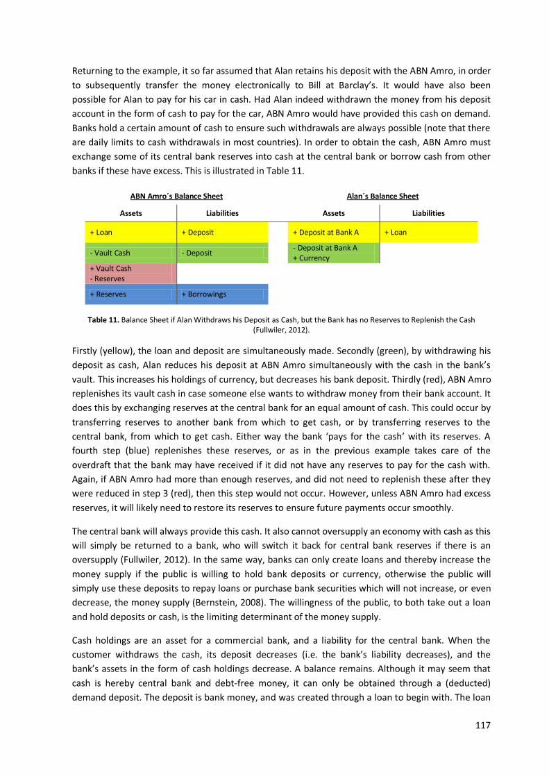
117

Returning to the example, it so far assumed that Alan retains his deposit with the ABN Amro, in order

to subsequently transfer the money electronically to Bill at Barclay’s. It would have also been

possible for Alan to pay for his car in cash. Had Alan indeed withdrawn the money from his deposit

account in the form of cash to pay for the car, ABN Amro would have provided this cash on demand.

Banks hold a certain amount of cash to ensure such withdrawals are always possible (note that there

are daily limits to cash withdrawals in most countries). In order to obtain the cash, ABN Amro must

exchange some of its central bank reserves into cash at the central bank or borrow cash from other

banks if these have excess. This is illustrated in Table 11.

ABN Amro´s Balance Sheet Alan´s Balance Sheet

Assets Liabilities Assets Liabilities

+ Loan + Deposit + Deposit at Bank A + Loan

- Vault Cash - Deposit - Deposit at Bank A + Currency

+ Vault Cash - Reserves

+ Reserves + Borrowings

Table 11. Balance Sheet if Alan Withdraws his Deposit as Cash, but the Bank has no Reserves to Replenish the Cash

(Fullwiler, 2012).

Firstly (yellow), the loan and deposit are simultaneously made. Secondly (green), by withdrawing his

deposit as cash, Alan reduces his deposit at ABN Amro simultaneously with the cash in the bank’s

vault. This increases his holdings of currency, but decreases his bank deposit. Thirdly (red), ABN Amro

replenishes its vault cash in case someone else wants to withdraw money from their bank account. It

does this by exchanging reserves at the central bank for an equal amount of cash. This could occur by

transferring reserves to another bank from which to get cash, or by transferring reserves to the

central bank, from which to get cash. Either way the bank ‘pays for the cash’ with its reserves. A

fourth step (blue) replenishes these reserves, or as in the previous example takes care of the

overdraft that the bank may have received if it did not have any reserves to pay for the cash with.

Again, if ABN Amro had more than enough reserves, and did not need to replenish these after they

were reduced in step 3 (red), then this step would not occur. However, unless ABN Amro had excess

reserves, it will likely need to restore its reserves to ensure future payments occur smoothly.

The central bank will always provide this cash. It also cannot oversupply an economy with cash as this

will simply be returned to a bank, who will switch it back for central bank reserves if there is an

oversupply (Fullwiler, 2012). In the same way, banks can only create loans and thereby increase the

money supply if the public is willing to hold bank deposits or currency, otherwise the public will

simply use these deposits to repay loans or purchase bank securities which will not increase, or even

decrease, the money supply (Bernstein, 2008). The willingness of the public, to both take out a loan

and hold deposits or cash, is the limiting determinant of the money supply.

Cash holdings are an asset for a commercial bank, and a liability for the central bank. When the

customer withdraws the cash, its deposit decreases (i.e. the bank’s liability decreases), and the

bank’s assets in the form of cash holdings decrease. A balance remains. Although it may seem that

cash is hereby central bank and debt-free money, it can only be obtained through a (deducted)

demand deposit. The deposit is bank money, and was created through a loan to begin with. The loan

118

that originated the money, still exists and still needs to be paid back. In essence, the use of cash

instead of the demand deposit is a mere swap of form from a promise to pay by the commercial bank

to a promise to pay by the central bank. Both forms of money have no backing, they are forms of fiat

money. As are central bank reserves. If you would take up these promises to pay, the central bank

and the commercial bank would both give you the same amount in either cash, bank or central bank

(if you are a commercial bank) deposits, in return. In addition, State guarantees of commercial banks

and their deposits further reduce the difference between commercial bank and central bank money.

Given these overviews, the table below provides the main differences between the ‘new’ and ‘old’

view on money.

Subject The ‘Old’ View: Exogenous Money The ‘New’ View: Endogenous Money

Base money (reserves) vs. higher monetary aggregates

Reserves move first, then broader aggregates due they are ‘lent out’. Deposits precede loans.

Changes in reserves follow changes in higher monetary aggregates. Deposits and loans are created simultaneously.

Role of the central bank The central bank can, as they desire, control the quantity of base money. The multiplier matters – there is a stable money demand function.

The central bank must passively accommodate the banking system to avoid economic problems. The multiplier is irrelevant.

Link between reserves and bank lending

Bank lending depends on their reserves.

A bank decides whether to lend irrespective of its reserves, reserve decisions are taken after lending.

Effect of changes in the monetary base

An increase in the money base (reserves), impacts bank lending and other economic indicators.

Increases in the money base are rare and mainly to ‘oil’ the (payments) system between banks.

Role of debt in the economy The distribution, not the level of private debt matters in the economy.

The level of private debt affects the economy.

Table 12.The ‘Old’ vs. ‘New’ View on Money.

The main difference between the theories lies mainly in the causality between bank lending and

reserves. The old view finds that credit money expansion follows the expansion of base money /

reserves: banks acquire reserves and then lend. The new view on the other hand claims commercial

banks first make loans, and then afterwards consider the reserves they need / require.

This may seem like an irrelevant difference but it has a number of main implications. First, before

lending, a bank has adequate reserves, then any bad loans will only create a problem for the

respective bank. However, in the new view, banks are highly dependent on each other for reserves,

in which case a bad loan can cause instabilities in the entire banking system. Second, since money is

created by commercial banks through bank loans (double-entry bookkeeping), debts do not cancel

out in the aggregate and the economy can be over-indebted. By expanding the money supply, the

stock of debt is also expanded. This debt (credit) needs to go to productive investments to generate

additional future income to be able to service the added debt. If it rather bids up the price of assets

(inflation), there is no extra income generated to service the higher debt level. The inability to service

the debts has a negative effect on the economy. Money, because it is created as interest-bearing

commercial bank debt, matters, and does not play a neutral role in the economy in the long-run.

However, there exists also considerable overlap in the theories. There are both exogenous and

endogenous elements in both theories. The old view namely acknowledges that given an

exogenously set amount of reserves, the amount that commercial banks lend out, is largely

119

endogenously determined depending on the supply and demand for credit in the market. The new

view claims the latter are the only drivers of bank lending and that reserves do not matter; however,

they do acknowledge that the interest rate as set by monetary authorities is an exogenous constraint

to bank lending. The next section focuses on the endogenous component of the money creation

process: how the money supply thus rather depends on the portfolio choices of the public (firms and

households), and the willingness of commercial banks to provide it (profitability analysis), all within

the legal framework of government.

9.4.2. The business model of a commercial bank in the new view on money creation.

According to Cavelaars and Passenier (2012), commercial banks have three main sources of income:

interest income, fee income, and trading income. Our analysis focuses on the first source, which

stems from its credit creation activities. Interest income in turn also derives from three main sources.

First, it is “information-based monopoly rent” (Cavelaars and Passenier, 2012) earned on general

lending. Second and more specifically, the bank earns on transforming maturities by borrowing short

and subsequently lending long. The resulting spread is on average positive, but also increases the

bank’s vulnerability to bank runs. Third, banks will demand a premium to compensate for the risks it

takes in lending.

Purely focusing on this source of income, a commercial bank’s business model entails constantly

trying to increase earnings on assets, minimize payments on liabilities, and minimize capital held

since equity is more costly than debt2 (Fullwiler, 2012). This implies that banks aim to expand their

asset side through making (credit worthy) loans, and attract as many deposits as possible since these

are the cheapest liability. It is in the interest of a commercial bank to obtain deposits because in a

larger bank, transactions are more likely to occur between its own clients which does not require

(costly) commercial bank reserves to settle the transaction. These reserves are interest-bearing

(recall they must be borrowed from the central bank or other banks) and so this is an advantage for a

large bank. It can go on to hold more profitable assets. Without deposits, a bank can make a loan,

but if the simultaneously created deposit is moved to another bank, this credit creation is less

profitable than were it to remain in the same bank. The bank could raise the interest rate on

borrowing to deal with this, but in a competitive market this will result in the borrower taking the

loan out from another bank.

There are a number of general factors that influence bank income and the profitability of loans.

These are as follows. In general, bank income will likely be higher if the rate of money creation is

higher (this does depend on a bank’s capital constraints which is considered later). Banks are

assumed to profit from lending, and a higher rate of money creation is an indication of increased

credit creation. Figure 60 shows that the growth rate of the broad money supply has been increasing

over time, until the crisis.

2 Debt is ‘senior’ to equity – debtors are paid before equity holders in the case of bankruptcy thus equity

holders require a risk premium, and there may be tax advantages to debt.

120

Figure 60. Growth Rate of M4 in the UK (Bank of England, 2012b).

Note that this is the growth rate of M4, so the trend is even an acceleration of money creation until

2007. At this point the ‘credit crunch’ by which the recent financial-economic crisis was characterized

is clearly seen. The growth rate dropped from about 9% to 2% but remained positive. The increase in

debt repayment that complemented this will have likely put a downward pressure on bank income.

A lower (required) capital ratio, or higher leverage, will increase the returns for a bank. Figure 61

shows the rising trend in leverage of UK banks since the 1970s. Leverage here is defined by the ratio

of the bank’s total assets to shareholder claims (equity or net worth).

Figure 61. UK Bank Leverage from 1960-2010 (Bank of England, 2010).

Following a period of deleveraging in the early 1960s there has been a general increase in leverage. It

is only with the recent crisis that bank’s have started to retain more equity (capital) and reducing

leverage again. Profitability is further positively related to the interest rate spread that a bank earns

on its loans and deposits and negatively related to the share of cash used in the economy. Figure 62

reveals the reduction in the share of notes and coins in M1 and M4 in the UK.

0

2

4

6

8

10

12

30-s

ep-9

8

30-s

ep-9

9

30-s

ep-0

0

30-s

ep-0

1

30-s

ep-0

2

30-s

ep-0

3

30-s

ep-0

4

30-s

ep-0

5

30-s

ep-0

6

30-s

ep-0

7

30-s

ep-0

8

30-s

ep-0

9

30-s

ep-1

0

30-s

ep-1

1 Gro

wth

rate

(%

), s

eas

on

ally

ad

just

ed

121

Figure 62. Share of Notes and Coins in Broad Money Supply M1 and M4 in the UK (Bank of England, 2012).

In the 1980s the share of cash (notes and coins) in the broad money supply decreased from about 9%

to 4%, where it has been stable since. A similar trend is reflected in M1 where notes and coin

reduced in share from about 14% to just 4%. This indicates the diminishing share has not just been

due to the development of higher monies but rather increased use of deposits and bank cards. As

electronic banking and payment becomes more popular, this share may decrease further. This

decreases the need for banks to hold cash, which is costly not only for safety reasons but also

because it has to be borrowed from the central bank. Its own accounts, bank money, do not. A

number of other factors influence the need to hold (costly) reserves which are described below.

If the rate of circulation of unlent reserves is higher bank income will benefit through the same

channel, and if more transactions occur within the same bank, fewer reserves need to be held. A

bank thus benefits from a more concentrated financial sector not only because of the benefits of

greater market power and less competition. It also benefits because this reduces the number of

transactions that its clients will undertake with a different bank, which it needs to settle with (costly)

reserves or interbank loans. This is a self-enhancing cycle, as higher profits from greater market share

enable a bank to expand its market share further through for example an acquisition. In Part I we saw

that in the UK there was increased concentration in the banking sector yielding that the top 3 banks

now own more than 50% of the banking sector’s total assets (Haldane et al., 2010). Interbank trust

also plays an important role in this, as it also enables banks to settle transactions on their own

accounts without central bank reserves. Figure 63 provides an indication of interbank lending in the

UK.

0

0.01

0.02

0.03

0.04

0.05

0.06

0.07

0

0.02

0.04

0.06

0.08

0.1

0.12

0.14

0.16

30

-sep

-86

31

Mar

88

30

-sep

-89

31

Mar

91

30

-sep

-92

31

Mar

94

30

-sep

-95

31

Mar

97

30

-sep

-98

31

Mar

00

30

-sep

-01

31

Mar

03

30

-sep

-04

31

Mar

06

30

-sep

-07

31

Mar

09

30

-sep

-10

31

Mar

12

Shar

e in

M4

Shar

e in

M1

Notes and coin in M1

Notes and coin in M4

122

Figure 63. Interbank Lending in the UK Monetary Financial Institutions' Net Lending to Other Financial Corporations (Bank of England, 2012).

Between 1997 and 2008, interbank lending increased four-fold. The crisis has abruptly cut interbank

trust and lending, as seen in the reduction in interbank loans since 2008.

The aforementioned factors impact bank income and the profitability of bank lending. However,

there are some limitations to the activities of banks. The general mechanism is depicted in a

conceptual model in Figure 64. Continuous arrows represent the main determinants or actions, while

dotted arrows are secondary (re)actions that banks (can) influence. The description following the

figures relates back to the various numbered errors.

Figure 64. Determinants of the Money Supply.

In the system there exists a central bank that has a certain amount of base money or reserves (1).

These are in essence outside of the money system, they do not have an effect and cannot result in

inflationary pressures for example, until they are loaned into the economy via commercial banks.

They are however necessary to ensure ease of payment settlements for commercial banks. The

demand for the reserves comes from commercial banks (2), and in order to maintain an interest rate

target and ensure stability in the system the central bank will respond by providing these reserves

(3). In principle, it could also refuse to do so and let the interest rate rise, reducing credit creation.

0

200000

400000

600000

800000

1000000

1200000

30-s

ep-9

7

30-n

ov-

98

31-j

an-0

0

31 M

ar 0

1

31 M

ay 0

2

31-j

ul-

03

30-s

ep-0

4

30-n

ov-

05

31-j

an-0

7

31 M

ar 0

8

31 M

ay 0

9

31-j

ul-

10

30-s

ep-1

1 St

erl

ing

mill

ion

s (s

eas

on

ally

ad

just

ed

)

1 2

3

4

5

6 7

8

9 10

123

The money supply in circulation is determined by the willingness of the public to borrow, and of

commercial banks to lend at given interest rates. Consumer demand (5) can be enhanced, during

asset bubbles (6). For example, in a housing bubble, individuals may be encouraged to borrow to buy

a house in the expectation that they can pay back the loan, with interest and profit, because of rising

prices. The house provides the collateral necessary for the bank to make a safe loan, and thus there

is enough incentive for both parties to undertake the transaction. In general, in time of economic

optimism, a boom, consumer demand for credit increases in anticipation of higher income, and it

decreases if there is a recession.

The willingness of commercial banks to lend, depends on the profitability analyses of these banks as

they operate to maximize their profits (4). This profitability depends on their ability to maintain their

capital adequacy requirements (7) as it expands its balance sheet by creating new loans / deposits

and on the ease for banks to obtain (cheap) deposits after a loan is made (Fullwiler, 2012). This is a

different restriction than any reserve requirement, which does not limit bank lending as explained

above (it rather enables the payment system). The capital adequacy requirements entail that banks

are by regulation often required to hold a certain portion of their assets in the form of capital, where

capital is the net worth, or equity of the bank. In most countries these are set in the Basel Accords

(see BIS, 2012 for more details). The latest Basel (III) capital requirements differentiate assets

according to their risk profile, and defines two different forms of capital (Tier I and II). These

regulations attempt to reduce the risk of bank default and ensure banks can honor withdrawals.

However, the effect of capital requirements have changed significantly with the financial innovation

of the past decades (8). Deregulation has further enabled this, for example, allowing banks to move

various liabilities off of its balance. These off-balance sheet assets and liabilities are not weighted in

risk evaluations. Furthermore, during a boom, lower risk estimates of assets and collateral enables

banks to hold less capital, as do higher lending and greater (interest) profits in such a period. In

general, the loans banks create generate interest earnings, which can easily be retained to maintain

capital levels. In this sense, increasing loans generates its own increase in potential capital for banks.

The willingness of commercial banks to provide credit, also depends on the credit worthiness, or the

ability to repay, of the borrower (9). The development of banks becoming ‘too big to fail’ has

provided banks with certainty (10) because States have responded with providing guarantees and

bail-outs. Government policies to for example enhance home ownership may also reduce the

limitation of this channel as banks are stimulated to provide loans to less credit worthy individuals.

Furthermore, changes in the banks’ original business model from ‘originate to hold’ to ‘originate to

sell’ has reduced the importance of the credit worthiness of borrowers. Nevertheless, it is not so that

banks will lend (create) infinite amounts of money. An individual bank, needs to maintain its credit

worthiness in order to be competitive in the market, giving them a constant incentive to reduce

(visible) risk while extending as much credit as possible. Furthermore, depending on a variety of

other factors such as market interest rates, increasing the quantity of loans may not be the most

profitable strategy for a bank.

Although banks can create money, they cannot do so to finance their own expenditures as the

creation of money – a deposit (a liability for the bank) requires also an entry on the asset side of the

balance sheet (e.g. a loan) by the rules of double-entry bookkeeping. They do make a profit via the

interest that is charged on the loans that they create. The standard definition of seigniorage, the

difference between the productions costs of money and its face value for which it is sold, however,

124

does not apply to commercial bank created money. This is because the loans they create will at some

point be paid back (although this can take decades as they are largely rolled over). The banking

system also does not capture direct seigniorage benefits of money creation ‘out of nothing’ (occurs

electronically at negligible cost), because for every loan a bank extends, they also create a deposit,

upon which the system as a whole pays (some) interest. There is however a clear benefit when

comparing to a system in which a bank would act as a mere intermediary. If the central bank would

for example create and spend money into the economy, not all money created would be associated

with a (for the banks) profitable loan. A loan from the central bank or government (read general

public) would be money’s counterpart, instead of a bank loan. Only a part of the money supply could

subsequently be saved and loaned by private parties. Assuming more loans results in higher profits

for the banks, this results in extra income compared to the alternative system. It is not possible to

place an exact monetary value on this benefit in the current situation because the alternative system

does not exist. Furthermore this is not seigniorage in the sense that the bank actually receives this

income.

Without having to pay the central bank for the money it loans out, total profits equal the interest

rate spread between what the bank charges on the loan and pays on the associated deposit. Let us

say 5%-3% = 2%. However, if there is new money that enters the economy through for example

government spending, then when it is deposited the bank has to pay 3% interest on it without there

being a complementary loan from which it benefits. The difference between earning 2% and having

to pay 3% on all additionally created money is 5%, the interest rate charged on loans. This is how the

banking system benefits, but it does not receive this in payment. Alternatively, a commercial bank

would have to borrow the extra money they create from the central bank, and pay the central bank a

particular base rate for it, let’s say 1%. In this case, profits of expanding the money supply equal the

interest rate spread on loans and the associated deposit 5%-3%=2%, minus the 1% that it has to pay

the central bank to get this additional money. Total profits reduce to 1%. In this case, the additional

seigniorage profits that a bank has because it can create money equal the interest rate spread minus

the central bank base rate. Robertson and Huber (2000) find this advantage to have a value of about

₤21 billion per year for commercial banks in the UK. The latter case is somewhat similar to the

current situation if banks have to provide cash, because they have to borrow this at interest from the

central bank, reducing profits. They also pay the central bank interest for any loaned reserves. The

increase in the proportion of electronic bank money compared to cash, and decreased need of

central bank reserves, has therefore reduced the costs for banks and increased their profits,

decreasing those of the central bank and subsequently government.

The current system not only gives commercial banks additional real income as compared to a

situation of them being an intermediary, but, it also widens the scope of short-termism in

investments to all money in the economy. It namely requires interest to be paid to commercial banks

over the entire money supply. Interest encourages short-termism because it makes long-term

investments relatively more expensive than shorter ones. For example, at a 5% interest rate, a

planted oak tree that provides ₤1000 in 100 years and a pine tree that provides ₤100 in ten years are

worth ₤61 and ₤7.60 respectively today (Lietaer et al., 2012). Clearly, the former short-term

investment will be made. For a demurrage currency with a negative interest rate, the opposite is

true: long-term investments are favored.

125

Furthermore, the system also benefits those first beneficiaries of the expanded money supply: credit-

worthy individuals or firms with high private return investments. These members of the public do not

bear the inflationary effects of the monetary expansion as being closest to the point of money

creation. The need for a project with high private and marketable returns to obtain a loan will also

make those human and natural resources that are unprotected because their costs are difficult to

internalize (e.g. the atmosphere, child labor) become exploited as they provide a high return. This

misallocation of resources is rational and optimal from an individual perspective (of the bank and the

debtor), but from a long-term social perspective it may have suboptimal results.

One may ask how bank money in this form has become so generally accepted. Bank money has

become popular due to its ease and safety for consumers and producers, encouraged by marketing

campaigns to pin or chip instead of pay with cash. However, it is only utilized and trusted because

the central bank ensures direct convertibility of demand deposits (bank money) for cash and because

taxes can be paid with this bank money. This aligns with the perspective in Chapter 7 that money is a

creature of the State (Knapp, 1905). Applied to the creation of money, this implies that the State first

has to create money, and then implements a tax in order to create a demand for this money:

“logically, and in practice, government spending comes prior to taxation” (Tcherneva, 2006) and “the

fact that taxes need to be paid gives value to the money of the economy” (Minsky, 1986). It is not the

government that needs to tax its population to obtain their money, but the population needs the

government’s money to pay taxes (Wray, 1998). A government with a sovereign currency can always

expand its fiscal position to finance its expenditures (Fullwiler, 2009b). However, today, it is not the

government that creates the money supply, but for the largest part commercial banks and the

government accepts this bank money as payment for taxes. It is the direct convertibility between

government or central bank money and commercial bank money that has made bank money a

perfect substitute. The demand for bank money is derived from the ability to pay the State in it.

However, the problem remains that private banks can go bankrupt.

In addition to accepting commercial bank money for tax payments, national governments have also

in many countries limited themselves to utilizing existing money to finance expenditures instead of

creating it themselves or by lending from the central bank (e.g. Article 123 of the EU Lisbon Treaty).

Bezemer and Gardiner (2010) explain how these restrictions on central bank lending to government

restrict monetary policy influences on liquidity. In double entry bookkeeping, for every liability there

must be an asset of equal magnitude. If a government could lend from a central bank, this would

create assets with the central bank, which could be complemented by commercial bank liabilities.

This would enable both monetary expansion or contraction as well as more influence on bank

behavior by in this manner affecting their liquidity. The numerous other possibilities that could open

up if money, fiscal policy, and monetary policy are interpreted differently are explored by Mosler

(2010). It places public deficits and other debts in an entirely different perspective, bringing the

analysis of money back to the real economy. However, there is clearly a reason behind the

restrictions on government lending and money creation. They have been in response to experiences

of excessive government money creation and spending, of which inefficient investments and (hyper)

inflation were the result (Zarlenga, 2002). However, Zarlenga also describes that these fears and

charges have been largely misplaced. It has nonetheless tilted the balance away from public

intervention in money creation, and as seen so far in this chapter, towards private control over the

money supply. The 2007 crisis may well have illustrated that a more balanced approach is required.

126

9.4.3. Evidence for the new view on money creation.

Although there is as of yet no mainstream macro-economic textbook based on this perspective (see

for a first attempt Godley and Lavoie, 2007), there is clear econometric and empirical evidence for

the endogenous money view, even from research by neo-classical economists. Fama and French

(1999) for example find that “the source of financing most correlated with investment is long-term

debt” for American publically traded non-financial firms between 1951 and 1996 (Figure 65).

Figure 65. Corporate investment financing (Fama and French, 1999).

The correlation between firm investment and new stock issues (equity) is just 0.19, 0.56 with

retained cash earnings (RCE), and a significant 0.79 with long-term corporate debt. There is further

evidence that debt, as represented by broad credit created by banks lead the money supply (Kydland

and Prescott, 1990), which would not be expected if savings are first needed to fund investment,

lending, depositing and relending takes time, and if reserves limited bank lending. In this case one

would rather expect there to be a time lag between the monetary base and other higher aggregates.

“There is no evidence that either the monetary base of M1 leads the cycle, although some economists

still believe this monetary myth. Both the monetary base and M1 series are generally procyclical and,

if anything, the monetary base lags the cycle slightly … The difference in the behavior of M1 and M2

suggests that the difference of these aggregates (M2 minus M1) should be considered … The

difference of M2 – M1 leads the cycle by even more than M2, with the lead being about three

quarters”.

Kydland and Prescott (1990).

127

Caporale and Howells (2001) base a causality test on UK data to determine whether loans create

deposits. The traditional bank’s balance sheet (Flow of Funds identity) and ‘credit counterparts’

approach have both always stated that changes in bank loans (to the non-bank public and

government) must equal changes in deposits and notes and coins held by the public (the money

stock). However, the authors argue that while this identity must always balance, it can be rewritten

such that the a change in base money appears on the right-hand side implying the money stock is

exogenously determined by changes in central bank reserves. Using a Vector Autoregression (VAR)

and not a bivariate causality test to determine the direction, the authors control for any omitted

third factors, such as GDP that drive the demand for loans. As explained above, when a bank creates

a loan (an asset for the bank), it simultaneously creates a deposit, a liability for the bank but an asset

for an individual to use in the real economy. In this sense, a loan creates a deposit. This deposit is

likely to immediately be spent on what the loan was taken out for, increasing deposits for other

people in the process. Caporale and Howells (2001) find that loans create deposits.

The money multiplier model of banking would further predict that there is more money in the

economy than debt because for a stock of money a certain percentage cannot be loaned out. The

difference would equal the base money in the economy. However, in practice we see quite the

opposite, debt levels in the UK as well as the US exceed monetary aggregates (Keen, 2009b). In the

same way, the UK has seen an immense increase in higher monetary aggregates without an increase

in the base money (M0) that would be expected under the money multiplier model given a stable

money multiplier (Figure 66). Although one can expect the multiplier to have altered somewhat given

decreases in the currency holdings ratio (public cash demand) and the reserve ratio (see section 9.3),

this cannot account for the discrepancy seen in the figure below.

Figure 66. Negligible Increase in M0 Despite Rapidly Rising M1-M4 in the UK (Bank of England, 2012a).

Arestis and Sawyer (2008) also consider the endogenous creation of credit money with commercial

banks, to which they refer as the ‘New Consensus in Macroeconomics.’ After presenting the main

0

500000

1000000

1500000

2000000

2500000

3000000

sep

-97

apr-

98

no

v-98

jun

-99

jan

-00

aug-

00

mar

-01

oct

-01

may

-02

dec

-02

jul-

03

feb

-04

sep

-04

apr-

05

no

v-05

jun

-06

jan

-07

aug-

07

mar

-08

oct

-08

may

-09

dec

-09

jul-

10

feb

-11

sep

-11

apr-

12

Mo

nth

ly a

mo

un

ts o

uts

tan

din

g

(ste

rlin

g m

illio

ns

seas

on

ally

ad

just

ed)

M0

M1

M2

M3

M4

128

mechanisms of this theory, they link it to monetary policy, revealing that this explanation of money

corresponds better with the effects of monetary policy in reality. In Galbraith (1975), the failed

monetary policy of the United States in the 1930s reveals the lack of power of the Federal Reserve in

affecting the money supply confirming that “it was the state of trade that ruled” (Galbraith, 1975)

the money supply – i.e. the market. At the same time, government borrowing and spending through

public works directly created and injected money into the economy with a real effect.

Keen (2009a, 2012a) explains along similar reasoning why the recent bailouts of the financial sector

were not able to prevent a recession. These were based on the assumption of a money multiplier

which did not exist (Keen, 2000; Carpenter and Demiralp, 2012). Increasing the money supply by

increasing the commercial banks’ central bank reserves does not increase lending and money from

the endogenous perspective, since these are dependent on the trust and demands of the non-bank

sector which remained low as their level of debt had become too high. Galbraith already stated this

in 1975:

“The largest part of the supply of money, as by now will be adequately understood, is deposits in

banks. These come into existence as people and firms borrow money. If business is sufficiently bad,

profit prospects sufficiently dim, gloom sufficiently deep, businessmen may not borrow money. Then

no deposits are created, no money comes into existence. The banks can be provided with cash for

reserves by purchases of government securities by the Federal Reserve Bank from the banks or their

customers. This cash will then lie fallow in the banks.”

(Galbraith, 1975).

This reasoning has been applied by Koo (2008) to Japan’s deflationary experience, which started in

the 1990s following the collapse of a real estate and stock market bubble. He argues that in the

‘balance sheet recession’ that occurred, the money supply in Japan did not respond to monetary

policy because the private sector was in a process of deleveraging. Despite quantitative easing and

even negative real interest rates, firms and households could not be induced to take on more debt,

limiting any increase in the money supply.

For the same reason, the massive increase in central bank reserves (base money) that has occurred in

the recent Western crisis has not created the inflation that would be expected with the money

multiplier model. In the US for example, base money doubled in four months from October 2008 to

February 2009 (it also doubled between 1994 and 2008), but the money supply clearly did not

increase by the US$7 trillion that would be associated with this increase during the crisis, and neither

was there dramatic inflation (Keen, 2009b). Bezemer and Gardiner (2010) also claim money was

confused with liquidity in the decisions on quantitative easing by the UK central bank. Central bank

lending to commercial banks increases liquidity, but not necessarily money, for the same reason as

just stated. Lavoie (2010) has similar critique on mainstream monetary theory, revealing how the

actions of central banks in response to the most recent crisis have more explicitly revealed the

endogenous nature of money. Focusing on the United States, he evaluates the steps that the Federal

Reserve took during the crisis in chronological order and finds that the new view on money is again

found to be a better framework upon which to build monetary policy than the old view. The related

monetary policy which is based on the money multiplier is losing ground to this New Consensus view

based on endogenous money, also amongst central bankers (Bindseil, 2004).

129

Indeed, awareness that the process does not occur in the way that is taught in mainstream textbooks

exists amongst central banks. The Federal Reserve Bank of Chicago (1992) states: “What they do

when they make loans is to accept promissory notes in exchange for credits to the borrowers’

transaction accounts. Loans (assets) and deposits (liabilities) both rise by the amount of the loan”.

Similarly the Federal Reserve Bank of Dallas (2009) states: “banks actually create money when they

lend it”. Also in Europe, the Bundesbank (2009) describes how money in the Eurosystem is “primarily

created through the extension of bank credit … The commercial banks can create money themselves,

the so-called giro money”. The Bank of England (2007) refers explicitly to bank money created

through loans: “By far the largest role in creating broad money is played by the banking sector. Banks

intermediate funds by taking deposits and lending part of that money to others. When banks make

loans they create additional deposits for those that have borrowed the money. There is, therefore, a

strong link between the growth of money and credit”. The same report reminds us that the money

and credit supply are not exactly identical because transactions are made with foreign banks and

public sector deposits cause discrepancies. Another reason why loans do not exactly equal deposits is

because a portion is extracted from the banking system as cash. But even in this case the cash enters

the economy via a bank deposit, it is a mere alteration of form. It does not alter the money supply,

only who obtains the seigniorage.

Most recently, the European Central Bank (ECB) has confirmed that reserves do not ‘seed’ the

process of money creation, but rather respond to the demand for them: “In fact, the ECB’s reserve

requirements are backward-looking, i.e. they depend on the stock of deposits (and other liabilities of

credit institutions) subject to reserve requirements as it stood in the previous period, and thus after

banks have extended the credit demanded by their customers” (ECB, 2012). It seems that central

banks are aware of the process of endogenous money creation, but that there is a discrepancy

between central bank and economic theory. For example, with an understanding of endogenous

money creation, government deficit spending (fiscal policy) would be encouraged after the collapse

of a debt-based asset bubble. As explained by Koo (2008), this would take on the debt that the

private sector will not, in an attempt to maintain incomes and economic activity. However, in the

recent crisis, ineffective monetary policy and aggravating fiscal austerity have been undertaken (Koo,

2012).

130

9.4.4. Aggregate Demand, Income and Debt.

Another proposition that emerges from the endogenous money school is that aggregate demand

(AD) can differ from income ( ). It stems from work by Schumpeter and Minsky who stated that a

change in debt ( ) adds to income to form aggregate demand by financing investment

(Schumpeter, 1934) and speculation on asset prices (Minsky, 1982), as well as Keynes’ insight that

investment expenditures generally occur before income (Keynes, 1937). A prominent advocate of

this theory today is Keen (2012b). The difference between aggregate demand and income is claimed

to stem from the fact that AD is what “firms, households, and governments plan today to spend

tomorrow” (Campiglio and Bernardo, 2012) and not equal just to realized expenditures, as explained

by Minsky:

“For real aggregate demand to be increasing, (..) it is necessary that current spending plans, summed

over all sectors, be greater than current received income and that some market technique exist by

which aggregate spending in excess of aggregate anticipated income can be financed.”

(Minsky, 1982).

This difference is claimed to be funded by the net change in debt in the economy, as financed by

banks. Keen argues that monetary aggregate demand has two sources: income from the sale of

existing goods and services and from new bank issued credit (debt). The two related sources of

expenditure are new goods and services and financial claims on those assets that already exist.

Therefore, while in a non-monetary economy aggregate demand (AD) equals aggregate supply (AS),

in a monetary economy “aggregate demand equals income plus the change in debt, and aggregate

supply equals output plus new purchases of financial assets” (Keen, 2012b).

(24)

Income ( ) goes mainly to consumption goods, while debt funds investment and speculation on asset

markets. Income is measured with GDP. The proof provided by Keen (2012b) is as follows:

In an economy we differentiate between income ( ) and expenditures ( ). In a closed economy

without government nor speculation, income equals wages ( ) plus profits ( ).

(25)

These profits are either retained for investment purposes ( ), or they are distributed and spent on

consumption ( ).

(26)

Expenditures are made up of consumption goods and services ( ), and investment goods ( ).

(27)

131

Assuming there is no saving, wages and retained profits by firms for distribution pay for total

consumption.

(28)

Retained profits for investment and loans (change in debt for investment ) pay for total

investment.

(29)

Combining these equations, we find expenditure and income equal:

(30)

(31)

The discrepancy between these is the change in debt:

(32)

which is why AD, i.e. current expenditure, equals income plus the change in debt for investment.

(33)

This model is expanded by adding speculation, government, and a foreign sector, but this does not

alter the main argument that aggregate demand exceeds income by the change in debt in an

economy. However, Keen fails to reflect on his argumentation from a ‘real’ perspective – that

considers the real flows of goods and services and the stock of assets in existence at a particular

time. Indeed, the time periods considered in the analysis are also not clear. Namely, the money

(change in debt) adds to expenditure without affecting income in the same period, while in real

terms, any increased expenditure must also increase income (one cannot build a machine using only

the promise of a bank). Output allocated cannot exceed output produced and money cannot be

invested in real terms without simultaneously increasing both of these. A better explanation by Keen

and more intensive study of this proof is required, in an attempt to find a way in which to

incorporate debt in circular flow accounting. Below, we will see that empirics do reveal some

relationship between changes in debt and changes in economic variables such as unemployment and

asset prices.

The argument is also considered by members of the New Economics Foundation (NEF) (Campiglio

and Bernardo, 2012). As illustrated in Figure 67, they commence with a firm’s sales, which are

distributed to workers in the form of wages, and the firm as retained profits. Wages determine what

workers plan to spend. Profits, together with any extra finance in the form of credit, makes up a

firm’s planned investments. Together, these make up planned aggregate expenditure. Planned

expenditure at time t is realized expenditure at time t+1. In a more detailed model sales also go to

debt servicing and repayment but the basic investment effect is not affected.

132

Figure 67. Income Becomes Planned Aggregate Expenditure via Debt (Credit) (Campiglio and Bernardo, 2012).

It is the time lag between planned expenditure, and realized expenditure that causes the discrepancy

between income and expenditures in the monetary economy. The need for money before income

results in credit creation; banks finance the gap.

Empirical data reveals the impact of the change in debt on aggregate demand. In the United States

for example, the crisis has resulted in a rapid deleveraging as seen in Figure 68.

Figure 68. US Aggregate Demand (Including Change in Debts) and Income (GDP) 1980-2012 (Keen, 2012a).

While GDP (income) only reduced slightly, this approach explains the much larger decrease in

aggregate demand that was experienced. This effect is especially significant because it is the change

in the rate of growth of debt alters the level of aggregate demand. Furthermore, the rate of growth

of aggregate demand is affected by the acceleration of debt, as well as the change in income as

measured by GDP.

(34)

This relationship has been noted by several other authors as well, including Bernanke, Gertler et al.

(1996) who denoted it by means of the ‘financial accelerator’ related to the velocity of money, The

effect here is based more on the rate of growth of the volume of money. Biggs and Mayer (2010) also

find a similar effect (‘Credit Impulse’) that boosts aggregate demand through greater credit flows

(money). Keen prefers the term ‘Credit Accelerator’ (Keen, 2012a), but the concept remains the same

133

– a change in the rate of growth of debt drives changes in economic activity. This debt accelerator

has a high correlation with changes in unemployment and change in asset prices in the US as seen in

Figure 69 and Figure 70 respectively.

Figure 69. Credit Acceleration and Change in Employment in the US (Keen, 2012a).

Figure 70. Mortgage Acceleration and Changes in House Prices in the US (Keen, 2012a).

The second order derivative of credit and mortgages (specific to the house price analysis) in the US,

i.e. the acceleration of these indicators, correlate significantly with the changes in unemployment

and house prices respectively. The former has a correlation coefficient of 0.69 and the latter of 0.78.

There is a relationship between the change in the rate of change of debt and economic activity

(unemployment) as well as asset prices (house prices) that again emphasizes the need to consider

debt (credit), i.e. money, in economic theory and policy.

9.5. From the old to the new view on money.

Dow (1999) presents a comprehensive overview of the development of banking and financial

systems over time that I believe is important to present here in some detail following the old and

new view on money. It namely gives insight into how these processes developed over time, and

nuances the question as to ‘who is right and who is wrong’. A description of early deposit banking

from Kohn (1999) and other sources on early merchant banking are also utilized to add detail to the

earlier stages of banking. Dow describes five stages of banking:

134

1. Pure financial intermediation

2. Bank deposits used as money

3. Inter-bank lending

4. Lender-of-last-resort facility

5. Liability management

6. Securitization

In the first stage, banking was purely financial intermediation whereby savings were borrowed and

then lent out, payments were done in the form of commodity money or coins, and there was neither

endogenous money creation nor a money multiplier. Note that there was a large variety in deposit

bankers, ranging from moneychangers, to gold- and silversmiths, as well as religious and

governmental institutions (Kohn, 1999). Again we see the importance of the variety of origins of

money that were described in Chapter 7 – commercial, religious, and of the State. At this point in the

history of banking, savings are required to fund investment – banks do not lend money out of

nothing, they lend money on once it is obtained by other means. Medieval law took this banking

practice into consideration, differentiating between deposits that were merely left at the bank for

safekeeping and could thereby not be lent out (depositum regulare) and deposits that the bank could

use to lend out to earn a return on (depositum irregulare) (Kohn, 1999). In the first case deposit

holders always had access to their money, while in the second they legally gave up their immediate

right to access for a certain time period in which the money was passed on to someone else

mediated by the bank who can then utilize the claim on the real economy. See de Soto (2009) for a

legal evaluation of our money. No money is created by the banking sector in this stage. This form of

banking occurred at a local scale, and established the foundations of our modern banking system.

A second stage of banking developed when bank deposits (accounts) started to be used as money in

societies to ease transactions, overcome the many problems associated with coinage, and to

maintain a legal record or evidence of transactions made (Kohn, 1999). It made each involved

individual dependent on everyone else’s trust in the banks as these became an account-keeping third

party necessary to settle transactions as also described in Graziani (1989). The introduction of paper

money reduced the drain of reserves for banks, and enabled them to multiply these to some

fractional reserve by their own judgment. One could essentially make “payment in bank” (Kohn,

1999); loans drawn on the bank were not given in cash but in bookkeeping entries (Zarlenga, 2002).

The bank’s capital and deposits did not fully cover these loans thereby creating fiduciary money and

expanding the money supply (Roover, 1963): “bank money (schritura di bacon) was in fact the same

as money (denari) and cash (contanti)” (Goldthwaite, 2009: 452). This commenced the use of using a

third party’s debt (credit) as money, created ‘out of nothing’. Investment could now be funded by

means of credit creation, which did not necessarily require saving in advance – banks could not only

lend money on once it was obtained, but could also lend money without necessitating anyone else to

give up their claim, thereby creating money and a new claim on the real economy. Banks did initially

remain focused on local investments and savings, because this kept (re)deposits in their reach.

In the third stage, banks reduced the limit of reserves by setting up interbank accounts which

enabled them to settle payments to each other with fewer physical reserves when customers

transferred money between different banks. Kohn (1999) describes how this process developed into

a process of lending reserves to each other, which increased the multiplier because banks could hold

again fewer reserves as they ‘netted and extinguished debts’ at the end of each day. Trade fairs in

135

the thirteenth century are an example of the simplest form of this method as no cash reserves were

used. Merchants sold and bought in two rounds, netting and extinguishing their debts to each other

in the same way that banks could with each other, and within themselves between accountholders

(Kohn, 1999). This developed in banking in later centuries, requiring double-entry bookkeeping of

which the roots lie with Italian merchant and banking families such as the Medici (Roover, 1963). This

innovation also led a more national banking system as banks could lend as well as obtain deposits

from beyond their locality, and because payment through a third party was especially beneficial

when dealing with strangers. Promises of payment (such as bills of exchange) were used in society as

money, enabling exchange (crediting and debiting accounts) at any geographic location.

Furthermore, because there was a time lag between the issuance and the time of payment, the bills

had a credit function which was exploited by banks by demanding interest payments on them

(Goldthwaite, 2009).

In a fourth stage some form of a central bank realizes the importance of trust in the system, and

takes upon itself the role of lender-of-last-resort if interbank lending fails. In this key step, reserves

become responsive to demand because there is always a party that will provide them and thus bank

credit creation is no longer constrained by reserves. This task could be undertaken by a government

or private organization. The central bank has oversight of the system, but it does not have the power

to limit credit creation by banks as this now rather depends on the market’s demand for loans. In

response to this demand, the banks are now able to determine the volume of credit they create, and

its distribution.

In stage five, other financial institutions evolve that are not banks, increasing competition within the

sector. Banks increase the amount of credit they create and try to attract deposits in an attempt to

maintain and/or increase their market share. The explosion in credit cannot be complemented by an

equal increase in economic activity and asset speculation commences, as well as loans to more risky

borrowers. The amount of credit supplied by banks is uncontrolled and no longer directly related to

real economic activity.

The sixth stage that Dow describes is closest to the current situation. Deregulation opens up borders

and exposes national financial sectors across the globe to each other’s competition but leading to

greater concentration of the sector in a few main financial centers. This is also where a large portion

of the credit decisions are taken, and these become based on the availability of capital because of

capital ratios that are established by governments in an attempt to control the large amount of credit

in the system. Over-lending reveals that a large portion of loans will unlikely be repaid, resulting in an

attempt by banks to securitize their assets (loans), pass these on to other parties, or shift them off of

their balance sheets. Banks also turn to more service oriented activities instead of credit creation in

order to increase their liquidity.

One could deduce a following stage along the lines of Minsky’s Financial Instability Hypothesis in

which the system collapses due to excessive debt. Interbank trust collapses and the central bank’s

role as a lender-of-last-resort becomes crucial. Build up along these lines would require deleveraging

and a reduction in the scope and scale of the financial sector. It is beyond the scope of this thesis to

present such solutions, but the development of the industry over time provides various clues as to

how this may need to evolve. However, it is not so that the multiplier model is ‘wrong’ as a money

system, it merely does not describe the money system we are in today. Developments over time

136

have yielded the endogenous, credit-based money system, with both its positive and negative

impacts.

9.6. Conclusion and discussion.

In sum, the new view on money emphasizes the debt nature of money and the role of lending in

money creation. Money today is created by commercial banks when they give out a loan, it

circulates, and is recorded in bank accounts by means of double-entry bookkeeping. Money is non-

neutral because the nominal value of debts are not adjusted according to changes in the money

supply. In addition, if an expanding money supply is not invested productively, the economy can

become over-indebted. Money is thus non-neutral – in the short-run and long-run.

Furthermore, the new view on money emphasizes that the money supply is endogenously. The

money supply depends on the portfolio choices of the public (firms and households), and the

willingness of commercial banks to provide it, all within the legal framework of government. To make

these loans and investments, the system of commercial banks does not need ‘new money’ flowing in,

it can create it ‘out of nothing’. A bank is not constrained by its deposits since loans create deposits

simultaneously, nor by the monetary base or its central bank reserves, since it can lend these from

other commercial banks or the central bank at any point in time. This is so for a single bank, and any

aggregate of banks (Fullwiler, 2012). Central bank reserves merely ease interbank settlement of

transactions (ensure the payment system works), only beyond what occurs through interbank

overnight lending. This latter process could be seen as a substitute for central bank reserves,

reducing commercial banks’ reliance on the central bank to increase credit. If there would only be

one commercial bank in the economy, they would not be necessary (Bernstein, 2008).

The theories are derived theoretically, but based on empirical evidence. This includes that bank

lending occurs before the creation of reserves (i.e. lending leads the money supply), contrary to the

money multiplier model (Moore, 1979; Carpenter and Demiralp, 2012). In addition, that investment

correlates better with levels of debt of firms than retained earnings (Fama and French, 1999). And

that the acceleration of debt correlates well with changes in economic activity (Keen, 2012a).

Applying this to the current financial crisis, an increase in central bank reserves (e.g. quantitative

easing) will not result in more credit / money. It merely increases the liquidity, or ease of payment.

The added base money takes the form of inactive reserves, as the private sector will not take on

more debt if it is already in a lot of debt and will rather continue to deleverage. The added base

money will thus also not be inflationary, unless it is spent above the productive capacity or if the

creation of base money is greater than the total amount of debt in the economy such as what

happened in Zimbabwe (Fullwiler, 2009b). Any deflationary trends will rather continue, as firms still

attempt to not go bankrupt. In the new view, the money supply is determined endogenously in the

market, through the interaction between the demand from firms, households and governments, and

the supply of banks. This relates back to the ‘old view’ IS-LM model and the liquidity demand

function therein (see section 8.3.6), which reflects the demand for money based on the nominal

interest rate and the state of the economy (transactions, output, income).

Standard economic theory rather assumes the money supply is exogenously set. This means that

there is a degree of public control over the money supply through the interest rate and directly

through the quantity of the monetary base. Even neo-classical economists allocate a role in the

137

economy to monetary policy because of the public function of money and banking, and to maintain a

certain price level. However, endogenous money theory finds that this is not the case. Friedman

(1999) discusses this loss of control, and finds that current trends are reducing the power of the

central bank, and increasing that of commercial banks. The control we think we have over the money

supply through the central bank is not there, because it is directly related to credit creation, and we

cannot change whether the public borrows, or banks lend. This explained the Japanese ‘balance

sheet recession’ (Koo, 2008), and with recent events is also becoming more obvious in the West

(Keen, 2012a). The question as to who controls the money supply, and who can create money, has

been a historical battle as various historical recollections illustrate (Zarlenga, 2002; Griffin, 2006).

New proposals such as the American Monetary Act attempt to restore this power with the general

public through the government. Chapter 8 gave the propositions of Austrian school economists to

deal with this by either expanding or reducing regulation through the reserve ratio. However, before

making such propositions, the effect of the fact that money is not just an ‘exogenous stock’, but debt

(credit), endogenously determined in the market, needs investigation.

This chapter has revealed the link between money and credit creation, which restates the conclusion

of Chapter 7 that money can be interpreted as debt. Bezemer (2012) states: “In contemporary

society, banks have replaced Babylonian temples and medieval merchants as the institutions

authorized to issue money. But they still essentially do what was always done, and money still is a

category of credit. As they grant loans, banks create new credit tokens (now electronic bits) in the

form of bank deposits or ‘liquid liabilities’, which are transferable and widely accepted as means of

payment”. This means that to be able to expand the money supply, an additional individual, firm or

government must go into debt with a bank.

The theoretical argumentation of the more heterodox schools, their supportive empirical evidence

not only from their own school, and the acknowledgment of the mechanisms amongst central banks,

has convinced me that the ‘new’ approach to money is a valuable addition to the study of not only

the issue of money creation, but the economy as a whole also. Given money’s non-neutrality, one

can more accurately describe and explain empirical observations, especially also beyond time periods

of economic stability. There has been clear progression in economic thinking such as the

improvement on the Classic model by Keynesians by incorporating an adjustment time period;

however, standard linear equilibrium analysis is maintained. Furthermore, there remain assumptions

that do not match with empirical observations such as that the velocity of money is constant (recall

the Classical Fisher equation of exchange), and ‘old’ view models have been found to lack predictive

ability (Omerod, 1994). I am convinced that money has an effect on the real economy because of its

debt-based nature and because it is brought into circulation by private, commercial banks as a

private sector in the economy. It is also from this perspective that Part III will consider the

implications of money as interest-bearing bank debt on the three pillars of sustainable development.

138

REFERENCES

Abel, A. B., Bernanke, B. S. and D. Croushore (2010). Macroeconomics 7th ed. Harlow: Prentice Hall. Ake, C. (1981). A political economy of Africa. Harlow: Longman. Alchian, A. (1977). “Why money?”. Journal of Money, Credit and Banking 9: 133–140. Amin, S. and B. Pearce (1976). Unequal development: an essay on the social formations of peripheral

Capitalism. Hassocks: Harvester Press. Anwar, M. (1987). “Reorganization of Islamic Banking: A New Proposal”. The American Journal of

Islamic Social Sciences 4.2: 295-304. Arby, M.F. (2006). “Seigniorage Earnings of Commercial Banks and State Bank of Pakistan”. Journal

of the Institute of Bankers Pakistan 73.2. Arestis, P. and M. Sawyer (2006). A Handbook of Alternative Monetary Economics. Cheltenham:

Edward Elgard Publishing. Bain, K. and P. Howells (2009). Monetary Economics: Policy and its Theoretical Basis 2nd edition. UK:

Palgrave Macmillan. Baltensperger, E. and T. J. Jordan (1997). “Seigniorage, banking, and the optimal quantity of money”.

Journal of Banking and Finance 21: 781-796. Bank of England (2007). Quarterly Bulletin 2007 Q3 47.3. -------------------- (2010). Financial Stability Report Issue No. 28. -------------------- (2012a). “Money and Lending”. Statistical Interactive Database. -------------------- (2012b). “Monetary financial institutions' balance sheets, income and expenditure”.

Interactive Database. Barnett, W., Offenbacher, E. and P. Spindt (1981). “New Concepts of Aggregated Money”. Journal of

Finance 36.2: 497-505. Barro, R. J. (1989). “New Classicals and Keynesians, or the Good Guys and the Bad Guys". Swiss

Journal of Economics and Statistics 125.3: 263-273. Bernstein, P. L. (2001). The Power of Gold: the history of an obsession. Hoboken, NJ.: John Wiley &

Sons. ------------------- (2008). A Primer on Money, Banking and Gold. Hoboken, NJ.: John Wiley & Sons. Bezemer, D. (2009). “‘No One Saw This Coming’: Understanding Financial Crisis Through Accounting

Models”. Munich Personal RePEc Archive 1589. ----------------- (2012). “Finance and Growth: When Credit Helps, and When it Hinders”. Prepared for

the 3rd Annual INET Conference in Berlin. Bezemer, D. J. and G. Gardiner (2010). “Innocent Frauds Meet Goodhart’s Law in Monetary Policy”.

The Jerome Levy Economics Institute Working Paper No. 622. Biggs, M. and T. Mayer (2010). “The Output Gap Conundrum”. Intereconomics/Review of European

Economic Policy 45.1: 11-16. Bindseil, U. (2004). Monetary Implementation: Theory, Past, and Present. Oxford: Oxford University

Press. BIS: Bank for International Settlements (2012). “International regulatory framework for banks (Basel

III)”. Basel Committee on Banking Supervision. Retrieved 25 Aug. 2012 from <www.bis.org/bcbs/basel3.htm>.

Blanchard, O. (1990). "Why Does Money Affect Output". In: Friedman, B. M. and F. H. Hahn (eds.), Handbook of Monetary Economics 2. New York: North-Holland.

----------------- (2011). Macroeconomics. Boston, MA: Pearson Education. Blinder, A. S. (1991). “Why are Prices Sticky? Preliminary Results from an Interview Study”. American

Economic Review 81.2: 89-96. Block, W. and K. M. Garschina (1996). “Hayek, Business Cycles and Fractional Reserve Banking:

Continuing the De-Homogenization Process”. The Review of Austrian Economics 9.1: 77-94. Bofinger, P. (2001). Monetary Policy: Goals, Institutions, Strategies and Instruments. Oxford: Oxford

University Press.

139

Boianovsky, M. (1993). “Böhm-Bawerk, Irving Fisher, and the term “veil of money”: a note”. History of Political Economy 25.4: 725-38.

Boyle, D. (2003). The Little Money Book. NY: The Disinformation Company Ltd. Bretton, H. L. (1980). The power of money: a political-economic analysis with special emphasis on the

American political system. Albany: State University of New York Press. Brunner, K. and A. H. Meltzer (1971). “The uses of money: money in the theory of an exchange

economy”. American Economic Review 61: 784–805. Buiter, W. H. (2007). “Seigniorage”. Economics 2007-10. Bundesbank (2009). “Geld und Geldpolitik”. As cited and translated by Werner, R. A. (2009). Topics in

Monetary Economics. Lecture Slides for Master in Money and Finance. Frankfurt: Goethe University.

Cagan, P. (1987). “Monetarism”. In The New Palgrave: Dictionary of Economics 3: 195-205. Campiglio, E. and G. Bernardo (2012). “Reconciling Krugman and Keen”. Presentation of the New

Economics Foundation. London. Carpenter, S. and S. Demiralp (2012). “Money, Reserves, and the Transmission of Monetary Policy:

Does the Money Multiplier Exist?”. Journal of Macroeconomics 34.1: 59-75. Caporale, G. and P. Howells (2001). “Money, Credit and Spending: Drawing Causal Inferences”.

Scottish Journal of Economics 48. 5: 547-57. Cavelaars, P. and J. Passenier (2012). “Follow the money: what does the literature on banking tell

prudential supervisors on bank business models?”. DNB Working Paper 336. Chapman, A. (1980). “Barter as a Universal Mode of Exchange”. L’Homme 20.3: 33–83. Chapra, M. U. (1985). Towards A Just Money system. Leicester: The Islamic Foundation. Clark, B. (1998). Political-economy: A comparative approach. Westport, CT: Preager. Clark, W. R. (2005). Petrodollar Warfare: Oil, Iraq and the Future of the Dollar. Philadelphia, PA.: New

Society. Clower, R.W. (1969). Monetary theory: selected readings. Harmondsworth: Penguin Modern

Economics Readings. Cohen, R. (1978). “State Origins: A Reappraisal”. In: Claessen, H. J. M. et al. (eds.), The Early State.

The Hague: Mouton Publishers. Cook, R.M. (1958). “Speculation on the origins of coinage”. Historia. 7:257-62. Demirgüç‐Kunt, A. and T. Sobaci (2001). “A New Development Database. Deposit Insurance around

the World”. World Bank Economic Review 15.3: 481-490. Davies, G. (2002). A History of Money from Ancient Times to the Present Day. Cardiff: University of

Wales Press. Desai, M. (1989). "Endogenous and Exogenous Money". In: Newman, P., Milgate, M. and J. Eatwell

(eds.), Money London: Palgrave Macmillan. Domar, E. (1957). Essays in the Theory of Economic Growth. New York: Oxford. Dow, S. C. (1999). “The stages of banking development and the spatial evolution of financial

systems”. In: R. Martin (ed.), Money and the Space Economy. New York: Wiley. Eatwell, J. and M. Milgate (2011). The Fall and Rise of Keynesian Economics. New York: Oxford

University Press. ECB: European Central Bank (2004). “Monetary and Financial Developments”. Monthly Bulletin May

2004. Brussels: European Central Bank. Egmond, N. D. van and H. J. M. de Vries (2011). “Sustainability: The search for the integral

worldview”. Futures 43: 853-867. Einzig, P. (1966). Primitive Money in its Ethnological, Historical, and Economic Aspects. 2nd ed. Oxford:

Pergamon Press. Ekelund, R. B. and R. F. Hébert (1990). A History of Economic Theory and Method. Singapore:

McGraw-Hill. Fama, E. F. and K. R. French (1999). “The Corporate Cost of Capital and the Return on Corporate

Investment.” Journal of Finance 54.6: 1939-1967.

140

FDIC: Federal Deposit Insurance Corporation (2012). "Commercial Bank Reports". Historical Statistics on Banking. Retrieved 9 July 2012 from <www2.fdic.gov/hsob/SelectRpt.asp?EntryTyp=10>.

Federal Reserve Bank of Chicago (1992). Modern Money Mechanics. Chicago: the Federal Reserve Bank of Chicago.

Federal Reserve Bank of Dallas (2009). “Education Section”. Federal Reserve Bank of Dallas. Retrieved June 12 2012 from <http://www.dallasfed.org/educate/everyday/ev9.html>.

Feinman, J. N. (1993). "Reserve Requirements: History, Current Practice, and Potential Reform". Federal Reserve Bulletin June: 569-589.

Fisher, I. (1911). The Purchasing Power of Money. New York: Macmillan. ---------- (1936). 100% Money. New York: Adelphi Company. Flandreau, M. (2006). “Pillars of Globalization: A history of monetary policy targets, 1797-1997”.

Paper prepared for the Fourth ECB Central Banking Conference. Frankfurt-Am-Main, November 9-10 2006.

Friedman, B. M. (1999). “The Future of Monetary Policy: The Central Bank as an Army with Only a Single Corps?”. International Finance 2.3: 321-338.

Friedman, M. (1960). A Program for Monetary Stability. New York : Fordham University Press. ----------------- (1969). “The Optimum Quantity of Money”. In: M. Friedman (ed.), The Optimum

Quantity of Money and other Essays. Chicago, IL: Macmillan. ----------------- (1971). "Government Revenue from Inflation". The Journal of Political Economy 79.4:

846-856. Friedman, M. and A. J. Schwartz (1963). A Monetary History of the United States, 1867-1960.

Princeton: Princeton University Press. Fullwiler, S. T. (2008). “Modern Central Bank Operations—The General Principles”. ------------------ (2009a). “Don’t Fear the Rise in the Fed’s Reserve Balances”. New Economic

Perspectives. Retrieved 19 June 2012 from >http://neweconomicperspectives.org/2009/06/dont-fear-rise-in-feds-reserve-balances.html>.

------------------ (2009b). “Building Bank Reserves is Not Inflationary”. Economic Outlook. Retrieved 19 June 2012 from <http://bilbo.economicoutlook.net/blog/?p=6624>.

------------------ (2010). “Modern Central Bank Operations: the general principles”. In: Moore, B., and L. P. Rochon (eds.), Post-Keynesian Monetary Theory and Policy: horizontalism and structuralism revisited. Cheltenham: Edward Elgar.

------------------ (2012). “Krugman’s Flashing Neon Sign”. Naked Capitalism. Retrieved 19 June 2012 from <http://www.nakedcapitalism.com/2012/04/scott-fullwiler-krugmans-flashing-neon-sign.html>.

Galbraith, J. K. (1975). Money: whence it came, where it went. Boston: Houghton Mifflin. Gardiner, G. W. (2004). “The primacy of trade debts in the development of money”. In: L.R. Wray

(ed.), Credit and State Theories of Money. Cheltenham: Edward Elgar. Gesell, S. (1958). The Natural Economic Order. London: Owen. Giddens, A. (1987). Contemporary Critique of Historical Materialism: The Nation-State and Violence.

Cambridge: Polity Press. Godley, W. (1999). “Money and Credit in a Keynesian Model of Income Determination”. Cambridge

Journal of Economics 29: 393-411. Godley, W. and M. Lavoie (2007). Monetary Economics. New York: Palgrave Macmillan. Goldthwaite, R. A. (2009). The Economy of Renaissance Florence. Baltimore: The John Hopkins

University Press. Goodhart, C. A. E. (1998). “Two concepts of money: implications for the analysis of optimal currency

areas.” European Journal of Political Economy 14: 407-432. ----------------------- (2009). “The Continuing Muddles of Monetary Theory: A Steadfast Refusal to Face

Facts”. Economica 76: 821-830. Goodwin, R. (1967). “A Growth Cycle”. In: C. H. Feinstein (ed.), Socialism, Capitalism and Economic

Growth. Cambridge: Cambridge University Press: 54-58. Graeber, D. (2011). Debt: the first 5,000 years. Brooklyn, N.Y.: Melville House.

141

Gray, S. (2011). “Central Bank Balances and Reserve Requirements”. IMF Working Paper 11/36. Graziani, A. (1989). “The Theory of the Monetary Circuit”. Thames Papers in Political Economy Spring:

1-26. Reprinted in: M. Musella and C. Panico (eds.) (1995). The Money Supply in the Economic Process. Edward Elgar: Aldershot.

Greco, T. H. (2001). Money: understanding and creating alternatives to legal tender. White River Junction, Vt.: Chelsea Green Publishing.

Greenwald, B. and J. E. Stiglitz (1987). “Keynesian, New Keynesian and New Classical Economics”. Oxford Economic Papers 39.1: 119-133

Grierson, P. (1975). Numismatics. London: Oxford University Press. --------------- (1977). The Origins of Money. London: Athlone Press. --------------- (1979). Dark Age Numismatics. London: Variorum Reprints. Griffin, E. G. (2006). The Creature from Jekyll Island - A Second Look at the Federal Reserve. California:

American Media. Gurley, J. and E. S. Shaw (1960). Money in a Theory of Finance. Washington D.C.: The Brookings

Institution. Hahn, F. H. (1980). “Monetarism and Economic Theory”. Economica 47.185: 1-17. Haldane, A. G. (2011). “Risk Off”. Bank of England, Speech. Haldane, A. G., Brennan, S. and V. Madouros (2010). “What is the contribution of the financial sector:

Miracle or mirage?”. The Future of Finance: The LSE Report: 87-120. Hall, E. R. and B. J. Taylor (1997). Macroeconomics. New York: W.W. Norton & Company. Hart, K. (2005). “Money: One Anthropologist's View”. In: J. Carrier (ed.), Handbook of Economic

Anthropology. Cheltenham: Edward Elgar. Hayek, F. A. (1967). Prices and Production. New York: Augustus M. Kelley. --------------- ([1976] 1990). The Denationalization of Money. London: The Institute of Economic

Affairs. Hazlitt, H. (2011). “Understanding ‘Austrian’ Economics”. Ludwig von Mises Institute. Retrieved 7

June 2012 from <http://mises.org/daily/3561>. Heady, P. (2005). “Barter”. Handbook of Economic Anthropology. Cheltenham: Edward Elgar: 262-

274. He, P., Huang, L. and R. Wright (2005). “Money and Banking in Search Equilibrium”. International

Economic Review 46.2: 637-670. Hicks, J. R. (1935). “A Suggestion for Simplifying the Theory of Money”. Economica 2: 1–19. ------------- (1937). “Mr. Keynes and the 'Classics': A Suggested Interpretation”. Econometrica 5.2: 147-

159. ------------- (1967). Critical Essays in Monetary Theory. Oxford: Clarendon P. Hirsch, F. (1977). Social Limits to Growth. London: Routledge and Kegan Paul. Holmes, A. (1969). “Operational Constraints on the Stabilization of Money Supply Growth”.

Controlling Monetary Aggregates. Boston, MA: Federal Reserve Bank of Boston. Hudson, M. (2000). “The mathematical economics of compound interest: a4,000-year overview”.

Journal of Economic Studies 27.4: 344 - 363 ---------------- (2003). “The creditary/monetarist debate in historical perspective”. In: Bell, S. and Nell,

E. (eds.), The State, the Market and the Euro. Cheltenham: Edward Elgar. ---------------- (2004a). “The development of money-of-account in Sumer’s temples.” In: Hudson, M.

and C. Wunsch (eds.), Creating Economic Order. Bethesda: CDL Press. ---------------- (2004b). “The archaeology of money: debt versus barter theories of money’s origins.” In:

Wray, L.R. (ed.), Credit and State Theories of Money. Cheltenham, Edward Elgar. Hudson, M. and M. van de Mieroop (2002). Debt and Economic Renewal in the Ancient Near East.

International Scholars Conference on Ancient Near Eastern Economies. Bethesda, Maryland: CDL Press.

Hume, D. (1752). “Of Interest”. In: E. Miller (ed.), Essays, Moral, Political and Literary. Indianapolis: Liberty Fund.

Humphrey, C. (1985). “Barter and Economic Disintegration”. Man 20: 48-72.

142

Humphrey, T. M. (1997). “Fisher and Wicksell on the Quantity Theory”. Federal Reserve Bank of Richmond Economic Quarterly Fall: 71-90.

ICB: International Commission on Banking (2011). Final Report Recommendations. Retrieved 8 June 2012 from <http://bankingcommission.s3.amazonaws.com/wp-content/uploads/2010/07/ICB-Final-Report.pdf>.

ICM (2010). Public Attitudes to Banking. The Cobden Centre. Retrieved from <http://www.cobdencentre.org/2010/06/public-attitudes-to-banking/>.

Ingham, G. (2000). “Babylonian Madness: On the Historical and Sociological Origins of Money”. In: John Smithin (ed.), What Is Money. London & New York: Routledge.

-------------- (2004a). “The emergence of capitalist credit money”. In: L.R. Wray (ed.), Credit and State Theories of Money. Cheltenham, Edward Elgar.

-------------- (2004b). The Nature of Money. Cambridge: Polity Press Ltd. Innes, A. M. (1913). “What is money?”. Banking Law Journal May: 377-408. --------------- (1914). “The credit theory of money”. Banking Law Journal January: 151-68. --------------- (1932). Martyrdom in Our Times: Two Essays on Prisons and Punishment. London:

Williams & Norgate, Ltd. Investopedia (2006). “Yield Curve”. Investopedia ULC Dictionary. Retrieved 4 July 2012 from

<http://www.investopedia.com/terms/y/yieldcurve.asp#axzz1zeLs01Bd>. ----------------- (2012). “Dictionary”. Investopedia ULC. Retrieved 4 July 2012 from

<http://www.investopedia.com/dictionary/>. Jaikaran, J. S. (1995). Debt Virus: a compelling solution to the world’s debt problems. Macomb, Ill.:

Glenbridge Pub. Jevons, W. S. (1875). Money and the Mechanism of Exchange. London: Henry S. King. Keeler, J. P. (2001). “Relative Prices and the Business Cycle”. Ludwig von Mises Institute Working

Papers. Keen, S. (1995). “Finance and Economic Breakdown: Modeling Minsky's 'Financial Instability

Hypothesis'”. Journal of Post Keynesian Economics 17.4: 607-35. ---------- (2000). “The Nonlinear Economics of Debt Deflation”. In: Barnett, W., Chiarella, C., Keen, S.,

Marks, R., and H. Schnabl (eds.), Commerce, Complexity and Evolution. Cambridge University Press: 83-110.

---------- (2009a). “Bailing out the Titanic with a Thimble”. Economic Analysis & Policy 39.1: 3-24. ---------- (2009b). “The Roving Cavaliers of Credit”. Debt Deflation. Retrieved 3 July 2012 from

<http://www.debtdeflation.com/blogs/2009/01/31/therovingcavaliersofcredit/>. ---------- (2010a). "Solving the Paradox of Monetary Profits". Economics: The Open-Access, Open-

Assessment E-Journal 4.31. ---------- (2010b). “Are We ‘It’ Yet?”. University of Western Sydney. ---------- (2011). Debunking Economics. London: Zed Books. ---------- (2012a). “Instability in Financial Markets: Sources and Remedies”. Prepared for the 3rd Annual

INET Conference in Berlin. ---------- (2012b). “European Disunion and Endogenous Money”. Debt Deflation. Retrieved 18 Aug.

2012 from <http://www.debtdeflation.com/blogs/2012/07/03/european-disunion-and-endogenous-money/>.

Keynes, J. M. (1930). A Treatise on Money. New York: Harcourt, Brace & Company. ----------------- (1933). “The distinction between a co-operative economy and an entrepreneur

economy”. In: D. Moggridge (ed.) (1973), The Collected Writings of John Maynard Keynes, Vol. XXIX. London: Macmillan.

----------------- (1936). The General Theory of Employment, Interest, and Money. New York: Harcourd, Brace & World.

---------------- (1937). “Alternative theories of the rate of interest”. Economic Journal 47: 241-52. ----------------- (1939). “The process of capital formation”. In: D. Moggridge (ed.) (1973), The Collected

Writings of John Maynard Keynes, Vol. XIV. London: Macmillan.

143

King, M. (2012). “Money out of Nothing”. Retrieved 19 June 2012 from <http://www.themeister.co.uk/economics/mike_king_creating_money_out_of_nothing_draft_one.pdf>.

Kiyotaki, N. and R. Wright (1989). “On Money as a Medium of Exchange”. Journal of Political Economy 97: 927–954.

Klaes, M. (2000). “The History of the Concept of Transaction Costs: Neglected Aspects”. Journal of the History of Economic Thought 22.2: 191-216.

Klamer, A. and H. van Dalen (2000). “The Double-Sidedness of Money”. Etnofoor 13.2: 89-103. Kleiman, E. (1987). “Opportunity cost, human capital and some related economic concepts in

Talmudic literature”. History of Political Economy 19: 261–287. Knapp, F ([1905] 1973). The State Theory of Money. Clifton NY: Agustus M Kelley. Kohn, M. (1999). “Early Deposit Banking”. Working paper 99-03. Hanover, N.H.: Dartmouth College. Koo, R. (2008). The Holy Grail of macroeconomics: lessons from Japan's great recession. Singapore:

Wiley. ---------(2012). “The World in Balance Sheet Recession: What Post-2008 West Can Learn from Japan

1990-2005”. Chief Economist of Nomura Research Institute. Presentation at the 3rd Annual INET Conference, Berlin.

Kraay, C. M. (1964). “Hoards, small change and the origin of coinage.” Journal of Hellenic Studies, 84: 76-91.

Kuper, G. H., Sterken, E. and E. Wester (2001). Coordination and Growth. Boston: Kluwer Academic Publishers.

Kuran, T. (1986). “The Economic System in Contemporary Islamic Thought: Interpretation and Assessment”. International Journal of Middle East Studies 18.2: 135-164.

Krugman, P. (2012). End this Depression Now! New York: W. W. Norton. Kydland, F. E. and E. C. Prescott (1992). “Business Cycles: Real Facts and a Monetary Myth”. The New

Classical Macroeconomics 3: 514-529. Lau, J. and J. Smithin (2002). “The role of money in capitalism”. International Journal of Political

Economy 32: 5-22. Laum, B. (1924). Heiliges Geld; eine historische untersuchung uber den sakralen ursprung des geles.

Tubingen: Mohr. Lavoie, M. (2003). “A Primer on Endogenous Credit-money”. In: Rochon, L. and S. Rossi (eds.),

Modern Theories of Money: The Nature and Role of Money in Capitalist Economies. Cheltenham: Edward Elgar.

------------- (2010). “Changes in central bank procedures during the subprime crisis and their repercussions on monetary theory”. International Journal of Political Economy 39.3: 3-23.

Law, J. (1966). Money an Trade Considered, with a proposal for supplying the Nation with money. NY: A.M. Kelley.

Lietaer, B. A. (2001). The Future of Money: a new way to create wealth, work and a wiser world. London: Century.

Lietaer, B. A., Arnsperger, C., Goerner, S. and S. Brunnhuber (2012). Money and Sustainability: The Missing Link. Devon, UK: Triarchy Press.

Locke, J. ([1689] 1988). Two Treatises of Government. Second Treatise. Cambridge: Cambridge University Press.

Lucas, R. E. (1996). “Nobel Lecture: Monetary Neutrality”. Journal of Political Economy 104.4: 661-682.

Mankiw, N. G. (2008). Macroeconomics. European ed. NY: Worth Publishers. Mankiw, N. G. and D. Romer (eds.) (1991). New Keynesian Economics. Vol. 1: Imperfect competition

and sticky prices and Vol. 2: Coordination Failures and Real Rigidities. Cambridge, Mass.: MIT Press.

Mar, A. del (1880). A History of Money in Ancient Countries from the Earliest Times to the Present. London: George Bell and Sons.

-------------- (1895). History of Money systems. New York: Cambridge Encyclopedia Co.

144

Marx, K. ([1867] 1976). Capital, Volume I. Harmondsworth: Penguin Books. -----------([1894] 1981). “Chapter 33. The Medium of Circulation in the Credit System”. Capital Volume

III. Harmondsworth: Penguin Books. Mauss, M. (1990). The Gift: the form and reason for exchange in archaic societies. London:

Routledge. McKinsey Global Institute (2011). The emerging equity gap: Growth and stability in the new investor

landscape. Retrieved 3 July 2012 from <http://www.mckinsey.com/Insights/MGI/Research/Financial_Markets/Emerging_equity_gap>.

Meera, A. J. M. and M. Larbani (2009). “Ownership Effects of Fractional Reserve Banking: An Islamic Perspective”. Humanomics 25.2: 101-116.

Menger, C. (1892). “On the origin of money”. Economic Journal 2: 238–255. -------------- ([1871] 2007). Principles of Economics. Auburn Ala.: Ludwig von Mises Institute. Mill, J. S. ([1848] 1965). The Principles of Political Economy with Some of Their Applications to Social

Philosophy. London: Routledge & Kegan Paul. Minsky, H. P. (1982). Can "It" Happen Again? : Essays on Instability and Finance. Armonk, N.Y.: M.E.

Sharpe. ---------------- (1986). Stabilizing an Unstable Economy. New Haven: Yale University Press. ---------------- (1992). “Financial Instability Hypothesis”. The Jerome Levy Economics Institute Working

Paper No. 74. ---------------- (1993). “On the Non-Neutrality of Money”. Federal Reserve Bank of New York Quarterly

Review 18.1: 77-82. ---------------- (1996). “Uncertainty and the Institutional Structure of Capitalist Economies”. The Jerome

Levy Economics Institute Working Paper No. 155. Mises, L. von (1934). The Theory of Money and Credit. London: Jonathan Cape. Mishkin, F.S. (2009). The Economics of Money, Banking, and Financial Markets 9th edition. NY:

Addison Wesley Press. Moore, B. J. (1979). “The Endogenous Money Stock”. Journal of Post Keynesian Economics 2: 49-70. --------------- (1983). “Unpacking the Post Keynesian Black Box: Bank Lending and the Money Supply”.

Journal of Post Keynesian Economics 5: 537-56. --------------- (1994). “The Demise of the Keynesian Multiplier: A Reply to Cottrell”. Journal of Post

Keynesian Economics 17: 121-33. --------------- (2006). Shaking the Invisible Hand: Complexity, Endogenous Money and Exogenous

Interest Rates. Hampshire: Palgrave MacMillan. Mosler, W. (1994), Soft currency Economics, West Palm Beach. Retrieved 17 June 2012 from

<http://moslereconomics.com/mandatory-readings/soft-currency-economics/>. -------------- (2010). The 7 Deadly Innocent Frauds of Economic Policy. St. Croix, U.S.: Valence Co. Nissen, H. J., Damerow, P. and R. K. Englund (1993). Archaic Bookkeeping. Chicago: Chicago

University Press. North, G. (2012). Mises on Money. Auburn Ala.: Ludwig von Mises Institute. Ormerod, P. (1994). The Death of Economics. London: Faber. Palley, T. (2008). “Endogenous Money: Implications for the Money Supply Process, Interest Rates, and Macroeconomics”. Working Paper No. 178, Political Economy Research Institute,

University of Massachusetts at Amherst. Patinkin, D. (1987). “Neutrality of Money”. In: The New Palgrave: Dictionary of Economics 3: 273-287. Peacock, Mark S. (2004). “State, Money, Catallaxy: underlaboring for a chartalist theory of money",

Journal of Post Keynesian Economics 26.2: 205-225. Pigou, A. C. (1949). The Veil of Money. London: Macmillan. Polanyi, K. (1957). “The Semantics of Money Uses.” Reprinted in: Dalton, G. (ed.) (1968), Primitive,

Archaic and Modern Economies. Boston: Beacon Press. Quiggin, A. H. (1970). A Survey of Primitive Money; the beginning of currency. NY: Barnes & Noble. Ramsey, F. P. (1928). "A mathematical theory of saving". Economic Journal 38.152: 543–559.

145

Reinhart, C. M. and K. S. Rogoff (2008). “This Time is Different: A Panoramic View of Eight Centuries of Financial Crises”. NBER Working Paper No. 13882.

Ricardo, D. (1817). On the Principles of Political Economy and Taxation. London: J. Murray. Risse, T. (2003). “The Euro Between National and European Identity”. Journal of European Public

Policy 10.4: 487-505. Robertson, J. and J. Huber (2000). Creating New Money. London: New Economics Foundation. Robertson, J. (2012). Future Money: Breakdown or Breakthrough? London: Green Books. Rochon, L. P. (2000). Credit, Money and Production: An Alternative Post-Keynesian Approach.

Cheltenham: Edward Elgar. Rochon, L.P. and S. Rossi (2004). “Central banking in the monetary circuit”. In: Lavoie M. and M.

Secarecia (eds.) Central Banking in the Modern World: Alternative Perspectives. Edward Elgar: Cheltenham.

Rodney, W. (1981). How Europe underdeveloped Africa. Washington, D.C.: Howard Univ. Press. Romer, P. (1990). “Endogenous Technological Change”. Journal of Political Economy 98.5: S71-S102. Roover, R. de (1963). The Rise and Decline of the Medici Bank. Cambridge, Mass.: Harvard University

Press. Rospabé, P. (1995). La Dette de Vie: aux origins de la monnaie sauvage. Paris: Editions la

Découverte/MAUSS. Rothbard, M. N. ([1983] 2008). The Mystery of Banking. Auburn Ala.: Ludwig von Mises Institute. -------------------- (1990). What Has Government Done to Our Money? Auburn Ala.: Ludwig von Mises

Institute. -------------------- (1991). The Case for a 100 Percent Gold Dollar. Auburn, Ala.: Ludwig von Mises

Institute. Ryan-Collins, J., Greenham, T., Werner, R. and A. Jackson (2011). Where Does Money Come From?

London: New Economics Foundation. Samuelson, P. A. (1947). The Foundations of Economic Analysis. Cambridge, Mass.: Harvard

University Press. ---------------------- (1955). Economics, An Introductory Analysis. New York: McGraw Hill. Schumpeter, J. A. (1934). The Theory of Economic Development : An Inquiry into Profits, Capital,

Credit, Interest and the Business Cycle. Cambridge, Massachusetts: Harvard University Press. ----------------------- ([1954] (1994). A History of Economic Analysis. New York: Oxford University Press. Scott, J. C. (1998). Seeing like a state: how certain schemes to improve the human condition have

failed. New Haven: Yale University Press. Selgin, G. (2010). “The institutional roots of Great Britain's ‘big problem of small change’”. European

Review of Economic History 14.2: 305-334. Servet, J. (2001). “Le Trock Primitif, un Mythe Fondateur d’une Approche Economiste de la

Monnaie”. Revue Numismatique 2001: 15-32. Simmel, G. (1978). The Philosophy of Money. London: Routledge & Kegan Paul. Sinclair, T. A. (1981). The Politics. Harmondsworth: Penguin. Skinner, A. S. (1967). “Say's Law: Origins and Content”. Economica 34.134: 153-166. Smith, A. (1776). An Inquiry into the Nature and Causes of the Wealth of Nations. Oxford: Clarendon

Press. Smithin, J. N. (2000). What Is Money? NY: Routledge. Solow, R. M. (1956). "A contribution to the theory of economic growth". The Quarterly Journal of

Economics 70.1: 65-94. De Soto, J. H. (2009). Money, Bank Credit, and Economic Cycles. Auburn, Alabama: Ludwig von Mises

Institute. Stiglitz, J. and J. Driffill (2000). Economics. New York: W. W. Norton. Tcherneva, P.R. (2006). “Chartalism and the tax-driven approach”. In P. Arestis and M. Sawyer (eds.),

A Handbook of Alternative Monetary Economics, Cheltenham, Edward Elgar: 69-86. Tobin, J. (1958). “Liquidity Preference as Behavior Towards Risk”. The Review of Economic Studies

25.2: 65-86.

146

---------- (1963). “Commercial banks as creators of ‘money’”. In: Deane Carson (ed.), Banking and Monetary Studies. Homewood, IL: Irwin.

---------- (1965). “Money and Economic Growth”. Econometrica 33.4: 671-684. Walras, L. ([1874] 1954). Elements of Pure Economics. Homewood Ill.: Richard D. Irwin. Walsh, C. E. (1998). Monetary Theory and Policy. Cambridge, Mass.: MIT Press. Weatherford, J. M. (1997). The History of Money: from sandstone to cyberspace. New York: Crown

Publishers. Woodford, M. (2003). Interest and Prices: Foundations of a Theory of Monetary Policy. Princeton:

Princeton University Press. Wray, L. R. (1993). “The Origins of money and the development of the modern financial system.” The

Jerome Levy Economics Institute Working Paper No. 213. ------------- (1998). Understanding Modern Money: The Key to Full Employment and Price Stability.

Cheltenham: Edward Elgar. ------------- (1990). Money and Credit in Capitalist Economies: The Endogenous Money Approach.

Aldershot: Edward Elgar. ------------- (1999). “An Irreverent Overview of the History of Money from the Beginning of the

Beginning to the Present”. Journal of Post Keynesian Economics 21.4: 679-687. ------------- (2002). “State money”. International Journal of Political Economy 32.3: 23-40. ------------- (2004). Credit and State Theories of Money. Cheltenham: Edward Elgar. ------------- (2007). “Endogenous Money: Structuralist and Horizontalist”. The Jerome Levy Economics

Institute Working Paper No. 512. ------------- (2011). “Money in Finance”. The Jerome Levy Economics Institute Working Paper No. 656. Zanden, J. L. van (2009). “Hoe de banken zich ontwikkelden van baken van rust tot ontwrichtende

factor”. Me Judice. Retrieved 3 July 2012 from <http://www.mejudice.nl/artikel/169/hoe-de-banken-zich-ontwikkelden-van-baken-van-rust-tot-ontwrichtende-factor>.

Zarlenga, S. (2002). The Lost Science of Money: the mythology of money, the story of power. Valatie, NY: American Monetary Institute.

Zelizer, V. A. (1989). “The social meaning of money: ‘special money’”. American Journal of Sociology 95.2: 342-77.

147

Part III – Money and Sustainability: A Model.

This Part aims to bring together the first two parts of this thesis. Part I revealed that if the current

money system results in an increase in income inequality, either because of the form or method by

which money is created and brought into circulation, the outcome will necessarily be less

sustainable. Furthermore, if there is any mechanism in the current money system that causes a

growth imperative, this will almost certainly induce environmental degradation. Finally, sustainability

requires an efficient allocation of scarce natural, human and physical resources. The goal of Part III is

to investigate whether the current money system of interest-bearing debt is viable, whether it results

in income inequality, causes a growth imperative for the economy, and whether it allows for a

resilient and competitive economy.

A system dynamics approach has been taken to be able to model the complexities of the money

system. It also enables a more revealing dynamic analysis compared to a static evaluation, and

ensures stocks and flows are distinguished correctly. The modeling efforts described in the following

two chapters replicate work by Keen (2009; 2010a; 2011a,b). Other attempts to model the money

system mathematically exist, mostly using a ‘Social Accounting Matrix’ (SAM) framework, which

considers the flows between different sectors in the economy. Godley and Lavoie (2007) are furthest

in these attempts with their stock-flow consistent modeling (SFC), as Circuit theorists such as

Bellofiore et al. (2000) and Rochon (2005) have difficulties in explaining aggregate profits. However,

Keen’s approach is chosen over Godley and Lavoie’s; the difference being that Keen:

1. Models continuous instead of discrete time with differential equations;

2. Models assets and liabilities of the different parties separately, this accounting approach

makes endogenous money creation more explicit;

3. Does not aggregate the incomes of different parties (households, firms, banks) enabling an

analysis of trends between these.

Keen’s models combine and extend previous modeling efforts. He commences with the basic

Circuitist model (Graziani, 2003) that includes a bank as a necessary third party to settle exchanges

between households and firms. There are thus three agents in this simple model: banks, households,

148

and firms. Each of these have a transaction account (deposit), which sum to total liabilities of the

banks. Opposite to these stand the bank’s assets: a record of the total stock of loans in the economy.

Keen applies SFC and SAM modeling techniques (Godley, 1999; Godley and Lavoie, 2007) to record

the various transactions in an accounting matrix. While for brevity these are not presented here, the

reader is referred to Keen (2010b) for an exposition. The model of basic interactions between firms,

households and bank is expanded using Goodwin’s growth cycle model (1967), in which the

interaction between wages (as a share of output) and the employment rate cause a trade cycle. The

cyclical behavior thus stems from the struggle between labor and capital over total income, which is

an interesting and necessary component of our analysis of long-run trends in wealth and income

inequality. The cyclical nature of the economy may also contribute to its long-run viability and

(in)stability through feedback loops, which is another reason to maintain this part of the model. To

model Minsky’s (1982) insights on financial instability the model is augmented by an investment

function that allows firms to borrow to invest above their retained earnings – exogenously modeling

firm behavior. Together, these result in a cyclical model of the economy in which booms and busts

are a natural component, while these lack in the equilibrium models currently used in economics and

policy-making.

This part of the thesis presents a simple monetary model of the economy to judge the effects of the

financial system on some aspects of sustainability. The model is fully based on Keen (2009, 2010a),

who developed this new model of the economy as an alternative / complement of the traditional and

extensively analyzed models. We have chosen Keen’s approach because, to our knowledge, he is the

only one who explicitly considers the money system and money as interest-bearing bank debt. It is

not my claim that it is the ‘best’ model of the economy. Quite to the contrary, as it has yet to

establish itself in the economics discipline and has various shortcomings that will be considered in

the final conclusion and discussion chapter. Rather, it was chosen because it explicitly deals with

what this thesis investigates: money as debt. Parameters are chosen following Keen, who calibrated

them in such a way the outcomes are in reasonable agreements with recent trends in the averages of

key variables in OECD-economies. The model is in its infant stages and still requires extensive

research, in particular with respect to the sensitivity to model parameter values and the robustness

of the outcomes under parameter changes. Besides, the interactions with the real economy have to

be expanded (government, real estate) and an endogenous simulation of more complex agent

behavior are areas for improvement. Despite its various shortcomings, the model does provide an

interesting preliminary analysis of the role of the money system in the economy and strongly

suggests that macro-economic models should incorporate the banking sector if they are to become

more relevant. I hope that the present endeavor will stimulate other researchers to pursue a similar

direction.

This section is organized as follows. Chapter 10 first presents Keen’s (2009, 2010a) simple model of a

credit economy with banks, households and firms. The goal of this chapter is to reveal the viability of

a money system where money is created as interest-bearing bank debt, and to introduce the basic

‘vault’ model that is expanded upon in the following chapter. Chapter 11 subsequently presents

Keen’s (2011a,b) more elaborate model of a cyclical credit economy. Each chapter provides a

detailed overview of how the model is built and calibrated, the main results of various simulations,

and in turn what this reveals in terms of the relation between our money system and sustainability. A

final conclusion and discussion in Chapter 12 summarizes these finds.

149

CHAPTER X – THE ‘VAULT ’ MODEL

10.1. Introduction.

This chapter presents a system dynamics model of a basic credit economy. The model focuses on the

nature of money as interest-bearing bank debt, in order to determine whether there is a built in bias

in the system towards unsustainable outcomes. A popular critique (see references that follow) of the

financial system is that because commercial banks create money in the form of interest-bearing debt,

the system necessarily requires an expanding money supply to pay this interest. It is believed to

break down when less money is injected into the system (the principal) than is required to be

returned (the principal plus interest). The expanding money supply is subsequently argued to result

in a growth imperative as it forces society to generate an ever-increasing income flow (e.g. Sorrell,

2010). This results in a need to accumulate “more and more debt to finance economic growth, and

we need more future growth to repay the debt” (Daly, 2011). While total factor productivity could be

increased to yield the required growth, TFP only grows at in the OECD at an average of one percent

per year, including energy (Murillo-Zamorano, 2003), and so the growth is argued to be fulfilled by a

greater stocks of resources, natural as well as human.

This is heard also in popular documentaries critiquing the money system such as Money as Debt

(Grignon, 2011), as well as popularized books such as Web of Debt (Brown, 2007), The Future of

Money (Mellor, 2010), and Future Money (Robertson, 2012). Articles such as The Earth Plus 5%

(Hannigan, 2007) and recent academic research on the link between money and sustainability

(Lietaer et al., 2012) has the same starting point. So does research by the think tank Positive Money

(2012) who claim this need for extra money results in the production in more goods and services

along with pollution and resource use (see also Huber and Robertson, 2000). The resulting

breakdown is characterized in these publications by bankruptcies and poverty, as firms and

households compete for the available money to pay the interest. All three pillars of sustainability are

relevant. Firstly, the publications reveal feelings of social injustice and inequity, and claims that the

system results in a bias towards increasing income inequality. Secondly, as described above these

critics claim it results in incessant economic growth with associated environmental degradation in an

attempt to pay the interest. Thirdly, real economic competition, efficiency and progress are affected

also by the concentration of economic power with creditors, large and wealthy firms or individuals

who can more easily obtain loans or the banking sector itself.

Given these claims rest on the basic assumption that the creation of money by banks as interest-

bearing debt requires an expanding money supply or otherwise results in a breakdown, it is an

important hypothesis to test. A simple explanation why this is not so, is that the principal that is

created by the commercial bank can circulate multiple times in the economy to generate the income

necessary to be able to pay back the principal plus the interest: distinguish the stock and flows.

Despite interest, the money supply does not need to increase to be able to service the debt – it

merely requires a certain velocity of money. For example, if 5% annual interest is charged, the money

stock needs to circulate 1.05 times per year to repay the debt and pay interest. Of course new debt

has to be created continuously as old debt is repaid, but there is no need to grow the principal. The

money supply does not need to grow, and as long as the interest rate does not increase (ceteris

paribus), economic activity remains in a steady-state.

150

To present this more clearly I follow Keen (2009, 2010a), recreating his ‘vault’ model of a Wicksellian

pure credit economy (no central bank nor high-powered money) in Vensim (he uses his own program

QED – Quesnay Economic Dynamics). The title ‘vault’ reminiscences the 19th century US free banking

period when banks printed their own money and stored this in their vaults to subsequently lend into

circulation. Banks today do not actually print money which they store in a vault, they do essentially

the same thing electronically in the form of deposits. The vault enables one to simulate a finite or

infinite money stock, ‘created out of nothing’, and spent into the economy as bank credit (debt /

loans).

The model is a monetary model of the real economy as it extends the basic two agent model

(households and firms exchanging goods and labor) to include a third agent: the bank. The traditional

circular flow model of the economy abstracts from this party. By including the bank, one can consider

deposit accounts, lending, and the money supply explicitly. The bank is needed in a credit economy

to settle payments (on other parties’ deposit accounts) and extend loans. The model does abstract

from institutional features such as a central bank and government to merely illustrate the viability of

a basic credit economy in which interest-bearing bank debt circulates as money. It also enables a

neat and accurate separation between stocks and flows, which is vital in the explanation of the

system’s viability. Finally, the model is also presented here to introduce the more complex version of

it that follows in the next chapter.

10.2. Model structure.

The model is based on a number of features from Part II. First, banks cannot create money for

themselves to spend (this is why the vault is differentiated from the bank’s transaction account) and

once a loan is repaid (into the vault) the money is removed from circulation. The bank hereby does

not benefit from the difference between the production costs of the money and its face value.

Second, although the bank does not require funds to create a loan (as simulated by the vault), the

moment it does, it simultaneously creates a deposit upon which it must pay interest (to a firm or an

individual). It therefore only profits from the interest spread or margin (interest it receives on the

loan minus interest it pays on the deposit). Even if the loan is immediately used to pay someone else,

and deposited elsewhere, the banking sector as a whole pays interest on the deposit that has been

created. Third, since the bank does not require funds to create a loan there is no role of savings in

this model. They would be expected to reduce the total stock of money in circulation in the same

way that loan repayments do in the model; however, for simplicity they are abstracted from here.

Fourth, there is no cash in this model of a pure credit economy. This simplification does not

significantly affect the interest spread because in the alternative case the banking sector would still

pay interest, but now to the central bank to borrow the cash instead of to a firm or individual. The

profits of this are assumed to similarly go to society at large through the government. Given that the

model examines the viability of a credit economy with interest-bearing bank debt used as money, it

can abstract from cash, government and the central bank. When banks buy government bonds, these

are not loans to the government in the sense that they do not create new money/purchasing power.

In more detail, the model has three agents: banks, firms, and households. Each of these aggregate

sectors has a transaction (bank) account. Since there is no difference between deposit and saving

accounts in this model households and firms receive interest on the full value of their bank accounts.

These stocks are a result of the incoming and outgoing money flows that are given in Figure 71 and

151

described in detail below. Each agent’s balance sheet is also given in the figure, though the

simulations will focus on the monetary flows as that is what the critics of the system claim is

impossible. A ‘vault’, also a stock, is modeled to be able to simulate money creation (destruction) out

of (into) nothing. Beyond these inter-agent flows, loan accounts are modeled to register the total

loans outstanding. This stock is a result of the creation and repayment of loans and equal to the total

money supply at any given point in time since all money is created as bank debt. So all money enters

the economy as a firm loan, which pays interest for it to the bank. To be able to obtain a closed form

analytical solution I consider the case where only firms take loans. Households do not. The model

was also run with this option to check if the general results change, but they do not. Investment is

thus financed by the endogenous expansion of the money supply.

The three agent model is shown to have five state variables (stocks ): . These are each

represented by a different uppercase letter. The rate of change of these stocks is given by

and is

ultimately a function of the other stocks such that:

. The flows in the model are

given by lowercase letters and yield yearly expenditures and incomes. Equilibrium conditions are

found such that

. However first, the stocks and flows are described in more detail.

1. An account tracks the total stock of debt in existence at a certain point in time ( ). New loans

add to this stock of debt ( ) and those loans repaid are subtracted ( ). Note that these are not true

flows, they are mere ledgers entries. There is an initial stock of debt in the economy denoted by .

The stock is used to calculate the interest firms pay per year and the amount of debt they repay per

BANK ( )

ASSETS LIABILITIES

LOANS/DEBT (D) DEPOSITS (B+F+H)

HOUSEHOLD ( )

ASSETS LIABILITIES

DEPOSIT (H) -

FIRM ( )

ASSETS LIABILITIES

DEPOSIT (F) LOANS (D)

Figure 71. The ‘Vault’ Model Structure.

Total (firm) loans =

stock of debt ( )

loan repayment ( )

loan

repayment ( )

VAULT ( )

consumption ( )

deposit interest ( )

loan interest ( )

deposit interest ( )

wages ( )

consumption ( )

credit creation

(new loan/ debt )

152

year. It is part of the assets side of the bank’s balance sheet, and the liability side of the firm’s

balance sheet.

(35)

2. A commercial bank vault ( ) decreases with new loans (debt) made ( ) and increases with those

loans repaid ( ). Loan creation puts money into circulation and repayments take it out. The vault has

an initial value . The money in the vault is merely a variable needed to represent the money that is

loaned into the economy. It exists beforehand to simulate the creation of money ‘out of nothing’.

Separating the vault and the bank’s transaction account differentiates between the accounting

entries the bank creates in the form of loans (money), which they cannot use for themselves (from

the vault), and what the banks owns and can spend (in its transaction account). In terms of flows in

and out of the vault:

(36)

3. The commercial bank transaction or deposit account ( ) increases with interest payments by

firms on loans ( ), which is a product of a set interest rate on loans ( ) and the total stock of loans

outstanding ( ). The account decreases with the interest banks pay to firms ( ) and households ( )

on their deposits at a set interest rate ( ) times their respective deposit accounts and . Banks use

their account to pay for their consumption ( ) which is dependent on a consumption rate ( ) and

what is in their account ( ). The rates are exogenously set. An alternative, more common approach

to consumption, which is not applied by Keen is to set bank consumption proportional to real

disposable income (i.e. interest income from firms). Given reasonable parameter values this was not

found to alter the general dynamics of the model. To maintain Keen’s original model this was thus

not altered. The account has an initial value of . The bank owns the money in its account and not

what is in the vault (no distinction is made between the owners of the bank, the bank as a

commercial entity, and its employees). By not paying wages from their account to households, but

directly subtracting their consumption from their own account, bankers and workers as wage-

earners are differentiated. The stock of firm ( ) and household ( ) deposits are assets to firms and

households respectively, but liabilities for the bank. The stocks of loans to firms are liabilities for

firms and an asset for the bank. The change in the bank’s deposit account ( ) is given by:

(37)

(38)

(39)

(40)

(41)

5. A household deposit account ( ) is where the workers receive their wages ( ), interest from the

bank on this deposit , and which is used to finance their consumption ( ). Wages ( ) are a

function of an exogenous wage rate ( ) and the content of the firm’s deposit account ( ). The

interest rate households receive on their deposits is again as given above. Household consumption

153

depends on an exogenous household consumption rate ( ) and the total amount in the deposit

account ( ). Again, consumption was also modeled as proportional to household income (wages),

which did not alter the general system dynamics under reasonable parameter estimates. The account

has an initial value of . Note again that households (provide workers to firms) are separated from

the employees of banks who are simply modeled as the banks themselves. The change in the

household account is given by:

(42)

(43)

(40) = (44)

(45)

6. A firm deposit account ( ) is where firms receive loans and from which they repay them ( ).

They also use it to receive and pay interest , pay wages ( ), and receive consumption

payments from bankers and households for the goods they produce . In this simple model,

the amount firms borrow is a product of the vault’s contents ( ) and an exogenous borrowing rate

( ). The next chapter will link this amount to firm investment and remove the vault from the model.

The amount firms repay of their loans outstanding ( ) is dependent on an exogenous repayment

rate ( ). The other flows are as above. This deposit account has an initial value of and is an asset

for the firm and a liability for the bank. The change in the firm’s account is given by:

(46)

(47)

(48)

(39) = (49)

(38) = (50)

(43) = (52)

(41) = (53)

(45) = (54)

154

The equilibrium values (

) of the total stock of loans, vault, as well as the bank, household, and

firm deposit accounts can be solved for the exogenous parameters as long as the money stock is

constant (fixed initial vault level ). This equilibrium can be easily found by means of mathematical

software; in this case MapleTM was used to combine the equations above and solve. This yields the

equilibrium (subscript ‘e’) levels:

=

(55)

=

(56)

=

(57)

=

(58)

=

(59)

Not surprisingly, the bank, household and firm deposit accounts as well as the total loan stock are

proportional to the initial level of the vault ( ) and positively related to the borrowing rate ( ).

These two parameters increase the absolute total money supply, increasing the money in the system

to split between the three deposit accounts. As emphasized throughout this thesis, the money is

injected as bank debt, and so the increase in the money supply coincides with a higher total stock of

loans. In turn, if firms repay their debts at a faster rate, the total amount of money (and debt) in the

system is reduced. The deposit accounts are therefore negatively related to the loan repayment rate

( ).

We next consider specifically the bank’s transaction account. It increases with a larger interest

spread ( ): a higher interest rate on the loans ( ) that firms take on increases their account while

if they pay a higher interest rate on deposits ( ) it decreases. Furthermore, the bank’s transaction

account is negatively related to the bank consumption rate ( ). A higher consumption rate means

more flows out of their account per year thereby reducing its equilibrium level. The household

transaction account is more complicated given the existence of the wage rate ( ) and bank

consumption ( ) in both the numerator and denominator. This is also the case for firms, where

banker ( ) and household ( ) consumption as well as the deposit interest rate appear in both

positions blurring the net effect. A number of simulations follow to visualize the dynamics and

analytical solutions.

10.3. Calibration.

In the simulations that follow, all three agents’ accounts commence with zero money and no existing

loan stock. An initial limited amount of money is allocated to the vault of ₤100 and gradually loaned

out into the economy via firms. Note that there are no prices nor exchange rates in this simple model

– the value of ₤100 is irrelevant in terms of its absolute value, what matters is that it is a fixed

155

amount. In a subsequent simulation the vault is unlimited reflecting the absence of technical limits to

money creation by banks.

Given it is my aim to apply the model and less to verify it, all parameter values are based on Keen

(2010b). The relationships between incomes and deposit accounts are defined as follows. Bankers

turnover their deposit accounts just once per year for consumption purposes yielding a consumption

rate of = 1/year. Households are assumed to have a lower income and thus turn over their deposit

accounts more frequently than bankers. They are modeled to ‘live from paycheck to paycheck’ and

turn over their accounts every two weeks for consumption purposes. This yields a consumption rate

( ) of 26/year for households. Firms repay their loans every 7 years back to the vault by repaying

one seventh of the outstanding debt every year ( ). Firms spend their deposit account twice over

every year on households in the form of wages ( =2).

To be sure we are illustrating that borrowing the entire money supply from commercial banks is

viable, the borrowing rate of firms ( ) is set at 100%/year of what is in the vault. However, this does

not empty the vault completely because of repayment. Finally, the (nominal) interest rates in Keen´s

model are based on historical data of the UK from 1967 to 2000 (World Bank, 2012a). Banks pay

interest at a (nominal) rate ( ) of 6%/year on the stock of firm and household deposits, and firms pay

8%/year ( ) on the stock of loans. This results in an interest margin for the banks of 2%/year which is

in line with these historical statistics. Table 13 gives a summary of the parameter values applied.

Symbol Description Value

Initial values of the stock of debt, the vault (under a constant money supply) and bank, household and

firm deposits (₤)

0, 100, 0, 0, 0

Borrowing rate

Interest rate on loans and deposits

Repayment rate

Consumption rate

Wage rate

Table 13. ‘Vault’ Model Parameters.

10.4. Simulations.

Four simulations are performed in order to obtain a basic understanding of the workings of the

model. First, the initial value of the vault (total loan and money supply potential) is set at a constant

level of 100 as given above. This represents the basic situation of no money growth and tests

whether the system is viable in such a situation – can all three agents maintain a stock of money in

their deposit account? Second, the model is altered so that the vault grows in size thus enabling an

ever-increasing loan and money supply. A third model is based on the hypothesis that the system’s

viability stems from the difference between the stock of money/loans that exist and the flow of

‘income’ associated with it. It tests whether if banks only spend a very small portion of their deposit

156

account the system’s viability is maintained. This limits the amount of money that is returned into

the system thereby altering the flows. Finally, to consider the critique that the problem stems from

the need to pay interest on the entire money supply, a simulation is run in which an exogenous

amount of money enters the system that is not associated with a bank loan: ‘bank debt free’ money.

Again, the bank, household and firm transaction accounts are considered.

10.4.1. Simulation 1: Money as (bank) debt with a limited money (loan) supply available.

Figure 72 illustrates the simulation results when the model is run over a time period of 20 years.

Graphs are presented for the main stock variables. Note that it is not the absolute numbers that

matter because these are dependent on the initial parameter values (there are no prices in this

model), but rather the money flows and resulting stocks

Figure 72. Account Dynamics ‘Vault’ Model with a Limited Money Supply Account.

The firm or household loan account at the bank increases (the assets side of the bank) and their

deposit account increases with the same amount. The creation of money, by means of debt/credit

for an investment, is a mere bookkeeping entry but has direct effects on the other parties in the

economy. The single ₤100 of money gradually loaned into the economy from the vault to the firms

first results in growth of the accounts as the money supply increases, and then a stabilization of

deposits, incomes, and expenditures over time as the bank vault empties. The vault drops to a

positive equilibrium value because of loan repayments, it does not empty fully. At this point the rate

of repayment equals the rate of loans being taken out. Table 14 gives a summary of the equilibrium

values given the parameterization above. The parameter solutions are based on the equilibrium

solutions given above, and the general expressions for the agents’ incomes defined in the model.

-20

0

20

40

60

80

100

0 3.125 6.25 9.375 12.5 15.625 18.75

Po

un

ds

Year

Bank transaction account (B)

Vault (V)

Firm deposit (F)

Debt (D)

Households (H)

157

Banks ( ) Firms ( ) Households ( ) TOTAL

Deposit Account Balance

Parameter Solution

Value (₤) 1.86 79.51 6.13 87.503

Income (₤/year)

Parameter Solution

Value (₤) 7.00 161.24 159.02 327.26

Income after Interest Payments (₤/year)

Parameter Solution

Value (₤) 1.86 159.02 159.38 320.26

Table 14. Equilibrium Values ‘Vault’ Model with a Limited Money Supply.

The difference between the two forms of income is the income of the bank recorded on its deposit

account. The bank has a small share of the income (<1%) and equilibrium deposit because it only gets

a percentage of the total debt stock in existence, not affected by turnover rates. Firms benefit from

the high turnover in consumption of households and banks, and household deposits are positively

related to the wage rate and the bank consumption rate. With these parameter values the deposit

account of firms is highest and income is split between the firms and the households. The households

have a small deposit compared to the firms, but a similar income because wages are a function of the

firm’s deposit. Take care differentiating stocks and flows. There is a constant stock of money, which is

spent multiple times enabling greater flows per year. The higher the velocity of money, the higher

the total income in the economy despite a constant stock of money. The vault stabilizes at ₤12.50

(

), because of the repayments done by firms.

A pure credit economy is viable. The money system as modeled here does not impose a growth

imperative, despite interest on the loans taken out by firms; a steady-state economy is possible if the

money (loan) stock is fixed. The discrepancy between the principal that is loaned into the economy

from the vault and the principal plus interest that is repaid also does not result in an economic break

down because the interest is a flow that can be financed by a velocity of money greater than one. For

the same reason, the interest payment also does not require an ever expanding money supply. A

constant stock of money in the form of a loan with interest paid on the entire money supply, can

yield sustained economic activity, positive bank accounts, and income for all agents forever.

3 Equals total loan account in equilibrium

.

158

10.4.2. Simulation 2: Money as (bank) debt with a growing money (loan) supply available.

To simulate the technically unlimited potential by banks to expand the money supply as long as there

is a demand for loans and credit worthy borrowers, a constant ´injection´ of new money ( ) into the

vault is modeled. Merely to be able to simulate different amounts of injected money, it is a product

of an exogenous rate ( ) and the existing stock of loans ( ):

(60)

(61)

The rate of new money available to lend into the economy ( ) is exogenously set at 10% of the total

stock of loans already in existence (changing this rate only alters when and how fast the vault starts

to increase after decreasing). By adding new money to the model (Figure 73), there is mechanical

growth in all deposit accounts and incomes (rising wages – household income, rising consumption of

banks and households – firm income, and rising loan interest payments – bank income). Under a

constant price level (prices are not modeled here), this entails economic growth; otherwise, the

increased money stock also increase prices of for example particular assets.

Figure 73. Account Dynamics ‘Vault’ Model with a Growing Money Supply.

The vault decreases at first as more is loaned out of it than is injected, but over time the rate at

which new money is injected and repaid overtakes the loan rate yielding an increasing vault. The

uptake of loans by firms and high household spending results in an increase in the firms’ deposit

accounts. Households receive a part back in wages thereby increasing their own accounts, while

bankers’ transaction accounts remain very small relative to the other accounts. Deposits remain in

the same proportions as above (split mainly between households and firms with banks obtaining just

a small part), but all grow at a rate that converges to 0.1276%/year.

This simulation reflects the findings of the ‘new’ view on money that firm investments and household

loans are funded by new money (added to the vault). At first the rate of credit creation slows down

as there is not yet a lot of new money injected, which results in a low total number of loans

outstanding and total money stock in circulation. Over time however, the new money added to the

system (which is exogenously taken up by firms), increases the number of loans made as well as the

total money supply in circulation since these are equal. Investments are funded yielding growing

account balances, consumption, and rising incomes (economic growth). As the money supply

-50

0

50

100

150

200

250

300

350

400

450

0 3.125 6.25 9.375 12.5 15.625 18.75

Po

un

ds

Year

Bank transaction account (B) (right axis)

Vault (V)

Firm deposit (F)

Debt (D)

Households (H)

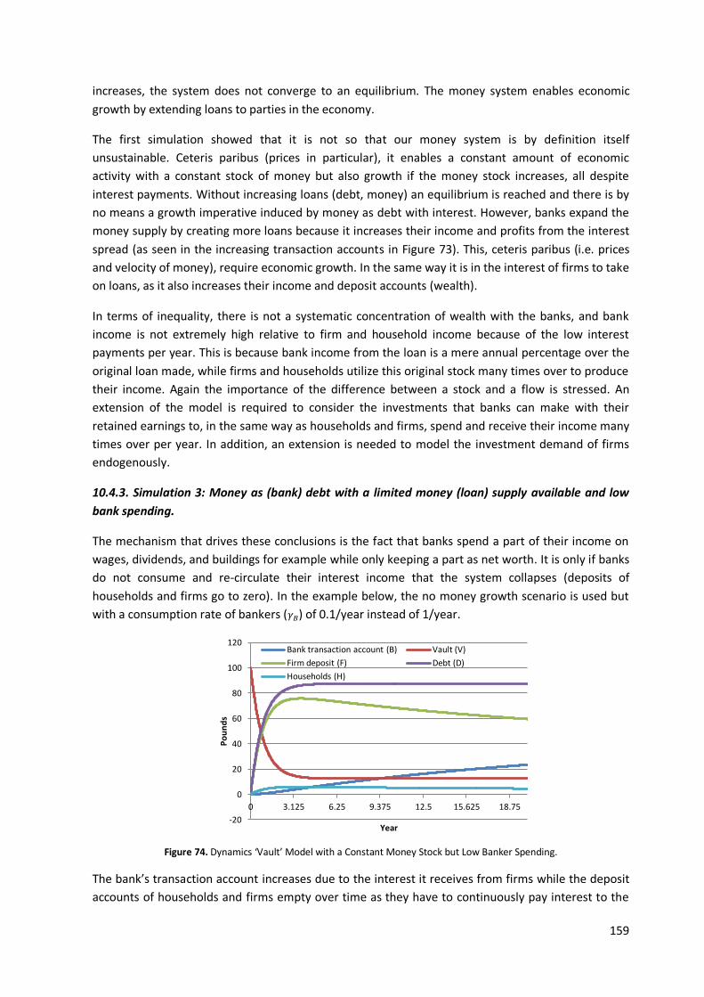
159

increases, the system does not converge to an equilibrium. The money system enables economic

growth by extending loans to parties in the economy.

The first simulation showed that it is not so that our money system is by definition itself

unsustainable. Ceteris paribus (prices in particular), it enables a constant amount of economic

activity with a constant stock of money but also growth if the money stock increases, all despite

interest payments. Without increasing loans (debt, money) an equilibrium is reached and there is by

no means a growth imperative induced by money as debt with interest. However, banks expand the

money supply by creating more loans because it increases their income and profits from the interest

spread (as seen in the increasing transaction accounts in Figure 73). This, ceteris paribus (i.e. prices

and velocity of money), require economic growth. In the same way it is in the interest of firms to take

on loans, as it also increases their income and deposit accounts (wealth).

In terms of inequality, there is not a systematic concentration of wealth with the banks, and bank

income is not extremely high relative to firm and household income because of the low interest

payments per year. This is because bank income from the loan is a mere annual percentage over the

original loan made, while firms and households utilize this original stock many times over to produce

their income. Again the importance of the difference between a stock and a flow is stressed. An

extension of the model is required to consider the investments that banks can make with their

retained earnings to, in the same way as households and firms, spend and receive their income many

times over per year. In addition, an extension is needed to model the investment demand of firms

endogenously.

10.4.3. Simulation 3: Money as (bank) debt with a limited money (loan) supply available and low

bank spending.

The mechanism that drives these conclusions is the fact that banks spend a part of their income on

wages, dividends, and buildings for example while only keeping a part as net worth. It is only if banks

do not consume and re-circulate their interest income that the system collapses (deposits of

households and firms go to zero). In the example below, the no money growth scenario is used but

with a consumption rate of bankers ( ) of 0.1/year instead of 1/year.

Figure 74. Dynamics ‘Vault’ Model with a Constant Money Stock but Low Banker Spending.

The bank’s transaction account increases due to the interest it receives from firms while the deposit

accounts of households and firms empty over time as they have to continuously pay interest to the

-20

0

20

40

60

80

100

120

0 3.125 6.25 9.375 12.5 15.625 18.75

Po

un

ds

Year

Bank transaction account (B) Vault (V)

Firm deposit (F) Debt (D)

Households (H)

160

bank without receiving enough money in return via bank spending. The money supply concentrates

itself with the bank in its transaction account (bank asset, not a deposit/liability). The ultimate result

is a collapse of the system as household and firm accounts can no longer finance their debts (firm

and household deposits go below zero, which is beyond the viable range set in the model). The

minimum consumption rate can be solved given the other parameters and a zero long-run

equilibrium deposit account for both banks and firm. This is a consumption rate equal to the interest

rate on loans ( ), here 0.08/year: at and below this banks consume too little to sustain a viable

economy because they spend into the economy less than they extract. Note that the necessary

consumption rate is not the interest rate spread, but the interest rate on loans, which is higher.

Of course the banks have no benefit of their income if they do not spend it, and therefore the system

will not necessitate instability or collapse. On the other hand, one could imagine that some sort of

sink exists outside of the general system to which banks channel their income and out of which they

spend. One could consider a sink of unproductive assets such as real estate, art, or increased

investments within the financial sector such as what has been seen in recent years (see Chapter 5) as

these reduce spending by the banks in the real economy – to firms and households. Increased capital

requirements for banks also result in earnings being retained and not reintroduced back into the

economy. Bezemer (2012) for example analyses the extent to which these trends occur and how this

has impacted the economy. Further research could undertake an extension of this simple model to

help illuminate the mechanisms at work in such a situation.

10.4.4. Simulation 4: A fixed loan supply and part ‘bank debt free’ money.

Finally, given the criticism on the necessity to pay interest over the entire money supply because all

money is (bank) debt, we here consider a situation in which there is an exogenous amount of money

( ) spent into the economy that is not complemented by an increase in the debt stock towards the

banks. The money is injected directly into the deposit accounts of households, paying civil servant

wages for example. The vault is again fixed at a constant amount that gradually is loaned into the

economy through firms. First, the results are given for a situation in which the available initial ‘bank

debt free’ money is one quarter of the total available loan stock: = ₤100 and a total of ₤25 is spent

into the system without increasing the total stock of loans. This is done at an exogenous spending

rate ( ) of 0.20/year so that all the available exogenous money ( ) is spent before year 20. The

change in the household deposit account is now given as follows:

(62)

(63)

The resulting equilibrium depends on the size of the exogenous expenditure (i.e. fraction of ‘debt

free’ money in the total money supply which includes also the loans from the vault) and not on the

rate of injection. Only the dynamics with which this equilibrium is reached depends on the speed at

which the money is spent into the household’s deposit. The general outcome in all situations is a (to

varying degrees) reduction in the equilibrium bank transaction account.

161

Figure 75. Dynamics ‘Vault’ Model with a Fixed Loan Supply and Part ‘Bank Debt Free’ Money.

The bank suffers from this expenditure because it has to pay deposit interest over it, but does not

receive loan interest in return. Its interest margin on this part of the money supply is the negative

deposit rate. Over time, the banks’ transaction account converges towards zero. Given these

parameter values, it is found that if an amount is injected that is greater than about 29% of the initial

vault level the transaction account of the bank tends to zero. Otherwise, it remains positive. A higher

borrowing rate or interest rate on loans increases this percentage because this increases the income

banks receive from loans while a higher repayment rate or interest rate on deposits decreases the

amount of exogenous money that causes the bank’s deposit to fall to zero. In sum, the simulation

reveals that the system dynamics change if not the entire money supply comes into existence

through a bank loan, in favor of households and firms and to the detriment of banks.

10.5. Conclusion.

The vault model is a useful tool to distinguish the stocks from the flows in the credit economy. It

enables one to consider the critique that the system is fallible because money is created as interest-

bearing bank debt, and more is requested in return (principal plus interest) than is loaned out

(principal). This dynamic analysis reveals that this does not imply an unviable system. It dispenses

with the popular beliefs that a growing money stock is required to sustain incomes and that the

system necessarily tends towards instability or collapse. A simple credit-economy can converge to a

steady-state if there is a fixed money supply. Loans from the vault function as a means of enabling

firm production, but as the net growth rate of loans decreases to zero, ceteris paribus (prices and

circulation velocity), the economy converges to the steady-state and the deposit accounts and

incomes are in an equilibrium. However, the system is only viable if the bank consumption rate is

greater than the interest rate that they earn on loans. Furthermore, a positive money creation rate,

ceteris paribus, enables (does not drive) growth in incomes and deposits accounts. Finally, being able

to create money yields indirect advantages for the banks as compared to the situation in which the

total money supply is a result of a bank loan. Basic differences in income between the classes in the

model however indicate that banks will not capture an excessive share of total income. While this

model can test for inherent mechanisms or biases in the system, it remains a very basic model. In

terms of absolute values and behavior it is fully dependent on exogenous initial parameter values.

Chapter 10 will therefore expand it to more explicitly include inequality and growth effects as well as

other economic indicators such as employment and inflation.

0

0.5

1

1.5

2

2.5

3

3.5

4

4.5

5

0

20

40

60

80

100

120

0 3.125 6.25 9.375 12.5 15.625 18.75

Po

un

ds

Po

un

ds

Year

Vault (V)

Firm deposit (F)

Debt (D)

Households (H)

'Debt free' money in the economy

Bank transaction account (B) (right axis)

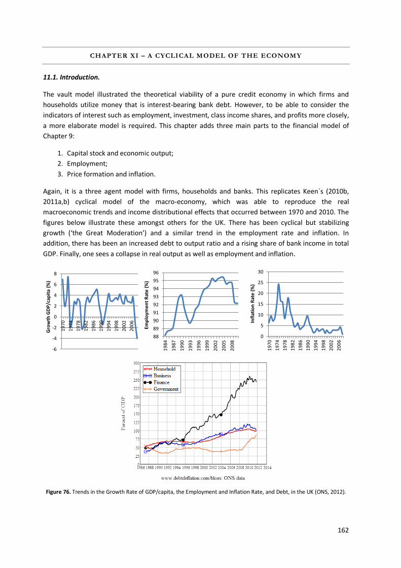
162

CHAPTER XI – A CYCLICAL MODEL OF THE ECONOMY

11.1. Introduction.

The vault model illustrated the theoretical viability of a pure credit economy in which firms and

households utilize money that is interest-bearing bank debt. However, to be able to consider the

indicators of interest such as employment, investment, class income shares, and profits more closely,

a more elaborate model is required. This chapter adds three main parts to the financial model of

Chapter 9:

1. Capital stock and economic output;

2. Employment;

3. Price formation and inflation.

Again, it is a three agent model with firms, households and banks. This replicates Keen´s (2010b,

2011a,b) cyclical model of the macro-economy, which was able to reproduce the real

macroeconomic trends and income distributional effects that occurred between 1970 and 2010. The

figures below illustrate these amongst others for the UK. There has been cyclical but stabilizing

growth (‘the Great Moderation’) and a similar trend in the employment rate and inflation. In

addition, there has been an increased debt to output ratio and a rising share of bank income in total

GDP. Finally, one sees a collapse in real output as well as employment and inflation.

Figure 76. Trends in the Growth Rate of GDP/capita, the Employment and Inflation Rate, and Debt, in the UK (ONS, 2012).

-6

-4

-2

0

2

4

6

8

19

70

19

74

19

78

19

82

19

86

19

90

19

94

19

98

20

02

20

06

Gro

wth

GD

P/c

apit

a (%

)

88

89

90

91

92

93

94

95

96

19

84

19

87

19

90

19

93

19

96

19

99

20

02

20

05

20

08

Emp

loym

en

t R

ate

(%

)

0

5

10

15

20

25

30 1

97

0

19

74

19

78

19

82

19

86

19

90

19

94

19

98

20

02

20

06

Infl

atio

n R

ate

(%

)

163

In the model, this collapse is caused by a cyclical but growing debt level which at a certain point is no

longer financeable for firms. This results in deleveraging since bankruptcy is not modeled, and

economic breakdown.

As introduced, Keen’s efforts are based on Goodwin’s (1967) growth cycle model rather than the

traditional equilibrium models of the economy. Goodwin developed a model based on the

employment rate and the share of wages in total output (Phillips curve). The oscillations are a result

of the multiplication of the wage rate and the level of employment. A high investment level causes

growth resulting in a decrease in unemployment, higher wages and a lower profit share, which

subsequently causes investment to decrease, followed by lower growth and a rise in unemployment

which lowers wages ultimately increasing the profit share again to repeat the cycle.

Keen alters this model slightly however, by “replacing the unrealistic assumption that capitalist invest

all their profits with the realistic nonlinear proposition that they invest more during booms and less

during slumps—with the variation accommodated by a financial sector that lends money at interest”

(Keen, 2010b). This is based on the observations of Keynes (1936) that under uncertainty, “the

present is a much more serviceable guide to the future than a candid examination of past experience

would show it to have been”. High current profit rates will thus be associated with higher rates of

investment compared to low profit rates. For the same reason Keen imposes a non-linear Phillips

curve that enables wages to increase faster at low unemployment rates and decrease slower at

higher levels of unemployment. The general exponential function that is utilized to do so is given

below. So while the psychology underlying the “euphoric” behavior described in Minsky’s Financial

Instability Hypothesis (1982) is not endogenously modeled, it is mimicked in the model through

nonlinear investment, wage and repayment functions that make the investment rate, growth rate of

the money (loan stock), rate of loan repayment, and the rate at which money circulates becomes

(nonlinearly) dependent on the profit rate.

The combination with the vault model makes this an explicitly monetary model. However, the ‘vault’

itself is removed, modeling money creation as the endogenous result of an increase in bank debt

held by firms for investment purposes. Money is recorded as a loan on the one hand, and an increase

in the firm’s deposits on the other as in the vault model, but now the change in debt is related to

investment behavior. Including prices together with the basic structure of the vault model allows for

a monetary system with a financial sector that is coupled with physical production.

The goal of this chapter is to apply Keen’s (2009, 2010a) model to consider potential effects that the

money system has on sustainable development. The model was chosen as an alternative model of

the economy to traditional models, which do not as explicitly consider the role of money, debt and

banks in the economy. To be able to apply it, Keen’s model is first extensively presented in the hope

of providing the reader with a general understanding of its structure. Note the model I have utilized

does not include speculation and ponzi-financing as Keen does in some of his extensions. The first

simulation that is presented is with Keen’s basic model (2009, 2010a). This is a base run, which I have

altered four times in additional simulations to explore the relationship with sustainable

development, given the role of the money system in the model. These four simulations no longer

follow Keen; they are my extensions. As stated, the model remains in its infant stages and requires

an elaborate sensitivity analysis, further research, and improvement. Nevertheless, it enables a first

attempt at understanding the relationship between sustainable development and the money system.

164

11.2. Model structure.

Figure 77 provides a simplified visual representation of the model. The colored area highlights the

link to the ‘vault’ model in the previous chapter. This stylized figure is followed by a more detailed

description of its various components. Please note that the letters that define each concept have

been chosen to best illustrate it and upper/lowercase letters are not necessarily related to stocks or

flows. The arrows are thus also not representations of flows but merely depict the main general

relationships in the model so to visualize its structure without presenting the full VensimTM model.

the exact relations follow.

Figure 77. Stylized Representation of the Cyclical Model.

CAPITAL STOCK ( )

capital/output

ratio ( )

labor productivity ( )

ANNUAL OUTPUT

( )

EMPLOYMENT

RATE ( )

LABOR FORCE

EMPLOYED ( )

PROFIT RATE ( )

FIRM LENDING

INVESTMENT ( )

FIRM ( ) DEPOSIT

ACCOUNT

LOAN REPAYMENT

HOUSEHOLD ( )

DEPOSIT ACCOUNT BANK ( )

DEPOSIT ACCOUNT

change in money

wages ( )

TOTAL MONEY

WAGES ( )

investment

function ( )

total labor force ( )

interest payments

to/from firms

( / )

wages ( )

repayment

function ( )

Interest payments / and

bank consumption ( )

interest to

households ( )

Household

consumption ( )

165

1. The basis of the model is a production system where output flow per year ( ) is related to the

capital stock ( ) through the capital-output ratio ( ) and to the stock of labor ( ) through a labor

productivity parameter ( ). There is technical change which results in an increase in the productivity

of labor at the exogenous rate ( ). Capital productivity ( ) is a constant exogenous variable

(calibrated below), equal to the amount of capital required for a unit of output.

(64)

(65)

(66)

2. Dividing this stock of labor ( ) by the total population ( ), yields the employment rate ( ). In

addition, the total population grows at an exogenous rate ( ).

(67)

(68)

3. The employment rate ( ), together with a number of other factors explained below determines the

rate of change in money wages per laborer (

). The equation given below is in line with Phillips

(1958) who, as stated next, identified three factors that affect the rate at which money wages

change: the “highly non-linear” relation between the rate of change of unemployment and money

wages given by the Phillips curve , “the rate of change of the demand for labor, and so of

unemployment” given by

, and “the rate of change of retail prices, operating through

cost of living adjustments in wage rates” given by

.

(69)

These components are:

a. A generalized exponential Phillips curve ( ) where is the argument. The function models a

nonlinear relationship between the employment rate ( ) and annual rate of change in money wages

per laborer (

). This equation is based on the equilibrium employment rate ( ) and the

associated equilibrium annual rate of change in money wages per laborer ( ), together with the

of the function at this point, and the minimum ( ) value of the function. The

parameterization in the following section provides more insight into this function.

(70)

b. A weighting factor ( ) that indicates the effect of changing the employment rate on the

wage rate.

c. The rate of change of the employment rate:

166

) (71)

is a function of the real growth rate of the economy ( , defined below), the exogenous change in

labor productivity ( ), and the population growth rate ( ).

d. The price level ( ) depends on price level equilibration, which is based on actual price setting

behavior (see Blinder, 1998) that the majority of firms apply cost-plus price setting behavior.

Therefore, they are modeled as a “markup over the monetary cost of production [here only

monetary wages], where the markup factor ( ) is equivalent to the equilibrium workers’ share

of real output” (Keen, 2010b) given by

. Note that

is used in the equation below. Prices are set

such that in equilibrium, the physical output equals monetary demand divided by the price level (see

Keen, 2010b for a derivation). The rate of change of the price level is subsequently modeled

assuming that prices converge over time to their equilibrium at a rate . This price setting

parameter, , represents the rate at which firms alter their prices. If it equals one for example, firms

immediately alter their prices while if it is less than one, firms take more than one time step to do so

and therefore the rate of change in the general price level is slower.

(72)

5. The total money wage bill ( ) equals the total labor force ( ) employed times the money wage

rate per laborer ( ).

(73)

6. The economy’s total nominal output ( ) per unit of nominal capital ( ) minus the income

of households and banks yields the profit rate ( ) in the economy. The income of households is the

total money wage bill ( ) and bank income equals ( ). Net interest is thus interest received on

firm deposits minus interest to be paid on loans.

(74)

7. The annual flow of firm investment ( ) depends on the profit rate through a general exponential

investment function that gives the investment rate as a function of the profit rate ( ) of firms.

Here again the functional form is such that the at the given equilibrium profit ( ) and

investment rates ( ) is exogenous, as is the minimum of the function ( ).

(75)

8. With firm investment we are back at the capital stock ( ) of the economy. It increases the stock,

while depreciation decreases it by an exogenous rate ( ).

(76)

9. The growth rate of the economy ( ) is a function of the investment rate ( ), the capital-output

ratio ( ) and the depreciation rate ( ).

167

(77)

10. In (7) the firms invest (a part of) output via its profits. The full money supply is bank debt.

Investment beyond a firm’s retained earnings results in the accumulation of long-term debt. This is

where the model links back to the basic vault model. Firm investment ( ) determines the total value

of loans or debt ( ) in the economy given the profit rate following Fama and French (1999): “debt

plays a key role in accommodating year-by-year variation in investment” and “more investment

tends to generate more debt, while higher earnings are used to reduce debt”. Note that this does not

even consider the psychological mechanisms of Minsky that are based on speculative expectation-

induced booms and busts.

In the model, any repayment of loans by firms reduces the stock of debt. Repayment is done as a

fraction of the firms’ deposit accounts ( ), which is also dependent on the profit rate through a non-

linear function ). Again, the minimum of the function is given by , is the natural repayment

rate (in equilibrium) that corresponds with the equilibrium profit rate, and the at this point is

also exogenous.

(78)

11. The debt in the economy ( ) needs to be serviced by the firms at a certain interest rate ( )

providing bank income to its transaction account ( ). Like in the vault model firm deposits ( ) as well

as household deposits ( ) receive interest at an interest rate from the bank.

(79)

(80)

(81)

12. The wages in the vault model are here equal to the wage bill ( ), while household ( ) and

banker ( ) consumption remains as it was in the vault model: dependent on the respective deposit

accounts ( and ) by an exogenous consumption rate ( and ).

(82)

(83)

168

11.3. Calibration.

The model is simulated using the following initial and parameter values. Again, this is based on Keen

(2010b, 2011a).

The Phillips curve ( ) in equation 70 above is based on the average long-run UK NAIRU4 of 4%

(Turner et al., 2001; Stock and Vogler-Ludwig, 2010) so at an equilibrium employment rate of 96%

wages do not change ( ). Furthermore, at this point the slope of the curve equal two, and

wages do not fall at a rate beyond a minimum rate of 4% when unemployment is high. This yields:

(84)

The figure below gives the resulting equation for the given parameter values.

Figure 78. Phillips Curve Factor as a Function of the Employment Rate.

The investment rate that results from the function is multiplied with real output to determine

the flow of investment (equation 75). It is simulated following Keen (2010b, 2011a) such that at an

equilibrium/natural profit rate of 4%, also 4% of economic output ( ) is invested. At a lower profit

rate less is invested, and at a higher profit rate more. The slope of the exponential at this point is 2,

and the fraction of output invested cannot be less than 0.

(85)

The figure below provides the resulting function based on these parameter values.

4 Non-Accelerating Inflation Rate of Unemployment, a concept similar to the natural rate of unemployment

because at this point inflation does not increase.

-0.1

-0.05

0

0.05

0.1

0.15

0.2

0.25

0.3

70.0

%

73.0

%

76.0

%

79.0

%

82.0

%

85.0

%

88.0

%

91.0

%

94.0

%

97.0

%

100.

0%

An

nu

al C

han

ge in

Rea

l Wag

e

(%)

Employment Rate

169

Figure 79. Investment Fraction as a Function of the Profit Rate.

The repayment rate presented in equation 78 that results of the repayment function ( ) is

parameterized in the same way that Keen (2010b, 2011a) does:

(86)

This entails that at an equilibrium profit rate of 4% firms allocate one tenth ( ) of their deposit

accounts to repay their loans. At this point the slope of the function is one ( ).

Furthermore, the function has a minimum repayment rate of 3% ( ). The division by 100 is to

convert between the values utilized in the model and the more understandable ‘rate’ representation.

The figure below provides the resulting function. When firms make more profits they use more of

their retained earnings that are in their deposit accounts to repay their loans, and when their profit

rate is lower they utilize a lower fraction of their deposit account to repay their debt. The figure gives

the actual repayment rate in percentage form (fraction of firm deposit), not the values used in the

model (multiply by 100).

Figure 80. Loan Repayment Rate as a Function of the Profit Rate.

0

0.05

0.1

0.15

0.2

0.25

0.3

0.35

1.0%

1.5%

2.0%

2.5%

3.0%

3.5%

4.0%

4.5%

5.0%

5.5%

6.0%

6.5%

7.0%

7.5%

8.0%

Inve

stm

en

t Rat

e (%

of

GD

P)

Profit Rate

0

0.02

0.04

0.06

0.08

0.1

0.12

0.14

0.16

0.18

0.2

1.0

%

1.5

%

2.0

%

2.5

%

3.0

%

3.5

%

4.0

%

4.5

%

5.0

%

5.5

%

6.0

%

6.5

%

7.0

%

7.5

%

8.0

%

Rep

aym

ent R

ate

(%)

Profit Rate

170

The following table provides a summary of the other parameters applied in the simulation as in Keen

(2011a). Given it is not the goal of this thesis to defend the model but rather to apply it, these values

are utilized in the following simulations. A brief discussion below does consider the main values.

However, it must be emphasized that an extensive sensitivity analysis is required for any further

extension of this work as the results are highly dependent on the model’s calibration.

Variable / parameter Description Value

Capital/output ratio 3

Labor productivity growth rate 2%/year

Population growth rate 1%/year

Depreciation rate 1%/year

Weighting factor that indicates the effect of a change in the employment rate on wage setting

0.1

Time constant for price setting 1

Markup coefficient 0.2

s.t.

= 1.25

and Consumption rate households and bankers

Initial values of the money wage level, labor productivity, total population, capital stock, economic output and price level.

1, 1, 300, 900, 300, 1

Loan and deposit interest rates. 6%/year, 2%/year

Initial values of the stock of loans or debt in the economy, firm and household deposit accounts, and bank transaction account.

0, 0, 0, 0

Table 15. Simulation Values Cyclical Model of the Economy.

The capital/output ratio across countries in 2007 was generally between two and three (Dobbs et al.,

2010). The value of three applied here is thus slightly high, in other words: true productivity of capital

is slightly better at on average 2.53. The UK even lies below this average at about 2.2. indicating

further that the value could have been altered downwards for application purely to the UK. Growth

rates of labor productivity vary quite significantly between countries but for the UK have indeed

been on average 2% since 1990 (OECD, 2012). The population growth rates of most Western

countries are between 0 and 1%, where in the UK it has been rising to about 0.7% in 2011 (World

Bank, 2012b). The depreciation rate of 1% utilized here is far below the average rate generally

utilized for developed countries between 5 and 6% (Dobbs et al., 2010; Schündeln, 2012). Since this is

such a large discrepancy, an increase in this rate is considered. It is found that this mainly speeds up

processes and does not alter the general outcome. Again, to stay in line with Keen’s original model

his parameterizations are maintained.

In sum, the parameter values applied in the model generally match those that have been empirically

established; however, there are clear differences over time and across countries which are beyond

the scope of this analysis. In the same way an extensive sensitivity analysis is not undertaken, as the

main goal of this chapter is to apply the model built by Keen to evaluate the effects it reveals on

sustainable development. The simulations that follow will reveal these basic tendencies that exist in

171

the system. In general, one sees that real economic output increases in a weakly cyclical manner

caused by debt-funded firm investments.

11.4. Simulations.

This section provides the results of five separate simulations. First, the basic model’s results are

presented. The deposit accounts of the three agents are no longer the most interesting variables to

consider. In all simulations trends in at least the following variables are rather provided: the

economy’s output and its growth rate, the employment and inflation rate, the debt to output ratio,

(firm) profit rates, and the income/output shares of the three agents. The latter is considered to

determine the income dynamics in the model to diagnose any systematic trends in inequality. While

sixty years are generally presented, a longer period of time has always been checked. In the first

basic model there is cyclical but stabilizing economic output, associated with a rising debt burden,

which eventually results in a collapse in the growth rate of the economy. To delve further into the

dynamics of the system and find ways to stabilize it and avoid the point of collapse, four alternative

simulations are provided that each hypothesize a ‘solution’.

The second simulation again considers the injection of money into the system without there being a

complementary increase in the total debt stock (e.g. government spending / ‘bank debt free’

money). In the previous chapter this stock of money that was not associated with an interest-bearing

loan had a detrimental effect for the banking sector. Here we also consider whether such exogenous

spending can prevent an economic collapse. Third, the impact of a more competitive banking sector

is simulated by reducing the interest spread that the banks earn. Fourth, we investigate whether a

lower propensity to invest may stabilize the system, based on the observation that it is investment

spending that results in lending and a rising debt burden. Finally, a situation of zero growth is

considered by reducing the labor and capital productivity growth rates to zero based on Daly’s (2010)

claim that a steady-state economy (recall this form of a steady-state entails zero not constant

growth) is needed.

11.4.1. Simulation 1 (Base Run): Cyclical model of the economy with money as (bank) debt.

This section presents the results of the model as it is outlined and calibrated above. UK actual values

of the Great Moderation and the period just before are presented also as these reflect the time

period of interest that led up to the recent crisis. The result is cyclical and stabilizing economic

growth followed by a collapse. The figure below presents both the yearly level of economic output

and the annual growth rate. As stated, for comparison, the trends in economic growth in the UK from

1970 to 2007 are given also.

172

Figure 81. Annual Real Economic Output and Growth – Simulation 1 and UK Actual Values (ONS, 2012).

This simulation results initially in volatile economic output and growth. However, the cycle in the

level of economic output decreases in amplitude quickly (hardly noticeable in the figure) and tends

towards a positive linear trend. The changes in the growth rate also dampen and the economy seems

to converge to a growth rate of about 3%/year. The empirical UK trends reveal a similar high volatility

in the early 1970s, which stabilize from 1994 onwards also around 3% growth per year. Indicators of

economic prosperity such as employment and inflation rates replicate these initially positive trends.

Figure 82. Employment (top) and Inflation (bottom) Rates – Simulation 1 and UK Actual Values (ONS, 2012).

Initially, the employment rate drops but again the cycles diminish over time. The same trend is seen

in the inflation rate. There is a trend towards the exogenous equilibrium natural employment rate of

96% at which there is no change in wages. The inflation rate tends to zero and the price level (not

shown here) to just over three times its original level. Again the empirical rates in the UK are

provided also for comparison. These reveal similarly volatile employment and inflation rates in the

early 1970s followed by gradual stabilizing – upwards for the employment rate and downwards to

zero for the inflation rate. Between 2001 and 2006 the employment rate seems to have stabilized at

about 95% and the inflation rate around 2.5% for an ever longer period since 1994 already. The main

-2

0

2

4

6

8

10

12

14

0

200

400

600

800

1000

1200

1400

1600

0 5 10 15 20 25 30 35 40 45 50 55 60

Gro

wth

rat

e (

%/Y

ear

)

Re

al O

utp

ut

(Po

un

ds/

Ye

ar)

Year

Real output (level)

Growth rate real output

-6

-4

-2

0

2

4

6

8

19

70

19

74

19

78

19

82

19

86

19

90

19

94

19

98

20

02

20

06

Gro

wth

GD

P/c

apit

a (%

)

70

75

80

85

90

95

100

0 5 10 15 20 25 30 35 40 45 50 55 60

Emp

loym

en

t R

ate

(%

)

Year

88

89

90

91

92

93

94

95

96 1

98

4

19

87

19

90

19

93

19

96

19

99

20

02

20

05

20

08

Emp

loym

en

t R

ate

(%

)

-40

-30

-20

-10

0

10

20

30

40

50

60

0 5 10 15 20 25 30 35 40 45 50 55 60 Infl

atio

n R

ate

(%

)

Year

0

5

10

15

20

25

30

19

70

19

74

19

78

19

82

19

86

19

90

19

94

19

98

20

02

20

06

Infl

atio

n R

ate

(%

)

173

Figure 83. Debt to Output Ratio – Simulation 1.

difference is that in the model there are significant periods of deflation, while in the UK until the

crisis there has been mainly inflation. We also see a significant difference in the absolute values of

the inflation rate, where the model predicts unrealistically high inflation rates. This is one indication

that further research would require an improved calibration and examination of price formation in

the model. However, we are here mainly interested in the general trends than the absolute figures

which are purely dependent on initial parameter settings.

The cyclical nature of the economy in the model is a result of the investment function and the Phillips

curve due: the multiplication of the wage rate and the level of employment and the desire of firms to

lend and invest in relation to the profit rate respectively. The amplitude of the cycles decrease over

time and there is an indication of a Great Moderation. One is led to believe that the business cycle is

under control and the economy is prospering. However, in all these figures there is a collapse. Both

the collapse and the cyclical behavior are consequences of the fact that firms invest more when

profit rates are high, and less when these are low and that a similar trend occurs in employment:

wages increase faster at high rates of employment than that they fall at low rates of employment.

Close to collapse, first, inflation turns into persistent deflation and the price level falls, followed later

by increased unemployment and a drop in real economic output after about year 50. This is a result

of the combination of a growing stock of debt and deflationary pressures. The real interest

requirements hereby remain low at first, but as the debt stock rises these increase over time creating

a burden on the economy. The figure below shows the sudden rapid increase in debt in the model.

Figure 84. Total Interest Paid on Loans by Firms and Firm Profit Rates – Simulation 1.

Compared to the growth rates in output, we see the debt level in the economy first increases over

time in a step-wise fashion where the level increases during a boom (growth in output) and falls

during a slump (with some lag time).

0

5

10

15

20

25

30

35

0 5 10 15 20 25 30 35 40 45 50 55 60

De

bt-

to-O

utp

ut

Rat

io

Year

-30

-25

-20

-15

-10

-5

0

5

10

15

0

500

1000

1500

2000

2500

3000

0 5 10 15 20 25 30 35 40 45 50 55 60

Pro

fit

Rat

e (

%)

Inte

rest

(P

ou

nd

s/Y

ear

)

Year

Real interest on loans

Firm profit rate

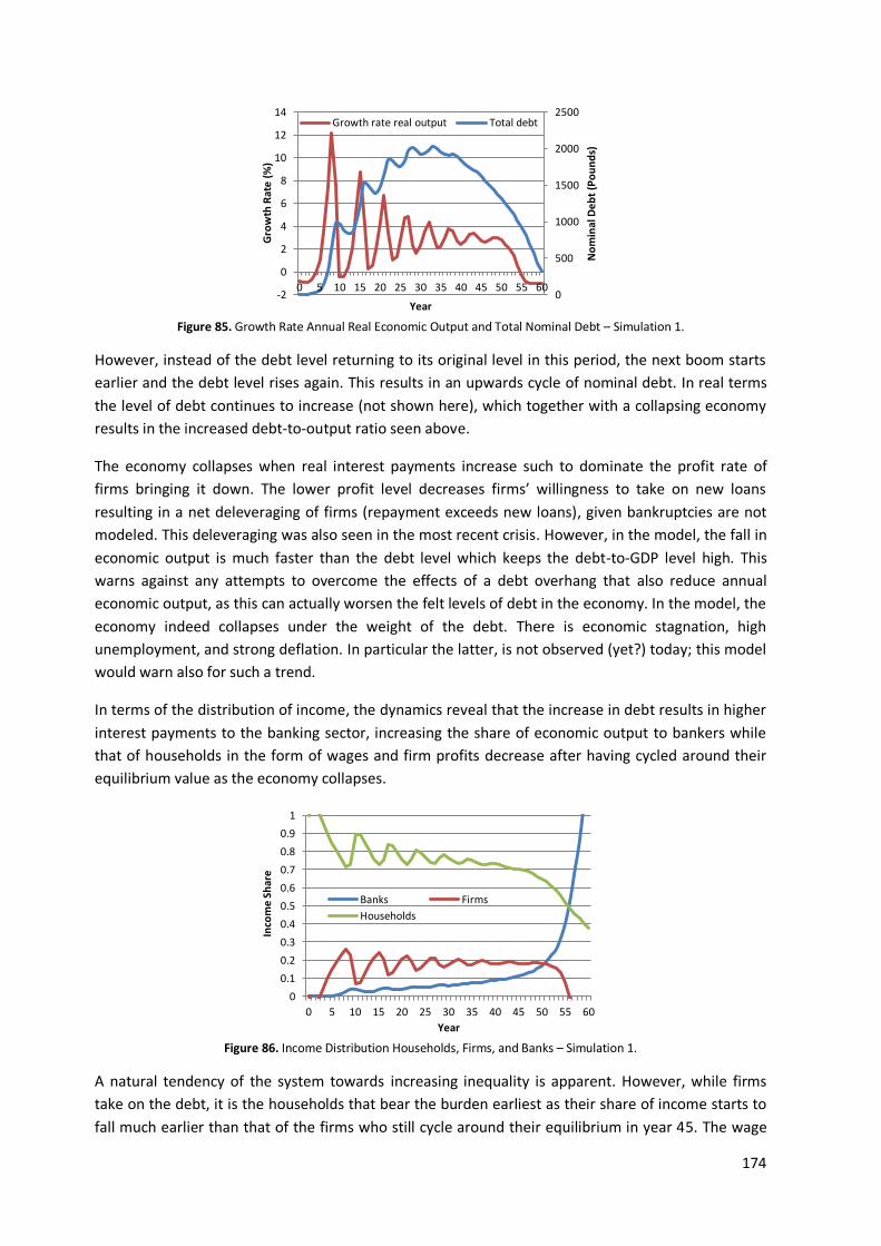
174

Figure 85. Growth Rate Annual Real Economic Output and Total Nominal Debt – Simulation 1.

However, instead of the debt level returning to its original level in this period, the next boom starts

earlier and the debt level rises again. This results in an upwards cycle of nominal debt. In real terms

the level of debt continues to increase (not shown here), which together with a collapsing economy

results in the increased debt-to-output ratio seen above.

The economy collapses when real interest payments increase such to dominate the profit rate of

firms bringing it down. The lower profit level decreases firms’ willingness to take on new loans

resulting in a net deleveraging of firms (repayment exceeds new loans), given bankruptcies are not

modeled. This deleveraging was also seen in the most recent crisis. However, in the model, the fall in

economic output is much faster than the debt level which keeps the debt-to-GDP level high. This

warns against any attempts to overcome the effects of a debt overhang that also reduce annual

economic output, as this can actually worsen the felt levels of debt in the economy. In the model, the

economy indeed collapses under the weight of the debt. There is economic stagnation, high

unemployment, and strong deflation. In particular the latter, is not observed (yet?) today; this model

would warn also for such a trend.

In terms of the distribution of income, the dynamics reveal that the increase in debt results in higher

interest payments to the banking sector, increasing the share of economic output to bankers while

that of households in the form of wages and firm profits decrease after having cycled around their

equilibrium value as the economy collapses.

Figure 86. Income Distribution Households, Firms, and Banks – Simulation 1.

A natural tendency of the system towards increasing inequality is apparent. However, while firms

take on the debt, it is the households that bear the burden earliest as their share of income starts to

fall much earlier than that of the firms who still cycle around their equilibrium in year 45. The wage

0

500

1000

1500

2000

2500

-2

0

2

4

6

8

10

12

14

0 5 10 15 20 25 30 35 40 45 50 55 60

No

min

al D

eb

t (P

ou

nd

s)

Gro

wth

Rat

e (

%)

Year

Growth rate real output Total debt

0

0.1

0.2

0.3

0.4

0.5

0.6

0.7

0.8

0.9

1

0 5 10 15 20 25 30 35 40 45 50 55 60

Inco

me

Sh

are

Year

Banks Firms

Households

175

share of income falls as the debt level increases, while the share of firm profits in total income

fluctuates at a steady level for much longer. It falls when banks’ share of income significantly rises.

This is made clearer by the wage and profit rates given below (household and firm income).

Figure 87. Wage and Profit Rates – Simulation 1.

The wage rate already starts to decrease quite significantly after year 25 while the profit rate remains

high for much longer. Nevertheless, both rates collapse because of the build-up of debt that is

associated with the role that the banks play in financing investment. The increase in the debt-GDP

ratio first results in a receding worker share in GDP, and firms follow, yielding to the debt servicing

requirements of banks. Keen (2010b) labels this ‘class conflict not between workers and capitalists

but between financial and industrial capital’. The debt-induced breakdown causes income inequality.

11.4.2. Simulation 2: Cyclical model of the economy with money as (bank) debt plus (bank debt-

free) spending.

The basic simulation revealed that there was a tendency, given the initial parameter values, towards

stabilization but followed by economic collapse. In an attempt to understand what causes this

collapse, and search for manners to avoid this, a number of simulations are undertaken based on the

analysis of Parts I and II. The previous chapter already considered the argument that the current

money system is unviable because the entire money supply is associated with interest-bearing (bank)

debt. Therefore, one may hypothesize that the process of debt-deflation in the previous simulation

can be avoided through the injection of money that is not associated with a bank loan. For example,

a certain amount can be created and spent by the government yearly into the households’ deposit

account (e.g. civil servant wages or health and education benefits), but without the equal increase in

firm loans that is associated with the usual increase in the money supply. This may act as a stabilizing

force. Since government debt is not modeled here, it is assumed the government can as it were,

‘print’ money and spend it, or that it can build up a debt with no effect. In this simulation ₤500 is

added to the deposit account of households at a rate of 10%/year without a simultaneous increase in

the debt stock. As in the previous chapter, the equilibrium is not sensitive to the rate, this merely

alters the speed with which it is reached. Households now consume from firms and receive not only

wages and interest on their deposits, but also this extra amount per year. By modeling ‘bank debt

free spending’ in this manner the government/central bank can be abstracted from without altering

the result. The term ‘government’ is used here merely as an indication of a public institution that is

theoretically representative of the entire society. One can imagine this task to be allotted to the

central bank or another independent institution – important is that it is not influenced by politics. An

0

0.5

1

1.5

2

2.5

3

3.5

4

-30

-25

-20

-15

-10

-5

0

5

10

15

0 5 10 15 20 25 30 35 40 45 50 55 60

Wag

e R

ate

(%

)

Pro

fit

Rat

e (

%)

Year

Profit rate (firms)

Wage rate (households)

176

in depth exploration of such solutions go beyond the scope of this thesis but it is important to note

given the use of the term ‘government’.

The simulation reveals indeed that such spending avoids the collapse of the system. There is a steady

increase in economic output just under 3% per year, a stabilized employment rate slightly above the

natural rate of 96%, and a constant inflation rate. While sixty years are presented below, a longer

period of time was also checked to see whether the collapse was not simply delayed. This was not

the case, the equilibrium rates given below continue infinitely due to this exogenous ‘bank debt free’

injection of ₤500. Altering this value reveals that stability is reached if a minimum total of ₤220 is

spent.

Figure 88. Annual Real Economic Output and Growth – Simulation 2.

Figure 89. Employment and Inflation Rate – Simulation 2.

In the previous chapter such an injection had very negative effects for the banking sector because it

had to pay deposit interest over a stock of money that it did not receive loan interest over. To

consider whether this is again the case, the income shares of the three classes are given below.

-2

0

2

4

6

8

10

12

14

0

200

400

600

800

1000

1200

1400

1600

1800

2000

0 5 10 15 20 25 30 35 40 45 50 55 60

Gro

wth

rat

e (

%/Y

ear

)

Re

al O

utp

ut

(Po

un

ds/

Ye

ar)

Year

Real Output (level)

Growth Rate Real Output (%)

80

82

84

86

88

90

92

94

96

98

100

-40

-30

-20

-10

0

10

20

30

40

50

60

0 5 10 15 20 25 30 35 40 45 50 55 60 Emp

loym

en

t R

ate

(%

)

Infl

atio

n R

ate

(%

)

Year

Inflation Rate

Employment Rate

177

Figure 90. Income Distribution Households, Firms, Banks – Simulation 2.

Unlike before, the income shares (percent of GDP) remain stable in this situation. Households obtain

the largest share of economic output (tends to 76%), followed by the firms (tends to 18%), and then

banks (tends to 6%). The latter obtain only a very small share of income for the same reason as

outlined above: the interest they receive is a mere annual percentage over a total amount while

households and firms receive an income many times over per year. The mechanism towards

economic collapse is removed, as is the complementary increase in the income share of output of

banks.

The injection of money by the government in worker deposit accounts is able to stabilize the system

by adding money without interest associated with it. In this manner economic growth is funded with

new money that does not enter the economy as bank debt but through GDP enhancing government

spending. In terms of the economy’s debt burden, there remains a cyclical buildup of debt in the first

decades. However, now the firms are able increase or decrease their leverage without an economic

collapse and the debt-to-output ratio does not surpass 170%. Profit rates are able to stabilize around

6% since there remains an amount of money in the economy that was not associated with firm loans

and thus they are not overwhelmed by interest payments.

Figure 91. Debt-to-Output Ratio and Firm Profit Rate – Simulation 2.

Note that government debt is not modeled, which this exogenous spending also is, given all money is

essentially debt. However, this is debt that society ‘owes’ to itself and thus does not have the

concentrating effects of debt owed to a private sector in the economy. Theoretically (not modeled),

the two methods of money creation are different. While in the standard case money is allocated in

the first instance to firm investments, this second option spends money into the economy through

0

0.1

0.2

0.3

0.4

0.5

0.6

0.7

0.8

0.9

1

0 5 10 15 20 25 30 35 40 45 50 55 60

Inco

me

Sh

are

Year

Banks Firms Households

-0.2

0

0.2

0.4

0.6

0.8

1

1.2

1.4

1.6

1.8

0 5 10 15 20 25 30 35 40 45 50 55 60

De

bt-

to-O

utp

ut

Rat

io

Year

-4

-2

0

2

4

6

8

10

1 6 11 16 21 26 31 36 41 46 51 56 61

Pro

fit

Rat

e (

%)

Year

178

government (chosen) spending. This does not have to be additional spending, but a part of

government expenditure is not money in the form of bank debt. The potential implications of this are

discussed in a later section.

11.4.3. Simulation 3: Cyclical model of the economy with money as (bank) debt and increased

competition in the banking sector.

Chapter 5 revealed that the financial sector is becoming increasingly concentrated, as the top 3

banks in the UK own more than half the entire banking sector’s total assets. This entails more market

power over the interest rate spread (here 6% - 2% = 4%). In a perfectly competitive market this

spread would converge to a minimal amount equal to the marginal costs of the banks. However, in a

concentrated market, the monopolistic competitors are able to keep the interest spread high. By

exogenously altering the difference between the rate charged on loans and the rate paid on deposits

in the model the effects of such a change in market competition can be simulated. In the following

simulation, the model is reset to its original parameter settings, but with an interest rate on loans of

3%, yielding an interest rate spread of just 1% for the banks. The results are given in the figures

below. For a better illustration a longer time period is provided (100 years). Altering this value to test

the model’s sensitivity yielded that this stability resulted only for any spread between 0 and 2.8%.

Figure 92. Annual Real Economic Output and Growth – Simulation 3.

The cyclical behavior is clearly enhanced in this simulation. Economic output ratchets upwards

though the growth rate with which it does so diminishes over time. A longer time period reveals it

converges in the long-run to a growth rate of 3% and the volatility of the level of economic output is

reduced. Again, the main difference with the first simulation is that there is no crash in economic

output (also not in later years beyond this graph). The system rather converges to a stable

equilibrium. The employment rate and price level reveal a similar trend as seen in the following

figures.

-4

-2

0

2

4

6

8

10

12

14

16

18

0

200

400

600

800

1000

1200

1400

1600

1800

2000

0 5 10 15 20 25 30 35 40 45 50 55 60

Gro

wth

rat

e (

%)

Re

al O

utp

ut

(Po

un

ds/

Ye

ar)

Year

Real Output (level)

Growth Rate Real Output (%)

179

Figure 93. Employment and Inflation Rate – Simulation 3.

The employment rate converges to 97.2% (above its exogenously set natural level at which wages do

not change). The inflation rate tends to about 10%. Both rates are also highly volatile in the early

years but tend towards stabilization. Note that again the absolute values of the inflation rates are

very high. Any costs of inflation/deflation that are not modeled would likely come about at such

rates. This would alter the growth rate of the economy that is found here. Again, we are interested in

the general trend rather than the absolute values, which depend on the initial calibration.

The lack of debt-induced collapse means the income distribution is also not skewed towards bankers

in the long-run (Figure 94).

Figure 94. Income Distribution Households, Firms, and Banks – Simulation 3.

Rather, banks obtain only a small portion of GDP, about 1% in this simulation. The largest share of

GDP is captured by households, about 81% in the long-run, and firms capture the remaining 18%. The

lower interest spread is, as expected, seen back in a lower income share for banks.

Considering other interest rate spreads, a difference of 2% also yields a stabilized economy, but once

the spread increases to 3% the system again undergoes a debt-induced collapse in the long-run.

Stability is thus negatively related to the interest rate spread: there is increased stability under a

lower spread. Ceteris paribus, it is positively on the interest rate on deposits ( ) and negatively on

the interest rate on loans ( ). A high level of competition in the financial market, as represented by a

lower spread that commercial banks earn on the difference between loans and deposit interest

rates, stabilizes the system to a long-run equilibrium. Hence, active searching by banks to increase

60

65

70

75

80

85

90

95

100

-150

-100

-50

0

50

100

150

200

0 5 10 15 20 25 30 35 40 45 50 55 60

Emp

loym

en

t R

ate

(%

)

Infl

atio

n R

ate

(%

)

Year

Inflation Rate Employment Rate

0

0.1

0.2

0.3

0.4

0.5

0.6

0.7

0.8

0.9

1

0 5 10 15 20 25 30 35 40 45 50 55 60

Inco

me

Sh

are

Year

Banks Firms Households

180

their interest spread (e.g. by expanding abroad) causes instabilities in the system. However, a low

interest spread enables a rising stock of debt without diminishing the profit rate of firms.

Figure 95. Debt-to-Output Ratio and Firm Profit Rate– Simulation 3.

The rise in the debt-to-output ratio converges in the long-run to about 1.1 (110%). This level of debt

can apparently be taken on, held, and financed by firms because of the lower interest rate on loans.

The long-run inflation rate of 10% is also expected to play a role in enabling the payment of the debts

as it reduces the real debt burden in the economy. Profit rates are not pushed downwards by the

debt servicing costs and converge to a long-run rate just over 6%. The total stock of debt in the

economy does not decrease – firms take on more debt than they repay, which finances long-run

viable economic growth.

11.4.4. Simulation 4: Cyclical model of the economy with money as (bank) debt and a lower

propensity to invest.

Given the source of debt in the model is investment, requiring new loans and money creation, and a

high debt burden is seen to result in instability, one may hypothesize that less investment in the

economy can also result in stabilization. Figure 97 gives the economic growth rate and level of

economic output when the propensity for firms to invest has exogenously been reduced yielding a

lower rate of credit creation. This is done by altering the investment function (equation 85) so that a

smaller percentage of GDP is invested yearly:

(87)

Figure 96. Investment Fraction with a High (Base Run) and Low Propensity to Invest.

0

0.2

0.4

0.6

0.8

1

1.2

0 5 10 15 20 25 30 35 40 45 50 55 60

De

bt-

to-O

utp

ut

Rat

io

Year

-4

-2

0

2

4

6

8

10

1 6 11 16 21 26 31 36 41 46 51 56 61

Pro

fit

Rat

e (

%)

Year

-5

0

5

10

15

20

25

30

35

40

45

0 5 10 15 20 25 30 35 40 45 50

Inve

stm

en

t Fr

acti

on

(%

)

Year

Investment Fraction (Base Run)

Investment Fraction (Simulation 4)

181

The figures above show the difference between the original higher investment function where a

larger share of output was invested, versus the weaker investment function utilized in this

simulation. The lower propensity to invest results in a viable economy – stabilization without

collapse. The figures again show a time period of sixty years; however, it was checked for a longer

period and the collapse does not occur after year sixty either.

Figure 97. Annual Real Economic Output and Growth – Simulation 4.

The economy converges quite quickly to a steady growth rate of 3%. The cycles in economic output

dampen and real output steadily increases. The model economy tends towards a long-run

employment at about 96.5%.

Figure 98. Employment and Inflation Rate – Simulation 4.

The inflation rate seems to converge to a very high 25%; however, extending the time period reveals

that it starts to cycle upwards after year ninety. Nevertheless, there is no economic collapse in these

years beyond those given above. The periods of alternating inflation and deflation seen here are

followed solely by ever increasing inflation. This enables the debt-to-output ratio to stabilize (around

90% of GDP) as seen in the next figures.

-1

0

1

2

3

4

5

6

7

8

9

0

200

400

600

800

1000

1200

1400

1600

1800

2000

0 5 10 15 20 25 30 35 40 45 50 55 60

Gro

wth

rat

e (

%)

Re

al O

utp

ut

(Po

un

ds/

Ye

ar)

Year

Real Output (level)

Growth Rate Real Output (%)

60

65

70

75

80

85

90

95

100

-200

-150

-100

-50

0

50

100

150

200

250

0 5 10 15 20 25 30 35 40 45 50 55 60

Emp

loym

en

t R

ate

(%

)

Infl

atio

n R

ate

(%

)

Year

Inflation Rate Employment Rate

182

Figure 99. Debt-to-Output Ratio and Firm Profit Rate – Simulation 4.

The inflation decreases the debt burden, which enables a rising stock of debt without negative

economic consequences. The profit rate of firms seen above stabilizes to a positive five percent in

the long-run. However, the negative effects of high inflation or deflation rates are not modeled (see

e.g. Blanchard, 2011 for the costs of deflation and inflation). These may have economic

consequences that alter consumer and firm behavior in such as way that is not modeled here. This

analysis is beyond the scope of this thesis but does require further research.

The shares in output of the three agents are also seen to stabilize as before, with households

obtaining the largest share – about 80% in the long-run, followed by firms (16%) and banks (4%).

Figure 100. Income Distribution Households, Firms, and Banks – Simulation 4.

A lower propensity to invest removes the tendency towards collapse in the system. The debt burden

rises but only slowly. Perhaps this is only possible in the long-run because of the high inflation rate,

which is induced by a higher money wage rate (following growing labor productivity). Since the

negative effects of inflation are not modeled the true socio-economic ramifications cannot be made

explicit. This simulation thus requires further consideration and an elaboration of the model that is

beyond the scope of this thesis.

0

0.2

0.4

0.6

0.8

1

1.2

0 5 10 15 20 25 30 35 40 45 50 55 60

De

bt-

to-O

utp

ut

Rat

io

Year

-6

-4

-2

0

2

4

6

8

10

0 5 10 15 20 25 30 35 40 45 50 55 60

Pro

fit

Rat

e (

%)

Year

0

0.1

0.2

0.3

0.4

0.5

0.6

0.7

0.8

0.9

1

0 5 10 15 20 25 30 35 40 45 50 55 60

Inco

me

Sh

are

Year

Banks Firms

Households

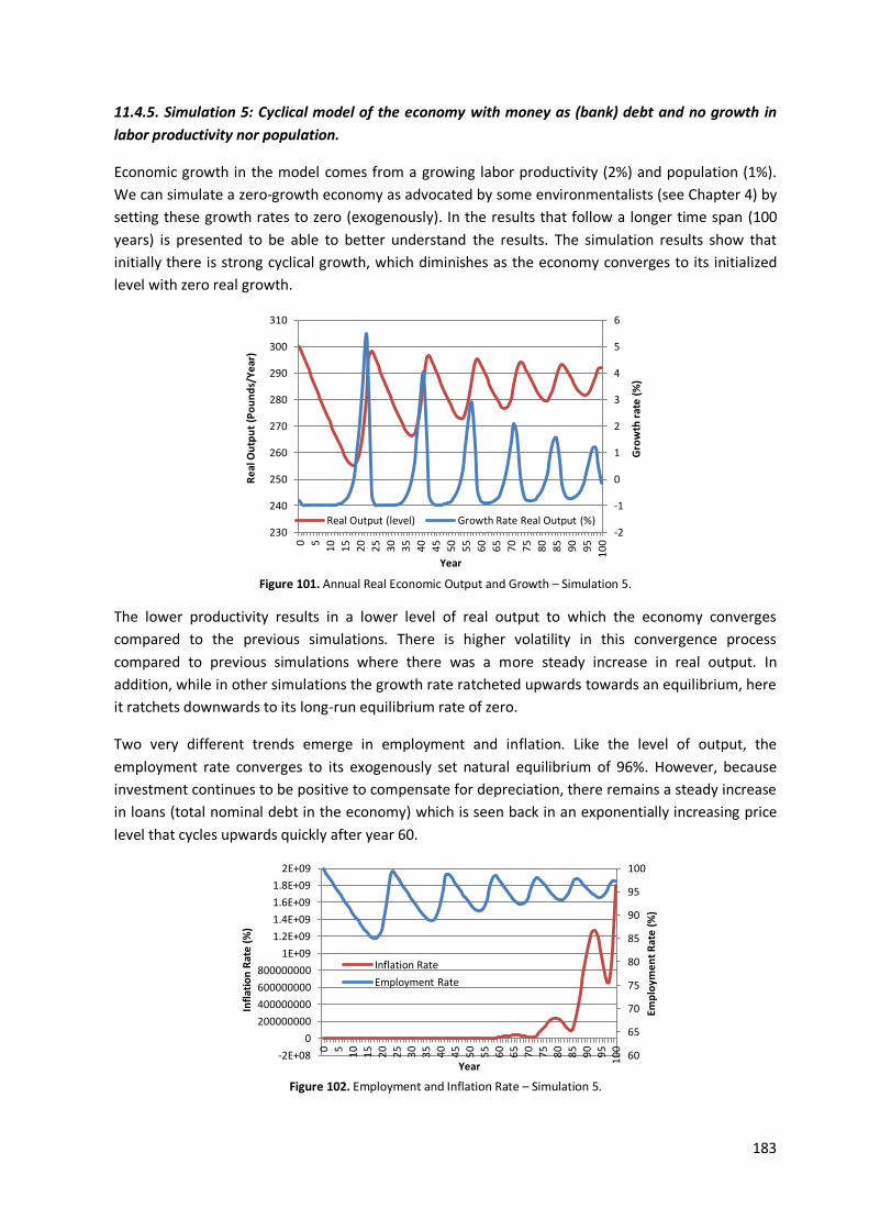
183

11.4.5. Simulation 5: Cyclical model of the economy with money as (bank) debt and no growth in

labor productivity nor population.

Economic growth in the model comes from a growing labor productivity (2%) and population (1%).

We can simulate a zero-growth economy as advocated by some environmentalists (see Chapter 4) by

setting these growth rates to zero (exogenously). In the results that follow a longer time span (100

years) is presented to be able to better understand the results. The simulation results show that

initially there is strong cyclical growth, which diminishes as the economy converges to its initialized

level with zero real growth.

Figure 101. Annual Real Economic Output and Growth – Simulation 5.

The lower productivity results in a lower level of real output to which the economy converges

compared to the previous simulations. There is higher volatility in this convergence process

compared to previous simulations where there was a more steady increase in real output. In

addition, while in other simulations the growth rate ratcheted upwards towards an equilibrium, here

it ratchets downwards to its long-run equilibrium rate of zero.

Two very different trends emerge in employment and inflation. Like the level of output, the

employment rate converges to its exogenously set natural equilibrium of 96%. However, because

investment continues to be positive to compensate for depreciation, there remains a steady increase

in loans (total nominal debt in the economy) which is seen back in an exponentially increasing price

level that cycles upwards quickly after year 60.

Figure 102. Employment and Inflation Rate – Simulation 5.

-2

-1

0

1

2

3

4

5

6

230

240

250

260

270

280

290

300

310

0

5

10

15

20

25

30

35

40

45

50

55

60

65

70

75

80

85

90

95

10

0

Gro

wth

rat

e (

%)

Re

al O

utp

ut

(Po

un

ds/

Ye

ar)

Year

Real Output (level) Growth Rate Real Output (%)

60

65

70

75

80

85

90

95

100

-2E+08

0

200000000

400000000

600000000

800000000

1E+09

1.2E+09

1.4E+09

1.6E+09

1.8E+09

2E+09

0

5

10

15

20

25

30

35

40

45

50

55

60

65

70

75

80

85

90

95

10

0

Emp

loym

en

t R

ate

(%

)

Infl

atio

n R

ate

(%

)

Year

Inflation Rate

Employment Rate

184

Again, the consequences of inflation for society are not modeled and therefore there are no negative

implications of this situation. The inflation rate that emerges is clearly unsustainable, but in this

model it has no effect. The expanding money supply (nominal debt) is able to complement zero-

growth. The high inflation rate stabilizes the debt-to-output ratio to just 15% in the long-run.

Figure 103. Debt-to-Output Ratio – Simulation 5.

With this result it seems that a growing labor productivity and population increase the need for

credit to fund the resulting economic growth. This increases the stock of debt, which can destabilize

the system if the debt burden becomes too high. However, without the pressure of productivity and

population growth, less credit is demanded (only to replace depreciated capital), and a lower debt-

to-output ratio results. The trend in the price level enables such a low level of debt-to-output as any

increase in nominal debt reveals itself in the price level, attaining no real income growth in the long-

run. In this simulation, income shares also stabilize.

Figure 104. Income Distribution Households, Firms, and Banks – Simulation 5.

In the long-run, households obtain the highest share of economic output (90%), followed by firms

(9%). Bankers receive about 1% in this zero-growth scenario because of the low levels of debt. In

addition to the limitation of the model in terms of inflation, one can also question how realistic zero

labor productivity and population growth is. These limitations are considered more in the following

chapter. Nevertheless, we find only a growing economy requires a growing money supply. By

removing this growth (labor productivity and population) the economic collapse is avoided in the

model. As predicted in the ‘old view’, monetary expansion merely results in inflation. This

inflationary result hints at an overlap and complementary characteristics between the ‘old’ and ‘new’

view. This will also be discussed in the next (conclusion and discussion) chapter more extensively.

0

0.1

0.2

0.3

0.4

0.5

0.6

0

5

10

1

5

20

2

5

30

3

5

40

4

5

50

5

5

60

6

5

70

7

5

80

8

5

90

9

5

10

0

De

bt-

to-O

utp

ut

Rat

io

Year

0

0.1

0.2

0.3

0.4

0.5

0.6

0.7

0.8

0.9

1

0

5

10

1

5

20

2

5

30

3

5

40

4

5

50

5

5

60

6

5

70

7

5

80

8

5

90

9

5

10

0

Inco

me

Sh

are

Year

Banks Firms

Households

185

11.5. Discussing the implications for sustainable development.

This model of Keen reveals the basic dynamics of a credit economy, in which interest-bearing bank

debt circulates as money. The short-run reveals positive trends in economic indicators which seem

encouraging. However, in the base run these eventually give way to destabilization and a situation of

debt induced deflation and economic collapse as long as the driving forces of productivity and

population growth exist. The system has a stable long-run equilibrium under a portion of ‘bank debt

free’ (government) spending, a lower propensity to invest or a lower interest spread. Even then,

however, the rising labor productivity still has the effect of encouraging economic growth which, as

seen in Part I, has until today had negative effects on the environment. The opportunities for other

more sustainable growth paths is considered in the following conclusion and discussion chapter. The

system is thus not by definition instable, and it does not impose a growth imperative on the economy

in itself. The dynamics that are more extensively revealed in this chapter, indicate that given the

behavior of the agents in the system, it does have implications for sustainable development.

The model reveals that the buildup of debt may initially have positive effects on the economy and

society, but that it is unsustainable in the long-term. Even in the short-run, the cyclical nature of the

credit economy results in under- and over-allocation of resources. During economic booms resources

are underutilized, while during busts the capital that remains from the bust is in excess of what is

needed and is underutilized. Although these cycles decrease in amplitude in the model, at some

point the interest payments on the growing debt burden start to dominate profit rates. Theoretically,

firms rather deleverage in this situation, and in the model repayment rates start to exceed new loan

(investment) rates. These processes ultimately give rise to a breakdown of the system if there is no

intervention. There is a negative result for two pillars of sustainable development as in the long-run

income inequality automatically increases and economic progress comes to a standstill. Of course,

this lack of economic growth may have benefits for the environment; however, a sustainable system

was defined as one in which all three pillars are viable.

One way to establish stability in the system was ‘government’ spending. This required injecting a

portion of money into the system that was not associated with a bank loan. It reduced the debt

servicing burden for firms enabling them to maintain their profit rates – Pillar 3 sustainability. The

other extreme of this action is to make the entire money supply dependent on such spending and

replace the role of banks with directing pre-existing funds to investments (intermediation). In this

case the decision as to where this extra purchasing power enters the economy first is given to the

general public (government / an independent central bank) and not to a private sector (the banks). A

money growth rule could maintain a constant money stock unless economic growth results in

deflationary trends. This would put pressure on the government to spend new purchasing power into

the economy, which could in turn be deposited, saved, and invested at the private market’s need,

maintaining the general market mechanism in the economy. The additional purchasing power would

be able to be injected through any government paid wages and to firms via government

consumption.

The main difference is that the money that funds economic growth, does not enter according to

private profit-seeking and frequently speculative needs (see extension of this model for speculation

and Ponzi financing in Keen, 2010b), but, given the needs of the general public can to some degree

be known, new money can also be spent into the economy through social projects (e.g. renewable

186

energy, or environmental restoration) which otherwise would not be feasible because of market

failures and externalities. This has potentially beneficial consequences for the environmental and

social pillars of sustainable development that need to be considered. It provides greater

opportunities for governments to invest, as they are not limited by the financial markets and interest

rates in making debts. Extra capacity is given to society to invest in long-term social projects but also

short-term popular ventures, as compared to the situation in which money is only loaned into

existence if it fulfills the profit criteria of private banks. In real terms, it would at the same time

reduce private sector resource use which in Part I was found to have been environmentally

degrading. It would also reduce the ability of individual private actions to constantly expand the

money supply and increase the economy’s debt burden, creating additional benefits. A next step in

this research field requires evaluating the degree to which public needs can be judged, by

government, and by the market, and determining the welfare effect of truly allocating the role of

money creation to the first or second party as done in a number of reform proposals (e.g. Dyson et

al., 2010). A balance is likely needed, where the market still plays an important role in allocating

resources efficiently, but where government balances this private perspective with a social one.

It can be argued that the reduction in economic growth resulting from debt-induced collapse can be

positive for the environmental pillar; however, this situation in its totality (all three pillars) is not

sustainable. Unfortunately, there is a trade-off between economic stability and environmental

sustainability: those scenarios in which there is no collapse are complemented by economic growth

as private parties continue to compete to make profit. One simulation revealed that with as a proxy

the interest rate spread, enough competition in the financial sector can avoid the debt-induced

breakdown, as servicing costs of the stock of debt were kept to a competitive minimum. However,

competition also makes it difficult for individual banks to offer loans for purposes that cannot pay

acceptable interest rates. Higher competition may increase the probability that investments of which

the benefits fall on society in general or which only emerge in the long-term are rejected in favor of

investments with high short-term retrievable gains (e.g. internal rate of return or net present value)

of which a rewarding part can be passed on to the bank. This would further enable those with

existing wealth to expand this more easily, as they are more likely to be granted a loan by the bank.

So while increased competition may be able to stabilize the system, it may not have a positive effect

of the environmental and social pillars of sustainable development.

The zero-growth scenario alternatively stabilized the economy, but resulted in high levels of inflation

as investments are still paid for by new loans (new money, new purchasing power), which is captured

in this higher price level. This also occurred in the simulation with a lower investment propensity. In

the current money system, as long as the money supply expands, according to the individual desires

of the banks and the borrowers, a positive economic growth rate is enabled or inflation results. An

evaluation of the effects of inflation are beyond the scope of this thesis, but any economic textbook

can provide the negative implications of high inflation rates. So while the money system does not

impose a growth imperative, the dynamics of the system do have a tendency to result in a growing

money supply. It is not in the interest of the banks to limit this process of debt and money expansion,

because additional loans increase their profits, nor is it in the interest of the borrowers as they desire

loans in expectation of higher future profits.

A potential extension of this model based on Minsky’s speculation-based instability hypothesis

(1982) more explicitly reveals that market participants increase debts in the aspiration of a higher

187

(future or current) income. In the model presented here, this is exogenously imposed/assumed.

Banks profit from extending credit, firms profit from the activities they fund with loans, and

individuals may desire to borrow in order to finance expenditures above their current income and

wealth or to speculate in the hope of higher future profits. There is thus an individual bias towards

extending credit, and simultaneously increasing the money supply as well as the total stock of debt in

the economy. From an endogenous money perspective, these investments are dependent on bank

loans, and thus the current money system enables these preferences to become reality. This

however may not be beneficial for the economy as a whole, i.e. from a social perspective, for two

main reasons.

First, since loans are ‘created out of nothing’ and do not require someone else to give up money by

saving (which makes borrowing more difficult), growth in aggregate demand and economic output

are enabled, which have the negative environmental effects that were found in Part I. The other side

of this coin is that any economic growth in the economy has to be enabled (funded) by bank debt.

Any attempt to grow hereby entails a higher debt burden and greater interest payments to the

banking sector, which is associated with economic instability and even collapse.

Second, it results in inflation and a higher and more unstable debt burden, which is economically

unsustainable even without Ponzi financing or speculation. In addition, Chapter 9 revealed that the

potential debt level from the endogenous money perspective is almost infinite as long as there is a

demand for loans by credit worthy borrowers and banks retain part of their interest income stream

as capital. If banks could only lend out funds they have beforehand, there is a limit to the debt level.

In this situation they do not create money, and they would be limited by the money in the system.

Further research may consider what party could alternatively receive the responsibility of increasing

the money supply as needed (e.g. add an explicit central bank to the model as an independent

government body that creates money).

The current system steers towards the two extremes of economic activity – economic growth on the

one hand, or economic depression on the other when a debt or asset bubble pops. Both are not

sustainable outcomes, in particular economically (Pillar 3), but Part I revealed that economic growth

and depression also impact the environment and human inequity.

11.6. Conclusion.

In this chapter the main implications of Part II are modeled, namely that:

1. The money used by the general public is debt and enters the economy as a loan;

2. The money (loan) is created by banks;

3. New money (loans for investments) are required to enable economic growth.

By linking the financial ‘vault’ model with a macro-economic model in which endogenous economic

cycles exist, the role of money as bank debt (credit) in the economy is more visible. The important

factors in this are the behavioral rules of the market parties (firms: investment behavior, workers:

wage negotiations; consumers: savings and loans behavior; banks: market competition). These are to

a certain degree of psychological nature which the model has only modeled implicitly, but the model

also contains some inherent trends that yield cycles as well as economic collapse. The psychological

188

dynamics such as those involved in Ponzi financing and speculation could be modeled in a further

extension following Keen (2010b).

A first exploration of the viability of the money system reveals its susceptibility towards instabilities

because of a combination with:

1. A growth pressure from increasing labor productivity and a growing population.

2. The tendency to borrow more when profit rates increase in anticipation of a rise in

income, in this model by firms but it could also be modeled to include household

speculation and desires;

3. A positive effect on banks’ income of the number of loans outstanding, given high market

concentration (high interest rate spread – low competition);

4. A lack of fiscal intervention through direct fiscal spending (government);

These tendencies result in increasing income inequality as bankers’ income rise with the growing

debt burden, economic growth with associated environmental degradation, and a lack of economic

competitiveness and efficiency during the debt induced crisis. In the long-run, a basic credit economy

is not resilient. The impact of expanding credit creation and the money supply yields continuous

economic growth. However, it also confirmed that these trends are not inherent in the nature of

money per se. The need for growth comes from the need to employ a growing and ever more

productive stock of labor. If labor productivity and population do not grow, the money system can be

part of a steady-state economy. Government spending, a lower interest rate spread, and a lower

propensity to invest can stabilize the system.

The economy thus does not necessarily have to grow or become instable due to the money system. It

does not have to result in the aforementioned pressures. However, this is the common outcome

because of increasing productivity, individual market participants that aspire higher future incomes,

and a growing population which induces a growing debt burden and money supply. Although it does

not necessitate it, the current money system does enable this competitive profit-seeking behavior

more than a system in which the money supply is expanded only when deflationary pressures reveal

a need for more money. It is an enabling factor in the exploitation of natural resources for rational

individual benefit and short-term gain, hindering long-term and social human, environmental, and

economic sustainability.

189

REFERENCES

Bellofiore, R., Davanzati, G. F. and R. Realfonzo (2000). “Marx inside the Circuit: Discipline Device, Wage Bargaining and Unemployment in a Sequential Monetary Economy”. Review of Political Economy 12: 403-17.

Bezemer, D. (2012). “Finance and Growth: When Credit Helps, and When it Hinders”. Prepared for the 3rd Annual INET Conference, Berlin.

Blanchard, O. (2011). Macroeconomics. Boston, MA: Pearson Education. Blinder, A. S. (1998). Asking About Prices: A New Approach to Understanding Price Stickiness. New

York: Russell Sage Foundation. Brown, E. H. (2007). Web of debt: the shocking truth about our money system--the sleight of hand

that has trapped us in debt and how we can break free. Baton Rouge, La.: Third Millennium Press. Campiglio and Bernardo (2012). Reconciling Krugman and Keen. Presentation for the New Economics

Foundation. London, UK. Creutz, H. (2010). The Money Syndrome: towards a market economy free from crises. Munchen: R.

Mittelstaedt. Dobbs, R. et al. (2010). Farewell to cheap capital?. McKinsey Global Institute. Dyson, B., Greenham, T., Ryan-Collins, J. and R. A. Werner. (2010). Towards a Twenty-First Century

Banking and Monetary System. Accessible at <http://www.positivemoney.org.uk/wp-content/uploads/2010/11/NEF-Southampton-Positive-Money-ICB-Submission.pdf>.

Fama, E. F. and K. R. French (1999). “The Corporate Cost of Capital and the Return on Corporate Investment.” Journal of Finance 54.6: 1939-1967.

Godley, W. (1999). “Money and Credit in a Keynesian Model of Income Determination”. Cambridge Journal of Economics 29: 393-411.

Godley, W. and M. Lavoie (2007). Monetary Economics. New York: Palgrave Macmillan. Goodwin, R. (1967). “A Growth Cycle”. In C. H. Feinstein, Socialism, Capitalism and Economic Growth.

Cambridge: Cambridge University Press: 54-58. Graziani, A. (1989). “The Theory of the Monetary Circuit”. Thames Papers in Political Economy Spring:

1-26. Reprinted in: M. Musella and C. Panico (eds.) (1995). The Money Supply in the Economic Process. Edward Elgar: Aldershot.

---------------(2003). The Monetary Theory of Production. Cambridge, UK: Cambridge University Press. Grignon, P. (2011). Money as Debt. Retrievable from <http://www.moneyasdebt.net/>. Hannigan, L. (2007). “The Earth Plus 5%”. Retrieved 11 Aug. 2012 from

<http://www.larryhannigan.com/The_Earth_Plus_5.pdf>. Keen, S. (1995). “Finance and Economic Breakdown: Modeling Minsky's 'Financial Instability

Hypothesis'”. Journal of Post Keynesian Economics 17.4: 607-35. ---------- (2009). "The Dynamics of the Monetary Circuit". In Rossi , S. and J.F. Ponsot (eds.), The

Political Economy of Monetary Circuits: Tradition and Change. London: Palgrave Macmillan. ---------- (2010a). "Solving the Paradox of Monetary Profits". Economics: The Open-Access, Open-

Assessment E-Journal 4.31 ---------- (2010b). "Are We ‘It’ Yet?”. University of Western Sydney. ---------- (2011a). "A monetary Minsky model of the Great Moderation and the Great Recession".

Journal of Economic Behavior & Organization. Article in press, doi: 10.1016/j.jebo.2011.01.010. ---------- (2011b). “Predicting the “Global Financial Crisis”—Post Keynesian Macroeconomics”. The

Economic Record. ECOR-2011-046.R2. Keynes, J. M. (1936). The General Theory of Employment, Interest, and Money. New York: Harcourd,

Brace & World. Mellor, M. (2010). The Future of Money. London: Pluto. Minsky, H. P. (1982). Can “it” happen again? : essays on instability and finance. Armonk, N.Y.: M.E.

Sharpe.

190

OECD (2012). Labor Productivity Growth Dataset PDYGTH. Retrieved 5 Jan. 2013 from <http://www.economicshelp.org/blog/5887/economics/uk-labour-productivity/>.

ONS: Office for National Statistics (2012). Data. Retrieved 2 Jan. 2013 from <http://www.ons.gov.uk/ons/index.html>.

Phillips, A. W. (1958). “The Relation between Unemployment and the Rate of Change of Money Wage Rates in the United Kingdom, 1861-1957”. Economica 25.100: 283-299.

Positive Money (2012). “The Consequences of Letting Banks Create Money”. Positive Money. Retrieved 3 June 2012 from < http://www.positivemoney.org.uk/consequences/>.

Rochon, L. P. (2000). Credit, Money and Production: An Alternative Post-Keynesian Approach. Cheltenham: Edward Elgar.

-----------------(2005). “The existence of monetary profits within the monetary circuit”. In Fontana, G. and R. Realfonzo, Monetary Theory of Production: Tradition and Perspectives. Basingstoke: Palgrave Macmillan.

Schündeln, M. (2012). "Appreciating depreciation: physical capital depreciation in a developing country". Empirical Economics April 2012.

Turner, D. et al. (2001). "Estimating the structural rate of unemployment for the OECD countries". OECD Economic Studies 33.11: 171-216.

Stock, L. and K. Vogler-Ludwig (2010). "NAIRU and Okun’s Law – The Macro-Economy in a Nutshell?". European Employment Observatory.

World Bank (2012a). World Bank Indicators - United Kingdom - Interest Rates. Retrieved 30 Dec. 2012 from <http://www.tradingeconomics.com/united-kingdom/interest-rate-spread-lending-rate-minus-deposit-rate-percent-wb-data.html>.

-------------------------. World Bank Indicators - United Kingdom – Population. Retrieved 5 Jan. 2012 from <https://www.google.nl/publicdata/>.

191

Summary, Conclusions and Discussion

The goal of this thesis was to consider the critique that the money system is an important reason

why the development of society has not been sustainable. The introduction presented these claims,

as well as the methodology the thesis would undertake. This has resulted in three parts that

combined provide a detailed description of the main issues involved:

Part I: A Sustainable World?

Part II: Money and its Creation

Part III: Money and Sustainability: A Model

Part I is an empirical analysis of the three components of sustainable development popularly referred

to as ‘people, planet, profit’. Part II is an extensive literature review on the money system: a

definition of money, its origins, the development of economic thought and theory on money which

culminated in two views on the current money system. Part III is a modeling effort based on Keen

(2011a) in an attempt to introduce a new way of modeling the system to analyze its dynamics and

impacts. In the same way that the ‘vault’ model (Keen, 2009, 2010) was an introduction to the

second extension, I hope that the latter model (Keen, 2011a,b) can be improved and expanded to

better model the relationship between the financial sector and the real economy. Such extensions

will be further considered in the discussion section, but first concluding summaries of the individual

parts are presented. Together, these reveal that while the money system does not inherently prevent

a viable economy and sustainable society, there are tendencies in the system due to the behavior of

the agents involved that make it rather prone to unsustainable results. Specifically, these include an

incentive towards economic concentration and enabling the individual search for growth, which have

both been present in recent years, and require regulation in order to avoid collapse.

12.1. Part I: A Sustainable World?

Part I differentiated three pillars of sustainable development:

1. Human sustainability: an equitable and just society with optimal (low) income inequality;

2. Environmental sustainability: a society which preserves access to environmental resources

over generations;

192

3. Economic sustainability: an economically resilient society that is resource efficient and

competitive (high contestability).

It revealed that despite economic growth, the last decades have shown an increasing [feeling of]

social injustice and inequity complemented by increasing economic inequality in various places.

Furthermore, there has been increasing (energy and material) resource exploitation and

environmental degradation as a consequence of continuous economic growth. Environmental

sustainability was found to be negatively related to economic growth, therefore favoring a zero-

growth economy. However, alternative growth paths based on investments in environmental

restoration and renewable energy technologies may enable absolute decoupling in the future.

Furthermore, in view of the legitimate aspiration of many people for more material welfare,

economic recession or decline are also not sustainable as they mean enduring poverty for many and

a lack of innovation which limits resource efficiency improvements. A resilient, steadily growing

economy reoriented to resource efficiency, environmental protection, and a more fair distribution of

output seems most desirable. Finally, there has been an increase in investment in the financial

sector, despite its lacking competitiveness and contestability (as revealed by increasing

concentration) and productivity growth (growth was a result of risk-taking). Meanwhile, immense

investments in the real economy are needed to make the transition to a sustainable society.

This part also provided the criteria with which to evaluate the effects of the money system. Namely,

that a system that increases economic inequality, causes a growth imperative, or results in a lack of

economic competition and prosperity, is a system that hampers sustainable development. It is

important to note that sustainable development does not entail success in two out of three pillars,

but that rather a balance is required. This balance comes back in later parts of this thesis also – the

integral world view that is needed for sustainable development.

12.2. Part II: Money and its Creation.

Part II considered the nature of money and the current money system. It commenced with a

definition of money by four monetary aggregates and three functions in order to clarify the subject

of study. Money is accounted for on the balance sheets of central banks and commercial banks. This

was followed by an overview of the various theories on the origins of money. The fact that money is

debt is nothing new. Money’s origins lie in social, religious or sacred, commercial or trade as well as

State needs. Today, its commercial and trade origins dominate the interpretation of money. Over

time this was formalized as debt owed to a more central, preferably ‘neutral’ public party. Today, this

party has become the commercial banks.

Following this, we saw that as a result of different assumptions, economic schools of thought have

allocated varying roles to money in their theory. The Classics assume rational economic agents,

perfect information (and thus a certain future), and efficient markets (through price adjustments)

resulting in the neutrality of money in the short- and long-run. Amongst others, Keynesians adjust

this introducing the assumptions of bounded rationality, uncertainty (imperfect information), and

price resistance, which yield expectations and time lags in market clearing so that money is non-

neutral in the short-run, but neutral in the long-run. Post-Keynesians assume that economic agents

act irrationally in various occasions, that the future is always uncertain, and that the nominal price of

debt does not adjust so that changes in the money supply do not in the short-run, nor long-run, have

neutral effects. Finally, focusing on money creation, we discussed an ‘old’ view and a ‘new’ view.

193

Although these views are based on a number of complementary components, there are a few main

differences.

The ‘old’ view on money creation assumed by neo-classical economics, explains money is created

through the expansion of central bank reserves for use by commercial banks (fractional reserve

banking). The ‘new’ view on money, adhered to by more heterodox schools of economics such as

Post-Keynesians, argues that the money we most commonly utilize today is not just debt, but is

commercial bank debt. A commercial bank creates a loan and a deposit simultaneously – i.e. it

creates (bank) money, and a new claim for someone on the real economy without someone else

having to directly give up theirs. In real terms, this is either inflationary or requires economic growth.

Loan repayment reduces the money stock, while it increases with saving. The majority of the UK

money stock is bank deposits – money in the form of interest-bearing bank debt. Furthermore, Post-

Keynesians claim that the market demand for credit determines the money supply endogenously

while central bank reserves merely enable the payment system. A bank’s capacity to give out loans is

then claimed to only be limited by:

a. The demand of borrowers;

b. Their credit worthiness;

c. The bank’s capital ratio and other credit regulations by government.

Meanwhile, central bank reserves are the money with which commercial banks settle transactions

between each other when for example one client moves his or her money to another bank or makes

a payment to someone at another bank. This can alternatively be done on the interbank market. To

ensure the payment system works, the central bank will always provide reserves according to the

demand of commercial banks. Reserves respond to demand and the money multiplier works

backwards. We are not in a fractional reserve banking system that traditional textbooks base their

analysis on. However, we are neither in a fiat money system where money is created by, and obtains

its value from, government. The high-powered (central bank) money in the system only makes up a

small portion of the money supply and it does not limit the creation of credit money, which makes up

the majority of the money in circulation. We are rather in a predominantly credit-money system. The

monetary exchanges in this credit economy are different from a barter economy in which money is

merely a means of easing transactions and a numeraire. A credit economy is based on exchanges

with one commodity and three parties: the producer, consumer, and a trusted third party (a bank) to

settle the transaction, while in a barter economy an exchange of the money ‘thing’ is enough to

settle a transaction between two parties.

The old view on money has more support from traditional economics, while empirical evidence and

central bank documents are more in line with the new view on money. However, the main difference

between these theories lies in the causality between bank lending and reserves. The old view claims

that banks acquire reserves and then lend while the new view argues commercial banks first make

loans, and then consider the reserves they need: they do not ‘lend on’ money as an intermediary but

simply loan ‘out of nothing’. The lack of adequate reserves before lending implies that the banking

system is less stable.

194

12.3. Part III: Money and Sustainability: A Model.

While Part II provided an augmented understanding of the potential effects of the money system on

sustainable development, Part III presents a first attempt to model these basic dynamics. A system

dynamics model with two setups was used to understand the dynamic complexities of the money

system better, and to draw conclusions about whether the current money system inherently hinders

the three pillars of sustainable development. The basic ‘vault’ model (Keen, 2009, 2010) proved

useful to test whether the money system has built-in mechanisms that result in this. It revealed that

the interest-bearing, bank debt (credit), based money system in its most basic form does not

necessitate growth, it does not automatically result in economic collapse, and also does not

concentrate money with the banking sector per se. However, it says little about how the money

system affects the current economy.

For more insight, an extended model of the credit economy was created replicating Keen (2011a,b).

Keen’s comparison with empirical data reveals that this new model illustrates macro-economic

growth patterns from 1980 to 2010. It also reproduced the cyclical economic behavior and changing

income distributions between the firm, household, and banks classes that this period exhibited. In

the model, rising debt levels eventually result in economic collapse as profits are reduced and firms

rather deleverage than take on new debt decreasing investment. Nevertheless, the decrease in

economic output is greater and occurs faster than the decrease in debt resulting in an ever-

increasing debt-to-output ratio. The high real servicing costs result in an debt-induced economic

recession. It is characterized by high levels of unemployment, deflation, and income inequality

favoring banks as interest payments are still required (note there are no bankruptcies in this macro-

model). In various extensions of Keen’s model, I find that this can be avoided by government

spending, a lower propensity to invest by firm, increased market competition between commercial

banks, and zero population or productivity growth.

In summary, I find that money is non-neutral because interest-bearing bank debt is circulated as

money. Credit creation, is deposit creation, is debt creation, so that if a loan is taken out, there is an

increase in the money stock and an increase in the debt stock. Repayment decreases the debt (and

money) stock. Economic activity (circulation of money between banks, households, and firms) is

required to be able to service (interest flows) the stock of debt that exists as our money supply. A

growing economy (increased economic activity) requires investment by firms, consumers or

government which requires an increase in the velocity of money, a deflation of the price level, or

new money (credit creation or reduced saving). An increase in debt (credit creation > repayment)

requires an increase in economic activity (growth) to service the debt. The interest paid is a flow

associated with a stock of debt, which can be serviced with a flow of income. A constant stock of

debt can be serviced by constant output levels. However, to be able to service an increasing stock of

debt, greater income flows (economic activity) are required = economic growth. If this occurs, the

higher level of debt does not cause economic problems. This is also the case if there is no increase in

credit (money, debt) – i.e. credit creation = repayment. If there is an increase in credit, and this is

used for something unproductive (e.g. bid up asset prices), there is no increase in economic activity

needed to service the debt (to some degree there is an increase in transactions of these assets of

which the price increased but this does not compare, nor hold out in the long-run). The economy can

thus become over-indebted: there is less income than is needed to service the debt stock. Saving

decreases the stock of money as there is less money to service debt with. This needs to be

195

compensated by increased transactions, a higher velocity of money, and increased economic activity

i.e. growth. The same is required if the interest rate on outstanding debt increases. Finally, inflation

helps to avoid economic collapse under a rising stock of debt because it reduces the value of debts as

these are not indexed while real goods and services, wages, etc. are. However, deflation increases

the burden of the debt stock. Money as bank-debt thus can yield great instability in the long-run if

the economy becomes over-indebted. High levels of credit creation, a result of rational private

incentives to lend to create a greater future income (future output requires loans now), is enabled by

bank lending ‘out of nothing’. It encourages a buildup of debt (money supply), which stimulates

economic growth and/or asset bubbles (particular inflation). If there is too little economic growth,

high servicing costs can result in an debt-induced economic recession, characterized by high levels of

unemployment, deflation, and income inequality.

12.4. The money system hinders sustainable development.

To specify the link with sustainable development, reconsider the three pillars of Part I:

1. Human sustainability;

2. Environmental sustainability;

3. Economic sustainability.

In terms of the first pillar, no mechanical inequality arises from the basic fact that private banks can

create money, a public good. However, the effects of enabling a private sector to create money does

stimulate or enable economic inequality and the associated social inequity in the long-term, as

private incentives are aligned to expand the money supply (more loans). Endogenous money creation

enables rational private incentives in the system to promote debt and asset bubbles and ever-

increasing economic growth. In the long-run, this causes a rising share of income with commercial

banks, and a reduced share with workers and capitalists, potentially a cause for feelings of injustice.

A debt-induced economic recession that followed in most cases also has negative social effects

resulting from less than optimal unemployment, deflation, and poverty.

Interest is income for the commercial banking sector, paid by debtors (firms and individuals) over all

the money that enters into circulation. Although this has not been found to result in the standard

seigniorage benefits for the banks, it does provide them with more income than if not all increases in

money (deposits) corresponded with an increase in bank debt. They receive more than if they were

merely an intermediary. Banks profit from the interest spread between these loans and deposits. If

private saving (at commercial banks) decreases but credit creation continues to increase (i.e. there

must in real terms be an increase in government saving) banks receive a type of ‘seigniorage’ benefit.

This is because if an equal amount of money they lent out had been saved, the banks would merely

receive the interest spread. Decreased private saving reduces the interest banks have to pay, while

increased credit creation still provides them additional income. A bank can further increase its

income by increasing its market power to be able to increase the spread and share of transactions

within the bank (recall Part I revealed increased concentration in the financial sector). Banks can also

simply extend more loans or discourage repayment, discourage cash holdings and payments,

maintain a lower capital ratio, or increase the velocity of central bank reserves. Finally, if the

economy becomes over-indebted the banks retain their interest claims and (as also seen in the

model), their share of total income increases.

196

Banks also determine the scope and distribution of the supply of money more than they would as an

intermediary. This may stimulate [a feeling of] inequity and injustice. One can imagine that since

money is created by means of loans, which are preferably given for profitable, short-term

investments by individuals and firms that are able to pay the interest rate and that already have

collateral (read are credit-worthy), the system encourages preferential attachment and an

uncompetitive (oligopolistic or monopolistic) market. Using interest rates to make investment

decisions thus stimulates short-termism as it makes long-term investments more expensive.

Governments, also restricted to lending from financial institutions, face these same private interest

rates, limiting their ability to make long-term social investments. Money and all associated benefits

concentrates with a particular few that meet the criteria and can pay the interest rate. It is likely that

ceteris paribus, these redistributive effects associated with interest are more existent in a situation in

which every deposit is complemented by a bank loan, as compared to a situation in which banks only

lend out existing funds (i.e. only a part of the money supply is saved and loaned out by banks). This

was modeled, and indeed a situation with a portion of the money supply as ‘bank debt free money’

reduced the interest burden in the economy and avoided economic collapse. Although the money

system is not inherently unsustainable in terms of human well-being, the buildup of debt that it

enables does result in unsustainable economic inequality, social inequity, and injustice.

In terms of the second pillar, there are mainly indirect effects through more easily enabled economic

growth and the important role of interest in a competitive bank sector. The money system does not

necessarily induce an economic growth imperative. A constant stock of money (debt) can be

serviced, even with compound interest, with a constant amount of economic activity. This means the

present money system does not necessarily require ever-increasing resource extraction and

environmental degradation. However, insofar as there is a net increase in credit, there is a growth

imperative because the debt needs to be serviced. Inflation decreases the growth imperative and

saving or an interest-rate hike on outstanding debts increase it. There is a general economic bias

towards growth because the money supply is endogenous: dependent on private parties – profit-

seeking banks, individuals, and firms, and there is essentially no public control. This enables private

incentives in the system to induce economic growth in search of the highest possible private profits

at the cost of social losses such as environmental degradation and resource exploitation. Banks have

a profit incentive to expand the money supply through more loans (credit creation) because of the

interest they receive on these. It is also easier for the general public to obtain a loan in the current

money system than if someone else would have to give up their purchasing power (i.e. save).

Together, this increases the purchasing power in the economy and yields a dynamic that increases

aggregate demand by increasing debt in the hope of future gains. These can either be from true

economic growth (e.g. by liquidating natural and human capital), or, from debt funded speculation

on rising asset prices, yielding inflation. Furthermore, money as interest-bearing bank debt widens

the scope of short-termism in investments to all money in the economy. By imposing an interest rate

on the entire stock of money, more investments are discounted to the present according to private

criteria. This limits long-term socially optimal investments such as in renewable energy technology or

environmental restoration. Governments also lose a tool to control the economy, direct society, and

finance long-term, public (social) investments by limiting their funding to tax income and bank loans.

In terms of the third pillar, money as bank-debt heightens economic instability (as opposed to a

natural equilibrium), because the economy can become over-indebted if growth holds out while

there is increased credit creation. The model reveals that the pro-cyclical nature of debt enhances

197

fluctuations in economic investments, output and employment, and induces depressions and even

recessions when the interest burden exceeds the economy’s income. A build up of debt decreases

the resilience of the economy. This limits the economy’s efficiency, long-term sustainable economic

progress, and results in a suboptimal allocation or underutilization of human, physical, and natural

resources. Part II also revealed that there is an incentive in the banking system towards increased

concentration to minimize the need for central bank money (reserves and cash), which reduces the

competitiveness and efficiency of the sector and economy as a whole due to the sector’s important

role in it. The model in turn revealed that increased competition resulted in greater economic

stability. Finally, Part II discussed that to maintain economic competitiveness the banking sector

values certainty and marketable profits, which increases the prevalence of short-term investments

and limits long-term economic progress and resilience of the system.

12.5. Conclusion.

The current money system hinders sustainable development. A common effect of the money system

on all three of the pillars runs through the fact that it caters to rational individual incentives, which

have a tendency to result in suboptimal or even negative social, environmental, and economic effects

in the long-run. This limits the resilience of the system in its totality. However, various popular

impressions about the money system were found to be invalid. This includes ideas of the neoclassical

perspective such as the money multiplier and money neutrality, and of critics that the money system

is by construction mathematically unstable and inequitable. I find the largest effect on economic

sustainability, which in turn hinders attempts to develop sustainably. Unfortunately, the model

simulations reveal trade-offs between economic stability, growth, productivity improvements, equity

and the environment that need to be explicitly considered in making policy choices.

The large impact of the money system on the third pillar may be surprising because many economic

models do not even contain money explicitly. I follow in the footsteps of Post-Keynesians in

emphasizing the importance of considering money, debt, and banks in the economy, not only for

economists, but also for those attempting to achieve a sustainable society. Endogenous money

theory provides a new perspective from which to approach the issue of ensuring environmental and

human sustainability are complemented by economic sustainability. It directly affects the

determination of public policy, especially financial and economic, as the public (Central Bank) control

over the money system, that is largely believed to exist, does not. It also places the existence of a

public deficit into a new perspective and endorses a very different approach to the current crisis by

encouraging greater public spending to restore economic stability and prevent large inequalities. At

the same time, it advocates the need to take a more holistic approach to policy-making to judge the

effects of how the financial system is systemically organized on social and environmental policy-

making. In particular, while there is a general belief that a regulated ‘free market’ is the best form of

governance, the ever more important financial system is found to be uncompetitive and inefficient. It

has skewed incentives towards private returns and environmentally degrading economic growth,

resulting in a socially sub-optimal situation. Understanding the importance of credit and thus money

creation in this process, provides new tools to regulate and direct society as such. The two models

that have been applied and the theoretical overview of this school of thought, together reveal new

interactions between these three pillars of sustainable development. I believe they have the

potential to provide many more unique insights on sustainability, but still require significant amounts

of further research to come to concrete and practical recommendations.

198

12.6. Discussion.

This thesis has been written as a springboard for further research. It provides an extensive overview

of the literature, but also has a number of limitations and leaves open various questions that require

further examination. Especially the model requires additional work, to understand the mechanisms

at work in more depth and expand it. These will be considered here, in addition to a number of

proposals for change that have been put forth.

This thesis is limited in its ‘proof’ of the link between the money system and sustainable

development. It is of course also limited in scope to the UK, and further analysis is required to see

whether the same conclusions can be made about other money systems and whether the same

model can be applied. A variety of mechanisms, dynamics and links were put forth, however, the

extensiveness of the subject poses limitations as to the degree to which these can be argued

properly. For example, the effects of interest were not considered in a chapter on their own, but play

an important role in a money system based on debt. It is also difficult to make a strong link to

‘sustainable development’ because of the breadth of the term. Although it was reduced to three

main criteria in Part I, this nonetheless is a far too broad scope to continue with. These three criteria

each also had limitations. Evidence of inequality, but also the link between inequality and social

inequity remains debated. The relationship between economic growth and environmental

degradation also relies on the basic assumption that absolute decoupling cannot occur. However,

more sustainable methods of production such as Cradle2Cradle or even a change in the definition of

GDP, the main measurement of economic growth (see Bergh, 2009 for a critique of GDP), could

affect this assumption. In this thesis, the fact that economic interactions are easier to measure than

social and environmental ones resulted in a better modeling and understanding of the effects on the

sustainability of the economy, rather than on the two other pillars.

Further research should focus on explicitly separate parts such as the growth imperative or the

concept of seigniorage and its link with government (social) spending. The potential effects of a

declining population and total factor productivity may also be explored within this model. In further

steps the model can be expanded to include the natural resource system, different classes of

households, and a government/central bank. The modeling of a government and/or a central bank

also requires more empirical research into the deregulation that has occurred in the past decades

which may have also enabled the money system to yield the effects it does now. Along with a more

explicit central bank, interbank lending needs to be researched further from this perspective.

Namely, if interbank lending (for profit) and borrowing of reserves can create liquidity in reserves

over and above what the central bank creates then commercial banks can cover reserve

requirements by borrowing reserves that covered deposits in other banks earlier. Not only the

velocity of money, but also the velocity of bank reserves are proposed to matter.

In addition to this, a foreign sector (and currencies) needs to be modeled. Globalization has reduced

the impact of borders especially for the financial system and banks perform a host of other activities

in addition to credit creation. This can create a bridge to research on the effects of financial

speculation on the environment and food security (e.g. in commodity markets). This relates to the

observation in Chapter 10 about the ‘vault’ model that if there is a ‘sink’ in which the financial sector

focuses money such as foreign countries or investment in the financial sector itself, the real economy

may be drained of money. Modeling natural resource exploitation, pollution, private versus public

199

goods, and real estate (i.e. also household borrowing) could pinpoint the effect of this more

explicitly. Searching for such a tendency requires more empirical work and more explicit modeling of

agents’ goals and options. An extension thus needs to be made in which the behavior of the agents is

more explicitly modeled. This can also provide the basis to include insights from Behavioral

Economics and Psychology. For example, the investment function of firms and Phillips curve could be

extended to include different responses in times of the ‘Great Moderation’ and once the collapse is

onset. This could also enable the inclusion of any distorting effects of inflation/deflation which were

not in this model. This meant that for example inflation decreased the value of debts stabilizing the

economy, which may in practice not be the result because of the costs of inflation. Furthermore, the

banks were modeled as one agent, while these also have owners and employees that could be

separately considered. A number of elements were thus abstracted from in this model because it was

a first introduction that focused on the basic viability of the system, but increasing the number of

agents and the endogeneity of their behavior will give interesting insights.

The model in general remains in its infant stage in this thesis, in terms of what is included (Keen has

already expanded it to include speculation/Ponzi financing), and how robust Keen’s model is in

general. It remains highly sensitive to initial and parameter estimates, which a sensitivity analysis

would have revealed. This concerns especially the parameters in the non-linear equations: the Philips

Curve, the investment function, and the repayment function. The relationship between wages and

the price level also requires further examination and economic foundations, as they are the essential

element that links the monetary (vault) and real macro-economic models. Unfortunately, while

wages from the macro-model are set equal to wages in the vault model, nowhere is yearly economic

output set equal to the sum of annual (vault model) consumption (bankers plus households) and

investment. The model thus clearly still has potential errors and imperfections that need to be

solved, preferably in correspondence with Keen himself (since his model was applied). It was beyond

its scope to go into more detail than done here, but further application and extension necessitate

such an analysis and a significantly stronger understanding of the mechanisms/transmission channels

and sensitivities in the model. Of course, solving the perceived errors has priority. Finally, critique on

the work of Keen must also be noted. Part III is based on his model, and it may be of interest to

compare it more explicitly with other similar models of the economy also those that Keen bases his

own on (e.g. Goodwin, 1967; Godley and Lavoie, 2007; and Circuit Theory models). In the process of

writing this thesis I carefully followed various online discussions between Keen as well as other Post-

Keynesians and traditional economists in order to remain critical. Until now, I remain convinced that

this is a useful starting point to gain insight into the relationship between the financial system and

the real economy.

It was referred to a number of times, but a more extensive analysis of the public-private opposition is

needed especially in relation to money creation. While the money system was not found to

mechanically hinder sustainable development, its structure does seem to favor and enable private

interests whilst those of the general public, assumed to be represented by government, are impeded.

It is a money system that given individual incentives and lack of appropriate government

intervention, favors short-term private interests over long-term society-wide progress. This

stimulates a concentration of economic control, which is contradictory to the definition of

sustainable development, which states that rather an integral and balanced world view is needed.

This opposition comes into play when seigniorage is considered. This quickly becomes a very

subjective discussion, but it is in dire need of an objective analysis as there is little published

200

concerning this topic. There is at least no consensus, and the analysis in this thesis was not able to

provide one either.

The lack of public control over money is another example where we think there is a certain degree of

public control through the central bank, but from a different perspective – ‘the new view’, there is

not. Also the ‘old’ view contains central bank interference indicating a general consensus that some

public control over the money supply is required. There are some, limited government regulations

that must be met such as a capital adequacy ratio, but true direct control is lacking. The lack of

influence is also seen back in the futility of quantitative easing, which merely increases the reserves

of commercial banks while the money that truly circulates is rather dependent on the market. The

new view yields a different approach to analyzing and dealing with the current crisis, which

academics such as Koo (2008, 2012) have been advocating. It calls also for a more subjective debate

concerning the (control over) flows of money that exist and even guide society. Although academia

can provide the understanding and evidence necessary for this debate, the debate will need to be

undertaken amongst citizens.

Before this, it is the mentioned understanding that I believe is vital. A consensus on the working of

the system is required before it can be evaluated and perhaps adjusted. Only then can we judge the

effect of money and its creation on society. By combining various strands of research on the money

system, this thesis hopes to provide a starting point from which to build a general understanding of a

system that can subsequently be analyzed, evaluated, and altered. The financial system and in

particular the money system cannot be disregarded in academic research, policy plans, and visions

on a sustainable future as it plays a key role in the allocation of resources in society (by allocating

money/debt/credit). The current system enables private interests to expand the money supply in

their favor, and given the social nature of a large number of the investments that would be needed

for an energy and environmental transition, it is an important question as to whether such a change

is even possible at the moment. If all incentives are oriented in the opposite direction – a high

interest-bearing debt burden increases short-termism, a concentrating tendency amongst banks

decreases competition and efficiency in the sector, and the public sector is ultimately dependent on

commercial banks for financing – then stimulating a sustainability transition may be a question of

rowing upstream. It is therefore that there have already been a number of proposals for reform.

The earliest of these proposals is the Chicago Plan, proposed by various economists including Fisher

(1936) after the Great Depression and later advocated also by Friedman (1960) as it reduces the need

for government intervention. It has recently been revisited by IMF economists Benes and Kumhof

(2012). It is a proposal for 100% backed deposits (by money issued by the government) and a

separation of the money supply from credit creation. Bank credit is allowed only to be financed by

government money and not ‘out of nothing’ by creating new deposits. According to both versions,

there are four main advantages of this including: greater control over the business cycle as well as

credit and money, an elimination of bank runs, reduced public debt, and reduced private debt.

Indeed, in our basic model simulations, already a small portion of ‘bank debt free money’ spent into

the economy avoided a collapse of the system and reduced the debt burden. The possibility for the

European Central Bank to do so versus the still country-specific Bank of England needs consideration.

Positive Money together with the New Economics Foundation and the Centre for Banking, Finance

and Sustainable Development of the University of Southampton (Dyson et al., 2010) have also put

201

forth a plan. It is based on ‘narrow banking’ (Kay, 2009) and ‘Limited Purpose Banking’ (Kotlikoff,

2010) which also separates the payments system from the lending function of commercial banks.

These can then only invest savings allotted to them, or otherwise hold these for the public for

safekeeping, transactions or precaution. The proposal claims to increase financial and economic

stability, competition, and resilience but also reduce the (costly) need for government to intervene.

They also consider the distributional effects of the current system that they claim would be reduced,

including a redistribution of wealth from the poor to the rich, the real economy to the financial

sector, and in the UK from all areas towards London City.

Lietaer et al. (2012) dispose with a single, central system all together and advocate a diversity in

currencies (Local Exchange Trading Systems) parallel to a main currency with which to pay taxes.

These aim to create ‘monetary ecosystems’ based on particular communities, which relate money to

the real economy in a positive manner. This is in the spirit of Hayek (1976) who was also a strong

adherent to the idea of free money and banking – a situation in which everyone can create money.

Hayek claimed that market competition would drive out ‘bad monies’ and keep those which were the

most stable. Finally, Keen (2011c) has proposed a debt ‘jubilee’, which entails that the government

creates money and gives this to the public under the condition that they use it to pay off their debts.

However, like historical jubilees, this does not alter the system in itself, it merely brings us back as it

were to the beginning of the Great Moderation that we saw will under this system ultimately lead to

collapse.

As proposed also in Chapter 7, middle ground needs to be found – a central compromise that

balances private and public demands in order to achieve sustainability in all three pillars. As far as

determined in this thesis, technically the current system does not necessitate economic break down

nor growth; it is rather the incentive structure within the system that has negative effects. Therefore,

there may be more room for improvement than we think, without having to take drastic measures

such as impose a Chicago Plan or a debt jubilee. And while the money system may not be the all-

explaining and solving ‘missing link’ to sustainability, its here proposed effects on social inequality,

the environment, and economic prosperity definitely do require more intensive study.

202

REFERENCES

Benes, J. and M. Kumhof (2012). “The Chicago Plan Revisited”. IMF Working Paper WP/12/202. Bergh, C. J. M. van den (2009). "The GDP Paradox". Journal of Economic Psychology 30.2: 117-135. Dyson, B., Greenham, T., Ryan-Collins, J. and R. A. Werner. (2010). Towards a Twenty-First Century

Banking and Monetary System. Accessible at <http://www.positivemoney.org.uk/wp-content/uploads/2010/11/NEF-Southampton-Positive-Money-ICB-Submission.pdf>.

Fisher, I. (1936). 100% Money. New York: Adelphi. Friedman, M. (1960). A Program for Monetary Stability. New York: Fordham University Press. Goodwin, R. (1967). “A Growth Cycle”. In: C. H. Feinstein (ed.), Socialism, Capitalism and Economic

Growth. Cambridge: Cambridge University Press: 54-58. Godley, W. and M. Lavoie (2007). Monetary Economics. New York: Palgrave Macmillan. Hayek, F. A. (1976). The Denationalization of Money. London: The Institute of Economic Affairs. Kay, J. (2009). “Narrow Banking: The Reform of Banking Regulation”. Centre for the Study of Financial

Innovation. Keen, S. (2010). "Solving the Paradox of Monetary Profits". Economics: The Open-Access, Open-

Assessment E-Journal 4.31. ---------- (2011a). "A monetary Minsky model of the Great Moderation and the Great Recession".

Journal of Economic Behavior & Organization. Article in press, doi: 10.1016/j.jebo.2011.01.010. ---------- (2011b). “Predicting the “Global Financial Crisis”—Post Keynesian Macroeconomics”. The

Economic Record. ECOR-2011-046.R2. ---------- (2011c). Steve Keen – HARDtalk Interview. BBC News. Koo, R. (2008). The Holy Grail of macroeconomics: lessons from Japan's great recession. Singapore:

Wiley. ---------(2012). “The World in Balance Sheet Recession: What Post-2008 West Can Learn from Japan

1990-2005”. Chief Economist of Nomura Research Institute. Presentation at the 3rd Annual INET Conference, Berlin.

Kotlikoff, L. J. (2010). Jimmy Stewart is dead: ending the world's ongoing financial plague with limited purpose banking. Hoboken, N.J.: Wiley.

Lietaer, B. A., Arnsperger, C., Goerner, S. and S. Brunnhuber (2012). Money and Sustainability: The Missing Link. Devon, UK: Triarchy Press.

203

GLOSSARY

Definitions are from Investopedia (2012) or the author.

ASSET

A resource with economic value that an individual, corporation or country owns or controls with the expectation that it will provide future benefit.

A balance sheet item representing what a firm owns.

BILATERAL SETTLEMENT

A system between two banks that nets out accounts with each other (debts and credits) to minimize payments.

CAPITAL

In accounting terms, capital equals assets minus liabilities and is the same as the net worth of a company, or its equity. It is the financial value of assets. In the context of the factors of production, capital can refer to machinery, equipment and factories.

CAPITAL RATIO OR CAPITAL ADEQUACY RATIO / REQUIREMENTS

Required fraction of a commercial bank’s assets it is required to hold in the form of capital.

CENTRAL BANK RESERVES

Accounts of commercial banks held at the central bank; ‘central bank money’, with which interbank payments can be made.

CETERIS PARIBUS

An assumption commonly made in Economics that keeps all other factors constant when one is altered. It literally means, ´everything else unchanged´.

DEMAND DEPOSIT

An account at a commercial bank in which one can deposit money, which can be withdrawn at any moment without having to notify the bank and without incurring any penalty.

ENDOGENOUS MONEY

A theory on the process of money creation: the money supply is determined by the demand for loans of firms, individuals, and government, and its supply by commercial banks. Supported by heterodox schools of economics such as Post-Keynesians. For example, a bank makes a loan ₤L to a firm, which is simultaneously deposited in the firm’s deposit account increasing the money supply, while any reserve requirements can always be fulfilled later. From this perspective, loans create deposits.

EQUITY

In accounting terms, equity equals the funds contributed by owners plus retained earnings. In this case it is the same as capital, it is ownership after all debts are paid off. Equity is more expensive than debt because the risk is greater for equity holders because debtors are paid first if an organization defaults (debt is senior to equity), and because debt is tax deductible.

EURIBOR

Euro Interbank Offered Rate – the average interest rate for which primary commercial banks in the European Union lend to each other.

FIAT MONEY

A currency that has no intrinsic value (not a commodity), nor is backed by any physical reserves (commodities such as gold), but gains its value from faith or trust that it will be accepted in the market and by government.

204

FRACTIONAL RESERVE BANKING (FRACTIONAL DEPOSIT LENDING)

A banking system in which only a part (reserve ratio) of a bank's deposits need to be kept as, or backed-up by, central bank reserves available to withdraw directly, while the remainder can be loaned out. This enables the banking system in its aggregate to expand the money supply by the inverse of the required fraction. For example, if the fraction is 20%, then the banks can expand the original central bank created reserves five times over by extending credit and thereby creating bank deposits.

INTEREST

The charge for the privilege of borrowing money, typically expressed as an annual percentage rate. Interest is commonly calculated using one of two methods: simple interest calculation, or compound interest calculation.

IOU

“An informal document that acknowledges a debt owed. IOU is an abbreviation, in phonetic terms, of “I owe you.” The debt owed does not necessarily involve a monetary value but can also involve other products. With IOUs being informal, those issuing the IOU are given free reign when writing and issuing an IOU. Things like time, date, interest, and payment type are not mandatory but may be implied.

LIABILITY

A company's legal debts or obligations that arise during the course of business operations. Liabilities are settled over time through the transfer of economic benefits including money, goods or services. LIBOR

London Interbank Offered Rate – the average interest rate for which international primary commercial banks in London lend to each other.

MATURITY

The length of time until the principal amount of a bond must be repaid.

MONEY CREATION

The process by which the money supply of a monetary area (e.g. nation, Eurozone) is altered. This could be both an increase of the money supply, and a decrease.

MONEY MULTIPLIER

A theory on the process of money creation: the money supply is determined by the central bank which creates reserves. These are expanded by the commercial banking system in an iterative process to bank deposits through fractional reserve banking with a certain reserve requirement. For example, ₤M base money is created by the central bank and it sets the reserve requirement at ‘r’. The ₤M is deposited and the bank can loan out ₤M x (1-r). This is deposited in another bank account and the process repeats itself until the final amount of money in circulation if ₤M/r. From this perspective, deposits create loans.

MONEY SUPPLY

The total amount of money in the economy. There is no consensus as to how to exactly measure this, and can officially be defined at different levels, M0-M4 (see Chapter 6).

PONZI FINANCE

Fraudulent investment based on debt-financing which requires increasing levels of debt to make (interest) payments because one's incoming cash flows are less than these requirements. In terms of a loan, neither the interest nor the principal can be paid without new debt.

PRINCIPAL

The amount borrowed or the amount still owed on a loan, separate from interest.

RESERVES

Central bank reserves or vault cash – cash held by commercial banks in their vaults.

205

RESERVE RATIO

Required fraction of a commercial bank’s liabilities it is required to hold in the form of central bank reserves in order to ensure the payment system functions smoothly.

SEIGNIORAGE

The difference between the face value of money, and the cost of its production.

SPECULATIVE FINANCE

Debt-financing of an investment, where the debt can be serviced (interest payments made) with current income but the principal cannot be repaid in this manner.

VELOCITY

The velocity of money, or circulation, is the frequency with which a certain amount of money is used in a specific time period (usually a year). This differentiates between the stock of money, and the resulting flow. For example, if a real stock of money of ₤100 is spent by a tourist on a hotel, which uses it to pay its maids ₤50, who use it to buy food from a farmer for ₤40, who pays his workers ₤30, all in the time span of a year, the total income flow is ₤100 + 50 + 40 + 30 = ₤220/year and thus the velocity of money equals ₤220 / 100 = 2.2 per year.

YIELD CURVE

A line that plots the interest rates, at a set point in time, of bonds having equal credit quality, but differing maturity dates. The most frequently reported yield curve compares the three-month, two-year, five-year and 30-year U.S. Treasury debt. This yield curve is used as a benchmark for other debt in the market, such as mortgage rates or bank lending rates. The curve is also used to predict changes in economic output and growth.

206

RECOMMENDED READING

Graeber, D. (2011). Debt: the first 5,000 years. Brooklyn, N.Y.: Melville House. Keen, S. (2011a). "A monetary Minsky model of the Great Moderation and the Great Recession".

Journal of Economic Behavior & Organization. Article in press, doi: 10.1016/j.jebo.2011.01.010. ---------- (2011b). “Predicting the “Global Financial Crisis”—Post Keynesian Macroeconomics”. The

Economic Record. ECOR-2011-046.R2. Meadows, D. H. (1972). The Limits to Growth; a report for the Club of Rome’s project on the

predicament of mankind. NY: Universe Books. Ryan-Collins, J., Greenham, T., Werner, R. and A. Jackson (2011). Where Does Money Come From?

London: New Economics Foundation. Wray, L. R. (1998). Understanding Modern Money: The Key to Full Employment and Price Stability.

Cheltenham, UK: Edward Elgar. ------------- (ed.) (2004). Credit and State Theories of Money, Cheltenham, Edward Elgar. Zarlenga, S. (2002). The Lost Science of Money: the mythology of money, the story of power. Valatie,

NY: American Monetary Institute.