1

STATISTICAL METHODS FOR SEMICONDUCTOR MANUFACTURING

D

UANE

S. B

ONING

Massachusetts Institute of TechnologyCambridge, MA

J

ERRY

S

TEFANI

AND

S

TEPHANIE

W. B

UTLER

Texas InstrumentsDallas, TX

Semiconductor manufacturing increasingly depends on theuse of statistical methods in order to develop and explorenew technologies, characterize and optimize existingprocesses, make decisions about evolutionary changes toimprove yields and product quality, and monitor andmaintain well-functioning processes. Each of these activitiesrevolves around data: Statistical methods are essential in theplanning of experiments to efficiently gather relevant data,the construction and evaluation of models based on data, anddecision-making using these models.

THE NATURE OF DATA IN SEMICONDUCTOR MANU-FACTURING

An overview of the variety of data utilized in semiconductormanufacturing helps to set the context for application of thestatistical methods to be discussed here. Most data in atypical semiconductor fabrication plant (or “fab”) consists ofin-line and end-of-line data used for process control andmaterial disposition. In-line data includes measurementsmade on wafer characteristics throughout the process(performed on test or monitor wafers, as well as productwafers), such as thicknesses of thin films after deposition,etch, or polish; critical dimensions (such as polysiliconlinewidths) after lithography and etch steps; particle counts,sheet resistivities, etc. In addition to in-line wafermeasurements, a large amount of data is collected on processand equipment parameters. For example, in plasma etchprocesses time series of the intensities of plasma emissionare often gathered for use in detecting the “endpoint”(completion) of etch, and these endpoint traces (as well asnumerous other parameters) are recorded. At the end-of-line,volumes of test data are taken on completed wafers. Thisincludes both electrical test (or “etest”) data reportingparametric information about transistor and other deviceperformance on die and scribe line structures; and sort oryield tests to identify which die on the wafer function orperform at various specifications (e.g., binning by clockspeed). Such data, complemented by additional sources (e.g.,fab facility environmental data, consumables or vendor data,offline equipment data) are all crucial not only for day to daymonitoring and control of the fab, but also to investigateimprovements, characterize the effects of uncontrolledchanges (e.g., a change in wafer supply parameters), and to

redesign or optimize process steps.

For correct application of statistical methods, one mustrecognize the idiosyncrasies of such measurements arising insemiconductor manufacturing. In particular, the usualassumptions in statistical modeling of independence andidenticality of measurements often do not hold, or only holdunder careful handling or aggregation of the data. Considerthe measurement of channel length (polysilicon criticaldimension or CD) for a particular size transistor. First, theposition of the transistor within the chip may affect thechannel length: Nominally identical structures mayindirectly be affected by pattern dependencies or otherunintentional factors, giving rise to “within die” variation. Ifone wishes to compare CD across multiple die on the wafer(e.g., to measure “die to die” variation), one must thus becareful to measure the same structure on each die to becompared. This same theme of “blocking” againstextraneous factors to study the variation of concern isrepeated at multiple length and time scales. For example, wemight erroneously assume that every die on the wafer isidentical, so that any random sample of, say, five die acrossthe wafer can be averaged to give an accurate value for CD.Because of systematic wafer level variation (e.g., due tolarge scale equipment nonuniformities), however, eachmeasurement of CD is likely to also be a function of theposition of the die on the wafer. The average of these fivepositions can still be used as an aggregate indicator for theprocess, but care must be taken that the same five positionsare always measured, and this average value cannot be takenas indicative of any one measurement. Continuing with thisexample, one might also take five die averages of CD forevery wafer in a 25 wafer lot. Again, one must be careful torecognize that systematic wafer-to-wafer variation sourcesmay exist. For example, in batch polysilicon depositionprocesses, gas flow and temperature patterns within thefurnace tube will give rise to systematic wafer positiondependencies; thus the 25 different five-die averages are notindependent. Indeed, if one constructs a control chart underthe assumption of independence, the estimate of five-dieaverage variance will be erroneously inflated (it will alsoinclude the systematic within-lot variation), and the chartwill have control limits set too far apart to detect importantcontrol excursions. If one is careful to consistently measuredie-averages on the same wafers (e.g., the 6th, 12th, and 18thwafers) in each lot and aggregate these as a “lot average”,one can then construct a historical distribution of thisaggregate “observation” (where an observation thus consistsof several measurements) and correctly design a controlchart. Great care must be taken to account for or guardagainst these and other systematic sources of variation whichmay give rise to lot-to-lot variation; these include tooldependencies, consumables or tooling (e.g., the specificreticle used in photolithography), as well as otherunidentified time-dependencies.

Encyclopedia of Electrical Engineering, J. G. Webster, Ed., Wiley, to appear, Feb. 1999.

2

Formal statistical assessment is an essential complementto engineering knowledge of known and suspected causaleffects and systematic sources of variation. Engineeringknowledge is crucial to specify data collection plans thatensure that statistical conclusions are defensible. If data iscollected but care has not been not taken to make “fair”comparisons, then the results will not be trusted no matterwhat statistical method is employed or amount of datacollected. At the same time, correct application of statisticalmethods are also crucial to correct interpretation of theresults. Consider a simple scenario: The deposition area in aproduction fab has been running a standard process recipefor several months, and has monitored defect counts on eachwafer. An average of 12 defects per 8 in. wafer has beenobserved over that time. The deposition engineer believesthat a change in the gasket (from a different supplier) on thedeposition vacuum chamber can reduce the number ofdefects. The engineer makes the change and runs two lots of25 wafers each with the change (observing an average of 10defects per wafer), followed by two additional lots with theoriginal gasket type (observing an average of 11 defects perwafer). Should the change be made permanently? A“difference” in output has been observed, but a key questionremains: Is the change “statistically significant”? That is tosay, considering the data collected and the system’scharacteristics, has a change really occurred or might thesame results be explained by chance?

Overview of Statistical Methods

Different statistical methods are used in semiconductormanufacturing to understand and answer questions such asthat posed above and others, depending on the particularproblem. Table 1 summarizes the most common methodsand for what purpose they are used, and it serves as a briefoutline of this article. The key engineering tasks involved insemiconductor manufacturing drawing on these methods aresummarized in Table 2. In all cases, the issues of samplingplans and significance of the findings must be considered,

and all sections will periodically address these issues. Tohighlight these concepts, note that in Table 1 the words“different,” “same,” “good,” and “improve” are mentioned.These words tie together two critical issues: significance andengineering importance. When applying statistics to the data,one first determines if a statistically significant differenceexists, otherwise the data (or experimental effects) areassumed to be the same. Thus, what is really tested iswhether there is a difference that is big enough to findstatistically. Engineering needs and principles determinewhether that difference is “good,” the difference actuallymatters, or the cost of switching to a different process will beoffset by the estimated improvements. The size of thedifference that can be statistically seen is determined by thesampling plans and the statistical method used.Consequently, engineering needs must enter into the designof the experiments (sampling plan) so that the statistical testwill be able to see a difference of the appropriate size.Statistical methods provide the means to determine samplingand significance to meet the needs of the engineer andmanager.

In the first section, we focus on the basic underlyingissues of statistical distributions, paying particular attentionto those distributions typically used to model aspects ofsemiconductor manufacturing, including the indispensableGaussian distribution as well as binomial and Poissondistributions (which are key to modeling of defect and yieldrelated effects). An example use of basic distributions is toestimate the interval of oxide thickness in which the engineeris confident that 99% of wafers will reside; based on thisinterval, the engineer could then decide if the process ismeeting specifications and define limits or tolerances forchip design and performance modeling.

In the second section, we review the fundamental tool ofstatistical inference, the hypothesis test as summarized inTable 1. The hypothesis test is crucial in detecting

Table 1: Summary of Statistical Methods Typically Used in Semiconductor Manufacturing

Topic Statistical Method Purpose

1 Statistical distributions Basic material for statistical tests. Used to characterize a populationbased upon a sample.

2 Hypothesis testing Decide whether data under investigation indicates that elements of concern are the “same” or “different.”

3 Experimental design and analysis of variance

Determine significance of factors and models; decomposeobserved variation into constituent elements.

4 Response surface modeling Understand relationships, determine process margin, andoptimize process.

5 Categorical modeling Use when result or response is discrete (such as “very rough,”“rough,” or “smooth”). Understand relationships, determineprocess margin, and optimize process.

6 Statistical process control Determine if system is operating as expected.

3

differences in a process. Examples include: determining ifthe critical dimensions produced by two machines aredifferent; deciding if adding a clean step will decrease thevariance of the critical dimension etch bias; determining ifno appreciable increase in particles will occur if the intervalbetween machine cleans is extended by 10,000 wafers; ordeciding if increasing the target doping level will improve adevice’s threshold voltage.

In the third section, we expand upon hypothesis testingto consider the fundamentals of experimental design andanalysis of variance, including the issue of sampling requiredto achieve the desired degree of confidence in the existenceof an effect or difference, as well as accounting for the risk innot detecting a difference. Extensions beyond single factorexperiments to the design of experiments which screen foreffects due to several factors or their interactions are thendiscussed, and we describe the assessment of suchexperiments using formal analysis of variance methods.Examples of experimental design to enable decision-makingabound in semiconductor manufacturing. For example, onemight need to decide if adding an extra film or switchingdeposition methods will improve reliability, or decide whichof three gas distribution plates (each with different holepatterns) provides the most uniform etch process.

In the fourth section, we examine the construction ofresponse surface or regression models of responses as afunction of one or more continuous factors. Of particularimportance are methods to assess the goodness of fit anderror in the model, which are essential to appropriate use ofregression models in optimization or decision-making.Examples here include determining the optimal values fortemperature and pressure to produce wafers with no morethan 2% nonuniformity in gate oxide thickness, or

determining if typical variations in plasma power will causeout-of-specification materials to be produced.

Finally, we note that statistical process control (SPC) formonitoring the “normal” or expected behavior of a process isa critical statistical method (1,2). The fundaments ofstatistical distributions and hypothesis testing discussed herebear directly on SPC; further details on statistical processmonitoring and process optimization can be found inS

EMICONDUCTOR

F

ACTORY

C

ONTROL

AND

O

PTIMIZATION

.

STATISTICAL DISTRIBUTIONS

Semiconductor technology development andmanufacturing are often concerned with both continuousparameters (e.g., thin-film thicknesses, electricalperformance parameters of transistors) and discreteparameters (e.g., defect counts and yield). In this section, webegin with a brief review of the fundamental probabilitydistributions typically encountered in semiconductormanufacturing, as well as sampling distributions which arisewhen one calculates statistics based on multiplemeasurements (3). An understanding of these distributions iscrucial to understanding hypothesis testing, analysis ofvariance, and other inferencing and statistical analysismethods discussed in later sections.

Descriptive Statistics

“Descriptive” statistics are often used to concisely presentcollections of data. Such descriptive statistics are basedentirely (and only) on the available empirical data, and theydo not assume any underlying probability model. Suchdescriptions include histograms (plots of relative frequency

versus measured values or value ranges in some

Table 2: Engineering Tasks in Semiconductor Manufacturing and Statistical Methods Employed

Engineering Task Statistical Method

Process and equipment control (e.g., CDs, thickness, deposition/removal rates, endpoint time, etest and sort data, yield)

Control chart for (for wafer or lot mean) and

s

(for within-wafer unifor-mity) based on the distribution of each parameter. Control limits and con-trol rules are based on the distribution and time patterns in the parameter.

Equipment matching ANOVA on and/or

s

over sets of equipment, fabs, or vendors.

Yield/performance modeling and prediction

Regression of end-of-line measurement as response against in-line measurements as factors.

Debug ANOVA, categorical modeling, correlation to find most influential factors to explain the difference between good versus bad material.

Feasibility of process improvement One-sample comparisons on limited data; single lot factorial experiment design; response surface models over a wider range of settings looking for opportunities for optimization, or to establish process window over a nar-rower range of settings.

Validation of process improvement Two-sample comparison run over time to ensure a change is robust and works over multiple tools, and no subtle defects are incurred by change.

x

x

φi xi

4

parameter), as well as calculation of the mean:

(1)

(where is the number of values observed), calculation ofthe median (value in the “middle” of the data with an equalnumber of observations below and above), and calculation ofdata percentiles. Descriptive statistics also include thesample variance and sample standard deviation:

(2)

(3)

A drawback to such descriptive statistics is that theyinvolve the study of observed data only and enable us todraw conclusions which relate only to that specific data.Powerful statistical methods, on the other hand, have cometo be based instead on probability theory; this allows us torelate observations to some underlying probability modeland thus make inferences about the population (thetheoretical set of all possible observations) as well as thesample (those observations we have in hand). It is the use ofthese models that give computed statistics (such as the mean)explanatory power.

Probability Model

Perhaps the simplest probability model of relevance insemiconductor manufacturing is the Bernoulli distribution. ABernoulli trial is an experiment with two discrete outcomes:success or failure. We can

model

the

a priori

probability(based on historical data or theoretical knowledge) of asuccess simply as

p

. For example, we may have aggregatehistorical data that tells us that line yield is 95% (i.e., that95% of product wafers inserted in the fab successfullyemerge at the end of the line intact). We make the leap fromthis descriptive information to an assumption of anunderlying probability model: we suggest that theprobability of any one wafer making it through the line isequal to 0.95. Based on that probability model, we canpredict an outcome for a new wafer which has not yet beenprocessed and was not part of the original set ofobservations. Of course, the use of such probability modelsinvolves assumptions -- for example that the fab and allfactors affecting line yield are essentially the same for thenew wafer as for those used in constructing the probabilitymodel. Indeed, we often find that each wafer is

not

independent of other wafers, and such assumptions must beexamined carefully.

Normal (Gaussian) Distribution.

In addition to discreteprobability distributions, continuous distributions also play acrucial role in semiconductor manufacturing. Quite often,one is interested in the probability density function (or pdf)for some parametric value. The most important continuous

distribution (in large part due to the central limit theorem) isthe Gaussian or normal distribution. We can write that arandom variable

x

is “distributed as” a normal distribution

with mean and variance as . Theprobability density function for x is given by

(4)

which is also often discussed in unit normal form through the

normalization , so that :

(5)

Given a continuous probability density function, onecan talk about the probability of finding a value in somerange. Consider the oxide thickness at the center of a waferafter rapid thermal oxidation in a single wafer system. If thisoxide thickness is normally distributed with Å and

Å

2

(or a standard deviation of 3.16 Å), then theprobability of any one such measurement

x

falling between105 Å and 120 Å can be determined as

(6)

where is the cumulative density function for the unitnormal, which is available via tables or statistical analysispackages.

We now briefly summarize other common discreteprobability mass functions (pmf’s) and continuousprobability density functions (pdf’s) that arise insemiconductor manufacturing, and then we turn to samplingdistributions that are also important.

Binomial Distribution.

Very often we are interested in thenumber of successes in repeated Bernoulli trials (that is,repeated “succeed” or “fail” trials). If

x

is the number ofsuccesses in

n

trials, then

x

is distributed as a binomialdistribution , where

p

is the probability of eachindividual “success”. The pmf is given by

x1n--- xi

i 1=

n

∑=

n

sx2

Sample Var x{ } 1n 1–------------ xi x–( )2

i 1=

n

∑= =

sx Sample std. dev. x{ } sx2

= =

µ σ2x N µ σ2,( )∼

f x( ) 1

σ 2π--------------e

1–2

------ x µ–σ

------------ 2

=

zx µ–

σ------------= z N 1 0,( )∼

f z( ) 1

2π----------e

12---z

2–=

µ 100=

σ210=

Pr 105 x 120≤ ≤( ) 1

σ 2π--------------e

12--- x µ–

σ------------

2–

xd

105

120

∫=

Pr105 µ–

σ------------------ x µ–

σ------------ 120 µ–

σ------------------≤ ≤

=

Pr zl z zu≤ ≤( ) 1

2π----------e

12---z

2–zd

zl

zu

∫= =

1

2π----------e

12---z

2–zd

∞–

zu

∫

1

2π----------e

12---z

2–zd

∞–

zl

∫

–=

Φ zu( ) Φ zl( )–=

Φ 6.325( ) Φ 1.581( )– 0.0569= =

Φ z( )

x B n p,( )∼

5

(7)

where “n choose x” is

(8)

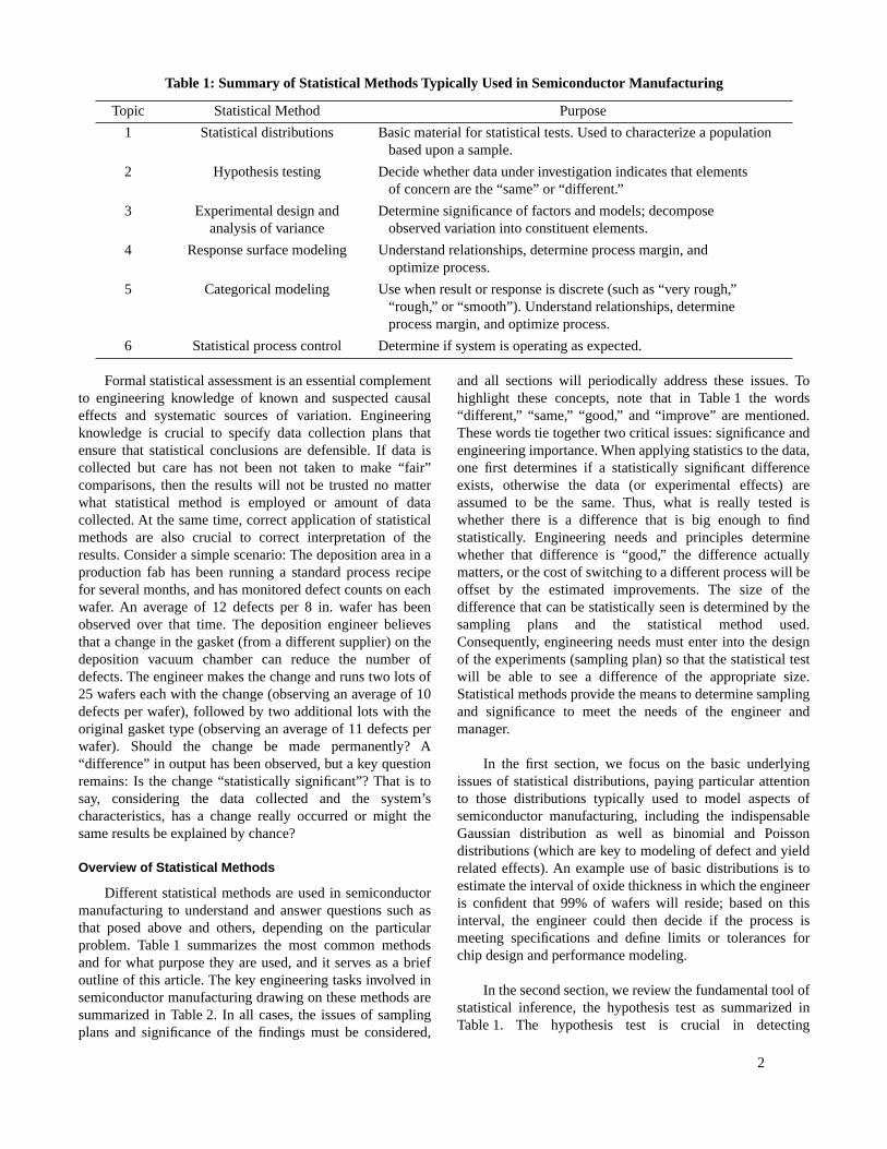
For example, if one is starting a 25-wafer lot in the fababove, one may wish to know what is the probability thatsome number x (x being between 0 and 25) of those waferswill survive. For the line yield model of p = 95%, theseprobabilities are shown in Fig. 1. When n is very large (muchlarger than 25), the binomial distribution is wellapproximated by a Gaussian distribution.

A key assumption in using the Bernoulli distribution isthat each wafer is independent of the other wafers in the lot.One often finds that many lots complete processing with allwafers intact, and other lots suffer multiple damaged wafers.While an aggregate line yield of 95% may result,independence does not hold and alternative approaches suchas formation of empirical distributions should be used.

Poisson Distribution. A third discrete distribution is highlyrelevant to semiconductor manufacturing. An approximationto the binomial distribution that applies when n is large and pis small is the Poisson distribution:

(9)

for integer and .

For example, one can examine the number of chips thatfail on the first day of operation: The probability p of failurefor any one chip is (hopefully) exceedingly small, but onetests a very large number n of chips, so that the observationof the mean number of failed chips is Poissondistributed. An even more common application of thePoisson model is in defect modeling. For example, if defects

are Poisson-distributed with a mean defect count of 3particles per 200 mm wafer, one can ask questions about theprobability of observing x [e.g., Eq. (9)] defects on a sample

wafer. In this case, , or lessthan 0.3% of the time would we expect to observe exactly 9defects. Similarly, the probability that 9 or more defects are

observed is .

In the case of defect modeling, several otherdistributions have historically been used, including theexponential, hypergeometric, modified Poisson, and negativebinomial. Substantial additional work has been reported inyield modeling to account for clustering, and to understandthe relationship between defect models and yield (e.g., seeRef. 4).

Population Versus Sample Statistics

We now have the beginnings of a statistical inference theory.Before proceeding with formal hypothesis testing in the nextsection, we first note that the earlier descriptive statistics ofmean and variance take on new interpretations in theprobabilistic framework. The mean is the expectation (or“first moment”) over the distribution:

(10)

for continuous pdf’s and discrete pmf’s, respectively.Similarly, the variance is the expectation of the squareddeviation from the mean (or the “second central moment”)over the distribution:

(11)

Further definitions from probability theory are also highlyuseful, including the covariance:

(12)

where x and y are each random variables with their ownprobability distributions, as well as the related correlationcoefficient:

(13)

The above definitions for the mean, variance,covariance, and correlation all relate to the underlying or

Figure 1. Probabilities for number of wafers survivingfrom a lot of 25 wafers, assuming a line yield of 90%,calculated using the binomial distribution.

f x p n, ,( ) nx

px

1 p–( )n x–=

nx

n!x! n x–( )!-----------------------=

0

0.05

0.1

0.15

0.2

0.25

0.3

0.35

0.4

0 5 1 0 1 5 2 0 2 5

Wafers surviving

f x λ,( ) eλ– λ x

x!--------------=

λ 0 1 2 …, , ,= λ np≅

λ np=

f 9 3,( ) e3–3

9( ) 9!⁄ 0.0027= =

1 f x 3,( )x 0=

8

∑– 0.0038=

µx E x{ } xf x( ) xd

∞–

∞

∫= =

xi p⋅r

xi( )i 1=

n

∑=

σx2

Var x{ } x E x{ }–( )2f x( ) xd

∞–

∞

∫= =

xi E xi{ }–( )2p⋅ r xi( )

i 1=

n

∑=

σxy2

Cov x y,{ } E x E x{ }–( ) y E y{ }–( ){ }= =

E xy{ } E x{ } E y{ }–=

ρxy Corr x y,{ } Cov x y,{ }Var x{ } Var y{ }

------------------------------------------σxy

2

σxσy------------= = =

6

assumed population. When one only has a sample (that is, afinite number of values drawn from some population), onecalculates the corresponding sample statistics. These are nolonger “descriptive” of only the sample we have; rather,these statistics are now estimates of parameters in aprobability model. Corresponding to the populationparameters above, the sample mean is given by Eq. (1), the

sample variance by Eq. (2), the sample std. dev. by Eq.

(3), the sample covariance is given by

(14)

and the sample correlation coefficient is given by

(15)

Sampling Distributions

Sampling is the act of making inferences about populationsbased on some number of observations. Random sampling isespecially important and desirable, where each observationis independent and identically distributed. A statistic is afunction of sample data which contains no further unknowns(e.g., the sample mean can be calculated from theobservations and has no further unknowns). It is important tonote that a sample statistic is itself a random variable and hasa “sampling distribution” which is usually different than theunderlying population distribution. In order to reason aboutthe “likelihood” of observing a particular statistic (e.g., themean of five measurements), one must be able to constructthe underlying sampling distribution.

Sampling distributions are also intimately bound upwith estimation of population distribution parameters. Forexample, suppose we know that the thickness of gate oxide(at the center of the wafer) is normally distributed:

. We sample five random wafers

and compute the mean oxide thickness

. We now have two key questions:

(1) What is the distribution of ? (2) What is the probability

that ?

In this case, given the expression for above, we can

use the fact that the variance of a scaled random variable

is simply , and the variance of a sum ofindependent random variables is the sum of the variances

(16)

where by the definition of the mean. Thus,

when we want to reason about the likelihood of observing

values of (that is, averages of five sample measurements)

lying within particular ranges, we must be sure to use the

distribution for rather than that for the underlyingdistribution T. Thus, in this case the probability of finding a

value between 105 Å and 120 Å is

(17)

which is relatively unlikely. Compare this to the result fromEq. (6) for the probability 0.0569 of observing a single value(rather than a five sample average) in the range 105 Å to 120Å.

Note that the same analysis would apply if was itself

formed as an average of underlying oxide thicknessmeasurements (e.g., from a nine point pattern across thewafer), if that average and each of the five

wafers used in calculating the sample average are

independent and also distributed as .

Chi-Square Distribution and Variance Estimates. Severalother vitally important distributions arise in sampling, andare essential to making statistical inferences in experimentaldesign or regression. The first of these is the chi-squaredistribution. If for and

, then y is distributed as chi-square with

n degrees of freedom, written as . While formulas for

the probability density function for exist, they are almostnever used directly and are again instead tabulated or

available via statistical packages. The typical use of the isfor finding the distribution of the variance when the mean isknown.

Suppose we know that . As discussed

previously, we know that the mean over our n observations is

distributed as . How is the sample variance over our n observations distributed? We note that each

is normally distributed; thus if we

normalize our sample variance by we have a chi-square distribution:

x

sx2

sx

sxy2 1

n 1–------------ xi x–( ) yi y–( )

i 1=

n

∑=

rxy

sxy

sxsy---------=

Ti N µ σ2,( )∼ N 100 10,( )=

T15--- T1 T2 … T5+ + +( )=

T

a T b≤ ≤

T

ax

a2Var x{ }

T N µ σ2n⁄,( )∼

µT

µT µ= =

T

T

T

Pr 105 T 120≤ ≤( )

Pr105 µ–

σ n( )⁄------------------- T µ–

σ n( )⁄------------------- 120 µ–

σ n( )⁄-------------------≤ ≤

=

Pr105 100–

10( ) 5( )⁄------------------------------- T µ–

σ n( )⁄------------------- 120 100–

2------------------------≤ ≤

=

Pr zl z zu≤ ≤( )=

Φ 14.142( ) Φ 3.536( )– 0.0002= =

Ti

Ti N 100 10,( )∼

T

N 100 10,( )

xi N 0 1,( )∼ i 1 2 … n, , ,=

y x12

x22 … xn

2+ + +=

y χn2∼

χ2

χ2

xi N µ σ2,( )∼

x N µ σ2n⁄,( )∼ s

2

xi x–( ) N 0 σ2,( )∼

s2 σ2

7

(18)

where one degree of freedom is used in calculation of .Thus, the sample variance for n observations drawn from

is distributed as chi-square as shown in Eq. (18).

For our oxide thickness example where

and we form sample averages as above, then

and 95% of the time the observed sample variable will be

less than 1.78 Å2. A control chart could thus be constructedto detect when unusually large five-wafer sample variancesoccur.

Student t Distribution. The Student t distribution is anotherimportant sampling distribution. The typical use is when wewant to find the distribution of the sample mean when thetrue standard deviation is not known. Consider

(19)

In the above, we have used the definition of the Student tdistribution: if is a random variable, , then

is distributed as a Student t with k degrees of

freedom, or , if . is a random variable

distributed as . As discussed previously, the normalized

sample variance is chi-square-distributed, so that ourdefinition does indeed apply. We thus find that thenormalized sample mean is distributed as a Student t with n-1 degrees of freedom when we do not know the true standarddeviation and must estimate it based on the sample as well.We note that as , the Student t approaches a unit

normal distribution .

F Distribution and Ratios of Variances. The last samplingdistribution we wish to discuss here is the F distribution. Weshall see that the F distribution is crucial in analysis ofvariance (ANOVA) and experimental design in determiningthe significance of effects, because the F distribution isconcerned with the probability density function for the ratio

of variances. If (that is, is a random variable

distributed as chi-square with u degrees of freedom) and

similarly , then the random variable

(that is, distributed as F with u and v degrees of freedom).The typical use of the F distribution is to compare the spreadof two distributions. For example, suppose that we have twosamples and , where

and . Then

(20)

Point and Interval Estimation

The above population and sampling distributions formthe basis for the statistical inferences we wish to draw inmany semiconductor manufacturing examples. Oneimportant use of the sampling distributions is to estimatepopulation parameters based on some number ofobservations. A point estimate gives a single “best”estimated value for a population parameter. For example, the

sample mean is an estimate for the population mean .Good point estimates are representative or unbiased (that is,the expected value of the estimate should be the true value),as well as minimum variance (that is, we desire the estimatorwith the smallest variance in that estimate). Often we restrictourselves to linear estimators; for example, the best linearunbiased estimator (BLUE) for various parameters istypically used.

Many times we would like to determine a confidenceinterval for estimates of population parameters; that is, wewant to know how likely it is that is within some particular

range of . Asked another way, to a desired probability,

where will actually lie given an estimate ? Such intervalestimation is considered next; these intervals are used in latersections to discuss hypothesis testing.

First, let us consider the confidence interval forestimation of the mean, when we know the true variance ofthe process. Given that we make n independent andidentically distributed samples from the population, we cancalculate the sample mean as in Eq. (1). As discussed earlier,we know that the sample mean is normally distributed asshown in Eq. (16). We can thus determine the probability

that an observed is larger than by a given amount:

(21)

where is the alpha percentage point for the normalized

variable z (that is, measures how many standard

deviations greater than we must be in order for the

s2

xi x–( )2

i∑

n 1–( )⁄=

n 1–( )s2

σ2---------------------- χn 1–

2∼

s2 σ2

n 1–( )---------------- χ⋅

n 1–

2

∼

x

N µ σ2,( )

Ti N 100 10,( )∼

T sT

210χ4

24⁄∼

σ

xi N µ σ2,( )∼

x µ–

s n( )⁄------------------

x µ–

σ n( )⁄-------------------

s σ⁄------------------------- N 0 1,( )

1n 1–------------χn 1–

2----------------------------- tn 1–∼ ∼=

z z N 0 1,( )∼

z y k⁄( )⁄

z y k⁄( )⁄ tk∼ y

χk2

s2 σ2⁄

k ∞→tk N 0 1,( )→

y1 χu2∼ y1

y2 χv2∼ Y

y1 u⁄y2 v⁄------------ Fu v,∼=

x1 x2 … xn, , , w1 w2 … wm, , ,

xi N µx σx2,( )∼ wi N µw σw

2,( )∼

sx2 σx

2⁄

sw2 σw

2⁄---------------- Fn 1– m 1–,∼

x µ

x

µµ x

x µ

zx µ–

σ n( )⁄-------------------=

Pr z zα>( ) α 1 Φ zα( )–= =

zα

zα

µ

8

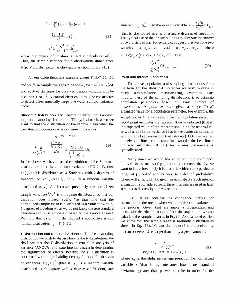
integrated probability density to the right of this value toequal ). As shown in Fig. 2, we are usually interested inasking the question the other way around: to a givenprobability [ , e.g., 95%], in what range will the

true mean lie given an observed ?

(22)

.

For our oxide thickness example, we can now answer animportant question. If we calculate a five-wafer average, howfar away from the average 100 Å must the value be for us todecide that the process has changed away from the mean

(given a process variance of 10 Å2)? In this case, we mustdefine the “confidence” in saying that the process haschanged; this is equivalent to the probability of observing thedeviation by chance. With 95% confidence, we can declarethat the process is different than the mean of 100 Å if we

observe Å or Å:

(23)

A similar result occurs when the true variance is notknown. The confidence interval in this case isdetermined using the appropriate Student t samplingdistribution for the sample mean:

(24)

In some cases, we may also desire a confidence intervalon the estimate of variance:

(25)

For example, consider a new etch process which wewant to characterize. We calculate the average etch rate(based on 21-point spatial pre- and post-thicknessmeasurements across the wafer) for each of four wafers weprocess. The wafer averages are 502, 511, 515, and 504 Å/min. The sample mean is Å/min, and the sample

standard deviation is Å/min. The 95% confidence

intervals for the true mean and std. dev. are

Å/min, and Å/min. Increasing the number ofobservations (wafers) can improve our estimates andintervals for the mean and variance, as discussed in the nextsection.

Many other cases (e.g., one-sided confidence intervals)can also be determined based on manipulation of theappropriate sampling distributions, or through consultationwith more extensive texts (5).

HYPOTHESIS TESTING

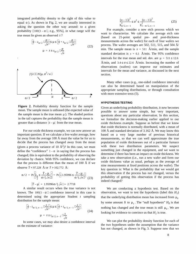
Given an underlying probability distribution, it now becomespossible to answer some simple, but very important,questions about any particular observation. In this section,we formalize the decision-making earlier applied to ouroxide thickness example. Suppose as before that we knowthat oxide thickness is normally distributed, with a mean of100 Å and standard deviation of 3.162 Å. We may know thisbased on a very large number of previous historicalmeasurements, so that we can well approximate the truepopulation of oxide thicknesses out of a particular furnacewith these two distribution parameters. We suspectsomething just changed in the equipment, and we want todetermine if there has been an impact on oxide thickness. Wetake a new observation (i.e., run a new wafer and form ouroxide thickness value as usual, perhaps as the average ofnine measurements at fixed positions across the wafer). Thekey question is: What is the probability that we would getthis observation if the process has not changed, versus theprobability of getting this observation if the process hasindeed changed?

We are conducting a hypothesis test. Based on theobservation, we want to test the hypothesis (label this H1)

that the underlying distribution mean has increased from

by some amount to . The “null hypothesis” H0 is that

nothing has changed and the true mean is still . We are

looking for evidence to convince us that H1 is true.

We can plot the probability density function for each ofthe two hypotheses under the assumption that the variancehas not changed, as shown in Fig. 3. Suppose now that we

Figure 2. Probability density function for the samplemean. The sample mean is unbiased (the expected value ofthe sample mean is the true mean ). The shaded portionin the tail captures the probability that the sample mean isgreater than a distance from the true mean.

α

100 1 α–( )x

x zα 2⁄σn

-------⋅– µ x zα 2⁄+

σn

-------⋅ ≤ ≤

µ x zα 2⁄σn

-------⋅±=

x

f x( ) N µ σ2n⁄,( )∼

µ α 2⁄α 2⁄ x

µ

x µ–

1 α–

T 97.228< T 102.772>

α 2⁄ Pr zα2---

T µ–

σ n( )⁄-------------------≤

Pr 1.95996–T µ–

σ n( )⁄-------------------≤

= =

T µ– 1.95996σ n( )⁄ 2.7718= =

100 1 α–( )

x tα 2⁄ n 1–,s

n-------⋅–

µ x tα 2⁄ n 1–,+s

n-------⋅

≤ ≤

µ x tα 2⁄ n 1–,s

n-------⋅±=

n 1–( )s2

χα 2⁄ n 1–,2

----------------------- σ2 n 1–( )s2

χ1 α 2⁄– n 1–,2

------------------------------≤ ≤

x 511=

s 6.1=

µ 511 12.6±=

3.4 σ 22.6≤ ≤

µ0

δ µ1

µ0

9

observe the value . Intuitively, if the value of is “closer”

to than to , we will more than likely believe that the

value comes from the H0 distribution than the H1

distribution. Under a maximum likelihood approach, we cancompare the probability density functions:

(26)

that is, if is greater than for our observation, we reject

the null hypothesis H0 (that is, we “accept” the alternativehypothesis H1). If we have prior belief (or other knowledge)affecting the a priori probabilities of H0 and H1, these can

also be used to scale the distributions and to

determine a posterior probabilities for H0 and H1. Similarly,we can define the “acceptance region” as the set of values of

for which we accept each respective hypothesis. In Fig. 3,

we have the rule: accept H1 if , and accept H0 if

.

The maximum likelihood approach provides a powerfulbut somewhat complicated means for testing hypotheses. Intypical situations, a simpler approach suffices. We select aconfidence with which we must detect a “difference,”

and we pick a decision point based on that confidence.For two-sided detection with a unit normal distribution, forexample, we select and as the regions for

declaring that unusual behavior (i.e., a shift) has occurred.

Consider our historical data on oxide thickness where. To be 95% confident that a new observation

indicates a change in mean, we must observe Å or

Å. On the other hand, if we form five-wafer

averages, then we must observe Å or Å asin Eq. (23) to convince us (to 95% confidence) that ourprocess has changed.

Alpha and Beta Risk (Type I and Type II Errors)

The hypothesis test gives a clear, unambiguous procedure formaking a decision based on the distributions andassumptions outlined above. Unfortunately, there may be asubstantial probability of making the wrong decision. In themaximum likelihood example of Fig. 3, for the singleobservation as drawn we accept the alternative hypothesis

H1. However, examining the distribution corresponding to

H0, we see that a nonzero probability exists of belonging

to H1.Two types of errors are of concern:

(27)

We note that the Type I error (or probability of a“false alarm”) is based entirely on our decision rule and doesnot depend on the size of the shift we are seeking to detect.The Type II error (or probability of “missing” a real shift),on the other hand, depends strongly on the size of the shift.This Type II error can be evaluated for the distributions anddecision rules above; for the normal distribution of Fig. 3,we find

(28)

where is the shift we wish to detect.

The “power” of a statistical test is defined as

(29)

that is, the power of the test is the probability of correctlyrejecting H0. Thus the power depends on the shift we wish

to detect as well as the level of “false alarms” ( or Type Ierror) we are willing to endure. Power curves are oftenplotted of versus the normalized shift to detect ,

for a given fixed (e.g., ), and as a function ofsampling size.

Hypothesis Testing and Sampling Plans. In the previousdiscussion, we described a hypothesis test for detection of ashift in mean of a normal distribution, based on a singleobservation. In realistic situations, we can often makemultiple observations and improve our ability to make acorrect decision. If we take n observations, then the sample

Figure 3. Distributions of x under the null hypothesis H0,and under the hypothesis H1 that a positive shift has

occurred such that .

xi xi

µ0 µ1

f 0 xi( )H0><H1

f 1 xi( )

f 1 f 0

f 0 f 1

xi

xi x*>

xi x*<

x

H0: f 0 x( ) N µ0 σ2,( )∼

µ1µ0 δ

xix*

µ1 µ0 δ+=

1 α–

x*

z zα 2⁄> z zα 2⁄–<

Ti N 100 10,( )∼

Ti 93.8<

Ti 106.2>

T 97.2< T 102.8>

xi

xi

α Pr (Type I error)=

Pr reject H0 H0 is true( ) f 0 x( ) xd

x*

∞

∫= =

β Pr (Type II error)=

Pr accept H0 H1 is true( ) f 1 x( ) xd

∞–

x*

∫= =

α

β

β Φ zα 2⁄δσ---–

Φ zα 2⁄– δσ---–

–=

δ

Power 1 β–≡ Pr reject H0 H0 is false( )=

δ

α

β d δ σ⁄=

α α 0.05=

10

mean is normally distributed, but with a reduced variance

as illustrated by our five-wafer average of oxide

thickness. It now becomes possible to pick an riskassociated with a decision on the sampling distribution thatis acceptable, and then determine a sample size n in order toachieve the desired level of risk. In the first step, we still

select based on the risk of false alarm , but now this

determines the actual unnormalized decision point using

. We finally pick n (which determines

as just defined) based on the Type II error, which also

depends on the size of the normalized shift to bedetected and the sample size n. Graphs and tables areindispensable in selecting the sample size for a given d and

; for example, Fig. 4 shows the Type II error associatedwith sampling from a unit normal distribution, for a fixedType I error of 0.05, and as a function of sampling size n andshift to be detected d.

Consider once more our wafer average oxide thickness

. Suppose that we want to detect a 1.58 Å (or 0.5 ) shift

from the 100 Å mean. We are willing to accept a false alarm5% of the time ( ) but can accept missing the shift

20% of the time ( ). From Fig. 4, we need to take

. Our decision rule is to declare that a shift has

occurred if our 30 sample average Å or Å.

If it is even more important to detect the 0.5 shift in mean

(e.g., with probability of missing the shift), then

from Fig. 4 we now need samples, and our decision

rule is to declare a shift if the 40 sample average Å

or Å.

Control Chart Application. The concepts of hypothesistesting, together with issues of Type I and Type II error aswell as sample size determination, have one of their mostcommon applications in the design and use of control charts.

For example, the control chart can be used to detect whena “significant” change from “normal” operation occurs. Theassumption here is that when the underlying process isoperating under control, the fundamental process population

is distributed normally as . We periodically

draw a sample of n observations and calculate the average ofthose observations ( ). In the control chart, we essentiallyperform a continuous hypothesis test, where we set the upperand lower control limits (UCLs and LCLs) such that falls

outside these control charts with probability when the

process is truly under control (e.g., we usually select togive a 0.27% chance of false alarm). We would then choosethe sample size n so as to have a particular power (that is, aprobability of actually detecting a shift of a given size) aspreviously described. The control limits (CLs) would then beset at

(30)

Note that care must be taken to check key assumptionsin setting sample sizes and control limits. In particular, oneshould verify that each of the n observations to be utilized informing the sample average (or the sample standarddeviation in an s chart) are independent and identicallydistributed. If, for example, we aggregate or take the averageof n successive wafers, we must be sure that there are nosystematic within-lot sources of variation. If such additionalvariation sources do exist, then the estimate of varianceformed during process characterization (e.g., in our etchexample) will be inflated by accidental inclusion of thissystematic contribution, and any control limits one sets willbe wider than appropriate to detect real changes in theunderlying random distribution. If systematic variation doesindeed exist, then a new statistic should be formed thatblocks against that variation (e.g., by specifying whichwafers should be measured out of each lot), and the controlchart based on the distribution of that aggregate statistic.

EXPERIMENTAL DESIGN AND ANOVA

In this section, we consider application and furtherdevelopment of the basic statistical methods alreadydiscussed to the problem of designing experiments toinvestigate particular effects, and to aid in the construction ofmodels for use in process understanding and optimization.First, we should recognize that the hypothesis testingmethods are precisely those needed to determine if a newtreatment induces a significant effect in comparison to aprocess with a known distribution. These are known as one-sample tests. In this section, we next consider two-sample

Figure 4. Probability of Type II error ( ) for a unit

normal process with Type I error fixed at , as afunction of sample size n and shift delta (equal to thenormalized shift ) to be detected.

σ2n⁄

α

βzα 2⁄ α

x* µ z+ α 2⁄ σ n( )⁄⋅=

x*

d δ σ⁄=

α

0

0.1

0.2

0.3

0.4

0.5

0.6

0.7

0.8

0.9

1

0 0.5 1 1.5 2

Delta (in units of standard deviation)

n = 2

n = 3

n = 5

n = 10n = 20

n = 30

n = 40

βα 0.05=

δ σ⁄

Ti σ

α 0.05=

β 0.20=

n 30=

T 98.9< T 101.1>σ

β 0.10=

n 40=

T 99.0<

T 101.0>

x

xi N µ σ2,( )∼

x

x

α3σ

CL µ zα 2⁄σn

-------⋅ ±=

11

tests to compare two treatments in an effort to detect atreatment effect. We will then extend to the analysis ofexperiments in which many treatments are to be compared(k-sample tests), and we present the classic tool for studyingthe results --- ANOVA (6).

Comparison of Treatments: Two-Sample Tests

Consider an example where a new process B is to becompared against the process of record (POR), process A. Inthe simplest case, we have enough historical information onprocess A that we assume values for the yield mean and

standard deviation . If we gather a sample of 10 wafers forthe new process, we can perform a simple one-samplehypothesis test using the 10 wafer sampling

distribution and methods already discussed, assuming thatboth process A and B share the same variance.

Consider now the situation where we want to comparetwo new processes. We will fabricate 10 wafers with processA and another 10 wafers with process B, and then we willmeasure the yield for each wafer after processing. In order toblock against possible time trends, we alternate betweenprocess A and process B on a wafer by wafer basis. We areseeking to test the hypothesis that process B is better thanprocess A, that is H1: , as opposed to the null

hypothesis H0: . Several approaches can be used

(5).

In the first approach, we assume that in each process Aand B we are random sampling from an underlying normaldistribution, with (1) an unknown mean for each process and(2) a constant known value for the population standard

deviation of . Then , ,

, and . We can then

construct the sampling distribution for the difference inmeans as

(31)

(32)

Even if the original process is moderately non-normal, thedistribution of the difference in sample means will beapproximately normal by the central limit theorem, so wecan normalize as

(33)

allowing us to examine the probability of observing themean difference based on the unit normal

distribution, .

The disadvantage of the above method is that it dependson knowing the population standard deviation . If suchinformation is indeed available, using it will certainlyimprove the ability to detect a difference. In the secondapproach, we assume that our 10 wafer samples are againdrawn by random sampling on an underlying normalpopulation, but in this case we do not assume that we know apriori what the population variance is. In this case, we mustalso build an internal estimate of the variance. First, we

estimate from the individual variances:

(34)

and similarly for . The pooled variance is then

(35)

Once we have an estimate for the population variance, wecan perform our t test using this pooled estimate:

(36)

One must be careful in assuming that process A and B sharea common variance; in many cases this is not true and moresophisticated analysis is needed (5).

Comparing Several Treatment Means via ANOVA

In many cases, we are interested in comparing severaltreatments simultaneously. We can generalize the approachdiscussed above to examine if the observed differences intreatment means are indeed significant, or could haveoccurred by chance (through random sampling of the sameunderlying population).

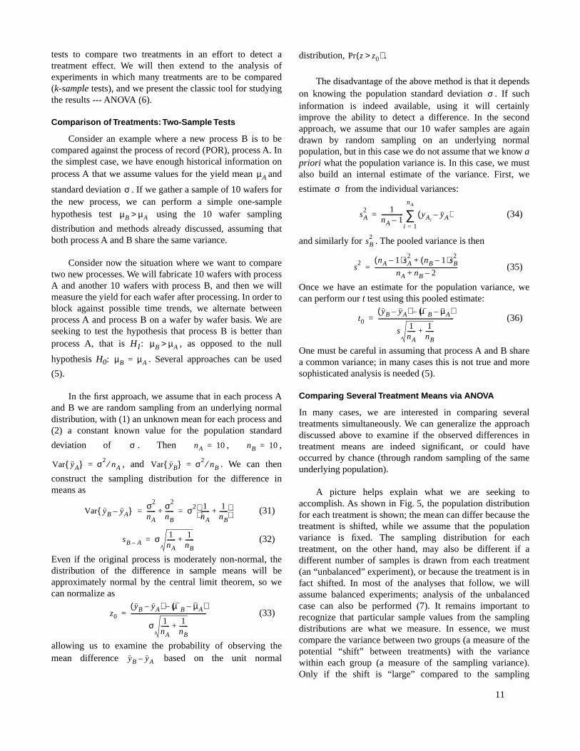
A picture helps explain what we are seeking toaccomplish. As shown in Fig. 5, the population distributionfor each treatment is shown; the mean can differ because thetreatment is shifted, while we assume that the populationvariance is fixed. The sampling distribution for eachtreatment, on the other hand, may also be different if adifferent number of samples is drawn from each treatment(an “unbalanced” experiment), or because the treatment is infact shifted. In most of the analyses that follow, we willassume balanced experiments; analysis of the unbalancedcase can also be performed (7). It remains important torecognize that particular sample values from the samplingdistributions are what we measure. In essence, we mustcompare the variance between two groups (a measure of thepotential “shift” between treatments) with the variancewithin each group (a measure of the sampling variance).Only if the shift is “large” compared to the sampling

µA

σ

µB µA>

µB µA>

µB µA=

σ nA 10= nB 10=

Var yA{ } σ 2nA⁄= Var yB{ } σ 2

nB⁄=

Var yB yA–{ } σ2

nA------ σ2

nB------+ σ2 1

nA------ 1

nB------+

= =

sB A– σ 1nA------ 1

nB------+=

z0

yB yA–( ) µB µA–( )–

σ 1nA------ 1

nB------+

-----------------------------------------------------=

yB yA–

Pr z z0>( )

σ

σ

sA2 1

nA 1–--------------- yAi

yA–( )i 1=

nA

∑=

sB2

s2 nA 1–( )sA

2nB 1–( )sB

2+

nA nB 2–+----------------------------------------------------------=

t0

yB yA–( ) µB µA–( )–

s1

nA------ 1

nB------+

-----------------------------------------------------=

12

variance are we confident that a true effect is in place. Anappropriate sample size must therefore be chosen usingmethods previously described such that the experiment ispowerful enough to detect differences between thetreatments that are of engineering importance. In thefollowing, we discuss the basic methods used to analyze theresults of such an experiment (8).

First, we need an estimate of the within-group variation.Here we again assume that each group is normally

distributed and share a common variance . Then we can

form the “sum of squares” deviations within the tth group as

(37)

where is the number of observations or samples in group

t. The estimate of the sample variance for each group, alsoreferred to as the “mean square,” is thus

(38)

where is the degrees of freedom in treatment t. We can

generalize the pooling procedure used earlier to estimate acommon shared variance across k treatments as

(39)

where is defined as the within-treatment or within-

group mean square and is the total number of

measurements, , or simply if

all treatments consist of the same number of samples, .

In the second step, we want an estimate of between-group variation. We will ultimately be testing the hypothesis

. The estimate of the between-group

variance is

(40)

where is defined as the between treatment mean

square, , and is the overall mean.

We are now in position to ask our key question: Are thetreatments different? If they are indeed different, then thebetween-group variance will be larger than the within-groupvariance. If the treatments are the same, then the between-group variance should be the same as the within-groupvariance. If in fact the treatments are different, we thus findthat

(41)

where is treatment t’s effect. That is, is

inflated by some factor related to the difference betweentreatments. We can perform a formal statistical test fortreatment significance. Specifically, we should consider theevidence to be strong for the treatments being different if the

ratio is significantly larger than 1. Under our

assumptions, this should be evaluated using the F

distribution, since .

We can also express the total variation (total deviationsum of squares from the grand mean ) observed in the

data as

(42)

where is recognized as the variance in the data.

Analysis of variance results are usually expressed intabular form, such as shown in Table 3. In addition tocompactly summarizing the sum of squares due to variouscomponents and the degrees of freedom, the appropriate Fratio is shown. The last column of the table usually containsthe probability of observing the stated F ratio under the nullhypothesis. The alternative hypothesis --- that one or more

Figure 5. Pictorial representation of multiple treatmentexperimental analysis. The underlying population for eachtreatment may be different, while the variance for eachtreatment population is assumed to be constant. The darkcircles indicate the sample values drawn from thesepopulations (note that the number of samples may not bethe same in each treatment).

A B C

y

yA

yB

yC

Populationdistributions

σ2

SSt

SSt yt jyt–( )

2

j 1=

nt

∑=

nt

st2 SSt

υ t-------

SSt

nt 1–-------------= =

υ t

sR2 υ1s1

2 υ2s22 … υksk

2+ + +

υ1 υ2 … υk+ + +----------------------------------------------------------

SSR

N k–-------------

SSR

υR---------= = =

SSR υR⁄

N

N n1 n2 … nk+ + += N nk=

k n

µ1 µ2 … µk= = =

sT2

nt yt y–( )2

t 1=

k

∑SST

υT---------= =

SST υT⁄

υT k 1–= y

sT2

estimates σ2 ntτ t2

k 1–( )----------------

t 1=

k

∑+

τ t µt µ–= sT2

sT2

sR2⁄

sT2

sR2⁄ Fk 1– N k–,∼

SSD

SSD yti y–2( )

i 1=

nt

∑t 1=

k

∑=

sD2 SSD

υD----------

SSD

N 1–-------------= =

sD2

13

treatments have a mean different than the others --- can beaccepted with confidence.

As summarized in Table 3, analysis of variance can alsobe pictured as a decomposition of the variance observed inthe data. That is, we can express the total sum of squareddeviations from the grand mean as , or the

between-group sum of squares added to the within-groupsum of squares. We have presented the results here aroundthe grand mean. In some cases, an alternative presentation is

used where a “total” sum of squares

is used. In this case the total sum of squares also includes

variation due to the average, , or

. In Table 3, k is the

number of treatments and N is the total number of

observations. The F ratio value is , which is compared

against the F ratio for the degrees of freedom and .

The p value shown in such a table is

Pr( ).

While often not explicitly stated, the above ANOVAassumes a mathematical model:

(43)

where are the treatment means, and are the residuals:

(44)

where is the estimated treatment mean. It is

critical that one check the resulting ANOVA model. First, theresiduals should be plotted against the time order in

which the experiments were performed in an attempt todistinguish any time trends. While it is possible to randomizeagainst such trends, we lose resolving power if the trend islarge. Second, one should examine the distribution of theresiduals. This is to check the assumption that the residualsare “random” [that is, independent and identically distributed(IID) and normally distributed with zero mean] and look forgross non-normality. This check should also include anexamination of the residuals for each treatment group. Third,one should plot the residuals versus the estimates and be

especially alert to dependencies on the size of the estimate(e.g., proportional versus absolute errors). Finally, oneshould also plot the residuals against any other variables ofinterest, such as environmental factors that may have beenrecorded. If unusual behavior is noted in any of these steps,additional measures should be taken to stabilize the variance(e.g., by considering transformations of the variables or byreexamining the experiment for other factors that may needto be either blocked against or otherwise included in theexperiment).

Two-Way Analysis of Variance

Suppose we are seeking to determine if various treatmentsare important in determining an output effect, but we mustconduct our experiment in such a way that another variable(which may also impact the output) must also vary. Forexample, suppose we want to study two treatments A and Bbut must conduct the experiments on five different processtools (tools 1-5). In this case, we must carefully design theexperiment to block against the influence of the process toolfactor. We now have an assumed model:

(45)

where are the block effects. The total sum of squares

can now be decomposed as(46)

with degrees of freedom(47)

where b is the number of blocking groups, k is the

number of treatment groups, and . As

before, if the blocks or treatments do in fact include anymean shifts, then the corresponding mean sum of squares(estimates of the corresponding variances) will again beinflated beyond the population variance (assuming thenumber of samples at each treatment is equal):

(48)

Table 3: Structure of the Analysis of Variance Table, for Single Factor (Treatment) Case

Source of Variation Sum of Squares Degrees of Freedom Mean Square

F ratio Pr(F)

Between treatments

Within treatments

Total about the grand mean

SST υT k 1–= sT2

sT2

sR2⁄ p

SSR υR N k–= sR2

SSD SST SSR+= υD υT υR+ N 1–= = sD2

100 1 p–( )

SSD SST SSR+=

SS y12

y22 … yN

2+ + +=

SSA Ny2

=

SS SSA SSD+ SSA SST SSR++= =

sT2

sR2⁄

υT υR

FυT υR, sT2

sR2⁄> µ1 … µk= =

yti µt εti+ µ τ t εti+ += =

µt εti

εti yti ytiˆ– N 0 σ2,( )∼=

ytiˆ yt

ˆ µ τ t+= =

εti

yti µ τ t β+ +i

εti+=

βi SS

SS SSA SSB+ SST SSR+ +=

bk 1 b 1–( ) k 1–( ) b 1–( ) k 1–( )+ + +=

SSB k yi y–( )2

i 1=

b

∑=

sB2

estimates σ2k

βi2

b 1–( )----------------

i 1=

b

∑+

sT2

estimates σ2 ntτ t2

k 1–( )----------------

t 1=

k

∑+

14

where we assume that k samples are observed for each of theb blocks. So again, we can now test the significance of thesepotentially “inflated” variances against the pooled estimate

of the variance with the appropriate F test as summarized

in Table 4. Note that in Table 4 we have shown the ANOVAtable in the non-mean centered or “uncorrected” format, sothat due to the average is shown. The table can be

converted to the mean corrected form as in Table 3 byremoving the row, and replacing the total with the

mean corrected total with degrees of

freedom.

Two-Way Factorial Designs

While the above is expressed with the terminology of thesecond factor being considered a “blocking” factor, preciselythe same analysis pertains if two factors are simultaneouslyconsidered in the experiment. In this case, the blockinggroups are the different levels of one factor, and thetreatment groups are the levels of the other factor. Theassumed analysis of variance above is with the simpleadditive model (that is, assuming that there are nointeractions between the blocks and treatments, or betweenthe two factors). In the blocked experiment, the intent of theblocking factor was to isolate a known (or suspected) sourceof “contamination” in the data, so that the precision of theexperiment can be improved.

We can remove two of these assumptions in ourexperiment if we so desire. First, we can treat both variablesas equally legitimate factors whose effects we wish toidentify or explore. Second, we can explicitly design theexperiment and perform the analysis to investigateinteractions between the two factors. In this case, the modelbecomes

(49)

where is the effect that depends on both factors

simultaneously. The output can also be expressed as

(50)

where is the overall grand mean, and are the main

effects, and are the interaction effects. In this case, the

subscripts are

The resulting ANOVA table will be familiar; the one keyaddition is explicit consideration of the interaction sum ofsquares and mean square. The variance captured in thiscomponent can be compared to the within-group variance asbefore, and be used as a measure of significance for theinteractions, as shown in Table 5.

Another metric often used to assess “goodness of fit” of

a model is the R2. The fundamental question answered by R2

is how much better does the model do than simply using thegrand average.

(51)

where is the variance or sum of square deviations

around the grand average, and is the variance captured

by the model consisting of experimental factors ( and

) and interactions ( ). An R2 value near zero indicates

that most of the variance is explained by residuals( ) rather than by the model terms ( ),

while an R2 value near 1 indicates that the model sum ofsquare terms capture nearly all of the observed variation in

Table 4: Structure of the Analysis of Variance Table,for the Case of a Treatment with a Blocking Factor

Source of Variation Sum of Squares Degrees of Freedom Mean Square

F ratio Pr(F)

Average (correction factor) 1

Between blocks

Between treatments

Residuals

Total

SSA nky2

=

SSB k yi y–( )2

i 1=

b

∑=υB b 1–= sB

2sB

2sR

2⁄ pB

SST b yt y–( )2

t 1=

k

∑=υT k 1–= sT

2sT

2sR

2⁄ pT

SSR υR b 1–( ) k 1–( )= sR2

SS υ N bk= = sD2

sR2

SSA

SSA SS

SSD υ N 1–=

ytij µti εtij+=

µti

µti µ τ t βi ωti+ + +=

y yt y–( ) yi y–( ) yti yt– yi– y+( )+ + +=

µ τ t βi

ωti

t 1 2 … k, , ,= where k is the # levels of first factor

i 1 2 … b, , ,= where b is the # levels of second factor

j 1 2 … m, , ,= where m is the # replicates at t, i factor

R2 SSM

SSD----------

SST SSB SSI+ +( )SSD

---------------------------------------------= =

SSD

SSM

SST

SSB SSI

SSR SSD SSM–= SSM

15

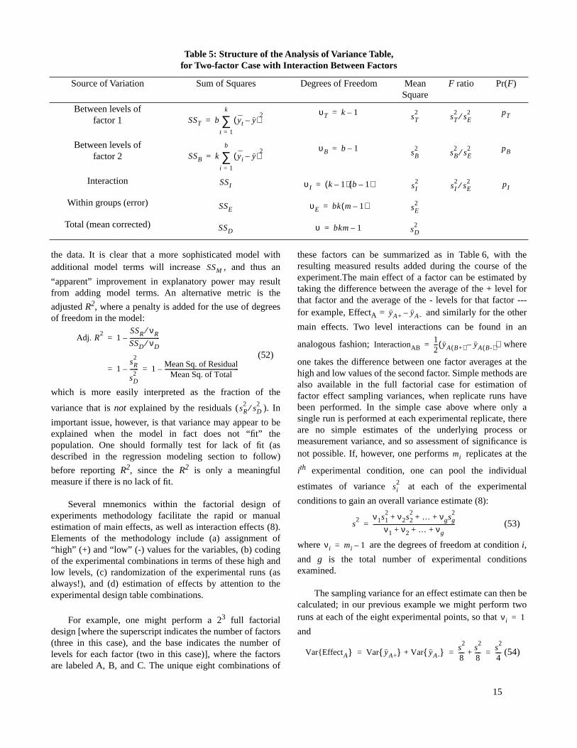
the data. It is clear that a more sophisticated model withadditional model terms will increase , and thus an

“apparent” improvement in explanatory power may resultfrom adding model terms. An alternative metric is the

adjusted R2, where a penalty is added for the use of degreesof freedom in the model:

(52)

which is more easily interpreted as the fraction of the

variance that is not explained by the residuals ( ). In

important issue, however, is that variance may appear to beexplained when the model in fact does not “fit” thepopulation. One should formally test for lack of fit (asdescribed in the regression modeling section to follow)

before reporting R2, since the R2 is only a meaningfulmeasure if there is no lack of fit.

Several mnemonics within the factorial design ofexperiments methodology facilitate the rapid or manualestimation of main effects, as well as interaction effects (8).Elements of the methodology include (a) assignment of“high” (+) and “low” (-) values for the variables, (b) codingof the experimental combinations in terms of these high andlow levels, (c) randomization of the experimental runs (asalways!), and (d) estimation of effects by attention to theexperimental design table combinations.

For example, one might perform a 23 full factorialdesign [where the superscript indicates the number of factors(three in this case), and the base indicates the number oflevels for each factor (two in this case)], where the factorsare labeled A, B, and C. The unique eight combinations of

these factors can be summarized as in Table 6, with theresulting measured results added during the course of theexperiment.The main effect of a factor can be estimated bytaking the difference between the average of the + level forthat factor and the average of the - levels for that factor ---for example, EffectA = and similarly for the other

main effects. Two level interactions can be found in an

analogous fashion; where

one takes the difference between one factor averages at thehigh and low values of the second factor. Simple methods arealso available in the full factorial case for estimation offactor effect sampling variances, when replicate runs havebeen performed. In the simple case above where only asingle run is performed at each experimental replicate, thereare no simple estimates of the underlying process ormeasurement variance, and so assessment of significance isnot possible. If, however, one performs replicates at the

ith experimental condition, one can pool the individual

estimates of variance at each of the experimental

conditions to gain an overall variance estimate (8):

(53)

where are the degrees of freedom at condition i,

and g is the total number of experimental conditionsexamined.

The sampling variance for an effect estimate can then becalculated; in our previous example we might perform tworuns at each of the eight experimental points, so that

and

(54)

Table 5: Structure of the Analysis of Variance Table, for Two-factor Case with Interaction Between Factors

Source of Variation Sum of Squares Degrees of Freedom Mean Square

F ratio Pr(F)

Between levels offactor 1

Between levels offactor 2

Interaction

Within groups (error)

Total (mean corrected)

SST b yt y–( )2

t 1=

k

∑=υT k 1–= sT

2sT

2sE

2⁄ pT

SSB k yi y–( )2

i 1=

b

∑=υB b 1–= sB

2sB

2sE

2⁄ pB

SSI υ I k 1–( ) b 1–( )= sI2

sI2

sE2⁄ pI

SSE υE bk m 1–( )= sE2

SSD υ bkm 1–= sD2

SSM

Adj. R2

1SSR νR⁄SSD νD⁄---------------------–=

1sR

2

sD2

------– 1 Mean Sq. of ResidualMean Sq. of Total

----------------------------------------------------–= =

sR2

sD2⁄

yA+ yA-–

InteractionAB12--- yA B+( ) yA B-( )–( )=

mi

si2

s2 ν1s1

2 ν2s22 … νgsg

2+ + +

ν1 ν2 … νg+ + +----------------------------------------------------------=

νi mi 1–=

νi 1=

Var{EffectA } Var yA+{ } Var yA-{ }+ s2

8---- s

2

8----+ s

2

4----= = =

16

These methods can be helpful for rapid estimation ofexperimental results and for building intuition aboutcontrasts in experimental designs; however, statisticalpackages provide the added benefit of assisting not only inquantifying factor effects and interactions, but also inexamination of the significance of these effects and creationof confidence intervals on estimation of factor effects andinteractions. Qualitative tools for examining effects includepareto charts to compare and identify the most importanteffects, and normal or half-normal probability plots todetermine which effects are significant.

In the discussion so far, the experimental factor levels aretreated as either nominal or continuous parameters. Animportant issue is the estimation of the effect of a particularfactor, and determination of the significance of any observedeffect. Such results are often pictured graphically in asuccinct fashion, as illustrated in Fig. 6 for a two-factorexperiment, where two levels for each of factor A and factorB are examined.

In the full factorial case, interactions can also beexplored, and the effects plots modified to show the effect of

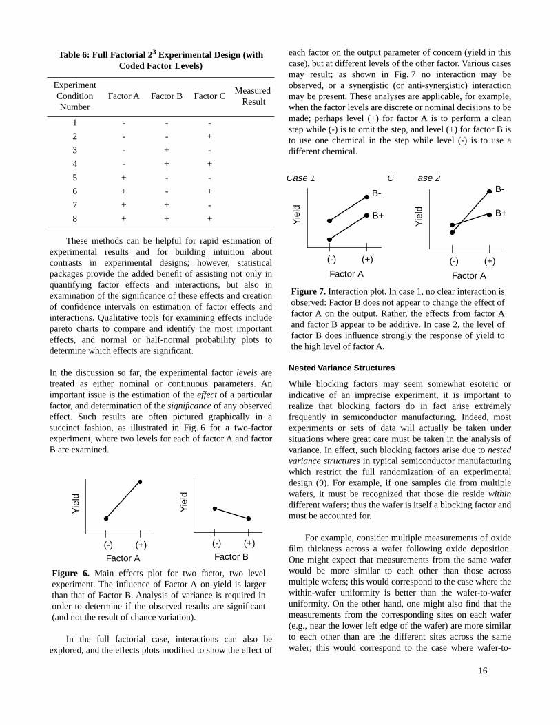
each factor on the output parameter of concern (yield in thiscase), but at different levels of the other factor. Various casesmay result; as shown in Fig. 7 no interaction may beobserved, or a synergistic (or anti-synergistic) interactionmay be present. These analyses are applicable, for example,when the factor levels are discrete or nominal decisions to bemade; perhaps level (+) for factor A is to perform a cleanstep while (-) is to omit the step, and level (+) for factor B isto use one chemical in the step while level (-) is to use adifferent chemical.

Nested Variance Structures

While blocking factors may seem somewhat esoteric orindicative of an imprecise experiment, it is important torealize that blocking factors do in fact arise extremelyfrequently in semiconductor manufacturing. Indeed, mostexperiments or sets of data will actually be taken undersituations where great care must be taken in the analysis ofvariance. In effect, such blocking factors arise due to nestedvariance structures in typical semiconductor manufacturingwhich restrict the full randomization of an experimentaldesign (9). For example, if one samples die from multiplewafers, it must be recognized that those die reside withindifferent wafers; thus the wafer is itself a blocking factor andmust be accounted for.

For example, consider multiple measurements of oxidefilm thickness across a wafer following oxide deposition.One might expect that measurements from the same waferwould be more similar to each other than those acrossmultiple wafers; this would correspond to the case where thewithin-wafer uniformity is better than the wafer-to-waferuniformity. On the other hand, one might also find that themeasurements from the corresponding sites on each wafer(e.g., near the lower left edge of the wafer) are more similarto each other than are the different sites across the samewafer; this would correspond to the case where wafer-to-

Table 6: Full Factorial 23 Experimental Design (with Coded Factor Levels)

Experiment Condition Number

Factor A Factor B Factor CMeasured

Result

1 - - -

2 - - +

3 - + -

4 - + +

5 + - -

6 + - +

7 + + -

8 + + +

Figure 6. Main effects plot for two factor, two levelexperiment. The influence of Factor A on yield is largerthan that of Factor B. Analysis of variance is required inorder to determine if the observed results are significant(and not the result of chance variation).

Factor A

(+)(-)

Yie

ld

Factor B

(+)(-)

Yie

ld

Figure 7. Interaction plot. In case 1, no clear interaction isobserved: Factor B does not appear to change the effect offactor A on the output. Rather, the effects from factor Aand factor B appear to be additive. In case 2, the level offactor B does influence strongly the response of yield tothe high level of factor A.

Factor A

(+)(-)

Yie

ld

Factor A

(+)(-)

Yie

ld B+

B-

B+

B-

Case 1 C ase 2

17

wafer repeatability is very good, but within-wafer uniformitymay be poor. In order to model the important aspects of theprocess and take the correct improvement actions, it will beimportant to be able to distinguish between such cases andclearly identify where the components of variation arecoming from.

In this section, we consider the situation where webelieve that multiple site measurements “within” the wafercan be treated as independent and identical samples. This isalmost never the case in reality, and the values of “withinwafer” variance that result are not true measures of wafervariance, but rather only of the variation across those(typically fixed or preprogrammed) sites measured. In ouranalysis, we are most concerned that the wafer is acting as ablocking factor, as shown in Fig. 8. That is, we first considerthe case where we find that the five measurements we takeon the wafer are relatively similar, but the wafer-to-waferaverage of these values varies dramatically.This two-levelvariance structure can be described as (9):

(55)

where is the number of measurements taken on each of

wafers, and and are independent normal

random variables drawn from the distributions of wafer-to-

wafer variations and measurements taken within the ith

wafer, respectively. In this case, the total variation in oxide

thickness is composed of both within-wafer variance and

wafer-to-wafer variance :

(56)

Note, however, that in many cases (e.g., for control charting),

one is not interested in the total range of all individualmeasurements, but rather, one may desire to understand howthe set of wafer means itself varies. That is, one is seeking toestimate

(57)

where indicates averages over the measurements withinany one wafer.

Substantial care must be taken in estimating thesevariances; in particular, one can directly estimate the

measurement variance and the wafer average variance

, but must infer the wafer-level variance using

(58)

The within-wafer variance is most clearly understood as the

average over the available wafers of the variance

within each of those i wafers:

(59)

where indicates an average over the j index (that is, a

within-wafer average):

(60)

The overall variance in wafer averages can be estimatedsimply as

(61)

where is the grand mean over all measurements:

(62)

Thus, the wafer-level variance can finally be estimated as

(63)

The same approach can be used for more deeply nestedvariance structures (9,10). For example, a common structureoccurring in semiconductor manufacturing is measurementswithin wafers, and wafers within lots. Confidence limits canalso be established for these estimates of variance (11). Thecomputation of such estimates becomes substantiallycomplicated, however (especially if the data are unbalancedand have different numbers of measurements per samples ateach nested level), and statistical software packages are thebest option.

Figure 8. Nested variance structure. Oxide thicknessvariation consists of both within-wafer and wafer-to-wafercomponents.

Wafer number

Oxi

de T

hick

ness

(A

)

2 31 4 5 6

1010

1020

1030

1040

1050

1060

yij µ Wi M j i( )+ +=

Wi N 0 σW2,( )∼ for i 1…nW=

M j i( ) N 0 σM2,( )∼ for j 1…nM=

nM

nW Wi M j i( )

σM2

σW2

σT2 σW

2 σM2

+=

σW2 σW

2 σM2

nM-------+=

W

σM2

σW2 σW

2

σW2 σ

W2 σM

2

nM-------–=

nW si2

sM2 1

nW------- si

2

i 1=

nW

∑ 1nW-------

Yij Yi •–( )2

nM 1–--------------------------------

j 1=

nM

∑

i 1=

nW

∑= =

Yi •

Yi •1

nM------- Yij

j 1=

nM

∑=

sW2 1

nW 1–---------------- Yi • Y● ●–( )2

i 1=

nW

∑=

Y● ●

Y● ●

1nWn

M

-------------- Yijj 1=

nM

∑i 1=

nW

∑=

sW2

sW2 sM

2

nM-------–=

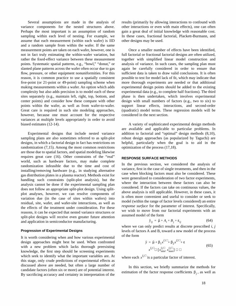
18

Several assumptions are made in the analysis ofvariance components for the nested structures above.Perhaps the most important is an assumption of randomsampling within each level of nesting. For example, weassume that each measurement (within each wafer) is IIDand a random sample from within the wafer. If the samemeasurement points are taken on each wafer, however, one isnot in fact truly estimating the within-wafer variation, butrather the fixed-effect variance between these measurementpoints. Systematic spatial patterns, e.g., “bowl,” “donut,” orslanted plane patterns across the wafer often occur due to gasflow, pressure, or other equipment nonuniformities. For thisreason, it is common practice to use a spatially consistentfive-point (or 21-point or 49-point) sampling scheme whenmaking measurements within a wafer. An option which addscomplexity but also adds precision is to model each of thesesites separately (e.g., maintain left, right, top, bottom, andcenter points) and consider how these compare with otherpoints within the wafer, as well as from wafer-to-wafer.Great care is required in such site modeling approaches,however, because one must account for the respectivevariances at multiple levels appropriately in order to avoidbiased estimates (12-14).

Experimental designs that include nested variancesampling plans are also sometimes referred to as split-plotdesigns, in which a factorial design in fact has restrictions onrandomization (7,15). Among the most common restrictionsare those due to spatial factors, and spatial modeling likewiserequires great care (16). Other constraints of the “real”world, such as hardware factors, may make completerandomization infeasible due to the time and cost ofinstalling/removing hardware (e.g., in studying alternativegas distribution plates in a plasma reactor). Methods exist forhandling such constraints (split-plot analysis), but theanalysis cannot be done if the experimental sampling plandoes not follow an appropriate split-plot design. Using split-plot analyses, however, we can resolve components ofvariation due (in the case of sites within wafers) intoresidual, site, wafer, and wafer-site interactions, as well asthe effects of the treatment under consideration. For thesereasons, it can be expected that nested variance structures orsplit-plot designs will receive even greater future attentionand application in semiconductor manufacturing.

Progression of Experimental Designs

It is worth considering when and how various experimentaldesign approaches might best be used. When confrontedwith a new problem which lacks thorough preexistingknowledge, the first step should be screening experimentswhich seek to identify what the important variables are. Atthis stage, only crude predictions of experimental effects asdiscussed above are needed, but often a large number ofcandidate factors (often six or more) are of potential interest.By sacrificing accuracy and certainty in interpretation of the

results (primarily by allowing interactions to confound withother interactions or even with main effects), one can oftengain a great deal of initial knowledge with reasonable cost.In these cases, fractional factorial, Plackett-Burmann, andother designs may be used.

Once a smaller number of effects have been identified,full factorial or fractional factorial designs are often utilized,together with simplified linear model construction andanalysis of variance. In such cases, the sampling plan mustagain be carefully considered in order to ensure thatsufficient data is taken to draw valid conclusions. It is oftenpossible to test for model lack of fit, which may indicate thatmore thorough experiments are needed or that additionalexperimental design points should be added to the existingexperimental data (e.g., to complete half fractions). The thirdphase is then undertaken, which involves experimentaldesign with small numbers of factors (e.g., two to six) tosupport linear effects, interactions, and second-order(quadratic) model terms. These regression models will beconsidered in the next section.

A variety of sophisticated experimental design methodsare available and applicable to particular problems. Inaddition to factorial and “optimal” design methods (8,10),robust design approaches (as popularized by Taguchi) arehelpful, particularly when the goal is to aid in theoptimization of the process (17,18).

RESPONSE SURFACE METHODS

In the previous section, we considered the analysis ofvariance, first in the case of single treatments, and then in thecase when blocking factors must also be considered. Thesewere generalized to consideration of two factor experiments,where the interaction between these factors can also beconsidered. If the factors can take on continuous values, theabove analysis is still applicable. However, in these cases, itis often more convenient and useful to consider or seek tomodel (within the range of factor levels considered) an entireresponse surface for the parameter of interest. Specifically,we wish to move from our factorial experiments with anassumed model of the form

(64)

where we can only predict results at discrete prescribed i, jlevels of factors A and B, toward a new model of the processof the form

(65)

where each is a particular factor of interest.

In this section, we briefly summarize the methods forestimation of the factor response coefficients , as well as

yij µ Ai B j εij+ + +=

y µ β1x1( ) β2x

2( ) ε+ + +=

xj( )

xminj( )

xmaxj( ),[ ] ℜ∈ ∈

xj( )

β j

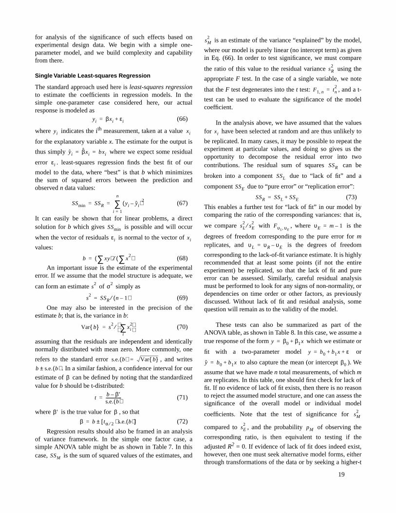
19

for analysis of the significance of such effects based onexperimental design data. We begin with a simple one-parameter model, and we build complexity and capabilityfrom there.

Single Variable Least-squares Regression

The standard approach used here is least-squares regressionto estimate the coefficients in regression models. In thesimple one-parameter case considered here, our actualresponse is modeled as

(66)

where indicates the ith measurement, taken at a value

for the explanatory variable x. The estimate for the output is

thus simply where we expect some residual

error . least-squares regression finds the best fit of our

model to the data, where “best” is that b which minimizesthe sum of squared errors between the prediction andobserved n data values:

(67)

It can easily be shown that for linear problems, a directsolution for b which gives is possible and will occur

when the vector of residuals is normal to the vector of

values:

(68)

An important issue is the estimate of the experimentalerror. If we assume that the model structure is adequate, we

can form an estimate of simply as

(69)

One may also be interested in the precision of theestimate b; that is, the variance in b:

(70)

assuming that the residuals are independent and identicallynormally distributed with mean zero. More commonly, one

refers to the standard error , and writes

. In a similar fashion, a confidence interval for our

estimate of can be defined by noting that the standardizedvalue for b should be t-distributed:

(71)

where is the true value for , so that

(72)

Regression results should also be framed in an analysisof variance framework. In the simple one factor case, asimple ANOVA table might be as shown in Table 7. In thiscase, is the sum of squared values of the estimates, and

is an estimate of the variance “explained” by the model,

where our model is purely linear (no intercept term) as givenin Eq. (66). In order to test significance, we must compare

the ratio of this value to the residual variance using the

appropriate F test. In the case of a single variable, we note

that the F test degenerates into the t test: , and a t-

test can be used to evaluate the significance of the modelcoefficient.

In the analysis above, we have assumed that the valuesfor have been selected at random and are thus unlikely to

be replicated. In many cases, it may be possible to repeat theexperiment at particular values, and doing so gives us theopportunity to decompose the residual error into twocontributions. The residual sum of squares can be

broken into a component due to “lack of fit” and a

component due to “pure error” or “replication error”:

(73)

This enables a further test for “lack of fit” in our model bycomparing the ratio of the corresponding variances: that is,

we compare with , where is the

degrees of freedom corresponding to the pure error for mreplicates, and is the degrees of freedom

corresponding to the lack-of-fit variance estimate. It is highlyrecommended that at least some points (if not the entireexperiment) be replicated, so that the lack of fit and pureerror can be assessed. Similarly, careful residual analysismust be performed to look for any signs of non-normality, ordependencies on time order or other factors, as previouslydiscussed. Without lack of fit and residual analysis, somequestion will remain as to the validity of the model.

These tests can also be summarized as part of theANOVA table, as shown in Table 8. In this case, we assume atrue response of the form which we estimate or

fit with a two-parameter model or

to also capture the mean (or intercept ). We

assume that we have made n total measurements, of which mare replicates. In this table, one should first check for lack offit. If no evidence of lack of fit exists, then there is no reasonto reject the assumed model structure, and one can assess thesignificance of the overall model or individual model

coefficients. Note that the test of significance for

compared to , and the probability of observing the

corresponding ratio, is then equivalent to testing if the

adjusted R2 = 0. If evidence of lack of fit does indeed exist,however, then one must seek alternative model forms, eitherthrough transformations of the data or by seeking a higher-t

yi βxi εi+=

yi xi

yi βxi bxi= =

εi

SSmin SSR yi yi–( )2

i 1=

n

∑= =

SSmin

εi xi

b xy∑( ) x2∑( )⁄=

s2 σ2

s2

SSR n 1–( )⁄=

Var b{ } s2

xi2

i∑

⁄=

s.e. b( ) Var b{ }=

b s.e. b( )±β

tb β′–s.e. b( )----------------=

β′ β

β b tα 2⁄ s.e. b( )⋅[ ]±=

SSM

sM2

sR2

F1 n, tn2

=

xi

SSR

SSL

SSE

SSR SSL SSE+=

sL2

sE2⁄ FυL υE, υE m 1–=

υL υR υE–=

y β0 β1x+=

y b0 b1x ε+ +=

y b0 b1x+= β0

sM2

sE2

pM

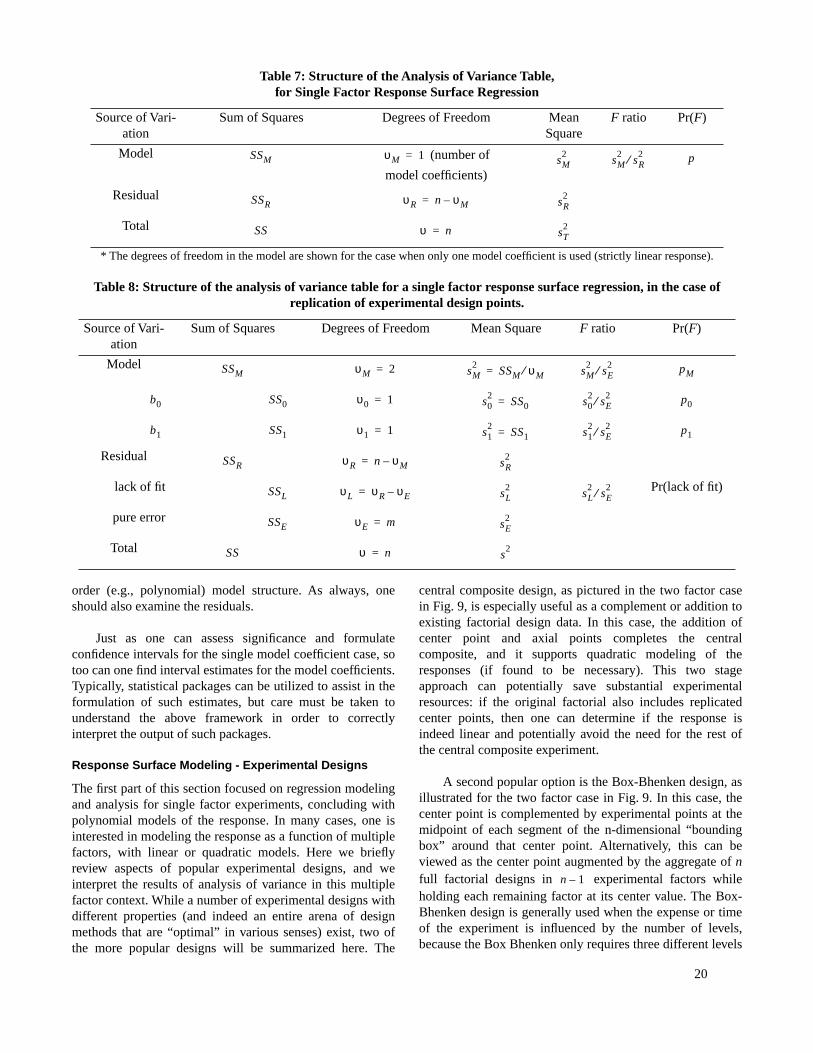
20

order (e.g., polynomial) model structure. As always, oneshould also examine the residuals.

Just as one can assess significance and formulateconfidence intervals for the single model coefficient case, sotoo can one find interval estimates for the model coefficients.Typically, statistical packages can be utilized to assist in theformulation of such estimates, but care must be taken tounderstand the above framework in order to correctlyinterpret the output of such packages.

Response Surface Modeling - Experimental Designs

The first part of this section focused on regression modelingand analysis for single factor experiments, concluding withpolynomial models of the response. In many cases, one isinterested in modeling the response as a function of multiplefactors, with linear or quadratic models. Here we brieflyreview aspects of popular experimental designs, and weinterpret the results of analysis of variance in this multiplefactor context. While a number of experimental designs withdifferent properties (and indeed an entire arena of designmethods that are “optimal” in various senses) exist, two ofthe more popular designs will be summarized here. The

central composite design, as pictured in the two factor casein Fig. 9, is especially useful as a complement or addition toexisting factorial design data. In this case, the addition ofcenter point and axial points completes the centralcomposite, and it supports quadratic modeling of theresponses (if found to be necessary). This two stageapproach can potentially save substantial experimentalresources: if the original factorial also includes replicatedcenter points, then one can determine if the response isindeed linear and potentially avoid the need for the rest ofthe central composite experiment.

A second popular option is the Box-Bhenken design, asillustrated for the two factor case in Fig. 9. In this case, thecenter point is complemented by experimental points at themidpoint of each segment of the n-dimensional “boundingbox” around that center point. Alternatively, this can beviewed as the center point augmented by the aggregate of nfull factorial designs in experimental factors whileholding each remaining factor at its center value. The Box-Bhenken design is generally used when the expense or timeof the experiment is influenced by the number of levels,because the Box Bhenken only requires three different levels

Table 7: Structure of the Analysis of Variance Table,for Single Factor Response Surface Regression

Source of Vari-ation

Sum of Squares Degrees of Freedom Mean Square

F ratio Pr(F)

Model (number of

model coefficients)

Residual

Total

* The degrees of freedom in the model are shown for the case when only one model coefficient is used (strictly linear response).

Table 8: Structure of the analysis of variance table for a single factor response surface regression, in the case of replication of experimental design points.

Source of Vari-ation

Sum of Squares Degrees of Freedom Mean Square F ratio Pr(F)

Model

Residual

lack of fit Pr(lack of fit)

pure error

Total

SSM υM 1= sM2

sM2

sR2⁄ p

SSR υR n υM–= sR2

SS υ n= sT2

SSM υM 2= sM2

SSM υM⁄= sM2

sE2⁄ pM

b0 SS0 υ0 1= s02

SS0= s02

sE2⁄ p0

b1 SS1 υ1 1= s12

SS1= s12

sE2⁄ p1

SSR υR n υM–= sR2

SSL υL υR υE–= sL2

sL2

sE2⁄

SSE υE m= sE2

SS υ n= s2

n 1–

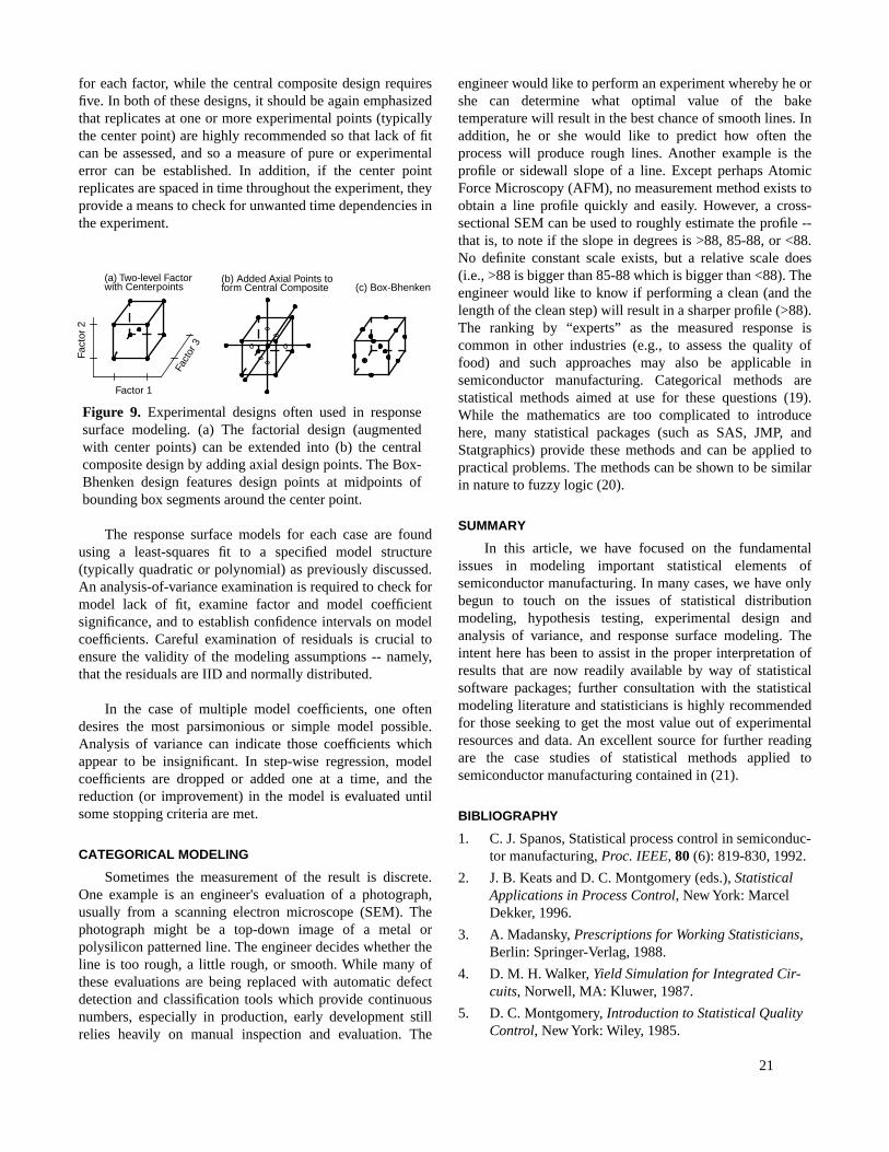
21

for each factor, while the central composite design requiresfive. In both of these designs, it should be again emphasizedthat replicates at one or more experimental points (typicallythe center point) are highly recommended so that lack of fitcan be assessed, and so a measure of pure or experimentalerror can be established. In addition, if the center pointreplicates are spaced in time throughout the experiment, theyprovide a means to check for unwanted time dependencies inthe experiment.

The response surface models for each case are foundusing a least-squares fit to a specified model structure(typically quadratic or polynomial) as previously discussed.An analysis-of-variance examination is required to check formodel lack of fit, examine factor and model coefficientsignificance, and to establish confidence intervals on modelcoefficients. Careful examination of residuals is crucial toensure the validity of the modeling assumptions -- namely,that the residuals are IID and normally distributed.

In the case of multiple model coefficients, one oftendesires the most parsimonious or simple model possible.Analysis of variance can indicate those coefficients whichappear to be insignificant. In step-wise regression, modelcoefficients are dropped or added one at a time, and thereduction (or improvement) in the model is evaluated untilsome stopping criteria are met.

CATEGORICAL MODELING

Sometimes the measurement of the result is discrete.One example is an engineer's evaluation of a photograph,usually from a scanning electron microscope (SEM). Thephotograph might be a top-down image of a metal orpolysilicon patterned line. The engineer decides whether theline is too rough, a little rough, or smooth. While many ofthese evaluations are being replaced with automatic defectdetection and classification tools which provide continuousnumbers, especially in production, early development stillrelies heavily on manual inspection and evaluation. The

engineer would like to perform an experiment whereby he orshe can determine what optimal value of the baketemperature will result in the best chance of smooth lines. Inaddition, he or she would like to predict how often theprocess will produce rough lines. Another example is theprofile or sidewall slope of a line. Except perhaps AtomicForce Microscopy (AFM), no measurement method exists toobtain a line profile quickly and easily. However, a cross-sectional SEM can be used to roughly estimate the profile --that is, to note if the slope in degrees is >88, 85-88, or <88.No definite constant scale exists, but a relative scale does(i.e., >88 is bigger than 85-88 which is bigger than <88). Theengineer would like to know if performing a clean (and thelength of the clean step) will result in a sharper profile (>88).The ranking by “experts” as the measured response iscommon in other industries (e.g., to assess the quality offood) and such approaches may also be applicable insemiconductor manufacturing. Categorical methods arestatistical methods aimed at use for these questions (19).While the mathematics are too complicated to introducehere, many statistical packages (such as SAS, JMP, andStatgraphics) provide these methods and can be applied topractical problems. The methods can be shown to be similarin nature to fuzzy logic (20).

SUMMARY

In this article, we have focused on the fundamentalissues in modeling important statistical elements ofsemiconductor manufacturing. In many cases, we have onlybegun to touch on the issues of statistical distributionmodeling, hypothesis testing, experimental design andanalysis of variance, and response surface modeling. Theintent here has been to assist in the proper interpretation ofresults that are now readily available by way of statisticalsoftware packages; further consultation with the statisticalmodeling literature and statisticians is highly recommendedfor those seeking to get the most value out of experimentalresources and data. An excellent source for further readingare the case studies of statistical methods applied tosemiconductor manufacturing contained in (21).

BIBLIOGRAPHY

1. C. J. Spanos, Statistical process control in semiconduc-tor manufacturing, Proc. IEEE, 80 (6): 819-830, 1992.

2. J. B. Keats and D. C. Montgomery (eds.), Statistical Applications in Process Control, New York: Marcel Dekker, 1996.

3. A. Madansky, Prescriptions for Working Statisticians, Berlin: Springer-Verlag, 1988.

4. D. M. H. Walker, Yield Simulation for Integrated Cir-cuits, Norwell, MA: Kluwer, 1987.

5. D. C. Montgomery, Introduction to Statistical Quality Control, New York: Wiley, 1985.

Figure 9. Experimental designs often used in responsesurface modeling. (a) The factorial design (augmentedwith center points) can be extended into (b) the centralcomposite design by adding axial design points. The Box-Bhenken design features design points at midpoints ofbounding box segments around the center point.

Factor 1

Fact

or 2

(b) Added Axial Points toform Central Composite (c) Box-Bhenken

Fact

or 3

(a) Two-level Factorwith Centerpoints

22

6. R. G. Miller, Jr., Beyond ANOVA - Basics of applied statistics, New York: Chapman & Hall, 1997.

7. G. A. Milliken and D. E. Johnson, Analysis of Messy Data, Volume I: Designed Experiments, New York: Chapman & Hall, 1992.

8. G. E. P. Box, W. G. Hunter, and J. S. Hunter, Statistics for Experimenters, New York: Wiley, 1978.

9. D. Drain, Statistical Methods for Industrial Process Control, New York: Chapman & Hall, 1997.

10. D. Drain, Handbook of Experimental Methods for Pro-cess Improvement, New York: Chapman & Hall, 1997.

11. R. K. Burdick, F. A. Graybill, Confidence Intervals on Variance Components, New York: Marcel Dekker, 1992.

12. T. H. Smith et al., Bias and variance in single and mul-tiple response surface modeling, Third Int. Workshop Stat, Met.: 60-63, Honolulu, HI, 1998.

13. R. Guo and E. Sachs, Modeling, optimization, and con-trol of spatial uniformity in manufacturing processes, IEEE Trans. Semi. Manuf., 6 (1): 41-57, 1993.

14. P. K. Mozumder and L. M. Lowenstein, Method for semiconductor process optimization using functional representations of spatial variations and selectivity, IEEE Trans. Comp. Hybrids, Manuf. Tech., 15 (3): 311-316, 1992.

15. R. L. Mason, R. F. Gunst, and J. L. Hess, Statistical Design and Analysis of Experiments with Applications to Engineering and Science, New York: Wiley; 1989.

16. B. D. Ripley, Spatial Statistics, New York: Wiley, 1981.

17. P. J. Ross, Taguchi Techniques for Quality Engineering, 2nd ed., New York: McGraw-Hill, 1996.

18. M. S. Phadke, Quality Engineering Using Robust Design, Englewood Cliffs, NJ: Prentice Hall, 1989.

19. A. Agresti, Categorical Data Analysis, New York: Wiley, 1990.

20. C. Spanos and R. Chen, Using Qualitative Observa-tions for Process Tuning and Control, IEEE Trans. Semi. Manuf., 10 (2): 307-316, 1997.

21. V. Czitrom and P. D. Spagon, (eds.), Statistical Case Studies for Industrial Process Improvement, Philadel-phia: ASA-SIAM, 1997.