THE NATURE AND PERFORMANCE OF REVERSE MERGERS

Chi Sun

A Thesis

in

The John Molson School of Business

Presented in Partial Fulfillment of the Requirements

for the Degree of Master of Science in Administration (Finance) at

Concordia University

Montreal, Quebec, Canada

November 2008

© Chi Sun, 2008

1*1 Library and Archives Canada

Published Heritage Branch

Biblioth&que et Archives Canada

Direction du Patrimoine de l'6dition

395 Wellington Street Ottawa ON K1A0N4 Canada

395, rue Wellington Ottawa ON K1A 0N4 Canada

Your file Votre reference ISBN: 978-0-494-63233-8 Our file Notre reference ISBN: 978-0-494-63233-8

NOTICE:

The author has granted a non-exclusive license allowing Library and Archives Canada to reproduce, publish, archive, preserve, conserve, communicate to the public by telecommunication or on the Internet, loan, distribute and sell theses worldwide, for commercial or non-commercial purposes, in microform, paper, electronic and/or any other formats.

The author retains copyright ownership and moral rights in this thesis. Neither the thesis nor substantial extracts from it may be printed or otherwise reproduced without the author's permission.

AVIS:

L'auteur a accorde une licence non exclusive permettant a la Bibliotheque et Archives Canada de reproduire, publier, archiver, sauvegarder, conserver, transmettre au public par telecommunication ou par I'lnternet, preter, distribuer et vendre des theses partout dans le monde, a des fins commerciales ou autres, sur support microforme, papier, electronique et/ou autres formats.

L'auteur conserve la propriete du droit d'auteur et des droits moraux qui protege cette these. Ni la these ni des extraits substantiels de celle-ci ne doivent etre imprimes ou autrement reproduits sans son autorisation.

In compliance with the Canadian Privacy Act some supporting forms may have been removed from this thesis.

While these forms may be included in the document page count, their removal does not represent any loss of content from the thesis.

Conformement a la loi canadienne sur la protection de la vie privee, quelques formulaires secondaires ont ete enleves de cette these.

Bien que ces formulaires aient inclus dans la pagination, il n'y aura aucun contenu manquant.

1 * 1

Canada

ABSTRACT

The nature and performance of reverse mergers

Chi Sun

I compare a sample of reverse mergers between 1995 and 2006 with comparable mergers

of public firms and acquisitions of public targets by private firms. I find that reverse

merger and going private transactions target firms with different characteristics. The short

horizon stock price performance upon announcement of reverse mergers is correlated

with the termination fee and time to effectuate the transaction. Finally, consistent with

prior research, reverse mergers result in long-run stock price underperformance. However,

the magnitude of this underperformance is small and it is not accompanied by significant

operating underperformance.

iii

ACKNOWLEDGEMENTS

I am very grateful to my thesis supervisor, Dr. Nilanjan Basu. I would like to thank

him for guiding and supporting me in my thesis. I really appreciate his time, effort and

prompt responses to my questions and especially his patient directing.

I would also like to thank my committee members, Dr. Sandra Betton and Dr.

Yaxuan Qi for their precious recommendations and suggestions on my thesis.

And finally, I would like to thank my family members and my friend Haibo Jiang

for their encouragement and constant support. Their appreciation, acknowledgement and

confidence drive me to reach my best.

iv

TABLE OF CONTENTS

List of Figures vii

List of Tables viii

I. Introduction 1

II. What is Reverse Merger 3

2.1 Definition 3

2.2 The reverse merger process 4

2.3 Advantages offered by reverse mergers 5

III. Reverse mergers as mergers 6

IV. Hypothesis development 9

V Data Description 12

VI. Methodology and Results 14

6.1 Univariate Analysis 14

6.2 Multivariate Logit analysis 16

6.3 Event Study 18

6.3.1 Cumulative Abnormal Returns 18

6.3.2 Multivariate Regression on CARs 20

6.4 Post-event Long-Term Analysis 21

6.4.1 Buy-and-Hold Returns 21

v

6.4.2 Fama-French Three Factor Regression 23

6.4.3 Accounting and Operating Performance 25

6.4.4 Equity and debt issues 26

VII. Conclusion 27

Reference 29

Appendix A 47

vi

LIST OF FIGURES

Figure 1: Post-event two year change in balance sheet liquidity 32

Figure 2: Post-event two year change in balance sheet leverage 32

vii

LIST OF TABLES

Table 1: Sample descriptive statistics 33

Table 2: Firm and Deal characteristics in year prior to going public 34

Table 3: Correlation Matrix 36

Table 4: Logit regressions of transaction targets 37

Table 5: Cumulative Abnormal Returns 38

Table 6: Robustness test for CAR 39

Table 7: Multivariate regression of 3-day (-1, +1) CAR 40

Table 8: Post-event return performance - BHRs and BHARs 41

Table 9: Calendar - Time Portfolio Regression 42

Table 10: Accounting and Operating performance of post-event time period 44

Table 11: Accounting and Operating performance of post-event time period 46

Appendix A 47

viii

I. Introduction

The New York Stock Exchange (NYSE) became possibly the most well known

example of a reverse merger when, on April 21, 2005, it announced its plan to go public

via a reverse merger with Archipelago Holdings Inc. Such a reverse merger (RM)

combines elements of an initial public offering (IPO) as well as a merger in that it permits

a private firm to go public through a merger rather than an offering of shares.1 Since the

early 1980s, the reverse merger has become an increasingly popular way for private firms

to access the capital markets.2 However, although IPOs and mergers have been

extensively analyzed by researchers, reverse mergers, which combine elements of both,

are not as well understood. A notable exception is the work of Gleason, Rosenthal and

Wiggins (2005), who find that reverse mergers are followed by poor operating

performance. They also find that a substantial number of firms undertaking reverse

mergers do not survive for two years. They conclude that reverse mergers may have

failed to generate value for shareholders.

The analysis of Gleason, Rosenthal and Wiggins (2005), like much of the existing

research on reverse mergers, focuses exclusively on a comparison of reverse mergers

with similar IPOs.3 To the best of my knowledge, there have been no research studies that

have examined reverse mergers by comparing them to other mergers. Yet, a reverse

merger has as much in common with mergers as it does with IPOs. This raises two

potential concerns with existing research. First, a comparison with IPOs would tend to

1 In order to differentiate them, I will refer to mergers that are not reverse mergers as "regular mergers" 2 Gleason, Jain and Rosenthal (2005) report three reverse mergers between 1984 and 1989, 40 between 1990 and 1995, and 75 between 1996 and 2001. 3 Others who have worked on this topic include, Arellano-Ostoa and Brusco (2002), Gleason Jain and Rosenthal (2005) and Adjei, Cyree and Walker (2008).

1

ignore certain deal specific features that influence the performance of reverse mergers. In

support of this I find that the abnormal returns associated with a reverse merger are

significantly negatively related to termination fees and the time between the

announcement date and the effective date of the merger. In contrast the relationship

between termination fee and announcement returns is insignificant for regular mergers.

My findings complement those of Officer (2003) and suggest that termination fees play a

different role in reverse mergers than they do in regular mergers.

Second, the conclusions based on a comparison of RMs with IPOs could be

misleading in that acquiring firms in reverse mergers will share the characteristics of a

regular merger as much as other types of mergers. I propose to remedy this shortcoming

by testing the performance of reverse mergers against a benchmark of regular mergers

and going private (GP) transactions.4 Although I am unable to uncover any significant

difference in short horizon abnormal returns for reverse mergers, I find that over 1 2 - 3 6

months, the stock price performance of reverse mergers trails that of comparable regular

mergers. In addition, the operating performance of firms participating in reverse mergers

is poorer than that showed by comparable public merging firms. The evidence suggests

that although RM firms are not initially penalized by the market, they have delivered

poor returns over the longer term. Finally, private firms that acquire public firms in

reverse mergers appear to have higher leverage and less cash than their public

counterparts.5 Overall, my findings are largely consistent with existing research in that I

find that RMs result in poor long term performance. However, the magnitude of the

4 Going private transactions are defined as ones in which a private firm or a group of investors acquires a public firm and the merged entity is not publicly traded. 5 From here on, I refer to the private firm involved in a reverse merger as the acquirer and the public firm as the target.

2

underperformance is small. The rest of this paper is organized as follows. Section 2

defines and describes the features of a reverse merger. Section 3 examines the merits of

analyzing RMs against a benchmark of mergers. Section 4 develops the hypotheses.

Section 5 explains the data and the sample selection method. Section 6 discusses the

methodology and results. Section 7 concludes this paper.

II. What is Reverse Merger?

2.1. Definition

In a reverse merger, a private firm acquires a public firm, and through the acquisition,

it obtains listing in a specific stock exchange. Thus, public firms listed in New York

Stock Exchange (NYSE), American Stock Exchange (AMEX) and other major stock

exchanges, as well as those listed in Over-the-Counter Bulletin Board (OTCBB) or Pink

Sheets are possible targets for private firms seeking RM opportunities. Although RM

transactions can typically be completed in a matter of weeks, many take months or even

years to complete. As in a regular merger, the public firm in a RM is required to submit

relevant filings, such as 8-Ks to Securities and Exchange Commission (SEC), and the

submission of paperwork must be completed two weeks before the transaction closes. A

RM can be considered completed when the private firm controls the majority of the

public firm's shares. Usually, the transaction involves the reorganization of former public

firm with respect to its capital structure, ownership structure, and board composition.

3

2.2. The reverse merger process

A RM is commonly undertaken through a process called "Reverse Triangular

Merger", especially for those public companies traded in OTC or Pink Sheet. A typical

Reverse Triangular Merger consists of several steps:

1) The public firm creates a wholly owned shell subsidiary;

2) This subsidiary is then merged into the private firm;

3) The subsidiary is the surviving firm nominally, while it is the shareholders of the

(former) private company that control the surviving subsidiary;

4) Shares of the private firm are exchanged for shares of the public firm. This step is

the key step whereby the public company (parent) issues new shares in exchange

for shares in the private firm (subsidiary). The newly issued shares will typically

account for a majority (greater than 50%) of all diluted outstanding shares of the

public firm.

5) The private firm becomes a wholly-owned subsidiary of the public company

while the shareholders of the (former) private firm own the majority of the now

merged public firm's shares.

6) In a later phase, the public firm may replace its board members and management

team with those of the private firm.

4

Although RMs can be structured through a direct merger, in which the former public

firm directly merges with the private firm, the "Reverse Triangular Merger" can be a way

to lower the costs of finalizing the merger.6

2.3. Advantages offered by reverse mergers

IPOs, as opposed to RMs, result in directly raising fund by issuing stocks. In contrast,

RMs take two steps to get to the same place as IPOs. First, the RM firm buys and merges

with a public shell company and obtains the public listing; second, the merged entity

arranges for investors to purchase its stock or raises financing through alternative means.

These could include debt financing, factoring arrangements, traditional private

placements, PIPEs (private investment in public equity), or venture capital financing. .

Feldman (2006) documented several advantages offer by RM: 1) lower cost; 2)

speedier process; 3) less time-consuming for company executives; 4) not dependent on

IPO market and 5) underwriter unnecessary. In addition, he argued that PIPE is an

important way of financing for RM firms as "...PIPE investors such as hedge funds are

often able to lock in gains on PIPE investments as a result of favorable deal terms and

short selling regardless of how the company's stock performs post-deal". The PIPE is not

an option for private firms to financing. However, the RM opens up a PIPE option for

6 Feldman (2006) and Sjostrom (2008) point out that the Reverse Triangular Merger can avoid the time and expense involved in obtaining approval from the shell firms' shareholders, as well as those associated with SEC filings. Feldman (2006) points out that another advantage is that a Reverse Triangular Merger does not change any of the existing contracts associated with the operating company (i.e. private company) and thus leads to minimal disruption. 7 See Feldman (2006).

5

• 8

private firms who are small, not meeting the requirements of IPO listing but also in need

of fund as greatly as IPO firms.

Ill Reverse mergers as mergers

Prior research has largely considered the reverse merger as an alternative way (as

opposed to the IPO) of going public by which the "ready-to-go-public" private firm may

obtain a public listing in a shorter time. Gleason, Rosenthal and Wiggins (2005) examine

121 reverse merger cases and find little evidence of any improvements in operating

performance following the merger. Further, only 46% of their sample survives two years

after the reverse merger. It is important to note that their analysis benchmarks reverse

mergers against IPOs. However, analyzing reverse mergers purely as a mechanism of

going public may not provide us with the full picture for several reasons.

First, there are several significant differences between an RM and an IPO in terms of

the role of the investment bank. In an IPO, underwriters are involved in the issuance of

the firm's security and they are authorized to manage the sale of securities to the public

(Ritter, 2003). Underwriters and investment banks could play a key role in the process: in

that 1) They assist IPO firms in deciding which kind(s) of securities are going to be

issued (such as common stocks and preferred stocks)(Feldman, 2006); 2) They assist IPO

firms in determining the issue price as well as the timing of the decision to issue

securities. As a result, the reputations and efforts of underwriters and investment banks

could influence the outcome of IPOs.

8 See Sjostrom (2008)

6

Prior research confirms that investment banks play a significant role in an IPO. For

example, Carter and Manaster (1990) argue that underwriters with higher prestige are

associated with lower risk offerings. In addition, the efforts and prestige of underwriters,

could affect the stock price performance even after the issuance. Carter, Dark and Singh

(1998) found that IPOs managed by more reputable underwriters are associated with less

short-run under-pricing and less severe long-term (3 year holding period) under-

performance. Ellis, Michaely and O'Hara (2000) examine the aftermarket trading activity

of underwriters and conclude that the lead underwriter is always the dominant market

maker and that the lead underwriter continues to engage in stabilization activity for less

successful IPOs and to make efforts to reduce risk. In contrast, investment banks or

underwriters put little or no effort (as compared to IPOs) on RM transactions, and they

appear to have no willingness or obligation to make an active secondary market for RM

securities.

Prior research on RM firms does not provide much evidence of support from

investment banks. After RM firms obtain their public status, their shares are thinly traded

(Ewing, 2000). A possible reason behind this illiquidity could be that no underwriter is

involved in the RM and thus there is no "push" from the underwriter to activate a

secondary market for RM firms (Sjostrom, 2008). In a similar spirit, James (2007) states

that "...the shares of the public shell may not even be then currently trading on any

securities exchange or quotation system". So, post-RM firms do not benefit as much as

their IPO counterparts from investment bank support. Moreover, securities of post-RM

firms are usually rated as "high in risk" and "low in investment value" by analysts,

investors and financial institutions (Gleason, Jain and Rosenhal, 2005; Carpentier and

7

Suret, 2008). A possible reason is that unlike IPO firms, post-RM firms receive no

underwriter certification (Gilson and Kraakman, 1984).

Second, a reverse merger takes place through an exchange of shares while an IPO

results in an infusion of funds into the firm that goes public. As suggested by Jensen

(1986), an increase in free cash flow in the presence of the principal agent problems

could lead to a decrease in firm value. This hypothesis has received some support from

research on mergers as well as divestitures.9

Third, different regulatory standards and requirements could be associated with the

firm's accounting performance in the post-transaction period. IPO firms need to meet the

requirements set by the stock exchange. However, a reverse merger bypasses such

regulatory requirements and effectively allows some firms that do not meet such criteria

to obtain access to the financial markets10. Evidence of this difference is provided by the

work of Carpentier and Suret (2008) who examine a sample of Canadian reverse mergers

and find that the lower disclosure and compliance requirements for these firms results in

lower quality companies. They find that such firms are also more likely to delist over five

or ten years following the RM.

Fourth, many of the public firms that are acquired in a reverse merger report poor

performance prior to the RM (Gleason, Rosenthal and Wiggins, 2005). The post-RM firm,

similar to other firms involved in a merger, may face negative effects from structural

reorganization and recapitalization. This is not a challenge for IPO firms.

9 See, for example, Harford (1999) and Allen and McConnell (1997) for evidence on the relationship between cash availability and value. 10 For example, NYSE sets standards those IPO firm needs to have minimum $2 million of earnings each of the 2 most recent years or $75 million revenues of the most recent fiscal year in order to get a public listing. However, the requirements for maintain an existing listing are not as stringent.

8

Finally, several researchers have pointed out the positive or negative synergies

associated with mergers. For example, Gugler et. al. (2002) argue that conglomerate

mergers decrease sales more than horizontal mergers and Farrell and Shapiro (1990)

show that merger synergies are inversely related to prices. It is unclear to what extent

such positive or negative synergies could affect a specific reverse merger. However, they

could be the reason for systematic differences between reverse mergers and IPOs.

IV. Hypothesis development

Prior literature on reverse mergers has largely concluded that these transactions are

poor performers, both in terms of accounting and stock returns. By comparing RM to

IPOs, these studies come to the conclusion that the RM is a risky way of going public.

For example, Gleason, Rosenthal and Wiggins (2005) suggest that RMs may fail to

generate revenues; Gleason, Jain and Rosenthal (2005) find that RM firms are smaller

and have lower levels of profitability as well as larger declines in profitability than

comparable IPOs; Adjei et al. (2008) examine the issue of survival during the post-RM

period and find that 42% of RMs are delisted within 3 years of listing on an exchange. In

contrast, only 27% of similar IPO firms are delisted in the three years following the IPO.

However, as I have argued, comparing reverse mergers to IPOs runs the risk of

overlooking their role as mergers. Moreover, I would expect that private firms using RM

gain short-run benefits otherwise they would not choose to undertake this process. Hence

my null hypothesis is that:

9

HI: "The operating and stock price performance of RMs will not differ from those of

regular mergers ".

Another recognized issue in prior research is that the IPO generally is a relatively

more time consuming and expensive process than the RM.11 Investment banking fees, the

cost of underpricing on the first day of trading, and the time and cost related to SEC

filings are all part of the IPO process. However, such cost could be reduced if private

firms choose RMs as the mechanism of going public.12 As such, deal specific issues can

be expected to influence the returns earned by RM participants. First, a lower

requirement of senior management time is one of the potential benefits of a reverse

merger. However, this benefit is eroded if the reverse merger process itself becomes

complex and time consuming. As such, I would expect that the speed of completion

would be related to the value of the firms undertaking a reverse merger. In addition,

unlike for regular mergers, the ease of the process is one of the main criteria for deciding

the success or otherwise of a reverse merger. As a result, although this concern should

apply to all mergers, it is possible that this will be especially significant in reverse

mergers. Second, Officer (2003) suggests that termination fees may influence merger

outcomes. Termination fees could be used by managers of the target firm to prevent

competition amongst bidders and thus allow them to lock in deals that enhance their

private benefits. Alternatively, termination fees could be used as a mechanism to induce

commitment and so facilitate the sharing of information, thereby increasing value for

shareholders. To the extent that the termination fee and the time to completion are deal

uSee, for example, Carpentier and Suret (2008) 12 See Ritter (1998), Feldman (2006) and James (2007)

10

specific characteristics, I contribute to the evidence on reverse mergers by examining

their impact on target returns. In addition, I test whether the relationship between such

deal characteristics and target returns differs between reverse mergers and regular

mergers. Thus my second null hypothesis is:

H2: "The speed of completion will not influence the value creation from a reverse

merger; the importance of this factor will be no different for reverse mergers than for

regular mergers. The termination fee associated with a reverse merger will be unrelated

to the returns earned by the target. The relationship between the termination fee and the

target returns will be the same for reverse mergers and regular mergers. "

My third hypothesis concerns financing and capital structure. Ghosh and Jain (2000)

find a significant increase in financial leverage following mergers and they show that

announcement period market-adjusted returns are positively related to increases in

financial leverage. I expect that private firms that undertake RMs do so, at least in part, to

access the public financial markets. On the other hand, private firms before using RM

also have the option to stay private. In a RM or GP transaction, the (private) acquirer has

to choose the target and to examine target's financial position with respect to the effect it

will have on the liquidity and leverage of the merged entity. In a GP transaction, the

merged entity will have limited access to the capital markets and so the combined

liquidity of the merged entity may be a more vital concern than in the case of RMs.

Thus I have my third null hypothesis:

H3: "RM targets and GP targets will not differ in terms of liquidity and leverage ".

11

V. Data Description

I obtain my initial sample of Reverse Mergers from Securities Data Corporation's

(SDC) Mergers and Acquisition database. I search SDC for all reverse merger

transactions between 1995 and 2006 where: 1) Acquirers and targets are restricted to US

firms; 2) Merger transactions involve one private firm and one public firm and the merger

is initiated by the private firm; 3) The transaction is not a tender offer, a hostile merger,

or a leveraged buyout and; 4) The transaction is completed13.

However, SDC often defines RMs incorrectly, and this results in a bigger RM

sample that incorrectly includes other kinds of firm combinations (e.g. rollups and regular

acquisition). In addition, SDC sometimes reports the announcement date of a certain

event inaccurately. For these reasons, I confirm my sample using data from proxy

statements, 8-Ks and other related SEC filings from the EDGAR database as well as

news releases obtained from Lexis-Nexis and Factiva. I also ensure that after the merger,

the former private shareholders own more than 50% of the shares of the merged public

entity. The exact date of announcement is verified through Lexis-Nexis and Factiva. My

final sample consists of 171 reverse mergers. Of these I am able to find operating

information for 146 firms from SEC filings and Compustat. Merging with stock price

data from Center for Research in Stock Price (CRSP) reduces the sample size to 68. A

possible reason why there are only 68 firms having price information available is that

most of the RM firms are traded on the OTC or Pink Sheets after the merger, while CRSP

13Typically, in a reverse merger, the former public board of directors appoints a new CEO for the new company who served as the former private firm's CEO and/or owns the private firm, and in some circumstances, several board members are introduced to the board of directors and most of them are from the private firm. Also, the newly combined firm normally abandons the public firm's name and takes the former private firm's name (although this step is not necessary to define a reverse merger).

12

only includes stocks that are traded on NYSE, AMEX and NASDAQ stock exchanges.

Finally, I remove 4 firms in the financial services sector (SIC 6000 - 6999) leading to a

final sample size of 64.

Like RMs, GP transactions also involve one private firm and one public firm. This

process is also undertaken through a merger or acquisition and shareholders of the private

firm gain control of the post-GP firm. The major difference between GP and RM is that

after merger the GP private acquiring firm stays private and the public target delists from

the relevant stock exchange. Thus the public target firm becomes a wholly-owned

subsidiary of the private firm. To the extent that the major difference between these two

kinds of transactions is in the listed (or unlisted) nature of the merged entity, a

comparison with going private transactions may enable us to better understand the causes

and consequences of reverse mergers.

In order to analyze my sample against a comparable benchmark, I match my sample

to similar regular mergers (the acquirers are matched although I provide comparisons for

targets as well) and going-private transactions (only for targets). Unlike research on firms

that go private, my study excludes those GP acquirers which are investors or shareholders

and only examine cases where the GP acquirer is another firm.

I match each acquirer in my sample of reverse mergers to an acquirer with the same

2-digit SIC code, in the same year, and with the closest total assets that undertakes a

regular merger. In a similar fashion, I match each target in my sample of reverse mergers

to a target in a going private transaction. Thus I end up with three related samples of

reverse mergers, regular mergers and going private transactions.

13

A potential shortcoming of the above matching approach is that I use the broad 2-

digit SIC definitions and therefore may end up with an imprecise match. In order to test

for the robustness of my results, I replicate my entire analysis using samples matched by

the 4-digit SIC code. In order to avoid losing a large part of my sample due to the tighter

industry definition, I do not require that the matching transaction be in the same year. My

results remain qualitatively unchanged. I also, replicate my tests for operating

performance by including firms that have data available on Compustat but not on CRSP.

Once again my results remain qualitatively unchanged.

Details for the full sample of 64 firms are provided in Table 1. As shown in Panel A,

the most active years for RMs are after 199914. In Panel B, we report the distribution of

the 4-digit SIC codes in our sample. The largest contribution comes from firms in the SIC

codes 7000-7999 (computer hardware/software or internet related "high-tech" firms)

which account for 29.7%, and the second and third largest are from firms with SIC codes

3000-3999 (manufacturing firms) and 2000-2999 (manufacturers of household goods).

VI. Methodology and Results

6.1. Univariate analysis

I first analyze the differences in the characteristics of acquirers and targets in the year

prior to the merger to see whether there are significant difference between RMs, Regular

14 However, several reverse mergers after 1999 do not have CRPS data available. As a result, our final sample is more evenly distributed across years.

14

mergers and GPs. My results for the differences and the corresponding paired t-tests and

Wilcoxon signed rank tests are reported in Table 2.

Panel A shows mean and median values for acquirers in RMs and regular mergers.

Both types of acquirers are small firms with mean (median) total assets of $39.63 million

($12.17 million) and $47.34 million ($40.07 million).15 Although the absolute values for

the size are noticeably different, tests for size difference indicate that there is no

significant difference between the two types of acquirers.

I find that the difference in the return on assets (ROA, measured as the ratio of

earnings before interest and taxes to total assets), is only moderately significant in 10%

level for mean and not significant for median. The result is consistent with prior findings

where they also find no difference or little difference in pre-merger profitability (Adjei et

al. (2008), Aydogdu et al. (2008), and Gleason et al (2005)). Further, the lack of a

significant difference in pre-merger ROA suggests that my subsequent comparisons of

post merger changes in operating performance will not be overly influenced by mean-

reversion in measures of operating performance.16 Table 2 also reports a comparison of

leverage and liquidity for my sample. I find that there is significant difference between

acquirers in different groups. In the year prior to transaction, RM acquirers have less cash

and equivalents but more debt than their regular M&A counterparts (both significant at

the 1% level for mean and median).

15 This result is not surprising because we constructed the matching regular M&A firms by Total assets and SIC. 16 See Barber and Lyon (1997) for potential biases in measurement of operating performance when pre-event operating performance is unusually high or low.

15

Table 2 Panel B reports similar descriptive statistics for targets in RM, regular

mergers and GP transactions and provides tests of differences between the three groups.

The targets are larger than their acquirers (however, unreported t-tests and Wilcoxon tests

suggest that the difference is not significant). Also, I find similar results in terms of

profitability as acquirers. All types of targets have negative ROAs but RM targets are

significantly poorer in their performance than the other two groups. RM targets also hold

significantly less cash than regular merger targets and significantly less cash than GP

targets. As for the leverage, RM targets have more debt than M&A targets17. However,

RM targets have lower levels of leverage than GP targets (again significant at 1% level).

The results till this point suggest that the differences in operating performance,

liquidity and leverage could be related to the choice between RMs and GP transaction. I

further explore this possibility in the following sections.

6.2. Multivariate logit analysis

At the time of acquisition of a public firm by a private one, the acquirer has the

choice of retaining the private status (i.e. going private transaction) or going public

(reverse merger). This decision could influence the choice of the target as well as the way

the transaction is carried out. In order to better understand this decision I run a logistic

regression,

17 A possible reason is that firms closer to financial distress may have more debt than others. Gleason et. al (2005) found evidence that the Altman's Z (a distress proxy) is correlated with profitability (ROA and ROE).

16

p(RM or GoPrivt)

= a + pxDealV + P20wnershvp + (33Size+/34Profit+(]4Profit + psCash

+ p6Leverage

Where DealV is the deal value of the reverse merger or going private transaction,

Ownership is the percentage of new company shares held by former private firms

(acquirers), Size is measured by the log of total assets at the time of the transaction,

Profit is measured by ROA, Cash is the ratio of cash and equivalents to total assets

(which proxies for liquidity) while Leverage is the ratio of debt to total assets. In

addition, I also examine the relationship between each two of the above variables by

constructing the correlation matrix which is shown in Table 3.

The results for several alternative specifications are reported in Table 4. The

coefficient estimate for Log (Deal Value) is negative and significant, while the

coefficient estimate for Ownership is positive and significant. Taken together, they

suggest that reverse mergers involve relatively larger acquirers targeting relatively

smaller firms.

The coefficient estimates for the level of cash holdings of the target are negative and

significant, suggesting that RM targets have less cash than comparable GP targets.

Together with the observed positive coefficient for Log (Deal Value), this indicates that

the need for funds, or lack thereof, could be one of the determinants of the choice to go

private. The acquisition of a large target with significant cash holdings can result in an

indirect infusion of cash for the acquirer. As a result, GP acquirers may not have as much

need to access the capital markets and may therefore not find it as useful to be publicly

17

listed. In contrast, RM acquirers that acquire small targets with low cash holdings will not

gain any significant amounts of cash from the transaction. Therefore, acquirers in RMs

may need to access the capital markets soon after the merger and could conceivably

perceive greater value in remaining a publicly listed entity. Consistent with this idea, the

coefficient estimate for leverage is positive indicating lower unused debt capacity in the

target. However the level of significance is sensitive to the regression specification.

6.3. Event Study

6.3.1. Cumulative Abnormal Returns (CARs)

Following Brown and Warner (1985), I use daily stock returns and an estimation

period from day -210 to day -10, relative to event date to estimate the parameters for the

market model. I use the estimated parameters to compute the abnormal returns over the

(-1, 1), (0, 0), and the (-5, 5) event windows for all groups of public firms in my sample

(these consist of the targets in RM and GP transactions and the acquirers as well as

targets for regular mergers). In addition, Bouwman, Fuller and Nain (2007) suggest that

1 o

under certain conditions , the CAR computed using the market model may be biased and

a more accurate result can be obtained by using the market returns as benchmark. The

results are similar when I use the two approaches.

In Table 5, I examine the short-run market reaction to the three types of merger

transactions. Panel A reports the abnormal returns earned by various groups of firms

18 As noted by Bouwman, Fuller, and Nain (2007), the presence of frequent acquirers in a sample may suggest a high probability of other acquisition announcements during the estimation period. As a result, any abnormal returns caused by these announcements will bias the parameter estimates.

18

while panel B examines potential differences between returns earned by these groups of

firms. Consistent with prior merger literature, targets appear to earn positive returns while

acquirers earn close to zero abnormal returns. 19 For the (0, 0) window, the mean

cumulative abnormal returns (CARs) for RM targets are 8.4% and significantly different

from zero. The returns are even larger and more significant for the (-1, +1) and (-5, +5)

• 9 f t

windows. The median CAR for event date (0, 0) is somewhat smaller at 0.7% and not

statistically significantly different from zero. However, the median returns for the larger

(-5, +5) and (-1, +1) window are 5.6% and 9.4% and significant at the 5% level. Overall,

targets in reverse mergers and going private transactions appear to earn higher returns

than do their counterparts in regular mergers. For reverse mergers, it is possible that the

private acquirer is willing to pay a premium for the benefit of being able to access the

financial markets post-merger and this leads to a higher announcement return for the

public target. However, the comparison of RM targets with GP targets does not yield any

definite conclusions. I report similar results using market adjusted returns in Table 6. The

results are similar to those in Table 5.

Two factors may account for the difference in CAR between GP and regular M&A.

First, my results are consistent with the findings of Weir et al (2005) who find that firms

that go private are relatively undervalued compared to firms that do not. To the extent,

that there is a potentially greater increase in value from going private for a certain group

of firms, they would be more likely to be candidates for GP transactions and as a result

earn higher abnormal returns upon announcement of the GP transaction. Second, Gleason,

19 See, for example, Jensen and Ruback (1983), Huang and Walkling (1987) and Jarrel, Brickley and Netter (1988). 20 These are using the CRSP equally-weighted market index. The counterparts using the CRSP value weighted index are similar and also reported in Table 5.

19

Payne and Wiggenhorn (2007) find that that certain public firms can benefit from going

private and thus avoiding the higher costs of being public due to the Sarbanes-Oxley Act

of2002.

6.3.2. Multivariate regression on CARs

Following Gleason, Jain and Rosenthal (2005), I define (-1, 1) CARs as a dependent

variable and regress it on firm and deal characteristics to better understand the factors that

influence the returns earned by targets in RM, GP and regular mergers.211 report these

results in Table 7.

The independent variables include Termination Fee, Deal Value, Duration,

Ownership, Size (Total Assets and Sales), ROA, Cash (to total assets) and Debt (to total

assets). Termination fee is the amount of the charge (in million US dollars) on a party

who terminates the merger transaction prior to the effective date; Duration is the number

of days between announcement date and effective date of the transaction. The remaining

variables are as defined in Table 4 and all variables are also defined in the Appendix.

For reverse mergers, the abnormal returns earned by the target are negatively

associated with termination fees. Officer (2003) suggests two ways in which termination

fees could be related to merger outcomes. First, Termination fees could be used to lock in

"sweetheart deals" for the target managers and so could be detrimental to the interests of

the target shareholders. Alternatively, termination fees could be used as a mechanism to

induce commitment and so facilitate the sharing of information, thereby increasing value

21 We drop certain variables in Regular M&A and in GP models because of the non-availability of data.

for shareholders. My findings suggest that unlike for regular mergers, termination fees

are negatively associated with target returns.

I find that Deal Value is negatively and Ownership positively associated with

abnormal returns. Taken together, they suggest that higher returns for RM targets are

observed when the acquirer is relatively large and the target relatively small.

I find that Duration is negatively related to the abnormal returns. To the extent that

the time between announcement and completion of a merger proxies for the complexity

of the deal, it suggests that target shareholders earn higher returns when the completion

of the deal faces fewer hurdles. However, the relationship is similar for regular mergers

suggesting that this is no more an issue for RMs than it is for regular mergers.

Finally, I find that the cash holdings of the target are positively related and the

leverage of the target is negatively related to abnormal returns for GP transactions but not

for RM or regular mergers. This suggests that the market values the higher liquidity in the

target only in cases where the merged entity will not have access to the public financial

markets after the merger.

6.4. Post-event long-term analysis

6.4.1. Buy-and-hold returns

Similar to prior research, I measure long run performance using buy and hold

abnormal returns benchmarked against a portfolio of matched firms and then test for

21

99 robustness using a calendar time portfolio approach. I calculate the buy and hold returns

(BHRs) using daily returns for post-event firms and the buy-and-hold abnormal returns

(BHARs) are defined as the differences between BHRs of reverse mergers and those of

matching firms.

Ti

t=2

And

BHARit = BURgt - BHRjt

Where

Rgt = the return to stock i over day t

Tg = end of holding period f or stock i

j = the matching stock to stock i

I define several holding periods which include 6, 12, 18, 24 and 36 months following

the first day after the announcement of the merger. Because of various reasons

(bankruptcy, acquisitions, etc.), the merged entity delists from stock exchanges as time

goes on. I keep the active firms at the specified time period and calculate their BHRs.

Table 8 reports the BHRs of RM firms and matching regular M&A firms for three

years which I divide into 6 categories of 6, 12, 18, 24, 30 and 36 month periods following

the merger announcement. I also report the BHAR for the same time periods.

22 See, for example, Barber and Lyon (1997), Lyon et al. (1999), and Mitchell and Stafford (2000).

22

The results show that firms undertaking RMs significantly underperform the matched

regular M&A counterparts in the long run except for the first 6 month period (using

equal-weighted mean BHRs). I also compare median BHRs of the two samples, as the

BHRs for both groups are characterized by skewness.23 The results for the medians are

similar to those using the mean.

The BHAR is negative for all time periods and significant for all except the first six

months. Additionally, in unreported results, I find that over one-third (37.3%) of my full

sample RM firms vanished within 3 years of going public. My results suggest that overall

the RM firms perform poorly. To the extent that poor performance may preclude them

from raising further funds from the market, my results are consistent with those of

Gleason, Rosenthal and Wiggins (2005) who find that less than 20% of RMs raised

capital via public offerings and that close to half the firms did not raise funds via public

offerings or private placement. Further this consistency provides some evidence that the

documented poor performance of RM firms may not have been influenced by the choice

of IPOs rather than mergers as the benchmark.

6.4.2. Fama-French Three factor regression

For each trading day during the sample period, I form equally weighted portfolios of

all sample firms that participated in the event (announcement of a reverse merger or

regular merger) within the prior 3 years. Portfolios are rebalanced daily to drop all

companies that reach the end of their 3-year period and add all companies that enter the

23 See Purnanandam and Swaminathan (2004) who investigated the distribution of long-run IPO returns.

sample at that time. I also construct similar portfolios for 6-month, 12-month, 18-month

24-month, and 30-month periods.

Next I regress the dependent variable of portfolio excess return (Rpl ~ Rjt) on the

three Fama and French (1993) factors, as described in the following equation:

Rpt -Rft = a + P* (Rmt - Rft) + s * SMBt +fc * HMLt +spt

Where Rmt is the return on the equally-weighted index in day t; R f t is the three-

month T-bill rate in day /; &pt is the return on the portfolio on day t\ SMBt i s the return

of small-cap stocks minus the return of large-cap stocks on day t; and HML{ i s the return

of high book-to-market stocks minus the return of low book-to-market stocks on day t.

The regression yields parameter estimates of a , P , s and h. The error term in the

regression is . I mainly focus on the parameter a as an estimate of the long run

abnormal returns attributable to the event.24

In Table 9 I report the results of time-series regressions of daily portfolio returns on

three factors. Coefficients of a in comparison shows that RM firms underperform their

regular M&A counterparts by, respectively, 2, 46, 28, 17, 29 and 8 basis points for 6, 12,

18, 24, 30 and 36 month period. The differences are all statistically significant. However,

the magnitude of the difference is fairly small. This result is consistent with my BHAR

comparison which shows RM firms perform somewhat worse than regular M&A

counterparts. Overall, although I find evidence of underperformance following RMs, the

magnitude of the underperformance is small. My findings are similar to those of Gleason,

24 The results for this section do not use any bootstrap tests and are indicative in nature.

Jain and Rosenthal (2005) who find that that the long run performance of RM firms is

indistinguishable from those of IPOs.

6.4.3. Accounting and operating analysis

Following Healy, Palepu and Ruback (1992)25, Gleason, Jain and Rosenthal (2005)26

and Dechow (1994)27, I compare the operating performance (measure as the return on

assets, ROA) for post-RM and post regular merger firms for the one year before and the

two years after events. I compute all measures for the combined acquirer and target by

adding the earnings for the two firms and dividing by the combined assets. I also look at

the change in the liquidity of these firms by examining the cash to assets ratio (Cash) and

the debt to assets ratio (Leverage). As with ROA, I report statistics for the combined

acquirer and target. The event times are tabulated with reference to the effective date of

the merger. I report the results in Table 10 as well as in Figures 1 and 2.

In terms of operating performance, I observe that RM firms have poorer operating

performance pre-merger. The mean and median ROA for a RM firm are significantly

lower than their counterparts one year before the effective date of the merger. As pointed

out by Barber and Lyon (1996), operating performance measures tend to revert to the

mean. Therefore, I would expect that the difference would decrease over time. However,

I find that the difference in ROA between RM firms and regular mergers widens from

one year before to one year after the event. Thereafter, the difference shrinks. Overall,

25 Examined cash-flow returns (Cash-Flow margin) and found that merged firms outperform their industries. 26 Compared major accounting ratios for post-RM firms and post-IPO firms. 27 Investigated the features of widely used accounting ratios.

RM firms appear to be poorer performing firms than their regular M&A counterparts.

However, I am unable to find a clear trend in ROA of firms that undertake a RM when

compared to a benchmark of similar firms undertaking a regular merger.

In terms of liquidity, I observe that the mean (median) leverage for RM firms

reduces from 45% (15%) one year before the merger to 13% (2%) two years after the

merger. In contrast, the mean (median) level of cash held by firms involved in regular

mergers decreases from 31% (27%) to 22% (13%). Overall, the results indicate that firms

involved in reverse mergers experience a significant improvement in their liquidity

position in the years surrounding the transaction.

A potential concern for these results arises from the fact that prior research by Adjei

et al. (2008) has found that a significant number of RM firms drop out within three years

of the transaction. The results are consistent for my sample as well - I find that about 37%

of my sample drops out within three years from the effective date of the merger. In order

to address these concerns, I replicate my results in panel B using only the sample of firms

that survive until the end of the second year. As can be seen, the conclusions remain

qualitatively unchanged.

6.4.4. Equity and debt issues

Our results till this point indicate that RMs involve poorly performing targets and

poor operating and stock price performance for the combined entity. As such, it is unclear

why some acquirers go through with these transactions. One possible reason is that the

RM allows poorly performing firms a way to access the capital markets. As mentioned by

Feldman (2006), this could include debt financing or factoring arrangements as well as

private placements particularly in the form of private investment in public equity (PIPE),

and venture capital financing.28

In order to test whether a reverse merger, in fact, allows acquiring firms increased

access to the capital markets, I examine the post RM issuance of debt and equity by the

merged firm. I find that within 2 years after the RM, 28 of the 64 sample firms undertook

public placements all of which involved equity financing. Similarly, 28 of the 64 sample

firms undertook private placements of which 11 involved debt financing and 20 involved

equity financing (3 of these firms issued debt as well as equity). It is possible that the

remaining 8 RM entities did not require any immediate financing. Overall, my findings

indicate a significant degree of fund raising activity of which a substantial portion occurs

through private placement of debt and equity.

VII. Conclusion

In this paper, I examine firms that participate in reverse mergers. I examine the

choice of targets in such transactions as well as the stock price and operating performance

of the merged entity. Prior studies have contrasted the performance of reverse mergers

with IPOs. My study differs in that I emphasize the merger aspect of the reverse merger.

This allows me to provide a fresh perspective on this issue in two ways. First, I am able

28 For RM entities, private placements (sales of securities directly to individuals or institutional investors) are especially popular. However, share buyers must hold the purchased shares for at least one year unless a registration process is completed with SEC. PIPE financing is particularly advantageous in this respect as private placement can allow purchased shares to become tradable in as few as three months.

27

to analyze the deal characteristics of the merger and establish their importance in the

performance of reverse mergers. Second, I provide alternative benchmarks - mergers and

going private transactions - to measure the performance of reverse mergers.

I find some evidence that deal characteristics such as the termination fee and the time

to complete the transaction influence the abnormal returns earned at the time of reverse

mergers. I also find that the size of the target and the acquirer influence the abnormal

return. Reverse mergers appear to result in poor long term stock performance. However,

the magnitude of the underperformance is small. In addition, there does not appear to be a

clear deterioration in the operating performance due to the reverse merger. Overall, my

results suggest that the choice of the benchmark matters and that the underperformance of

reverse mergers may be overstated by studies that rely solely on a benchmark of IPO

firms.

28

Reference

Adjei, F., K. B. Cyree and M. M. Walker (2008) "The Determinants and Survival of Reverse Mergers vs. IPOs", Journal of Economics and Finance, Vol. 32, No. 2, p. 176 - 194.

Arellano-Ostoa, A., and S. Brusco, (2002), "Understanding Reverse Mergers: A First Approach", Business Economics Working Paper, Series 11, p. 02 - 17.

Ascioglu, N. A. (2002) "Merger Announcements and Trading", The Journal of Financial Research, Vol. XXV, No. 2, p. 263 - 278.

Aydogdu, M., C. Shekhar and V. Torbey (2007) "Shell Companies as IPO Alternatives: An Analysis of Trading Activity around Reverse Mergers", Applied Financial Economics, 17:16, p. 1335- 1347.

Barber, B. and J. Lyon (1996) "Detecting Long Run Abnormal Operating Performance: The Empirical Power and Specification of Test Statistics", Journal of Financial Economics, Vol. 41, p. 359-399.

Barber, B. and J. Lyon (1997) "Detecting Long Run Abnormal Stock Returns: The Empirical Power and Specification of Test Statistics", Journal of Financial Economics, Vol. 43, p. 341 - 3 7 2 .

Barber, B., R. Lehavy, M. McNichols and B. Trueman (2001) "Can Investors Profit from the Prophets? Security Analyst Recommendations and Stock Returns", The Journal of Finance, Vol.LVI, No.2, p. 531 -563 .

Barber, B., R. Lehavy, and B. Trueman (2007) "Comparing the Stock Recommendation Performance of Investment Banks and Independent Research Firms", Journal of Financial Economics, Vol. 85, p. 490 - 517.

Bouwman, C., K. Fuller and A. Nain (2007), "Market Valuation and Acquisition Quality: Empirical Evidence", Review of Financial Studies, September.

Brau, J., B. Francis, and N. Kohers (2003), "The Choice of IPO versus Takeovers: Empirical Evidence", The Journal of Business, Vol. 76, No.4 .

Brown, S. J. and J. B. Warner (1985) "Using Daily Stock Returns: The Case of Event Studies", Journal of Financial Economics, Vol. 14, p. 3 - 31.

Carpentier, C. and J. Suret (2008) "The Economic Effects of Low Listing Requirements: An Analysis of Reverser Merger Listings", Working Paper.

Carter, R. B., F. H. Dark, A. K. Singh (1998), "Underwriter Reputation, Initial Returns, and the Long-Run Performance of IPO Stocks" The Journal of Finance, Vol.53, Issue 1, p.285 -311.

29

Carter, R. B., B. Richard and S. Manaster (1990), "Initial Public Offerings and Underwriter Reputation", The Journal of Finance, Vol.45, p. 1045 - 1067.

Cowan, A. R. (1992) "Nonparametric Event Study Tests", Review of Quantitative Finance and Accounting, Vol. 2, p. 343 - 358.

Dechow, P. M. (1994) "Accounting Earnings and Cash Flows as Measures of Firm Performance: The Role of Accounting Accruals", Journal of Accounting and Economics, Vol. 18, p. 3 -42.

Ellis, K., R. Michaely, O'Hara (2000), "When the Underwriter Is the Market Maker: An Examination of Trading in the IPO Aftermarket", The Journal of Finance, Vol. 55, Issue 3, p. 1039- 1074.

Farrell, J. and C. Shapiro (1990) "Horizontal Mergers: An Equilibrium Analysis", The American Economic Review, Vol. 80, No.l, p. 107 -126.

Feldman, D. N. (2006) "Reverse Mergers: Taking a Company Public without an IPO", New York, Bloomberg Press.

Ghosh, A. and P. C. Jain (2000), "Financial Leverage Changes Associated with Corporate Mergers", Journal of Corporate Finance, Vol. 6, p. 377 - 402.

Gilson, J. Ronald and R. Kraakman (1984), "The Mechanisms of Market Efficiency Twenty Years Later: The Hindsight Bias", Columbia Law and Economics Working Paper, No. 240.

Gleason, K., R. Jain and L. Rosenthal (2005) "Alternatives for Going Public: Evidence from Reverse Takeover, Self-Underwritten IPOs, and Traditional IPOs, Working Paper.

Gleason, K., R., L. Rosenthal and R. A. Wiggins (2005) "Back into Being Public: an Exploratory Analysis of Reverse Takeovers, Journal of Corporate Finance, Vol. 12, p. 54 - 79.

Gugler, K., C. Dennis, B. Mueller, B. Yurtoglu, and C. Zulehner (2002), "The Effects of Mergers: An International Comparison", International Journal of Industrial Organization, Vol. 21, Issue 5, p. 625-653.

Harford, J (2002) "Corporate Cash Reserves and Acquisitions ", The Journal of Finance, Vol. 54, Issue 6, p. 1969-1997.

Healy, P. M., K. G. Palepu and R. S. Ruback (1992) "Does Corporate Performance Improve after Mergers", Journal of Financial Economics, Vol. 31, p. 135-175.

James, T. L. (2007) "Use of Reverse Mergers to Bypass IPOs: A New Trend for Nanotech Companies", Nanotechnology Law and Business, Vol. 4, No. 1, p. 661 - 664.

Jensen, M. and R. S. Ruback (1983) "The Market for Corporate Control", Journal of Financial Economics, Vol. 11, p. 5 - 50.

30

Kieschnick, R. L. (1998) "Free Cash Flow and Stockholder Gains in Going Private Transactions Revisited", Journal of Business Finance and Accounting, Vol. 25, No. 1 and 2.

Lehn, K. and A. Poulsen (1989) "Free Cash Flow and Stockholder Gains in Going Private Transactions", The Journal of Finance, Vol. 44, No. 3, p. 771 - 787.

Loughran, T., and J. Ritter (1995) "The New Issues Puzzle", The Journal of Finance, Vol. 50, No. l ,p . 2 3 - 5 1 .

Lyon, J. D., B. Barber and C. Tsai (1999) "Improved Methods for Tests of Long-Run Abnormal Stock Returns", The Journal of Finance, Vol. LIV, No. 1, p. 165 - 201.

MacKinlay, A. C. (1997) "Event Studies in Economics and Finance", Journal of Economic Literature, Vol. XXXV, p. 12 - 39.

Mitchell, M. L. and E. Stafford (2000) "Managerial Decisions and Long Term Stock Price Performance", Journal of Business, Vol. 73, No. 3.

Officer , M. S. (2003) "Termination fees in mergers and acquisitions", Journal of Financial Economics, Vol. 69, p. 431 - 467.

Ramaswamy, K. P. and J. F. Waegelein (2003) "Firm Financial Performance Following Mergers", Review of Quantitative Finance and Accounting, Vol. 20, p. 115 - 126.

Ritter, J. R. (2003) "Investment Banking and Securities", Handbook of the Economics of Finance, Chapter 5.

Servaes, H. and M. Zenner (1996) "The Role of Investment Banks in Acquisitions", The Review of Financial Studies, Vol. 9, No. 3, p. 787 - 815.

Sjostrom, W. K. (2007), "PIPEs", Entrepreneurial Business Law Journal, Vol. 2, p. 381

Sjostrom, W. K. (2008) "The Truth about Reverse Mergers", Entrepreneurial Business Law Journal, Vol. 2.

Smith, C. W. (1986) "Investment Banking and The Capital Acquisition Process", Journal of Financial Economics, Vol. 15, p. 3 - 29.

31

Figure 1

Cash holdings of combined acquirer and target firms for reverse mergers and regular mergers. Years are measured in event time with year 0 referring to the effective year of the merger.

• Reverse Merger

—•—Regular M&A

-1

Year

Figure 2

Leverage for combined acquirer and target firms for reverse mergers and regular mergers. Years are measured in event time with year 0 referring to the effective year of the merger.

32

Table 10

Sample descriptive statistics

Panel A: Sample by Year No. of

Year Reverse Merger Percent 1995 5 7.81 1996 4 6.25 1997 14 21.88 1998 3 4.69 1999 12 18.75 2000 3 4.69 2001 5 7.81 2002 4 6.25 2003 4 6.25 2004 5 7.81 2005 5 7.81 Total 64 100

Panel B: Sample by SIC code Freq. of

SIC Reverse Merger Percent 1000-1999 6 9.38 2000-2999 9 14.06 3000-3999 18 28.13 4000-4999 4 6.25 5000-5999 3 4.69 7000-7999 19 29.69 8000-8999 5 7.81 9000-9999 0 0

Total 64 100

The table shows the sample of the breakdown of 68 Reverse Merger by year in Panel A and by SIC code in Panel B.

Table 10

Firm and deal characteristics in year prior to going public

Panel A: Mean (median) descriptive statistics for Acquirers Reverse Merger - Regular M&A - Tests in diff. Acquirer Acquirer Tests in diff.

Mean Mean T -statistic (Median) (Median) (Wilcoxon Z)

Total Assets 39.63 47.34 -0.37 ($ millions) (12.171) (40.07) (-5.72)***

ROA -1.169 -0.045 -1.64* (-0.032) (0.042) (-0.89)

Cash/Total Assets 0.162 0.289 _ 3 7 3 * * *

Cash/Total Assets 0.162

(0.226) (.3.43)*** Cash/Total Assets (0.057) (0.226) (.3.43)***

Debt/Total Assets 0.746 0.353 4.87***

Debt/Total Assets 0.746

(0.187) (2.45)*** Debt/Total Assets (0.264) (0.187) (2.45)***

1.30 1.673 -0.99 Termination Fee

1.30 (0.550) (-0.14) Termination Fee

(0.500) (0.550) (-0.14) 173.761 100.140 0.87

Deal Value 173.761

(0.58) Deal Value (35.59) (30.000) (0.58) 154.327 137.874 1.13

Duration 154.327

(128.000) (1.08) Duration (141.000) (128.000) (1.08)

0.717 0.813 -0.91 Ownership

(0.745) (0.827) (-0.79) No. 64 64 64

Table 2 (continued)

Panel B: Mean (median) descriptive statistics for Targets Reverse

Merger -Target

(1)

Regular M&A - Target

(2)

Going Private -

Target (3)

( l )vs. (2) ( l )vs. (3)

Mean Mean Mean T -statistic T -statistic (Median) (Median) (Median) (Wilcoxon Z) (Wilcoxon Z)

Total Assets 37.43 51.36 46.51 -1.61* -1.43* ($ millions) (18.48) (31.58) (10.20) (-4.14) *** (-9.52) ***

ROA -0.401 -0.101 -0.372 -4 73*** -1.87** (-0.081) (-0.011) (0.000) (-3.05)*** (-4.43)***

Cash/Total 0.221 0.349 0.481 -2.41** -2.89*** Assets (0.137) (0.344) (0.387) (-1.71)** (-4.36)***

Debt/Total 0.118 0.057 0.513 4 32*** -3 61*** Assets (0.024) (0.018) (0.404) (1.51) (-2.93)***

No. 64 64 64

This table shows characteristics of RM firms and matching firms. The matching regular M&A and GP firms are selected under such criteria: the same sample period for matching firms as of RM firms and match the closest firms by Size (Total Assets), Standard Industrial Classification (SIC) code and event year.

Panel A shows univariate tests on different characteristics and comparison between RM acquirers and matching M&A acquirers. The last column reports T statistics and Wilcoxon Z value for mean difference and median difference respectively.

Panel B presents univariate tests on different characteristics and comparison between RM targets and matching targets. The last two columns report T statistics and Wilcoxon Z value for the difference of mean and the difference of median respectively.

****** represent significance at the 1%, 5%, and 10% levels, respectively.

35

Table 10

Correlation Matrix

Log (Deal Value) Ownership

Log (Total Assets) ROA Cash Debt

Log(Deal Value) 1 -0.074 0.549 0.059 0.021 -0.013 Ownership 1 -0.371 -0.173 -0.061 -0.072

Log(Total Assets) 1 0.539 -0.009 0.371 ROA 1 -0.194 0.242 Cash 1 -0.359 Debt 1

Table 9

Logit regressions of transaction targets

(1) (2) (3) (4) Intercept -0.331 1.098 -1.149 -9.067

(-0.99) (3 79)*** (-2.13)** (-31 37)*** Log (Deal Value) -0.349 -0.163

(-6.19) *** (-3.38)** Ownership 3.610 16.037

(1.89)** (49.13)*** Log (Total Assets) -0.425 -0.291 -0.117

(-30.18)*** (-6.99)** (-1.38) Return on Assets -0.293 -0.013 0.061 -0.033

(-3.99)*** (-0.02) (1.91)* (-0.04) Cash/Total Assets -2.672 -2.871 -1.916 -2.77

(-26.38)*** (-32.46)*** (-9.34)*** (-19.30)*** Debt/Total Assets 0.331 0.169 0.091

(4.13)*** (2.81)** (0.83) Likelihood Ratio 88.68*** 131.81*** 191.93*** 217.23*** Wald Chi-Square 48.91*** 94.34*** 121.71*** 79 95***

This table shows the Logit regression results. The dependent variable is RM = 1 and GP = 0. Transaction characteristics include: 1) Deal Veal which is the market value of exchanged stocks in a merger transaction reported in SDC and 2) Ownership which is the portion of shares of the merged entity owned by previous private shareholders Additionally, targets' characteristics include: 1) Size is measured by the natural log of total assets; 2) Profitability is measured by Return on Assets; 3) Cash liquidity is the ratio of cash and equivalents to total assets; 4) Leverage is the ratio of debt to total assets. All variables are in the year prior to event. Wald Chi-Square is shown in the parentheses.

***,**,* represent significance at the 1%, 5%, and 10% levels, respectively.

37

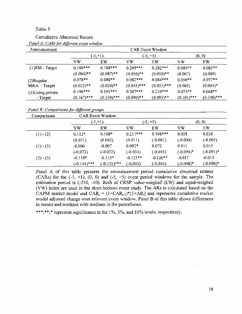
Table 9

Cumulative Abnormal Return Panel A: CARs for different event window Announcement CAR Event Window

(-1,+1) (-5,+5) (0, 0) VW EW VW EW VW EW

(1)RM-Target 0.190*** 0.188*** 0.299*** 0.282*** 0.084** 0.083** (0.094)** (0.087)** (0.056)** (0.050)** (0.007) (0.009)

(2)Regular 0.078** 0.080** 0.082*** 0.084*** 0.056** 0.057** M&A - Target (0.023)** (0.024)** (0.045)*** (0.051)*** (0.003) (0.004)*

(3)Going private 0.196*** 0.195*** 0.207*** 0.210*** 0.073** 0.068** - Target (0.167)** * (0.159)*** (0.090)** (0.095)** (0.101)*** (0.100)***

Panel B: Comparisons for different groups Comparisons CAR Event Window

(-1,+D (-5,+5) (0, 0) VW EW VW EW VW EW

( l ) - ( 2 ) 0.112* 0.108* 0.217*** 0.198*** 0.028 0.026 (0.071) (0.063) (0.011) (-0.001) (-0.004) (-0.005)

( l ) - ( 3 ) -0.006 -0.007 0.092* 0.072 0.011 0.015 (-0.073) (-0.072) (-0.034) (-0.045) (-0.094)* (-0.091)*

(2)-(3) -0.118* -0.115* -0.125** -0.126** -0.017 -0.011 (-0.144)*** (-0.135)*** (-0.045) (-0.044) (-0.098)* (-0.096)*

Panel A of this table presents the announcement period cumulative abnormal returns (CARs) for the (-1, +1), (0, 0) and (-5, +5) event period windows for the sample. The estimation period is (-210, -10). Both of CRSP value-weighed (EW) and equal-weighed (VW) index are used in the short-horizon event study. The ARs is calculated based on the CAPM market model and C A R = ( l+CARj . i )*( l+AR) and represents cumulative market model adjusted change over relevant event window. Panel B of this table shows differences in means and medians with medians in the parentheses.

***,**,* represent significance at the 1%, 5%, and 10% levels, respectively.

38

Table 6 Robustness for Cumulative Abnormal Return

Panel A: CARs for different event window Announcement CAR Event Window

(-U+D (-5, +5) (0, 0) VW EW VW EW VW EW

(l)Reverse 0 291*** 0.189*** 0.318*** 0.316** 0.082** 0.083** Merger - Target (0.008)* (0.007) (0.048)** (0.043)** (0.002)* (0.003)*

(2)Regular 0.079*** 0.076*** 0.076*** 0.073*** 0.056** 0.054** M&A - Target (0.028)** (0.027)* (0.041)** (0.039)** (0.008)* (0.008)*

(3)Going private 0.176*** 0.177*** 0.279*** 0.269*** 0.107** 0.108** - Target (0.145)*** (0.148)*** (0.096)*** (0.098)*** (0.131)*** (0.139)***

Panel B: Comparisons for different groups Comparison CAR Event Window

T-test (-1,+D (-5,+5) (0, 0) (Wilcoxon Z) VW EW VW EW VW EW

( l ) - ( 2 ) 0.112** 0.113** 0.242*** 0.243*** 0.026 0.029 (-0.020) (-0.020) (-0.007) (0.004) (-0.006) (-0.005)

( l ) - ( 3 ) 0.015 0.012 0.039 0.047 -0.025 -0.025 (-0.137)** (-0.141)** (-0.048) (-0.055) (-0.129)** (-0.136)**

(2)-(3) -0.097** -0.101** -0.203** -0.196** -0.051* -0.054* (-0.117)** (-0.121)** (-0.055)* (-0.059)* (-0.123)** (-0.131 )**

Panel A of this table presents the announcement period cumulative abnormal returns (CARs) for the (-1, +1), (0, 0) and (-5, +5) event period windows for the sample. The estimation period is (-210, -10). Both of CRSP value-weighed (EW) and equal-weighed (VW) index are used in the short-horizon event study. The ARs is calculated based on market adjusted abnormal return AR; = R, - Rm and CAR; = (l+CARj_i)*(l+ARj) and represents cumulative market-adjusted change over relevant event window. Panel B of this table shows differences in means and medians with medians in the parentheses..

***,**,* represent significance at the 1%, 5%, and 10% levels, respectively.

39

Table 9

Multivariate regression of 3-day (-1, +1) cumulative abnormal returns

RM - Target M & A - Target G P - Target CAR type EW VW EW VW EW VW Intercept -0.363 -0.430 0.479 0.510 0.435 0.441

(-1.83)** (-1.81)** (3 19)*** (3.76)*** (1.91)** (1.98)** Termination Fee -0.193 -0.221 -0.026 -0.029

(-1.85)** (-2.32)** (-1.12) (-1.22) Deal Value -0.0001 -0.0001 -0.0001 -0.0001 0.001 0.001

(-2.18)** (-3.67)*** (-0.08) (-0.19) (0.12) (0.14) Duration -0.001 -0.001 -0.0009 -0.0009 -0.000 -0.000

(-1.91)** (-1.95)** (-1.81)** (-1.93)** (-0.01) (-0.01) Ownership 1.063 1.079 0.169 -0.172

(4.51)*** (3.72)*** (-0.67) (-0.89) Log(Total Assets) -0.010 -0.011 -0.059 -0.050 -0.000 -0.000

(-0.71) (-0.69) (-2.59)** (-2.67)** (-0.00) (-0.00) ROA -0.181 -0.179 0.123 0.127 -0.014 -0.013

(-1.27) (-1.25) (0.57) (1.13) (-0.22) (-0.20) Cash/Total Assets -0.063 -0.083 0.121 0.116 0.941 0.946

(-0.49) (-0.59) (0.86) (0.93) (2.26)** (2.35)** Debt/Total Assets -0.019 -0.018 0.056 0.043 -0.339 -0.332

(-1.61)* (-1.53)* (1.31)* (1.58)* (-2.10)** (-1.99)**

Adjusted i?-square 0.3750 0.3634 0.1864 0.1986 0.2158 0.2041 F-Statistic 110.90*** 314.60*** 13 97*** 13.68*** 12.97 ** No. of observations 64 64 64 64 64 64

This table shows the multivariate regression results. The dependent variables are the 3-day (-1, +1) announcement period CARs (calculated by using CAPM model) for the sample RM targets and matching counterparts. Variables of deal characteristics in the multivariate regression include: 1) Termination fee which is the amount of the charge on a party who terminates the term of merger transaction in advance of effective date (in million US dollars); 2) Deal Value which is the market value of exchanged stocks in a merger transaction reported in SDC; 3) Duration which is the number of days between announcement date and effective date of the transaction, and 4) Ownership which is the percentage of merged entity's share held by previous private shareholders. T-statistics are reported in parentheses. ****** represent significance at the 1%, 5%, and 10% levels, respectively.

40

Table 9

Post-event return performance - BHRs and BHARs

Period N BHRs BHARs BHARs (in months) RM M&A Mean diff t-statistic

(median) (median) (Median diff) (Wilcoxon Z) 6 64 0.010 0.019 -0.009 -0.32

(0.008) (-0.011) (0.003) (0.13) 12 57 -0.030 -0.018 -0.012 -2.09**

(-0.032) (0.001) (-0.033) (-2.15)** 18 46 -0.045 -0.011 -0.034 -1.73**

(-0.047) (-0.004) (-0.043) (-2.15)** 24 39 -0.036 -0.028 -0.008 -1.86**

(-0.032) (-0.007) (-0.025) (-2.26)** 30 35 -0.081 -0.009 -0.072 -3 97***

(-0.004) (-0.012) (0.008) (2.98)*** 36 31 -0.048 -0.021 -0.027 -2.16**

(-0.038) (-0.008) (-0.03) (-1.76)**

This table shows the equally-weighed Buy-and-hold returns (BHRs) for post-event 6, 12, 18, 24, 30 and 36 month time period. BHRs for RM and matching M&A are reported in this table.

Ti

BHRit = + Rit) - 1 t=2

And the Buy-and-hold abnormal returns (BHARs) are calculated as the difference between RM and its matching M&A.

BHARit = BHRit - BHR]t Where Rit = the return to stock i over day t Ti = end of holding period for stock i j = the matching stock to stock i

T-statistic and Wilcoxon-Z (in parentheses) are reported for BHARs in the last column. ***,**,* represent significance at the 1%, 5%, and 10% levels, respectively.

41

Table 9

Calendar - Time Portfolio Regression

Rpt ~ Rft = a + P{Rmt - R f t ) + sSMBr + hHMLt + spt

Month Coefficient Estimates a b s h Adj. R2

RM -0.0131 0.0073 0.0091 0.0037 0.1003 (-59.31)*** (25.13)*** (21.45)*** (6.37)***

M&A -0.0129 0.0772 0.0096 0.0013 0.1636 (-61.39)*** (27.50)*** (26.01)*** (3.06)***

Comparison -0.0002 -0.0699 -0.0005 0.0024 0.1899 (-2.39)*** (-3.36)*** (-0.88) (1.44)*

RM -0.0188 0.0393 0.0022 -0.0006 0.1475 (-113.54)*** (1.93)** (8.31)*** (-1.62)*

M&A -0.0142 0.0727 0.0089 0.0008 0.2764 (-66.59)*** (26.78)*** (23.48)*** (1.73)**

Comparison -0.0046 -0.0423 -0.0062 -0.0002 0.1713 (-8.19)*** (-0.98) (-4.06)*** (-0.86)

RM -0.0179 0.0486 0.0018 -0.0011 0.2901 (-97.96)*** (2.23)** (5.59)*** (-2.90)***

M&A -0.0141 0.0764 0.0092 -0.0004 0.2159 (-68.57)*** (30.51)*** (25.57)*** (-0.95)

Comparison -0.0028 -0.0215 -0.0079 -0.0009 0.2521 (-18.23)*** (-2.03)** (-1.98)** (-3.36)***

RM -0.0155 0.0783 0.0019 0.0007 0.1983 (-97.66)*** (4.37)*** (7.07)*** (2.00)**

M&A -0.0138 0.0760 0.0090 -0.0009 0.1391 (-69.29)*** (13.81)*** (26.41)*** (-2.19)**

Comparison -0.0017 0.0023 -0.0072 0.0001 0.2144 (-3.87)*** (0.41) (-0.78) (1.26)

42

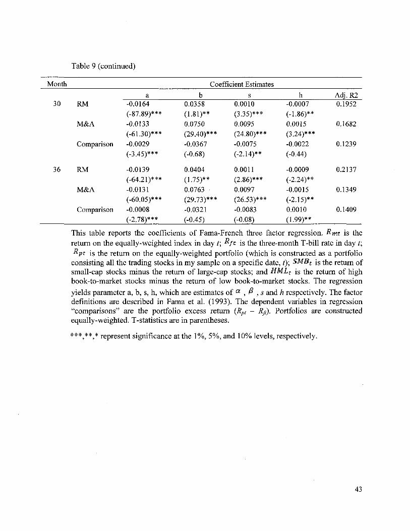
Table 9 (continued)

Month Coefficient Estimates a b s h Adj. R2

30 RM -0.0164 0.0358 0.0010 -0.0007 0.1952 (-87.89)*** (1.81)** (3.35)*** (-1.86)**

M&A -0.0133 0.0750 0.0095 0.0015 0.1682 (-61.30)*** (29.40)*** (24.80)*** (3.24)***

Comparison -0.0029 -0.0367 -0.0075 -0.0022 0.1239 (-3.45)*** (-0.68) (-2.14)** (-0.44)

36 RM -0.0139 0.0404 0.0011 -0.0009 0.2137 (-64.21)*** (1.75)** (2.86)*** (-2.24)**

M&A -0.0131 0.0763 0.0097 -0.0015 0.1349 (-60.05)*** (29.73)*** (26.53)*** (-2.15)**

Comparison -0.0008 -0.0321 -0.0083 0.0010 0.1409 (-2.78)*** (-0.45) (-0.08) (1.99)**

This table reports the coefficients of Fama-French three factor regression. Rmt is the return on the equally-weighted index in day t\ fyt is the three-month T-bill rate in day t\

is the return on the equally-weighted portfolio (which is constructed as a portfolio consisting all the trading stocks in my sample on a specific date, t); SMBt js the return of small-cap stocks minus the return of large-cap stocks; and HMLt i$ the return of high book-to-market stocks minus the return of low book-to-market stocks. The regression

yields parameter a, b, s, h, which are estimates of a , ft , 5 and h respectively. The factor definitions are described in Fama et al. (1993). The dependent variables in regression "comparisons" are the portfolio excess return (Rpt - Rft). Portfolios are constructed equally-weighted. T-statistics are in parentheses.

* * * * * * represent significance at the 1%, 5%, and 10% levels, respectively.

43

Tabl

e 10

Acc

ount

ing

and

oper

atin

g pe

rfor

man

ce o

f pos

t-ev

ent

time

peri

od

Pane

l A

RM (1

) •

M&

A (

2)

(l)v

s. (

2)

Yea

r R

OA

C

ash

Deb

t R

OA

C

ash

Deb

t R

OA

C

ash

Deb

t /a

sset

s /a

sset

s /a

sset

s /a

sset

s /a

sset

s /a

sset

s -1

m

ean

-0.2

13

0.17

6 0.

453

-0.0

57

0.33

1 0.

110

-0.1

6***

-0

.16*

* 0.

34**

* (m

edia

n)

(-0.

500)

(0

.110

) (0

.147

) (0

.010

) (0

.273

) (0

.026

) (-

0.16

)***

(-

0.16

)**

(0.1

2)**

1

mea

n -0

.485

0.

232

0.12

1 -0

.053

0.

253

0.15

7 -0

.61*

**

-0.0

2 -0

.04

(med

ian)

(-

0.11

6)

(0.1

53)

(0.0

24)

(0.0

44)

(0.1

67)

(0.0

33)

(-0.

14)*

* (-

0.01

) (-

0.01

) 2

mea

n -0

.182

0.

233

0.13

0 -0

.051

0.

219

0.08

3 -0

.31*

**

0.01

0.

05

(med

ian)

(-

0.15

5)

(0.0

67)

(0.0

20)

(0.0

17)

(0.1

25)

(0.0

25)

(-0.

18)*

* (-

0.06

) (-

0.01

) -1

vs.

1 T-

test

0.

28**

-0

.06

0.33

**

0.00

0.

06

-0.0

5 (Z

) (-

0.38

)**

(-0.

04)

(0.1

2)*

(-0.

03)

(0.1

1)*

(-0.

01)

1 vs

. 2

T-te

st

-0.3

0**

0.00

-0

.01

0.00

0.

03

0.07

(Z

) (0

.04)

(-

0.09

) (0

.00)

(0

.03)

(0

.04)

(0

.01)

-1

vs.

2 T-

test

-0

.03

-0.0

6 0.

32**

0.

00

0.09

* 0.

02

(Z)

(-0.

35)*

* (0

.04)

(0

.13)

**

(-0.

01)

(0.1

5)**

(0

.00)

Pane

l A

of

this

sho

ws

perf

orm

ance

rat

ios

and

bala

nce

shee

t ch

arac

teri

stic

s. R

OA

, C

ash

to a

sset

s an

d D

ebt

to a

sset

s ar

e ex

amin

ed u

sing

all

activ

e fi

rms

in e

ach

time

peri

od a

nd Y

ear

1 is

fir

st r

epor

ting

cycl

e af

ter

tran

sact

ion

for

one

full

year

, ye

ar 2

is

the

seco

nd r

epor

ting

cycl

e af

ter t

rans

actio

n fo

r one

ful

l yea

r. R

OA

, acc

ount

ing

perf

orm

ance

and

Cas

h/as

sets

and

Deb

t/ass

ets

repr

esen

t bal

ance

she

et c

hara

cter

istic

s.

For

year

-1,

the

RO

As

are

calc

ulat

ed a

s (E

BIT

of

Targ

ets

+ E

BIT

of

Acq

uire

rs)

/ (T

arge

t A

sset

s +

Acq

uire

r A

sset

s).

Lik

ewis

e ca

sh r

atio

an

d de

bt r

atio

are

cal

cula

ted

as (

Cas

h of

Tar

gets

+ C

ash

of A

cqui

rers

) /

(Tar

get

Ass

ets

+ A

cqui

rer

Ass

ets)

and

(D

ebt

of T

arge

ts +

Deb

t of

A

cqui

rers

) / (

Targ

et A

sset

s +

Acq

uire

r A

sset

s), r

espe

ctiv

ely.

M

edia

ns a

re i

n pa

rent

hese

s.

***,

**,*

rep

rese

nt s

igni

fica

nce

at th

e 1%

, 5%

, and

10%

leve

ls,

resp

ectiv

ely.

Pane

l B

RM

(1)

M

&A

(2)

(1

) vs.

(2)

Yea

r R

OA

C

ash

Deb

t R

OA

C

ash

Deb

t R

OA

C

ash

Deb

t /a

sset

s /a

sset

s /a

sset

s /a

sset

s /a

sset

s /a

sset

s -1

m

ean

-0.2

56

0.18

7 0.

616

-0.0

94

0.31

3 0.

095

-0.8

7**

-0.1

3**

0.52

**

(med

ian)

(-

0.01

0)

(0.1

16)

(0.1

56)

(-0.

017)

(0

.226

) (0

.020

) (-

0.17

) (-

0.11

)**

(0.1

4)**

* 1

mea

n -0

.489

0.

235

0.12

3 -0

.055

0.

257

0.15

9 -0

.61*

* -0

.02

-0.0

4 (m

edia

n)

(-0.

116)

(0

.153

) (0

.024

) (0

.044

) (0

.167

) (0

.033

) (-

0.14

)***

(-

0.01

) (-

0.01

) 2

mea

n -0

.182

0.

233

0.13

0 -0

.051

0.

219

0.08

3 -0

.31*

* 0.

01

0.05

(m

edia

n)

(-0.

155)

(0

.067

) (0

.020

) (0

.017

) (0

.125

) (0

.025

) (-

0.18

)***

(-

0.06

) (-

0.01

) -1

vs.

1 T-

test

0.

23**

-0

.50

0.49

**

-0.0

4 0.

06

-0.0

6 (Z

) (0

.11)

* (-

0.04

) (0

.13)

* (-

0.06

) (0

.06)

(-

0.01

) 1

vs. 2

T-

test

-0

.31*

* 0.

00

-0.0

1 0.

00

0.04

0.

08

(Z)

(0.0

4)

(0.0

9)

(0.0

0)

(0.0

3)

(0.0

4)

(0.0

1)

-1 v

s. 2

T-te

st

-0.0

7 -0

.05

0.49

**

-0.0

4 0.

09

0.01

(Z

) (0

.15)

(0

.05)

(0

.14)

**

(-0.

03)

(0.1

0)*

(-0.

01)

Pane

l B

of

this

sho

ws

perf

orm

ance

rat

ios

and

bala

nce

shee

t ch

arac

teri

stic

s. R

OA

, C

ash

to a

sset

s an

d D

ebt t

o as

sets

are

exa

min

ed u

sing

onl

y su

rviv

ing

firm

s in

Yea

r 2.

Yea

r 1

is f

irst

repo

rtin

g cy

cle

afte

r tr

ansa

ctio

n fo

r on

e fu

ll ye

ar,

year

2 i

s th

e se

cond

rep

orti

ng c

ycle

aft

er

tran

sact

ion

for o

ne f

ull y

ear.

RO

A,

acco

unti

ng p

erfo

rman

ce a

nd C

ash/

asse

ts a

nd D

ebt/

asse

ts r

epre

sent

bal

ance

she

et c

hara

cter

istic

s.

For

year

-1,

the

RO

As

are

calc

ulat

ed a

s (E

BIT

of

Targ

ets

+ E

BIT

of

Acq

uire

rs)

/ (T

arge

t A

sset

s +

Acq

uire

r A

sset

s).

Lik

ewis

e ca

sh r

atio

an

d de

bt r

atio

are

cal

cula

ted

as (

Cas

h of

Tar

gets

+ C

ash

of A

cqui

rers

) /

(Tar

get

Ass

ets

+ A

cqui

rer

Ass

ets)

and

(D

ebt

of T

arge

ts +

Deb

t of

A

cqui

rers

) /

(Tar

get

Ass

ets

+ A

cqui

rer

Ass

ets)

, res

pect

ivel

y.

Med

ians

are

in

pare

nthe

ses.

***.

**,*

rep

rese

nt s

igni

fica

nce

at th

e 1%

, 5%

, and

10%

lev

els,

res

pect

ivel

y.

Table 10

Financing activities after RM

Number of firms Number of firms within one year within two year

Public financing 10 28 Bond Issues 0 0

Equity Issues 10 28 Private Financing 14 28

Bond issues only 5 11 Equity issues only 12 20

Bond and Equity issues 3 3 Total Issuances 24 56

This table reports the number of firms that undertook financing activities after reverser merger. The public financing refers to raising fund through public offerings - equity or debt; while the private financing refers to raising fund through individuals or institutions, PIPE financings and other types of private placements.

Appendix A

Description of variables

Variables Description

Total Assets The sum of current and long assets by company

ROA Return on Total assets, defined as earnings before interest and taxes divided by total assets

Termination Fee the amount of the charge on a party who terminates the term of merger transaction in advance of effective date (in million US dollars)

Deal Value The market value of exchanged stocks in a merger transaction reported in SDC

Ownership The portion of shares of the merged entity owned by previous private shareholders

Duration Days between announcement date and effective date of a merger

Liquidity Debt to Total assets

Profitability Cash to Total assets

47