The “Native Fish” Bayesian networks

Ann Nicholson∗ Owen Woodberry† Charles Twardy‡

Bayesian Intelligence Technical Report 2010/3November 18, 2010

Abstract

We present the “Native Fish” Bayesian network, a pedagogical model developed to introduce Bayesiannetworks to ecologists. The network models a hypothetical situation where pesticides are used on cropswhich impact upon the native fish population in a nearby river system. The network is developed incre-mentally. The first basic network, Version 1, contains nodes for Annual Rainfall, Drought Conditions,Tree Condition, Pesticide Use, Pesticide in River, River Flow and Native Fish Abundance. The networkis augmented in Version 2 with nodes for ENSO, Crop Yield and Irrigation. In Versions 1 and 2 the nodesare all discrete and qualitative. In Version 3, the nodes are made continuous then discretised, and theCPTs are generated from equations. In Version 4, we present a decision network, where Pesticide Useand Irrigation become decision nodes, utility nodes are added to represent Landholder Income, Pesticideand Irrigation Costs, as well as the Environmental Value associated with native fish abundance. For eachversion, we show screenshots of the Netica BN software showing the posterior probabilities computedfor a range of predictive and diagnostic reasoning scenarios.

∗Corresponding author. Email: Ann.Nicholson@bayesian-intelligence.com; Tel: +61395431192†Owen.Woodberry@bayesian-intelligence.com‡ctwardy@gmail.com

1

Contents

1 Introduction 3

2 The Initial Model (Version 1) 42.1 The scenario . . . . . . . . . . . . . . . . . . . . . . . . . . . . . . . . . . . . . . . . . . . 42.2 The variables . . . . . . . . . . . . . . . . . . . . . . . . . . . . . . . . . . . . . . . . . . 42.3 Nodes and values . . . . . . . . . . . . . . . . . . . . . . . . . . . . . . . . . . . . . . . . 52.4 Arcs . . . . . . . . . . . . . . . . . . . . . . . . . . . . . . . . . . . . . . . . . . . . . . . 52.5 Assumptions . . . . . . . . . . . . . . . . . . . . . . . . . . . . . . . . . . . . . . . . . . 62.6 Probability Distributions . . . . . . . . . . . . . . . . . . . . . . . . . . . . . . . . . . . . 7

2.6.1 Annual Rainfall . . . . . . . . . . . . . . . . . . . . . . . . . . . . . . . . . . . . . 72.6.2 Pesticide Use . . . . . . . . . . . . . . . . . . . . . . . . . . . . . . . . . . . . . . 82.6.3 Drought Conditions . . . . . . . . . . . . . . . . . . . . . . . . . . . . . . . . . . . 82.6.4 Pesticide in River . . . . . . . . . . . . . . . . . . . . . . . . . . . . . . . . . . . . 92.6.5 River Flow . . . . . . . . . . . . . . . . . . . . . . . . . . . . . . . . . . . . . . . 102.6.6 Tree Condition . . . . . . . . . . . . . . . . . . . . . . . . . . . . . . . . . . . . . 102.6.7 Native Fish Abundance . . . . . . . . . . . . . . . . . . . . . . . . . . . . . . . . . 11

2.7 Inference & Reasoning (using Version 1) . . . . . . . . . . . . . . . . . . . . . . . . . . . . 12

3 Augmented Model (Version 2) 153.1 ENSO . . . . . . . . . . . . . . . . . . . . . . . . . . . . . . . . . . . . . . . . . . . . . . 163.2 Irrigation . . . . . . . . . . . . . . . . . . . . . . . . . . . . . . . . . . . . . . . . . . . . 163.3 Annual Rainfall . . . . . . . . . . . . . . . . . . . . . . . . . . . . . . . . . . . . . . . . . 163.4 River Flow . . . . . . . . . . . . . . . . . . . . . . . . . . . . . . . . . . . . . . . . . . . 173.5 Crop Yield . . . . . . . . . . . . . . . . . . . . . . . . . . . . . . . . . . . . . . . . . . . . 173.6 Inference & Reasoning (using Version 2) . . . . . . . . . . . . . . . . . . . . . . . . . . . . 18

4 Continuous Nodes and Equations (Version 3) 214.1 ENSO . . . . . . . . . . . . . . . . . . . . . . . . . . . . . . . . . . . . . . . . . . . . . . 214.2 Annual Rainfall . . . . . . . . . . . . . . . . . . . . . . . . . . . . . . . . . . . . . . . . . 214.3 River Flow . . . . . . . . . . . . . . . . . . . . . . . . . . . . . . . . . . . . . . . . . . . 214.4 Pesticide Use . . . . . . . . . . . . . . . . . . . . . . . . . . . . . . . . . . . . . . . . . . 224.5 Crop Water . . . . . . . . . . . . . . . . . . . . . . . . . . . . . . . . . . . . . . . . . . . 224.6 Crop Yield . . . . . . . . . . . . . . . . . . . . . . . . . . . . . . . . . . . . . . . . . . . . 224.7 Pesticide in River . . . . . . . . . . . . . . . . . . . . . . . . . . . . . . . . . . . . . . . . 224.8 Native Fish Abundance . . . . . . . . . . . . . . . . . . . . . . . . . . . . . . . . . . . . . 234.9 Inference & Reasoning (using Version 3) . . . . . . . . . . . . . . . . . . . . . . . . . . . . 23

5 Decision Network (Version 4) 255.1 Review . . . . . . . . . . . . . . . . . . . . . . . . . . . . . . . . . . . . . . . . . . . . . 255.2 Adding decision and utility nodes . . . . . . . . . . . . . . . . . . . . . . . . . . . . . . . 255.3 Some sequential decision-making scenarios (Version 4) . . . . . . . . . . . . . . . . . . . . 27

A Versions & Filenames 29

2

1 Introduction

“Native Fish” is a pedagogical model developed to introduce Bayesian networks to ecologists. It is almostas simple as the ubiquitous “Alarm” network [10], and better-suited to the domain, easing the transition tomodeling and elicitation – what we call Knowledge Engineering with Bayesian Networks (KEBN) [5, 15].“Native Fish” is strictly pedagogical. Although it draws on our academic and consulting experience, themodel is vastly simplified for teaching purposes. For more realistic ecological examples, see [12] or somechapters in [13].

Although “Native Fish” is used to help teach Bayesian networks, this report is not a Bayesian networktutorial. It is a reference for the “Native Fish” model, and assumes basic familiarity with Bayesian networks.Readers wishing an introduction to Bayesian networks are encouraged to consult any of [7, 8, 6, 11, 1, 5,3, 4]. Of these, Murphy and Charniak are available online and many people find them useful. Pearl’sintroductory essay is also online, and is very short and very clear.1 Korb & Nicholson, Jensen & Nielsonand Kjærulff & Madsen are all accessible introductory texts, while Neapolitan’s excellent books will appealto the more mathematically-inclined.

As a brief reminder, we provide the following definition.

Definition 1 (Bayesian Network) A Bayesian network is:

1. A directed, acyclic graph, among

2. a set of random variables making up the nodes in the network, with

3. a set of directed links or arrows connecting pairs of nodes from parent to child, where

4. each node has a possibly-stochastic function that quantifies the effects the parents have on the node.

The arcs in a Bayesian network show direct influence. That is:

Definition 2 (X→ Y:) “X has a direct influence on Y”

The nature of that influence may vary. The definition states only that some effect of X on Y remainsno matter what other variables we condition on or control for. Nothing in the mathematical definitionrequires this influence to be causal, but among physically distinct variables, the most natural interpretationis causal, and there is a close correspondence between minimal Bayesian networks and causality. (See forexample, [9, 14].) When the arcs are causal, the Bayesian network can model physical interventions thatbreak previous modeling assumptions, as well as standard observations that do not. Arcs in “Native Fish”are presumed to be causal, unless otherwise stated.

We refer to nodes using a family metaphor.

Definition 3 (Family metaphor:) Arcs go from parent nodes to child nodes.

• Parent⇒ Child

• Ancestor⇒ . . .⇒ Descendant1His books, on the other hand, are more difficult, and are not included in this list.

3

2 The Initial Model (Version 1)

2.1 The scenario

The following paragraph presents the “Native Fish” scenario. Key concepts are highlighted for later refer-ence.

A local river with tree-lined banks is known to contain native fish populations, which needto be conserved. Parts of the river pass through croplands, and parts are susceptible to droughtconditions. Pesticides are known to be used on the crops. Rainfall helps native fish populationsby maintaining water flow, which increases habitat suitability as well as connectivity betweendifferent habitat areas. However rain can also wash pesticides that are dangerous to fish fromthe croplands into the river. There is concern that the trees and native fish will be affected bydrought conditions and crop pesticides.

In short, we want to model the effect of pesticide use and rainfall on native fish abundance and tree condition.

2.2 The variables

We are most concerned about the native fish abundance, but since tree condition is also influenced by thesame factors, it can serve as a proxy variable, or provide additional evidence about hidden factors likepesticide levels in the river itself. Reading the text, we see that native fish abundance and tree condition areboth endpoints: they do not causally affect other variables in the model. Both variables are self-explanatory.

In this model, native fish abundance has two main stressors: water-related and pesticide-related. Themodel also has three variables describing the water-related stressor:

water flow and connectivity: More water keeps the river from fragmenting into ponds, and leads to fasterflow, which washes out pollutants. Higher water levels are better for the fish.

rainfall: This is intended to be year-to-date rainfall, a relatively short-term indicator.

drought conditions: A long-term indicator intended to summarize historical conditions. A multi-yeardrought will leave the soil quite dry, so that rain which falls soaks into the ground before reach-ing the rivers. (For this reason, much of the rain in the Australian reservoir catchment areas has failedto reach the reservoirs.)

Two variables describe the pesticide-related stressor:

Pesticide use: How much pesticide is being used in the river catchment.

Pesticide concentration in river: The amount of pesticide in the river itself – which for this example weimagine cannot easily be directly observed.

For now, we omit other variables such as croplands and habitat suitability, and ENSO, the El NiñoSouthern Oscillation that drives drought cycles in Australia. We also choose to ignore connectivity, summa-rizing its effects in River flow. In an actual model, these decisions should be made on the basis of subjectmatter expertise, desired model fidelity, and time available. Sensitivity analysis can also help decide whichvariables most need to be refined. In this example, we presume that analysis has suggested the current setof variables for the first cycle of model development. Recall that our main goal is pedagogy.

4

Node name Type ValuesNative Fish Abundance Ordered-3 {High, Medium, Low}Tree Condition Ordered-3 {Good, Damaged, Dead}

Ordered-2 {Good, Poor}River Flow Ordered-2 {Good, Poor}

Ordered-3 {High, Medium, Low}Drought Conditions Nominal-2 {Yes, No}Annual Rainfall Ordered-3 {Below average, Average, Above Average}

Continuous {0...50, 51...200, 201...400}Pesticide Use Ordered-2 {High, Low}Pesticide in river Ordered-2 {High, Low}

Table 1: Nodes and possible values for the seven variables in our model. Some variables illustrate alternativevalues.

Node Depends OnNative Fish Abundance River Flow, Pesticide in RiverTree Condition Annual Rainfall, Drought conditionsRiver Flow Annual Rainfall, Drought ConditionsPesticide In River Pesticide Use, Annual RainfallPesticide UseAnnual RainfallDrought Conditions

Table 2: Dependencies in the Native Fish model

2.3 Nodes and values

Having identified our key variables, we then must choose whether they will be continuous, integer, ordered,or nominal. Depending on our software, we may have to discretize continuous or integer variables, so weshould specify likely bins or ranges. For other variables, we have to decide how many states each node has.For ordered variables, that decision may depend on the precision of our knowledge and/or data.

Table 1 sets out the main options for each variable. We use “Ordered-3” to specify an ordered node withthree states, such as {High, Medium, Low}. Nominal nodes have no implied ordering, such as {Red,Green,Blue}. Binary nodes with states like {On, Off}, {True, False}, or {Yes, No} may or may not have an impliedorder. In “Native Fish”we treat such variables as nominal (unordered).

Depending upon the software, the node type can matter for defining, encoding, learning, or doing infer-ence with the probability distribution at the node.

The next step is to specify the structure of model by defining arcs showing which nodes depend on whichother nodes.

2.4 Arcs

Rereading the scenario, we can infer the dependencies in Table 2. Starting from the endpoints, we first decidewhich variables directly influence Native Fish Abundance and Tree Condition (River Flow and Pesticidein River), then decide which variables will directly influence them. These nodes, Pesticide Use, AnnualRainfall, and Drought Conditions do not depend on any of the other variables, so they become “root” nodesin the model. The resulting Version 1 model is shown in Figure 1.

5

Figure 1: Structure of the Native Fish model, v.1. We have expanded two steps "backward" from NativeFish Abundance, and stopped there.

This is a good time to remind ourselves of a bit more terminology. Figure 1 has the nodes labeled as“Root”, “Leaf” or “Intermediate”; this network has two leaf nodes and three root nodes.

Definition 4 (Tree analogy) :

• root nodes have no parents.

• leaf nodes have no children.

• The rest are intermediate nodes.

The root nodes do have other causes outside the model, and later we may wish to expand the modelto include them. For example, ENSO drives Annual Rainfall, and Pesticide Use is likely determined bythe type of crops grown, and the expected pest level, which itself may be determined by past and expectedrainfall. However, all models have to stop somewhere, and Native Fish Version 1 stops two levels “back”from Native Fish Abundance. This model also reflects many assumptions which may not be true.

2.5 Assumptions

There is little doubt about the included arcs. As usual, the more controversial assumptions involve themissing arcs. While it is almost certainly true that Pesticide Use does not affect River Flow, the modelmakes the following more dubious assertions:

Pesticides don’t affect tree condition: Pesticides are generally considered harmless to plants, but appar-ently under some conditions, prolonged exposure to pesticides can stunt growth or cause other prob-lems – a condition known as phytotoxicity. The effects are heightened by heat or drought, and it maybe the inactive ingredients and their byproducts that are most phytotoxic.2 Also, if pesticides affectkey pollinators, the trees will have trouble propagating. We assume these are second-order effects andcan be ignored in Version 1.

2http://wihort.uwex.edu/flowers/Phytotoxicity.htm

6

Rainfall and Drought are unrelated: This is patently false. Even using our intended division into short-term and long-term, Drought is a function of recent Rainfall. Furthermore, since Australian droughtscome in extended cycles, being in Drought forecasts low Annual Rainfall. However, the upshot is thatthey provide information about each other, not that their affect on downstream variables is changed.So long as both variables are always observed, downstream predictions will be unaffected by themissing arc. It might even be worthwhile testing whether one of them could be omitted entirely.

Pesticide Use is unrelated to Rainfall or Drought: Pesticides are applied in response to pests. Desertspecies are adapted to wait out long dry spells, and pests may “bloom” in rainy years, introducinga correlation. Conversely, farmers wishing not to stress their plants may apply pesticides more spar-ingly in drought years. But again, if Pesticide Use and Annual Rainfall are both known, the modelimplies their correlation does not matter for pesticide levels in the river.

Other Causes: The effects of all parents not explicitly modeled are summarized the uncertainty in thechild distribution when all parents are known. Therefore it makes sense to include the most importantvariables first. Implicitly, this model asserts that no other causes of Native Fish Abundance are asimportant as Pesticide in River or River Flow. Likewise, that no other causes of Tree Condition are asimportant as Rainfall and Drought.

Both laziness and ignorance are in operation here. Again, the goal was to produce a plausible first-ordermodel for pedagogical purposes. Since part of the goal is to teach the modeling process, all the caveatsnoted above are grounds for subsequent revisions of the model during later tutorial sessions.

2.6 Probability Distributions

The structure shows which variables depend on which other variables, but does not quantify the effect. So,E = mc2 would become m→E←c, which is precisely equivalent to E = f(m, c), a bare statement ofdependence. Each node needs an expression giving its value or distribution as a function of its parents (ifany).

It is customary to call these local functions Conditional Probability Tables, or CPTs. However, in generalthey need not be conditional, probabilistic, or tables. Perhaps the most general term is expressions. When thenode has parents, the expressions are conditional. When there is uncertainty, it is a probability distribution.If we allow that distributions can be degenerate, then all these expressions are probability distributions, andfor intermediate or leaf nodes, they are conditional probability distributions (CPDs). If we wish to callattention to the fact that a distribution is degenerate, we may refer to it as a function if it depends on othernodes, or a default value (for constants).

We begin with distributions for the root nodes, as these are the simplest. Because they give the distribu-tion prior to observing any other values, these are prior probabilities.

2.6.1 Annual Rainfall

In Version 1, we judge rainfall relative to an Average year, and start with a prior belief that most years areAverage.

P(Rainfall = Below Average) 0.1P(Rainfall = Average) 0.7P(Rainfall = Above Average) 0.2

7

To match the format of the CPTs shown below, this table can also be written as follows:

P(Rainfall)Above Average Average Below Average

0.1 0.7 0.2

But in addition to being imprecise, this suffers from vagueness. Over what period is “Average” defined?This node really ought to be a numeric variable measured in mm/yr.3 We will revisit this in a later sectionon making variables continuous.

2.6.2 Pesticide Use

We presume pesticide use.

P(Pesticide Use)High Low0.9 0.1

Subsequent version should replace this with a measure, such as percentage of farms in the catchmentusing pesticides, the frequency of pesticide application, or the total level of pesticide use in the catchment.

2.6.3 Drought Conditions

Consider the following information about rainfall and drought, from the Australian Bureau of Meteorology.Although the Bureau does not declare drought, it does provide state governments with data about rainfall

deficiencies, which inform declarations of drought. The Bureau defines serious and severe deficienciesstatistically:

Serious rainfall deficiency: rainfall over three months (or more) lies between the fifth and tenth percentile.

Severe rainfall deficiency: rainfall over three months (or more) is below the fifth percentile.

By definition, serious deficiencies should occur less than 10% of the time, and severe ones less than 5% ofthe time.4

In the page “Living with Drought”5, the Bureau provides a definition of drought relative to normal wateruse:

Definition 5 (Drought:) A drought is a prolonged, abnormally dry period when there is not enough waterfor users’ normal needs. Drought is not simply low rainfall; if it was, much of inland Australia would be inalmost perpetual drought.

The same page notes that over the long term, Australia has “about three good years and three bad years outof ten,” with intervals between severe droughts varying between 4 and 38 years. Figure 2 shows what theBureau considers to be “Major Australian Drought Years” – presumably ones that affected large portions ofthe country or economy. It’s worth nothing that many regional droughts do not appear in this figure. Alltold, about 30 of the 130 years in the figure are drought years, which is about 25%. We use this as the priorfor our Drought node.

3In earlier versions, the first iteration of the Native Fish model had Annual Rainfall as a discrete node with values.4http://www.bom.gov.au/climate/glossary/drought.shtml5http://www.bom.gov.au/climate/drought/livedrought.shtml

8

Figure 2: Severe national droughts in Australia.

Figure 3: Annual Rainfall at the Melbourne Regional Office, 1855-2010. From the Australian Bureau ofMeteorology Climate Data Online website.

P(Drought)Yes No0.25 0.75

Actual data is available for most places in Australia, sometimes quite far back. Figure 3 shows theaverage rainfall in Melbourne from 1855 to 2010, as recorded by the Melbourne Regional Office station.The tenth percentile for that coastal station is 466mm.6 But it is unlikely one can use data from a singlestation to understand drought. Examining this single dataset shows only four years with three or moreconsecutive months of rainfall below the tenth percentile, but the region was declared to be in serious orsevere deficiency more often than that.

2.6.4 Pesticide in River

The variable “Pesticide in River” represents the pesticide concentration in the river and thus depends onPesticide Use and Annual Rainfall.

6Australian BOM Climate Data Online, Product Code: IDCJAC0001

9

P(PesticideInRiver |PesticideUse, Rainfall)

Pesticide Annual High LowUse RainfallHigh Below Avg 0.3 0.7High Average 0.6 0.4High Above Avg 0.8 0.2Low Below Avg 0.1 0.9Low Average 0.2 0.8Low Above Avg 0.3 0.7

2.6.5 River Flow

River flow is a function of Drought Conditions and Annual Rainfall. Ideally it would be replaced by actualmeasurement of flow, but is currently qualitative. When there is above average rainfall and no drought, weassign a 99% chance of good flow. Conversely, we assign only a 5% chance of good flow if there is belowaverage rainfall and drought. The remaining uncertainty has to cover what is meant by “drought” and “belowaverage” as well as uncertainties in how rainfall and drought affect river flow. Values in other conditionsinterpolate intuitively. The actual values chosen suggest that rainfall dominates: good flow is twice as likelywhen there is drought and above-average rainfall as when there is no drought but below-average rainfall.

P(RiverFlow |Drought, Rainfall)

Drought Annual Good PoorConditions RainfallYes Below Avg 0.05 0.95Yes Average 0.15 0.85Yes Above Avg 0.80 0.20No Below Avg 0.40 0.60No Average 0.60 0.40No Above Avg 0.99 0.01

2.6.6 Tree Condition

The first of our leaf nodes, Tree Condition or “TreeCond” could be interpreted to mean the expected dis-tribution of Good, Damaged, and Dead trees. When conditions are good, we expect only 1% of the treesto be dead, but when they are bad, we expect as much as 20% of them to die. During drought conditions,we expect 60% to show some damage as a result of the overall bad conditions; the current annual rainfallmakes a different, with more dead and fewer in good condition when it is below average. When there arenon-drought conditions, the tree condition improves overall, with the number of damaged ranging from 25%when annual rainfall is below average, down to about 9% when is it above average.

10

P(TreeCond |Drought, Rainfall)

Drought Annual Good Damaged DeadConditions RainfallYes Below Avg 0.20 0.60 0.20Yes Average 0.25 0.60 0.15Yes Above avg 0.30 0.60 0.10No Below Avg 0.70 0.25 0.05No Average 0.80 0.18 0.02No Above Avg 0.90 0.09 0.01

2.6.7 Native Fish Abundance

Native Fish Abundance, also called “FishAbundance” is given as a distribution over High, Medium,and Low abundances. It depends on Pesticide in River and River Flow. In good conditions – low pesticideconcentrations and good flow – a low abundance is unlikely, judged to be about 1 in 20. Low abundance isparticularly sensitive to river flow, and when river flow is poor it jumps to 80-89%. In good conditions, weexpect High abundance 80% of the time. High abundance requires everything to go well, so its probabilitydrops very quickly as conditions deteriorate.

P(FishAbundance |PesticideInRiver, RiverFlow)

Pesticide River High Medium Lowin River FlowHigh Good 0.2 0.4 0.4High Poor 0.01 0.1 0.89Low Good 0.8 0.15 0.05Low Poor 0.05 0.15 0.8

11

2.7 Inference & Reasoning (using Version 1)

In this section we look at the posterior probabilities computed given different scenarios, entered as evidenceinto the BN (shown in Figures 4 & 5).

Fig 4(a): Before observing any evidence, there is already a nearly 52% chance that Native Fish Abundancewill be Low.

Fig 4(b): If we observe a lot of dead trees, the chance rises to 65%. The dead trees raise the probabilityof drought (by diagnostic reasoning from symptom to cause) and the greater probability of droughtraises the chance of poor river flow, raising the chance of low fish abundance.

Fig 4(c): Here, we confirm low fish abundance by observation, further increasing our belief in poor flowcaused by drought. Both observations lower the chance of above average rainfall.

Fig 4(d): This figure shows a predictive reasoning scenario. Rainfall is set to Above Average, almostdoubling the chance of good flow, but also substantially raising the chance of washing pesticide intothe river. The chance of low fish abundance drops from 52% to 34%.

Fig 5(e): If we also observe that there is no long-term drought, we are virtually assured of good flow andgood tree conditions. Probability of low fish abundance drops slightly, still affected by the 3:1 oddsfavoring high pesticide levels.

Fig 5(f): If, as expected, pesticide use is high, then the chance of pesticide in the river rises to 80%, and weare nearly in full ignorance of the native fish abundance.

Fig 5(g): After observing a medium level of native fish abundance, we conclude that pesticide levels in theriver were very likely (91%) high, and that river flow was almost certainly (99.7%) good.

Fig 5(h): Clearing observations and observing only that native fish were in high abundance this year, weexpect good flow and low pesticide levels. The good river flow somewhat increases the chance ofabove-average rainfall, and the net effect is that drought conditions are much less likely (down from25% to 12.5%).

12

(a) No evidence (b) Diagnostic reasoning with worst case TreeCondition

(c) Diagnostic reasoning with worst case Tree (d) Predictive reasoning with best case AnnualCondition and Native Fish Abundance Rainfall

Figure 4: Native Fish BN (Version 1): Reasoning scenarios

13

(e) Predictive reasoning with best case Annual (f) Predictive reasoning with best case AnnualRainfall and Drought Condition Rainfall and Drought Condition, High Pesticide

Use

(g) Mixed reasoning with best case Annual (h) Diagnostic reasoning with best case NativeRainfall and Drought Condition, High Pesticide Fish Abundance

Use and Medium Native Fish Abundance

Figure 5: Native Fish BN (Version 1): Reasoning scenarios (cont.)

14

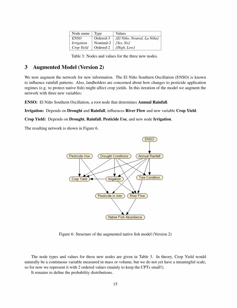
Node name Type ValuesENSO Ordered-3 {El Niño, Neutral, La Niña}Irrigation Nominal-2 {Yes, No}Crop Yield Ordered-2 {High, Low}

Table 3: Nodes and values for the three new nodes.

3 Augmented Model (Version 2)

We now augment the network for new information. The El Niño Southern Oscillation (ENSO) is knownto influence rainfall patterns. Also, landholders are concerned about how changes to pesticide applicationregimes (e.g. to protect native fish) might affect crop yields. In this iteration of the model we augment thenetwork with three new variables:

ENSO: El Niño Southern Oscillation, a root node that determines Annual Rainfall.

Irrigation: Depends on Drought and Rainfall, influences River Flow and new variable Crop Yield.

Crop Yield: Depends on Drought, Rainfall, Pesticide Use, and new node Irrigation.

The resulting network is shown in Figure 6.

Figure 6: Structure of the augmented native fish model (Version 2)

The node types and values for these new nodes are given in Table 3. In theory, Crop Yield wouldnaturally be a continuous variable measured in mass or volume, but we do not yet have a meaningful scale,so for now we represent it with 2 ordered values (mainly to keep the CPTs small!).

It remains to define the probability distributions.

15

3.1 ENSO

There were 23 El Niño events and 19 La Niña events in the twentieth century. While this suggests a prior of[23, 58, 19], we “round off” to take an initial distribution for ENSO as:

P(ENSO)El Niño Neutral La Niña

0.20 0.60 0.20

3.2 Irrigation

The Irrigation variable represents water diverted from the river to the crops. If the focus of study was onthis particular aspect, an improvement could be to split the Irrigation variable into two, one representing theamount taken from the river, and the other, the amount delivered to the crops — as this would not be equal.

P(Irrigation|Drought, Rainfall)

Drought Rainfall Yes NoYes Below average 0.01 0.99Yes Average 0.1 0.9Yes Above average 0.25 0.75No Below average 0.95 0.05No Average 0.5 0.5No Above average 0.2 0.8

Subsequent tables will be easier to show with a screenshot. For comparison, the Netica screenshot7 forIrrigation is:

3.3 Annual Rainfall

The ENSO variable gives new conditionals on the annual rainfall. The following screenshot shows the newtable.

7Netica BN software, www.norsys.com

16

3.4 River Flow

Irrigation takes water out of the river, reducing flow. Therefore, the distribution in River Flow has to dependon Irrigation. River flow is better without irrigation. For a first cut, we imagine that irrigation increases thechance of Poor river flow by around 10%.

The following screenshot shows the modified table. Alternate rows show the expected probability dis-tributions for River Flow, with and without Irrigation.

3.5 Crop Yield

The new variable Crop Yield has two states and four parents. Ideal conditions give a 99% chance of Highyield, declining towards 1% as conditions worsen, with the following progression:

[99, 95, 95, 80, 80, 70, 60, 60, 50, 50, 50, 40, 30, 30, 30, 25, 20, 20, 15, 15, 10, 5, 2, 1]

The full distribution is shown in the following screenshot:

17

3.6 Inference & Reasoning (using Version 2)

In this section we look at the posterior probabilities, of the new nodes, computed given different scenarios,entered as evidence into the BN (shown in Figures 7 & 8).

Fig 7(a): Before observing any evidence, there is already a 55% chance that Crop Yield will be high.

Fig 7(b): If we observe an El Nino event, our probability of below average rainfall increases, and thusreduce the chance of a good crop yield from 55% to 43%.

Fig 7(c): On the other hand, if we observe an La Nina event, the chances of a good crop yield increase to74%.

Fig 7(d): Next we repeat the last two scenarios whist observing Drought Conditions. During a El Ninoevent, drought conditions dramatically reduce the chances of Irrigation, from 61% to 5%.

Fig 8(e): During a La Nina event, drought conditions still reduces the chances of Irrigation, but not sogreatly (29% to 20%).

Fig 8(f): When there is no drought and rainfall is above average, a high crop yield is very likely (94%).

Fig 8(g): From the above scenario, if we observe a low crop yield, we conclude the explanation that thechances of Pesticide Use and Irrigation are low.

18

Fig 8(h): Clearing observations and observing only that crop yield is good, we expect a neutral ENSO(57%) or a La Nina event (27%), and no drought (91%). Additionally it increases the chances thatpesticide and Irrigation have been used.

(a) No evidence (b) Predictive reasoning with El Nino event

(c) Predictive reasoning with La Nina event (d) Predictive reasoning with worst case ENSOand Drought Conditions

Figure 7: Native Fish BN (Version 2): Reasoning scenarios

19

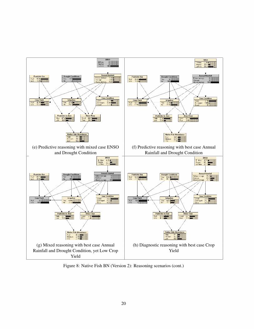
(e) Predictive reasoning with mixed case ENSO (f) Predictive reasoning with best case Annualand Drought Condition Rainfall and Drought Condition

(g) Mixed reasoning with best case Annual (h) Diagnostic reasoning with best case CropRainfall and Drought Condition, yet Low Crop Yield

Yield

Figure 8: Native Fish BN (Version 2): Reasoning scenarios (cont.)

20

4 Continuous Nodes and Equations (Version 3)

As noted earlier, some of our nodes are really continuous variables, and should be defined that way, evenif they have to be discretized for inference. Additionally, some of the tables are getting large and ad-hoc.The relationships are much simpler than a full table would imply. Using equations can help capture the“local” structure. Thus, in this iteration, we convert many nodes to continuous nodes, and, where possible,use equations to describe relationships between nodes. (In Netica, the continous nodes are discretised andthe equations are used to generate the CPTs.)

The changes serve purely as a teaching example. The actual equations and values would withstand evenless scrutiny than the previous version of the network.

There are ten variables in the extended network. At least half are naturally continuous, and two moreare cast as continuous to aid with the equations defining their children. Only Drought, Irrigation, and TreeCondition will remain discrete.

4.1 ENSO

Although there are weak and strong El Niño events, ENSO is naturally a discrete variable. However, sinceAnnual Rainfall is naturally continuous (mm/yr), it will be convenient to define Rainfall as multiples ofENSO. That means ENSO has no units, and an arbitrary scale – we can adjust the constant in the equationfor Rainfall to yield sensible values in mm/yr. We modeled ENSO as a discrete variable with values with anarbitrary scale from -2 to 2. El Nino gets the value -2, Neutral 0 and La Nina 2.

4.2 Annual Rainfall

Annual rainfall is now defined by a normal distribution with mean 126 + 50×ENSO, and a standard devia-tion of 30; the unit is millimetres (mm).

P(Rainfall | ENSO) = NormalDist(Rainfall, 126 + 50*ENSO, 30)

Discretization is [0, 51, 201, 400] for Below average, Average, and Above average.

4.3 River Flow

River Flow is given by a Normal distribution with a mean dependent on Drought and Irrigation, and a fixedstandard deviation of 50. Denote Annual Rainfall by R. Then, in table form:

Drought Irrigation Mean River FlowYes Yes R/3Yes No R/2No Yes R/2No No R

The Netica equation uses the ternary ?: operator for if..then..else:

21

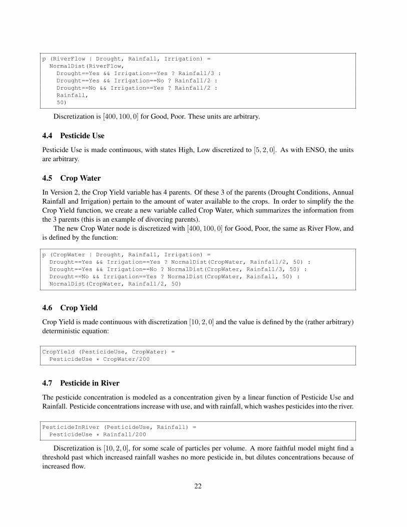
p (RiverFlow | Drought, Rainfall, Irrigation) =NormalDist(RiverFlow,

Drought==Yes && Irrigation==Yes ? Rainfall/3 :Drought==Yes && Irrigation==No ? Rainfall/2 :Drought==No && Irrigation==Yes ? Rainfall/2 :Rainfall,50)

Discretization is [400, 100, 0] for Good, Poor. These units are arbitrary.

4.4 Pesticide Use

Pesticide Use is made continuous, with states High, Low discretized to [5, 2, 0]. As with ENSO, the unitsare arbitrary.

4.5 Crop Water

In Version 2, the Crop Yield variable has 4 parents. Of these 3 of the parents (Drought Conditions, AnnualRainfall and Irrigation) pertain to the amount of water available to the crops. In order to simplify the theCrop Yield function, we create a new variable called Crop Water, which summarizes the information fromthe 3 parents (this is an example of divorcing parents).

The new Crop Water node is discretized with [400, 100, 0] for Good, Poor, the same as River Flow, andis defined by the function:

p (CropWater | Drought, Rainfall, Irrigation) =Drought==Yes && Irrigation==Yes ? NormalDist(CropWater, Rainfall/2, 50) :Drought==Yes && Irrigation==No ? NormalDist(CropWater, Rainfall/3, 50) :Drought==No && Irrigation==Yes ? NormalDist(CropWater, Rainfall, 50) :NormalDist(CropWater, Rainfall/2, 50)

4.6 Crop Yield

Crop Yield is made continuous with discretization [10, 2, 0] and the value is defined by the (rather arbitrary)deterministic equation:

CropYield (PesticideUse, CropWater) =PesticideUse * CropWater/200

4.7 Pesticide in River

The pesticide concentration is modeled as a concentration given by a linear function of Pesticide Use andRainfall. Pesticide concentrations increase with use, and with rainfall, which washes pesticides into the river.

PesticideInRiver (PesticideUse, Rainfall) =PesticideUse * Rainfall/200

Discretization is [10, 2, 0], for some scale of particles per volume. A more faithful model might find athreshold past which increased rainfall washes no more pesticide in, but dilutes concentrations because ofincreased flow.

22

4.8 Native Fish Abundance

Abundance is given by a normal distribution with mean dependent on flow and pesticide concentration lev-els. The equation makes use of Netica’s ternary ?: operator for if..then..else. If concentrations are< 2 (their lowest level), then abundance is half of River Flow, else it is one third River Flow.

p (NativeFish | PesticideInRiver, RiverFlow) =PesticideInRiver<2

? NormalDist(NativeFish, RiverFlow/2, 20): NormalDist(NativeFish, RiverFlow/3, 20)

4.9 Inference & Reasoning (using Version 3)

In this section we look at the posterior probabilities computed given different scenarios, entered as evidenceinto the BN (shown in Figure 9).

Fig 9(a): Before observing any evidence, there is already a 51% chance that Native Fish Abundance willbe low, similar to the previous versions.

Fig 9(b): Next we observe the worst case scenario for the Native Fish Abundance with an El Nino eventand high Pesticide Use. The chances of high Pesticide in the river decreases, because there is lessrunoff, however, the chances of poor River Flow greatly increases resulting in a overall increase in theprobability of low Native Fish Abundance.

Fig 9(c): Clearing the observations and observing a high Native Fish Abundance and good Tree Condition,increases the chances of a La Nina event, No Drought Conditions and low Pesticide Use.

Fig 9(d): Next we change the Native Fish Abundance observation from high to low. This increases thechances of an El Nino event, Drought Conditions and Pesticide Use, however the greatest change is inthe chances of Irrigation, increasing from 27% to 62%, which would explain the low Fish Abundancedespite the good Tree Condition.

23

(a) No evidence (b) Predictive reasoning with worst case ENSOand High Pesticide Use

(c) Diagnostic reasoning with best case Tree (d) Diagnostic reasoning with mixed case TreeCondition and Native Fish Abundance Condition and Native Fish Abundance

Figure 9: Native Fish BN (Version 3): Reasoning scenarios

24

5 Decision Network (Version 4)

Suppose there is a proposal to allow farmers to take water from the river system to irrigate their crops.Increased irrigation will help the crops, but reduce river flows, affecting fish habitat and pesticide concen-trations in the river. Irrigation could increase pesticide runoff.

River managers are looking at the trade-offs in varying the use of fertilisers in the area, and releasingwater for farming irrigation. They want to find the best trade-off. This is a decision problem, and the rightway to model it is by making Irrigation a decision node. For that to work, we have to define utilities. Whenwe augment a Bayesian network with utility and decision nodes, we have a Bayesian decision network,sometimes called an Influence Diagram [2].

5.1 Review

The expected utility of a decision is the probability-weighted value of the decision’s outcomes. The Bayesianoptimal decision is the one with the greatest expected utility.

Definition 6 (Bayesian Optimal Decision) The Bayesian optimal decision maximizes expected utility, wherethe expected utility of a decision is:

E(decision) =∑

i

P (outcomei|decision)× U(outcomei)

Sometimes other optimizations are appropriate. For example, game theory often employs minimax,where each player minimize the maximum loss. However, we restrict ourselves to Bayesian optimal deci-sions, which can be solved entirely within a Bayesian decision network.

5.2 Adding decision and utility nodes

We take as our starting point the augmented discrete network with ENSO, Crop Yield, and Irrigation (Ver-sion 2). To convert this to a decision network, we will define new decision nodes, Pesticide Use and Irriga-tion, and associated utility nodes.

In this simple model, the following utilities suggest themselves:

• Environmental value of Native Fish Abundance

• Landholder Income from Crop Yield

• Pesticide Cost for applying pesticides

• Irrigation Cost from irrigating

They are configured as shown in Figure 10. For demonstration purposes, we have selected rather arbitraryutilities as follows:

Utility Node States UtilitiesEnvironmental Value [High, Medium, Low] [200, 200, -200]Crop Yield [High, Low] [1200, 100]Pesticide Cost [High, Low] [-100, 0]Irrigation Cost [Yes, No] [-200, 0]

25

Figure 10: Decision Network (Version 4) with two decision nodes, Pesticide Use and Irrigation.

Inspection of the table shows that Crop Yield has a strong influence. However, the numbers have beenselected so that before any observations are made, the utilities are only slightly in favor of high pesticide use(512:506). 8

8Utilities have no absolute zero nor a natural scale, so differences and ratios have no metric value. But we may conclude that631:566 is a stronger preference than 358:351.

26

5.3 Some sequential decision-making scenarios (Version 4)

We now look at just a few of the decision scenarios modeled in the Native Fish decision network (shown inFigures 11 & 12):

Fig 11(a-b): Without any observed evidence, the utilities are slightly in favor of High Pesticide Use (512:506).After deciding to use Pesticide, we now see that the utilities also favor Irrigation (512:477).

Fig 11(c-d): Considering the optimal conditions of no drought and a La Nina event, the utilities still favorthe use of pesticides (935:908). However the plentiful crop water supply means that the utility ofIrrigating (given pesticide has been used) is now not in favor (830:935).

(a) No Evidence (b) Utilities favor High Pesticide Use andIrrigation

(c) Best case scenario with La Nina event and (d) Utilities favor High Pesticide Use andNo Drought Conditions No Irrigation

Figure 11: Native Fish Decision network (Version 4): Decision scenarios

27

Fig 12(e-f): Going to the opposite extreme, with drought conditions and an El Nino event, Pesticide useand Irrigation are no longer favored (-13:63 & 29:63), as the payoff on Crop Yield will likely be low,regardless, and will not justify the costs.

Fig 12(g-h): However, when there is no drought, Irrigation is more effective and thus is favored during anEl Nino event (419:364).

(e) Worst case scenario with El Nino event and (f) Utilities favor Low Pesticide Use andDrought Conditions No Irrigation

(g) Mixed case scenario with El Nino Event and (h) Utilities favor Low Pesticide Use andNo Drought Condition Irrigation

Figure 12: Native Fish Decision network (Version 4): Decision scenarios (cont.)

28

A Versions & FilenamesFilename DescriptionNF_V1 Original 7-variable discrete network.NF_V2 Adds 3 variables to NF_V1: ENSO, Irrigation, and Crop

Yield.NF_V3 NF_V2 with 7 variables continuous (all but Drought, Ir-

rigation, and Tree Condition). 4 use equations: Rainfall,Pesticide in River, RiverFlow, and Abundance.

NF_V4 NF_V2with Pesticide Use and Irrigation converted to de-cision nodes. Four utilities nodes added: Pesticide Cost,Irrigation Cost, Landholder Income, EnvironmentalValue.

29

References

[1] Eugene Charniak. Bayesian networks without tears. AI Magazine, pages 50–63, Winter 1991. PDFfile from aaai.org.

[2] R.A. Howard and J.E. Matheson. Influence diagrams. In R.A. Howard and J.E. Matheson, editors,Readings in Decision Analysis, pages 763–771. Strategic Decisions Group, Menlo Park, CA, 1981.

[3] Finn V. Jensen and Thomas D. Nielsen. Bayesian networks and decision graphs. Springer Verlag,New York, 2nd edition, 2007.

[4] Uffe B. Kjærulff and Anders L. Madsen. Bayesian networks and Influence Diagrams: A guide toconstruction and analysis. Springer Verlag, 2008.

[5] Kevin B. Korb and Ann E. Nicholson. Bayesian Artificial intelligence. Chapman & Hall/CRC, 2ndedition, 2010.

[6] Kevin P. Murphy. An introduction to graphical models. Manuscript available on the web, 10 May2001.

[7] Richard E. Neapolitan. Probabilistic Reasoning in Expert Systems. Wiley & Sons, Inc., 1990.

[8] Richard E. Neapolitan. Learning Bayesian Networks. Pearson Prentice Hall, 2004.

[9] J. Pearl. Causality: models, reasoning and inference. Cambridge University Press, New York, 2000.

[10] Judea Pearl. Probabilistic Reasoning in Intelligent Systems. Morgan Kaufmann, San Mateo, CA, 1988.

[11] Judea Pearl. Bayesian networks, causal inference, and knowledge discovery. Second Moment, March2001. Electronic journal.

[12] Carmel A. Pollino, Owen Woodberry, Ann Nicholson, Kevin Korb, and Barry T. Hart. Parameteri-sation and evaluation of a bayesian network for use in an ecological risk assessment. EnvironmentalModelling & Software, 22(8):1140 – 1152, 2007. Bayesian networks in water resource modelling andmanagement.

[13] Olivier Pourret, Patrick Naïm, and Bruce Marcot. Bayesian Networks: A Practical Guide to Appli-cations. Wiley, May 2008.

[14] Charles R. Twardy and Kevin B. Korb. A criterion of probabilistic causality. Philosophy of Science, inpress, 2004.

[15] Charles R. Twardy, Ann E. Nicholson, Kevin B. Korb, and John McNeil. Epidemiological data miningof cardiovascular bayesian networks. electronic Journal of Health Informatics, 1(1), 2006. Inauguralissue; Special issue on health data mining.

30