the money view versus the credit view sarah s. baker ... · sarah s. baker, david l opez-salido,...

Finance and Economics Discussion SeriesDivisions of Research & Statistics and Monetary Affairs

Federal Reserve Board, Washington, D.C.

The Money View Versus the Credit View

Sarah S. Baker, David Lopez-Salido, and Edward Nelson

2018-042

Please cite this paper as:Baker, Sarah S., David Lopez-Salido, and Edward Nelson (2018). “The Money View Versusthe Credit View,” Finance and Economics Discussion Series 2018-042. Washington: Boardof Governors of the Federal Reserve System, https://doi.org/10.17016/FEDS.2018.042.

NOTE: Staff working papers in the Finance and Economics Discussion Series (FEDS) are preliminarymaterials circulated to stimulate discussion and critical comment. The analysis and conclusions set forthare those of the authors and do not indicate concurrence by other members of the research staff or theBoard of Governors. References in publications to the Finance and Economics Discussion Series (other thanacknowledgement) should be cleared with the author(s) to protect the tentative character of these papers.

The Money View Versus the Credit View:

A Comment on Schularick and Taylor, “Credit Booms Gone

Bust: Monetary Policy, Leverage Cycles, and Financial Crises,

1870–2008”

Sarah S. Baker, David Lopez-Salido, and Edward Nelson∗†

July 2, 2018

Abstract

We argue that Schularick and Taylor’s (2012) comparison of credit growthand monetary growth as financial-crisis predictors does not necessarily providea valid basis for achieving one of their stated intentions: evaluating the relativemerits of the “money view” and “credit view” as accounts of macroeconomicoutcomes. Our own analysis of the postwar evidence suggests that money out-performs credit in predicting economic downturns in the 14 countries in Schu-larick and Taylor’s dataset. This contrasts with Schularick and Taylor’s (2012)highly negative verdict on the money view. In accounting for the difference infindings, we first explain that Schularick and Taylor’s characterization of themoney view is defective, both because their criterion for its validity (that rapidmonetary growth predicts financial crises) is misplaced, and because they incor-rectly take the money view’s proponents as relying on the notion that monetaryaggregates are a good proxy for credit aggregates. In fact, the money viewof Friedman and Schwartz does not predict an automatic relationship betweenrapid monetary growth and (financial or economic) downturns, nor does it reston money being a good proxy for credit. We further show that Schularick andTaylor’s data on money have systematic faults. For our reexamination of theevidence, we have constructed new, and more reliable, annual data on moneyfor the countries studied by Schularick and Taylor.

JEL Classification: E32; E51Keywords: money view, credit view, recessions, financial crises.

∗Baker: Federal Reserve Board, [email protected]. Lopez-Salido: Federal Reserve Board,[email protected]. Nelson: Federal Reserve Board, [email protected]. We are grateful toMoritz Schularick and Alan Taylor for helpful comments on an earlier version of this paper. We also havebenefited from advice from numerous colleagues on the collection of monetary data, as detailed in theacknowledgments in Appendix B below.†The views expressed here are the authors’ alone and should not be interpreted as those of the Federal

Reserve or the Board of Governors.

1 Introduction

In an important study, Schularick and Taylor (2012, p. 1030) have investigated “the dy-namics of money, credit, and output across a broad sample of countries over the long run.”A key part of their analysis is the focus of this comment.

Schularick and Taylor (2012, pp. 1030, 1035) juxtapose what they call the “money view”associated with “canonical monetarists like Friedman and Schwartz (1963)”—in which mon-etary aggregates are important for understanding macroeconomic fluctuations—with the“credit view,” which emphasizes the significance of movements in credit aggregates (in par-ticular, aggregate commercial bank loans) for the economy.1 In order to test the merits ofthe two views, they conduct a logit regression analysis, using a dataset they constructedof annual observations for 14 countries. In the regressions, distributed lags of a creditaggregate (real loans growth) and then of a monetary aggregate (the growth in the realstock of money), are used to predict the likelihood of the onset of a financial crisis. Forthe postwar period, the credit aggregate performs better than the monetary aggregate:the credit-growth terms are more statistically significant than the monetary-growth terms,and the regression using credit growth has a better fit than the regression using monetarygrowth. Specifically, see Schularick and Taylor’s (2012, p. 1049) Table 5, which comparescredit with broad money.2 The authors conclude (Schularick and Taylor, 2012, p. 1051):“[F]or the pre-WW2 sample, money and credit moved hand in hand, so that a Friedman‘money view’ of the financial system, focusing on the liability side of banks’ balance sheets,was an adequate simplification. After WW2 this was no longer the case, and credit wasdelinked from broad money aggregates, which would beg the question as to which was themore important aggregate in driving macroeconomic outcomes. At least with respect tocrises, the results of our analysis are clear: credit matters, not money.”

Schularick and Taylor (2012) evidently regarded their findings as strongly against themoney view and in favor of the credit view.3 In contrast, we argue (see Section 2 below)that Schularick and Taylor’s comparison of credit growth and monetary growth as financial-crisis predictors does not provide a clear-cut test of the money view of macroeconomicoutcomes—specifically the output fluctuations for which the money and credit theoriesprovide rival explanations. We reexamine the postwar evidence by conducting additional,and more direct, tests of the money view against the credit view. For these tests, we haveconstructed new annual series on money for the countries studied by Schularick and Taylor(2012). These series are more reliable than the Schularick-Taylor data on money; the latter,as we show in Section 3, contain systematic errors. Our results (given in Section 4) arefavorable to the money view. Section 5 concludes. Two appendices give data sources and

1We follow Schularick and Taylor (2012) in representing the money and credit views as rival hypotheses,each represented by aggregate financial quantities. However, in practice both money and credit channelslikely operate (see, for example, Bernanke, 1983), in which case evidence for the credit view need not be seenas evidence against the money view, and conversely. Furthermore, asset-price-based measures of monetaryand credit conditions may be preferable to quantity measures. For example, credit spreads (such as spreadsbetween corporate bond and government bond rates) might well provide a better index of credit marketconditions more than do credit aggregates (see, for example, Gertler and Lown, 1999, and more recentlyGilchrist and Zakrajsek, 2012).

2We focus here on Schularick and Taylor’s comparisons of credit with broad money (that is, an M2-typeaggregate). Schularick and Taylor (2012) also report results using a narrower monetary aggregate.

3Indeed, their results were evidently considered sufficiently decisive that the follow-up study of thesame period (that is, through 2008) by Jorda, Schularick, and Taylor (2013), focused on credit/outputrelationships, with no mention appearing in the article’s main text or footnotes of money, the money view,or Friedman.

1

supplementary results.

2 Schularick and Taylor’s characterization of the money view

A major problem with Schularick and Taylor’s analysis is that the authors’ characterizationof the “money view” is faulty. It misstates the money view on four major dimensions.

First, Schularick and Taylor’s conclusion (quoted above) takes crises as necessarily be-ing a subset of the macroeconomic outcomes for which the credit and money views offerrival accounts. As already noted, however, these “crises” are financial crises—those yearsfor each country that Schularick and Taylor, in light of historical information and priorresearch, classify as periods of “banking stress”—while the money and credit views pertainto aggregate output fluctuations.4 But for the postwar period, such financial crises are notinvariably associated with notably adverse macroeconomic outcomes, in particular down-turns in output. For example, Schularick and Taylor classify 1984 as a year of financialcrisis for both the United Kingdom and the United States. Yet neither of these countrieshad a recession in 1984 or at any point later in the 1980s. Another example of the problemof narrowing an examination of macroeconomic outcomes to instances of financial crisesis provided by Canada. In Schularick and Taylor’s chronology, Canada had no financialcrisis during the postwar period. Consequently, even though Canada had two recessions inthe final half-century (1959–2008) of Schularick and Taylor’s sample period, that country’sexperience plays no role in the regressions that provide the basis for Schularick and Taylor’sconclusions about the merits of the money and credit views in understanding macroeco-nomic outcomes.

These examples likely underscore the importance of cross-checking traditional chronolo-gies of financial crises—a process that has taken place in studies conducted since Schular-ick and Taylor (2012) appeared, especially by Romer and Romer (2017).5 However, asour interest is in the relationship between financial (money and credit) aggregates andthe economy—rather than in the relationship between financial aggregates and financialcrises—we do not pursue the matter of financial-crisis chronology further. For our pur-poses, the key points are that the financial-crisis dates used in Schularick and Taylor (2012)were not invariably associated with recessions, and that many recessions in their sample ofcountries were not associated with financial crises.

The absence of a firm correspondence between financial crises and economic downturns isdemonstrated in Table 1 below. The table shows that in the final half-century of Schularickand Taylor’s dataset, 20 years (in the annual data on the 14 countries in the dataset) areclassified as seeing the onset of a financial crisis in a country, but about a quarter of thesefinancial crises were not associated with recessions.6 Furthermore, as Table 1 also shows,many recessions (50 of 65) in this half-century did not feature financial crises, and a goodnumber (14 of 22) of longer recessions (defined as having at least two consecutive yearsof negative growth) were not associated with financial crises. Evidently, for the postwarperiod, financial crises are not very clear indicators of output fluctuations. Furthermore, as

4The prior research includes Reinhart and Rogoff (2009).5Indeed, in describing the financial-crisis dates used in Schularick and Taylor (2012), Schularick and

Taylor (2009, p. 31) indicated that, while their dating of financial crises was based on chronologies availablein the literature, they had omitted some financial-crisis dates used in earlier studies, due to insufficientsupport for the position that the dates corresponded to crises.

6Recessions are defined as periods in which an observation of negative growth in real GDP occurred aftera period of positive growth. Consecutive years of negative growth are classified as part of a single recession.

2

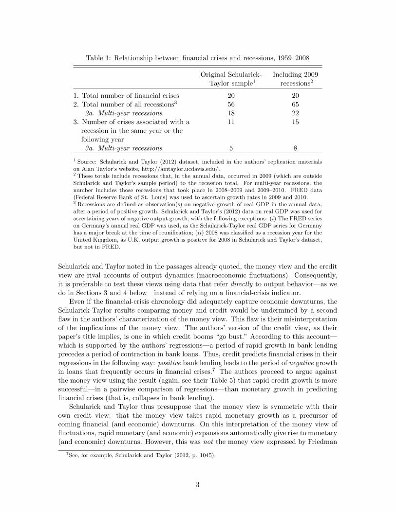
Table 1: Relationship between financial crises and recessions, 1959–2008

Original Schularick- Including 2009Taylor sample1 recessions2

1. Total number of financial crises 20 202. Total number of all recessions3 56 65

2a. Multi-year recessions 18 223. Number of crises associated with a 11 15

recession in the same year or thefollowing year

3a. Multi-year recessions 5 8

1 Source: Schularick and Taylor (2012) dataset, included in the authors’ replication materialson Alan Taylor’s website, http://amtaylor.ucdavis.edu/.2 These totals include recessions that, in the annual data, occurred in 2009 (which are outsideSchularick and Taylor’s sample period) to the recession total. For multi-year recessions, thenumber includes those recessions that took place in 2008–2009 and 2009–2010. FRED data(Federal Reserve Bank of St. Louis) was used to ascertain growth rates in 2009 and 2010.3 Recessions are defined as observation(s) on negative growth of real GDP in the annual data,after a period of positive growth. Schularick and Taylor’s (2012) data on real GDP was used forascertaining years of negative output growth, with the following exceptions: (i) The FRED serieson Germany’s annual real GDP was used, as the Schularick-Taylor real GDP series for Germanyhas a major break at the time of reunification; (ii) 2008 was classified as a recession year for theUnited Kingdom, as U.K. output growth is positive for 2008 in Schularick and Taylor’s dataset,but not in FRED.

Schularick and Taylor noted in the passages already quoted, the money view and the creditview are rival accounts of output dynamics (macroeconomic fluctuations). Consequently,it is preferable to test these views using data that refer directly to output behavior—as wedo in Sections 3 and 4 below—instead of relying on a financial-crisis indicator.

Even if the financial-crisis chronology did adequately capture economic downturns, theSchularick-Taylor results comparing money and credit would be undermined by a secondflaw in the authors’ characterization of the money view. This flaw is their misinterpretationof the implications of the money view. The authors’ version of the credit view, as theirpaper’s title implies, is one in which credit booms “go bust.” According to this account—which is supported by the authors’ regressions—a period of rapid growth in bank lendingprecedes a period of contraction in bank loans. Thus, credit predicts financial crises in theirregressions in the following way: positive bank lending leads to the period of negative growthin loans that frequently occurs in financial crises.7 The authors proceed to argue againstthe money view using the result (again, see their Table 5) that rapid credit growth is moresuccessful—in a pairwise comparison of regressions—than monetary growth in predictingfinancial crises (that is, collapses in bank lending).

Schularick and Taylor thus presuppose that the money view is symmetric with theirown credit view: that the money view takes rapid monetary growth as a precursor ofcoming financial (and economic) downturns. On this interpretation of the money view offluctuations, rapid monetary (and economic) expansions automatically give rise to monetary(and economic) downturns. However, this was not the money view expressed by Friedman

7See, for example, Schularick and Taylor (2012, p. 1045).

3

and Schwartz.8 On the contrary, Friedman and Schwartz (1963, p. 699) made their positionexplicit that the U.S. monetary collapse of the 1930s was “not an inevitable consequenceof what had gone before,” and Friedman (1964) indicated that, in his vision of cyclicalfluctuations, the scale of economic downturns was unrelated to the size of the precedingeconomic expansion. The Friedman-Schwartz money view of the cycle did not reflect abelief that output contractions flowed from monetary expansions; instead, they contendedthat, at the business cycle frequency, money tended to be positively correlated with currentand future output.

Consequently, from the perspective of the money view, if a period of negative monetaryand output growth occurs after a period of rapid monetary growth, this is likely a reflec-tion of the monetary policy decisions of the authorities—not of the structural relationshipbetween monetary fluctuations and economic fluctuations. Seen in this light, the results ofSchularick and Taylor (2012) indicating that rapid money growth is less useful than rapidlending growth in predicting financial crises do not provide evidence against the moneyview. That being so, it is desirable to examine more directly the money view’s predictionof a positive money/output relationship, as we do in this comment.

A third fault of Schularick and Taylor’s characterization of the money view is that,according to their account, advocates of money believe that monetary aggregates’ impor-tance arises from their ability to proxy the dynamics of credit. They take Friedman andSchwartz’s analysis of pre-World War II developments as having made the approximationthat money was a good stand-in for credit. Correspondingly, Schularick and Taylor take theincreased importance in the postwar period of wholesale deposits, and of other commercialbank liabilities that are often not counted in M2-type monetary aggregates, as ipso factoinvalidating the money view.9 However, advocates of the money view in the research litera-ture have not, in fact, rested their case on the notion that money and credit move together.On the contrary, the money view is recognized as depending on distinct transmission mech-anisms, such as portfolio balance channels, from those associated with the credit view (see,for example, Bordo and Schwartz, 1979, p. 56; Romer and Romer, 1990).10 Indeed, Fried-man (1970, pp. 18–22) was emphatic that his belief in money’s importance for economicfluctuations did not rest on any requirement that money and credit move together.11

The fourth reason why Schularick and Taylor (2012) do not adequately characterizethe money view is that, for many countries, their data on money are simply incorrect.Their undertaking of generating a “newly assembled dataset on money and credit” (p.1031) is to be applauded; and we condition on their credit data throughout our analysisbelow.12 But their monetary data contain major errors of two kinds: (1) For a few countries,their money series contains major untreated series breaks; a couple of key examples are

8Friedman and Schwartz (1963) and other Friedman monetary writings must serve as a key criterion forassessing what is meant by the money view. Schularick and Taylor (2012) refer to Friedman repeatedly and,as already indicated, specifically attribute the money view to him and Schwartz.

9See the quotation given above from Schularick and Taylor (2012, p. 1051), as well as their statement (p.1031) that “the ‘money view’ of the world looks entirely plausible” only under conditions in which moneyand credit move together.

10Bernanke (1983, 2012), although advocating the credit channel, acknowledged that the money channelis conceptually distinct and empirically important.

11That they do not in fact move together was a major message of Schularick and Taylor (2012) and onewe affirm below using our improved money series. However, as the Friedman (1970) discussion attests,Schularick and Taylor’s (2012) contention that advocates of money believed that money and credit movetogether is inaccurate.

12We also condition on Schularick and Taylor’s real GDP data (except in the case of Germany) andprice-level (CPI) data. We also follow their practice of ending the sample period in 2008.

4

highlighted below. Failure to allow for these breaks leads to materially lower money/outputcorrelations for these countries. (2) For the vast bulk of the countries in their sample, theannual observation on money is an end-of-period value, while standard theoretical andempirical approaches instead imply that the appropriate money variable is an average-of-period series.13 Schularick and Taylor’s (2012) use of end-of-period money produceschoppiness and unnecessary volatility in the annual observations on monetary growth—features that tend to make the correlation between money and output lower than it wouldotherwise be.

We improve on Schularick and Taylor’s money series by constructing, for the postwarperiod, “streamlined” broad money series for each of the countries in their study. LikeSchularick and Taylor’s money series, our streamlined monetary data are obtained fromnational and international data sources. But unlike Schularick and Taylor’s typical moneyseries, the streamlined monetary aggregates that we construct are adjusted for major seriesbreaks and consist of annual averages derived from the underlying monthly or quarterlymonetary data for each country.

We proceed in the next section to illustrate the importance of our use of streamlinedmoney series for the analysis of the postwar behavior of money and the dynamic correlationsof money and output. Then, in Section 4, we evaluate the money view and credit view interms of their ability to predict output contractions (recessions) in the postwar period(which, following Schularick and Taylor, we take as spanning through 2008). We find that,on this criterion, money has a more important and reliable relationship with macroeconomicoutcomes than does credit.

3 Comparisons of money series

For the fourteen countries considered by Schularick and Taylor (2012), we have constructedour own broad money series by obtaining annual averages from monthly or quarterly data.We commence these series in 1957 because that is when one key data source—the Interna-tional Monetary Fund’s International Financial Statistics (IFS )—starts reporting money-stock data for many countries on a monthly basis.14 In order to have a complete and (asfar as possible) break-free series for each country, we have used the IFS data in conjunctionwith information from other international databases as well as country-specific sources.Details of the construction of our monetary series are given in Appendix B.

We now illustrate, by considering a selection of countries’ data, a few of the advantagesof our streamlined monetary data over those compiled by Schularick and Taylor (2012).

13Even if, contrary to standard practice, end-of-period money was deemed the series of interest, Schularickand Taylor’s use of money in their regressions would be invalid. Money in these regressions is a real moneyseries obtained by deflating money by the price level. Schularick and Taylor’s (2012) price-level series foreach country is an annual-average series. Therefore, their observations on real money typically consist of anend-of-period series divided by an average-of-period series—an invalid combination.

14Defining the postwar period as starting in the late 1950s also has the virtue of omitting the immediatepost-World War II years, in which wartime economic controls remained prevalent in several countries, aswell as the Korean War period.

5

Figure 1: Measures of nominal broad money growth

3.1 Selected country comparisons

As already indicated, our monetary series are average-of-year variables. The Schularick andTaylor (2012) series, in contrast, are primarily end-of-year data.15 The difference impliedby our more valid approach to time aggregation of money is demonstrated in Figure 1,which compares the monetary-growth data arising from the two approaches. The firstpanel of Figure 1 shows U.S. broad money growth series from the two datasets. In bothcases, money is measured by M2, but Schularick and Taylor’s M2 growth series exhibitsgreater choppiness; this exemplifies the extra variability in series that typically arises fromthe sampling of end-of-year values instead of annual averages. It is also important to notean additional problem: the use of end-of-year data for period t leads to a money seriesthat refers to a date later than their observation for period-t output (which is an annualaverage). Consequently, for any year’s observations, Schularick and Taylor’s monetary datain effect refer to a period following the period associated with the output data. This impliesthat evaluations of the dynamic relationship between the growth rates of money and outputwould not be reliable if one used the Schularick-Taylor monetary series.

The volatility of end-of-year data on money is also evident in the next country consid-ered: the Netherlands. As the top-right panel of Figure 1 shows, our streamlined series formonetary growth in this country is smoother than the Schularick-Taylor series. A further

15In the case of Norway, Schularick and Taylor (2012) evidently use average-of-year data on money forsubstantial parts of the postwar period. That is, while Schularick and Taylor (2012) predominantly useend-of-year data on money, they do not follow this practice consistently across countries.

6

problem in this instance is that Schularick and Taylor’s money series for Netherlands hasa very severe break (of well over 50 percent of the level of the series) in the early 1980s.This break—clearly visible in the panel—has a material effect on the correlation betweenreal broad money growth and the same year’s output growth for the Netherlands. UsingSchularick and Taylor’s data on money, this correlation is negative and insignificant for1959–2008 (−0.13). In contrast, when our streamlined series for the Netherlands’ monetarygrowth (a series that relies on sources that avoid the break) is used for the same period,there is a positive and statistically significant correlation (0.32).

The third country we consider is France (bottom-left panel of Figure 1). Schularickand Taylor’s monetary growth series for France displays a sharp series break in 1970; inour construction of a streamlined money series from data sources for France, we avoid thisbreak. Our streamlined series for France’s money stock has a notably stronger relationshipwith France’s real GDP than does Schularick and Taylor’s series. For example, for 1959–2008, the correlation between real money growth and the same year’s output growth is 0.21using Schularick and Taylor’s money series, compared with 0.53 using our money series.

The final country we consider in these selected comparisons is the United Kingdom(bottom-right panel of Figure 1). In describing their data, Schularick and Taylor (2009,p. 32) give the money series they use as “M2 or M3.” In fact, for the final few decadesof their sample period, Schularick and Taylor used neither M2 nor M3 in measuring U.K.broad money. The M3 series for the United Kingdom was abolished in 1989, so it was notavailable as a monetary measure in recent decades; furthermore, Schularick and Taylor didnot measure U.K. money by M2. Rather, they actually used (end-of-period) M4. However,an M2 series (also called “Retail M4”) is available in the Bank of England’s databasestarting in mid-1982; and we use this series’ annual average to compute monetary growthfrom 1984 onward. Over 1984 to 2008, the resulting M2 growth series and Schularick andTaylor’s series on U.K. monetary growth often behaved very differently, as is brought outin Figure 1.

In order to have a money series that covers the years prior to the early 1980s—theperiod for which U.K. M2 data are not available—we have constructed two alternativeU.K. monetary series: one (“streamlined”) using annual averages of M1 data and the other(“alternative streamlined”) using annual averages of a broader U.K. monetary total. Bothseries are joined to the U.K. M2 series that begins in the 1980s; consequently, although weuse two streamlined money series for the United Kingdom, the two series have identicalgrowth rates from 1984 onward, as Figure 1 indicates. In our empirical exercises below, weprovide results using each version of our streamlined U.K. monetary series.

3.2 Overall comparisons of the money series

Table 2 provides evidence on the differences between the Schularick-Taylor and streamlinedmonetary-growth series by reporting series means and standard deviations. The moneyseries tend to have similar means in each country, but the Schularick-Taylor series almostinvariably have larger standard deviations. This difference reflects the extra measurementerror induced by approximating money’s behavior for the whole year by its value in a singlemonth.

As already noted, Schularick and Taylor (2012) judged the money/output and money/credit relationships only indirectly, on the basis of the relationship between the aggregatesand financial crises. However, direct examination of the relationship between financialaggregates and output is preferable. We pursue this matter in Section 4. As preliminary

7

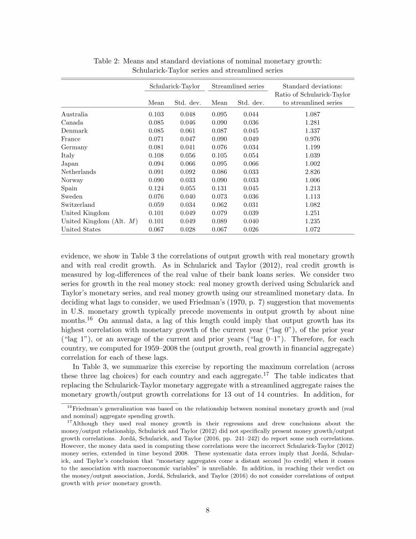
Table 2: Means and standard deviations of nominal monetary growth:Schularick-Taylor series and streamlined series

Schularick-Taylor Streamlined series Standard deviations:Ratio of Schularick-Taylor

Mean Std. dev. Mean Std. dev. to streamlined series

Australia 0.103 0.048 0.095 0.044 1.087Canada 0.085 0.046 0.090 0.036 1.281Denmark 0.085 0.061 0.087 0.045 1.337France 0.071 0.047 0.090 0.049 0.976Germany 0.081 0.041 0.076 0.034 1.199Italy 0.108 0.056 0.105 0.054 1.039Japan 0.094 0.066 0.095 0.066 1.002Netherlands 0.091 0.092 0.086 0.033 2.826Norway 0.090 0.033 0.090 0.033 1.006Spain 0.124 0.055 0.131 0.045 1.213Sweden 0.076 0.040 0.073 0.036 1.113Switzerland 0.059 0.034 0.062 0.031 1.082United Kingdom 0.101 0.049 0.079 0.039 1.251United Kingdom (Alt. M ) 0.101 0.049 0.089 0.040 1.235United States 0.067 0.028 0.067 0.026 1.072

evidence, we show in Table 3 the correlations of output growth with real monetary growthand with real credit growth. As in Schularick and Taylor (2012), real credit growth ismeasured by log-differences of the real value of their bank loans series. We consider twoseries for growth in the real money stock: real money growth derived using Schularick andTaylor’s monetary series, and real money growth using our streamlined monetary data. Indeciding what lags to consider, we used Friedman’s (1970, p. 7) suggestion that movementsin U.S. monetary growth typically precede movements in output growth by about ninemonths.16 On annual data, a lag of this length could imply that output growth has itshighest correlation with monetary growth of the current year (“lag 0”), of the prior year(“lag 1”), or an average of the current and prior years (“lag 0–1”). Therefore, for eachcountry, we computed for 1959–2008 the (output growth, real growth in financial aggregate)correlation for each of these lags.

In Table 3, we summarize this exercise by reporting the maximum correlation (acrossthese three lag choices) for each country and each aggregate.17 The table indicates thatreplacing the Schularick-Taylor monetary aggregate with a streamlined aggregate raises themonetary growth/output growth correlations for 13 out of 14 countries. In addition, for

16Friedman’s generalization was based on the relationship between nominal monetary growth and (realand nominal) aggregate spending growth.

17Although they used real money growth in their regressions and drew conclusions about themoney/output relationship, Schularick and Taylor (2012) did not specifically present money growth/outputgrowth correlations. Jorda, Schularick, and Taylor (2016, pp. 241–242) do report some such correlations.However, the money data used in computing these correlations were the incorrect Schularick-Taylor (2012)money series, extended in time beyond 2008. These systematic data errors imply that Jorda, Schular-ick, and Taylor’s conclusion that “monetary aggregates come a distant second [to credit] when it comesto the association with macroeconomic variables” is unreliable. In addition, in reaching their verdict onthe money/output association, Jorda, Schularick, and Taylor (2016) do not consider correlations of outputgrowth with prior monetary growth.

8

Table 3: Dynamic correlations of output growth with monetary and credit series,1959–2008

Real loans growth Real broad money Real broad moneygrowth (Schularick- growth (streamlinedTaylor series) series)

Australia 0.393 (lag 0) 0.546 (lag 0) 0.551 (lag 0)Canada 0.457 (lag 0) 0.389 (lag 0–1) 0.482 (lag 0–1)Denmark 0.285 (lag 0) 0.294 (lag 0–1) 0.477 (lag 0–1)France 0.541 (lag 0–1) 0.309 (lag 1) 0.580 (lag 0–1)Germany 0.549 (lag 1) 0.524 (lag 1) 0.641 (lag 1)Germany (Alt. GDP) 0.708 (lag 0–1) 0.651 (lag 0–1) 0.766 (lag 0–1)Italy 0.500 (lag 0–1) 0.570 (lag 1) 0.617 (lag 1)Japan 0.688 (lag 0–1) 0.797 (lag 0–1) 0.808 (lag 0–1)Netherlands 0.437 (lag 0–1) 0.024 (lag 1) 0.327 (lag 0–1)Norway 0.180 (lag 0) 0.176 (lag 0) 0.194 (lag 0)Spain 0.337 (lag 0–1) 0.623 (lag 0–1) 0.699 (lag 0–1)Sweden 0.153 (lag 0–1) 0.374 (lag 0–1) 0.415 (lag 1)Switzerland 0.583 (lag 1) 0.616 (lag 1) 0.660 (lag 1)United Kingdom 0.609 (lag 0) 0.468 (lag 0) 0.545 (lag 0–1)United Kingdom (Alt. M ) 0.609 (lag 0) 0.468 (lag 0) 0.440 (lag 0)United States 0.656 (lag 0) 0.587 (lag 1) 0.537 (lag 1)

Note: As the correlations are obtained from a sample of 50 observations, correlations arestatistically significant at the conventional 5 per cent level if they exceed about 0.275 inabsolute value. “Alt. GDP” uses FRED data on Germany’s real GDP.

11 out of 14 countries, the correlation between streamlined monetary growth and outputgrowth is higher than the correlation between credit growth and output growth. And inthe case of those countries (the United Kingdom, the Netherlands, and the United States)for which the credit/output correlation is higher than the money/output correlation, thelatter correlation is uniformly significantly positive and, in certain cases, fairly sizable.Specifically, the value of the correlation is 0.33 for the Netherlands, 0.55 for the UnitedKingdom (or 0.44 using the alternative U.K. money series), and 0.54 for the United States.

4 Money versus credit as recession predictors

As indicated earlier, Schularick and Taylor (2012) compared the ability of credit growthand monetary growth to account for macroeconomic outcomes by performing separate logitregressions, thereby ascertaining the effect of each of these financial variables on the prob-ability of the onset of a financial crisis. However, as documented in Section 2 above, not allfinancial crises are associated with recessions, and many recessions are not associated withfinancial crises. A more appropriate approach in evaluating the usefulness of the moneyview and the credit view—which are both accounts of macroeconomic fluctuations—woulduse information on recessions directly. That approach is the focus of this section.

As a preliminary step, we re-run Schularick and Taylor’s (2012, Table 5) main regression

9

for their 14-country dataset for our sample period of 1963–2008.18 The regression sampleperiod starts in 1963 because our data on streamlined monetary growth start in 1958 andregressors such as monetary growth appear with five lags in Schularick and Taylor’s (2012)regressions.19 The regression specification is as follows:

logit(pit) = b0i + b1(L)DlogCREDITit + eit (1)

where logit(pit) = log( pit1−pit ) is the log of the odds ratio of a financial crisis for country i

in year t and b0i is a country-specific intercept term. As already indicated, specification(1) includes lags 1–5 of each variable. The variable CREDITit stands for the Schularick-Taylor real credit (specifically, bank loans) series; it will be replaced by real money in someregressions. Just as in Table 3 above, this real credit series is defined as total bank loansdeflated by the CPI, and it enters the regression in log first-differenced form. In columns(1.2) to (1.4) of Table 4, lags of real credit growth are replaced by lags of real monetarygrowth (Schularick and Taylor’s series, then the two sets of our streamlined money series).The lag polynomial b1(L) summarizes the relationship between the probability of a financialcrisis and the lagged values of the real growth in the financial aggregate (credit or money).A positive b1 coefficient would suggest that high credit (or monetary) growth in a precedingperiod portends a financial crisis. The error term is denoted by eit.

In Table 4, we report the results of the above regression specification for our sampleperiod; we include the regression summary statistics reported by Schularick and Taylor(2012). Our results do not overturn Schularick and Taylor’s finding that credit is a betterpredictor of financial crises than money. The individual and summed coefficients on creditgrowth tend to be more negative and more statistically significant than those on monetarygrowth (whether using Schularick and Taylor’s money series or our streamlined series), whilethe regression with credit growth has a better fit, as measured by the pseudo-R2. However,as indicated above, we do not see the money view as predicting that rapid monetary growthforeshadows financial crises, so we do not regard regression results of this kind as evidenceagainst the money view. Furthermore, we argued above that financial-crisis prediction doesnot provide a valid basis for assessing the ability of the money view and the credit view toaccount for macroeconomic fluctuations.

We perform a more valid assessment in the next regression specification by examining therelationship of these variables with output directly. This will also bring out the importanceof our use of the streamlined monetary series.

The results of this more valid test are reported in Table 5. The table reports logitregressions for the probability of the onset of a recession (that is, of the first year of negativegrowth) for 1963–2008 in Schularick and Taylor’s 14-country dataset. The specificationfollows that of Schularick and Taylor (2012), given in equation (1) above, except that the

18We have used the replication code provided by the authors among the replication materials for their pa-per at Alan Taylor’s website http://amtaylor.ucdavis.edu/; the later regressions are obtained from this codeusing our new dependent variables. As already indicated, although this dataset covers fourteen countries,the financial-crisis regressions in Schularick and Taylor’s (2012) Table 5 does not include Canada, whichdid not have a financial crisis in their postwar chronology. Correspondingly, our regressions in Table 4 alsoexclude Canada. As all countries had recessions in the 1963–2008 period, all countries are included in ourlater regressions (such as those in Tables 5 and 6 below).

19Schularick and Taylor’s (2012) postwar regressions use a sample period of 1953–2008; due to the fiveannual lags in the regressions, the regressions use data on the right-hand-side variables back to 1948. Wesuccessfully replicated the postwar regressions in their Tables 4 and 5 (pp. 1048–1049), before estimatingour own regressions for the 1963–2008 period.

10

Table 4: Logit regressions for prediction of financial crisis

Dependent variable: Log odds ratio for start of financial crisis

(1.1) (1.2) (1.3) (1.4)

1963–2008 1963–2008 1963–2008 1963–2008 usingusing loans replacing loans with using streamlined broad

broad money streamlined money, alternativeVARIABLES broad money U.K. series used

L. ∆ (loans/P) −0.478 3.283 4.850 5.997(3.374) (4.168) (8.186) (8.858)

L2. ∆ (loans/P) 9.582∗∗∗ 4.834∗∗ −2.919 −2.146(2.940) (2.362) (6.126) (5.815)

L3. ∆ (loans/P) 3.601 4.274∗∗ 9.030 6.424(2.914) (2.178) (5.997) (6.354)

L4. ∆ (loans/P) 0.482 −0.870 −8.217 −3.137(3.003) (5.698) (8.066) (7.624)

L5. ∆ (loans/P) −1.505 0.816 6.622 5.474(3.694) (4.085) (7.005) (7.589)

Observations 598 598 598 598Marginal effects at −0.0108 0.0878 0.133 0.165each lag evaluated 0.217 0.129 −0.0799 −0.0590at the means 0.0817 0.114 0.247 0.177

0.0109 −0.0233 −0.225 −0.0863−0.0342 0.0218 0.181 0.151

Sum 0.265 0.330 0.256 0.347Sum of lag coefficients 11.680∗∗ 12.340∗∗ 9.365 12.610∗

Standard error 5.890 6.151 7.139 7.459Test for all lags, = 0, χ2 11.860∗∗ 12.150∗∗ 5.454 4.395p-value 0.0367 0.0327 0.363 0.494Test for country effects, = 0, χ2 6.291 5.950 7.287 6.821p-value 0.901 0.919 0.838 0.869Pseudo R2 0.0909 0.0520 0.0460 0.0441Pseudolikelihood −79.650 −83.070 −83.590 −83.750Overall test statistic, χ2 33.300∗∗ 19.580 11.200 13.490p-value 0.0103 0.296 0.846 0.703AUROC 0.727∗∗∗ 0.671∗∗∗ 0.664∗∗∗ 0.679∗∗∗

Standard error 0.0671 0.0602 0.0604 0.0574

*** p < 0.01, ** p < 0.05, * p < 0.10

Note: Fixed effects are estimated throughout. Robust standard errors are given in parentheses.

dependent variable is redefined:

logit(prit) = b0i + b1(L)DlogCREDITit + eit (2)

where logit(prit) = log(prit

1−prit) now corresponds to the log of the odds ratio for a recession

for country i starting in year t. As before, we consider in succession their real creditgrowth using their loans series, real monetary growth using their broad money series, andreal monetary growth using our streamlined broad money series. We continue to follow

11

Schularick and Taylor’s lag length of five years (that is, lags 1 to 5 of the financial series).20

Three features are notable in the results in Table 5. First, irrespective of money seriesused, the terms in monetary growth are jointly statistically significant. The lag polynomialfor monetary growth also has a negative coefficient sum. This implies a positive relationshipbetween money and output over the business cycle, as suggested by the money view ofFriedman and Schwartz (1963). Schularick and Taylor (2012) found that rapid credit growthpredicts financial crises and does so better than monetary growth—results that we havefound in Table 4 continue to hold on the 1963–2008 sample period and with our streamlinedmoney series. But this regularity does not imply that the money view provides a pooraccount of macroeconomic outcomes, as the money view does not predict a structuralrelationship between easy money and subsequent economic or financial downturns (i.e., itdoes not predict a positive regression coefficient). However, the money view does implythat recessions tend to be preceded by weakness in monetary growth (so that there is anegative regression coefficient on money)—and our results confirm this prediction.21

Second, monetary growth outperforms credit growth in the regressions, irrespective ofmoney series used. Money enters with a more sizable coefficient sum than credit (i.e., morenegative coefficient sums than credit) and the regressions with money also have a better fitthan those with credit, by the criterion of the pseudo-R2. These results support the notionthat the money view’s success in accounting for macroeconomic fluctuations does not restfundamentally on money being a proxy for loans or bank credit.22

Third, monetary growth’s significance in the regressions increases when we use ourstreamlined monetary series, consistent with these series providing better measurement ofmoney than Schularick and Taylor’s (2012) data.

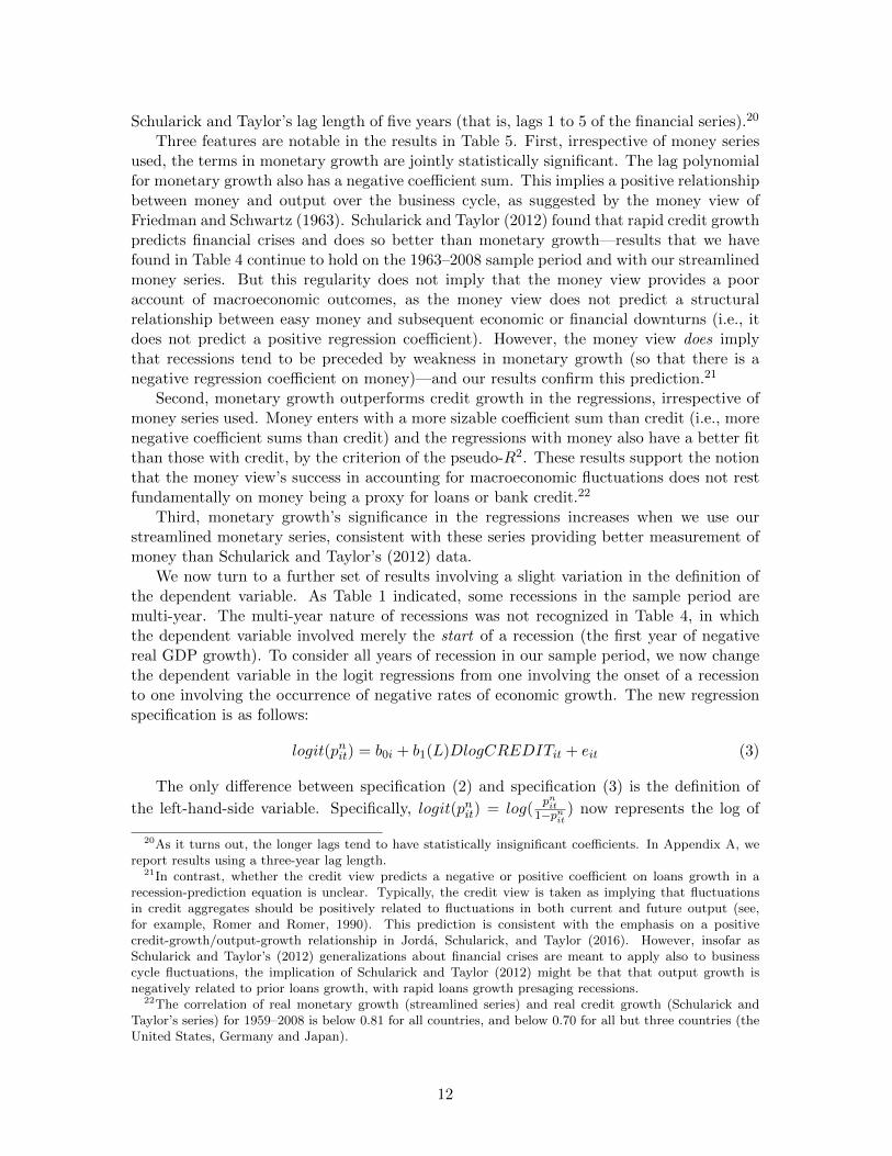
We now turn to a further set of results involving a slight variation in the definition ofthe dependent variable. As Table 1 indicated, some recessions in the sample period aremulti-year. The multi-year nature of recessions was not recognized in Table 4, in whichthe dependent variable involved merely the start of a recession (the first year of negativereal GDP growth). To consider all years of recession in our sample period, we now changethe dependent variable in the logit regressions from one involving the onset of a recessionto one involving the occurrence of negative rates of economic growth. The new regressionspecification is as follows:

logit(pnit) = b0i + b1(L)DlogCREDITit + eit (3)

The only difference between specification (2) and specification (3) is the definition of

the left-hand-side variable. Specifically, logit(pnit) = log(pnit

1−pnit) now represents the log of

20As it turns out, the longer lags tend to have statistically insignificant coefficients. In Appendix A, wereport results using a three-year lag length.

21In contrast, whether the credit view predicts a negative or positive coefficient on loans growth in arecession-prediction equation is unclear. Typically, the credit view is taken as implying that fluctuationsin credit aggregates should be positively related to fluctuations in both current and future output (see,for example, Romer and Romer, 1990). This prediction is consistent with the emphasis on a positivecredit-growth/output-growth relationship in Jorda, Schularick, and Taylor (2016). However, insofar asSchularick and Taylor’s (2012) generalizations about financial crises are meant to apply also to businesscycle fluctuations, the implication of Schularick and Taylor (2012) might be that that output growth isnegatively related to prior loans growth, with rapid loans growth presaging recessions.

22The correlation of real monetary growth (streamlined series) and real credit growth (Schularick andTaylor’s series) for 1959–2008 is below 0.81 for all countries, and below 0.70 for all but three countries (theUnited States, Germany and Japan).

12

Table 5: Logit regressions for prediction of onset of recessions, all countries

Dependent variable: Log odds ratio for recession start

(2.1) (2.2) (2.3) (2.4)



L. ∆ (loans/P) −5.120∗ −9.369∗∗ −18.280∗∗∗ −17.130∗∗∗

(2.975) (3.697) (4.605) (4.521)L2. ∆ (loans/P) 2.985 3.090 7.473 5.690

(2.480) (2.420) (5.161) (5.020)L3. ∆ (loans/P) 4.117∗ 2.479 1.377 2.130

(2.406) (2.420) (5.228) (5.488)L4. ∆ (loans/P) 1.380 −2.033 3.270 2.664

(2.417) (2.917) (5.257) (5.394)L5. ∆ (loans/P) −2.162 2.382 1.289 0.578

(2.183) (2.768) (4.123) (4.346)

Observations 644 644 644 644Marginal effects at −0.342 −0.623 −1.147 −1.096each lag evaluated 0.199 0.206 0.469 0.364at the means 0.275 0.165 0.0864 0.136

0.0921 −0.135 0.205 0.170−0.144 0.158 0.0808 0.0370

Sum 0.0801 −0.230 −0.306 −0.388Sum of lag coefficients 1.200 −3.452 −4.873 −6.066Standard error 3.829 5.041 6.090 6.298Test for all lags, = 0, χ2 8.880 9.457∗ 17.440∗∗∗ 15.100∗∗∗

p-value 0.114 0.0922 0.00374 0.00993Test for country effects, = 0, χ2 8.003 6.919 5.501 5.357p-value 0.843 0.906 0.962 0.966Pseudo R2 0.0450 0.0458 0.0754 0.0672Pseudolikelihood −174.900 −174.700 −169.300 −170.800Overall test statistic, χ2 17.010 17.490 28.790∗ 26.750∗

p-value 0.522 0.490 0.0510 0.0837AUROC 0.680∗∗∗ 0.665∗∗∗ 0.738∗∗∗ 0.721∗∗∗

Standard error 0.0374 0.0409 0.0340 0.0347

*** p < 0.01, ** p < 0.05, * p < 0.10

Note: Equation estimated is specification (2) in text. Dates of recession starts during 1963–2008 areascertained as described in Table 1. Fixed effects are estimated throughout. Robust standard errorsare given in parentheses.

the odds ratio of a period of negative growth for country i in year t.23 The results continueto favor money over credit and our streamlined money series over the Schularick-Taylormoney series. Again, in the columns labeled (3.2) to (3.4) of Table 6, real credit growth isreplaced with real monetary growth.

23That is, the dependent variable is constructed using an indicator variable that is equal to 1 in each yearof negative growth, and 0 otherwise, instead of taking nonzero values only for the first year of a recession.

13

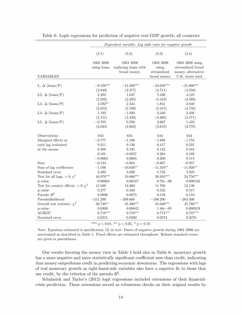
Table 6: Logit regressions for prediction of negative real GDP growth, all countries

Dependent variable: Log odds ratio for negative growth

(3.1) (3.2) (3.3) (3.4)



L. ∆ (loans/P) −9.198∗∗∗ −14.380∗∗∗ −24.650∗∗∗ −21.860∗∗∗

(2.849) (3.477) (4.711) (4.558)L2. ∆ (loans/P) 2.492 1.637 5.436 4.125

(2.502) (2.285) (4.410) (4.389)L3. ∆ (loans/P) 4.592∗∗ 2.344 1.851 2.048

(2.053) (2.196) (4.415) (4.732)L4. ∆ (loans/P) 1.193 −1.030 3.440 2.348

(2.151) (2.420) (4.268) (4.471)L5. ∆ (loans/P) −0.785 0.798 2.607 1.423

(2.034) (2.603) (3.610) (3.776)


0.101 −0.0857 0.264 0.189−0.0663 0.0664 0.200 0.114

Sum −0.144 −0.884 −0.867 −0.957Sum of lag coefficients −1.706 −10.630∗∗ −11.310∗∗ −11.920∗∗

Standard error 3.493 5.030 5.758 5.925Test for all lags, = 0, χ2 16.070∗∗∗ 19.060∗∗∗ 30.910∗∗∗ 24.750∗∗∗

p-value 0.00664 0.00187 9.78e−06 0.000156Test for country effects, = 0, χ2 15.500 13.360 11.700 12.130p-value 0.277 0.420 0.552 0.517Pseudo R2 0.0806 0.0875 0.133 0.110Pseudolikelihood −211.200 −209.600 −199.200 −204.400Overall test statistic, χ2 30.740∗∗ 35.400∗∗∗ 54.640∗∗∗ 45.780∗∗∗

p-value 0.0309 0.00842 1.46e−05 0.000319AUROC 0.718∗∗∗ 0.719∗∗∗ 0.774∗∗∗ 0.757∗∗∗

Standard error 0.0315 0.0330 0.0274 0.0278

*** p < 0.01, ** p < 0.05, * p < 0.10

Note: Equation estimated is specification (3) in text. Dates of negative growth during 1963–2008 areascertained as described in Table 1. Fixed effects are estimated throughout. Robust standard errorsare given in parentheses.

Our results favoring the money view in Table 5 hold also in Table 6: monetary growthhas a more negative and more statistically significant coefficient sum than credit, indicatingthat money outperforms credit in predicting economic downturns. The regressions with lagsof real monetary growth as right-hand-side variables also have a superior fit to those thatuse credit, by the criterion of the pseudo-R2.

Schularick and Taylor’s (2012) logit regressions included extensions of their financial-crisis prediction. These extensions served as robustness checks on their original results by

14

Table 7: Robustness exercises


Baseline Baseline Baseline Baseline Baselineplus plus plus plus plus

5 lags of 5 lags of 5 lags of 5 lags of 5 lags ofFinancial real GDP inflation nominal real short- change invariable growth short-term term int. I/Y

int. rate rate

Loans Sum of lag coefficients 3.978 −3.082 3.542 4.602 −1.364Standard error 5.158 4.246 4.793 4.951 4.408Pseudo R2 0.069 0.113 0.175 0.098 0.063Observations 644 644 570 570 644

Schularick- Sum of lag coefficients −2.123 −9.415∗ 0.626 3.973 −7.693Taylor Standard error 6.948 5.617 6.817 6.013 5.694money series Pseudo R2 0.064 0.103 0.180 0.086 0.064

Observations 644 644 570 570 644

Streamlined Sum of lag coefficients −0.760 −9.847 −1.413 2.142 −9.402money Standard error 9.322 6.770 8.491 8.089 6.791series Pseudo R2 0.084 0.114 0.174 0.121 0.090

Observations 644 644 570 570 644

Streamlined Sum of lag coefficients −3.559 −12.690∗ −2.893 1.615 −11.210money Standard error 9.915 6.798 8.655 8.287 6.980series (using alt. Pseudo R2 0.078 0.114 0.170 0.117 0.085U.K. M series) Observations 644 644 570 570 644

*** p < 0.01, ** p < 0.05, * p < 0.10

Note: Data for additional regressors is from the Schularick-Taylor (2012) database, with the exception ofthe investment/output ratio for Germany for 1957–1959, and France for 1957–1958, for which theirobservations were missing. We obtained the observations for Germany from European Conference ofMinisters of Transport (1964, Annex Table 1), and for France from FRED, and they were arithmeticallyspliced into the Schularick-Taylor series on the investment/output ratio.

augmenting the financial-crisis prediction specification (1) with additional regressors: lags ofa number of additional macroeconomic variables, including real GDP growth, inflation, thenominal short-term interest rate and the corresponding real interest rate, and the change inthe investment/output ratio. We now carry out analogous extensions for our own estimatedspecifications. For the case in which the dependent variable pertains to the probability ofa recession start, the estimated equation becomes:

logit(prit) = b0i + b1(L)DlogCREDITit + b2(L)Xit + eit (4)

This specification differs from specification (2) in that the vector of variables Xit containsthe aforementioned macroeconomic variables.

In Table 7, we summarize the outcome of adding these additional regressors. In theregressions that include interest-rate variables, there is a substantial drop in the numberof observations in the regressions. Partly for this reason, both money and credit tend tolose significance when the additional regressors are included. Moreover, for the robustnesstests that include lagged real GDP growth, interpretation of the regressions is complicated

15

Table 8: Further robustness exercises


Baseline Baseline Baseline Baseline Baselineplus plus plus plus plus

5 lags of 5 lags of 5 lags of 5 lags of 5 lags ofFinancial real GDP inflation nominal real short- change invariable growth short-term term int. I/Y

int. rate rate

Loans Sum of lag coefficients 3.396 −5.518 0.422 1.258 −4.529Standard error 4.911 4.114 4.62 4.443 4.262Pseudo R2 0.178 0.142 0.215 0.132 0.110Observations 644 644 570 570 644

Schularick- Sum of lag coefficients −5.591 −17.450∗∗∗ −5.488 −3.228 −14.520∗∗

Taylor Standard error 6.709 5.565 6.265 5.851 5.852money series Pseudo R2 0.186 0.147 0.226 0.115 0.130

Observations 644 644 570 570 644

Streamlined Sum of lag coefficients −0.644 −15.690∗∗ −6.236 −4.541 −15.340∗∗

money Standard error 8.291 6.260 7.662 7.499 6.382series Pseudo R2 0.204 0.166 0.229 0.169 0.160

Observations 644 644 570 570 644

Streamlined Sum of lag coefficients −2.023 −18.170∗∗∗ −6.741 −3.742 −16.300∗∗

money Standard error 8.808 6.304 7.883 7.574 6.536series (using alt. Pseudo R2 0.190 0.153 0.217 0.150 0.140U.K. M series) Observations 644 644 570 570 644

*** p < 0.01, ** p < 0.05, * p < 0.10

Note: See notes to Tables 6 and 7.

by the fact that lagged real GDP growth enters into the construction of the left-hand-sidevariable. Notwithstanding these caveats, the robustness results, like the earlier results, tendto favor money over credit in predicting recessions. In particular, for all specifications, thesum of the lag coefficients on money (irrespective of money series) shows a tendency to bemore negative than does credit.

When inflation and the change in the investment-to-output ratio are the additionalregressors, real monetary growth continues to have a negative coefficient sum, and thissum remains larger in absolute value than that of real loans growth in the correspondingregressions using credit. When other additional right-hand-side variables are included—particularly the real interest rate—there is some tendency for the coefficients on real mon-etary growth and real credit growth to change sign, becoming positive. This tendency ismore pronounced in the case of real credit growth.

In Table 8, the same robustness results are reported for the case in which the dependentvariable refers (as in specification (3)) to the incidence of negative growth. Even more sothan in the recession-start regressions of Table 7, real monetary growth displays a tendencyto maintain a negative coefficient sum in the presence of the added regressors, and this sumis larger in absolute value than that on real loans growth. Notably, real monetary growthmaintains negative coefficient sums when the interest-rate variables are included, while thisis not true for real loans growth.

16

Overall, the robustness exercises reported in Tables 7 and 8 continue to favor moneyover credit in predicting macroeconomic fluctuations. In particular, these results suggestthat, for the postwar decades leading up to the 2008 financial crisis, judgments about theimportance of the link between lending aggregates and business cycles are more sensitiveto the inclusion of additional regressors than are judgments concerning the link betweenmonetary aggregates and business cycles. These robustness exercises therefore reinforce ourearlier results regarding the money view versus the credit view.

5 Conclusions

In this comment, we have reexamined Schularick and Taylor’s (2012) evaluation of themoney and credit views of macroeconomic fluctuations. For the postwar period, Schularickand Taylor conclude that the data strongly favor the credit view over the money view.However, Schularick and Taylor’s interpretation of the money view is faulty, as they see itsvalidity as requiring that rapid monetary growth predicts financial crises, and they take themoney view’s proponents as appealing to a proposition that changes in the money stockare a good proxy for changes in bank credit (specifically, bank loans). In fact, the moneyview of Friedman and Schwartz (1963) does not predict an automatic relationship betweenrapid monetary growth and (financial or economic) downturns, and it does not rest onmoney being a good proxy for credit. In addition, Schularick and Taylor’s (2012) data forbroad money have systematic errors resulting from their use of end-of-period instead ofaverage-of-period data, and their failure to take adequate account of discontinuities. Witha corrected series for monetary aggregates, we have found support for the money viewby direct examination of the relationship of money and output. For the final half-century(1959–2008) of the period covered by Schularick and Taylor’s multi-country dataset, we findthat our money series has a correlation with output that is competitive with, and usuallyslightly better than, that of Schularick and Taylor’s money and credit series. In addition, wefound that money outperforms credit in predicting economic downturns in the 14 countriesin Schularick and Taylor’s dataset. This result—which continued to hold in a variety ofrobustness exercises—suggests that the money view of macroeconomic fluctuations gives abetter description of five decades’ worth of international postwar historical data than doesthe credit view.

We note two caveats concerning our results. First, we have followed Schularick and Tay-lor (2012) in considering regressions that end in 2008, thereby largely excluding from oursample the major economic and financial disruptions that began in late 2008 and continuedin the following years. This approach is consistent with Schularick and Taylor’s (2012, p.1029) call for use of historical information, including confining the postwar period to theperiod through 2008, to examine the money and credit views. Recent years (that is, 2009onward) have presented new information, not used by us or by Schularick and Taylor (2012),relevant for discriminating between the money and credit views. This evidence could tipthe balance in favor of credit aggregates in understanding macroeconomic fluctuations. Ifit does so, however, one should consider this a break with pre-2009 postwar norms. Aswe have seen, the pre-2009 postwar record favors the money view over the credit view onthe criterion of predicting macroeconomic fluctuations. This result contrasts with Schu-larick and Taylor’s (2012, p. 1047) claim to have established a finding—which they notehas “broad implications for economic history”—that credit aggregates have been cruciallyimportant and monetary aggregates have not been.

17

Second, we have followed Schularick and Taylor (2012) by concentrating on monetaryand loan aggregates in representing the money and credit views. Evaluation of the relativemerits of the money and credit views, as well as the incorporation of both money and creditchannels into empirical models, would benefit from an examination of other kinds of data.For example, Divisia series might provide better measures of monetary aggregates, andBelongia and Ireland (2016) suggest that Divisia monetary series are more closely relatedto U.S. output fluctuations than are conventional measures of the U.S. money stock. Inaddition, it may be that both the money view and the credit view are better captured byasset-price reactions than by financial aggregates: for example, the credit channel likelyworks in part by affecting credit spreads, while the money channel involves a portfoliobalance mechanism that affects term premiums, among other variables.

18

References

Abildgren, Kim. 2009. “Monetary Regimes and the Endogeneity of Labour Market Struc-tures: Empirical Evidence from Denmark 1875–2007.” European Review of EconomicHistory, 13(2): 199–218.

Balke, Nathan, and Robert J. Gordon. 1986. “Appendix B: Historical Data.” InThe American Business Cycle: Continuity and Change. ed. by R.J. Gordon, Chicago:University of Chicago Press, 781–850.

Belongia, Michael T., and Peter N. Ireland. 2016. “Money and Output: Friedmanand Schwartz Revisited.” Journal of Money, Credit and Banking, 48(6): 1223–1266.

Bernanke, Ben S. 1983. “Nonmonetary Effects of the Financial Crisis in the Propagationof the Great Depression.” American Economic Review, 73(3): 257–276.

Bernanke, Ben S. 2012. “Opening Remarks: Monetary Policy Since the Onset of theCrisis.” In The Changing Policy Landscape: A Symposium Sponsored by the FederalReserve Bank of Kansas City. Kansas City, MO: Federal Reserve Bank of Kansas City,1–22. https://www.kansascityfed.org/publicat/sympos/2012/Bernanke final.pdf.

Bordo, Michael D., and Anna J. Schwartz. 1979. “Clark Warburton: Pioneer Mone-tarist.” Journal of Monetary Economics, 5(5): 43–65.

Bullock, Michele, Dirk Morris, and Glenn Stevens. 1988. “The Relationship BetweenFinancial Indicators and Economic Activity: 1968–1987.” Reserve Bank of AustraliaResearch Discussion Paper Series No. 8805.

Capie, Forrest H., and Alan Webber. 1985. A Monetary History of the United King-dom, 1870–1982, Volume 1: Data, Sources, Methods. London: George Allen and Unwin.

Den Butter, Frank A.G., and Martin M.G. Fase. 1981. “The Demand for Money inEEC Countries.” Journal of Monetary Economics, 8(2): 201–230.

Edvinsson, Rodney, and Anders Ogren. 2014. “Swedish Money Sup-ply, 1620–2012.” In Historical Monetary and Financial Statistics for Swe-den, Volume II: House Prices, Stock Returns, National Accounts, and theRiksbank Balance Sheet, 1620–2012. ed. by Rodney Edvinsson, Tor Ja-cobson, and Daniel Waldenstrom, Stockholm: Sveriges Riksbank, 293–338.http://www.riksbank.se/Documents/Forskning/%c3%96vrigt/2014/foa historical statistics %20volume2 140613.pdf.

European Conference of the Ministers of Transport. 1964. XIV Council of MinistersResolutions. Paris: OECD.

Friedman, Milton. 1964. “The Monetary Studies of the National Bureau.” In The Na-tional Bureau Enters Its 45th Year. New York: NBER, 7–25. Reprinted in The OptimumQuantity of Money and Other Essays, by Milton Friedman, ch. 12, pp. 261–84. Chicago:Aldine, 1969.

Friedman, Milton. 1970. “Controls on Interest Rates Paid by Banks.” Journal of Money,Credit and Banking, 2(1): 15–32.

19

Friedman, Milton, and Anna J. Schwartz. 1963. A Monetary History of the UnitedStates, 1867–1960. Princeton, N.J.: Princeton University Press.

Gertler, Mark, and Cara S. Lown. 1999. “The Information in the High-Yield BondSpread for the Business Cycle: Evidence and Some Implications.” Oxford Review ofEconomic Policy, 15(3): 132–150.

Gilchrist, Simon, and Egon Zakrajsek. 2012. “Credit Spreads and Business CycleFluctuations.” American Economic Review, 102(4): 1692–1720.

Hendry, David F., and Neil R. Ericsson. 1991. “Modeling the Demand for NarrowMoney in the United Kingdom and the United States.” European Economic Review,35(4): 833–881.

International Monetary Fund. 1983. International Financial Statistics Supplement onMoney. Washington, D.C.: International Monetary Fund.

Jorda, Oscar, Moritz Schularick, and Alan M Taylor. 2013. “When Credit BitesBack.” Journal of Money, Credit and Banking, 45(s2): 3–28.

Jorda, Oscar, Moritz Schularick, and Alan M. Taylor. 2016. “Macrofinancial Historyand the New Business Cycle Facts.” NBER Macroeconomics Annual, 31(1): 213–263.

Lothian, James R., Anthony Cassese, and Laura Nowak. 1983. “Data Appendix.”In The International Transmission of Inflation. ed. by Michael R. Darby and James R.Lothian, Chicago: University of Chicago Press, 525–718.

Martın-Acena, Pablo, and Marıa Angeles Pons Brıas. 2005. “Sistema monetario yfinanciero.” In Estadısticas historicas de Espana, siglos XIX–XX. ed. by A. Carreras andX. Tafunell, Madrid: Fundacion BBVA, 645–706.

Patat, Jean Pierre, and Michel Lutfalla. 1990. A Monetary History of France inthe Twentieth Century. Houndmills, U.K.: Macmillan, trans. by P. Martindale and D.Cobham.

Reinhart, Carmen M., and Kenneth S. Rogoff. 2009. This Time is Different: EightCenturies of Financial Folly. Princeton, N.J.: Princeton University Press.

Romer, Christina D., and David H. Romer. 1990. “New Evidence on the MonetaryTransmission Mechanism.” Brookings Papers on Economic Activity, 21(1): 149–198.

Romer, Christina D., and David H. Romer. 2017. “New Evidence on the Aftermathof Financial Crises in Advanced Countries.” American Economic Review, 107(10): 3072–3118.

Schularick, Moritz, and Alan M. Taylor. 2009. “Credit Booms Gone Bust: MonetaryPolicy, Leverage Cycles and Financial Crises, 1870–2008.” NBER Working Paper No.15512.

Schularick, Moritz, and Alan M. Taylor. 2012. “Credit Booms Gone Bust: MonetaryPolicy, Leverage Cycles, and Financial Crises, 1870–2008.” American Economic Review,102(2): 1029–1061.

20

Tortella, Gabriel, J. Garcıa Ruiz, and Jose Luis Garcıa Ruiz. 2013. Spanish Moneyand Banking: A History. London: Palgrave Macmillan.

White, R.C. 1973. Australian Banking and Monetary Statistics, 1945–1970. Sydney: Re-serve Bank of Australia.

21

A Additional results

Tab

leA

1:F

ull

resu

lts

for

corr

elat

ion

ofou

tpu

tgr

owth

wit

hre

alm

oney

grow

than

dre

alcr

edit

grow

th,

1959

–200

8

Cor

rela

tion

ofou

tpu

tC

orre

lati

onof

outp

ut

Cor

rela

tion

ofou

tpu

tgr

owth

and

real

mon

etar

ygr

owth

and

real

mon

etar

ygr

owth

and

real

cred

itgr

owth

(Sch

ula

rick

-Tay

lor

grow

th(s

trea

mli

ned

gro

wth

ofk

year

sea

rlie

rse

ries

)ofk

year

sea

rlie

rse

ries

)ofk

year

sea

rlie

r

k=

0k

=1

k=

0–1

k=

0k

=1

k=

0–1

k=

0k

=1

k=

0–1

Au

stra

lia

0.3

93−

0.0

790.1

900.

546

0.14

00.4

720.

551

0.16

90.4

35C

anad

a0.4

57−

0.0

820.2

500.

387

0.26

50.3

890.

399

0.39

70.4

82D

enm

ark

0.28

50.

055

0.1

870.

161

0.27

80.2

940.

470

0.33

70.4

77F

ran

ce0.

466

0.42

40.5

410.

205

0.30

90.3

020.

525

0.53

40.5

80G

erm

any

0.4

750.

549

0.5

450.

351

0.52

40.5

210.4

310.

641

0.6

17G

erm

any

(Alt

.G

DP

)0.

698

0.63

30.7

080.

497

0.59

80.6

510.6

310.

702

0.7

66It

aly

0.4

190.

443

0.5

000.

343

0.57

00.5

050.4

850.

617

0.5

95Jap

an

0.68

50.

556

0.6

880.

734

0.74

20.7

970.7

870.

699

0.8

08N

eth

erla

nd

s0.4

310.

290

0.4

37−

0.1

310.

024

−0.

081

0.3

180.

203

0.3

27N

orw

ay0.

180

0.02

30.1

260.

176

−0.

015

0.0

970.1

940.

011

0.1

27S

pain

0.2

710.

269

0.3

370.

556

0.55

70.6

230.6

410.

659

0.6

99S

wed

en0.

134

0.10

00.1

530.

236

0.35

40.3

740.2

360.

415

0.4

08S

wit

zerl

an

d0.

404

0.58

30.5

640.

277

0.61

60.5

140.3

760.

660

0.5

80U

nit

edK

ingd

om

0.6

090.

385

0.5

720.

468

0.24

60.4

060.5

160.

427

0.5

45U

nit

edK

ingd

om

(Alt

.M

)0.

609

0.38

50.5

720.

468

0.24

60.4

060.4

400.

199

0.3

64U

nit

edS

tate

s0.6

560.

201

0.4

940.

235

0.58

70.4

830.3

810.

537

0.5

26

Note

:A

sth

eco

rrel

ati

on

sare

obta

ined

from

asa

mp

leof

50ob

serv

atio

ns,

corr

elat

ion

sar

est

atis

tica

lly

sign

ifica

nt

atth

eco

nve

nti

on

al5

per

cent

leve

lif

they

exce

edab

out

0.27

5in

abso

lute

valu

e.

22

Table A2: Logit regression, prediction of onset of recessions, all countries:lag length for regressors restricted to three years


(2.5) (2.6) (2.7) (2.8)



L. ∆ (loans/P) −5.098∗ −9.413∗∗∗ −17.490∗∗∗ −16.750∗∗∗

(2.943) (3.631) (4.438) (4.447)L2. ∆ (loans/P) 3.015 3.302 6.668 5.081

(2.484) (2.381) (4.989) (4.905)L3. ∆ (loans/P) 4.307∗ 2.012 3.546 3.877

(2.251) (2.463) (4.471) (4.684)


0.00520 0.00446 0.00408 0.00406−0.0297 −0.0277 −0.0199 −0.0203

Sum 0.125 −0.298 −0.476 −0.516Sum of lag coefficients 2.225 −4.099 −7.272 −7.789Standard error 3.275 4.492 5.463 5.604Test for all lags, = 0, χ2 7.625∗ 7.787∗ 17.180∗∗∗ 15.040∗∗∗

p-value 0.0544 0.0506 0.000649 0.00178Test for country effects, = 0, χ2 8.238 6.909 5.537 5.354p-value 0.828 0.907 0.961 0.967Pseudo R2 0.0430 0.0437 0.0730 0.0660Pseudolikelihood −175.200 −175.100 −169.800 −171.000Overall test statistic, χ2 16.240 17.170 28.940∗∗ 26.600∗∗

p-value 0.436 0.375 0.0243 0.0461AUROC 0.680∗∗∗ 0.662∗∗∗ 0.735∗∗∗ 0.720∗∗∗

Standard error 0.0375 0.0404 0.0338 0.0346

*** p < 0.01, ** p < 0.05, * p < 0.10

Note: Equation estimated is specification (2) in text. See notes to Table 5.

23

Table A3: Logit regression, prediction of periods of negative growth, all countries:lag length for regressors restricted to three years


(3.5) (3.6) (3.7) (3.8)



L. ∆ (loans/P) −9.205∗∗∗ −14.450∗∗∗ −23.720∗∗∗ −21.530∗∗∗

(2.828) (3.453) (4.556) (4.501)L2. ∆ (loans/P) 2.494 1.736 4.364 3.511

(2.511) (2.258) (4.238) (4.326)L3. ∆ (loans/P) 4.985∗∗ 2.118 4.236 3.650

(1.947) (2.202) (4.044) (4.208)


0.00410 0.00300 0.00276 0.00287−0.0311 −0.0233 −0.00363 −0.00597

Sum −0.173 −0.903 −1.173 −1.159Sum of lag coefficients −1.726 −10.600∗∗ −15.120∗∗∗ −14.370∗∗∗

Standard error 2.994 4.313 5.196 5.245Test for all lags, = 0, χ2 16.180∗∗∗ 17.740∗∗∗ 30.420∗∗∗ 24.540∗∗∗

p-value 0.00104 0.000497 1.12e−06 1.93e−05Test for country effects, = 0, χ2 15.560 13.410 11.820 12.160p-value 0.274 0.417 0.543 0.515Pseudo R2 0.0800 0.0872 0.129 0.108Pseudolikelihood −211.300 −209.700 −200.100 −204.800Overall test statistic, χ2 30.780∗∗ 35.170∗∗∗ 54.390∗∗∗ 45.210∗∗∗

p-value 0.0144 0.00377 4.47e−06 0.000129AUROC 0.718∗∗∗ 0.718∗∗∗ 0.770∗∗∗ 0.756∗∗∗

Standard error 0.0312 0.0330 0.0275 0.0279

*** p < 0.01, ** p < 0.05, * p < 0.10

Note: Equation estimated is specification (3) in text. See notes to Table 6.

24

Figure A1: Measures of nominal broad money growth for remaining countries in the sample

25

B Details of the construction of streamlined broad moneyseries

This appendix describes the construction of the streamlined series on broad money thatwere used above as alternatives to the series constructed by Schularick and Taylor (2012).24

As indicated in the main text, a major criterion for our construction of broad monetaryaggregates (that is, M2 or a similar aggregate) has been that the series correspond, as faras possible, to average-of-year (that is, average of monthly observations) annual data—asopposed to the end-of-year monetary data predominantly used by Schularick and Taylor(2012). In those rare instances—indicated below—in which observations for the moneystock for every month of the year were not obtainable for a particular country, annual datahave been obtained as the average of the end-of-quarter observations on money (that is, asan average of four observations).

The annual sample period over which annual observations on monetary growth havebeen constructed here is the fifty-year period 1959–2008. This choice was in large partmotivated by the fact that monthly monetary data are not always clearly available formany countries for the period before 1957—the earliest year for which the electronic andhardcopy versions of the International Monetary Fund’s (IMF’s) International FinancialStatistics report monthly and/or quarterly observations on money.

As will be detailed below, the money-data construction has involved retrievals fromthe electronic version of the International Financial Statistics database (available on theIMF’s website) as well as consultation of national sources—electronic and hardcopy—onmonetary aggregates. In addition, two sources that tabulated time series for monetary datashould be mentioned as being of particular usefulness in the task of obtaining a completerun of cross-country monetary data for the whole 1959–2008 period. The first source isLothian, Cassese, and Nowak (1983). That study gave the results of an effort to construct,on a quarterly basis for the period from the 1950s to the mid-1970s, data on monetaryaggregates (among other series) for several advanced economies. The second key sourceis the International Monetary Fund’s (1983) International Financial Statistics Supplementon Money. This publication tabulated monthly IFS data on monetary aggregates for IMFmember countries for the period from 1967 to 1982. For some countries, the tabulationsin this IMF publication report monetary data that are not available in the modern-dayelectronic version of the IFS database.

Details of construction of broad money series for each country are provided below.

B.1 Australia

The broad money series for Australia used here corresponds to the series officially calledM3, spliced into the series officially called “Broad Money.”

The Reserve Bank of Australia (RBA) website provides monthly seasonally adjustedM3 data starting in July 1959. The annual averages of this series from 1960 onward wereused to calculate monetary growth (defined as log-differences) for Australia for 1961–1968.Pre-1961 observations on annual monetary growth were obtained from an annual averageof White’s (1973) total of currency and all bank deposits for the period 1956–1960. (The

24The authors are grateful to the following individuals for their help and advice on locating monetarydata for various countries: Kim Abildgren, Michael Bordo, Kimberly Doherty, Christina Gerberding, JesperLinde, Stefano Neri, Alasdair Scott, and Robert York.

26

log-differences of White’s series very closely match those of the official M3 series for 1961–1968.)

For the 1969–1977 period, monetary growth for Australia consists of the log-differencesof the annual averages of M3, with the annual averages obtained from the quarterly sea-sonally adjusted M3 data reported in Bullock, Morris, and Stevens (1988). The Bullock-Morris-Stevens data imply observations on M3 growth that are generally similar to thegrowth rates obtainable from the official M3 series that is available on the RBA website.However, the Bullock-Morris-Stevens data are preferable to the online series because theformer incorporate some corrections for series breaks and they also have greater decimalprecision than the RBA website’s M3 data. (The IFS ’ “money plus quasi-money” series forAustralia, not used here, has very similar growth rates to that of the Bullock-Morris-StevensM3 data.)

The RBA website provides monthly data, starting in August 1976, on a series labeled“Broad Money.” This series includes, in addition to currency, deposits issued both by com-mercial banks and by nonbank financial institutions. The series therefore internalizes someof the shifts of deposits between the two types of institution (including shifts that occurredon those occasions when nonbank depositories in Australia officially become commercialbanks). The Broad Money series is consequently usable for the generation of growth ratesof the annual average of the money stock for Australia for the period beginning in 1978and is likely preferable for this purpose to using M3 data. Accordingly, monetary growthfor Australia from 1978 onward is defined here as the log-differences in the annual averagesof seasonally adjusted monthly observations on Broad Money. Prior to the computation ofthe annual averages, the Broad Money series was adjusted for a break in the first quarterof 1983 associated with a definitional change. This adjustment consisted of multiplyingthe March 1983 observation by the ratio of the pre-definitional-change to post-definitionalchange values of not-seasonally-adjusted Broad Money, with the values used being thosereported in Bullock, Morris, and Stevens (1988).

In summary, M3 (adjusted for breaks) is used to measure monetary growth for Australiafor 1958 to 1977; and Broad Money, adjusted for a break in 1983, is used to measuremonetary growth for Australia for 1978 to 2008.

B.2 Canada

Log-differences of annual averages of the data for Canadian M2 given in Lothian, Cassese,and Nowak (1983) were used as the observations on monetary growth for Canada for theperiod from 1954 to 1968 inclusive. The series with the suffix “SQA” was used. For 1969through 2008, monetary growth in Canada was defined as the log-differences in the annualaverages of the monthly series “M2, alternative definition 4” (a series that starts in January1968), compiled by the Bank of Canada and downloaded from the Federal Reserve Bank ofSt. Louis’s FRED portal.

B.3 Denmark

Monetary growth is defined as the log-difference of Denmark’s M2. This M2 series isthe annual average of the quarterly series constructed by Abildgren (2009) and available athttp://www.nationalbanken.dk/en/publications/Documents/ 2012/01/Data WP78 web.xls.

27

B.4 France

The study A Monetary History of France in the Twentieth Century (Patat and Lutfalla,1990) tabulated monthly data on an M2 series for France through the late 1960s. Weused log-differences of annual averages of M2 obtained from this source as the measureof monetary growth in France from 1951 to 1967 inclusive. For 1968 to 1978 inclusive,M2 growth in France is the log-difference of the annual average of the monthly series“money plus quasi-money” reported for France in International Monetary Fund (1983).Log-differences of annual averages of the official Bank of France monthly series on M2 wereused as the measure of monetary growth in France from 1978 onward. The sources used forobtaining this official M2 series were the Federal Reserve Bank of St. Louis’ FRED portal(whose data on M2 for France were used to generate monetary growth from 1979 to 1998inclusive) and the Bank of France’s website (whose data on M2 for France were used togenerate monetary growth from 1999 onwards).

B.5 Germany

For the period from 1957 to 1980 inclusive, annual growth in M2 for Germany is measuredas the log-differences in the annual averages of the Bundesbank’s national definition of M3.The basis for our use of M3 instead of M2 for this period is that, during the 1970s, M2growth in Germany was subject to large fluctuations arising from substitutions between M2and non-M2 assets, with many of these substitutions canceling within M3 (den Butter andFase, 1981, p. 211).25 From 1981 onward, annual growth in M2 for Germany is measuredas the log-differences in the annual averages for Germany of the EMU-consistent definitionof M2. For both our pre-1980 and post-1980 monetary series, the annual averages werecomputed from monthly data on series supplied to the authors by Christina Gerberding.

B.6 Italy

Monetary growth for Italy for the postwar period through 1998 was obtained as the log-difference in the annual average of M2 for Italy. The source for this series was the M2historical series (pre-EMU definition) on the Bank of Italy’s website. Monetary growthfrom 1999 onward was obtained as the log-differences in the annual averages (starting in1998) of monthly data on “Total liabilities of Italian MFIs and the post office includedin M2.” The monthly data used to obtain the annual averages were downloaded from theBank of Italy’s website.

B.7 Japan

M2 growth for Japan was defined as the log-differences in the annual averages of the monthlyM2 series for Japan that is available in the Federal Reserve Bank of St. Louis’ FRED portal(and itself sourced to IFS ).

B.8 Netherlands

For the period from 1955 to 1967 inclusive, annual broad money growth for the Netherlandswas measured as the log-differences in the annual averages of the Lothian, Cassese, and

25It is also the case that, over this period, the general movements in the Bundesbank M3 concept appearto be closer to those of the German money stock used by Schularick and Taylor (2012) than does theBundesbank M2 series.

28

Nowak (1983) M2 series for the Netherlands. For the period from 1968 to 1982 inclusive,annual broad money growth for the Netherlands was measured as the log-differences in theannual averages of the monthly “money plus quasi-money” series reported in InternationalMonetary Fund (1983).

The website of De Nederlandsche Bank reports a monthly M3 series for the Nether-lands that starts in December 1982. This source also indicates the magnitude and timingof various breaks in the M3 series that have occurred since 1982. Using this information,a break-adjusted monthly M3 series was created. This series was then joined to the afore-mentioned International Monetary Fund (1983) monthly “money plus quasi-money” seriesusing the ratios of their overlapping values for December 1982. Observations on broadmoney growth for the Netherlands for the period 1983–2008 were then obtained as thelog-differences of the annual averages of this extended monthly series.

B.9 Norway

For the period starting in 1961, M2 growth for Norway was defined as the log-differences ofthe annual average of Norway’s monthly M2 series. The latter series is available in the Fed-eral Reserve Bank of St. Louis’ FRED portal. For the period from 1958 to 1960, monetarygrowth was defined as the log-difference in the annual average of end-of-quarter observa-tions on Norway’s “money plus quasi-money” series. These end-of-quarter observationswere obtained from the online IFS database.

B.10 Spain

The online IFS database reports data on broad money for Spain starting in 2001:Q4, so itis used here to obtain annual broad money growth in Spain only for the period starting in2003. A long run of annual historical data through 1998 on Spain’s broad money appears inMartın Acena and Pons (2005) (and is also tabulated in Tortella and Ruiz, 2013, pp. 208–209). Schularick and Taylor (2012) used the Martın Acena-Pons (2005) data to calculatemonetary growth in Spain for 1950–1979. We elected not to use this source, as MartınAcena and Pons (2005) indicate that their monetary data (which essentially corresponds toan extended version of the official M3 series) are end-of-year, not average-of-year. Insteadwe used FRED’s monthly data on M3 for Spain from January 1962 to December 1998 tocalculate annual averages for 1962–1998 and thus, using log-differences, a broad moneygrowth series for 1963–1998. Broad money growth for 1958–1962 was computed using log-differences of annual averages constructed from end-of-quarter data, from 1957 to 1962,for Spain’s “money plus quasi-money” as reported in the International Financial StatisticsAnnual Supplements for 1963/1964 and 1965/1966—with data for 1957:Q1–1960:Q4 givenin the former volume spliced into the series in the latter volume, whose monetary datatables begin in 1960:Q4—and in the July 1966 issue of International Financial Statistics.For 1999 to 2002 inclusive, broad money growth for Spain was defined as the log-differencesof the annual averages of monthly data on the sum of deposits held by households andfirms. The components of these sums were downloaded from the Bank of Spain’s website.

B.11 Sweden

A hardcopy of the International Financial Statistics Annual Supplement for 1965/1966 wasused to obtain end-of-quarter observations on Sweden’s “money” and “quasi-money.” Thesum of these series was then defined as broad money, and the log-differences of the annual

29

averages of the sum were used to define broad money growth for Sweden for the periodfrom 1958 to 1960.

The online IFS database was used to obtain monetary growth in Sweden for 1961 to1967 inclusive. In particular, for 1961 through 1965, broad money growth was defined asthe log-differences of the annual averages of the IFS ’ end-of-quarter “money plus quasi-money” series for Sweden, and for 1966 and 1967 broad money growth was defined as thelog-differences of the annual averages of the IFS ’ monthly “money plus quasi-money” seriesfor Sweden. (The full series is only available in archived versions of the IFS from 2017.)Monetary growth for 1968 through 1981 was defined as the log-differences of the annualaverages of the IFS monthly “money plus quasi-money” series for Sweden as reported inInternational Monetary Fund (1983). Prior to this computation, a break in this monthlyseries that occurred in January 1970 was removed using the information on end-of-yearobservations for Sweden’s M3 for December 1969 and December 1970 given in Edvinssonand Ogren (2014, p. 331).

For 1982 to 1998 inclusive, broad money growth for Sweden was defined as the log-differences in the annual data on average-of-year M3, a series that begins in 1981 and thatwas obtained from Statistics Sweden’s website.26 Prior to the taking of log-differences,the levels series was adjusted for a redefinition of M3 in 1996; this adjustment was madeusing information on Statistics Sweden’s website on the quantitative implications of theredefinition. From 1999 onward, M2 growth for Sweden was defined as the log-differencesin the annual averages of the monthly official M2 series for Sweden. This official M2 seriesbegins in 1998 and is available in the Federal Reserve Bank of St. Louis’ FRED portal.

B.12 Switzerland

Historical tables from the Swiss National Bank (SNB) website were used to obtain dataon Switzerland’s M3 since the 1950s. For the 1950s through 1965, monetary growth wasdefined as the log-changes in the annual averages of the SNB’s “Definition 1975” of M3.For the period from 1966 through mid-1975, only June and December observations on thisseries are available. Consequently, for 1966 through 1976, annual monetary growth wasdefined as the log-differences of one year’s average of the June and December observationsfrom those in the previous year. For the period from 1977 through 1984, monetary growthwas again defined as the log-changes in the annual averages of the monthly “Definition1975” of M3. For the period after 1984, monetary growth was defined as follows. The“Definition 1995” of M3 was spliced into the monthly observation for December 1984 onthe “Definition 1975” of M3. Log-changes in the annual averages of the resulting serieswere used as the measure of growth in broad money.

B.13 United Kingdom

An official M2 series, also called “Retail M4,” is available on a monthly basis for the UnitedKingdom for the period since July 1982. It is therefore available on an annual-average basisstarting in 1983. The monthly U.K. M2 series was downloaded from the Bank of England’swebsite, annual averages were constructed for 1983 onward, and monetary growth for theUnited Kingdom from 1984 was defined as the log-differences in the annual-average series.

26https://www.scb.se/en/finding-statistics/statistics-by-subject-area/financial-markets/financial-market-statistics/financial-market-statistics/pong/tables-and-graphs/money-supply-annually/

30

For the extension of the series back before 1983, two alternative approaches were fol-lowed. The U.K. M2 series is a broad money series but, like the official U.S. M2, it excludeswholesale deposits. However, because of the absence of continuous, official, partitioned U.K.data on total retail deposits before 1982 (that is, a series that isolates the retail portion ofaggregate commercial bank deposits), it does not appear possible to obtain a U.K. broadmoney series before the 1980s that is very closely analogous to the definition of M2 usedin the United States. Instead, the main options available for extending the U.K. M2 seriesback in time are either to join it to a broad money series (M3 or M4) that includes whole-sale deposits, or to join it to an M1 series, in which the included deposits are mainly retaildeposits but from which retail time deposits are excluded. Each of these two approacheswas followed here, and they resulted in two alternative long postwar annual-data series onbroad money for the United Kingdom.

The first of these series took pre-1984 U.K. monetary growth to be M3 growth for1955–1969 and M4 growth for 1970–1983. In this construction, M3 growth for 1955–1969consisted of the log-differences of annual averages of Capie and Webber’s (1985) data onmonthly-average of M3 data from January 1954 to December 1969, while M4 growth for1970–1983 was the log-difference of an annual M4 series consisting of annual averages of end-of-quarter values (downloaded from the Bank of England’s website) for M4 for 1969 through1983. As already noted, from 1984 onward monetary growth in the United Kingdom wasmeasured by M2 growth.

The second U.K. series on growth in the money stock was obtained by defining U.K.monetary growth prior to 1983 as the log-differences of annual averages of M1, withmonetary growth being M2 growth from 1983 onward. The M1 series used in this cal-culation consisted of the log-differenced annual averages of Capie and Webber’s (1985)monthly U.K. M1 data up to 1963, combined with the log-differences of annual averagesof Hendry and Ericsson’s (1991) quarterly-average, break-adjusted U.K. M1 data, availableat https://www.nuff.ox.ac.uk/us-ers/hendry/hendry.html, for 1964–1983.

B.14 United States

Log-differences in the annual data on M2 reported in Balke and Gordon (1986), which weregenerated as annual averages of the old (that is, pre-1980) Federal Reserve Board definitionof M2, were used to provide annual observations on U.S. monetary growth for 1948 through1959. For 1960 onward, annual data on U.S. monetary growth were obtained as the log-differences of the annual averages of the seasonally adjusted monthly observations on theFederal Reserve Board’s modern definition of M2, as given in the Federal Reserve Bank ofSt. Louis’ FRED portal.

31