the modelling and simulation of energy management control systems
TRANSCRIPT

THE MODELLING AND SIMULATION
OF
ENERGY MANAGEMENT CONTROL SYSTEMS.
John MacQueen B.Sc., M.Sc.
A thesis submitted for theDegree of Doctor of Philosophy
Department of Mechanical EngineeringEnergy Systems Research Unit
Energy Systems DivisionUniversity of Strathclyde, Glasgow, UK.
August, 1997

The modelling and simulation of energy manage-ment control systems
MacQueen J
PhD Thesis, 1997
Note: Some parts of this thesis are missing; notably chapters 1, 2, 5 and ref-erences.

Table of Contents
Abstract .............................................................................................................................................. vii
Acknowledgments............................................................................................................................... viii
1. INTRODUCTION ........................................................................................................................ 1.1
1.1 Control systems simulation: the need ....................................................................................... 1.1
1.2 Simulation: the goals and benefits ............................................................................................ 1.2
1.3 Simulation and the Intelligent Building .................................................................................... 1.3
1.4 Objectives and outline of the research ...................................................................................... 1.6
1.4.1 Project objectives ................................................................................................................ 1.6
1.4.2 Thesis outline ...................................................................................................................... 1.6
References ....................................................................................................................................... 1.6
2. BUILDING ENVIRONMENTAL CONTROL SYSTEMS ..................................................... 2.1
2.1 Introduction to environmental control systems ......................................................................... 2.1
2.1.1 The need .............................................................................................................................. 2.1
2.1.2 Types of systems ................................................................................................................. 2.1
2.1.2.1 Control system elements ................................................................................................ 2.1
2.1.2.2 Automatic feedback control ........................................................................................... 2.2
2.1.2.3 Alternatives to feedback control .................................................................................... 2.3
2.1.3 Building energy management systems ................................................................................ 2.4
2.2 Review of control systems modelling methods ........................................................................ 2.6
2.2.1 Classical linear feedback control theory ............................................................................. 2.6
2.2.1.1 Introduction .................................................................................................................... 2.6
2.2.1.2 Controller algorithm design ........................................................................................... 2.7
2.2.1.3 Stability and performance appraisal ............................................................................... 2.8
2.2.2 Modern control theory ........................................................................................................ 2.11
2.2.2.1 Optimal control .............................................................................................................. 2.11
2.2.2.2 Adaptive, learning, and self-organising control systems ............................................... 2.12
2.2.2.3 Non-linear systems ......................................................................................................... 2.13
2.2.2.4 State-space approach ...................................................................................................... 2.14
2.2.2.5 Digital control systems .................................................................................................. 2.15

2.2.3 Numerical methods ............................................................................................................. 2.16
2.2.4 Computer based simulation programs ................................................................................ 2.17
2.3 Areas for development .............................................................................................................. 2.17
2.3.1 Issues to be addressed ......................................................................................................... 2.17
2.3.2 Accuracy of modelling ........................................................................................................ 2.17
2.3.3 Extending applicability ....................................................................................................... 2.18
2.3.4 An advanced modelling and simulation environment ........................................................ 2.19
References ........................................................................................................................................ 2.20
3. THE ESP-r SIMULATION ENVIRONMENT. ....................................................................... 3.1
3.1 Introduction ............................................................................................................................... 3.1
3.2 Program methodology ............................................................................................................... 3.2
3.3 Recent ESP-r developments ...................................................................................................... 3.4
3.4 Numerical approach adopted in ESP-r ...................................................................................... 3.5
3.4.1 System discretisation .......................................................................................................... 3.5
3.4.2 System matrix generation ................................................................................................... 3.5
3.4.3 Solution procedure .............................................................................................................. 3.6
3.4.4 Single zone exemplar .......................................................................................................... 3.7
3.4.5 Plant simulation .................................................................................................................. 3.15
3.5 Control systems modelling in ESP-r ......................................................................................... 3.18
3.5.1 Introduction ......................................................................................................................... 3.18
3.5.2 Fluid flow control ................................................................................................................ 3.19
3.5.3 Power systems control ........................................................................................................ 3.25
3.5.4 Event control ....................................................................................................................... 3.25
3.6 Applicability of ESP-r to the simulation of building control systems ...................................... 3.27
3.7 Comment ................................................................................................................................... 3.29
References ......................................................................................................................................... 3.29
4. BUILDING CONTROL SYSTEMS: THE SPATIAL ELEMENT ......................................... 4.1
4.1 Introduction ............................................................................................................................... 4.1
4.2 Sensed/actuated variables ......................................................................................................... 4.3
4.3 Single point sensing/actuation .................................................................................................. 4.4
4.3.1 Practical case: intra-constructional control point ................................................................ 4.4
4.3.2 Conceptualisd case: function generators ............................................................................. 4.8
4.4 Composite and multiple point sensing/actuation ...................................................................... 4.8
4.4.1 Composite air-surface sensing. .......................................................................................... 4.8

4.4.1.1 Control to comfort criteria: the requirement .................................................................. 4.10
4.4.1.2 Factors impacting on comfort ........................................................................................ 4.10
4.4.1.3 Comfort control: numerical modelling approach ........................................................... 4.10
4.4.2 Multiple point sensing ......................................................................................................... 4.13
4.4.3 Multiple point actuation ...................................................................................................... 4.15
4.5 Operational characteristics ........................................................................................................ 4.18
4.5.1 Scope ................................................................................................................................... 4.18
4.5.2 Installed characteristics ....................................................................................................... 4.18
References ......................................................................................................................................... 4.22
5. THE TEMPORAL ELEMENT .................................................................................................. 5.1
5.1 Introduction ............................................................................................................................... 5.1
5.2 Time co-ordinated multi-functional capability ......................................................................... 5.1
5.2.1 Time-and-event scheduling ................................................................................................. 5.1
5.2.2 Dynamically reconfigurable control system definition ...................................................... 5.4
5.3 Simulation time-step manipulation ........................................................................................... 5.6
5.3.1 General considerations ........................................................................................................ 5.6
5.3.2 Automatic reset time-step controller ................................................................................... 5.7
5.3.3 Control system based iterative time-step controller ............................................................ 5.8
5.3.4 Simulation time-clock reset time-step controller ................................................................ 5.8
5.3.5 Simulation pause time-step controller ................................................................................ 5.10
5.4 Time-varying operational characteristics .................................................................................. 5.14
5.4.1 Scope ................................................................................................................................... 5.14
5.4.2 Modelling time lags ............................................................................................................ 5.14
5.4.3 Modelling time delays ......................................................................................................... 5.14
References ......................................................................................................................................... 5.15
6. THE LOGICAL ELEMENT ...................................................................................................... 6.1
6.1 Introduction ............................................................................................................................... 6.1
6.2 Hierarchical control systems ..................................................................................................... 6.1
6.3 Zone-level control functions ..................................................................................................... 6.5
6.3.1 Building control functions .................................................................................................. 6.5
6.3.2 Plant control functions ........................................................................................................ 6.22
6.3.3 Fluid flow control functions ................................................................................................ 6.29
6.4 System-level control ................................................................................................................. 6.29
6.4.1 Modelling approaches ......................................................................................................... 6.29

6.4.2 Modelling supervisory control - iterative approach ............................................................ 6.29
6.4.3 Global control functions ..................................................................................................... 6.31
6.4.4 Modelling system-level controllers - non-iterative approach ............................................. 6.33
6.5 Implementation of control functions in ESP-r .......................................................................... 6.41
6.6 Simulation-assisted control ....................................................................................................... 6.43
6.6.1 Basic concept ...................................................................................................................... 6.43
6.6.2 ESAC algorithms ................................................................................................................ 6.44
References ......................................................................................................................................... 6.60
7. VALIDATION .............................................................................................................................. 7.1
7.1 Introduction ............................................................................................................................... 7.1
7.1.1 The need .............................................................................................................................. 7.1
7.1.2 Sources of error ................................................................................................................... 7.1
7.1.3 Approaches to validation .................................................................................................... 7.2
7.2 Validation tests .......................................................................................................................... 7.4
7.2.1 Introduction ......................................................................................................................... 7.4
7.2.2 Analytical validation test A.1 (building-side) ..................................................................... 7.4
7.2.3 Analytical validation test A.2 (plant-side) .......................................................................... 7.10
7.2.4 Inter-model validation test B.1 (building-side and system level) ....................................... 7.18
7.2.5 Inter-model validation test B.2 (plant-side) ........................................................................ 7.23
7.2.6 Empirical validation test B.2 (plant-side) ........................................................................... 7.25
Comment ......................................................................................................................................... 7.27
References ......................................................................................................................................... 7.27
8. APPLICABILITY ........................................................................................................................ 8.1
8.1.1 Levels of abstraction and applicability ............................................................................... 8.1
8.1.2 Case studies ......................................................................................................................... 8.2
8.1.2.1 Application Category 1: Initial stage building design appraisal .................................... 8.3
8.1.2.2 Application Category 2: Practical control system design .............................................. 8.8
8.1.2.3 Application Category 3: Innovative control system design ........................................... 8.17
8.2 Control system definition .......................................................................................................... 8.23
8.3 Emulation .................................................................................................................................. 8.27
References ......................................................................................................................................... 8.31
9. CONCLUSIONS AND FUTURE WORK ................................................................................. 9.1
9.1 Conclusions ............................................................................................................................... 9.1
9.2 Future work ............................................................................................................................... 9.3

References ......................................................................................................................................... 9.5
Appendix A. Glossary of Terms used in Automatic Control Systems .............................................. A.1
Appendix B. ESP-r control law algorithms ...................................................................................... B.1
Appendix C. ESP-r Meta Controller library ..................................................................................... C.1

i
ABSTRACT
This thesis is concerned with improving the integrity and applicability of building energy man-
agement systems (BEMS) simulation tools.
The present work attempts to overcome certain inadequacies of contemporary simulation appli-
cations with respect to environmental control systems, by developing novel building control systems
modelling schemes. These schemes are then integrated within a state-of-the-art simulation environ-
ment so that they can be employed in practice.
After reviewing the existing techniques and various approaches to control systems design and
appraisal, a taxonomy of building control system entities grouped in terms of logical, temporal and
spatial elements, is presented. This taxonomy is subsequently used to identify the models, algorithms,
and features comprising a comprehensive modelling environment.
Schemes for improving system integrity and applicability are presented based upon a simulation
approach which treats the building fabric and associated plant systems as an integrated dynamic sys-
tem. These schemes facilitate the modelling of advanced BEMS control structure and strategies,
including:
- hierarchical (systems level and zone-level) control systems;
- single input, single output (SISO) and multiple input, multiple output (MIMO) sys-
tems;
- advanced BEMS controller algorithms;
- simulated-assisted control strategies based on advanced simulation time-step con-
trol techniques.
The installation of the developed schemes within a whole building simulation environment,
ESP-r, is also presented. Issues related to verification of the developed schemes are subsequently dis-
cussed.
Users of control system simulation programs are identified and categorised. Typical applica-
tions of the new control modelling features are demonstrated in terms of these user groups. The appli-
cations are based on both research and consultancy projects.
Finally, the future work required to increase the applicability and accuracy of building control
simulation tools is elaborated in terms of the required integration with other technical subsystems and
related computer-aided design tools.

ACKNOWLEDGMENTS
This thesis could not have been completed without the help and support of many people and
institutions, to whom I am extremely grateful.
I wish to thank The Engineering and Physical Sciences Research Council (EPSRC) (formerly The
Science and Engineering Research Council (SERC)) who funded this project.
My gratitude is expressed to Professor J.A. Clarke for his expert knowledge and guidance throughout
the course of the project.
My thanks are extended to the following members of ESRU for their advice and numerous useful
discussions: E. Aasem, S. Citherlet, I. Beausoleil-Morrison, T.T. Chow, R. Dannecker, M.S. Evans, J.
Hand, J.L.M. Hensen, N. Kelly, I. Macdonald, J. Morgan, A. Nakhi, C. Negrao and P. Strachan.
I am very grateful to the following for their advice and support: Mr. A. Dryburgh of Reid Kerr
College, Paisley; Mr T. Lamont of Bell College, Hamilton; Mr W. Carson, Professor R. Galbraith and
Mr W. Whyte of The University of Glasgow; and Mr T. Provan of the University of Paisley.
Finally, my sincere thanks go to my family for their continual help and support during the course of
my studies.

Chapter 3
THE ESP-r SIMULATION ENVIRONMENT.
The need for control simulation programs has been established (Chapter 1),
and the traditional approaches have been discussed (Chapter 2). It was found that
the main disadvantages and inadequacies of many of the commonly adopted
approaches focus on the issues of integrity and containment. It was argued that
what is required is a simulation program methodology capable of maintaining
integrity of the modelling process of complex practical system, at any required level
of abstraction, in a fully integrated manner and in the transient domain.
This Chapter describes a system which facilitates such an integrated modelling
approach, namely ESP-r. A brief overall review of the system’s capabilities is given,
followed by a description of the theory encapsulation and numerical solution
methods employed.
3.1 INTRODUCTION.
For the purposes of the present work, it was decided to work with a state-of-the-art simulation
program based on a fully integrated approach - namely ESP-r (Environmental Systems Performance,
research version). ESP-r is an energy simulation program which permits an assessment of the
performance of existing or proposed building designs, incorporating traditional and/or advanced
energy feaôures. ESP-r uses numerical methods to solve the various equation types (algebraic,
ordinary differential and partial differential) which can be used to represent the heat and mass
balances within buildings. The system is not building type specific and can handle any plant system
as long as the necessary component models are installed in the plant components’ database. The
system offers a way to rigorously analyse the energy performance of a building and its environmental
control systems. For each real-world energy flow-path, ESP-r has a corresponding mathematical
structure.
The numerical engine of ESP-r was researched between 1974 and 1977 when the various
techniques for modelling energy flow in buildings were investigated and compared [Clarke 1977].
This seminal work led to a prototype model which used state-space equations and a numerical
processing scheme to represent all building heat flux exchanges and dynamic interactions. Building
and plant modelling approaches are theoretically compatible. Central to the model is its customised
matrix equation processor which is designed to accommodate variable time-stepping, complex
distributed control and treatment of stiff systems (i.e. systems with a large range of time constants).
The customised matrix processors ensure that all flow-paths evolve simultaneously in order to fully

preserve the important spatial and temporal relationships. Air flow modelling [Cockroft 1979, Hensen
1991 and Negrao 1995] and plant system modelling [McLean 1982, Tang 1985, Hensen 1991, Aasem
1993, Chow, 1995 and Kelly 1997], capabilities have since been refined and extended. Recent
projects include the introduction of adaptive multi-gridding techniques [Nakhi 1995] enabling explicit
modelling of three dimensional phenomena such as thermal bridging and constructional edge effects.
3.2 PROGRAM METHODOLOGY.
ESP-r operates in graphical, interactive modes by menu driven command selection. The system
has a modular structure comprising several interrelated programs, as depicted in Figure 3.1.
Essentially, it is composed of three main modules, theProject Manager, theSimulatorand theResults
Analyser.
Since the quantity and diversity of information required by simulation makes the human-
computer interface especially difficult, a project management tool,prj, exists [Hand 1994] which
manages the description of buildings, occupancy schedules, HVAC plant, control systems and related
technical data.
The problem is specified accessing satellite modules, such as on-line databases (climatic
sequences of differing severity, event profiles, plant components, pressure coefficients, window
properties, etc.) and utility modules (shading and insolation, view factors, etc.).Prj subjects all input
data to a range of legality checks and provides building perspective views. By relieving the user of
much of the burden of managing the potentially large sets of descriptive files, the model creation
process is more productive.
The Simulator, bps, performs prediction of building/plant energy and fluid flows according to
the problem defined. Several modules, which are responsible for individual technical aspects of the
simulation, comprisebps, such as control, fluid flow, plant system, power systems, etc. This modular
structure allows each module to evolve independently, as a specialist need work only with those
modules which are related to a specific research field. This preserves the integrity of the system when
a model is modified or when a new model is included, since the modifications can be verified
individually from the whole system.
The third main module,res, is responsible for the analysis of the results stored by theSimulator.
Different forms of results are available: perspective visualisations, results interrogation, statistical
analysis, graphical display, tabulations, etc.
The interaction between the three modules can be continuous in order to help the building
designer with the decision making process. In other words, the user analyses the results, changes some
parameters of the problem and executes simulations in an iterative loop.

Figure 3.1The ESP-r simulation environment.

3.3 RECENT ESP-r DEVELOPMENTS.
Recent ESP-r program developments include the following.
- Combined heat and moisture transfer modelling.To model constructions and/or thermal properties
which change over time or as a function of hygroscopic phenomena, ESP-r offers various features
with respect to nodal placement (including automatic adjustment) and time-dependent (and non-
linear) modification of properties such as conductivity. These facilities form the basis of a combined
heat and moisture transfer modelling capability [Nakhi 1995]. Via this option, the thermal
conductivity of any layer can be defined to be a linear function of temperature and/or moisture
content. An additional option for nonlinear thermophysical properties allows the properties of layers
to be defined as polynomial functions of temperature and moisture content.
- Electrical power flow modelling.ESP-r is endowed with a power modelling module [Kelly 1997]
which facilitates the modelling of photovoltaic facades and combined heat and power systems, and
allows the imposition of an electrical grid incorporating loads (lights etc) and generators on the
thermal/flow networks representing the building and its plant.
- Modelling and simulation of renewable energy systems.Since its inception ESP-r has been equipped
to model solar thermal systems. The above power flow modelling developments imply that it is now
possible to model (renewable energy) electrical components such as PV (Photo-Voltaic) cells, wind
turbines and the like.
- Detailed air flow modelling.ESP-r now incorporates a CFD (computational fluid dynamics) module
which enables prediction of detailed air velocity and temperature distributions within a zone [Negrao
1995]. The module can be operated in isolation and/or in fully integrated mode.
- RADIANCE interface.ESP-r now allows export of problem description data to various other
packages; for example RADIANCE† [Ward 1992]. In addition, ESP-r features a "RADIANCE desk-
top" which is an interface for running RADIANCE [Clarke 1995].
- Plant Component Taxonomy by Primitive Parts.Another project [Chow 1995] has established
mathematical models for each of the physical processes that occur within plant components (boiling
heat transfer, flame radiation, etc) and used these to explore the possibility of automatically
constructing component models from primitive parts. This allows all component models to be
synthesised from a small number of primitive models rather than each component requiring a unique
mathematical model.
† RADIANCE is a research tool developed to predict the distribution of visible radiation in illuminated spaces.

3.4 NUMERICAL APPROACH ADOPTED IN ESP-r.
3.4.1 System discretisation.
The continuousbuilding, its contents and plant system are translated into a corresponding
discretisednodal network. The building and plant are then composed of a number of interconnected
finite regions possessing uniform thermophysical properties. The following conservation principle is
observed within each control volume, CV, with control surface, CS:
[storage rate within CV] = [net flux through CS] + [generation rate within CV] (3.1)
Equation 3.1 for the finite regionp can be written in the following mathematical form:
∂∂t
(ρ pvpφ p) = (Jφ A)CS + Sφ pvp (3.2)
whereφ represents a transport property such as temperature, moisture content, etc,ρ p is the density of
the region (kg/m3), vp is the volume of the regionp (m3), Jφ is the flux of the transport propertyφ
through the control surfaceCSper unit of area (kg/ m2s), ACS represents the control surface aream2
and Sφ p is any energy or mass injected directly to the finite region (kg/ m3s). The transport property
flux through the control surface is the result of the energy exchange mechanisms between the finite
regions in energetic contact, through conduction, convection, radiation and fluid flow. As the flux at
the control surface is usually difficult to estimate, it is treated as a function of the transport property
differences. Therefore, the product(Jφ A)CS is expressed as the sum of all inter-volume interactions
concerning control volumep:
(Jφ A)CS =n
j=1Σ K j ,p(φ j − φ p) (3.3)
where j is a finite volume in contact with the volumesp, n is the total number of finite volumes in
contact withp and Kj ,p is the (often non-linear) conductance coefficient (representing conduction,
convection, mass flow rates, etc) between volumesj andp. The flux through the control surface can
now be expressed as the energy interactions between finite regions. The technique necessary to obtain
all coefficients related to the different energy transfer processes (conduction, convection, radiation,
etc) is described by Clarke [1985].
3.4.2 System matrix generation.
Integration of Equation 3.2 over a finite time interval,δ t gives:
vp[ρ pφ p − ρ *pφ *
p] =n
j=1Σ Kζ
j ,p(φζj − φζ
p)δ t + Sζ(φ p)vpδ t (3.4)
where the superscript * represents the property at the beginning of some time interval (present time
row values) and the superscriptζ indicates the values within the time interval. The symbols without
superscript are the values at the end of the time interval (future-row values). Variation of properties at

ζ may be approximated by present time-row values (explicit scheme), future time-row values (implicit
scheme) or a weighting factor,γ , may be applied. In ESP-r, the weighting factor is user-specified with
a default value of 0.5 assumed (Crank-Nicolson formulation). (Issues relating to implicitness, such as
stability and error, are discussed by Hensen and Nakhi, 1994).
Equation 3.4 may be rearranged and expressed only in terms of future values (unknown) and
present terms (known values) before it is solved. This gives:
apφ p −n
j=1Σ ajφ j = bp (3.5)
where
ap = γn
j=1Σ K j ,p +
vpρ p
δ t
aj = γ K j ,p
and
bp = γ Sφ pvp + (1 − γ )
n
j=1Σ K *
j ,pφ *j − φ *
p) + S*φ pvp
+vpρ*
pφ *
p
δ t.
whereγ is a weighting factor.
Equation 3.5 is applied to each finite volume to build the overall system matrix equation as
exemplified in Section 3.4.4.
3.4.3 Solution procedure.
At each finite period of time, the interrelated algebraic energy equations derived from Equation
3.1 are established and gathered together according to a linking protocol in the form of a (sparse)
system matrix. The matrix notation of the corresponding equation set can be written as:
AT(n+1) = BTn + C (3.6)
whereA andB are the respective future and present time coefficient matrices,T is the temperature
and plant flux vector andC is the boundary conditions vector. Boundary conditions define climate,
ground conditions and known conditions (e.g. another zone not participating in the simulation). Since
the right-hand-side of Equation 3.6 is known at each time-step, it can be written as:
AT (n+1) = Z (3.7)
where T is the vector of unknown nodal temperatures and heat injections andA is a non-
homogeneous sparse matrix containing the future time-row coefficients which are state dependent.
The matrix holding the present values and the known boundary excitations at the present and future
time-rows is represented by the column matrixZ. Because of the implicitness of the equations, the set

of Equations 3.7 must be solved simultaneously at each time-step. However,A is a sparse matrix
holding many non-zero coefficients and its inversion by a direct method is computationally expensive.
Since the matrixA is composed of groups of equations referring to different subsystems, an efficient
solution process consists of partitioningA into a series of subsystem matrices (representing each
building zone and the plant system). Each partitioned matrix is then processed separately by using a
direct reduction method and information is exchanged between each solution stream in order to allow
the global solution to evolve. Each building zone and plant submatrix is processed independently; the
integration of these sub-solutions is explained by Clarke [1985], Hensen [1991] and Aasem [1993].†
3.4.4 Single zone exemplar.
In order to exemplify the solution scheme, consider a single cubic zone bounded by six multi-
layered constructions (Figure 3.2), with plant interaction assumed to be at the air point. For the 1-D
heat conduction domain with the enclosed air volume represented by one node, the entire example
problem is represented by 23 nodes and so there will be 23 simultaneous equations, each having a
number of cross coupling and self-coupling terms evaluated at the present and future time-rows of the
active time-step within the simulation process. The zone matrix (Figure 3.3.) is then decomposed into
a series of sub-matrices, each one representing a multi-layered construction, and containing the
coefficients relating to the intra-constructional nodal equations addressing material conduction and
storage (Figure 3.4). Surface and air point equations are grouped into another sub-matrix (Figure 3.5).
The matrix coefficients of Figure 3.5 represent the zone inter-surface radiation exchanges, surface
convection, fluid flow and heat storage. The linkages between the construction sub-matrices and the
zone balance sub-matrix are maintained by the coefficientsa4,5, a7,8, a10,11, a15,16, a18,19, a21,22 of
Figure 3.4. anda6,5, a9,8, a12,11, a17,16, a20,19 and a23,22 of Figure 3.5. These coefficients are
connections between the inside surface nodes and the intra-construction, next-to-inside surface nodes.
The derivation and generation of all these coefficients are explained by Clarke [1985].
A forward reduction process is performed on each construction sub-matrix of Figure 3.4,
eliminating all coefficients below the main diagonal. Figure 3.7 shows the reduced matrix. This
process modifies the diagonal coefficients and the coefficients representing present time-row and
source terms. The last row of each reduced matrix of Figure 3.7 (which is the modified energy
balance equation related to the next-to-inside surface node) now holds the coefficients related to the
inside and next-to-inside surface temperatures.
These equations are now employed to eliminate the coefficients related to the next-to-inside
surface nodes of Figure 3.5; coefficientsa5,4, a8,7, a11,10, a16,15, a19,18, anda22,21. The zone balance
matrix of Figure 3.8 now holds only surface and air node coefficients and therefore can be solved for
the related variables. A forward reduction is conducted whilst carrying through all control node
† A multi-dimensional heat conduction analysis based on this approach is described by Nakhi [1995].

coefficients, resulting in the reduced matrix of Figure 3.9. The equation to emerge will include two
unknowns: the sensor temperature and the actuated plant flux:
Bθ c + Cqp = D (3.8)
It should be noted that Equation 3.8, may be considered as the ‘building system
control equation set‘ since it embodies ALL the building process dynamics,
expressed in terms of the control point and actuated states. The solution of this
equation requires a control algorithm. For example, the control algorithm may
give the actuated flux,qp, for some deviation of the sensed controlled variable
from the desired set point, subsequently allowing solution of the future time-
row control point temperature, θ c, from Equation 3.8. It is important to note
that the qp term represents the building-side requirement to maintain zone
environmental conditions taking full account of sensor and actuator location.
However, the plant system facilitating the required energy input/extract is
assumed ‘ideal‘ in the sense that no account is taken of plant dynamic response,
inefficiencies, etc. As elaborated in the following section (3.4.5), plant
characteristics may be taken into account by specification of a plant
configuration file (which contains a description of the plant) and solving the
plant system matrix simultaneously with the building-side matrix, the plant
matrix replacing the qp terms in the building matrix.
The above exemplar was for the case of both control (sensor) point and actuation point located
at the air point node. Control point and actuator locations at surface points and intra-constructional
points are described by Clarke [1985] and depicted in Figure 3.10. In any case, Equation 3.8 is solved
according to the active control algorithm. Control discontinuities are avoided by time-step variation to
ensure that an across-discontinuity integration is not attempted. The remaining temperatures are then
determined by backward substitution.
The sparse storage technique which not only partitions the building into zones, but also
partitions the zone matrix into construction matrices and one matrix for internal surface nodes and air
node, is depicted in Figure 3.6. Each node within a construction, except the internal surface node
requires 5 storage locations so that there are two locations for cross-coupling, one for the self-
coupling, one for the plant and one for known (i.e. present and boundary) coefficients.
In conclusion, all energy equations representing the flow paths in a single zone are solved
simultaneously by employing a direct method for one time-step. Thecompletesolution for a certain
simulation period is accomplished by re-establishing the matrix coefficients and solving for each
subsequent time-step. For cases where the time-dependent conductance coefficients are dependent on
the future time-row quantities (i.e. non-linear problems), the future time-row coefficients are derived
from the immediate past information. This procedure is usually acceptable; if otherwise, then accuracy

can be improved by reducing the time-step or by iteration.
For multi-zone solutions, two options exist: either each zone can be solved independently as
above, with inter-zone processes being imposed one time-step in arrears; or the solution process can
be made to iterate across all zones to achieve an overall simultaneous solution.
Figure 3.2 (a) A single zone system; and (b) the equivalent volume discretisation.

Figure 3.3Overall single zone matrix (from Clarke, 1985).

Figure 3.4Partitioned construction matrices (from Clarke, 1985).
Figure 3.5Partitioned inside zone energy balance matrix (from Clarke, 1985).

Figure 3.6Sparse storage (from Clarke, 1985).
Figure 3.7Reduced construction matrices (from Clarke, 1985).

Figure 3.8Adjusted inside zone energy balance matrix (from Clarke, 1985).
Figure 3.9Reduced inside zone energy balance matrix (from Clarke, 1985).

Figure 3.10Numerical solution as a function of control point location (from Clarke, 1985).

3.4.5 Plant simulation.
The numerical techniques of Sections 3.1-3.4 may be extended to plant system modelling. The
continuousplant system is translated into a correspondingdiscretisednodal network by means of a
finite difference discretisation scheme. Energy balance and mass conservation equations are then
derived for each node. The generated matrix of plant component equations (representing the entire
plant system inter-connectivity over space and time dimensions) is then integrated with the building
matrix - the integration facilitated by the common implicit finite difference approach - and solved by
simultaneous solution at each time-step.
In order to demonstrate the procedure, consider the mixing box component of the air handling
unit (AHU) depicted in Figure 3.11(a).† Energy and mass balance equations may be derived for each
system component and allocated to the plant system matrices of Figures 3.11(b) and 3.11(c).
Energy balance.
An energy balance for any arbitrary time,ζ , yields:
.moho + .mr hr − .m1h1 + qe1 = d(ρ1V1h1)
dtt=ζ
(3.9)
where .m is the mass flow rate (kgs−1, h the mixture specific enthalpy (Jkg−1), qe1 the component heat
exchange with surroundings (W),ρ the mean density of the component (kgm−3) and V the total
volume of the component (m3), o and r relate to ambient and zone air states respectively and1 is
component reference number.
The energy simulation equation representing the mixing box component (node) is now obtained
by an equal weighting of the explicit and implicit finite difference forms of Equation 3.9:
a11h1(t + δ t) = b11h1(t) + c1 (3.10)
where
a11 = 2ρ1(t + δ t)V1 + m1(t + δ t)δ t (3.11)
b11 = 2ρ1(t)V1 − m1(t)δ t (3.12)
c1 = mo(t + δ t)δ tho(t + δ t) + mr (t + δ t)δ thr (t + δ t) +
mo(t)δ tho(t) + mr (t)δ thr (t) + δ t[qe1(t + δ t) + qe1(t)]. (3.13)
Mass balance.
† In this example, each nodal region represents a complete plant component. It is possible, however, to consider a nodeas representing only part of a component (e.g. casing and working fluid), thus facilitating a more rigorous analysis of intra-component regions. This and other issues relating to the discrete simultaneous modelling of plant systems in the transientdomain are elaborated elsewhere [Clarke 1985, Tang 1985, Hensen 1991, Aasem 1993, Chow 1995 and Kelly 1997].

A mass balance for the mixing box will yield at any timeζ :
mdo + md
r − md1 = 0t=ζ (3.14)
mdogo + md
r gr − md1 g1 = 0t=ζ (3.15)
wheremd is the mass flow rate of dry air (kgs−1) andg the humidity ratio (kgkg−1).
A simulation equation representing the mixing box nodal mass balance is now obtained by an
equal weighting of the explicit and implicit finite difference forms of Equations 3.14 and 3.15:
md1(t + δ t) = md
o(t + δ t) + mdr (t + δ t) + md
o(t) + mdr (t) − md
1(t), (3.16)
becoming from Figure 3.11(c):
d11md1(t + δ t) = e11md
1(t) + f1 (3.17)
and
md1(t + δ t)g1(t + δ t) = md
o(t + δ t)go(t + δ t) +
mdr (t + δ t)gr (t + δ t) + md
o(t)go(t) + mdr (t)gr (t) − md
1(t)g1(t) (3.18)
and, therefore,
d22[md1(t + δ t)g1(t + δ t)] = e22[m
d1(t)g1(t)] + f2. (3.19)
In a similar manner, energy and mass balance equations may be derived for the other AHU
system components to generate the complete system matrices depicted in Figure 3.11. The matrix
equations are now solved for any time-step in terms of component and control algorithms which
establish theC andF matrices and on the basis of any specified control objectives.
In a building and plant configuration at a given time-step, the building matrix is first processed
to give zone temperatures. The plant matrix is then processed to determine the heating/cooling inputs
based on the previously calculated zone temperatures. In order to ensure that the correct zone
temperatures are used, iteration continues until the difference between the present and previous zone
temperature values are within an acceptable accuracy level.
Consider the situation where heat,qp (W), is injected to the zone with the plant interaction
point located at the zone air point. This can be expressed by:
qp = .maCp(θ s − θ c) (3.20)
where .ma is the dry air mass flow rate entering the zone (kg/s),Cp is the specific heat capacity of air
at constant pressure (J/kg K),θ s is the component node temperature (°C) andθ c is the control point
(zone air) temperature (°C). Equation 3.20 can then be solved simultaneously with the building system
control equation set (Equation 3.8), to give the following expression:
qp =θ s −
D
B1
.maCp−
C
B
. (3.21)

Figure 3.11Plant modelling: practical network and associated system matrices (from Clarke, 1985).

3.5 CONTROL SYSTEMS MODELLING IN ESP-r.
3.5.1 Introduction.
In ESP-r, immediately prior to simulation commencement, in addition to the system
configuration file [Clarke 1995] the user may define a system control configuration file (Figure 3.12),
the absence of which means that the simulation will free float under the influence of the defined
boundary conditions. Specification of the various control subsystems (Figure 3.13) follow similar
definition patterns. Any number of control loops can be established, each one acting to influence
energy or mass balances by affecting the matrix equation construction/solution at each time-step
(Figure 3.14). In ESP-r, control loops act to do one of two things:
- (1) Building-side control: as described in Section 3.4.4, control acts to direct the
building matrix solution, where the building matrix solution type is dependent on
the location of the sensor (termed the control point) and the control algorithm
allows solution of the ‘building control system equation set‘ of Equation 3.8; for
example, solving for zone air point temperature given some fixed actuated plant
flux.
- (2) All other subsystem control: control acts to adjust coefficients in the energy
balance matrices; for example, adjusting a valve component in a plant network
(Section 3.4.5).
A number of standard controllers are offered and special procedures can be developed and
entered by a user and subsequently assessed in terms of environmental impact and energy saving
potential. These can be imposed during different periods of the day and can be activated on a weekly,
monthly or seasonal basis.
Control loops comprise:
- a sensor to sense the property of interest - for example time, temperature, relative
humidity and illuminance level;
- a controller to generate the actuator signal based on the sensed condition. The
controller is defined in terms of some control action (e.g.
proportional+integral+derivative) and the type of variables sensed and actuated
(e.g. sensing relative humidity and actuating valve position);
- an actuator to allow some system state to be changed over time - for example zone
flux input, boiler valve position, fan speed or electric lighting status.
The full list of variables capable of being sensed and actuated, together with the control law
algorithms are listed in Tables 3.1 and 3.2. Sensor-law-actuator combinations from these lists may be
specified and imposed on the various control subsystems described below. For example, controller
type007-005-081indicates a weather compensating control loop:
- a sensor sensing outside dry bulb conditions;

- a proportional controller algorithm;
- an actuator adjusting fluid flow rate.
Clearly, although all the variables listed in Tables 3.1 arecapableof being both sensed and
actuated, the spectrum of possible combinations ranges from the frequently used, practical cases (e.g.
as in the weather compensation loop described above) to more focussed, specialised modelling
applications (e.g. sensing CO2 level [078]), through to the highly conceptualised situations
encountered occasionally in research and development studies (e.g. actuating clothing level [058]).
It should also be noted that a sensed variable does not necessarily mean a control point variable.
For example, in a given control loop, the variable under control may be zone air point temperature;
however, there may be many other variables being sensed simultaneously (e.g. occupancy level,
external relative humidity, etc.) which are to be used in the control logic algorithm. Similarly, an
actuated variable may not necessarily refer to the manipulated variable (e.g. flowrate) signal, but
rather to the controller output signal. For example, in cascade control, a primary controller output
signal (e.g. temperature) may be used to establish the set point of a secondary controller whose output
signal coulddirectlychange the manipulated variable value in the system matrix equation.
The influence of control on the building-side and plant-side subsystems of ESP-r has been
described in Sections 3.3 and 3.4, respectively. Other ESP-r control subsystems are now briefly
discussed.
3.5.2. Fluid flow control
The fluid flow modelling capabilities of ESP-r are discussed at length elsewhere: Cockroft
[1979] and Hensen [1991] (network approach); and Negrao [1995] (CFD approach). It is possible to
impose control on a fluid flow network, the procedure being similar to that outlined above for the
building and plant. This allows pressure and temperature-driven flow control over any component
and/or connection of the network.
Two actuator types are possible with flow control: one acting on a specified flow connection, the
other acting on a specified flow component. In the latter case, it is possible to actuate all the
connections defined by the controlled component or to restrict the action to a sub-set.
In a buildingand plant and flow configuration, the solution process is that depicted in Figure
3.14. As indicated in the diagram, the plant control solver is by-passed in the case where the fluid
network solver is active and the first phase flow balance is being processed, i.e. the controls acting on
the energy balance or the second phase flow balance are not by-passed. By this mechanism, it is
ensured that any flow control action which is defined and activated in the flow network is preserved in
the plant system mass balance [Hensen 1991].

Figure 3.12ESP-r system configuration control file.

Figure 3.13ESP-r control systems modelling domain.

Figure 3.14Combined building, plant and flow domain in ESP-r.

3.17
001 Active climate database 002 Ext. absolute humidity 003 External rel. humidity 004 External moisture content
005 Sun azimuth angle 006 Atmospheric turbitity 007 External d.b temperature 008 External w.b temperature
009 Sol-air temperature 010 Diffuse hor. solar radiation 011 Direct nor. solar radiation 012 Air density
013 Atmospheric pressure 014 Wind speed 015 Wind direction 016 Day lighting levels
017 Dawn/dusk 018 Cloud cover 019 Zonal orientation 020 Latitude/longitude
021 Simulation type 022 Simulation run 023 Simulation month number 024 Simulation day number
025 Simulation time-step 026 Simulation start day 027 Simulation finish day 028 Simulation year
029 Simulation time (present) 030 Simulation time (future) 031 Active time step controller 032 Time-clock re-sets
033 Number of zones 034 Ground reflectivity 035 Site exposure 036 Number of obstruction blocks
037 No. inter-zonal connections 038 Connection type 039 Construction material 040 Heat transfer coefficient
041 Specific heat capacity 042 UA value 043 Number of doors 044 Number of windows
045 Material density 046 Construction rotation angle 047 Luminosity 048 Glazing maintenance factor
049 Surface emissivity 050 Surface absorptivity 051 Surface transmittance 052 Surface reflectivity
053 No. of construction elements 054 Nodal discretisation 055 Occupancy levels 056 Casual gains
057 Activity level 058 Clothing level 059 Du Bois surface area 060 Bodily heat evaporation rate
061 Glare index 062 Mean radiant temp 063 w.b. air temperature 064 d.b air temperature
065 Globe temperature 066 Environmental temperature 067 Resultant temperature 068 Dew point temperature
069 Mixed air-surface temp. 070 Effective draught temperature 071 Operative temperature 072 Relative humidity
073 Absolute humidity 074 Surface temperature 075 Intra-constructional temp. 078 Local air velocity/flow rates
077 Relative air velocity 078 CO2 level 079 per cent people dissatisfied 080 Predicted mean vote (PMV)
081 Nodal 1st ph. mass flow 082 Nodal 2nd ph. mass flow rate 083 Nodal abs. humidity 084 Nodal rel. humidity
085 No. mass flow connections 086 No. mass flow components 087 Nodal abs. pressure 088 Nodal rel. pressure
089 Ventilation rate 090 Infiltration rate 091 CFD parameters 092 Interstitial condensation risk
093 Moisture transfer rate 094 Moisture transfer process 095 Mould growth types 096 Mould growth rates
097 No. of plant components 098 Plant component type 099 Overall plant efficiency 100 Component efficiency
101 No. of plant connections 102 Connection type 103 Component output flux 104 Component mass flow rate
105 Parasitic losses 106 Cumulative run time 107 Current levels 108 Voltage levels
109 Power levels 110 Power factor 111 Real power 112 reactive power
113 Phase angle 114 Number of phases 115 Power losses 116 Transformer type
117 Mean time to failure 118 Mean time between failure 119 Mean active repair time 120 Redundancy level
121 Component expected life 122 Downtime 123 Failure rate 124 Maintainability
125 Active control loops 126 Active control laws 127 Active control day type 128 Active control period
129 Sensor input 130 Actuator output 131 Dead time 132 Distance/velocity lag
133 Sen/act cum. uncertainties 134 Sen/act r.m.s error 135 Dead band 136 Hysteresis
137 Sen/act interchangeability 138 Sen/act random error 139 Sen/act repeatabilty 140 Resolution
141 Sen/act sensitivity 142 Sen/act settling time 143 Sen/act span 144 Speed of response
145 Sen/act systematic error 146 Sen/act time constant 147 Sensor ambient limits 148 Range
149 External file data 150 Step function 151 Ramp function 152 Sine function
153 Cosine function 154 Saw-tooth function 155 Square function 156 Triangular function
157 Abs. actuator travel 158 Rel. actuator distance moved 159 Abs. actuator speed 160 Actuator speed
161 Set point 162 Throttling range 163 Absolute error signal 164 Relative error signal
165 Rate of change of error 166 Integral of absolute error signal 167 max/min error signal 168 Controller gain
Table 3.1Sensed and actuated variables.

001 Ideal
002 Two position
003 Three-position
004 Multi-stage
005 Proportional+Integral+Derivative (PID)
006 Time-proportioning
007 Fuzzy logic
008 Pro-rata
009 Hesitation
010 Seasonal reset
011 Monthly reset
012 Weekly reset
013 Daily reset
014 Hourly reset
015 Minutely reset
016 Second-by-second reset
017 Time-step reset
018 Sequencing
019 Split range
020 Cascade
021 Null control
022 Optimum start
023 Optimum stop
024 Enthalpy cycle
025 Zero energy band
026 Weather ompensation
027 Economiser cycle
028 Enthalpy cycle
029 Night purge
030 Set back
031 Duty cycling
032 Load scheduling
033 Capacity management
034 Equalised run time
035 Current control
036 Voltage control
037 Power factor control
038 Power loss control
039 Phase control
040 Maximum demand control
041 Material properties substitution
042 Optical properties substitution
043 Database control
044 Site/exposure control
045 Geometry control
046 Plant network definition control
047 Mass flow network definition control
048 Condensation control
049 Obstruction control
050 Casual gain control
051 Simulation time-step control
052 Simulation time-clock control
053 Predictive-iterative control (for all above)
Table 3.2Controller modes.

3.5.3 Power systems control.
Power systems modelling capabilities (including CHP) in ESP-r are fully elaborated by Kelly
[1997]. Briefly, power control systems modelling is harmonised with the other ESP-r subsystems, with
similar definition procedures and control system elements of sensor-controller-actuator combinations
being specified (Tables 3.1 and 3.2) to direct and influence matrix set-up and solution. This facility
offers the possibility of modelling demand-side electrical system control schema such as maximum
demand and load switching within a fully integrated simulation environment. The CHP subsystem’s
numerical processing in relation to the other subsystems is depicted in Figure 3.14.
3.5.4 Event control.
3.5.4.1 Zone blind/shutter control
Modelling blind/shutter control can be imposed on window and transparent constructions in
general. Window solar coverings or insulating devices can be controlled as a function of time, solar
intensity or ambient temperature. The controlled variables are shortwave transmittance and overall
thermal transmittance.
A day period is sub-divided into control periods. For each period, a set of window properties are
defined which will only be accepted if:
- thetotal radiation intensity (direct + diffuse) exceeds the user-defined set point, or,
- the ambient temperature exceeds the user-defined set point, or,
- the windows are deemed to operate for the entire period regardless of the solar
intensity or temperature magnitude.
In the case of radiation control of the blind/shutter, the surface on which the radiation sensor is
situated can be specified and the operation of all external windows in the zone will depend on the
radiation on that one surface. Alternatively, each external surface containing windows can be treated
separately, in which case windows in those surfaces receiving greater than the specified radiation limit
will inherit the replacement properties.
In the default case, no nodes are used to represent the window layers. Essentially, this means
that windows are treated as a resistance only, with an approximate treatment of longwave radiation
and no explicit modelling of shortwave absorption.
Within ESP-r, there is a facility which allows windows to be treated with more precision than is
the case with the standard default case [Clarke 1995]. Here, the window is considered as a
transparent multi-layered construction(TMC) with layers being declared transparent as appropriate.
Thus windows are assigned a nodal scheme so that convective, conductive and longwave radiative
exchanges are handled separately and explicitly, with solar absorption treated in an exacting manner.
With regard to control, each TMC can be given a replacement set of transmission coefficients
and absorptivities in each control period. The TMCs are controlled independently, with similar control
options as for the default case described above.

Line Description of fields
1 Identifier (three integer type numbers) of the casual gains to be controlled during Weekdays,
Saturdays and Sundays. Default identifier for casual gain from artificial lighting is "2".
2 Number (an integer type number) of distinct casual gain control periods during a typical day.
Maximum three control periods currently allowed.
3 For each control period in turn give the start hour (0-24) and finish hour (two integer type
numbers) on separate lines.
4 Number (an integer type number) of lighting zones within this thermal zone. Maximum of
four lighting zones allowed.
5 For each individual lighting zone:
5.1 Numbers (four real type numbers) indicating respectively: reference light level (set point)
(Lux), switch-off light level (-), minimum dimming light output (-) and switch-off delay
time (-).
5.2 Percentage (a real type number) of total zone controlled casual gain associated with this
lighting zone (-), number (an integer type number) of internal illuminance sensors and
calculation type (an integer type number 1-4): 1 ESP-r internal daylight factor preprocessor;
2 user supplied daylight factors; 3 external sensor; 4 coupling with lighting simulation.
5.3 For each defined sensor: x, y & z coordinates (relative to zone origin) defining location of
sensor, or
for calculation type 3: surface number (external only) that the sensor is placed on, flag
specifying vertical mounting (1.0) or horizontal mounting (0.0), dummy value,
5.4 For calculation type 2 (user supplied daylight factors) additional info:
5.4.1 Number (an integer type number) of windows (transparent multi-layer construction).
5.4.2 For each defined window its TMC surface identification number (an integer type number)
and corresponding daylight factors for each defined sensor (a real type numbers).
5.5 The control law (-1 ON regardless; 0 OFF regardless; 1 ON if sensed condition is below set
point (otherwise OFF); 2 as 1 but with step down/up action (0%, 50%, 100%); 3 as 1 but
with proportional action; 4 as 1 but based on the Hunt probability switching function; 5 as 1
but with a top-up control and fixed ballast).
Table 3.3ESP-r casual gains control file.

3.5.4.2 Casual gain and artificial lighting control.
In ESP-r, control schemes which represent casual gain levels are possible. These schemes are
specified by means of azone operations file,which contains user-specified casual gain profiles for
equipment, occupancy, infiltration and zone-coupled air flow. As the design evolves, it is possible to
override these profiles by more detailed data placed in acasual gainsfile (Table 3.3) and/or afluid
flow network definitionfile, and in the latter case, selecting simultaneous energy and mass flow
simulation.
The switched level of casual gains is normally controlled on the basis of available natural light.
Control of lighting is possible using a variety of control modes - on-off, dimming, probability
switching, etc. In addition, user-specified lighting profiles and schedules are possible. The daylighting
contributions from all the exterior windows in the zone are tracked and any contribution from sunlight
evaluated. The following modelling features are available:
- Single or multiple zonal sensors may be defined;
- Vertical (unobstructed) and horizontal external illuminance sensors are available;
- In the case of multiple sensors, the aggregate casual gain may be obtained from a
variety of functions of the sensed conditions: e.g. arithmetic mean, cumulative total,
etc;
- Illuminance from adjacent zones is included. Effects of blind/shutter operation in
these zones is also accounted for;
- As an alternative to ESP-r’s normal daylight calculations, the user has the option to
input daylight factors from third party software e.g. RADIANCE into the casual
gain control file.
3.6 Applicability of ESP-r to the modelling and simulation of building control systems.
The applicability and suitability of discrete, modular, simultaneous type programs such as ESP-r
to the modelling and simulation of building control systems may be assessed in terms of strategic
approach, solution method and functionality.
The suitability of numerical methods for the modelling of building control systems was
discussed briefly in 2.2.3 where such methods were stated as being appropriate for handling the time-
dependent, non-linear characteristics commonly encountered in the problem domain. Unlike
algorithmic/algebraic type modelling procedures, numerical methods cannotdirectly yield a solution
representing component/system performance; rather, they generate coefficients which are passed onto
a remote formalised process [Hanby, 1987]. However, numerical methods do facilitate aunified
solution processsince all subsystems (building, plant, etc) may be generated in a compatible form.
With ESP-r, the integrated building/plant system matrix accounts for all time-dependent energy
transfers, whilst the building and plant systems are constrained to conform to control action.
Techniques such as variable time-stepping and the ‘one time-step in arrears‘ principle (i.e. using the

value of the variable from the preceding time-step), are used to overcome non-linearities. Numerical
type programs are well suited to a whole range of time-step control techniques, which in addition to
handling non-linearities, also enable, for example, the conceptual development of simulation-assisted
control strategies. (Time-step controllers and simulation-assisted control strategies are discussed in
Chapters 5 and 6, respectively).
Most building simulation programs with a control modelling capability fall into thesequential
category. In such programs the components are represented by input-output relationships. These are
connected to comprise the whole system in such a way that the output from one component is fed into
the input of the next. The calculation proceeds from a suitable starting point (e.g. boiler supply
temperature) and continues around the system in the prescribed manner. A sequential approach offers
several advantages such as the incorporation of a mixture of modelling methods (e.g. simple/complex,
analytical/numerical) facilitating piecemeal component development. However, a sequential type
approach may cause problems when the evaluation of one component needs information of a
component further down the calculation stream. Component linking protocols and iterative schemes
have been utilised in order to overcome such problems.
In simultaneoustype programs, however, system values are obtained for all unknown variables
irrespective of the order in which the variables are processed through the system. In ESP-r, for
example, the whole-system building/plant matrixis the linking protocol, thus overcoming some of the
problems inherent in sequential type programs. The notion of a system matrix and associated matrix
inversion techniques also facilitates the modelling of system-level supervisory control strategies (a
theme elaborated in Chapter 6).
It is clear from Sections 3.1-3.5 that with the ESP-r system there exists a highly modularised
control modelling facility. From a control system modeller’s viewpoint, a highly modular program
structure is attractive since the individual subsystems may be considered in isolation thus simplifying
the following modelling process:
- subsystem model development;
- changes in controller model;
- subsystem model testing and validation;
- program archiving and documentation;
- program maintenance.
A unified system definition procedure and a diverse range of sensor/actuator variable and
location are extremely useful features in a control modelling environment. In the ESP-r program,
subsystem control structures are fully harmonised with a similar problem definition procedure. The
range and location of variable which may be sensed and/or actuated is extremely wide and includes
fabric, flow, lighting, plant and power parameters (refer Table 3.1).

So far, the suitability of ESP-r to control system modelling has been elaborated. However, it
should be noted that several other programs (e.g. TRNSYS [SEL, 1983] and HVACSIM+ [Clark
1985]) incorporate sophisticated numerical solvers offering many desirable plant/control modelling
features, together with convenience and flexibility of use. TRNSYS, previously considered as a
sequential type program, now uses multi-variable Newton-Raphson techniques (as opposed to using
single variable Newton-Raphson convergence promoters for key variables, as is done with the old
TRNSYS sequential solver) and can now be considered to be simultaneous. HVACSIM+ [Clark 1985]
was developed specifically for building control simulation and may be considered as a simultaneous
type program. Investigation of such programs was, however, outwith the scope of the present work.
3.7 COMMENT.
As discussed earlier, the issues ofcontainmentandapplicability are of crucial importance. The
modelling approach adopted in ESP-r - despite its theoretical and mathematical complexity -
facilitates a means by which both specialists and non-specialists can simulate and assess building
control system design and operational strategies (existing or projected, practical or highly idealised) in
a fully integrated manner and at any level of abstraction. Using the system, different professionals
within the building design team - architects, mechanical and electrical engineers and control
specialists - are able to conduct cross-disciplinary, high integrity, first principle performance appraisal,
modelling all aspects of the control subsystem simultaneously and in the transient domain.
There is, however, scope for enhancement and refinement of this control systems modelling
environment. Issues requiring to be addressed include:
- multiple input, multiple output (MIMO) systems modelling;
- installation of BEMS controller algorithms;
- hierarchical (systems and zone level) control modelling;
- time-step control manipulation;
- simulation-based control;
- improved user interface.
The features described in the following chapters are a necessary step in bridging the gap
between modelling future generation control systems complexity and the design and operation of
building energy management systems. A specification for a building control system modelling facility
is presented in the form of a taxonomy of building control system entities. The use of ESP-r as a test
bed for a number of numerical techniques and schema, designed to enhance the modelling
functionality and applicability of system simulation programs, is discussed.
References.
Aasem, E.O., 1993. ’Practical simulation of buildings and air-conditioning systems in the transient

domain,’Ph.D Thesis,University of Strathclyde, Glasgow.
Chow, T.T., 1995. ’Atomic Modelling in Air-Conditioning Simulation’,Ph.D Thesis,University of
Strathclyde, Glasgow.
Clark, D.R., 1985. ’HVACSIM+ Building systems and equipment simulation program; reference
manual’, NBS report NBSIR 84-2996, U.S. Dept. of Commerce, Gaithersburg, MD.
Clarke, J. A., 1977, ’Environmental Systems Performance’,Ph.D Thesis,University of Strathclyde,
Glasgow.
Clarke, J. A., 1985,Energy Simulation in Building Design, Adam Hilger Ltd, Bristol UK.
Clarke, J. A., ’ESP-r: A Building Energy Simulation Environment’,User Guide Version 8 Series,
November 1995.ESRU Manual U95/1.
Cockroft, J.P., 1979. ’Heat transfer and Air Flow in Buildings’,Ph.D. Thesis,University of Glasgow.
Hanby, V.I., ‘Simulation of HVAC components and systems‘,Building Serv. Eng. Res. Technology8
(1987) 5-8.
Hand, J.W., 1994. ’Enabling Project Management Within Simulation Programmes’,ESRU Pub T94/14
University of Strathclyde, Glasgow.
Hensen, J.L.M. 1991. ’On the thermal simulation of building structure and heating and ventilating
system’,Ph.D. Thesis,Technische Universiteit, Eindhoven.
Hensen, J.L.M. and Nakhi, A.E., 1994. Fourier and Biot Numbers and the Accuracy of Conduction
Modelling,Proc. of Building Environmental Performance ’94,York, U.K.
Kelly, N.J., 1997.’Ph.D Thesis to be submitted’,ESRU, University of Strathclyde, Glasgow.
McLean, D., 1982, ’The Simulation of Solar Energy Systems’,Ph.D Thesis,University of Strathclyde,
Glasgow.
Nakhi, A., 1995. ’Adaptive Construction Modelling Within Whole Building Dynamic Simulation’,
Ph.D Thesis,University of Strathclyde, Glasgow.
Negrao, C,. 1995. ’Conflation of Computational Fluid Dynamics and Building Thermal Simulation’,
Ph.D Thesis,University of Strathclyde, Glasgow.
Solar Energy Laboratory (SEL),TRNSYS Documentation, University of Wisconsin, USA (1983).
Tang, D., 1985, ’Modelling of Heating and Air-conditioning System’, Ph.D Thesis,University of
Strathclyde, Glasgow.
Ward, G., 1992,The RADIANCE 2.1 Synthetic Imaging System, Lawrence Berkeley Laboratory.

Chapter 4
BUILDING CONTROL SYSTEMS: THE SPATIAL ELEMENT
It was stated in Chapter 2 that all advanced building control systems, despite their
apparent complexity, can be considered as consisting of essentially three main
elements: spatial, temporal and logical. This Chapter specifies the spatial elements
required in a fully comprehensive control systems modelling facility. Methods and
techniques designed to improve the integrity and flexibility of spatial element
modelling are discussed, and the numerical schemes as developed and subsequently
installed in ESP-r are described.
4.1 INTRODUCTION.
The specification of sensors and actuators is a crucial aspect of practical system design, and can
only be done with correct knowledge of the performance of these elements when integrated and
coupled with the object systems to be controlled [IEA 1991]. Modelling the spatial element of
building control systems requires consideration of the following sensor and actuator features: location,
sensed variable, actuated variable and operational characteristics (Figure 4.1). Modelling and
simulation of spatial elements can help optimise the objective system by providing answers to the
following questions:
- What temperature gradients will result from a given sensor/actuator location?
- What is the optimum location within a structure - in terms of comfort and energy
requirements - for an underfloor heating element?
- What are the effects of office geometries and radiative exchanges on sensor
locations?
- What are the implications for energy costs, of controlling zones to comfort criteria?
The following general observations can be made regarding present generation simulation
programs [Hitchin 1991]:
- They typically have a capability for sensing a relatively very narrow range of
sensed variables, e.g. temperature (environmental, dry bulb, radiant, globe, dry
resultant, sol-air and external) external climate variables, plant and flow state
variables.
- There is a very narrow range of actuated variables available for processing;
typically valve/damper regulation of flow rate, heat flux and shading devices.
- There are usually modelling limitations on the combinations of sensed
variable/control mode/actuated variable.
- Sensor/actuator location is often restricted to zone air point and surface point with
no facility for intra-constructional and mixed (i.e air-surface) sensing/actuation.

- Operational characteristics such as accuracy, adaptability, frequency response,
reliability and thermal stability are rarely considered in the modelling process.
These limitations and restrictions create a major barrier to the successful modelling and
simulation of advanced BEMS control strategies. Clearly, then, for the integrity of such advanced
systems to be preserved, a modelling facility is required which can handle multi-sensor, multi-
actuator, discriminating, majority voting strategies, split-range schema with the spatial elements
capable of being positioned at locations such as lighting system, shading devices, fluid flow/CFD
networks, plant and CHP components (Figure 4.1).
Figure 4.1Building control systems: the spatial element.

4.2 SENSED/ACTUATED VARIABLES.
An advanced control system modelling facility, as with a practical BEMS, requires an adaptable and
dynamic sensor/actuator positioning capability. The fact that a variable cannot be sensed and/or
actuated in reality should not deter modellers and simulationists from attempting to do so in a
software environment. For example, there is nopractical equivalent of a ’simulation time-step
sensor/actuator ’. However, it is highly desirable to have such a simulation capability to allow, e.g. the
following time-step control logic to be applied at some junction in the simulation:
IF rate-of-change of sensed value > 1°C per minute THEN reset simulation time-step to 20 seconds.
Clearly, this requires actuation of the simulation time-step variable.
Again, in practice, not all variables capable of being sensed will be capable of being (directly)
actuated, e.g. temperature, etc. However, such sensor/actuator combinations are a desirable simulation
program feature, allowing simulation control restraints to be applied, e.g:
IF zone air temperature > 20°C THEN reset zone air temperature to 20°C;
In practice, the control variable cannot usually be directly manipulated by the automatic
controls. For example, for room temperature control, the controller can often only alter the position of
some valve stem and it is this which indirectly affects the room temperature. The valve stroke or the
flow rate would be considered as the ‘manipulated variable‘. In a software simulation environment,
however, it is possible to ‘actuate‘ any simulation parameter as deemed necessary and relevant by the
intelligent controller. The reason why programs do not have the capability to sense/actuate all the
variables listed in Table 3.1, is because of limitations and nature of these programs, i.e. time-step
control can only be sensed/actuated if there is a program facility for time-step control; similarly,
sensing/actuation of CFD variables requires a CFD modelling capability.
The following points can be made regarding these variables identified and listed in Table 3.1, all
of which may potentially be required to be sensed/actuated during simulation:
- Many of these variables cannot be sensed/actuated in practical systems, but are
nevertheless essential constructs for control system design and research
investigations.
- All sensed variables can, in principle, also be actuated;
- Many of the variables listed (e.g. CFD parameters and CHP parameters) are not
capable of being sensed/actuated in most present-day building energy simulation
programs.
Moreover, not only must the identified variables be capable of being sensed/actuated, they must
also be capable of being operated on in single, multiple and composite modes as discussed in the
following sections.

4.3 SINGLE POINT SENSING/ACTUATION.
Single point sensing and actuation is the most common control system arrangement used in both
conventional and BEMS-based systems. Two exemplar single point sensing/actuation schemes
installed in ESP-r - one practical, the other highly conceptual - are now discussed.
4.3.1 Practical single point control: intra-constructional control point.
A numerical scheme for modelling a control point located at the air point was described in Section
3.3, with single point surface control point schemes detailed by Clarke [1985]. Implementation, in
ESP-r, of a numerical solver for the modelling of an intra-constructional control point (necessary, for
example, for modelling underfloor heating strategies) is now presented:
Stage 1.At each building-side simulation time-step, the partitioned construction sub-
matrix of Section 3.4.4 is processed to the end of the forward reduction stage as
depicted in Figure 4.2(a) and Figure 4.2(b) for the case of a single zone.
Stage 2.As for the case of the control point located at the air node, the surface
equation is then adjusted, but in this casetwo sets of adjusted coefficients are
extracted, relating to:- the internal constructional control node (future time-row);
right-hand side (present term); surface term (future time-row); next-to-inside
surface term (future time-row); and the intra-constructional plant term (future time-
row) if any.
Stage 3.The terms a1, a2, a3, a4, b1, b2, b3 and b4 of Figure 4.2(b) are then used to
eliminate the next-to-surface coefficient and the surface node coefficient from the
corresponding surface equation, as depicted in Figure 4.2(c).
Stage 4.The coefficients of the surface and air point node equations are then reduced
to the end of the forward reduction stage (Figure 4.2(d), and Figure 4.2(e)). The
surface, air and plant (carried through) coefficients thus form the building system
control equation set equation.
Stage 5.This equation, containing two unknowns, is solved by introducing control
law algorithms representing control system performance characteristics and criteria
such as set points, hysteresis, limiting flux values, etc.
Stage 6.The surface node temperatures are established by means of backward
substitution in the reduced construction matrices.

Figure 4.2 Intra-constructional control point solution process.

Consider the case of intra-constructional control point location as adopted in the control strategy
used in an attempt to eliminate the so-called ’Monday morning blues’ phenomenon occurring in many
buildings unoccupied over the weekend period [Levermore, 1992]. If control is solely enacted on the
basis of air temperature, then, as the air temperature typically rises ahead of the fabric temperature, the
heating may be switched off giving a low dry resultant temperature especially on a Monday morning
when the fabric has lost heat over the weekend period. Many BEMS manufacturers thus recommend
that a temperature sensor be placedwithin an internal wall to control pre-heating on internal fabric
temperature rather than air temperature. The location of a (secondary) sensor within the construction
itself allows initial control on the intra-construction point until the fabric temperature has risen to
acceptable levels, at which juncture control is transferred to air point temperature.
Figure 4.3 shows the affects of pre-heat based on an intra-constructional control point as
opposed to control on air node for a test zone problem† - the control system specifications (Table 4.1)
being otherwise identical. In the case of control on air point node (Figure 4.3(a)), the set point (20°C)
is reached at the ‘desired time of arrival‘ (DTOA) of 09.00 hours; however, the resultant temperature
at this time is only 17.8°C. For the case of intra-constructional point control (Figure 4.3(b)), the air
point and resultant temperatures at the DTOA are now 23°C and 19.7°C, respectively; together with
a greater energy requirement than for air point control.∞
Table 4.1 Control on intra-constructional point: control schedule.
Day 8 (All day) Day 9 (0.00-09.00)Sensed Actuator Actuated
property location variable Mode Mode Set point Throt’g range Capacity
Temperature Air point Flux Free-float Proportional 20.0°C 6.0 K 3000 W
† The test zone problem file listings used for demonstration purposes in Chapters 4,5, and 6 are available on-line as anarchived ESP-r training exemplar:../ESP-r/training/basic.
∞ Note that the set point for the proportional controller is assumed to be in the middle of the proportional band. Also,the error is defined asset-point - sensed conditionwhere the sensed condition is the future time-row nodal conditionpriorto any plant input, i.e.θ c whenqp is set to zero in the Building Control Systems Equation Set (Equation 3.8).

Figure 4.3(a)Control on air node temperature.
Figure 4.3(b)Control on intra-constructional node temperature.

4.3.2 Conceptualisd single point control: function generators.
An example of a conceptualisd sensed/actuated signal is found in the case of the
sensor/actuator function generatorfacility developed and installed in ESP-r. Aasem [1993] described
the use of such a function generator to test the dynamic characteristics of ESP-rplant component
models. This work has been extended to facilitate ‘pulsing‘ of all control subsystem elements: fabric,
plant, flow, etc. This facility has applicability in a number of areas such as testing and validation of
controller models installed in the various subsystems with ESP-r.
Consider, for example, a fixed flux input controller supplied by a variety of function generated
sensor inputs as depicted in Figure 4.4. The control schedule for this demonstration (Table 4.2)
specifies free-float control for the first day (00.00-24.00) with fixed flux control active on the second
day (24.00-48.00). The fixed flux controller acts to input 700 W heating flux in the event of the sensed
condition rising above the set point of 20°C, and to input 700 W cooling flux otherwise. The results
sets (Figure 4.4) indicate that the controller response is correct for all four generated functions, i.e.
heating when the sensed condition rises above the set point, cooling otherwise. This demonstrates the
applicability of a function generator facility in verifying controller response to a variety of input
signals.
Table 4.2 Control on function generated sensor signals: control schedule.
Actuated 9th April 10th AprilControl Sensed Actuator
point variable location variable Mode mode Set point Capacity
Air temp. Gen’d function Air point Flux Free-float Fixed output 20.0°C 700 W
Generated function
Step Square wave Sine wave Saw tooth
Max / min Period Max / min Period Max / min Period Max / min Period
28.0 / 0.0°C 24 hours 28.0 / 0.0°C 8 hours 28.0 / 0.0°C 8 hours 28.0 / 0.0°C 8 hours
4.4 COMPOSITE AND MULTIPLE POINT SENSING/ACTUATION.
4.4.1 Composite air-surface sensing.
The raison d’etreof a building control system is to provide a high comfort level with a low energy
requirement. As discussed in Chapters 1 and 2, the modelling and simulation of such system can help
to achieve this goal. Such a modelling and simulation facility requires a means of controlling on the
basis of comfort criteria.

(a) ramp (b) square wave (sine series)
(c) sine wave (d) saw tooth wave
Figure 4.4Function generated sensor signals applied to a building zone.

4.4.1.1 Control to comfort criteria: the requirement.
Obtaining a satisfactory comfort level is becoming increasingly important to building owners.
However, as Brager [1992] concluded, many environmental control systems have inherent limitations
in providing comfort, due to lack of flexibility and adaptability. Today, comfort control typically
means using the air temperature to control space conditions. However, in the near future - with the
appearance of sophisticated sensing devices, such as silicon infrared sensors - comfort control will
entail the measurement of air temperature, radiant temperature, humidity and velocity and the
calculation of a comfort index against which control action can be assessed [Culpet al 1993].
Questions which then arise include: on which criteria should control act so as to optimise occupancy
comfort levels?; and what significant effects does comfort control have on energy requirements? Such
issues are most readily addressed by simulation.
4.4.1.2 Factors impacting on comfort.
Comfort conditions within a zone vary for a number of reasons (Figure 4.5). Many attempts have
been made to formally correlate those environmental factors which influence comfort by influencing
bodily thermal equilibrium [Legg, 1991]. One of the major influences is that of radiant transfers
[Bloomfield and Fisk 1981]. Therefore, the ability to model dynamic radiant and mixed air-radiant
temperature profiles, and to incorporate these into simulated comfort control strategies, is essential.
Much of the work on modelling thermal comfort response relates to a model of thermal
response within an environment with temperatures that areconstantwith time. Based on such models,
many of the professional bodies draw up schedules of ’design’ temperatures for different activities and
spaces [CIBSE, 1979 and ASHRAE, 1974]. Comfort control modelling techniques in thetransient
domain are now described.
4.4.1.3 Comfort control: numerical modelling approach.
As regards thermostat modelling, Clarke [1985] argues that the sensed temperature which should be
assumed for control purposes is:
θ c = αθ air + (1 − α )
N
i=1Σ γ siθ si
N
i=1Σ γ si
(4.1)
where θ c is the sensed temperature,θ air is the local node air temperature,θ si is the surface
temperature,N is the number of surrounding surfaces in visual contact,γ si is the surface solid angle
subtended at the controller; andα is the controller convective weighting factor.† This equation takes
full account of the sensors local air temperature and radiant exchanges with surrounding surfaces.
† Numerical approaches for modelling mixed air-surface temperature control together with mixed air-surface actuationare described by Clarke [1985].

Figure 4.5Parameters impacting on comfort levels.
To account for local velocity effects, control may be on dry resultant temperature. Dry resultant
temperature is formally defined as the temperature recorded by a thermometer located at the centre of
a blackened sphere, 100mm in diameter [Jones, 1985]. It is approximately defined for most practical
purposes by:
θ res =θ mrt + 3. 17θ air √v
1 + 3. 17√v(4.2)
whereθ mrt is the zone mean radiant temperature and v is the air velocity (m/s). Assuming an air
velocity of 0.1 m/s for sedentary occupation, Equation 4.2 reduces to the commonly used form:
θ res = 0. 5(θ mrt + θ air ) (4.3)
where the following conditions need to be satisfied [IHVE (now CIBSE) 1970]:
19 ≤ θ res ≤ 23 (4.4)
and
−5 ≤ (θ mrt − θ air ) ≤ 8. (4.5)
A numerical scheme similar to that described by Clarke [1985] for control on the mixed air-
surface temperature of Equation (4.1) is then possible, only in this case iteration being based on the
dry resultant temperature (Equations 4.3-4.5) satisfying desired conditions, subject to user-defined
plant limiting conditions.

Stage 1.At each building-side simulation time-step, the building system control
equation set (Equation 3.8) relates the control node (sensor location) temperature to
the required plant capacity injected at the actuation point (assumed in this instance
to be the air point);
Stage 2.The control point (air) temperature is guessed and the required flux input -
subject to any user-defined limiting conditions - determined from Equation 3.8;
Stage 3.The backward substitution process of 3.4.4 is then implemented to allow
determination of zone surface temperatures;
Stage 4.An iteration scheme is then invoked in which the control point temperature
is adjusted until the evaluated dry resultant temperature is within prescribed limits,
subject to any existing plant limiting constraints.
As indicated in Figure 4.5, radiant transfer and local air velocity are not the only significant
parameters impacting on comfort. Fanger [1967] has succeeded in proposing a comfort index -
Predicted Mean Vote (PMV) - which allows the determination of thermal comfort in terms of a range
of factors: activity level, clothing amount, dry-bulb temperature, mean radiant temperature, relative
humidity and air velocity. Fanger ’s comfort equation defines comfort for the case where a function of
the relevant variables equals zero, namely:
f
H
AD, I cl , ta, Tmrt,φ a, v
= 0 (4.6)
where H is the internal rate of bodily heat production (relative to the activity) (W),AD is the Du Bois
bodily surface area (m2),I cl is the insulating value of the clothing (m2 K/W), ta is the zonal dry-bulb
temperature (°C), Tmrt is the zonal mean radiant temperature (°C), φ a is the zonal relative humidity
(%) and v is the local air velocity (m/s).
This index predicts the mean value of the vote of a large group of persons on a seven-point
thermal sensation scale, ranging from hot (+3) to cold (-3), with zero being a neutral or ’most
comfortable’ state. The aim with PMV control is to hold the PMV as near to zero as possible, thus
indicating a high level of comfort for the majority of occupants within the zone; a PMV value of zero
indicating 95% of people being satisfied. An associated parameter is the Predicted Percentage
Dissatisfied (PPD), which is determined from the PMV for several positions in a room.
Henderson [1992] details how energy can be reduced if, under certain circumstances, control is
related to the predicted mean vote (PMV) levels in a building. Fisk [1981] argues that the mean square
error about the preferred resultant temperature is simple to implement and relates to both the mean
value of the PPD and to the probability of occupants taking unprompted action to change their thermal
environment.
Pernot [Clarke 1995] describes the installation in ESP-r of algorithms for the determination of
PMV and other comfort performance criteria. Enhancement and extension of this work allows the

development of a numerical scheme - similar to that described in Section 4.4.1.3 for modelling dry
resultant temperature control - for modelling of control based on the PMV comfort parameter. In this
case, iteration is now on PMV rather than on dry resultant temperature, the acceptable tolerance of
iteration on PMV being user-defined. When comfort is calculated, assumptions are usually made for
the metabolic rate and clothing values, and these parameters, too, are user-defined.
In order to demonstrate controlling on comfort criteria (PMV) for the test zone problem,
consider the control schedules shown in Table 4.3 in which two schemes are specified: one for fixed
set point control on air temperature; the other attempting to hold the PMV value within prescribed
limits. The results for a 1 day simulation using a 30 minute time-step are shown in Figure 4.6 from
which it can be seen that, in this instance, whilst both schemes offer satisfactory comfort levels during
the occupied period (09.00-17.00), control on PMV provides both reduced overall energy demand and
also increased comfort levels during the morning period. Generally, PMV control would be expected
to yield better comfort conditions (assuming the tolerance band is small), but not always with a
reduced energy requirement. Clearly theoverall benefits of occupant comfort may be more than any
perceived savings from energy costs alone, e.g. decreased absenteeism and increased productivity.
Table 4.3: Schedule for control on comfort conditions.
Fixed flux, fixed set point controller
00.00-09.00 09.00-17.00 17.00-24.00Sensed Actuator Actuated
property location variable Mode Mode Set point Capacity Mode
Temperature Air point Flux Free-float Fixed flux 18.0°C 2000 W Free-float
PMV controller.
00.00-09.00 09.00-17.00 17.00-24.00Sensed Actuator Actuated
property location variable Mode Mode Set point Capacity Mode
Temperature Air point Flux Free-float PMV 0.0 +/- 1.0 2000 W Free-float
4.4.2 Multiple point sensing.
Multiple point sensing capabilities are possible in all ESP-r control subsystems. In each subsystem,
a control point sensor requires to be specified as for the case of single point sensing. For building-side
control, this control point sensor then acts to direct the numerical solution type (Section 3.3).
Auxiliary sensors are then specified. These sensors do not influence the solutiontype, only the
solution itself. The auxiliary sensed condition(s) may be any nodal property, boundary condition,
control system parameter, etc, as listed in Table 3.1. There is no theoretical limit to the number of
auxiliary sensors although software considerations may impose some practical limit.

Figure 4.6Control on comfort criteria (PMV).

As described in Section 3.3, at each simulation time-step the subsystem control functions are
processed in order to establish control system influence, at which juncture all specified sensors
(control point and auxiliary) are established for subsequent processing by the active control algorithm.
Example discrimination strategies include controlling on:
- the mean resultant air temperature of specified zones;
- the lowest fluid flow rate through a flow component/connection;
- the greatest parasitic heat loss from any specified plant component;
- the fastest rate of change of a control system variable (e.g. controller output)
- the root-mean-square of a controller error (i.e. set point - sensed condition).
Additionally, standard and/or customised complex control logic can be imposed on the basis of
a multitude of sensed conditions. For example, in the case of the fluid flow control subsystem,
open/close operation of specified windows can be undertaken on the basis of some user-specified
function of internal and external sensed conditions.
Such schemes are depicted in Figures 4.7(a) and 4.7(b), where the single zone test case has
coupled plant and fluid flow networks. As listed in Table 4.3, for case (a) a single point sensing
control strategy is imposed; in case (b), the plant subsystem has a discriminating control strategy
applied to the multiple sensed conditions, whilst the flow control subsystem has combinational logic
control imposed on the basis of a range of internal and external conditions. The results indicate that, in
both single and multiple point sensing cases, chiller flux (Figures 4.7(c,d)) and window air flow rates
(Figures 4.7(e,f)) are controlled according to the specified schedules.
4.4.3 Multiple point actuation.
The numerical methods described earlier allow flexibility in modelling single input, single output
(SISO) sensor-controller-actuator control loops. It is possible, however, to enhance and extend these
schemes in order to further increase flexibility and accommodate multiple control loops and multiple
input, multiple output (MIMO) systems at the zone level. Numerically, different approaches may be
possible in order to achieve this end [Bajaiet al 1977, Gerald and Wheatley 1984]. A scheme based
on multiple passes being made at each building-side time-step is now described.
Stage 1.At each pass, the building system control equation set (which includes the
control point temperature and the plant injection) is reduced and solved in terms of
control system characteristics associated with the current control loop as described
in Section 3.4.3.
Stage 2.As before, backward substitution then allows all other nodal temperatures to
be determined.

(a) Single point sensing control strategy (b) Multiple point sensing control strategy
Figure 4.7 (a-b)Single and multiple point sensing control strategies.

(c) Single point sensing (d) Multiple point sensing
(e) Single point sensing (f) Multiple point sensing
Figure 4.7 (c-e)Single and multiple point sensing results sets.

Stage 3.Once all zones have been thus processed, the simulation time clock is
adjusted to the start of the current time-step (using time-clock control techniques as
described in Section 5.3), and a different zone CE extracted in the forward
reduction process. This CE is subsequently solved in terms of the control
characteristics imposed by the control function mapped to this zone.
Stage 4.This procedure is carried out until all zonal control loops have been
processed, at which stage all zonal control point (sensor) conditions are held in
memory. Iterative successive substitution of plant fluxes is then imposed on the
above procedure, untilall zonal control points are within some specified tolerance
for successive passes, at which stage the simulation proceeds onto the next time-
step.
A practical application of where such a modelling facility is required is in the case of multiple
radiators operating at different locations within the same zone.
4.5 OPERATIONAL CHARACTERISTICS.
4.5.1 Scope.
In this Section, the modelling of sensor and actuator operational characteristics in a software
environment is discussed. Time-dependent characteristics are elaborated in Chapter 5.
4.5.2 Installed characteristics.
Models for non-ideal sensors and actuators are depicted in Figures 4.8 and 4.9, respectively. The
operating characteristics of interest in this section, and which may be superimposed on the
dynamically simulated sensed/actuator variable signals [Seemet al1989] include:
Offset: A typical instrumentation failure mode caused by miscalibration or the
sudden change in sensor location, e.g. due to mounting bracket failure;
Drift: An instrumentation failure mode which can be simulated as a changing offset
over time. Sinusoidal variations represent process disturbances which have time
scales approximating to those of the controlled process. An example includes steam
trap dynamics in heating coils. A typical output device failure mode is caused by
miscalibration or changes in power supply voltage or supply air pressure (fixed
offset). Leakage in pneumatic transmission lines can be simulated as a changing
offset over time.
Minimum output change (Preload):Incremental interface devices sometimes produce
proportionately larger control signals for small changes than for larger changes;
Output stiction:Most mechanical devices which change position in response to a
change in control signal exhibit static frictional effects to some degree. This effect
retards system response to small output changes;

Actuator hysteresis:Mechanical backlash is a characteristic non-linearity of most
HVAC control components, and can greatly influence the dynamics of the control
system.
Fixed and time-dependent offset(for sensed and actuator signals) can be described mathematically by
a fixed constant, a linear function of time and a sinusoidal function of time according to the following
relation:
Offset= of + ol t + Asin
2π t
P
, (4.7)
whereof is the fixed offset (W),ol is the slope of the linear variation in offset with elapsed timet
(W/hour),A is the amplitude of the sinusoidal variation (W),P is the time period (hours).
Figure 4.8Block diagram of non-ideal sensing element (Seemet al1989).

Figure 4.9Block diagram of non-ideal controller output (Seemet al1989).
The effects of offset on an actuator signal are shown in Figure 4.10, where fixed, linear and
sinusoidal offsets are superimposed on the actuator signal of a building-side controller (all other
simulation parameters being unchanged). The control schedule is listed in Table 4.4. The actuator
signal (flux) profile indicates a sinusoidal characteristic gradually being offset in the vertical axis,
resulting in an increase in the control point (air) temperature.
Hysteresismay be estimated by employing the following relationship:
IF(xt > xt−1)THEN
dt = MAXIMUM[ dt−1 + xt−1 - xt , -h]

ELSE
dt = MINIMUM[ dt−1 + xt−1 - xt , h]
yt = xt + dt (4.8)
whereyt is the output at timet, xt is the input at timet, dt is the difference between the output and
input at timet and h is the maximum deviation between the output and input. The subscriptt-1
denotes values at the previous simulation time-step.
Minimum output change (preload)andoutput stictiondiscontinuities can be specified prior to
simulation, since these are normally available from manufacturers published data.
Software functions for these non-ideal characteristics (written in Fortran 77) are available for
use by all ESP-r control subsystems at any given simulation time-step. One or more characteristics
may be superimposed on any number of control loop sensed and/or actuated variable(s) prior to being
processed in the numerical schemes of Section 3.3. For example, in the building-side control
subsystem, at each simulation time-step control loops call the subroutinecfvar in order to establish the
ideal sensed condition. If non-ideal sensor mode is flagged, this subroutine in turn calls the non-ideal
functions as required summing up the individual adjustments to give a total adjustment to be
superimposed on the ideal signal. Similarly, if non-ideal actuator mode is flagged, then at each time-
step - immediately prior to returning theideal controller output signal to the numerical solver - the
required functions are processed in turn to determine the total adjustment to be superimposed on the
actuator signal.
Table 4.4 Non-ideal actuation: control schedule.
Control Heating Sensed Actuated Actuator Set
law capacity property variable location point
Fixed flux 1500 W Air Flux Air point 26°C
Control period Offset parameters
Start Stop Fixed offset Linear offset Amplitude Period
00.00 24.00 100.0 W 30.0 W/hour 200 W 8 hours

(a) Ideal actuator (b) Actuator with offset superimposed
Figure 4.10Effect of non-ideal characteristic (time-dependent offset) on an actuator signal.
Several schemes for modelling building control systems spatial elements have been described,
The following two Chapters proceed to explore techniques for modelling system temporal and logical
elements.
References.
Aasem, E.O., 1993. ’Practical simulation of buildings and air-conditioning systems in the transient
domain,’Ph.D thesis,University of Strathclyde, Glasgow.
ASHRAE Standard 55-74.New York (1974).
Bajai, A.C., Calus, L.M., Fairley, J.A., 1977.Numerical Methods for Engineers and Scientists,Wiley,
London.
Bloomfield, D.P., Fisk, D.J., ’Room thermal response and control stability’,Building Services
Engineering Research & Technology,Vol.2 No.2 1981, pp. 88-92.
Brager, G., 1992. ’Using laboratory-based models to predict comfort in office buildings’,ASHRAE
Journal,Atlanta, Georgia. Vol.34, No.4, April, pp. 44-49.
CIBSE Guide A.1. Environmental criteria.CIBSE, Balham, London (1979).
Clarke, J. A., 1985.Energy Simulation in Building Design, Adam Hilger Ltd, Bristol UK.

Clarke, J. A., ’ESP-r: A Building Energy Simulation Environment.User Guide Version 8 Series’,
November 1995.ESRU Manual U95/1.
Culp, C.H., Krafthefer, B.C., Rhodes, M.L., Listvan. M.A., ’Silicon infrared sensors for numerous
advantages in measuring radiant temperature for thermal comfort control’,ASHRAE Journal,
April, 1993.
Fanger, P., 1967. ’Calculation of thermal comfort: Introduction of a basic comfort equation’,ASHRAE
Transactions,Atlanta, Georgia. Vol 73, Pt. 2.
Fisk, D.J., ’Mean square error as a criterion for temperature control’,Building Services Engineering
Research & Technology,Vol 2 No 3 1981.
Gerald, C.F., Wheatley, P.O., 1984.Applied Numerical Analysis,Addison-Wesley Publishing
Company, California, U.S.A. IBSN 0-201-11579-4
Henderson, H.,et al. 1992. ’The impact of comfort control on air conditioner energy usage in humid
climates’,ASHRAE Transactions,Atlanta, Georgia. Vol 98, Pt. 2.
Hitchin, E.R., 1991.Control options in building energy simulation programs,BEPAC Research
Report: 91/1.
IHVE (now CIBSE) 1970. Guide Book A.
International Energy Agency (IEA) 1991,A Guide to Sensors for BEMS. Annex XVI. Oscar Faber,
ISBN 0 946075 61 1
Jones, W.P., 1985.Air Conditioning Engineering, Edward Arnold, London.
Legg, R.C., 1991.Air Conditioning Systems, Batsford Ltd., London.
Levermore, G.J, 1992.Building Energy Management Systems,Spon, London.
Seem, J., Nesler, N., Braun, J., ’Model for Non-Ideal Sensors and Controls’,IEA Annex 17 Report,
University of Liege, Belgium, March, 1989.

Chapter 6
BUILDING CONTROL SYSTEMS: THE LOGICAL ELEMENT
This Chapter focuses on modelling the logical element of building control systems.
Two main themes are pursued: firstly, modelling the hierarchical nature of practical
system logic structures; and, secondly, introduction of the concept of energy
simulation assisted control.
6.1 INTRODUCTION.
The ‘logical element‘ is a generic term encompassing the functional and strategic aspects of
building control systems. BEMS exist primarily to optimise comfort and energy levels and increase
occupant and building safety. The principal logical element deployed to achieve these conditions is the
controller. Modelling this element requires consideration of the hierarchical nature of BEMS, the
development of simulation assisted control techniques, together with an assessment of commissioning
methodologies and reliability appraisal schema adopted in building control systems (Figure 6.1).
6.2 HIERARCHICAL CONTROL SYSTEMS.
Microprocessor-based controllers used as data gathering panels (DGPS) have led to a
hierarchical configuration in BEMS, with management, operations, system and zone-based levels of
control as depicted in Figure 6.2. Energy systems modelling facilitates system-level and zone-based
levels of control.
Systems-level controllers have greater processing capacity than zone-level controllers in terms
of number of points and control programs, and can therefore handle multiple direct digital control
(DDC) loops and the complex sequences associated with air handling units, VAV systems and central
chiller plants. They serve to integrate the multiple subsystems and provide global supervision such as
closing down all plant in the event of some limiting and/or safety condition being reached. Controllers
at this level interface with controlled equipment either directly through sensors and actuators, or
indirectly through communication links with zone-level controllers. The strategy and logic underlying
systems-level control are contained withinglobal functions;these functions being resident in either
system-level or the operations-level processors (Figure 6.2). Processors containing these functions
affect inputs and outputs throughout the BEMS network and act to optimise, supervise and orchestrate
the lower level zone-based control loops and, as necessary, serve as a conflict resolver should
contention exist between control loops. For example, a zone-level controller may call for ventilation
during the ‘off‘ cycle of a duty cycle for the ventilation fan; the system-level controller then decides
whether or not to override the duty cycle.

Figure 6.1Building control systems: the logical element.
Zone-level controllers are microprocessor-based controllers that provide direct digital control of
zone-level equipment, including items such as VAV boxes, heat pumps, single-zone air handlers, etc.
Energy management software can also be resident within the zone-level controller. At the zone level,
the sensors and actuators interface directly with the controlled equipment.

Figure 6.2Hierarchical BEMS Configuration.
The performance of each control loop will depend on the performance of the loop above and
below it in the hierarchy, and the behaviour of local loop controls can only be evaluated in the context
of the whole system [Haves and Dexter 1989]. Moreover, the accuracy with which the microcomputer
controller ’s operation must be modelled and simulated will depend on the nature of the associated
control loop and its importance within the overall control structure [Dexter 1988]. Models for higher
level loops can often assume ideal behaviour of the lower level loops, whilst models require to be
more detailed and realistic as the level of control decreases down to sensor/actuator (‘local loop‘)
level.
The modelling of control systems logical elements is now described. Tables 6.1-6.5 summarise
developments made to the ESP-r controller library during the course of the present work.

Table 6.1 Building-side control functions.
00 Mixed temperature control 01 Ideal control 02 Free-floating control
03 Ideal pre-heat/cool control 04 Fixed flux injection/extraction 05 Proportional+Integral+Derivative (PID) control‡
06 Building-plant linker 07 Multi-stage control 08 Constant-air-volume control (CAV)
09 Heat pipe control 10 On-off control 11 Pro-rata control (ideal)‡
12 Pro-rata control (on-off)‡ 13 Time-proportioning control
‡ 14 Floating (’three-position’) control‡
15 Fuzzy logic control‡ 16 Null control
‡ 17 PMV control†
18 Humidity control† 19 Variable Air Volume (VAV) control
† 20 Materials thermo-physical properties change control∞
Table 6.2 Plant-side control functions.
00 Switch off control 01/02 PID flux/flow control‡
03 Numerical control 04 Optimum start control∞
05 Proportional damper control 06 Null control‡
07 Duty cycle control‡ 08 Two-Position control
‡
09 Multiple input two-position control‡ 10 Zero energy band control
†
Table 6.3 Flow-side control functions.
00 Two-position control
01 Controller with hysteresis∞
Table 6.4 Global control functions.
01 Switch off control‡ 02 Capacity management control
‡ 03 Sequence control‡
04 Parameter reset control† 05 Scale and offset control
‡ 06 Free-float control‡
Table 6.5 Energy simulation assisted control (ESAC) functions.
01a Optimum start‡ 01b Optimum stop
‡ 02 Optimum set-back† 03 Optimum sensor/actuator location
†
04 Control mode optimisation† 05 Duty cycling
† 06 Load shedding† 07 Load balancing
†
∞ Refined during the course of project.
† Developed during the course of project.

6.3 ZONE-LEVEL CONTROL FUNCTIONS.
BCL05: Proportional+Integral+Derivative (PID) controller.
Modulating controllers may use one or a combination of three modes: proportional, integral or
derivative [Ogata 1987]. When all three modes of control are used together in the same controller, the
mode of control is called ’three-term’, or ‘PID control‘. (At project commencement, this controller
was a basic proportional only controller).
Two forms of microprocessor PID regulator exist:positional and velocity (or incremental.)
Controllers using the positional algorithm are used with continuous (analogue) actuating devices.
Velocity PID regulators are often used with actuators that have naturally incremental output, e.g.
stepper motors, where a pulse moves the shaft through a certain rotation, or step [Bristol 1977].
The classical PID algorithm has the following form:
u(t) = K p
e(t) +
1
TI ∫ e(t)dt + TDde
dt(t)
(6.1)
where u(t) is the control action at time t, e(t) is the error at time t, Kp is the gain (= 100%/PB, where
PB is the ‘proportional band‘), TI is the integral action time constant (seconds) and TD is the
derivative action time (seconds).
This equation can be transformed into a difference equation by discretisation. The derivative is
replaced by a difference of first order and the integral by a sum. The continuous integration may be
approximated by rectangular or trapezoidal integration. Applying rectangular integration [Isermann
1981] gives:
u(kt) = K p
(e(k)t) +
TS
TI
k
h=1Σ (e(h − 1)t) +
TD
TS((e(k)t) − (e(k − 1)t))
(6.2)
where TS is the sampling interval.
Equation (6.2) is anon-recursivecontrol algorithm. This is because the sum is taken overall past
errors e(k) which have to be stored. Also as the overall change, u(k), of the manipulated variable is
produced, this algorithm is called apositional algorithm.
However, recursive algorithms are more suitable for programming on computers, and it is for
this reason that they are installed in microprocessor-based PID controllers. These algorithms are
characterised by the calculation of the current manipulated variable, u(k), based on the previous
previous manipulated variable, u(k-1), and correction terms. To derive the recursive positional
algorithm, the integral term is approximated by the more accurate trapezoidal integration, and the
derivative term by a two-point difference form [Ogata 1987], giving:-
u(kt) = K p
(e(k)t) +
TS
TI
k
h=1Σ (e(h − 1)t) +
e(ht)
2+
TD
TS[e(kt) − e((k − 1)t)]
. (6.3)

If instead of the ‘overall change‘, u(kT), of the manipulated variable being produced, only the current
change in the manipulated variable, u(kT) - u((k-1)T), is calculated then the resulting algorithm is
called a velocity algorithm. Doing this for a PI controller, and using a rectangular integration
approximation [Levermore, 1992], gives:
u(kt) = u((k − 1)t) + K p[e(kt) − e((k − 1)t)] +TS
TIe((k − 1)t). (6.4)
In the case of the full velocity PID controller, and using a rectangular integration approximation
[Clark 1985]:
u(kt) = u((k − 1)t) + Ae(kt) + Be((k − 1)t) + Ce((k − 2)t) (6.5)
where:
A = K p
1 +
TS
TI+
TD
TS
(6.6)
B = −K p
1 + 2
TD
TS
(6.7)
C = K pTD
TS. (6.8)
Alternatively, if a trapezoidal integration approximation is used for the velocity PID controller
[Isermann 1981], this gives:
u(kt) = u((k − 1)t) + Ae(kt) + Be((k − 1)t) + Ce((k − 2)t) (6.9)
where:
A = K p
1 + 0. 5
TS
TI+
TD
TS
(6.10)
B = −K p
1 + 2
TD
TS− 0. 5
TS
TI
(6.11)
C = K pTD
TS. (6.12)
Note that whilst the discrete-time algorithms are only anapproximation to continuous-time
controllers, they areidenticalto those algorithms installed in the actual processors [Dexter 1988].
All the PID controller types described above are available with theBCL05 function. As an
iterative solution is employed in ESP-r, there is the complication that it is not known whether the
current iteration is the final iteration of the current time-step until the iteration is completed. Thus, the
updated state of the PID controller is saved at each iteration, along with the old state. If another

iteration is required at that time-step the updated state is discarded and the controller reverts to the
previous state. On the first call to the next time-step, the updated state (saved from the last iteration of
the previous time-step) becomes the old state of the controller for the next time-step.
The proportional gain (Kp), integral action time (TI) and derivative action time (TD) parameters
are required as input to ESP-r. Establishing suitable values is known as ‘tuning‘, a process which is
non-trivial. In addition, a controller that is tuned for one load is unlikely to perform in an optimal
manner at another load because of the non-linearities that are typically encountered in HVAC systems.
Furthermore, thesequencein which multi-loop systems are tuned may also be critical in practical
situations. Several methods for manually tuning these algorithms are used in practice, ranging from
‘trial and error‘ to the more systematic use of rules developed from those proposed by Ziegler and
Nichols [1942]. However, for more complex processes such as those with significant dead-time, these
rules can be difficult to apply and moreover tuning needs to be re-initiated if the plant dynamics vary
significantly during operation.
The tuning process for simulation purposes is identical to that which has to be carried out in
practice by control engineers. Firstly, the gain has to be selected. For close, accurate control, the PB
must be narrow. For example, consider a heater battery; if the PB is too narrow, the heater is
constantly changing its output, forcing the actuator (e.g. a valve) to operate more frequently than is
necessary. This can cause excessive wear and tear and result in poor control. Too wide a proportional
band results in poor control since a large offset occurs.
Having determined the gain, the TI and TD constants must now be determined. Building plant
systems are typically ‘stiff‘ in nature, i.e. they have a wide range of time constants. For this reason, TI
and TD will vary from plant item to plant item. Typically for building services plant TI and TD will
have values around 200 and 500 seconds respectively [BEMS Centre 1988]. For example, a hot water
cylinder will respond slowly, its temperature creeping up over hours rather than minutes; a heater
battery, on the other hand, can change the temperature of the hot air supplied to it within seconds or
minutes. The integral action time constant and the derivative action time constant have to relate to the
response of the particular system they are controlling. If the PID settings are guessed or determined
incorrectly, the temperature may continually oscillate. If the TI constant is set too low, then this will
produce continual oscillation of the controlled variable around the set-point.
In practice, the sampling interval must be selected with care. Typically, it should be 10 to 30
seconds for temperature control and 1 to 5 seconds for pressure systems. In discrete simulation, such
as with ESP-r, the time-step can be matched to the sampling interval or some (sub)multiple of it as
deemed necessary to cope with system dynamics (Section 5.3).

BCL11: Ideal multi-sensor pro-rata controller,
BCL12: On-Off multi-sensor pro-rata controller.
These controllers act to bring the temperature of the associated zone to a value determined as a
function of the sensed temperature at other locations: the former in an ideal manner, the latter in on-off
mode.
The flux injected to a zone may be expressed in terms of the present time-row temperature:
qp =B3 − B1θ aux
B2(6.13)
where qp is the plant flux injection (W),θ aux is a function (i.e. maximum, minimum, average or
weighting) of the multiple ’auxiliary’ sensed conditions at the present time-row (°C) and B1, B2 and
B3 are the adjusted system matrix coefficients. This equation is used to evaluate the heat flux
according to ideal or on-off regulation and any specified capacity constraints. In any event, the future
time-row control point temperature may be evaluated from:
θ c =B3 − B2qp
B1(6.14)
whereθ c is the zonal control point temperature (o C), qp is the plant flux injection (W) and B1, B2
and B3 are the building control system equation set coefficients.
Consider a 3-zone building with Zone_1 free-floating and pro-rata control (ideal mode) applied
to both Zone_2 and Zone_3. Here, the control strategy, for the entire simulation period, is for the
Zone_2 air point to track Zone_1 with a -2°C offset, and for the Zone_3, surface_4 temperature to be
held to a weighted average of the external and Zone_1 dry bulb air temperatures (20% and 80%
respectively) offset by -3 deg.C. (The control logic for Zone_2 models practical situations such as
store-rooms, corridors, etc, where the air point temperature is held several degrees lower than an
occupied zone. The control logic for Zone_3 is representative of research and development
applications, e.g validation studies.). The results for this control regime are shown in Figure 6.3.
Heating and cooling restrictions are also allowed in this model.
BCL13: Time-proportioning on/off controller.
In proportional modulating controllers, the output signal is proportional to the error signal.
However, a commonly adopted BEMS strategy is to switch ON/OFF devices forperiods of time
proportional to the error signal [Honeywell 1989]. This istime proportional control,implemented
with a loop module connected to a time proportional driver (Figure 6.4(a)).

Figure 6.3Pro-rata control.
The user-specifiedtotal cycle period time (tc) and the minimum ON and minimum OFF cycle
periods (tmn and tmf respectively) are converted from seconds into equivalent numbers of simulation
time-steps from:
Nc = tcNt
3600(6.15)
and
Nmn = tmnNt
3600(6.16)
and
Nmf = tmfNt
3600(6.17)
whereNc is the total cycle period (time-steps),Nmn is the minimum ON period (time-steps),Nmf is
the minimum OFF period (time-steps) andNt is the number of simulation time-steps per hour. The
proportionality ratio is then calculated from:
K p =Nc − (Nmn + Nmf )
(SPoff − SPon)(6.18)
whereSPoff andSPon are the OFF and ON set-points respectively.
At the start of each complete cycle period, the number of simulation time-steps that the plant is
set ON,Non, is evaluated from:
Non = (Nc − Nmf ) + K p(θ s − SPon) (6.19)
whereθ s is the sensed condition.

Figure 6.4 (a)Time-proportional driver
Figure 6.4 (b) Time-proportional control results set
The model installed in ESP-r incorporates time-step counters to track the building-side time-
step in order to synchronise ON/OFF times and maintain the specified heating and cooling time
proportions. Discrete time simulation of this type of controller necessarily requires a small building-
side simulation time-step (i.e. 1 or 2 minutes) in order to capture the dynamics and describe any
benefits accruing from the control action. The characteristic variation in ON-OFF times resulting from
time-proportioning control action is shown in Figure 6.4(b) for a 1 minute simulation time step.
BCL14: Floating (’three-position’) controller.
Floating control (often calledthree-position control) is a variation of two-position control and is
available in most practical microprocessor-based control systems. Floating control is so called because
the final control element floats in a fixed position as long as the value of the controlled variable lies
within a dead band or ‘neutral zone‘ (Figure 6.5(a)).

Heating and cooling cycles are available with this control function; the following routine is for
the heating cycle.
The following parameters are user-specified:
HSP = heating set-point (°C),
HDB = heating deadband (°C),
HUPDIF = heating "shut switch" differential (°C),
HLODIF = heating "open switch" differential (°C),
QHM = maximum heating flux (W),
QHN = minimum heating flux (W),
HROC = fractional change of heater output,
QHLAST = actuated flux at previous time-step (W),
LASTH = logical variable indicating actuator status (increasing/decreasing) at previous time-step.
DELTQH = QHN + (QHM-QHN)xHROC
At each simulation time-step, the future time actuated flux is established from the following logic
routine:
IF θ c > HSP - 0.5(HDB) ANDθ c < HSP + 0.5(HDB) THEN QH = QHLAST and LASTH =’INC’
ELSE IFθ c >= (HSP + 0.5(HDB) + HUPDIF) THEN QH = (QHLAST - DELTQH) and LASTH = ’INC’
ELSE IFθ c <= (HSP - 0.5(HDB) - HLODIF) THEN QH = (QHLAST + DELTQH) and LASTH = ’INC’
ELSE IFθ c >= (HSP + 0.5(HDB)) THEN
IF LASTH = ’INC’ THEN QH = QHLAST - DELTQH and LASTH = ’INC’
ELSE QH = QHLAST and LASTH = ’DEC’
ELSE IFθ c <= (HSP - 0.5(HDB)) THEN
IF LASTH = ’INC’ THEN QH = QHLAST + DELTQH and LASTH = ’INC’
ELSE QH = QHLAST and LASTH = ’DEC’
If necessary, limit controller output:
IF QH < QHN THEN QH = QHN
IF QH > QHM THEN QH = QHM
whereθ c is the sensed control point temperature (°C) and QH is the actuated flux at the future time-
row (W).
As with the time-proportioning controller, time-step considerations are of particular importance.
In this case, the building-side time-step must be matched to the system dynamics, which will be

largely dependent on the rate of change of the actuator signal. (In this respect, the time-step controller,
TSCON_6, (Section 5.3.4), which tracks control system dynamics and adjusts the simulation time-step
accordingly, may be employed with this control function). Figure 6.5(b) shows the response of a
floating, three-position controller for a simulation time-step of 1 minute.
Figure 6.5(a)Floating (’Three position’) control action.
Figure 6.5(b)Floating control action: sample results set.

A variation of floating control isproportional-speed control. In this type of controller, the
farther the control point moves beyond the dead band, thefaster the actuator moves to correct the
deviation. This is modelled by varying the number of time-steps before implementing controller
output, in accordance with deviation from the user-specified dead band.
BCL15: Fuzzy logic controller.
Recent research in the field of building control systems design has focused on the use of so-
called ‘fuzzy logic‘ controllers [Jamshidiet al 1993]. The advantage of fuzzy logic controllers lies in
their ability to emulate the behaviour of a human operator, which is based on ’vagueness’ or
’linguistic’ rather than quantitative criteria. For this reason, the application of fuzzy control techniques
is useful whenever a well-defined and meaningful control objective cannot be modelled in a simple
way.
Models for fuzzy logic controllers can be installed in ESP-r for all building, plant, lighting,
power, CFD and network flow control simulation. The following is a description of a fuzzy logic
incremental proportional+integral (PI) controller model [McCauley 1994] installed as a building-side
control function in ESP-r.
The control action of the fuzzy logic PI controller is made up of four stages as follows.
Stage 1:Establishing, at each simulation time-step, error and change-of-error values.
Stage 2:Fuzzification: conversion of real number input values into fuzzy values,
within a quantised universe of discourse (Figure 6.6). This entails mapping the error
and change-of-error values onto the error and change-of-error membership sets. For
example, in Figure 6.7, the error signal,S1, is mapped onto the error fuzzy
membership setsE1 and E2 and the change-of-error signal,S2 is mapped onto the
change-of-error fuzzy membership setsDE1 andDE2. S1andS2thus ’fire’ rules of
the form:
IF S1is E1 AND S2is DE1 THEN outputU1
and
IF S1is E2 AND S2 DE2 THEN outputU2
the rules established according to a compositional rule of inference in the form of a
look-up table (Figure 6.8).
Stage 3:All fired rules contribute to the (fuzzy) output signal according to the
minimum degree of fulfillmentor alpha cut of each fired rule. For example, in
Figure 6.7, the alpha cut of Rule 1 (IFE1 AND DE1 THEN U1) is 0.4; similarly,
the alpha cut of Rule 2 (IFE2 AND DE2 THEN U2) is 0.2.
Stage 4: Evaluation of the consequent (defuzzification). The cut fuzzy output
membership set resulting fromStage 3is reduced to a single numerical value
representing an actuator signal. Techniques used to achieve this include thecentre-
of-areaor mean-of-max methods[Tong 1977].

(PB=Positive Big, PS=Positive Small, ZR=Zero, NS=Negative Small and NB=Negative Big)
Figure 6.6PI membership functions for(a) error,(b) change of error and(c) output
Figure 6.7Fuzzy logic control action: the fuzzification process.

Figure 6.8Proportional-integral (PI) look-up table.
(a) Mean-of-maximum defuzzification (b) Centre of area defuzzification
Figure 6.9Fuzzy logic PI control: defuzzification methods.
The membership functions sets (Figure 6.6) and the look-up table (Figure 6.8) employed as an
inference mechanism, are user-defined and held in thesystem configuration control file.
The future time-row control point temperature is obtained from the building control system
equation set:
θ c =B3 − B2qpdf
B1(6.20)
where B1, B2 and B3 are the equation set coefficients carried through by the forward reduction
process andqpdf is the defuzzified output signal.
The model facilitates numerous fuzzy logic controller design parametric and sensitivity analysis
studies. These include assessing the effects of varying the following controller design parameters:
- the number of membership sets;
- the shape of the membership sets;
- the method of defuzzification employed, e.gcentre-of-areaor mean-of-maximum.

The effect of changing a single fuzzy logic PI controller parameter (using the membership
functions and look-up table definitions of Figure 6.6 and Figure 6.8 respectively) is shown in Figure
6.9, where the defuzzification method is varied frommean-of-maximumto centre-of-area.Both
controllers maintain a control point close to the set-point (19°C), with slightly less fluctuation in
controlled variable for the case ofmean-of-maximumdefuzzification.
A comparison between theBCL05 PI controller and theBCL15 fuzzy logic PI controller is
shown in Figure 6.10 for a 1-day simulation period run with a 1 minute time-step, using the control
parameters listed Table 6.6. The results indicate that both controllers act to maintain (by cooling) the
zone air point temperature close to the set-point of 18°C; the conventional control requiring
marginally less energy to do so. Comparing the temperature and energy profiles for the control period
- with results averaging disabled (Figure 6.10(b)) - reveals that the conventional controller profiles are
smoother than those for the fuzzy logic controller; further tuning of the latter (e.g. by changing the
entries in the look-up table of Figure 6.8) could possibly achieve smoother profiles.
BCL16: Null controller.
This controller acts to set its output to be identical to that of the sensed input. The output in this
instance may be temperature or heat flux. This controller is typically used in conjunction with the
signal function generator sensed input described in Section 4.3.2, where it was shown how it is
possible to ‘pulse‘ the building, flow and plant components with a wide variety of inputs (e.g.
sinusoidal, square wave, saw-tooth and ramp), for either temperature or flux.
If the future time-row control point temperature is being pulsed, the future time-row plant flux
input/extract is computed from:
qp =B3 − B1θ pulse
B2. (6.21)
Alternatively, if the future time-row plant flux input/extract is being pulsed, the future time-row
control point temperature is evaluated from;
θ c =B3 − B2qpulse
B1. (6.22)
An option available with this controller model is a scale and offset feature which allows
adjustment of the controller input, e.g. amplitude and mean value adjustment of a sine wave function.

Table 6.6: Schedule for conventional and fuzzy logic PI control.
Conventional PI controller
09.00-18.00 18-24.00Sensed Actuator 00.00-09.00
property location Mode Mode SP PB IAT Capacity Mode
Air temperature Air point Free-float PI 18.0°C 2.0°C 60 s 2000 W Free-float
Fuzzy logic PI controller
09.00-18.00 18-24.00Sensed Actuator 00.00-09.00
property location Mode Mode SP I/P sets O/P sets Capacity Mode
Air temperature Air point Free-float PI 18.0°C 5 5 2000 W Free-float
(a) Conventional PI control (b) Fuzzy logic PI control
Figure 6.10(a)Results for conventional PI and fuzzy logic PI control.

Figure 6.10(b)Conventional and fuzzy logic control: temperature and energy profiles.

BCL17: PMV controller.
The theoretical basis, modelling procedure and a sample results set for this controller were
presented in Section 4.4.1, where control on sensed variables other than temperature was discussed.
BCL18: Humidity controller.
This controller acts to control zone relative humidity levels under the influence of an ideal plant
network. An iteration process (similar to that of the PMV controller) takes place at each building-side
simulation time-step. At each iteration the following procedure is invoked:
- the future time-row flux input/extract is adjusted and the control point temperature
evaluated from the building control system equation set;
- backward substitution in the reduced zone and construction matrices then allows all
future time-row nodal temperatures to be computed;
- the future time-row zone relative humidity level is then evaluated from {Jones,
1985]:
RH =pv
psv100. 0 (6.23)
where
pv =gspatmos
fs(0. 62197+ gs)(6.24)
and
psv = 1010.54−(2663.91/(T−0.01))[ice] (6.25)
or
psv = 1000x10(28.59−8.21xLOG10(T)+0.0025xT−3142.31/T))[water] (6.26)
wherepv is the vapour pressure (mbar),psv is the saturated vapour pressure (mbar),
patmos is the atmospheric pressure (Nm−2), gs is the moisture content (kg per kg of
dry air), fs is a dimensionless coefficient (=Tdbx7.3x10−6 +1.00444, whereTdb is
the dry bulb temperature (°C)) and T is the absolute dry bulb temperature (K).
This process continues until the relative humidity is within prescribed limits, or limiting
conditions occur.
BCL19: Variable Air Volume (VAV) controller.
One approach to the modelling of variable-air-volume (VAV) systems (ideal plant) is now
presented. Air at constant temperature is supplied at variable volumetric flow rate to the zone under
VAV control. The flow rate required to satisfy prescribed zone temperature conditions is based on the

simultaneous solution of the [qp = .m.Cp.(θ s-θ c)] and [B1.θ c + B2.qp = B3] equations, to give the
required fluid flow rate:
.m =B3 − B1.θ c
B2.Cp(θ s − θ c)(6.27)
where .m is the fluid flow rate (kg/s),Tc and Tn are the control point and supply temperatures
respectively (°C), Cp is the specific heat capacity of the supply air (J/(kg K)) and B1, B2 and B3 are
the building control system equation set future time-row control point, future time-row plant and
present time-row coefficients respectively.
If the required fluid flow rate to obtain the prescribed required conditions is not available, the
limiting value of .m is used in Equation 6.27 which is subsequently solved forTc. This, in turn, allows
evaluation of the future time-row plant input/extract from the building control system equation set.
BCL99: Materials thermo-physical properties change controller.
During an active control period, this controller modifies the thermo-physical properties of
nominated multi-layered constructions. The thermo-physical properties (thermal conductivity
(W/m.K), density (kg/m3) and specific heat capacity (J/kg.K)) are modified if (1) the zonal dry bulb
air temperature falls outside the temperature range specified by the control function sensor data, or (2)
according to a time-schedule. (The latter option was the contribution from the present work). This
control function is ’nested’ within some other building control function.
This control function is able to manipulate and impose up to three substitute constructions as
follows:
- the sensed condition (air point temperature or time) is tested to see if it is within the
specified substitution range;
- if so, for each specified construction, the substitute thermophysical properties are
read from the construction database, and assigned to the appropriate item;
- if adaptive griddingis active, then redistribution of nodes throughout the new
construction is necessary [Nakhi 1995].
- the building-side matrix equation is then re-established, as described in Section
3.3.3.
In order to demonstrate thermo-physical properties change control, consider the 3-zone building
with time-scheduled property substitution control applied to two constructions partitioning zone_1 and
zone_2. The control function models the time-dependent positioning of sliding partitions by
substituting replacement sets of properties (Table 6.7) for the (identical) constructions between 07.00
and 18.00 hours - all other building configuration parameters remaining unchanged. Figure 6.11
shows the air point temperature and energy requirement profiles for a 1-day simulation, revealing a
decrease in temperature levels for both zones when no partition is present.

Table 6.7. Materials thermo-physical properties change control schedule.
Layer_1 Layer_2 Layer_3Control
Thermal Density Specific Thermal Density Specific Thermal Density Specific
conductivity heat conductivity heat conductivity heat
(W/m.K) (kg/m3) (J/kg.K) (W/m.K) (kg/m3) (J/kg.K) (W/m.K) (kg/m3) (J/kg.K)
period
Period_1 180 800.0 837.0 0.02 1.2 1005 180 800.0 837.0
00.00-07.00
Period_2 0.02 1.2 1005 0.02 1.2 1005 0.02 1.2 1005
07.00-18.00
Period_3 180 800.0 837.0 0.02 1.2 1005 180 800.0 837.0
18.00-24.00
(a) Original properties (b) Properties adjusted.
Figure 6.11Thermo-physical properties change control.

6.3.2 PLANT CONTROL FUNCTIONS.
As elaborated elsewhere [Tang 1985, Hensen 1991 and Aasem 1993], plant components may
have variables which are subjected to some control strategy. The plant-side control executive is
depicted in Figure 6.12.
The functions now described are used to impose plant-side control function characteristics and
constraints on the plant network. These functions firstly establish some sensed condition (based on
latest computed values), process it according to the active control logic and subsequently return the
result for processing by the plant-side solvers.
The supplementary data items required for each function are listed in Appendix B.
Figure 6.12Plant control executive.
PCL01: PID (Proportional+integral+derivative) flux control function
PCL02: PID flow control function.
At project commencement, these functions existed as basic fixed set-point, non-recursive,
positional PID controllers [Aasem 1993]. Several positional and incremental PID controller
algorithms (recursive and non-recursive) described previously for the building-side,BCL05have been
added during the present work. Additionally, two options are now available with these control

functions: (i)fixed set-pointfor the duration of the control period and (ii)dynamic set-point allocation
according to psychrometric principles. A fixed set-point is appropriate when modelling plant systems
where the set-point is deemed not to change over the control period, e.g. thermostatic zone control for
a wet central heating system. A dynamic set-point mode is required when modelling air conditioning
PID control functions, such as year round change-over systems.
The dynamic set-point option invokes, at each simulation time-step, routines which access ESP-
r psychrometric libraries in order to establish heating and cooling set-points for a range of air
conditioning processes. The routines which compute the set-points access the ESP-r psychrometric
library. All psychrometric-based control functions found in practical situations, and also customised
routines, may be referenced from these control functions. One routine installed in ESP-r is now
described.
Year round air-handling system.One of the most common and effective approaches to controlling
temperature and relative humidity within a zone is to pre-heat the air, pass it through an air washer
where it undergoes adiabatic saturation, and then re-heat/cool to the temperature at which it is to be
supplied to the zone (Figures 6.13 and 6.14) [CIBSE 1979]. The pre-heating and adiabatic saturation
permit the relative humidity in the zone to be controlled and re-heating allows the temperature therein
to be properly regulated during year-round conditions. Two control loops need to be specified for this
system: one for the pre-heat process and one for the re-heat process. An algorithm developed for the
purposes of establishing (at every plant time-step) the setpoints for the pre-heater, re-heater, cooling
coil and humidifier plant components [Kelly 1997] is described in Appendix C.2. This algorithm has
been installed as an option in control functionsPCL01andPCL02.
Humidity control employing psychrometric-based dynamic set-point adjustment can be
contrasted with fixed pre-heat and re-heat set-points for the test zone problem. The controller
schedules for this demonstration are listed in Table 6.8 from which it can be seen that in both cases,
the control systems attempt to hold the zone relative humidity and zone air point temperature to set-
points of 50% and 18°C, respectively for the control period 06.00-18.00.
The results for a 1-day simulation period are shown in Figures 6.15(a) and 6.15(b) for fixed and
dynamic set point cases, respectively. The temperature and plant profiles are both oscillatory, due to
time-step averaging being disabled, use of a relatively large simulation time-step (15 minutes for
building-side and 4 minutes for plant-side) and also that basic proportional control mode is active over
the control period. As expected, the psychrometric-based controller, which dynamically adjusts set-
points according to varying load conditions, holds the zone condition control points closer to the
desired values than the fixed set-point controller.

Figure 6.13Year-round air-handling plant.
Figure 6.14Heating cycle: psychrometric analysis.

Table 6.8: Air handling unit: controller schedules.
Pre-heat control loop.
00.00-07.00 07.00-18.00 18.00-24.00
Mode Mode Set-point ModeSensing Actuating
Pre-heater exit air temp. Heating flux Free-float Proportional (a) 19°C; (b) DS Free-float
Re-heater control loop.
00.00-07.00 07.00-18.00 18.00-24.00
Mode Mode Set-point ModeSensing Actuating
Re-heater exit air temp. Heating flux Free-float Proportional (a) 30°C; (b) DS Free-float
Building link control loop.
00.00-07.00 07.00-18.00 18.00-24.00
Mode Mode Set-point ModeSensing Actuating
Zone air temperature Zone air point Free-float Coupling function 50% RH; 18°C Free-float
Case (a): set-point fixed. Case (b) set-point adjusted according to pyschrometric-based algorithm
(a) Fixed set-points (b) Dynamic set-points
Figure 6.15Air-handling plant: zone humidity levels.

PCL04: Optimum start controller.
PCL04 is an optimum start controller which computes the optimum start time according to
equation of Birtles and John [1985], which indicates the necessary start-up time necessary to reach
desired temperature level at some specified time:
ln(DT) = Ao(Tp − Td) + A1 (6.28)
where DT is the preheat temperature difference (°C) between the desired temperature,Td and the
present sensed temperature,Tp, Ao is a constant associated with the thermal weight of the building
and A1 is a constant associated with the time between switching on the heating and the interior
starting to heat up.
This algorithm (originally installed by Hensen [1991]) performs well in practical systems
except at low outside temperature [Levermore 1992]. Thus the original Birtles and John algorithm was
later amended by adding an outside air term to give:
ln(DT) = Ao(Tp − Td) + A1 + A2Tao (6.29)
whereA2 is a constant associated with the outside air temperature,Tao.
PCL04generates either an OFF signal (before the optimum start time), or an ON signal (when at/past
the optimum start).
PCL06: Null controller.
In a similar manner to the building-side version, this controller acts to set its output to be
identical to that of the sensed input. This controller is typically used in conjunction with a signal
generator sensed input as described in Section 4.3.2, where it was shown how it is possible to ‘pulse‘
system components and elements with a wide variety of inputs (e.g. sinusoidal, square wave, saw-
tooth and ramp). An option available with this controller model is the scale and offset feature which
allows adjustment of the controller output, e.g. amplitude and mean value adjustment of a square
wave function.
PCL07: Duty cycle controller.
This controller forces selected plant control loop actuators (on a time-cycled basis) to the OFF
state by setting all plant component control variables to zero according to the following scheme
(Figure 6.16):
ton ≤ t < toff : q = qhigh (6.30)
toff ≤ t < ton: q = qlow (6.31)
wheret is the simulation time,ton and toff are the times corresponding to theON andOFF periods,
respectively,q is the controller output signal andqhigh and qlow, the respective maximum and

minimum flux capacities (W).
Sensor and actuator delays (described in Section 5.4.2) are possible with this function.
Figure 6.16Duty cycle energy management function.
PCL08: ‘Two-Position‘ controller.
This function models two-position control action according to the following scheme:
Zlow > θ c: q = qhigh (6.32)
Zhigh > θ c > Zlowandqprev > 0:q = qhigh (6.33)
Zhigh > θ c > Zlowandqprev ≤ 0: q = qlow (6.34)
Zhigh < θ c: q = qlow (6.35)
whereZlow andZhigh are the throttling range limits (°C), θ c is the sensed condition,q is the controller
output signal,qhigh andqlow the respective maximum and minimum flux capacities (W) andqprev the
actuator output at the present time row.
Sensor and actuator delays (described in Section 5.4.2) are possible with this function.
PCL09: Multiple input two-position controller.
This function models two-position control action where the sensed value,θ c, is a specified
function (e.g. high, low, mean or weighted average) of the multiple sensed condition. For example, the
controller output may be switched according to the lowest of a number of monitored zonal air point
temperatures.
Sensor and actuator delays (described in Section 5.4.2) are available with this function.

PCL10: Zero energy band controller.
This function modelszero energy bandenergy management, which is widely used in practical
BEMS [Scheepers, 1991]. The user specifies the set-point and associated zero energy band (assumed
to be symmetrical around the set-point). When the sensed condition is within the zero energy band, the
actuator output is set to zero; otherwise the controller output is (within prescribed limits) a linear
function of the sensed condition according to the following scheme (Figure 6.17):
Zd1 > θ c: q = qh (6.36)
Zu2 < θ c: q = qc (6.37)
Zd1 ≤ θ c ≤ Zd2: q = kh(Zd2 − θ c) (6.38)
Zu1 ≤ θ c ≤ Zu2: q = kc(θ c − Zu1) (6.39)
whereZd1 and Zd2 are the heating throttling range limits (°C), Zu1 and Zu2 are the cooling throttling
range limits (°C), θ c is the sensed condition,q is the controller output signal, andkh and kc are the
heating and cooling proportionality constants defined as follows:
kh =qh
Zd2 − Zd1(6.40)
and
kc =qc
Zu2 − Zu1. (6.41)
Figure 6.17Zero energy band energy management function.

6.3.3 FLUID FLOW CONTROL FUNCTIONS.
As elaborated elsewhere [Hensen 1991 and Negrao 1995], fluid flow network components
and/or connections may have variables which are subjected to some control strategy. The function
now described is used to impose flow-side control function characteristics and constraints on the flow
network. Flow functions establish some sensed condition (based on latest computed values), process it
according to the active control logic and return the result for processing by the flow-side solvers.
The supplementary data items required for the function are listed in Appendix B.
FCL01: Fluid flow controller with hysteresis.
This controller (installed prior to project commencement) acts to linearly modulate fluid flow
components or fluid flow connections according to the sensed conditions. User-specified component
(valve/damper) hysteresis non-linearity is accounted for in this model, to effectively retard the
controller response to the sensed conditions. This controller was enhanced during the course of the
project by incorporation of integral and derivative action as described earlier forBCL05 and
BPCL01/2 controllers.
6.4 SYSTEM-LEVEL CONTROL FUNCTIONS.
6.4.1 Modelling approaches.
The modelling approach applied to hierarchical systems is clearly dependent on the program
type: simultaneous or sequential, transfer function or numerical methods, and so forth. This section
describes two alternative approaches to the modelling of multiple-input, multiple-output (MIMO),
hierarchical, cascaded control systems, both of which are suitable for inclusion in discrete time,
simultaneous, dynamic simulation programs, such as ESP-r.
The first method is based on an iterative, multiple pass approach, which utilises the time-step
controller facilities of Section 5.3. The second approach is ‘direct‘ in that iteration is not (necessarily)
involved in the numerical solution.
6.4.2 Modelling supervisory control - iterative approach.
One approach to developing a modelling capability for building supervisory control simulation,
is to enhance the numerical solution procedure developed by Clarke [1985] in which zone-level
control can be achieved by adopting a numerical scheme processing constant volume heat balance
equations, as described in Section 3.3. A numerical approach such as this can model hierarchical,
supervisory control structures. This is due to the fact that all the dynamic characteristics for the system
are held in the form of building control system equation sets, which provide the means to orchestrate,
supervise and optimise the entire system simulation according to a global control logic scheme. One
method of numerical matrix processing facilitating such a scheme is now described (Figure 6.18).
Stage 1:Proceed as described in Section 3.3 to reduce, by direct elimination, the

construction matrices and, subsequently, the zone matrices to extract the building
control system equation set. The unknowns, as before, are solved by introducing a
zone-level control strategy (if any) to allow determination of plant flux and zone
air/surface/intra-constructional temperature;
Stage 2:The building control system equation set are stored in a system-level matrix
for subsequent processing by the system-level control supervisor atStage 4;
Stage 3:The zonal future time-row values produced at Stage 1 are backward
substituted in the matrix process to allow determination of all other nodal
temperatures;
Stage 4:Once all zones have been processed in this way, and prior to a second pass
at the current time-step,all building control system equation sets (now held in the
system-level matrix) are subjected to supervisory control logic. The system-level
supervisor reviews each of the proposed zone-level control states and amends,
substitutes and overrides them according to the global control function logic, which
may be based on, e.g. time-and-event based control logic, user-defined logic
statements, artificial intelligence algorithms, etc.
Stage 5:Once the system-level supervisor has processedall building control system
equation sets, a simulation time-step controller,TSCON_8(Section 5.3.5), is
invoked which enables a second pass at the same time-step with identical
construction and zone matrices as those at the first pass, i.e.all zones are re-
processed for a second time at the current simulation time-step.
Stage 6:At the second pass when the building control system equation set is
extracted, the unknowns are solved, not using zone-level control logic as was done
at the first pass, but by re-calling from memory the control states as determined at
Stage 4by the control supervisor for the zone currently being processed. These
values are then backward substituted in the reduced zone matrices to allow
determination of all nodal temperatures.
It is possible to incorporate further iteration into this strategy. For example, if, after a second
pass at a given time-step in the simulation, a global control function results in one or more undesirable
zonal conditions, thenStages 4-6can be repeated until consecutive values of some criteria converge to
within some user-defined tolerance.
This numerical technique facilitates the simulation of commonly occurring BEMS system-
levels functions such as zone phasing, duty cycling, capacity demand management, time-and-event
schedule control, etc., i.e. situations where supervisory controllers act to resolve conflict and prioritise
in the event of contention. Algorithms based on the iterative approach outlined above, together with
their implementation in ESP-r, are now presented. (Note that definition data items required for these
control functions are listed in Appendix B.)
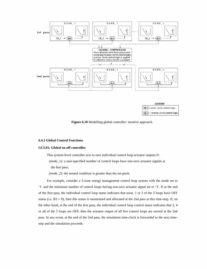
Figure 6.18Modelling global controller: iterative approach.
6.4.3 Global Control Functions
GCL01: Global on-off controller.
This system-level controller acts to zero individual control loop actuator outputs if:
(mode_1):a user-specified number of control loops have non-zero actuator signals at
the first pass;
(mode_2):the sensed condition is greater than the set-point.
For example, consider a 5-zone energy management control loop system with the mode set to
‘1‘ and the minimum number of control loops having non-zero actuator signal set to ‘3‘. If at the end
of the first pass, the individual control loop status indicates that none, 1 or 2 of the 5 loops have OFF
status (i.e. B3 = 0), then this status is maintained and allocated at the 2nd pass at this time-step. If, on
the other hand, at the end of the first pass, the individual control loop control status indicates that 3, 4
or all of the 5 loops are OFF, then the actuator output of all five control loops are zeroed at the 2nd
pass. In any event, at the end of the 2nd pass, the simulation time-clock is forwarded to the next time-
step and the simulation proceeds.

GCL02: Global capacity management controller.
This global controller acts to sequentially zero nominated individual control loop actuator
outputs in order to limit the total system flux capacity to within user-defined limits. Again, after the
1st pass at any given simulation time-step, the individual control loop status values are determined in
the conventional ESP-r manner. The output of all control loops are summed to obtain the system
requirement. If this value is within the specified range, then at the 2nd pass the individual control loop
status values, as computed at the 1st pass, are allocated. If, on the other hand, the system requirement
is outwith the specified capacity limits, then user-defined control loop actuator outputs are zeroed until
the revised system energy requirement is within range.
As an example, consider a 5-loop system. If the user has specified 3 control loops (LOOP_3,
LOOP_1 and LOOP_4) which may be shed to satisfy capacity limits, then the actuator signal for these
loops will besequentiallyzeroed until the revised total system output is within capacity limits. If,
having sequentially switched off (zeroed) all specified loops, the revised system energy requirement
still exceeds capacity limits, then all nominated outputs are zeroed whilst the remaining outputs
maintain their status as computed at the 1st pass.
GCL03: Global sequence controller.
This global controller facilitates the simulation of global phasing strategies. An energy demand
reduction strategy commonly adopted in a BEMS involves individual control loop actuators being
activated with the precondition that nominated control loops have ON status. For example, consider
the following 3-loop control scheme. The user-specified number of scheduled loops may be set to ‘3‘,
with sequence, say: LOOP_3, LOOP_1 and LOOP_2. Thus, LOOP_3 and LOOP_1 output mustboth
be non-zero for LOOP_2 to be activated else LOOP_2 will be zeroed (at the 2nd pass) at this time-
step. A sample control scheme for the 3-loop example is shown in Table 6.9 and Figure 6.19, where
all combinations of sequencing are assessed.
GCL04: Global parameter reset controller.
One of the most common BEMS supervisory control functions is the resetting of local loop
controller set-points in an attempt to reduce energy demand. This global controller acts to
dynamically resetany local zone-level control function (x_fnc) miscellaneous data item, (x_md) to
some user-specified value (x_reset). Any miscellaneous data item may be dynamically reset: set-point,
integral action time, throttling range, offset, etc. This may be extended to conditional reset according
to some sensed variable, as specified by the global sensor definition. The effect of resetting a building
control function set-point according to external temperature is shown in Tables 6.10(a) and 6.10(b)
and Figures 6.20(a) and 6.20(b) (casea for no global control active and caseb for global parameter
reset active). Here, the zone air temperature set-point is reduced from 20°C to 17°C in the event of
the external air temperature falling below 0°C.

GCL05: Global scale and offset controller.
This system-level controller acts - according to a range of global logic conditions - to scale
and/or offset the zone-level controller outputs evaluated at the first pass. Scaling/offset is active in the
event that the (global) sensed condition (mode_1), or rate of change of sensed condition (mode_2),
exceeds the user-specified set-point. This controller allows the modelling and appraisal ofcentralised
trimming control strategies; for example, this global controller may be set up to reduce all/selected
zone-level controller outputs by 30% if the external relative humidity exceeds a given value.
GCL06: Global free-float controller.
This system-level controller should be specified during control periods whereno global strategy
is assumed to be active. No supplementary data items are required.
6.4.4 Modelling system-level controllers - non-iterative approach.
Non-iterative methods for modelling hierarchical MIMO systems are now investigated. An
example of how supervisory control is modelled in an non-iterative manner in sequential type energy
simulation programs, is the TRNSYS TYPE 99 Supervisory Controller for Air Handling Unit (AHU)
and Variable Air Volume (VAV) systems [Corrado and Mazza 1990]. In this supervisory controller
model (Figure 6.21), 42 input variables are obtained from sensors and 28 output variables are sent to
control devices. Modifiable control algorithms include 12 on-off controllers and 11 PID controllers.
A non-iterative approach to the modelling of hierarchical MIMO systems suitable for the
incorporation in the modular, simultaneous, dynamic simulation program, ESP-r, is now presented.
As elaborated in Section 3.3, zone-level building-side control functions are processed, at any given
time-step, in a sequential manner, each subsystem control function operating on the most recently
computed future time-row values. In the non-iterative approach to systems-level controller modelling,
all subsystem controller outputs, at each time-step, are continuously fed to the global controller for
processing (Figure 6.22). Unlike the iterative approach - in which global control logic is applied only
after all zone-level building control functions have been processed at the first pass - this ‘direct‘
method processes all zonal subsystem control functions as they are computed and fed to the global
controller at the first pass. In this way, the control functions are processed in much the same way as
arepractical,multiplexed, cascaded BEMS zone-level control functions, i.e. continual resetting of set-
points, logic parameters, etc.
A global controller model based on this approach is now presented.

Table 6.9: Global sequence controller, control schedule.
Period_1 Period_2 Period_3Control function Associated
type zone Start Law Start Law Start Law
Building 1 00.000 Ideal 03.00 Free-float 05.00 Ideal
Building 2 00.000 Ideal 10.00 Free-float 14.00 Ideal
Building 3 00.000 Ideal 00.000 Ideal 00.000 Ideal
Global All 00.000 Sequence 00.000 Sequence 00.000 Sequence
(a) Sequence: 1-2-3 (b) Sequence: 1-3-2
(c) Sequence: 2-1-3 (d) Sequence: 2-3-1
(e)Sequence: 3-1-2 (f) Sequence: 3-2-1
Figure 6.19Global sequence control.

Table 6.10(a): Control schedule - no active global control.
Control Assoc. Period_1 Period_2 Period_3
Start Type Set-point Start Type Set-point Start Type Set-pointfunction zone
Building 1 00.00 062-001-103 10.0 07.00 062-001-110 20.0 18.00 062-001-110 12.0
Fluid flow 1 00.00 062-002-081 15.0 00.00 062-002-081 15.0 00.00 062-002-081 15.0
Figure 6.20(a)Global set-point reset controller not active.
Table 6.10(b): Control schedule - global set-point reset controller active.
Control Associated Period_1 Period_2 Period_3
Start Type Set-point Start Type Set-point Start Type Set-pointfunction zone
Building 1 00.00 062-001-103 10.0 07.00 062-001-103 20.0 18.00 062-001-103 12.0
Fluid flow 1 00.00 062-002-081 15.0 00.00 062-002-081 15.0 00.00 062-002-081 15.0
Global All 00.00 Free-float - 00.07 009-046-161 00.00 18.0 Free-float -
Figure 6.20(b)Global set-point reset controller active.

Figure 6.21TRNSYS-99 Supervisory controller.
Figure 6.22Modelling global controller: non-iterative approach.

Discharge global controller.
Discharge control of cooling coil with damper sequencing is one commonly adopted BEMS
global control strategy. A schematic diagram of aHoneywell Chiller Discharge Global Controller
[Honeywell 1989] is shown in Figures 6.23(a) and 6.23(b). The system consists of minimum and
maximum outdoor damper air control loops and a cooling valve control loop integrated with an energy
management optimum start control loop. Controller elements include PID (split range) together with
logical AND elements. The global controller receives inputs from the fan differential pressure sensor,
the outside air temperature sensor, the discharge air temperature sensor and the zone air temperature
sensor. Global actuation set-points are the return damper, the maximum outside air damper, the
minimum outdoor air damper and the chiller control valve.
Sequence of Operation.On a rise in discharge air temperature, the discharge air PID operator
modulates the maximum outdoor air damper open in sequence with the chiller valve to maintain the
set discharge temperature. The sequencing ranges (Parameters 6,7,8, and 9) are field adjustable
parameters. Any time the outdoor temperature exceeds the set point, the maximum outdoor damper
closes and the return damper opens.
Optimum start program.When the fan runs (switched on by the optimum start/ occupancy routine,
and indicated by the differential pressure signal), the plant/control system is enabled.
Maximum outdoor damper control.The digital output of the logic operator is 1 any time the outdoor
air temperature is less than Parameter 2. This signal isANDedwith the fan logic signal: a resultant 1
output indicates the damper is under control of the PID operator (top range); a resultant logic 0 sets
the damper to a minimum.
Cooling valve control.When the fan is OFF, the differential pressure from the fan sensor is a logic 0,
which subsequently closes the chiller valve. When the signal is a logic 1, however, the PID controller
(low range) with gain Parameters 3,4 and 5 is in charge of the cooling valve.
Minimum outdoor damper control.The fan signal isANDedwith a true (logic 1) from the optimum
start/occupancy schedule controller; a resultant logic 1 signal opens the damper.
In ESP-r, the following zone-level control loops are required for the discharge global controller
described above.
- One building side controller,BCL06, to couple the plant system to the building
zone.
- Two fluid flow proportional controllers,FCL01, one for the return/ maximum air
damper and one for the minimum outside air damper.
- Two plant controllers:PCLO4 for the plant optimum start routine andPCLO2 for
the PI chiller control.

The zone-level control loop sensed values and actuator outputs are fed, at each time-step, to the
global chiller discharge control function,GCL05, which orchestrates the control according to the
global control logic strategy outlined above by establishing appropriate actuator signals for
subsequent processing by the zone-level controllers. Zone-level control loop sensors and actuators are
specified as usual (Section 3.5) with regard to element location and operational variables; however, in
the case of the customised, ’specific’ global controller described here, the actuator outputs forFCL01
andPCLO2are established byGCL05.
In order to demonstrate system-level discharge global control, consider the test zone controlled
according to the schedule listed in Table 6.11. The global function attempts to maintain the zone air
point temperature within the range 18-22°C for the occupancy period, 09.00-18.00 hours. Figure 6.24
shows the global controller input/output signals for a 1-day simulation period run with building-side
and plant-side time-steps of 6 minutes and 60 seconds, respectively. Note that scalar offsets on the
results plots are used for clarity and also that time-step averaging is disabled.
As expected, prior to the optimum start signal being received, the global controller acts to close
both minimum and maximum outdoor air dampers and to disable the PID controller. Upon reaching
the predicted start-up time of 05.50 hours, the minimum damper opens fully and the maximum
outdoor damper modulates open for a short time until the chiller operates and/or the outdoor dry bulb
temperature exceeds the pre-set value of 22.5°C at which stage it closes as described earlier. The PID
controller output (proportional mode only in this case) is oscillatory; this is a function of the
simulation time-step and also the specified proportional bands. (It is also due in part to the time-step
averaging of results being disabled). Further tuning could expect to achieve smoother profiles.
However, the overall performance of the controller is shown to be satisfactory, the (averaged) zone air
temperature generally being held within the specified tolerance band during the period of occupancy.
Clearly, the success of such a modelling technique may often be dependent on the simulation
time-step. It is likely that, in attempting to model reality and capture the dynamics of practical
building/plant/control systems, a (relatively) small time step will often be required for the building
and plant-side time-steps; of the order of 6 minutes and 1 minute, respectively, possibly reducing to 1
minute and 6 seconds in some cases, e.g. for heat exchanger control loops. No rigid guidelines/rules
can be offered in this respect: often a combination of a knowledge of the expected plant/control
system characteristics and behaviour, a simulationist’s experience and adoption of iterative, trial-and-
error procedures, are required in order to determine suitable time-step values. Possibly the best way of
establishing appropriate time-steps is to ascertain the polling rate employed in a practical BEMS. This
can, however, prove to be problematic, considering the reluctance that many plant/control system
manufacturers have to publishing representative performance data [Aasem 1993].

Figure 6.23(a)Chiller discharge global controller schematic [Honeywell, 1989]
Figure 6.23(b)Chiller discharge global control logic [Honeywell, 1989]

Table 6.11 Global discharge controller: control schedule.
Parameter 1 2 3 4 5 6 7 8 9 Occupancy Set
(Fig 6.25(b)) Ambient temp. limits PID gains Sequence limits period point
22.5°C 22.5°C 25.0 0.0 0.0 -20.0 12.0 12.0 40.0 09.00-18.00 18-22°C
Figure 6.24Chiller discharge global control: sample results set.

6.5 IMPLEMENTATION OF CONTROL FUNCTIONS IN ESP-r.
The zone-level and system-level controller models installed in ESP-r, and described above, may
be supplemented by additional models as the modelling need requires. For this reason, the following
set of guidelines for implementation of control functions in ESP-r are now presented. The
recommended procedure involves 8 stages (Figure 6.25):
- Stage 1. Deciding on the control function (practical or imaginary) to be modelled;
- Stage 2. Construction of a flow-chart indicating the main stages in the control logic;
- Stage 3. Coding the algorithm in the FORTRAN-77 programming language;
- Stage 4. Installing the coded algorithm in the relevant control subsystem module(s);
- Stage 5. Possibly updating the moduleMakefile;† to include any subroutines and/or
functions contained in new file(s), for subsequent program compilation;
- Stage 6. Code checking, debugging and performance testing the coded algorithm to
ensure numerical integrity with the entire program system (These issues are
elaborated in Chapter 7);
- Stage 7. Development of graded tutorial exemplars suitable for subsequent use by a
wide group of users, ranging from novice simulationists through to expert users and
model developers;
- Stage 8. Updating the interface to allow user definition and specification.
The control functions themselves should have the necessary code required to:
- prohibit an incorrect number of controller defining data items being specified;
- provide range checks on the controller defining data items, and thus guard against
‘silly‘ data input;
- prevent division by zero;
- issue warnings should unrealistic control system data be computed.
† make is a UNIX program which reads a specification (held in amakefile) of how the components of a programdepend on each other, and how to process them to create an up-to-date version of the program. It checks the times at whichthe various components were last modified, figures out the minimum amount of recompilation that has to be done to makea consistent new version, then runs the processes.

Figure 6.25Implementation of new control functions in ESP-r.

6.6 SIMULATION ASSISTED CONTROL.
6.6.1 Basic concept.
The zone-level and system-level controller models described above, offer the possibility of
modelling a vast range of both practical and highly conceptualised control system types. Simulation,
however, need not be restricted to such research and design applications: there exists the very real
possibility of extending its use by employing energy simulation programs on-line in BEMS, to act in
the role of an intelligent control supervisor.
The notion of marrying the two technologies is supported by BEMS multiplexing techniques
which allow rapid, on-line adjustment of control system parameters on the basis of simulated
forecasts. Simulation provides a look-ahead capability which facilitates predictions of future reality
which can then be used to determine the best possible control action in terms of comfort and energy
levels (Figure 6.26). Simulation time-step controllers (described in Section 5.3.4) can then be invoked
which enable trial (present) control actions to be simulated in rapid iterative mode until the controller
performance is deemed to be satisfactory/optimised (in terms of predicted future outcomes) at which
point the simulation proceeds to the next control period. The optimised control system parameters
may then be implemented in the BEMS.
As explained in Section 2.2, modern-day practical controllers are often based on acontroller/
system modelstructure. The premise implicit with the simulation-assisted control concept is that there
is no need for separate system model generation (e.g. by employing identification methods), since in
this case the system model is held in the form of system matrix, as described in Chapter 3. Clearly,
this results in a simplification of the control system synthesis process, offering, for the first time, the
opportunity for building design professionals - not necessarily familiar with highly esoteric control
engineering theory - to participate in system design and operation.
The design and operation of practical building control system logical elements requires the
following.
(1) A defined objective: control theory concerns itself with the future state of the
system. The objective of any control system in every case is connected with the
performance of the system over some period of time.
(2) A choice of possible control actions: if no variation of actions is possible, control
is not possible since the course cannot be modified.
(3) A means of choosing the correct control strategy. Thus a model of the system is
required which is capable of predicting the effect of various control actions on the
system state.
The concept ofenergy simulation assisted control decision making(ESAC) offers a means by
which these requirements may be met, during both the design and operation of BEMS. The main

advantages of a simulation-assisted approach to control design/operation are as follows.
- Any criterion whatever can be used for the decision process, e.g. there is no need to
be restricted to, say, quadratic criteria as in conventional optimal control design.
- The difficult and highly specialised problem of control synthesis is avoided.
- Control actions can first be appraised in a software environment before being
applied to the real system. This feature offers tremendous potential for the next
generation of intelligent buildings and BEMS.
Figure 6.26Energy simulation assisted control
6.6.2 ESAC algorithms.
Situations where energy managers could employ predictive-iterative simulation schemes are
numerous, and include optimisation of:
- plant system start/stop times;
- set-back temperatures;
- sensor/actuator location/variable;
- control mode (fuzzy logic, multi-stage, etc);
- flux injection/extraction levels;
- duty cycled plant components and cycling periods;
- load shedding schema;

- fluid flow network balancing.
The development of ESAC algorithms for such applications are now described. The schemes
presented employ the simulation time-step controller (TSCON_8), described in Section 5.3.5, to reset
the simulation time-clock and thus facilitate iteration.
ESAC01: ESAC optimum start/stop.
Almost all BEMS will have a number of microprocessor-based optimum start/stop control loops
available for use. The purpose of the algorithm is to relate the time required for preheat (lead time) to
the observed building and/or outside temperatures: equipment is started to ensure the achievement of a
comfort level when the first occupant arrives; equipment is stopped when comfort levels can be
maintained until the last occupant leaves. Energy savings of up to 40% may be achieved as compared
with switch-on by timer [Kohonen, 1984].
There are two main classes of optimum start/stop algorithm: empirical and theoretical.
Empirical and semi-empirical optimisers (e.g. the Birtles and John algorithm of thePCL04 control
function, discussed in Section 6.3.2) are based on an observed or assumed relationship between the
preheat time and temperatures.
More recently, self-tuning optimum start controllers have been proposed [Murdochet al 1990].
These controllers have their parameters continually updated as the BEMS observes the performance of
the controller. The associated algorithms are based on semi-empirically derived relationships between
the preheat time and the bulk temperature of the zone to be controlled. Such controllers are claimed
not to require any prior knowledge of the thermal characteristics of the heating plant and building. The
bulk temperature is based on the variables related to the characteristics of the building and outside
temperature as predicted using a first-order model of the room and heating plant. One of the main
reasons for serious performance deficiencies in commercially available optimisers is poorly designed
optimiser schedules and inefficient self-learning procedures, which are incapable of accurately
reflecting the thermal response of buildings [John and Smith 1987].
A proposed new approach for design and/or on-line BEMS applications, is to develop an ESAC
algorithm to determine the optimum start-up and optimum shut-down times of the building plant
system. Using the numerical method described in Section 3.3, in which the system matrixis the
building/plant model, simulation can be used in rapid iteration mode to accurately predict the
controlled start/stop times. The method is depicted in Figure 6.27. Trial times are predicted and used
in the simulation for any specified control period (day, week, month, season, etc.). Zone air
temperatures at the ‘desired time of arrival/departure‘ (DTOA/D) can then be predicted. If trial times
result in satisfactory air temperatures at the DTOA/D, then the trial times are accepted and the
simulation proceeds to the next time-step. If, on the other hand, the trial times are not acceptable, then
once all zones have been processed at that time-step, an iterative scheme is activated by which the

simulation time-clock is reset to the start of the control period by means of the simulation time-step
controller (TSCON_8), and the system matrix reconstructed toexactly the same coefficients as the
previous pass at this time-step. At this point, new trial times are predicted using a binary search
algorithm to forward/retard the trial times according to results at the previous pass, and then a further
simulation for the control period commences. This prediction-iteration process continues until
satisfactory control performance is achieved after which the simulation proceeds to the next control
period.
Controller models based on the above approach are installed in ESP-r. Figure 6.28 shows a
sample result set for controllerBCL15applied to a single zone.
Figure 6.27 ESAC optimum start schedule.

Figure 6.28 ESAC optimum start results.
ESAC02: ESAC optimum set-back temperature.
Set-back of temperatures during periods of nonoccupancy is another commonly adopted
intermittent heating control scheme. Here, for the period of nonoccupancy, the set-point is decreased
to an acceptable minimum; a value determined after taking into account factors such as energy
demand and frost protection of building fabric/contents. Typically, this value is fixed for the duration
of the control period. Since a fixed set-back temperature for the duration of the control period may not
maximise plant system efficiency, it may be deemed more appropriate in some instances to fix the
plant capacity and vary the set-back temperature, with some limiting value for frost protection.
Simulated-assisted control can be employed to search for the lowest possible set-back temperature,
taking due account of any user-specified criterion. This scheme is depicted in Figure 6.29(a).
Consider a single zone controlled according to the following schedule: ideal control (set-point
of 21 °C) for the period of occupancy (08.00-01.00 hours); and one period of nonoccupancy (01.00 to
08.00 hours) with the set-back temperature to be determined. During the set-back period, the
controller at each simulation time-step iteratively searches for the lowest set-back temperature
possible given a limiting period cumulative load capacity constraint, and a minimum frost protection
temperature level (10°C). The results for this control scheme for a two week period in early January,
are shown in Figure 6.29(b) from which the time-varying temperature set-back levels can be seen.
The simulation period iterations are shown in Figure 6.29(c).

Figure 6.29(a)ESAC optimum set-back temperature: trial set-backs.
Figure 6.29(b)ESAC optimum set-back temperature: sample results set.
Figure 6.29(c)ESAC optimum set-back temperature: numerical iterations.

ESAC03: ESAC sensor/actuator location.
BEMS normally control on the sensed condition as monitored at fixed positions throughout the
network. Similarly, BEMS actuation points are typically unchanged for the duration of the control
period. It is possible, however, to envisage a situation whereby energy managers - with the aid of on-
line energy simulation tools - can forecast system conditions resulting from control on amultitudeof
sensor and/or actuator locations/variables. For example, energy managers may assess, in advance of
implementation, the outcome of the following strategies.
- Controlling on dry bulb air temperature as opposed to controlling on dry resultant
temperature.
- Actuating at air point, specified surfaces or intra-constructional points.
- Varying the convective/radiative ratio for sensor and/or actuator signals.
In the ESAC03 controller,TSCON_8 is utilised to iteratively search for the optimum
location/variable in terms of some specified criterion, say energy requirements or comfort levels. Once
all options have been assessed, the simulation proceeds to the next control period.
The results for various surface sensor locations for a single zone problem are listed in Tables
6.9-6.11, where the optimum sensor location is decided on the basis of a variety of criteria for the
control period, namely (a) lowest cumulative energy demand, (b) lowest mean energy requirements
and (c) lowest period peak demand.
The results for a range of convective/radiative ratios for both mixed sensor and mixed actuator
control are shown in Figures 6.30 and 6.31, respectively, where the effects (in terms of load) for
various ratios are clearly seen.
ESAC04: ESAC control mode optimisation.
As with practical sensor and actuator elements, the control mode in a BEMS is usually pre-set
for the different control periods. Again, however, it is possible to invoke simulation-assisted control
schema in an attempt to optimise system efficiency, by iteratively searching (usingTSCON_8) for the
control law which offers the best performance in terms of a vast range of operating criteria.
A sample results set for a control mode (law) optimiser applied to a single zone problem are
shown in Figure 6.32. Here, three control modes (ideal, fixed input/extract and two-position) are
iteratively assessed over the same control period, the optimum mode established (in terms of, say,
deviation from the set-point of 20°C), at which juncture the simulation proceeds to the next control
period.
An option with this simulated-assisted controller is to iteratively adjust some controller
parameter (e.g flux capacity, throttling range, set-point, integral action time, etc.) and forecast building
environmental performance. The results for iteratively adjusting controller flux capacity in the case of
BCL04 fixed injection/extractioncontroller mode, are shown in Figure 6.33.

Table 6.9: Simulation-assisted sensor location: criterion (a)
Energy performance Control OptimumDay
Number Lowest cum. demand Lowest swing Min. peak demand Lowest mean criterion location
1 Surface_3 Surface_3 Surface_4 Surface_4 Lowest cum. demand Surface_3
2 Surface_4 Surface_4 Surface_3 Surface_4 Lowest cum. demand Surface_4
3 Surface_1 Surface_1 Surface_4 Surface_4 Lowest cum. demand Surface_1
4 Surface_3 Surface_3 Surface_2 Surface_4 Lowest cum. demand Surface_3
5 Surface_1 Surface_1 Surface_4 Surface_4 Lowest cum. demand Surface_1
6 Surface_3 Surface_3 Surface_2 Surface_4 Lowest cum. demand Surface_3
7 Surface_2 Surface_2 Surface_3 Surface_4 Lowest cum. demand Surface_2
Table 6.10: Simulation-assisted sensor location: criterion (b)
Energy performance Control OptimumDay
Number Lowest cum. demand Lowest swing Min. peak demand Lowest mean criterion location
1 Surface_3 Surface_3 Surface_4 Surface_4 Lowest mean demand Surface_3
2 Surface_4 Surface_4 Surface_3 Surface_4 Lowest mean demand Surface_4
3 Surface_1 Surface_1 Surface_4 Surface_4 Lowest mean demand Surface_4
4 Surface_4 Surface_3 Surface_2 Surface_4 Lowest mean demand Surface_4
5 Surface_1 Surface_1 Surface_3 Surface_4 Lowest mean demand Surface_4
6 Surface_4 Surface_4 Surface_1 Surface_4 Lowest mean demand Surface_4
7 Surface_4 Surface_4 Surface_1 Surface_4 Lowest mean demand Surface_4

Table 6.11: Simulation-assisted sensor location: criterion (c)
Energy performance Control OptimumDay
Number Lowest cum. demand Lowest swing Min. peak demand Lowest mean criterion location
1 Surface_3 Surface_3 Surface_4 Surface_4 Lowest peak demand Surface_4
2 Surface_4 Surface_4 Surface_3 Surface_4 Lowest peak demand Surface_3
3 Surface_1 Surface_1 Surface_3 Surface_4 Lowest peak demand Surface_3
4 Surface_4 Surface_3 Surface_2 Surface_4 Lowest peak demand Surface_2
5 Surface_1 Surface_1 Surface_4 Surface_4 Lowest peak demand Surface_4
6 Surface_3 Surface_3 Surface_2 Surface_4 Lowest peak demand Surface_2
7 Surface_2 Surface_2 Surface_4 Surface_4 Lowest peak demand Surface_4
Figure 6.30ESAC mixed convective-radiative sensor control.

Figure 6.31ESAC mixed convective-radiative actuator control.
Figure 6.32ESAC control mode optimiser.

Figure 6.33ESAC controller output optimiser.
ESAC05: ESAC duty cycling.
Load balancing, by means of duty cycling, is a classical optimisation/allocation problem
typically solved using linear programming techniques involving cost functions, constraints, and
equalities/inequalities: such problems come within the realms ofOperational Research[Taffler 1979].
The scheme presented here is a simulation-assisted approach to solving the problem of establishing
optimum cycle schedules. (A model for a conventional duty cycle controller,PCL07, was described in
Section 6.3).
Each plant component is specified in terms of its power rating. The objective function
represents the total energy of the system, and the constraints are the minimum and maximum on times
for each component. The problem becomes one of minimising the total system energy demand whilst
satisfying the specified constraints. Consider the cost function,
E = w1e1 + w2e2 + w3e3. . . . . . .+wnen (6.57)
wheree is the plant energy demand (i.e. power rating x cycle period) andw is the status of plant
component (0 = off; 1= on). This objective function may also be liable to constraints. For example,
component1 may be subjected to the constraint that it is on for a minimum of 20% and a maximum of
80% of the duty cycle period whilecomponent2 may be constrained so that it is on for a minimum of
20% and a maximum of 95% of the duty cycle period. The problem is to minimiseE given the
constraints onw. A minimisation can be achieved by maximising the negative of the objective
function. So-called ‘slack variables‘ are added to turn the inequality constraints into equalities.

A possible procedure is as follows.
Stage 1Specify power rating for all duty cycled plant, n,Pi , (i = 1 to n)
Stage 2Specify time base, T.
Stage 3Evaluate energy from:
ei = Pi T. (6.58)
Stage 4Specify cost function to minimise - in this case the sum of squared plant energies:
J = w21e2
1 + w22e2
2 + w23e2
3+. . . .w2ne2
n =n
i=1Σ w2
i e2i (6.59)
wherew1, w2, etc, represent values of 0 or 1 to indicate if the supply is being used.
Stage 5 (a) Apply quality constraints.For example, the output load at any time-step is required to be
Y:
n
i=1Σ wi ei = Y. (6.60)
Stage 5(b) Apply inequality constraints.For example, over a time period,N x T (where N is the
number of plant-side time-steps per duty cycle period,T) ei is required to be on for less thanNmax
time-steps, i.e.
N
i=1Σ ei wi ≤ eimax (6.61)
where
eimax = Pi NmaxT. (6.62)
This states thatei must be on for less thanNmax time-steps during the lastN time-steps. For example,
if T is 1 minute,Nmax is 30 time-steps andN is 60, thenei must be on for less than 30 minutes. It may
also be the case thate1 must be on for only (say) 40% of the total load, hence:
40%=Nmax
Nx100 (6.63)
Therefore, ifN is 60 minutes,Nmax would be 24.
Stage 6Include in cost functions.
J1 =n
i=1Σ(wi ei )
2 + λ1
n
i=1Σ(wi ei − Y) (6.64)
J2 =N
k=1Σ Jk + λ2(
N
i=1Σ(wi ei + α i − eimax)) (6.65)
whereλ is a scalar function of the controlled variables andα i is a ‘slack variable‘ to allow inequalities
to be written as equalities.

At the end of each control period, the simulation has established on-off periods for each plant
item based on the specified constraints. However, in order to find the optimum duty cycling scheme, in
terms of which plant to cycle and under what restraints, the simulation time clock can be reset (by
means ofTSCON_8) to the start of the control period, and a new minimum energy demand calculated
for a different set of plant items and/or constraints.
ESAC06: ESAC load shedding algorithm.
Unlike most other BEMS functions, load management by load shedding, is designednot to
reduce energy consumption but to reduce maximum demand penalty charges and to alleviate the peak
demand on utilities. If the kW electrical demand goes too high in any half-hour in the month, then the
user has to pay for this worst half-hour in the month. It is therefore worthwhile to keep the maximum
demand at a low and steady level. Various methods of load shedding are discussed by Levermore
[1992].
The ESAC algorithm, described below and depicted in Figures 6.34 and 6.35, monitors the
cumulative demand for any specified demand interval and compares the forecast demand to the
allowable value and, if necessary, shed loads on either a time or size basis.
The procedure is as follows.
Stage 1At the start of each demand interval (DI), the cumulative consumption
(DCC) is re-initialised to zero.
Stage 2At the end of the DI, the DCC is compared with the target cumulative
consumption (TCC). If the DCC is less than, or equal to, the TCC then simulation
proceeds to the next DI. If, on the other hand, the DCC is greater than the TCC then
the following predictive-iterative procedure is invoked.
Stage 3Time-step controllerTSCON_8is invoked to reset the simulation time clock
to the start of the DI.
Stage 4Loads are shed according to the specified priority criteria.
Stage 5A further simulation is run using the revised plant group on/off status values;
Stage 6 Stages3-5 are repeated until DCC is less than, or equal to, TCC.
With the ESAC06controller, shedding can be done on either a group or a time-step priority
basis. If the former, then at each reset operation and at the same simulation time-step, group loads are
shed in increasing number. If the DCC is still too high when all specified groups have been shed, then
the simulation time-step is decremented by unity, and groups are shed in increasing number at this
simulation time-step; and so on until the DCC is within the required range. If, on the other hand, the
shedding process is on a time-step basis, then the number of groups shed is fixed for each simulation
reset as each DI time-step is passed through. If the simulation time-step has reached as far back as the
first time-step and the DCC is still too high, then the groups shed are incremented by one group and
the simulation time-step backward stepped at subsequent simulations.

Figure 6.34ESAC load shedding algorithm flow chart.

Figure 6.35ESAC load shedding algorithm: shedding priority.
ESAC07: ESAC balancing controller.
Tuning and commissioning controllers is as problematic in simulation as it is in practice. BEMS
suppliers are increasingly using sophisticated software tools to speed up and improve the quality of
system design and commissioning. This section describes how simulation can assist the
commissioning of fluid flow networks.
Design engineers aim to balance the fluid flow circuits at the design stage of a project so that,
when the systems are brought into operation, each outlet or unit will operate at the design flow rate,
within specified tolerances. Devices for regulating the flow in the ductwork and pipework systems
then exist to allow on-site balancing such that each outlet or unit receives its rated flow rate. However,
in practice, many systems are operated in either an unbalanced state, with the resulting loss of plant
system efficiency, uncomfortable zonal air movement patterns, and incorrect temperature and
humidity conditions. Several studies have shown the importance of good commissioning procedures
for building energy performance. For example, a study of the benefits of retrofitting BEMS in existing
buildings [John and Smith, 1987] revealed that most of the considerable savings were found to be
attributable to the recommissioning of the HVAC plant control systems.
Poorly commissioned plant is due, in part, to the fact that balancing a flow system typically
involves very time-consuming and tedious trial and error commissioning procedures. This is
particularly so in cases where the valve/damper sets are physically remote from one another (e.g. on
different floors), often requiring the commissioning engineers to cover large distances between trial
adjustments. Consequently, such procedures are often neglected or carried out in an unsatisfactory
manner.
One way of addressing this problem is to use fluid flow simulation to predict the optimum
valve/damper settings for the flow network branches such that a balanced system exists. The ESAC
flow network balancing algorithm now described is based on the balancing method proposed by
Harrison and Gibbard [1965] and adopted by the CIBSE Commissioning Codes for air and water
distribution systems (Series A [1971] and Series W [1989], respectively).
The procedure (which may be carried out at all/selected time-steps) is as follows.
Stage 1: Preliminary checks are made in the program to ensure that all
valves/dampers in all the specified branches are set to 100% open.
Stage 2:The ratio of measured flow rate to the design flow rate,R, is computed for
each branch.
Stage 3:The index line (i.e. the branch having the smallestR ratio in any group of
outlets served by a branch) is established for each branch with all valve/dampers
open.
Stage 4:Each branch line valve/damper is (iteratively) adjusted in order of increasing
R ratio, such that all the lines receive their correctproportionof the total flow rate.

Stage 5:Design branch flow rates at Stage 4 are unlikely, and branch fan/pump
and/or supply valve/damper adjustment is usually necessary to ensure that the
branches receive their design flow rates within a specified tolerance of balance.
This procedure, then, may be employed (on-line on a BEMS) to give a time-series of percentage
valve openings as required for balanced flow networks.
A number of schemes for modelling building control systems logical elements have been
presented in this chapter including zone-based and systems-level control structures and also the
concept of simulation-assisted control. The following chapter proceeds to discuss issues relating to
validation of the developed schemes.
References.
Aasem, E.O., 1993. ’Practical simulation of buildings and air conditioning systems in the transient
domain,’Ph.D Thesis,University of Strathclyde, Glasgow.
BEMS Centre, 1988.DLP2: Control with a building energy management system,BSRIA, Berkshire,
U.K.
Birtles, A., and John, R.. ’A new optimum start algorithm’,Building Services Research Engineering
Research and Technology’,Vol. 6 No. 3. (1985).
Bristol, E.H., 1977. ’Designing and programming control algorithms for DDC systems’,Control
Engineering, pp. 24 - 26.
CIBSE Guide A.1. Environmental criteria.CIBSE, Balham, London (1979).
CIBSE Commissioning Code: Series A,Air Distribution, Chartered Institution of Building Services
Engineers, 1971.
CIBSE Commissioning Code: Series W,Water Distribution, Chartered Institution of Building
Services Engineers, 1989.
Clark, D.W. 1985. ’PID algorithms and their computer implementation’,Transactions of the Institute
of Measurement and Control,Vol 6, No 6: pp. 305-316.
Clarke, J. A., 1985,Energy Simulation in Building Design, Adam Hilger Ltd, Bristol UK.
Corrado, V., and Mazza, A., ’Supervisory Controller Component’,IEA Annex 17 Report,Politecnico
di Torino, Italy, Feb. 1990.
Dexter, A.L., ’Control systems computer control’,Energy and Buildings,Vol. 10, pp. 203-211, 1988.
Harrison, E., and Gibbard, N.C., ’Balancing air flow in ventilating duct systems’,Journal of Institute
of Heating and Ventilating Engineers,, Vol. 33, 1965, p. 201.
Haves, P., and Dexter, A.L., ’Simulation of Local Loop Controls’,Proc. Building ’89, IBPSA
Vancouver, June, 1989.
Hensen, J.L.M. 1991. ’On the thermal simulation of building structure and heating and ventilating
system’,Ph.D. Thesis,Technische Universiteit, Eindhoven.

Honeywell,Engineering Manual of Automatic Control,Minnesota: Honeywell, Inc., 1989.
Isermann, R.Digital Control Systems,New York: Springer-Verlag, 1981.
Jamshidi, M., Nader, V., Ross, T, J. 1993.Fuzzy Logic and Control - Software and Hardware
Applications.Prentice Hall, New Jersey, U.S.A.
John, R.W., and Dexter, A.L., ’Intelligent controls for building services’,Building Services Research
Engineering Research and Technology’,Vol. 10, No. 4, pp. 131 - 141 (1989).
John, R.W., Smith, G.P, 1987 ’Operating experience of building management systems’,Proceedings
of ICBEM 1987: The International Congress on Building Energy Management,Lausane,
Switzerland.
Jones, W.P. 1985.Air Conditioning Engineering,Arnold, London.
Kelly, N.J., 1997.’Ph.D Thesis (to be submitted)’,ESRU, University of Strathclyde, Glasgow.
Kohonen, R., ’Intermittent Heating of Buildings’,Proc. CIB-W79 Conf. Performance of HVAC
systems and their controls in buildings,Garston, UK (June 1984).
Levermore, G.J., 1992.Building Energy Management Systems,Spon, London.
McCauley, J.J., ’Fuzzy Logic Torque Servo’,The C Users Journal,March, 1994.
Murdoch, N., Penman, J.M., and Levermore, G.J., ’Empirical and theoretical optimum start
algorithms’,Building Services Engineering & Research Technology,Vol. 11, No. 3 pp. 97-103
(1990).
Nakhi, A., 1995. ’Adaptive Construction Modelling Within Whole Building Dynamic Simulation’,
Ph.D Thesis,University of Strathclyde, Glasgow.
Negrao, C,. 1995. ’Conflation of Computational Fluid Dynamics and Building Thermal Simulation’,
Ph.D Thesis,University of Strathclyde, Glasgow.
Ogata, K.Discrete-time control systems,New Jersey: Prentice-Hall, 1987.
Scheepers, H.P.,Inside Building Energy Management Systems, Uitgeverj De Spil Bv, Woerden, 1991.
Taffler, R.Using operational research - a practical introduction,Prentice-Hall, London, 1979.
Tang, D., 1985, ’Modelling of Heating and Air Conditioning System’,PhD Thesis,ESRU, University
of Strathclyde, Glasgow.
Tong, R.M., 1977 ’A Control Engineering Review of Fuzzy Systems’,Automatica,Vol 13, pp.
559-569.
Ziegler, J., and Nichols, N.B, 1942. ’Optimum settings for automatic controllers’,Trans. ASME,Vol.
64, pp. 759 - 768.

Chapter 7
VALIDATION.
This Chapter deals with the issue of software verification of the schemes developed
as part of this project and described in earlier chapters. The main sources of
modelling error and methods for the validation of the developed schemes are
discussed.
7.1 INTRODUCTION.
7.1.1 The need.
During the modelling and program development process, many assumptions and compromises
are inevitably made and, as a result, the exact replication of reality is not achieved. Thus,
industrialists, model developers, practitioners and researchers all have to concern themselves with
issues of accuracy and applicability. As the use of simulation programs has grown over the past 15
years, so designers have come to rely on them to provide accurate results. In trying to guarantee
acceptable performance, designers are being expected to carry out performance assessments which are
beyond the capacity of traditional manual techniques. It is vital, therefore, that designers can trust a
program’s results and, whilst it is accepted that theperfect simulation model is unattainable, it is
nevertheless important that programs are at least accurate enough for the results to fall within an
acceptable margin of error.
7.1.2 Sources of error.
The overall accuracy of simulation programs depends on many factors. Judkoffet al [1983]
identified the main sources of inaccurate predictions in building simulation programs:
- differences between actual and assumed weather conditions;
- differences between actual and assumed occupancy behaviour;
- user error in creating simulation input files;
- differences between actual and assumed thermophysical material properties;
- differences between the actual heat and mass transfer mechanisms and the
algorithmic representation of those mechanisms in the program;
- incorrect software implementation.
Accepting this categorisation of error sources, the first four may be considered asexternal
sources of errors as they are independent of the working performance of the program. The other two
categories are classified asinternal sources since they are under control of the developer and are
directly responsible for the internal program operation. Some of the external sources of errors can be
eliminated by the use of a knowledge-based interface which checks that the input parameters are

within a legal range and supplies intelligent defaults. However, most errors are outwith the
developer ’s control and depend on the user’s judgment, skill and experience in selecting, for example,
boundary conditions. The assumptions made in the running of the program are clearly vital and any
shortcomings in the data input will compromise the accuracy of the simulation. In this respect, it
helps if a user has some hypothesis about the results prior to running the program.
Bowman and Lomas [1985] and Lomaset al [1994], identify some specific examples of internal
sources of error: physical phenomena not included in the modelling because they are thought
(incorrectly) to be unimportant; approximation of relevant complex phenomena; simplification of
physical processes to ease or speed up calculations. Errors on the model derivation, such as unit
conversions, can be added to this list. Simplification involves the adoption of a computer model which
may not be appropriate for the representation of the mathematical devices (such as discretisation
techniques, relaxation factors, linear equation solvers, etc.), although they may be the best approaches
possible.
7.1.3 Approaches to validation.
Practitioners are mainly concerned withoverall program simulation result accuracy.
Researchers, model developers, and program authors, on the other hand, are usually also concerned
with the integrity of individual component, subsystem, and system models (the model validation
process being simpler at component or sub-component level than at whole system level [Chow 1995]).
In any case, quality of prediction tools can be improved via three main approaches. First, by
developing new mathematical models for the better representation of the heat and mass transfers and
the control system characteristics occurring within the building/plant system. Second, by increasing
the simulation resolution in order to reduce the number of simplifying assumptions. Third, by
elaborating a comprehensive validation methodology which includes all the stages of program
development and which may subsequently be deployed in order to determine the range, validity and
the uncertainty of building energy simulation programs. In order to increase the modelling
confidence, it is now widely recognised by researchers that this can only be achieved by repeated
application of a validation methodology by which the programs are exercised in ways which represent
the expected range of application and which are appropriate to the domain of its intended use [Irving,
1988]. One complete validation procedure was developed within the PASSYS project [Jensen 1994]
and comprises the following steps.
- critical evaluation of the theory;
- checking of the source code;
- sensitivity and statistical analysis;
- analytical validation;
- inter-program comparison;
- empirical validation.

Review of theory serves two important purposes: firstly, to understand the scope of an
algorithm; and secondly, to check its coding implementation. As regards source code verification,
during the developments reported here, the code was created using CASE tools (for syntax error
trapping) and debugging tools (for logic error trapping):
forchk is a Fortran program development aid developed at Leiden University. It
verifies the syntax, composes cross reference tables of constants, labels, variables,
arrays, referenced subprograms, and indicates how these items are used. As an
option, forchk validates the syntax for conformance with the ANSI Fortran 77
standard. The reference structure of subprograms can be presented, and cross
reference tables of subprograms, commons, input/output and include files are
composed. Arguments of referenced subprograms and common blocks are checked
for consistency. Cross reference tables of all elements of each common block can be
generated.
dbx is an interactive, line-orientated, source-level, symbolic debugger. It allows the
user to determine where the program crashed, to view variables and expressions, set
breakpoints in the code, and run and trace a program. In addition, machine-level
and other commands are available to help debug the code.dbxtool is a window-
based interface todbx for use onSUN workstations allowing a more convenient
interface. Debugging is easier because the mouse can be used to enter commands
from redefinable buttons on the screen.
A sensitivity analysis is usually concerned with the influence of input parameter variations on
simulation predictions. This is rarely a trivial exercise: for example, the ESP-r system contains
hundreds of variables and parameters which make it virtually impossible to rigorously test the effect
of changing each parameter in a particular situation.
The analytical solution is usually free of uncertainties but its application is restricted to simple
cases. In such cases, it is the most suitable for validating codes related to the specific processes in
isolation since acceptable overall simulation accuracy does not necessarily mean acceptable accuracy
for all processes in isolation. Analytical tests may be used to measure the effect of discretisation and
roundoff errors on the algorithm and its boundary conditions. Theoverall potential of the model under
investigation cannot, then, be checked using analytical validation because only tests for simplified
sub-sets can be analysed. However, these are usually the onlytruth standard available to corroborate
simulation predictions.
In the inter-program comparison approach, a component or system is modelled using different
simulation programs and their predictions compared. Any level of complexity can be tested and no
input uncertainties are present. However, a standard of absolute correctness cannot be identified and
the method fails to give an indication about either the accuracy of a given model or the possible
source(s) of the observed differences.

From a researcher’s point of view, empirical validation is often considered to be the bottom-line
test [Bunn 1995]. Traditionally, this procedure is enacted by comparing the predictions from the
program with corresponding monitored data. Higher accuracy and reliability can be expected provided
that the measurements are accurate. However, application difficulties are often encountered including
the complexities and costs associated with monitoring and extrapolating from specific test conditions
to more realistic cases.
The following sections describe a series of analytical, inter-model and empirical validation tests
carried out in order to verify the control system models installed in ESP-r during the course of this
project.
7.2 VALIDATION TESTS.
7.2.1 Introduction.
It is not possible, given the time constraints of the present work, to test and verifyall the
developed schemes described in earlier chapters, and thus a selection of representative cases will be
considered. In the validation tests reported here, zone-level building, plant-side and global controller
models are assessed. Actuator and sensor delay models are also examined. Table 7.2.1 summarises the
validation test series.
Table 7.2.1 Validation exercises: summary of test series.
Reference Method Controlled system Disturbance Control mode Control function
A1 Analytical Zonal convective heating set-point change Modulating (PID) Building:BCL05
A2 Analytical DHW calorifier Load & set-point change Modulating (PID) Plant:PCL01
B1 Inter-model Zonal convective heating set-point change Intermittent (2-position) Building:BCL10
B2 Inter-model DHW calorifier Load & set-point change Intermittent (2-position) Plant:PCL08
B3 Inter-model Zonal convective heating set-point change Intermittent (Supervisory) Global:GCL03
C1 Empirical AHU chiller set-point change Modulating (PI) Plant:PCL02
7.2.2 Validation test A.1: Analytical validation of building-side controller.
Validation test series A1 involves the analytical validation of the ESP-r building-side
proportional+integral (PI) flux/temperature controller function,BCL05. The simulated results for a
controlled convective heating system are compared to a results set established by means of an
analytical procedure. The convective heating system is depicted in Figure 7.1.

Figure 7.1Validation test series A1: convective heating system schematic.
Figure 7.2Validation test series A1: convective heating system block diagram.

For the control loop to be analysed it is necessary to assign a transfer function to each element
within the loop (Figure 7.2). The elements of an air conditioning zone may be modelled by a simple
first order model [Hanby 1976]:
G(s) =K
1 + τ s(7.1)
whereK is the element gain andτ is the element time constant (s).
The response of the zone air temperature to a step change disturbance in load and/or set-point is
dependent on the mode of heating. Prediction of the response using continuity equations and
neglecting thermal capacitance effects [Zermuehlen and Harrison 1965] leads to a system with a time
constantτ z given by:
τ z =VC
ΣUA + Cv(7.2)
where V is the zone volume (m3), C is the volumetric specific heat of air (J. K−1m−3), U is the
construction U-value (Wm−2K−1), A is the zone surface area (m2 andCv is the ventilation allowance
for heat loss (WK−1).
The zone transfer function may then be written as:
Gz(s) =Kz
1 + τ z(s)(7.3)
whereG is a transfer function.
The heat loss coefficient for the zone is given by:
ΣUA + Cv(W/°C) (7.4)
hence the zone gain,Kz is:
Kz =1
ΣUA + Cv(°C/W). (7.5)
For the building-side controller model under consideration here (BCL05), theideal plant may be
combined with the controller element gain, giving an combined plant/controller gain,Kc.
The total system gain is the product of the individual element gains. Therefore the total system
gain is:
K =Kc
ΣUA + Cv. (7.6)

Table 7.2.2 (a). Analytical validation test series A.1: convective heating system parameters.
Element Parameter Assigned value
Zone Volumetric specific heat of air,C 1020J. K−1m−3
Ventilation allowance,Cv 10.7 (W.K−1)
Zone surface area,A 16 m2
Construction U-value,U 0.237
Zone volume,V 64 m3
Controller Proportional gain,K p 150 W/°C
Integral action time,Ti 300.0 seconds
Transport delay,T 60 seconds
Table 7.2.2 (b). Analytical validation test series A.1: convective heating system equations.
Test Control ∆θ d Sensor ∆θ a(t)
reference mode (°C) delay (s) (°C)
A.1(i) P Step (+1.0) 0.0 0. 91− (0. 91exp(−0. 0025t))
A.1(ii) PI Step (+1.0) 0.0 1. 0+ (0. 42exp(−0. 0013t)sin(0. 0025t))
−(1. 0exp(−0. 0013t)cos(0. 0025t))
A.1(iii) PI Step (+1.0) 60.0 1. 0+ (0. 16exp(−0. 05t)cos(0. 019t))
+(0. 42exp(−0. 05t)sin(0. 019t))
−(1. 16exp(−0. 0012t)cos(0. 0027t))
+(0. 38exp(−0. 0012t)sin(0. 003t))

For analysis of the response of the building-side controller to a step change in set-point (θ d),
the load (θ o) can be assumed to be constant. For the case of an ideal sensing element in the system
shown in Figure 7.2, the zone air temperature is given by
θ a = KcGz
1 + KcGzθ d (7.7)
whereGz is the transfer function for the zone andKc is the controller gain. Note that for proportional
control, Kc is a simple proportional gain,K p. For proportional plus integral control, an extra
parameter, the integral action time (Ti ), is introduced in which case the controller transfer function,
Kc, is then taken to beK p (1 + 1/Tis) appropriate for a PI controller.
The modelling of a transport delay can be facilitated by including a delay function,esT, (where
T is the time delay in seconds) in the feedback path (Figure 7.2). Using the Pade approximation of
exp(−sT) =2 − sT
2 + sT(7.8)
[Liptak 1995] allows Equations (7.7) to be re-written to take account of a transport delay:
θ a = KGz
1 + KGzθ d (7.9)
where
K = Kc2 − sT
2 + sT. (7.10)
Using the controlled system parameter values listed in Table 7.2.2 (a), Equations (7.7), (7.9)
may be solved analytically for controlled system response to a set-point disturbance with the aid of
CAL (Computer Aided Learning) tools such as XMAPLE [Bruce 1991] which formulate the solution
for complex differential equations. The solution in the time domain for P, PI and PI (with transport
delay) control modes in response to a step change in set-point are listed in Table 7.2.2 (b).
The zone control was modelled in ESP-r by employing aBCL05 modulating positional
proportional+integral (PI) control function with assigned values as listed in Table 7.2.2 (a). All
simulations were run for a 1-day period with a fixed time-step of 1-minute.
The results for the ESP-r simulations for the cases of proportional only, full PI control and PI
with transport delay, are compared with the analytical set in Figure 7.3, from which it is clear that
there is a close correlation between analytic and simulated predictions.

Figure 7.3Analytical validation: Proportional (top), PI (centre) and PI with actuator delay (bottom).

7.2.3 Validation test A.2: Analytical validation of plant-side controller.
This test involves the analytical validation of the ESP-r plant-side positional
proportional+integral+derivative (PID) flux/temperature controller function,PCL01. The analytical
and simulated results for a controlled domestic hot water (DHW) calorifier are compared. The DHW
calorifier system is depicted in Figure 7.4.
Figure 7.4Validation test series A2: calorifier system schematic diagram.
Writing a heat balance equation for the calorifier gives:
Rate of heat storage in secondary + rate of heat loss from secondary = rate of energy supply from
primary.
The governing differential equation is then
MCp(dθ s/dt) + .mCp(θ s − θ f ) = hA(θ p − θ s) (7.11)
whereM is the mass of water in the tank (kg),Cp is the specific heat capacity of the feed water
(Jkg−1K−1), θ s is the supply water temperature (°C), .m is the mass flow rate of feed water (kg/s),θ f is
the feed water temperature (°C) andθ p is the primary water temperature (°C).
Equation (7.11) may be written as
θ s(s) =θ f (s)
φ (1 + φτ (s))+ (φ − 1)
θ f (s)
φ (1 + φτ (s))(7.12)
whereφ = 1 +.mCp
hAandτ =
MCp
hA.
A controller may be added to this system in an attempt to hold the supply water temperature,θ s,
within prescribed limits regardless of any disturbances to the feed water temperature,θ f , and/or
desired value,θ d. Control is achieved by means of P, PI, PID control action on the manipulated
variable (the primary water temperature). A block diagram representation of the system incorporating

a controller is depicted in Figure 7.5. This system may be described in thes-domain (Section 2.2) by
θ s(s) = Kcθ d
φ (1 + φτ (s)) + Kc+
(φ − 1)
φ (1 + φτ (s)) + Kc(7.13)
whereKc is the controller gain. For proportional control,Kc is a simple proportional gain,K p. For
proportional plus integral control, an extra parameter, the integral action time (Ti ), is introduced in
which case the controller transfer function,Kc, is then taken to beK p (1 + 1/Tis) appropriate for a PI
controller. A block diagram representation of the Equation (7.13) is depicted in Figure 7.6.
Figure 7.5Validation test series A2: calorifier block diagram.
Figure 7.6Validation test series A2: calorifier equation block diagram.

In order to compare the system response to a load change, it is assumed that there is zero change
in the set-point,θ d. For this case (assuming no actuator delay), Equation (7.13) reduces to:
θ s(s) = (φ − 1)θ f (s)
φ (1 + φτ (s)) + Kc. (7.14)
Alternatively, to compare the system response to a set-point change, it is assumed that there is
zero change in the load,θ f , in which case (assuming no actuator delay), Equation (7.13) reduces to:
θ s(s) = Kcθ d(s)
φ (1 + φτ (s)) + Kc. (7.15)
An actuator delay can be modelled by including a time delay function,esT (whereT is the time
delay in seconds), in series with the controller gain,Kc as depicted in Figure 7.6. Using the Pade
approximation of
Kv = exp(−sT) =2 − sT
2 + sT(7.16)
[Liptak 1995] allows Equations (7.14) and (7.15) to be re-written as Equations (7.17) and (7.18),
respectively, to take account of actuator time delay:
θ s(s) = (φ − 1)θ f (s)
φ (1 + φτ (s)) + K(7.17)
and
θ s(s) = Kθ d
φ (1 + φτ (s)) + K(7.18)
where
K = KcKv. (7.19)
Using the system parameter values listed in Table 7.2.3 (a), Equations (7.14, 7.15, 7.17 and
7.18) may be solved analytically for various load and set-point disturbances with the aid of the
XMAPLE program. The solution in the time domain for various system disturbances and control
modes are listed in Table 7.2.3 (b).
In ESP-r, the calorifier system was modelled using atype 502-node calorifier component, two
type 24temperature source components, twotype 15pump components and a plant-side control loop
configured as depicted in Figure 7.7. Simulations were run according to the test schedule listed in
Table 7.2.3 (b) using a 3 second time-step unless otherwise stated.
It is clear from the simulation results sets (Figures 7.8 - 7.12) that the degree of correlation
between ESP-r is acceptable. Figure 7.10 indicates that the degree of correlation increases with
decreasing time-step.

Figure 7.7Validation test series A2: ESP-r calorifier system configuration.
Table 7.2.3 (a). Analytical validation test series A.2: calorifier system parameters.
Element Parameter Assigned value
Calorifier Primary water temperature,θ p 80 °C
Specific heat capacity of water,Cp 4180 J/(kg.K)
Feed water flow rate,.m 0.3 kg/s
Heat transfer coefficient, h 600 W/(m2K)
System mass, M 100kg
Coil area, A 0.75m2
φ 3.247
Controller Proportional gain 16.7 % per°C
Integral action time 10.0 seconds
Derivative action time 5 seconds

Table 7.2.3 (b). Analytical validation test series A.2: calorifier system equations.
Test Control ∆θ f ∆θ d Actuator ∆θ s(t)
ref. mode (°C) (°C) delay (s) (°C)
A.2(i) P Step (+5.0) 0.0 0.0 1. 36exp(−0. 011t) + 1. 362
A.2(ii) PID Step (+5.0) 0.0 0.0 0. 584exp(−0. 005t)sin(0. 026t)
A.2(iii) PID Step (+5.0) 0.0 10.0 −0. 0011exp(−0. 701t)) + (0. 0011exp(−0. 0044t)
+cos(0. 0252t)) + (0. 584exp(−0. 0044t)sin(0. 0257t)
A.2(iv) PID 0.0 Step (+0.6) 0.0 0. 6+ (0. 0278exp(−0. 0055t)sin(0. 025t))
−(0. 6exp(−0. 0055t)cos(0. 025t))
A.2(v) PI sine wave 0.0 0.0 −0. 003exp(−0. 005t)sin(0. 025t)
+/- 5 −0. 013exp(−0. 005t)cos(0. 025t) + 0. 013cos(0. 0006t)
A.2(vi) PI 0.0 Step (+0.6) 0.0 0. 6+ (0. 03exp(−0. 005t)sin(0. 02t))
−(0. 6exp(−0. 005t)cos(0. 02t))
Figure 7.8Analytical validation test series A.2: Proportional control (step change in load).

Figure 7.9Analytical validation test series A.2: PID control (step change in load).

Figure 7.10Analytical validation test A.2: PID control with delay (step change in load).

Figure 7.11Analytical validation test A.2: PID control (sinusoidal change in load).
Figure 7.12Analytical validation test A.2: PID control (step change in set-point).

7.2.4 Validation test B.1: Inter-model validation of building-side and global controllers.
The purpose of this test series is to validate building-side, global and plant-side two-position
multi-sensor controllers (BCL10, GCL03andPCL08respectively). The response of the control system
as modelled by the ESP-r controllers is compared to the response as predicted by a general purpose
simulation program called TUTSIM. For a thorough explanation of TUTSIM, the reader should refer
to the System Manual [Walter and Jiner 1990]. Briefly stated, TUTSIM is particularly suited for the
simulation of continuous dynamic systems represented by differential equations as is the case with
ESP-r. TUTSIM can be regarded as a toolbox with a large number of elementary functions pre-
programmed. Each elementary function may be represented as a block so that interconnections
between blocks complete the object system being modelled.
In the first test, the ESP-r building-side two-position multi-sensor control function,BCL10, is
used to model the zone-level intermittent control action applied to a 3-zone convective heating system
subjected to a system disturbance (i.e. a change in controller set-point), and the results compared to a
results set generated by a TUTSIM simulation of the same problem. The TUTSIM model of the
combined zone and (idealised) plant system is based on a first-order model of the zone and the heating
plant (Florez and Barney 1984). It is assumed that the thermal time constants associated with the
heating plant and the internal air space and its contents are negligible compared to that of the building
structure. The differential equation governing the time variation in the zone temperature (θ r ) is:
τ dθ z(t)
dt+ θ z(t) = RQh(t) + θ o(t) (7.20)
whereθ z (t) is the zone air temperature (°C), Qh (t) is the heat output of the heating system (W) and
θ o (t) is the external dry bulb air temperature (°C).
The TUTSIM configuration for a single zone is depicted in Figure 7.13. The zone air point
temperature time derivative, dθ z, is obtained by using gain (GAI) functions to sum the appropriate
quantities and then using an Euler (EUL) function to integrate the time derivative. It should be noted
that an INT function is normally used for integration purposes when using TUTSIM. However, the
TUTSIM manual recommends specification of the EUL integrating function for the modelling of
discontinuouscontrol action otherwise inaccuracies may occur in the prediction of the controlled
variable. This was verified during the course of these validation exercises when the replacement of the
EUL function by the INT function resulted in a significant phase shift between ESP-R and TUTSIM
predictions.
The zone and plant system parameters are those listed in Table 7.2.2 (a) for the analytical test
series A.1 and were defined by employing constant (CON) functions. All three zones had identical
parameters specified with the exception of controller set-points (listed in Table 7.2.4). The controlled
system was modelled by specifying REL (relay) and IFE (logic) functions were used to initiate a step
change in controller set-point and to model controller relay switching action.

A series of TUTSIM simulations were carried out using a 1-minute time-step for the 3-zone
configuration shown in Figure 7.14 but with the global controller function disabled. Similarly, a
corresponding series of ESP-r simulations (employing theBCL10controller function) were processed
using a similar simulation time-step. The results for the zone-level controller test are shown in Figure
7.15, from which it is evident that there is good agreement between program predictions.
The second test in this series involves validation of the ESP-r two-position global controller,
GCL03. Here, GCL03 is used to supervise the three zone-level controllers of the previous test. The
global control schedule imposed on the zone-level control strategy is that listed in Table 7.2.4, i.e.
zone_B heating is ON only if zone_C heating is ON which in turn is ON only if zone_A heating is
ON. The global control was modelled in TUTSIM by the inclusion of REL and IFE logic functions as
depicted in Figure 7.14, which act to switch the zone-level controllers according to the supervisory
logic. The results for this test are shown in Figure 7.16 where it clear that there is a close correlation
between TUTSIM and ESP-r predictions.
Figure 7.13Validation test B.1: TUTSIM configuration of 1-zone heating system.

Figure 7.14Validation test B.1: TUTSIM configuration of 3-zone heating system.
Table 7.2.4. Inter-model validation test series B.1: control schedule.
Period_1 Period_2 Period_3Control Coupled
function zone Start set-point (°C) Start set-point (°C) Start set-point (°C)
BCL10 A 00.00 15.0 12.00 16.0-17.0 21.00 15.0
BCL10 B 00.00 15.0 15.00 16.0-17.0 23.00 15.0
BCL10 C 00.00 15.0 10.00 16.0-17.0 18.00 15.0
GCL03 All 00.00 Sequence: A-C-B (00.00) Sequence: A-C-B (00.00)Sequence: A-C-B

Figure 7.15Inter-model validation test B.1: Two-position zone-level control.

Figure 7.16Inter-model validation test B.1: Two-position system-level control.

7.2.5 Validation test B.2: Inter-model validation of plant-side controller.
The test series B.2 involves the validation of the ESP-r two-position controller,PCL08. The
controller is applied to the calorifier system of Section 7.3 to obtain intermittent control action on the
primary water supply,θ p, in attempt to hold the supply temperature,θ s, constant irrespective of
system disturbances. The control system response to two types of system disturbance are modelled:
firstly, a step set-point change in the supply water temperature; and secondly, a step load change in the
feed water temperatureθ f . In both cases, the controller acts to maintain the controlled variable,θ s,
within prescribed limits by means of two-position control action on the manipulated variable,θ p, i.e.,
from Equation 7.11, settingθ p equal toθ s effectively zeros the heat transfer from primary to
secondary lines.
Figure 7.17Inter-model validation test B.2: TUTSIM calorifier system representation.
The TUTSIM configuration of the controlled calorifier system is depicted in Figure 7.17. The
fixed parameters relating to the calorifier (i.e. those listed in Table 7.2.3 (a) for the analytical test
series A.2) were defined by employing constant (CON) functions. The supply water temperature (θ s)
was obtained by using gain (GAI) functions to sum the appropriate quantities of Equation (7.11) and
then using an Euler (EUL) function to integrate the time derivative.
The control system is modelled by employing relay (REL) and conditional (IFE) function
blocks to model controller relay switching logic. REL functions were used to initiate a step load
change in the feed water temperature (θ f ) of 10 °C at 10.00 hours and a step change in throttling
range of 3°C at 20.00 hours. (Note that dθ s used as the input to the IFE block can only be calculated

if θ s is known and hence an ADL (algebraic delay block is required for use at the first simulation
time-step.). TUTSIM was then instructed to commence a 1-day simulation using a time-step of 3
seconds.
The calorifier system was modelled in ESP-r in a similar manner to that described in Section
7.2.3 for the analytical test series A.2, only in this test the control function used is the plant-side
control function,PCL08(Figure 7.18). Simulations were then run for a 1-day period using a 3 second
time-step, according to the schedule listed in Table 7.2.5.
As indicated by Figure 7.19, good agreement was obtained between ESP-r predictions and
TUTSIM simulations, indicating that the control signals established by the models installed in the
ESP-r plant controller library and the subsequent solution of the nodal equations is accurate. It can
also be concluded that the TUTSIM program offers a useful and powerful means of modelling
systems described by continuous differential equations. It thus facilitates the verification of controller
modelling strategies based on the complex manipulation of differential equations.
Figure 7.18Inter-model validation test B.2: ESP-r calorifier system configuration.

Table 7.2.5. Inter-model validation test series B.2: control schedule.
Period_1 Period_2Control
function Start Throttling range (°C) Start Throttling range (°C)
PCL08 00.00 31.5-31.6 20.00 33.5-36.5
Figure 7.19Inter-model validation test B.2: Calorifier controller response.
7.2.6 Validation test C: Empirical validation of plant-side controller.
The system modelled is a cooling coil modulating proportional-integral (PI) flow rate controller
which attempts to maintain the chiller discharge air temperature at a prescribed level irrespective of
any system disturbances, by means of modulating the cold water supply to the cooling coil in the air
stream. This system was modelled by ESP-r as depicted in Figure 7.20, with controlled system
parameters as listed in Table 7.2.6. The predicted and measured discharge air temperature values are
shown in Figure 7.21, for a step change in set point (from 27°C to 15°C) from which it is clear that
although the final steady state values for both controllers are similar, it is observed that there are
discrepancies during the transient response phase. These observed discrepancies can be attributed in
part to the modelling resolution (2 node) used to model the thermodynamic response of the chiller
component, and also to the operating characteristics affecting the system dynamics for which data was

unavailable and therefore not taken into account during the modelling process, including:
- Non-ideal characteristics of the control elements, e.g. preload;
- Disturbances other than set point change, e.g. fluctuation in flow rates;
- Experimental error.
Figure 7.20Empirical validation test: ESP-r model configuration of chiller system.
Table 7.2.6. Analytical validation test series C: chiller system parameters.
Element Parameter Assigned value
Chiller Number of tube rows 4
Face area, A 0.46m2
Face velocity 2.0 ms−1
Rated water flow rate 0.001m3s−1
Inlet water temperature 7.6°C
Exit water temperature 12.8°C
Inlet air temperature 27.0°C
Exit air temperature 15.0°C
Controller Proportional gain 30
Integral gain 0.5s−1
Set-point 15°C

Figure 7.21Empirical validation test: Chiller system PI controller response.
Comment.
In conclusion, the validation tests reported above have verified the installation procedures and
the accuracy of the developed control system modelling strategies based on the manipulation of ESP-r
numerical solvers. For all the representative cases considered, there was good agreement between
result sets, the degree of correlation increasing with decreasing simulation time-step. Such good
agreement is not surprising in the case of control system simulation where ‘correct‘ answers may
realistically be expectedproviding the installation procedures themselves are correct.
The verification of several representative schemes has been reported in this chapter. Techniques
employed included critical evaluation of the theory and checking of source code together with
analytical, inter-model and empirical validation tests. The following chapter proceeds to discuss
issues relating to the applicability of the developed schemes.
References.
Bowman, N., Lomas., K., ’Does Dynamic Simulation Work?’,Building Services Engineering
Research Technology,No.4 1985.
Bruce, W., 1991.Xmaple Language Reference Manual,Springer-Verlag, New York.

Bunn, R., ’Tower of Babel or The Promised Land?’,Building Services,January, 1995, .pp 23 - 25.
Chow, T.T., 1995. ’Atomic Modelling in Air-Conditioning Simulation’,Ph.D thesis,University of
Strathclyde, Glasgow.
Florez, J., and Barney, G.C., 1984.Preheat time prediction models,Technical Paper, Controls Systems
Centre, University of Manchester Institute of Science and Technology, England.
Hanby, V.I., ’The Stability of a Proportionally Controlled Heating System’,Building Services
Engineering (B.S.E),January 1976, Vol.43, .pp 208-211.
Irving, A.D. 1988. ’Validation of Dynamic Thermal Models’,Energy and Buildings,Vol.10, No.3, .pp
213-220.
Jensen, S, O. (ed), 1994,Validation of Building Energy Simulation Programs,Part I and II, Research
Report PASSYS Subgroup Model Validation and Development, Commission of the European
Communities. Directorate General XII for Science, Research, and Development, Brussels, EUR
15115 EN.
Judkoff, R., Wortman, D., O’Doherty, B., and Burch, J., 1983,A Methodology for Validating Building
Energy Analysis Simulations,SERI/TR-254-1508, Solar Energy Research Institute, Golden, CO.
Liptak, B.G., 1995.Process Control,Butterworth and Heinemann, Oxford, England.
Lomas, A.D., Eppel, H., Watson, M., and Bloomfield D., 1994,Empirical Validation of Thermal
Simulation Programs Using Test Room Data,Volume 2: Empirical Validation Package, IEA
Annex 21.
Maxwell, G.M., and Shapiro, H.N., ’Dynamics and Control of a Chilled Water Coil’, ASHRAE
Transactions, 1989, Vol. 95, Part 1 .pp 1243-1255.
Walter, E.R., and Jiner, W., 1990.TUTSIM Manual, Netherlands.
Zermuehlen, R.O., and Harrison, H.L., ’Room Temperature Response to a Sudden Heat Disturbance
Input’, Trans. ASHRAE,.p 206, 1965.

Chapter 8
APPLICABILITY.
This chapter identifies the main categories of control system program users. The
control system modelling features developed in the present work are assessed in
terms of their applicability. Finally, future developments in the areas of applicability
are discussed.
8.1 APPLICABILITY.
8.1.1 Levels of abstraction and applicability.
Different stages in the building design process do not require the same level of modelling
abstraction. Members of the design team will look to simulation for answers to questions pertinent to
their particular areas of expertise. Building design itself is a fluid, amorphous process; yet broad
categories and classification of simulation user types may still be identified. The following levels of
abstraction, areas of application and types of user for building control systems modelling programs
may be identified (Figure 8.1).
Category 1: Initial design stage appraisal studies involving architects and their
clients. Often, at this stage, no decision will have been taken regarding the systems
regulation, and idealised plant systems and control schema are often sufficient. At
this stage architects may wish to assess, for example, the effect of varying boundary
(climatic) conditions and site orientation in terms of predicted energy consumption,
or the predicted seasonal comfort levels [Clarke and Maver 1991].
Category 2:Focused, in-depth studies of building system operating strategies, as
required by practicing HVAC and BEMS engineers, to ascertain optimum
configuration for the plant [Crawley and Nall 1983]. Professionals at this stage will
be more concerned with establishing appropriate set-back temperatures, analysing
the response time of the sensing and actuating elements, or assessing the
relationship between thermal and visual control parameters than with issues such as
orientation or office depth [Leaman 1993].
Category 3:Research and development work carried out in order to progress new
methods and techniques relating to sophisticated, ’smart’ controllers [Clarke and
Emslie 1988]. This includes applications of on-line BEMS simulation-based
predictive-iterative controllers.

Figure 8.1Application: user categories
8.1.2 Case studies.
The use of ESP-r in a building performance evaluation context and its suitability to the three
main areas of application identified above, is demonstrated in the form of three case studies.
- An initial design stage case study involving a multi-zone house situated in rural
Scotland.
- An in-depth study of a commercial building’s integrated zone, event, flow, global
and plant control system.
- Advanced control system design specification for a municipal building, which
includes a simulated-assisted predictive-iterative thermal control scheme.
These case studies are described with particular reference to the control system’s spatial,
temporal and logical element modelling features as described in previous chapters. Here, the focus is
on these elements when integrated in complete control systems.
8.1.2.1 Application Category 1: Initial design stage control appraisal.
This case study is presented to exemplify initial stage design, where control system dynamics
arenot the main focus, but where the design team may be concerned with indicative comfort levels
and energy demands. Typically, the exact form of the plant system will not be known, and only
indicative data is available on the expected mode of control. Operating set-points, throttling ranges
and so forth, will not be available because the plant system is assumed to be ideal, and thus no explicit
description is required.
House: problem description.
The house is situated on a remote Scottish island in a high wind location. The provision of an
unheated buffer space for inclement weather protection is part of the design brief. Because of site
constraints, the lounge faces south-west. The model contains ten thermal zones (Figure 8.2):
1) combined kitchen and lounge (kitliv)
2) hollow south-west wall (west_space)
3) passage (hall)
4) bathroom (bath)
5) bedroom (bed1)
6) bedroom (bed2)
7) buffer south-west portion (buf_1)
8) buffer north-east portion (buf_2)
9) upper buffer (buf_roof)
10) roof over occupied space (roof)
The model employs seasonally adjusted air flow networks to represent air movement. The
subdivision of the sun-space into 3 thermal zones allows the buoyancy force to be represented.
House: control specification.
Zone-level, flow and event-based control schedules are defined for this problem. The control
schedules are summarised in Tables 8.1-8.3.
Zone-level control schedule.There are 6 zone-level control functions mapped to the various
zones, with the exception of Zone_2 (west_space), which is specified as free-floating for all control
periods comprising the simulation period. A variety of control modes are active: ideal control for the
lounge; PID control for the bedrooms; fixed flux input/extract for the hall and bathroom; two-position
for the buffer zones; free-floating for the‘west_space‘;and multi-sensor discriminating pro-rata
control holding the roof internal surface temperature at the lowest of the hall temperature and the
bedroom ceiling temperatures. Similarly, sensor and actuator types vary: e.g mixed convective-
radiative sensor (modelling comfort control), and mixed convective-radiative actuators (modelling a
radiative heating system) for the lounge and bedrooms. Since no plant system configuration file is
defined, the energy input/extract is by means of ’idealised’ plant equipment.

(a)
(b)
Figure 8.2Multi-zone house: (a) perspective; (b) plan view

Flow control schedule.There are timed extract fans in the kitchen and bathroom and control
logic to open the windows if internal temperatures rise above a specified level.
Event-based control schedule.The lighting is controlled for this problem. The controlled zones
(lounge and both bedrooms) are divided into two sub-zones, and an in-built method used to determine
daylight factors at four points, with proportional control for the near window sub-zone.
Table 8.1 Case study 1: building-side control schedule
Period_1 Period_2 Period_3Control Associated Sensed Actuated
function zone(s) property variable Start Mode Start Law Start Law
1 1 Mixed Air 00.00 Ideal opt. start 06.00 Ideal 18.00 Ideal
2 2 Air Air 00.00 Free-float 09.00 Free-float 22.00 Free-float
3 3,4 Air Air 00.00 Fixed flux 06.00 Fixed flux 18.00 Fixed flux
4 5 Air Mixed 00.00 PID 09.00 Fixed flux 22.00 PID
5 6 Air Mixed 00.00 PID 09.00 Fixed flux 22.00 PID
6 7,8,9 Air Air 00.00 On-Off 09.00 On-Off 22.00 On-Off
7 10 Surface Surface 00.00 Pro-rata 09.00 On-Off 22.00 On-Off
Table 8.2 Case study 1: flow control schedule
Period_1 Period_2 Period_3Control Associated Sensed Actuated
function zone(s) property variable Start Mode Start Law Start Law
1 1 Temperature Window 00.00 On-Off 03.00 On-Off 5.00 On-Off
2 2 Temperature Window 00.00 On-Off 06.00 On-Off 07.00 On-Off
3 1 Temperature Window 00.00 On-Off 18.00 On-Off 19.00 On-Off
4 1 Temperature Window 00.00 On-Off 08.00 On-Off 18.00 On-Off
Table 8.3 Case study 1: event control schedule
Lighting zone_1 Lighting zone_2Casual Associated Sensed Actuated
gain zone(s) property variable Start-Finish Mode Start-Finish Mode
Lighting 1 Illuminance Flux 08.00-24.00 Proportional 08.00-24.00 Proportional
Lighting 5 Illuminance Flux 08.00-24.00 Top-up 08.00-24.00 Top-up
Lighting 6 Illuminance Flux 08.00-24.00 Top-up 08.00-24.00 Top-up

House: simulation diagnostics.
A simulation was run, using an hourly time-step and the Kew 1967 boundary condition climate
file, over a spring week (12th - 18th April). The air flow network predictions and temperature/comfort
profiles for the living room are shown in Figures 8.3 and 8.4 respectively, and those for the bedrooms
are shown in Figure 8.5 and 8.5. Comfort conditions during the ideal temperature control period are
considered acceptable for both living room and bedrooms.
Figure 8.3House: mass flow rate profile for lounge
Figure 8.4House: comfort, load and temperature profiles for lounge

Figure 8.5House: comfort, load and temperature profiles for bedroom_1
Figure 8.6House: comfort, load and temperature profiles for bedroom_2

8.1.2.2 Application Category 2: Detailed control system appraisal.
The second category of control system application relates to an in-depth analysis of practical
HVAC plant/control systems. The example presented shows how the level of detail may be increased
in order to account for the system’s dynamic characteristics as an aid to ‘fine-tuning‘ of the control
system’s parameters. At this level of design a sensitivity analysis of the effects of the throttling range,
sensor/actuator delay times, controller gains, etc, may be deemed appropriate. The hierarchical
structure of the control system would also be represented at this stage. This entails the determination
of exactly what type of system level control strategy (if any) is to be employed, e.g. global capacity
management, global sequencing, etc. Clearly, the precise control system parameters considered for
appraisal will depend on the control system specification. The main focus of attention in this example
is the dynamic performance of the system-level controller, which acts to supervise the plant-coupled
zones during the period of occupancy.
Commercial building: problem description.
The study involves an analysis of a complex control system forming an integral part of a
commercial building’s HVAC and lighting control system. The building is situated in North East
Scotland, with a layout suitable for high-tech companies (Figure 8.7). The HVAC system is a dual-
duct system supplied from central boiler/chiller plant (Figure 8.8). The hot and cold duct flow rates
are controlled by dampers.
The building is represented as 21 zones - 1 for each lettable space, 1 for toilets, 3 for entrances,
3 for stairs, 3 for ceiling voids and 1 for the roof space. The lettable spaces are arranged on 2 floors,
each having controlled natural ventilation for summer cooling. End spaces have glazing on three
sides, while the centre units have glazing only on the east. The building is sited with its long axis
facing east/west (15° off north). The exterior is primarily an aluminium panel system with concrete
floors and block partitions. Entrances and major areas of glazing face west and slightly south.
Commercial building: control system specification.
Time-scheduled zone-level, flow and event control schedules are defined for this problem. In
addition, system-level control logic is imposed on the zone-level controllers to supervise and resolve
contentions for available plant capacity. The control schedules are summarised in Tables 8.4-8.8.
Zone-level control specification.
Five of the zones are coupled to plant by the means of building-side control functionBCL06. The
zones are coupled for the period 07.00 to 17.00 hours; outwith this period, ideal controllers hold the
zones at a set-back temperature of 7°C. This means that during the period of occupancy, the practical
system dynamics such as time lags associated with the heater and chiller are accounted for in full.
The remaining (uncontrolled) zones free-float under the influence of boundary and adjacent zone
conditions. This demonstrates the applicability of building-side control functions forall categories of
control system simulation, i.e. at both initial and advanced design stages.

(a)
(b)
(c)
Figure 8.7Commercial building: (a) perspective (b) plan (c) south elevation.

Figure 8.8Commercial building: plant schematic diagram.
Plant control specification.
Six plant control loops are specified to control the dual-duct plant network; proportional-integral
(PI) control loops act to modulate the heating and cooling coils and proportional control loops act to
modulate the air-flow dampers. All plant control loops have specified sensor and actuator delays,
representing distance-velocity lags and actuator operation lags.
The PI control loops acting on the heater and chiller sense temperature and actuate flux. These
loops have their integral action time constants matched to the plant-side simulation time-step, the
values in both cases being set to 60 seconds.
Note that although the plant control is active over the entire day, the plant network will only
affect zone conditions during the period 07.00 to 17.00, i.e. during the period when the plant system is
coupled to the building zones.
Flow control specification.
There are timed ventilation controllers for all office units which operate when the internal
temperatures rise above the specified levels (e.g. 10°C).

Event control specification.
Event control for this case study is of a more complex nature than for the house exemplar,
representing the more detailed analysis normally required by lighting engineers at the detailed stage of
design. Here, control is in the form of a lighting manipulator with both singleand multiple point
illuminance sensing control schemes active. Thecasual gain controlfile for this problem is shown in
Figure 8.9.
The casual gain type "2" indicates Weekdays, Saturday and Sunday control. Only one control
period is defined. This is usually adequate for most lighting control applications. The start and finish
hours are 07.00 and 17.00 covering the period of occupancy. Two lighting zones are defined: the first
represents the back portion of the room and has a multi-point sensor feeding a proportional dimming
function; the second lighting zone represents the front portion of the zone and has a single-point
sensor effecting control on the basis of a probability function to model stochastic occupant behaviour.
Figure 8.9Commercial building: casual gain control file.

As can be seen from the information defining the first lighting zone, a reference light level (set-
point) has been set to 600 lux. The switch-off light level is 130% of the reference light level and the
minimum dimming light output is set to 15% (i.e. the dimming range is 100% - 15%). The switch-off
delay time is set to 1 hour.
The first lighting zone controls 60% of the total zone lighting casual gain. The number of
sensors is set to 4 and the calculation type to 1, which calls for ESP-r’s internal daylight factor
preprocessor, as opposed to an external call to RADIANCE. Multiple lighting sensors are used to
account for a variance in illuminance within the space in terms of what the ceiling mounted photocells
would detect. The average of these sensors is used within the simulation. Finally, the control law
identifier is set to 3, representing proportional dimming control.
The second lighting zone controls 40% of the total zone controlled casual gain. The reference
light level is 550 lux, with the switch-off light level and minimum dimming light output set to 100%
which is adequate for a simple on-off control. For this case only one sensor is specified and the
calculation type is set to 2, which calls for user specified daylight factors. For this type of calculation
additional data are required. These include the number of windows, in this case 1, the window surface
identifier, here 7, and the list of daylight factors, here only one, set at 1.5%. Finally, the Hunt
probability switching control function, type 4, is selected.
System level control specification.
A number of BEMS global control schemes are assessed in this case study in order to demonstrate
system-level control. Firstly, the zones are under zone-level control only, i.e. no global supervisory
control is active. The simulation is then repeated, this time with global capacity management control
(GCL01) active where zone-level controllers are switched according to ambient conditions. A third
simulation is then run, this time with global scheduling control (GCL02) where zone-level controllers
are sequentially shed, in accordance with the global controller schedule, until the total energy
requirement is within the specified available system capacity limits.
Table 8.4 Case study 2: building control schedule
Period_1 Period_2 Period_3Control Associated Sensed Actuated
function zone(s) property variable Start Mode Start Law Start Law
1 3 Air Air 00.00 Ideal fixed 07.00 Plant coupled 17.00 Ideal fixed
2 4 Air Air 00.00 Ideal fixed 07.00 Plant coupled 17.00 Ideal fixed
3 5 Air Air 00.00 Ideal fixed 07.00 Plant coupled 17.00 Ideal fixed
4 6 Air Air 00.00 Ideal fixed 07.00 Plant coupled 17.00 Ideal fixed
5 8 Air Air 00.00 Ideal fixed 07.00 Plant coupled 17.00 Ideal fixed

Table 8.5 Case study 2: flow control schedule
Period_1 Period_2 Period_3Control Associated Sensor Actuated
function zone(s) property variable Start Mode Start Law Start Law
1 3,4,5,6,7,8,9,10 Temperature Window 00.00 On-Off 07.00 On-Off 17.00 On-Off
2 3,4,5,6,7,8,9 Temperature Door 00.00 On-Off 07.00 On-Off 17.00 On-Off
Table 8.6 Case study 2: plant control schedule
Period_1Control Sensed Actuated
function property variable Start Mode
1 External temperature Flow diversion ratio 00.00 Proportional
2 External temperature Flow diversion ratio 00.00 Proportional
3 External temperature Flow diversion ratio 00.00 Proportional
4 External temperature Flow diversion ratio 00.00 Proportional
5 Plant component temperature Flow rate 00.00 Proportional+integral
6 Plant component temperature Flow rate 00.00 Proportional+integral
Table 8.7 Case study 2: event control schedule
Lighting zone_1 Lighting zone_2Casual Associated Sensor Actuated
gain zone(s) property variable Start-Finish Mode Start-Finish
Lighting 3 Illuminance Flux 07.00-17.00 Proportional 07.00-17.00 Probability switching
Lighting 4 Illuminance Flux 07.00-17.00 Proportional 07.00-17.00 Probability switching
Lighting 5 Illuminance Flux 07.00-17.00 Proportional 07.00-17.00 Probability switching
Lighting 6 Illuminance Flux 07.00-17.00 Proportional 07.00-17.00 Probability switching
Lighting 8 Illuminance Flux 07.00-17.00 Proportional 07.00-17.00 Probability switching
Lighting 9 Illuminance Flux 07.00-17.00 Proportional 07.00-17.00 Probability switching
Lighting 14 Illuminance Flux 07.00-17.00 Proportional 07.00-17.00 Probability switching
Lighting 15 Illuminance Flux 07.00-17.00 Proportional 07.00-17.00 Probability switching
Lighting 16 Illuminance Flux 07.00-17.00 Proportional 07.00-17.00 Probability switching
Lighting 17 Illuminance Flux 07.00-17.00 Proportional 07.00-17.00 Probability switching

Table 8.8 Case study 2: system control schedule
Period_1 Period_2 Period_3Control Associated Sensed Actuated
scheme zone(s) property variable Start Mode Start Law Start Law
External Global
temperature on-off
Scheme_1 All Numerical 00.00 Free-float 07.00 17.00 Free-float
Global
management
Scheme_2 All Not required Numerical 00.00 Free-float 07.00 17.00 Free-float
Figure 8.10Case study_2: Zone radiant and convective power (no global control).

Figure 8.11Case study_2: Zone radiant and convective power (GCL01 active).
Figure 8.12Case study_2: Zone radiant and convective power (GCL02 active).

Table 8.9 Case study 2: Zone radiant and convective energy (no global control).
Zone Heating energy Duration Cooling energy Duration
(id)/name (kWh) (h) (kWh) (h)
(3) Unit_f 6.7 1.5 -210.8 22.5
(4) Unit_g 6.3 2.3 -102.2 21.7
(5) Unit_j 3.2 0.8 -298.7 23.2
(6) Unit_a 4.0 1.0 -357.6 23.0
(8) Unit_e 2.4 0.5 -381.7 23.5
Table 8.10 Case study 2: Zone radiant and convective energy (GCL01 active)
Zone Heating energy Duration Cooling energy Duration
(id)/name (kWh) (h) (kWh) (h)
(3) Unit_f 3.8 0.1 -199.6 18.1
(4) Unit_g 2.8 0.1 -100.3 18.1
(5) Unit_j 3.0 0.1 -281.5 18.1
(6) Unit_a 3.1 0.1 -341.3 18.1
(8) Unit_e 2.9 0.1 -362.2 18.1
Table 8.11 Case study 2: Zone radiant and convective energy (GCL02 active)
Zone Heating energy Duration Cooling energy Duration
(id)/name (kWh) (h) (kWh) (h)
(3) Unit_f 6.7 1.5 -212.0 22.5
(4) Unit_g 6.4 2.3 -103.3 21.7
(5) Unit_j 4.3 1.0 -268.0 14.1
(6) Unit_a 5.2 1.0 -325.3 14.1
(8) Unit_e 3.3 0.7 -346.7 14.1

Commercial building: simulation diagnostics.
All simulations were performed using the Kew 1967 climate for a typical summer day (20th
August) with a pre-conditioning period (to overcome effects of initial assumptions) of 12 days. The
building and plant-side time-steps are 6 minutes and 1 minute, respectively.
The temperature and load requirements for these simulation runs are as shown in Figures
8.10-8.12, and the energy requirements listed in Tables 8.9-8.11 for the cases of (1) no global level
control imposed, (2) global on-off switching according to prevailing ambient conditions and (3) global
capacity management control with load shedding. Figure 8.11 and Table 8.10 show how the global
switching operates to zeroise the zone-level controllers when the ambient dry bulb air temperature
exceeds the global set point (21°C); the reduction in energy requirement being achieved without
compromising comfort levels.
Figure 8.12 and Table 8.11 show the effect of global load shedding switching in order to limit
the zone-level energy requirements. Here, zones (in the order 3,4,5,6 and 8) are selected for shedding
until the total system requirement is less than the prescribed limit (1300 kWh). A comfort analysis for
the three control schemes is also listed, the comfort assessment being based on an activity level of 90,
a clo value of 0.70, and an air speed of 0.01 m/s. The results indicate that the global control strategies,
whilst reducing cooling demand and increasing zone air temperatures, do not compromise comfort
conditions.
This case study demonstrates the type of analysis that practising control engineers could carry
out: for example, to establish how far back the heating/cooling inputs can be cut without
compromising comfort conditions.
8.1.2.3 Application Category 3: Advanced control system design.
The final case study demonstrates the use of control system simulation in a research and
development context. Here, the attention is focused on modelling highly advanced control systems.
The case study is a public office building situated in central Scotland. The control specification is
ambitious with a mix of the spatial, temporal and logical elements as discussed earlier.
Municipal building: problem description.
The building consists of 13 zones, representing 12 office spaces and a corridor (Figure 8.13). A
packaged air-conditioning system is specified to service the complex (Figure 8.14).
Multi-zone municipal building: control system specification.
Time-scheduled zone and plant schedules are defined. Four control periods are specified:
00.00-08.00, 08.00-14.00, 14.00-20.00 and 20.00-24.00. The control schedules are summarised in
Tables 8.12 and 8.13. Attention is focused on three advanced modelling features:

- the performance of a fuzzy logic controller;
- relative humidity control;
- ESAC optimum start.
Zone control specification.
Different zone controllers are active during the 4 specified control periods. An optimum start
controller is active for the period 00.00-08.00. For the period 08.00-14.00 hours, all zones are
controlled by a fuzzy logic controllerBCL17; while, for the period 14.00-20.00, all zones are coupled
to the packaged air-conditioning unit. Finally, during the set-back period, the 12 office zones are
controlled by means of a fixed heat input controllerBCL04.
Plant control specification.
Four control loops are specified to control the air-conditioning plant (Figure 8.14): proportional-
integral (PI) control loops act to modulate the pre-heating and re-heating batteries, the cooling coil
and the spray humidifier. The pre-heater and re-heater controllers sense duct air temperature and
actuate heating flux; the humidifier controller senses relative humidity and actuates water flow rate;
and the chiller controller senses relative humidity and actuates flux. The plant system is coupled to the
building zones by means of the building control functionsBCL06for the period 14.00-20.00 hours.
Table 8.12 Case study 3: building control schedule
Period_1 Period_2 Period_3 Period_4Control Mapped Sensed Actuated
function zone(s) property variable Start Law Start Law Start Law Start Law
00.00 Optimum Fuzzy Plant Night
start logic coupled set-back
1 All Air Air 08.00 14.00 20.00
Table 8.13 Case study 3: plant control schedule
Period_1Control Sensed Actuated
function property variable Start Mode
1 Duct air temperature Heating flux 00.00 Proportional+integral
2 Relative humidity Flow rate 00.00 Proportional+integral
3 Duct air temperature Cooling flux 00.00 Proportional+integral
4 Relative humidity Heating flux 00.00 Proportional+integral

(a)
(b)
Figure 8.13Municipal building: (a) perspective view, (b) plan view.

Figure 8.14Municipal building: year-round air conditioning plant.
Municipal building: simulation diagnostics.
All simulations were run using the Kew 1967 climate for a winter day (20th January). The
building and plant time-steps were specified as 4 minutes and 1 minute, respectively.
The first simulation is used to compare the temperature and energy profiles for the cases of
fuzzy logic control and ideal control being active for the 3rd control period, 08.00-14.00, both with a
set-point of 20°C. In the former case, the zone air temperature is held within the range 18.5 - 20.5°C,
normally deemed adequate for such an application (Figure 8.15). The plant input is more oscillatory in
the case of fuzzy logic control, with the plant limiting capacity resulting in a levelling of the profiles.
The second result set is used to assess the performance of the humidity controller. The
simulated profiles (shown in Figure 8.16 for the main office) indicate that the zone relative humidity
levels, whilst generally unsatisfactory for other periods, are within the prescribed limits (35%-65%)
during the occupied period. The comfort criterion listed is based on the following values: an activity
level of 90, a clothing level of 0.80 and an air speed of 0.01 m/s. The psychrometric states for the
plant components are as depicted in Figure 8.17 for the occupied period.

(a) Ideal control
(b) Fuzzy logic control
Figure 8.15Case study 3: control regimes, 08.00-14.00 hours.

Figure 8.16Case study 3: humidity control
Figure 8.17Case study 3: psychrometric plot for air-conditioning plant

(a) ESAC optimum start (b) Ideal exponential optimum start
Figure 8.18Case study 3: optimum start controllers.
The final result set compares the effects of employing an ESAC optimum start controller with
an ideal optimum start controller. The desired-time-of-arrival (DTOA), the target temperature (18°C)
and the available flux capacity (2.5kW) is the same for both controllers. Figure 8.18 shows the results
for an east-facing office revealing how the ESAC controller, when compared to the ideal exponential
controller, delays the plant start-up until 03.45 hours, after which time the (fixed) plant capacity is on
continuously until the DTOA, decreasing the control period energy consumption by approximately
one third.
This case study has demonstrated the type of analysis that research and development engineers
might undertake, e.g. what benefits might fuzzy logic controllers bring to such a system, and what are
the effects on comfort conditions of varying humidity controller set points.
8.2 CONTROL SYSTEM DEFINITION.
From a user point of view, the main barrier to the appraisal of environmental control systems
via simulation lies in problem description and data preparation in the face of uncertainty [Clarkeet al
1989]. A major contributor to increasing technology transfer is by improving building control systems
simulation program user-interfaces, and, consequently, encouraging professionals from all user groups
to employ simulation in control system design and operation.
One way in which the control system definition process can be improved is by developing the
concept of themeta controller, which is a controller having predefined parameters as specified in a
database entry (Figure 8.19), and which typically comprises several component control loops. The
control structure described in Section 3.5 may then be further extended and enhanced to offer the user

the option of specifying (viaprj) entire control (sub)systems in the form of meta controllers. Each
meta controller specified for simulation still has several user-definable data items, e.g. periods of
validity, throttling range, set-point, etc. Clearly the effort required at the control system definition
phase is greatly reduced, with intelligent default parameter values being a feature of this scheme. (The
existing piecemeal method of constructing control loops is, of course, still required for specification of
customised control loops). The conceptual design of a library database of meta controllers has been
developed (although not yet fully implemented), together with an associated technical pro forma,
which will allow control system models to be easily installed in, and accessed from, this database.†
Figure 8.19ESP-r Meta Controller database.
Two sample meta controllers are now described: firstly, a weather compensator controller; and
secondly, a multiple heater coil control system. The weather compensator (Figure 8.20) acts to
modulate the boiler output according to external air temperature. The meta controller consists of one
control loop with the sensor location (outside), sensed property (external air temperature), actuator
location (boiler), actuated property (heating flux), controller type (type 0) and control law
† A library of ESP-r meta controllers is presented inAppendix D.

(proportional+integral) predefined in the meta controller library database entry; the user only has to
specify control day types and control periods and accept/amend default controller definition data items
(set-point, etc.).
Figure 8.20MC01:Weather Compensator Meta Controller.
The multiple heater coil control system (Figure 8.21) comprises three control loops. The
functional description of the circuit is as follows:-
- discharge PI controller TC modulates valve_3 to maintain constant discharge
temperature;
- outdoor controller TP1 fully opens valve_1 when outdoor air temperature drops to
5°C;
- outdoor air controller TP2 fully opens the valve_2 when outdoor air temperature
falls below 1°C.
Rather than defining, in full, three independent control loops, the composite meta controller
requires the user to merely specify controller time schedules, the interface allocating - from the meta
controller database - default control loop data entries in the system control configuration file.

Figure 8.21MC03:Multiple Coil Meta Controller.

8.3 EMULATION.
An area currently receiving attention within the modelling community is the use ofemulationas
a means of evaluatingreal BEMS performance by connecting the BEMS to the simulated building
HVAC system via a hardware interface. Purpose-built, domain-specific simulators have been designed
and produced for the study and evaluation of BEMS. One such emulator is SIMBAD (SIMulator for
Buildings And Devices) [Visier and Nejad 1992]. It consists of a data processing environment by
which a control system or real BEMS can be connected by way of an interface (Figure 8.22). The data
processing environment is composed of a workstation and an energy simulation program, HVACSIM+
[Clark 1985]. The latter includes a set of building, heating and air conditioning equipment models.
The interface, which is made up of a data acquisition and control unit enables the real input/output
applied to the BEMS to be linked to the sensors and actuators which are simulated on the workstation.
The problems associated with the development and use of BEMS can be divided into hardware
and software. To investigate both issues, the International Energy Agency (IEA) launched two
research projects. The hardware problems were studied in the IEA Annex 16 project [IEA 1991]; the
software problems were considered in the IEA Annex 17 emulation project [Lebrun and Wang 1993].
Two simulation programs were used in the Annex 17 emulation study, HVACSIM+ and TRNSYS
[SEL 1988]. Six emulators were developed by the project participants: three using HVACSIM+ and
three using TRNSYS.
The energy saving potentials and performance of BEMS control strategies on hydronic heating
and air-conditioning systems were evaluated. This evaluation indicated that the emulation of building,
HVAC and BEMS is a powerful method of developing BEMS strategies, and that the building
emulator provides an appropriate testing approach for real BEMS under simulated ‘real‘ working
conditions. Emulation applications may be summarised as:
- BEMS software and hardware commissioning;
- evaluation of performance of BEMS control strategies and algorithms;
- controller pre-tuning;
- training and education of BEMS operators.
The present work has equipped ESP-r with several features necessary for emulation studies,
including:-
- simulation time-step variation (1 second to 60 minutes) and simulation time-clock
manipulation as a function of control system parameters;
- a multiple point sensing and actuation capability;
- advanced DDC-based controller algorithms;
- a hierarchical systems modelling capability.

Figure 8.22The CSTB emulator,SIMBAD [Visier and Nejad 1992].
In order for ESP-r to participate in emulation studies, a hardware interface would be required,
the principal function of which is to couple the BEMS to the sensors and actuators of the simulated
plant. Analogue-to-digital converters (ADCs) are connected to the analogue outputs of the BEMS,
which would normally be connected to the plant actuators. The digital-to-analogue converters (DACs)
are connected to the BEMS in place of the plant sensors. As with the hardware interface device used
in the IEA project [Haves and Dexter 1989], a special component model would be required to read the
simulation clock and control the data transfer in both directions. In the case of HVACSIM+, the
component model is configured so that it does not participate in the iterative solution of the simulation
equations; a similar facility would be required to synchronise the hardware interface and ESP-r
numerical solvers.

The emulation studies undertaken to date have focused on assessment and commissioning of
plant-side controllers [Haveset al 1991 and Kellyet al 1991]. However, similar techniques may also
be applied to the assessment ofintegratedpractical event, flow, plant, power and zone controller
subsystems - in the case of ESP-r, facilitated by the multi-system control modelling approach
elaborated in Section 3.5. The main stages involved in the interactive system emulation process are as
follows.
- Stage 1.At each simulation time-step, the subsystem control executive is called as
normal to direct processing of the control function.
- Stage 2.The subsystem control function either processes the sensed condition
(illuminance level, thermophysical property, pump volumetric flow rate, etc.) as
normal or, if the loop is under test, writes this value to the hardware interface data
channel: in the former case,Stage 3ais followed; in the latter,Stage 3bis carried
out.
- Stage 3a.The ESP-r subsystem control function algorithm processes the sensed
value to produce an actuator signal.
- Stage 3b.The practical controller under test processes the sensor output,
subsequently writing the generated actuator signal to the hardware interface data
channel.
- Stage 4.The subsystem control executive processes the actuator signal as normal,
e.g. for building-side control, this signal is used in conjunction with the building
control system equation set to establish the future time-row control point condition
as elaborated in Section 3.5.
The control loops processingreal actuator signals and those processing ESP-r controller algorithms
may be switched at any time during the simulation as depicted in Figure 8.23.
The above scheme offers the possibility of employing emulation techniques for the validation of
all ESP-r subsystem control function algorithms. This may be achieved by carrying out bothStage 3a
and Stage 3b for the control loop(s) under test, i.e. the sensed condition is used to generate a time-
series of actuator signals by both ESP-rand the practical BEMS, thereby enabling empirical
validation of the controller algorithm. Moreover, inter-model validation may be facilitated by
replacing ESP-r with a substitute simulation program in the emulator and comparing the generated
time-series of controller output signals.
The main categories of control system programs users have been identified. The control system
modelling features developed in the present work were assessed in terms of their applicability. Finally,
future developments in the areas of applicability have been discussed.

Figure 8.23Emulation: integrated control subsystems.

References.
Clark, D.R., 1985. ’HVACSIM+ Building systems and equipment simulation program; reference
manual’,NBS report NBSIR 84-2996,U.S. Dept. of Commerce, Gaithersburg, MD.
Clarke, J.A. and Emslie, S.V., ’The role of Energy Simulation in the Design and Management of
Intelligent Buildings’,Proc. Intelligent Buildings,London, December, 1988.
Clarke, J.A., Rutherford, J., and MacRandal, D., 1989. ’Building performance simulation: delivering
the power to the profession’.Proceedings of Building Simulation ’89 International Conference of
the International Building Performance Simulation Association,June, Vancouver, Canada, pp
305-311.
Clarke, J.A. and Maver, T.W., ’Advanced Design Tools for Energy Conscious Building Design:
Development and Dissemination,’Building and Environment,Vol 26. No. 1. pp. 25-34, 1991.
Crawley, D.B. and Nall, D.H., ’Energy Simulation in the Building Design Process’,ASHRAE Journal,
Vol 25, No. 11, 1983.
Haves, P. and Dexter, A.L., ’Simulation of Local Loop Controls’,Proc. Building ’89, IBPSA
Vancouver, June, 1989.
Haves, P., Dexter, A.L., Jorgensen, D.R., Ling, K.V. and Geng, G., ’Use of a Building Emulator to
Evaluate Techniques for Improved Commissioning and Control of HVAC Systems’,ASHRAE
Transactions, 1991, Vol.97 Pt 1.
International Energy Agency (BCS)IEA Annex 16 Final Report, Oscar Faber Consulting Engineers,
U.K., 1991.
Kelly, G.E., Park, C. and Barnett, J.P., ’Using Emulators/Testers for Commissioning EMCS Software,
Operator Training, Algorithm Development, and Tuning Local Control Loops’,ASHRAE
Transactions, 1991, Vol.97 Pt 1.
Leaman, A., ’Designing for manageability’,Building Services, The CIBSE Journal,Vol 15, No.3,
(March 1993).
Lebrun, J., and Wang, S., ’Evaluation and Emulation of Building Energy Management Systems’,IEA
Annex 17 Synthesis Report,Laboratory of Thermodynamics, University of Liege, Belgium,
March, 1993.
SEL 1988, ’TRNSYS, a transient system simulation program’, University of Wisconsin-Madison,
Solar Energy Laboratory, Madison, WI.
Visier, J.C. and Vaezi Nejad, H., ’SIMBAD: a tool for the study and evaluation of control and building
energy management systems’,IEA Annex Report: AN 17-R23.CSTB, France, March, 1992.

Chapter 9
CONCLUSIONS AND FUTURE WORK
The need for a capability to model advanced building control systems has
been demonstrated in terms of the comparative assessment of system performance,
and the quest for truly intelligent buildings. Having defined the practical objectives
(thermal comfort, optimum fuel consumption and optimised environmental control
system performance), the main goal of the work was to develop/enhance building
performance evaluation tools to enable this capability. The schemes introduced
facilitate the modelling and simulation of many advanced building control strategies
at an appropriate level of abstraction.
In this chapter, the general conclusions of the present work are summarised.
These are followed by recommendations for future work in this area.
9.1 CONCLUSIONS.
Optimisation of building control system design and operational strategies has assumed greater
importance not only for reasons of economy and environmental impact, but also because of occupant
comfort and safety. Buildings and their associated control systems are highly complex, making any
optimisation attempt non-trivial. In order to accommodate this complexity, and provide effective
design-decision support, building performance simulation programs can be employed.
While such programs typically provide assessments of simple building control strategies, there
are no facilities for the modelling and simulation of advanced hierarchical, multiple input, multiple
output (MIMO) control schema as they exist in practical state-of-the-art BEMS. The main goal of this
work was therefore to enable the modelling of advanced control within a fully integrated, whole
building, dynamic energy simulation program in order to facilitate high integrity control system
modelling. It was argued that the only way to analyse a real system rigorously is to provide a
mechanism that allows the inclusion of all the energy and mass flow paths which interact within the
real system.
In the field of control system simulation, the need for a generalised control system entities
database has been identified. Based on an extensive review, the following objectives were set: firstly,
to identify the set of required system entities as present in real building control systems; secondly, to
develop corresponding control system modelling schemes and refine existing facilities to increase the
integrity of the modelling process; thirdly, to verify the concepts and models by installation and
subsequent testing within the ESP-r system.
The control system simulation capabilities and robustness of the ESP-r system have been
improved. Composite and multiple point sensing and actuation capabilities have been developed and

installed in ESP-r. A numerical technique which facilitates the modelling of control to comfort criteria
(PMV) was demonstrated. Models for non-ideal sensing and actuating elements were added to
account for installed and operational characteristics. Numerical techniques were designed to facilitate
the modelling of time-dependent operational characteristics.
Simulation time-step and clock adjustment features were developed and tested on building/plant
problems. Time-step controllers were modified to allow for time-step reductions based on user-defined
control system criteria. Controllers which implement iteration in addition to time-step reduction were
added to eliminate the burden on the user when selecting appropriate time-step reduction trigger
values. These controllers were found to be suitable for applications where control system dynamics
are of particular importance, e.g. highly non-linear systems. A simulation clock adjustment controller
was developed to allow the simulation of system-level controllers. It also facilitates the introduction of
predictive-iterative controller techniques. A simulation clock pause controller was designed to allow
on-line control system parameter modification.
Matrix solvers have been developed to allow the efficient practical simulation of complex
control systems. This entailed the development of a supervisory matrix processing technique
compatible with the techniques already active in ESP-r. A library of global control algorithms have
been added to ESP-r. Control systems of a hierarchical nature can now be handled, allowing a range of
BEMS strategies to be investigated. A number of new zone control functions have been added to ESP-
r’s control function database. An environment suitable for the installation of Artificial Intelligence
(AI) based controller models has been created.
The rationale of energy simulation assisted control (ESAC) was explained and subsequently
demonstrated by means of practical examples. The conceptual framework of ESAC is not system
specific; it can be generalised to apply to any thermal system and extended for use in industrial and
non-industrial processes. A library of ESAC algorithms was installed in ESP-r. New algorithms can
be added as required.
Modifications have been carried out to enable the establishment of a user-friendly problem
definition process, thus reducing the burden on the user. A control system ‘meta controller‘ database
has been developed to allow standard and customised control systems and subsystems to be specified.
This constitutes a methodology for the interactive definition of the control system being proposed for
simulation. The results handling structure of ESP-r has been extended to allow control system
parameter recording, display and analysis.
A verification and validation methodology was outlined. Techniques employed included critical
evaluation of the theory and checking of source code together with analytical, inter-model and
empirical validation tests. Accordingly, the validity and verification of the developed schemes and
their installation in ESP-r were concluded.

Generally, as a system modelling tool, the application of these techniques could be extensive.
The new schemes can be used to achieve a wide range of application at a suitable level of abstraction,
and provide a unified mathematical structure for control systems modelling in general. Theoretically,
the methods will allow the investigation of new design features and the identification of optimum
control systems. ESP-r‘s capability to handle real BEMS strategies and multi-domain problems has
been demonstrated by examples which varied in complexity from simple, single loop circuits to
complex multi-level networks comprising fabric, plant, flow and control interaction.
9.2 FUTURE WORK.
The present work is merely a step towards an envisaged intelligent, integrated, building design
system, and work remains to be done in the area of advanced building control systems modelling. In
the context of the present work, several areas of future research can be identified as follows.
3-dimensional control algorithms. The current ESP-r multi-dimensional gridding scheme supports
only free-floating and ideal building-side control algorithms. This is because these algorithms employ
only the uni-directional nodal state variables. If these state variables were replaced by local variables
within the control related subroutines, then all the available control algorithms could be supported by
the multi-dimensional gridding scheme.
Artificial Intelligence (AI) controller modelling. Due to time constraints, modelling of artificial
intelligence (AI) based controllers in this project was restricted to the creation of an environment
suitable for the installation of fuzzy logic controllers. Future work in this area should involve
installation of models for neural network and genetic algorithm based controllers.
Validation of control system modelling schemes.It is well recognised that standard benchmarks
and validation tests should be incorporated into the simulation program [Macdonald 1997]. It should
also be made easier to carry out sensitivity analyses in order to establish the effect of controller
parameter changes (e.g. throttling range, gain, hysteresis) and determine the most important factors.
Further validation exercises are necessary with empirical work moving away from test cells to
more realistic buildings. Ideally, this would involve a comparison of simulation and empirical results
for an existing BEMS. Most existing data for building control systems is for small-scale, zone-level
systems.
Simulation based BEMS. As discussed in Chapter 6 and Chapter 8, future BEMS will have on-line
simulation software to orchestrate the control strategy. The main requirements for a simulation
program forming part of a coupled simulation-BEMS scheme are:
- The process model should be sufficiently accurate.
- The simulation program should have an exhaustive range of controller models and
be capable of handling multiple-level, multiple input-output systems in rapid
predictive-iterative mode.

- The program should be capable of responding to stimuli from the real system in a
timely fashion in order to accommodate the needs of the process (i.e. at least several
orders of magnitude faster than the process).
- There should exist suitable signal interface devices and equipment.
ESP-r meets the first three requirements. However, future work requires to be carried out in
order to design and develop interface equipment capable of linking ESP-r to a practical BEMS.
Condition monitoring. An essential aspect of designing the functional elements of control systems is
a regular assessment of reliability and failure rates. At the design stage, reliability comparisons are
made between alternative designs. At other times, they are done to determine if the proposed system
meets a specification. Clearly, reliability needs to be considered during the modelling process if future
simulation programs are to play an important role in the design and operation of BEMS. At present
this element is not modelled although recent years has seen an increase of activity in this area: e.g.
Dexter and Trewhella [1990] describe a fuzzy rules-based model in which the number of starts, stops
and reversals are taken to indicate fatigue-induced wear on the actuator.
Control system designers often expect some demonstration of claimed reliability figures, e.g.
specification often calls for a minimumdemonstratedmean-time-to-failure (MTTF) [Cluley 1993].
This would normally require samples of the component to be tested for lengthy periods of operation
under the most arduous of working conditions. Generally, the testing of equipment to be used in
benign surroundings such as computer rooms and laboratories requires a minimum of environmental
control, but as the environment to be simulated becomes more severe, with greater excursions of
temperature, humidity, etc, then laboratory testing can become problematic. For example, boiler plant
control equipment will be subjected to high temperature and humidity levels, and subjected to changes
in power supply voltage and frequency. However, such conditions can be adequately simulated in a
software environment, saving years of laboratory testing time and associated expense.
Data input and uncertainty. One of the principal barriers to the use of energy simulation tools is the
problem of data input in the face of uncertainty. Control systems often require a substantial amount of
input data at a level of sophistication which is not available at the early design stages. Such a barrier
must not be used as a justification for over-simplification of the physical laws and operation of
systems. User input errors are also a frequent source of modelling error. This is understandable
considering the large amount of input data required for the definition of problems. One way to
minimise such errors is to incorporate intelligent defaulting and interactive range checking. With
control system simulation, difficulties are often encountered when extracting input parameters from
published data. Manufacturer ’s data are usually related to steady-state test conditions resulting in a
lack of data for the dynamic case. In order to obtain full benefit from dynamic simulation, more
specific controller data should be obtained and made available to modellers.

From all of the above, it is clear that the objectives of this study have been fulfilled and that the
work is a step in the direction of imitating the reality of control systems. With the continuous advances
in information technology and increasing computer processing power, the prospect for energy
simulation is promising. The technology is now beginning to overcome the major barriers to practical
application, such as data availability for control system definition and advanced human computer
interface to cater for the practical needs of the profession. It is hoped that the present work will
trigger new thoughts and encourage further developments in the area of building control systems
modelling and simulation.
References.
Cluley, J. C. 1993Reliability in instrumentation and control,Butterworth-Heinemann, Oxford, U.K.
Dexter, A.J., and Trewhella, D.W., ‘Building control systems: Fuzzy rule-based approach to
performance assessment,‘Building Services Engineering Research and Technology11(4) 115-124
(1990).
Macdonald, I., 1997.’Ph.D Thesis to be submitted’,ESRU, University of Strathclyde, Glasgow.

Appendix A
APPENDIX A: GLOSSARY OF TERMS
* Cross-references are indicated by entries initalics.
GLOSSARY OF TERMS.
Access time. The time interval between the request for information and the instant that this
information is available. This is often the time taken for one complete access of aperipheral by the
central processing unit.
Actuator. A means provided to execute the output from thecontroller (i.e. thecontrol action),
through operating afinal control element.This control action is determined such as to reduce the error
between themeasured valueanddesired valueof thecontrolled variable.
Accuracy of an input. The maximum expected deviation of the indicated value from the true value.
Accuracy of an output. The maximum expected deviation of the actual value from the desired value.
Adaptive control. The primary objective of adaptive, ’self-learning’ or’heuristic’ control is to
reduce uncertainties concerning knowledge of the environment and system dynamics in an on-line or
real time fashion and to alter controller parameters so as to cause system operation to continuously
seek better performance Thus more accurate control is achieved over a wider range of external
conditions since control parameters are automatically adjusted as conditions vary. The need for
manual re-tuning to adjust for seasonal variations is eliminated.
Algorithm. A calculation method that produces a control output by operating on anerror signal or a
time-series of error signals.
Analog signal. A continuously changing variable.
Analog-to-Digital Converter (ADC or A/D). A hardware device used to convert ananalog signal
into discrete voltage or current values proportional to the analog input.
Aperiodic damping. A system ofdamping so large that after having being subject to a single
constant or instantaneous disturbance, the system tends to a state of equilibrium, without oscillating
around it.
Applications software. In a BEMS, programs that provide functions such asDDC algorithms,
energy management and lighting control, cf.Operating Software.
Arithmetic summation of uncertainties. The sum of the moduli of uncertainties. The most
pessimistic method of combining uncertainties. If three uncertainties are estimated at +/-3% each then
the arithmetic sum is +/-9%.
Artificial Intelligence. The process of enabling computers to mimic human learning and decision-
making.
Availability. The proportion of the switched-on time during which the equipment is available for
work, cf.maintainabilityandreliability.
Automatic control system (also automatic regulating system).A system that reacts to a change in

the variable it controls by adjusting other variables to restore the system to the desired balance.
Average control. If the value of thecontrol variabledepends on the location of thesensor,it may be
necessary to applycorrector action in proportion to the averagedeviation measured in several
locations.
’Bang-Bang control’. seeOn-Off control.
BEMS (Also ’BAS’, ’BMS’ and ’CEMCS’). A computerised system which operates to monitor and
control the energy usage in a building. Energy management,HVAC, safety, security, operations
schedules, commissioning and maintenance functions can all be provided under the overall
supervision of acentral stationcomputer and operator.
Binary switching. A facility which can be provided by a microprocessor basedstep controller.Each
physical step controls a load which is twice the size of the one preceding it, i.e. the loads are split in
the ratios 1:2:3:4 etc. The order in which the physical steps are switched is such that a four step
controller can control in 10 stages, a six step in 63 stages, and so on. The most common application is
in the control of electric heater batteries.
Boiler compensation. An operation which changes the operating temperature of a boiler usually
according to the outside air temperature.
Boiler optimisation. An energy management function which acts to balance boiler operation to loads
and control combustion air. See alsoOxygen trim.
Boost period. The period immediately prior to the occupancy period during which plant is operated
at its full rate capacity. See alsoOptimum Start ControllerandSoft Start Controller.
Cascade control. A control system in which one controller provides the set-point for one or more
other controllers.
CEMCS. Comprehensive Energy Management and Control System. SeeBEMS.
Central station. This is the heart of aBEMS, and also the main communication channel for the
operator. Here is contained the software and the main storage ofdata relating to the plant and
buildings controlled.
Centralised intelligence. Description of a system where algorithm processing is only possible at the
central station.The outstations are dormant when not in contact with the central station.
Centralised system.A BEMS in which all executive control takes place at thecentral station.
Closed-loop control.A system possess monitoringfeedback,the deviation signalformed as a result
of this feedback being used to control the action of afinal control elementin such a way as to tend to
reduce thedeviation to zero, cf.open-loop.
Communications module. Controls the transmission between other controllers and between
controllers and a central computer based on an established bus protocol.
Comparing element (also ’Error detector’). A control elementwhich compares themeasured
value and thedesired valuethen sends anerror signal (measured value minus desired value) to the
part of thecontroller which determinescontrol action.The control action implemented acts to reduce

the magnitude of the error signal.
Compensation control. A process of automatically adjusting thecontrol point of a givencontroller
to compensate for changes in a secondmeasured variable(e.g., outdoor air temperature). For
example, the hotdeck control point is normally reset upward as the outdoor air temperature decreases.
Compensation control is one form ofopen-loop control.See alsoBoiler compensationandWeather
compensation.
Continuous action. The action of anelement, regulatoror automatic control systemwhose output is
a continuous function of its input signal.
Controllability. Degree of difficulty in controlling thecontrolled variable. This depends on the
delays which occur between a change in conditions at one point and its manifestation at another point.
This delay can be of two kinds:distance-velocityand transport lag, which have different effects on
the system. Together they determine the dynamic characteristics of the plant.
Controlled medium. The medium in which thecontrolled variableexists. In a temperature control
system, the controlled variable is the space temperature and the controlled medium is the air within
the space, cf.Controlled agent.
Controlled variable. The quantity or condition that is measured and controlled.
Controlled sequence.Equipment operating order established upon a correlated set of environment
data conditions.
Controller. A piece of equipment which combines the functions of at least theset-point input
element,comparing element,and the amplifying and signal processing element for anautomatic
control system.Its purpose is to receive input from asensor and then derive the proper correction
output to be sent to theactuator.
Controller type. In ESP-r, the controller type controls the actuated property sensed by thesensorand
actuated by theactuator.
Control action. The action generated by thecontroller and fed to thecorrecting unit, i.e. the
relationship between the input signal and the output signal of a control element, cf.Control mode.
Control agent. The medium in which themanipulated variableexists. In a steam heating system, the
control agent is the steam, and the manipulated variable is the flow of steam, cf.Controlled medium.
Control element. A general term for a constituent part of a control system.
Control function. Generally, this term is used for the operations carried out by anautomatic control
system.Within ESP-r, the BUILDING control strategy is comprised of one or more control functions.
These are associated with the building zones to define the time-dependent control objectives. A
PLANT system, on the other hand, is governed by one or morecontrol loops. In essence, control
functions and control loops are the same, differing only in the types ofcontrol laws used to link the
sensorandactuator.
Control law. In ESP-r, this defines a controlalgorithm which represents the logic or "control action"
of acontroller. For example, the control law implemented may bePID control.

Control loop. Generally, this term means any control network consisting of thecontrol elements
required forautomatic control.However, in ESP-r, this term is reserved for those control loops which
govern the PLANT network control system - the BUILDING control strategy comprising one or more
control functions.The control loop comprises threecontrol elements:- a sensor,a controller and an
actuator. For example, a plant network may consist of an air-handling unit supplying hot air to one
zone, and cold air to a second zone. An ESP-r control loop for this system could be:- a SENSOR
located in the centre of the zone to measure the air temperature, a CONTROLLER (withPID control
action) to determine a correction signal such as to reduce the magnitude of theerror signal (measured
value - desired value),and an ACTUATOR to receive this signal, and operate thefinal control
element(in this case a throttling valve in the heating/cooling coil’s hot/cold water supply line). Thus,
if the measured zone temperature is not equal to the desired value, the air supplied to the zone will
receive an increase in energy from the coil in accordance with the PID algorithm.
Control mode. The OVERALL type of control exercised over the process, cf.Control action.
Control parameter. A variable used in thecontrol algorithme.g. set-point, proportional band.
Control point. The actual value of thecontrolled variable.
Control point adjustment. The procedure for changing the operating point of a local loopcontroller
from a remote location.
Control range. The change between the initial and the potential value of the controlled condition.
Conventional controllers. All controllers with the exception ofmicroprocessor-based controllers.
Thus the term ’conventional controllers’ describes the followinganalogue controllers:- pneumatic
controllers, hydraulic controllers,fluidic controllers, electrical controllers and electronic (solid-state)
controllers.
Corrective action. Control action that results in a change of themanipulated variable.Initiated
when thecontrolled variabledeviates from theset-point.
Cumulative uncertainty. Cumulative uncertainty will arise in successive stages of the calibration
chain of a measuring instrument. This is usually compounded into a single value supplied by the
calibration laboratory.
Cycle. One complete execution of a repeatable process. In basic heating operation, a cycle comprises
one on period and one off period in atwo-position control system.
Cycling. A periodic change in thecontrolled variable from one value to another. Uncontrolled
cycling is calledhunting.
Critical damping. The limiting degree ofdampingsuch that any decrease in the amount of damping
would result in a change fromaperiodic dampingto under-damping.
Damper. A final control elementwhich acts to regulate the flow of air through a duct.
Data Gathering Panel (DGP).SeeOutstation.
Day economization. A control scheme which permits heating or cooling plant to be turned off
completely if the anticipated fall or rise in internal temperature does not exceed pre-selected limits

within a period, usually 1 hour.
Deadband. A range of thecontrolled variable in which no corrective action is taken by the
controlled system and no energy is used. See alsoZero energy band.
DDC. SeeDirect Digital Control.
Dead time. The time interval between a change in a signal and the initiation of a perceptible response
to that change.
Decentralised intelligence.A system wheredata processing is carried out atoutstationsas well as
at thecentralstation.
Deck. In HVAC terminology, the air discharge of the hot or cold coil in a duct serving a conditioned
space.
Demand. The term used to describe the maximum rate of use of electrical energy over a specific
period of time.
Demand control (also ’Demand Limiting’, ’Load Limiting’, ’Load Control’ and ’Load
Shedding’).An energy management technique used to monitor a facility’s energy use in order to limit
the peak demand by automatically shutting down selected equipment, on a priority basis, for short
periods of time. Demand limits are pre-programmed into the demand control software for this
purpose. Demand control is most often applied to electrical usage, and sometimes steam plant. Unlike
most other BEMS techniques, monetary benefits are not a direct result of energy savings since
electricity usage is often merely postponed, not eliminated. The benefits are reduced demand charges
to the customer and alleviated peak demand for utilities.
Demand limiting. SeeDemand control.
De-multiplexer. In aBEMS,a device used to separate two or more signals previously combined by a
compatible multiplexer for transmission over a single circuit.
Derivative action. The action of acontroller in which the output signal is proportional to the
direction and the rate of change ofdeviation of the input signal. This means that the derivative action
term ’looks’ to the future, by examining the rate of change of the error. It is the controller’s
’accelerator ’ and ’brake’ and is used in addition toproportional action,and possiblyintegral action,
to improve a controller’s response to sudden or large load changes. It cannot be used by itself since it
does not respond to a constant error.
Derivative action time (DAT). In a controller havingproportional + integral action, the time
interval in which the part of the signal due to proportional action increases by an amount equal to the
part of the output signal due toderivative action,when the derivative action is changing at a constant
rate.
Derivative Kick. Electronic ’noise’ can cause sudden changes in the sensor signal input to the
controller resulting in sudden error changes in the controller output. This is especially true in the
derivative part of aP+I+D controller where this sudden rate of change causes thederivative action
term to change dramatically. A change inset-point can also produce derivative kick and, to a lesser

extent,proportional kick.
Deviation signal. The difference between theset-pointand themeasured value.
Digital-to-Analog Converter (DAC or D/A). A hardware device used to convert a digital signal into
a voltage or current proportional to the digital input.
Digital signal. A discrete-time signal with quantized amplitude. If the discrete-time signal can
assume a continuous range of values, then it is called a ’sampled-data signal’.
Direct Digital Control (DDC). A control loop in which amicroprocessor-based controllerdirectly
controls equipment based onsensor inputs andset-pointparameters, i.e. the plant is under the direct
control of software (either in anoutstation or central station)and not through the intermediary of
some non-programmable controller. The programmed control sequence determines the output to the
equipment.
Discontinuous control. The controller produces a maximum or minimum output signal at an upper
and lower pre-set limit of themeasured variable,in order to maintain the measured variable between
the limits (differential). Although there may be an optimum value, this is never maintained. The
measured value is always increasing or decreasing. There are basically two types of discontinuous
control:-Step controlandFloat control.Discontinuous control is an inexpensive and relatively simple
form of control. However, when the desired value has to be constantly maintained, some form of
continuous controlmust be used.
Discrimination control. A control modein which sensorsignals from a number of sensors are fed
to thecontroller, which then decides on which sensor value to use when comparing a sensed value
with thedesired value.For example, in some multi-zone air-heating systems, the sensed temperature
’selected’ is the one indicating the zone with the maximum heating requirements. In this way, the heat
energy input to the system supply air is kept to a minimum.
Distance/Velocity lag. The dead time between an alteration in the value of a signal and its
manifestation unchanged at a later part of the system, arising solely from the finite speed of
propagation of the signal. For example, if a flow detector is located at a distance of 10 m from a
mixing valve and the position of the valve is suddenly changed, then if the water velocity is 0.5 m/s, it
will take 20 seconds for the new temperature front to arrive at the detector; thus the distance/velocity
lag equals 20 seconds. As long as the distance/velocity lag has not elapsed, the controller is neither in
a position to counteract the effect of a disturbance nor to correct that of any action it may have
initiated.
Distributed intelligence. SeeDecentralised systems.
Distributed Processing Unit. SeeOutstation.
Downtime. The time to locate a fault and then repair it.
Droop. A sustained deviation between thecontrol point and theset-point in a two-position control
systemcaused by a change in the heating or cooling load.
Duplex transmission. Simultaneous independent transfer ofdata in two directions, cf.Half-duplex.

Duration Adjust Type signal (DAT signal). This scheme is used to modulate an intermediate device
by sending it a train of on/off signals where the on to off ratio varies, according to the proportional
duty cycle. A common example is DAT control of a thyristor which in turn varies the amount of
energy supplied to an electric heating element, cf.Position Adjust Type Signal.
Duty cycling. A control method which alternates or cycles the sequence of plant.
Economiser control. An energy management function which aims to minimise energy consumption
by the use of ’free-cooling’. Internal heat generation in a building may require theHVAC to provide
cooling, even though the air temperatures are lower than thethermostat set-point. Under this
condition, it is possible to introduce outdoor air into the building to provide all or part of the cooling
normally accomplished by refrigeration equipment. To use this ’free-cooling’, the economiser
measures the dry-bulb temperature of the return air and the outdoor air, and selects an appropriate
amount of the cooler air for the building conditioning by adjusting outdoors, return and exhaust
dampers.
Effective dead time. In order to emphasize the essential difference between transfer lag and
exponential lag, the term ’effective dead time’ is used to denote the time interval between the change
of a signal and the build-up of the response to a specific proportion, say until 5% of the final change
has taken place.
Electrical control. A control system that operates on line or low voltage and uses a mechanical
means, such as a temperature-sensitive bimetal, to perform control functions such as actuating a
switch or positioning a potentiometer. Thecontroller signal usually operates or positions an electric
actuator, or may switch an electrical load either directly or through a relay.
Electronic control. A control circuit that operates on low voltage and uses solid-state components to
amplify input signals and perform control functions, such as operating a relay or providing an output
signal to position an actuator. Thecontroller usually furnishes fixed control routines based on the
logic of the solid-state components.
Emulation. Real timesimulation. An emulator consists of a real time simulation of the building and
plant together with a hardware interface that is used to connect the simulator to aBEMS. The outputs
from the control system are read by the hardware interface and used as the boundary values for the
simulation of the building and plant. The simulated outputs of thesensorsare transmitted through the
hardware interface to the control system, which then responds by producing a new set of outputs.
Enthalpy control. An energy management function which is similar toeconomiser control,only
more sophisticated. In enthalpy control, the TOTAL heat content (sensible + latent) of the building
return air and outside air is measured, and the enthalpy controller adjusts thedampersto select the air
with the least total heat content for cooling.
Equal-percentage valve.This type of valve is designed to produce equal percentage change in flow
for equal increase change in valve lift.
Equalised Run Time (ERT). A facility which can be provided by a microprocessor based step

controller. Rather than load in one direction and unload in the other (last on - first off), ERT loads and
unloads to equalise the time in which each step is made, or is in the on position by adopting a first on -
first off schedule. In this way, the run times for each plant item in multiple compressor and boiler
installations are equalised , cf.Step controlandIntelligent step control
Error detector. Seecomparing element.
Error signal. The difference between themeasured valueand theset-pointor desired value.
Event initiated programs. Computerprograms initiated on the occurrence of an input/output
operation or an alarm condition.
Expert system.The embodiment in a computer of a knowledge-based component from an expert that
offers intelligent advice or takes an intelligent decision and, in addition, is able to justify its own
reasoning. An expert system is a computer program that learns, deduces, diagnoses and advises. The
style adopted to attain these characteristics is rule-based programming. The rules are based on logic
and standard computer statements. Expert systems can be useful for setting up control strategies in a
BEMS.
Fabric Protection Control. A control function, the aim of which is to prevent condensation
occurring.
Field Interface Device (FID). In a BEMS, this serves as a point of consolidation forsensorsand
controllers.
Feedback control. The simplest way to automate the control of a process is through feedback
control. Sensorsare installed to measure the values of thecontrolled variables.These values are then
transmitted to feedback control hardware which makes a comparison between theset-point or the
desired valueof thecontrolled variableand themeasured valueof these same variables. Based upon
this ’error ’ the feedback controller calculates signals that reflect the required value of themanipulated
variable. These signals are then transmitted automatically to thefinal control elements,which act to
alter the manipulated variable in such a manner as to reduce the error signal. Feedback control acts to
eliminate errors. This is in contrast tofeed-forward control,which operates to stop the error occurring
in the first instance.
Feed-forward control. The transmission of a supplementary signal along a secondary path, parallel to
the main forward path, from an earlier to a later stage. This means that it works to eliminate errors
occurring in the first place by forecasting the likely disturbance. However, if not ALL disturbances
are forecast correctly then poor control will result. Feed-forward control, while conceptually more
appealing, significantly escalates the technical and engineering requirements of the overall design.
The very sophisticated calculations must reflect an awareness and understanding of the EXACT
effects that the disturbances will have on thecontrolled variable.With such understanding, the feed-
forward controllers are able then to compensate for the disturbances. Feed-forward control is reserved
for only a very few of the control loops within a plant. Thus, pure feedforward control is rarely
encountered and the more common situation is forfeedback controlwith some feedforward control

loops included. SeeOpen-loop controlandCompensation Control.
Field Processing Unit.SeeOutstation.
Final control element. A device such as a valve ordamper that acts to change the value of the
manipulated variable.It is positioned by anactuator.
Firmware. Programmedmicroprocessor-based controllersthat cannot be re-programmed or altered.
Floating action (Also Three-position control). This term refers to a controlled device which can
stop at any point in its stroke and can be reversed without completing its stroke. Thecontroller must
have a ’dead-spot’ or neutral zone in which it sends no signal but allows the device to ’float’ in a
partly open position. For good operation, this system requires a rapid response in thecontrolled
variable, otherwise it will stop at an intermediate position.
Fluidic controller. A controller that exploits the DYNAMIC properties of a fluid (e.g. the ’Coanda
Effect’), as distinct fromhydraulic controllersandpneumatic controllers,which utilise the STATIC
properties of a fluid.
Forcing function. Externally applied time-dependent function, e.g. a step change in theset-pointor
disturbance.
Forward path. The path that connects thereference valueto thecontrolled variable.
Free-Float control. A building/plant system in which there is no active control strategy.
Function sequence systems.Many digital control systems require control events to occur in a
sequence for which an output state produces a change in the input state. That is, where each event is
not so much time dependent as dependent on the completion of the previous event. This process of
change producing change continues until some overall objective has been met is termed ’function
sequence system control’, cf.Time-sequence control.
Fuzzy logic controller.An artificial intelligence based controller which attempts to mimic the human
decision-making process.
Gain. This is defined as 100%/PB. SeeProportional band.
Gain margin. The factor by which the gain must be increased in order to produce instability.
Global points. Allows designated points to share theirdata with other bus connected devices.
HVAC. Heating, Ventilating and Air-Conditioning.
Half-duplex transmission. Transfer ofdata in two directions but by alternate, one way at a time,
independent transmission, cf.Duplex transmission.
Heuristic controller. SeeAdaptive control.
Homeostatic control. In a BEMS,toward a predetermined state of equilibrium between adjacent but
interdependent elements of a system. This is obtained by use of digital metering devices combined
with amicroprocessor-based controller.
Humidistat. A device used in control systems for switching plant to maintain a relative humidity at
someset-point.The output signal is usually sent via a relay device to thefinal control element.
Hunting. Prolonged self-sustained oscillation of undesirable amplitude.

Hysteresis.For sensors, a measure of the differences in indicated steady state value for identical
conditions when approached from higher and lower states. For actuators, a measure of the differences
in output for a system responding to the identical steady state input when approached from different
directions. Hysteresis may have a physical cause, e.g. wear in the actuator gearbox, or a control
effect, e.g.deadbandor failure. It can be confused with failure to approach steady state in a
reasonable time.
’Ideal’ control. Control that involves no time lags and with allcontrol elementsbehaving linearly.
Incremental control. A form of modulating controlwhere the control device is sent an increase -
hold - decrease signal from two binary outputs working as a pair. With this type of control it is
possible to provide a form ofproportional+integral (PI) control action without position feedback
from the actuator of the controlled device.
Indirect control. This means automatic operation of a control device located in the energy flow
stream via an intermediary system.
Inherent regulation (also ’Self-regulation’). Many simpleprocessesare characterised by the fact
that a new steady-state is reached automatically, i.e. without interference by manual or automatic
control.
Intelligent step control This is a microprocessor basedstep controlleror sequencer, which can be
programmed or selected for different operational modes such asbinary switchingandequalised run
time. A second advantage which this type of step controller has over the motorised version is its
ability to provide easily adjustable time delays.
Integral action. The action of acontrol elementwhose output signal changes at a rate which is
proportional to its input signal size. The integral term may be considered as the ’memory’ of the
controller, looking at past errors. It acts to removeoffset. It can be used in conjunction withderivative
control action (I+D) or, more commonly, withproportional action (P+I) or proportional and
derivative action (P+I+D).
Integral action time (IAT). In a control system havingP+I control action, the time interval in which
the part of the output signal due tointegral action increases by an amount equal to the part of the
output signal due to theproportional action,when thedeviation is unchanging.
Integral Gain. Defined as the ratio ofproportional gain to integral action time.
Integral wind-up. It is possible for afinal control elementto be in a ’fully open’ position but the
controlled variable to be some way from the set-point. For example, this often occurs during the
morning heat-up period. The error will persist for some time and theintegral action term will become
large. This error is called the ’integral wind-up error’.
Interchangeability. The maximum difference in indicated value between two sensors chosen at
random, connected to the same interface and exposed to identical conditions.
Lag. A delay in the effect of a changed condition at one point in the system, or some other condition
to which it is related. Also, the delay in response to thesensing elementof a control loop due to the

time required for the sensing element to sense a change in the sensed variable.
Limit control. A control system in which, for reasons of comfort or efficiency, thecontrolled
variable is prevented from exceeding or dropping below a certain value.
Linear control system. A control system in which thetransfer functionbetween the controlled
condition and the command signal is independent of the amplitude of the command signal. The
characteristics of a linear system may be described by a linear differential equation of the first degree,
which remains true over the range being considered.
Load control. SeeDemand control.
Load limiting. SeeDemand control.
Load shedding. SeeDemand control.
Local feedback. SeeCascade control.
Long term stability. The maintenance of repeatability over a long period of time, e.g. one year.
Maintainability. A measure of the speed with which loss of performance is detected, the fault
located, repairs carried out and completed, and a check made that the equipment is functioning
normally again, cf.availability andreliability.
Majority voting. A form of discriminatorycontrol. Sensed values are input to the controller, which
establishes, for each input signal, a corresponding ’dummy’ output signal. The ’resultant’ controller
output signal is determined from the majority of the dummy outputs. For example, if there are 3 input
sensors to anon-offcontroller, and 2 result in an ON status and 1 results in an OFF status, the resultant
controller output signal will indicate an ON status.
Master-submaster (also master-slave control).seeCascade control.
Microprocessor-based control. A control circuit that operates on low voltage and uses a
microprocessor to perform logic and control functions, such as operating a relay or providing an
output signal to position an actuator. Electronic devices are primarily used as sensors. The controller
often furnishes flexibleDDC andBEMScontrol functions.
Minimum phase systems.seeNon-minimum phase systems.
Mean active repair time (MART). This applies torepairable items,and indicates the average time
an item may be expected to be out of service for maintenance and repair, given that the required
tools/parts are to hand.
Mean time between failures (MTBF). This applies torepairable items:if an item fails, say five
times over a period of use totalling 1000 hours, the mean time between failures would be 1000/5, or
200 hours. The MTBF is a measure of the likelihood that equipment will break down in a given
period.MTBF = MTTF + MTTR
Mean time to failure (MTTF). This applies tonon-repairable items,and indicates the average time
an item may be expected to function before failure.
Mean time to repair (MTTR). This applies torepairable items,and gives the average time an item
may be expected to be out of service for maintenance and repair, including any order/delivery times.

Measured Value. The physical quantity that is measured by thetransducer, i.e. the input to the
transducer.
Modulating. A control action that adjusts by minute increments and decrements.
MODEM. An acronym for MOdulator/DEModulator. This is a hardware device used in aBEMS to
change digital information to and from an analog form to allow transmission over communication
links.
Multiplexer. A type of field panel used inBEMS to minimize data transmission costs by using time-
sharing transmission techniques.
Night purge. An energy management function (rarely used in the U.K.) in which 100% outdoor air is
introduced to the building prior to starting up the air-conditioning equipment, thereby reducing the
cooling load.
Night set-back control. An energy management function which acts to reduce the occupancy
temperature by a few degrees, with the heating ticking over to maintain it. It is not usually as effective
compared to the modern practice of intermittent heating, where the system is switched off overnight.
Non-minimum phase systems.In terms of feedback control theory, minimum phase systems are
stable systems having zeroes in the left-half side of the complex s-plane, i.e. all denominator terms
contribute phase lag whilst numerator terms contribute phase lead. Systems with zeroes in the right
half of the s-plane (non-minimum phase systems) are inherently unstable (due to additional phase lag).
Offset. A sustained deviation between thecontrol point and theset-point of a proportional control
system under stable operating conditions.
On-off control. A special case oftwo-step controlin which one of the output signal values is zero.
Open-loop control. A control system in which no monitoringfeedbackis used. An open-loop system
assumes a fixed relationship between a controlled condition and an external condition. It does not take
into account changing space conditions from internal heat gains, infiltration/exfiltration, solar gain, or
other changing variables in the building. Open-loop control alone does not provide close control and
may result in underheating or overheating. For this reason, open-loop systems are not common in
residential and commercial buildings. See alsoFeed-forward fontrolandCompensation control.
Optimum start/stop controller. This controller alters the time that theHVAC equipment starts/stops
depending on the weather conditions. It works by using an externalsensor and, occasionally, an
internal sensor, to bring in the heating/cooling plant at the latest possible time to get the
building/zone(s) to the required temperature by the start of occupancy.
Outstation (Also ‘Field Processing Unit‘, ‘Data Gathering Panel‘, ‘Distributed Processing Unit‘,
‘Field Interfacing Device‘, and ‘Substation‘). In a BEMSsystem, this is the unit (with inputs from
the sensorsand outputs to theactuators) which controls the plant. It is often situated in the plant
room.
Over-damping. Aperiodic dampingin which the degree ofdamping is greater than that required for
critical damping.

Overlay system (Also ’BEMS reset system’).A BEMS which is overlaid onto conventional
analogue control systems providing reset signals to change temperature, humidity settings, etc. This
contrasts withIntegrated DDC. where the BEMS provides direct digital control of temperature,
humidity and pressure, eliminating the need for discrete analogue controller.
Oxygen trim. An energy management function in which an attempt is made to reduce heat losses
from a boiler’s exhaust gases, i.e., the aim is to try and approach the stochiometric (’ideal’) air/fuel
ratio.
Phase-cut signal. This is where a sine wave is cut off part way through the cycle to produce a
continuously varying output signal from a controller. The signal is then used to directly control a
magnetic actuator.
Over-ranged. A term used forproportional controllerswhen the load changes sufficiently to cause
thecontrol point to move above or below the limits of theproportional band.
PID controller (also P+I+D controller). A three-term controller havingproportional action,
integral action and derivative action. This enhances theP+I control algorithm by adding a
component that is proportional to the rate of deviation (derivative action) of the deviation of the
controlled variable.This compensates for system dynamics and allows for faster control response.
Pneumatic controller. A controller which uses compressed air as thecontrol medium.All the
required control terms are readily available, e.g.step control, PID,etc.
Point. A physical source or destination fordata in the form ofanalogueor digital signals.
Position adjust type signal. A controller output using two binary signals, working as a pair.
Normally, they drive a reversing actuator by sending either an increase, hold, or decrease command.
When used withDDC the controller may calculate the percentage opening of the controlled device
based on the actuator running time to go from fully closed to fully open.
Potential value. The limiting value of the controlled condition that tends to be attained following a
particular adjustment of the corrector unit, all other factors which may effect the value of the
controlled condition being maintained constant.
Predictive control. A control system which attempts to predict the affects of a disturbance on the
future output. Predictive control forms the basis of many self-tuning control methods, cf.Adaptive
control.
Preheat periodSeeBoost period.
Process control characteristic.This gives information on how thecontrolled variableis affected by
small changes in the intermediate position of thefinal control element.
Programmable point. A control ormonotoringpoint for which the user may program an associated
control scheme.
Programmed start/stop. An energy management function which operates to selectively shut down
electrically-operated equipment. This is accomplished on a predetermined time-schedule, usually
paralleling occupancy schedules.

Proportional action. In this type ofcontrol action, the output of the controller is proportional to the
error. If the error is large, the signal output to the actuator is large, and if the error gets smaller, the
output signal gets smaller proportionally. The relationship between the two is determined by a
constant called theproportional gain. The error band within which the output is between 0% and
100% is called theproportional band.The higher thegain, the higher the proportional band. The
main problem with proportional control isoffset. This can be reduced by the addition ofintegral
action, although proportional action alone is used successfully in many situations where the degree of
offset is tolerable. A sluggish response to sudden, or very large, load changes may be improved by
incorporatingderivative action.
Proportional band (PB). That range of values ofdeviation corresponding to the full operating range
of output signal of the controlling unit resulting fromproportional action only. The PB can be
expressed as a percentage of the range of the controlled condition which the measuring unit of the
controller is ’designed’ to measure. WithHVAC control systems, the proportional band is expressed in
absolute units, with industrial control, the proportional band is expressed in percentages (of the input
value).
Proportional controller. A controller withproportional actiononly.
Proportional control factor. The broken loop amplification at an infinite period with anyintegral
action removed from thecontroller.
Proportional gain. The inverse of theproportional band.
Proportional-speed controller. A variation offloating controlis proportional-speed control. In this
type of controller, the farther the control point moves beyond the deadband, the faster the actuator
moves to correct the deviation.
Process. A general term that describes a change in ameasurable variable(e.g. the mixing of return
and outdoor air streams in a mixed-air control loop and heat transfer between cold water and hot air in
a cooling coil). Usually considered separately from thesensing element, control elementand
controller.
Process reaction rate (PRR).The rate at which the plant responds to a disturbance. Usually plotted
with thecontrol variableon the y-axis and time on the x-axis.
Proportional kick. SeeDerivative kick.
Pseudo point. SeeSoft point.
Pull down period. The time taken for a measured temperature to reduce from some given higher
value to a requiredset-point.
Pulsed input. The representation of a value by a series of abrupt and relatively short cyclic changes
in a signal.
Random uncertainty or random error. The likely difference between a single ‘measurement and the
mean of the distribution of such measurements.
Rangeability. Ratio of maximum controllable flow to minimum controllable flow. It follows that

there is a minimum quantity which a valve, for example, can reliably control. Rangeabilities of the
order of 30:1 are considered reasonable, cf.Valve turn-down ratio.
Rate action. SeeDerivative action.
Ratio control. A controller which operates to maintain a pre-determined ratio between two quantities
(e.g. air-flow).
Real Time. A situation in which a computer monitors, evaluates, reaches decisions and effects
control with theresponse timeof the fastest phenomenon.
Reference value.SeeSet-point.
Regulating system.SeeAutomatic control system.
Reliability. The characteristic of an item expressed by the probability that it will perform a required
function under stated conditions for a stated period of time, cf.availability andmaintainability.
Repeatability. For sensors, a measure of the differences in the indicated steady state value when
exposed to identical conditions on different occasions. For systems, a measure of the differences in
output for a system responding to the identical steady state input on different occasions. In
repeatability testing the component approaches the steady state condition from the "same direction"
e.g. from cold to hot for a temperature sensor, thus repeatability excludes hysteresis.
Reproducibility. Similar to repeatability but inclusive of hysteresis.
Reset action.SeeIntegral action.
Reset rate. Defined as the inverse of theIntegral action time.
Resolution. The minimum change in a variable that can be observed. Indigital systems, this is
related to the number of bits used by theanalogue to digital converter (ADC)in the controller. For an
8 bit system the resolution is 1 in 28, i.e. 0.4% of range. 8 bit resolution is now considered
inadequate for BEMS inputs and most systems use 12 bit (or better) ADC although for technical
reasons the resolution may be quoted as 11 bit, i.e. 0.05% of range.
Response time.The time interval, with regard to a step input signal, between the input and the first
coincidence of the output signal with the final steady-state value of the output signal.
Root mean square of uncertainty.The square root of the sum of the squares of the uncertainties. If
there uncertainties are estimated at +/-3% each then the root sum of squares is +/-5.2% (compare with
the arithmetic sum of 9%).
Run time. Accumulates equipment on or off time and transmits totals periodically to the central
station. On-off cycle counting can also be accumulated as a maintenance indicator. Alarm
annunciation occurs if run time or cycle time count limits are exceeded.
Sampled-data signal. A digital signal, the amplitude of which can assume a continuous range of
values.
Sensing element.A device or component that measures the value of a variable.
Self-acting controller. A controller where no external connections are necessary. Many work by
means of a capillary tube. Most self-acting controllers are of theproportional control type.

Self-adapting optimiser. Optimisers are based on the linear approximation of the relationship
between the preheat time and theset-point temperature. However, as the cooling of the building
changes with the weather, so does the preheat curve. Thus, a new ’straight-line relationship’ is
required, otherwise the optimiser will be inaccurate. Flexible movement of the line is achieved on
microprocessor-based controllers by employing ’self-adaptive’ techniques to tune the line to the
response of the building and heating system.
Self-tuning controllers. A type of controller which has the capability to determine, dynamically, its
control parameters such as:-gain, integral action timeandderivative action time.
Self-regulation. SeeInherent regulation.
Sensitivity. The minimum change in input value that can be reliably detected. For a sensor, the
minimum change in the sensed variable that can be reliably detected. This may depend both on
resolution,external influences and "noise".
Settling time. The time required following the initiation of a specified stimulus (step change, ramp or
sinusoid) to a system for the output to enter and remain within a narrow band centered on its steady
state value, e.g. within +/-2% of the steady state value.
Sequential control (Sequencer).Refer toStep controller.
Set-point. The value on the controller scale at which thecontroller is set (e.g. the desired room
temperature as set on athermostat).The desiredcontrol point.
Smart sensor. A sensor in a BEMS which has an in-builtADC, a communication section, some
memory to store look-up tables, and also the ability to directly control thefinal control element.
Soft point. A point that can be referenced as if it were amonitoring or control point in a BEMS
although it has no associated physical location. It may have a set value or be the result of a given
algorithm.
Soft start. An optimum startroutine in which, for reasons of thermal stability, the rate of increase of
control point temperature is limited.
Span. The quoted range of operation from minimum to maximum input or output e.g. 10°C to 60
°C. Accuracy,hysteresis,etc. may be quoted as "% of span". Equivalent to full scale deflection (FSD).
Speed of response.A measure of how quickly a system responds to a change in input.
Split-range control. A control system in which a definite sequence of events takes place in order that
a certainmanipulated variablemay have first preference as a means for the process control.
Stability. Two types of instability occur in control systems:- ’Monotonic’ instability and ’Oscillating
instability’. In monotonic instability, thecontrolled variablebegins to increase as a function of time.
In oscillating instability, the value of the controlled variable begins to oscillate with growing
amplitude as a function of time. The first type of instability is usually due to a failure of the control
system to function, whereas the second is usually caused by a mismatch of the control system to the
process. The control system begins to amplify an error at some critical frequency instead of driving it
to zero. Note that instability is as much a part of microprocessor-based control systems as in

conventional control systems.This is in part because the strategy of control is the same in either case
and is the strategy which can create instability.
State-space analysis.The state-space approach is used by control engineers to study the internal
’states’ as well as input/output relationships. The state-space is a vector space of dimension equal to
the order of the system. Thetransfer functionis usually transformed into a state-space form by the
’direct-programming’ method.
Steady-state error. The difference between themeasured valueand thedesired valueas the time
tends towards infinity. There are three types of steady-state errors:- Constant steady-state or
’Proportional Error’, Constantly varying or ’Velocity Error’ and Constantly accelerating or
’Accelerating Error’.
Step control. A control method in which a multiple-switch assembly sequentially switches
equipment (e.g. electric heaters, multiple chillers) as thecontroller input varies through the
proportional band.Step controllers may beactuator driven, electronic or directly activated by the
sensed medium (e.g. pressure, temperature).
Step input. An instantaneous change between two steady state input values. This is commonly used
to determine the response characteristic of a system.
Substation. SeeOutstation.
Supervisory control. The predecessor ofDDC. In supervisory control, it is the central computer
(and not theoutstation’smicroprocessor) which determines theanaloguecontroller ’sset-point.(Note
that the controller in ’Supervisory control" is still of the analogue type, as opposed toDDC in which
the controller is microprocessor based). The main computer coordinates and balances the operation of
all the outstations in order to achieve optimum efficiency and comfort levels, and also to supervise
energy management functions. Typical supervisory control functions includeprogrammed start/stop,
economiser cycleandload control.
System-level controller. In a BEMS, a microprocessor-based controllerthat controls centrally-
locatedHVAC equipment such as VAV supply units. Thecontrollers typically have a library of
control programs, and many control more than one mechanical system from a single controller, cf.
Zone-level controller.
Systematic uncertainty or systematic error.A constant uncertainty or error in one direction due to
an experimental factor, e.g. calibration uncertainties in reference instrumentation
Thermostat. A device used in control systems for switching plant to maintain a temperature at some
set-point.The sensorandcontroller elements are combined. The output signal is usually sent via a
relay device to thefinal control element.
Three-position control.SeeFloating action.
Three-term controller. A controller with proportional + integral + derivative action (PID).
Throttling range. In a proportional controller, thecontrol point range through which thecontrolled
variable must pass to move thefinal control elementthrough the full operating range. Expressed in

values of the controlled variable (e.g. K, %RH). Also called theproportional band.In a proportional
room thermostat,the temperature change required to drive themanipulated variablefrom full off to
full on.
Time and event programs. Initiates a predetermined series of control actions based on time of day,
elapsed time, alarm condition or a point status change.
Time constant. The time required for a dynamic component such as asensoror a control system, to
reach 63.3% of the total response to step change in its input. The 95% response time is then
approximately equal to 3 times the time constant. Typically used to assess the responsiveness of a
component.
Time proportional action. A control action in which on/off devices are switched on for a time
proportional to theerror signal. The time proportional controller keeps the plant on for a defined
fraction of a time period which is set by the operator when the system is configured.
Time schedule.Record of the desired changes of a variable or operational status with respect to time.
Time-sequence control.In digital control, systems, the state of the next output is determined by the
lapse of time from the start of the previous state. Such a process is usually encountered as part of an
overall sequence involving functional dependence. (SeeFunction sequence systems.)It is a
characteristic of this type of control sequence that it depends only on the passage of a fixed amount of
time and not on the state of any variable in the system.
Transducer. A device which converts the quantity being measured into an optical, pneumatic,
mechanical, hydraulic or electronic signal. Transduction is the energy conversion process that takes
place, i.e. from one form of energy to another, e.g. pneumatic to electronic.
Transfer function. Is a ’prescription’ which will give the output response for any specific history of
input.
Transient response. The time variation of an output signal when an input signal or disturbance of
specified nature is applied.
Transient peak value. The maximum value of the output signal in acontroller ’s response to a step
function input signal.
Transport lag. Occurs when energy is transferred through a resistor to or from a capacity.
Triac. In electronic control systems, a relay switch used to bring in other equipment, e.g. a pump.
TRV. Thermostatic radiator valve. This is a control valve which has thesensor, controllerand
actuator functions combined in one device. Wax expands with an increase in space temperature to
throttle the water flow rate through the radiator.
Two-position controller. A controller whose output signal changes from one predetermined value to
another predetermined value when thedeviationchanges sign.
Two-position controller with overlap. A controller where the output signal has one predetermined
value when its input signal exceeds a certain threshold, and another when its input signal is less than a
second threshold. The difference between the two thresholds is the ’differential’ or ’overlap’.

Two-term controller. A controller with eitherproportional + integral (PI) actionor proportional +
derivative (PD) action.
Underdamping. A degree of damping sufficiently small that after the system has been subjected to a
single disturbance, one or more cycles or oscillations are executed by the system.
Unitary controls. Some components, such as chillers, boilers and air-handling units, come packaged
with their own controls or control systems, but which are capable of interfacing with a BEMS.
Unity feedback. This is where the feedback through the sensor is accurate, the sensor has little
thermal mass and lags are short.
Valve authority. Ratio of pressure across a fully opened valve to the pressure drop across the
remainder of the circuit.
Valve regulation. Ratio of maximum to minimum controlled flow.
Valve turndown ratio. Ratio of maximum normal (usable) flow to minimum controllable flow, cf.
Rangeability.
Valve positioner. A control valve accessory which transmits a loading pressure to anactuator to
position the valve exactly as required by thecontroller. It helps overcomehysteresisand lags due to
friction.
Virtual point. SeeSoft point.
Weather compensation. A control algorithm which varies the temperature of the heating and
cooling medium with respect to the outside temperature. Can incorporate internal temperature reset
which senses the space condition and applies a correction to the heating medium temperature if the
desired space temperature is not achieved. See alsoBoiler compensation.
Wild coil. A coil where no control is exercised over either the temperature or the flow-rate of cooling
or heating.
Zero energy band. An energy conservation technique that allows the temperatures to float between
selected settings, thereby preventing the consumption of heating or cooling energy while the
temperature is in this range.
Zone-level controller. A microprocessor-based controllerthat controls distributed or unitaryHVAC
equipment such as VAV terminal units, fan coil units and heat-pumps. Thesecontrollers typically
have standard control sequences, relatively few connected input/output devices, and are dedicated to
specific applications.
Zoning. The practice of dividing a building into sections for heating and cooling control so that one
controller is sufficient to determine the heating and cooling requirements for the section
BIBLIOGRAPHY.
Brown, R.,Specifying Performance for BEMS.1992, Reference Notes RN 13/92, BEMS Centre, The
Building Services Research and Information Association (BSRIA), Berkshire, U.K. ISBN 0 86022

375 2
Haines, R.W.,Control Systems for HVAC.New York: Van Nostrand Reinhold Company, Inc., 1983.
Legg, C.R.,Air Conditioning Systems.London: Batsford, 1991.
Honeywell,Engineering Manual of Automatic Control.Minnesota: Honeywell, Inc., 1989.
Letherman, K.M.,Automatic Controls for Heating and Air-Conditioning.Oxford: Oxford Pergamon
Press. 1981.
MacQueen, J.,’Simulation of PID Controllers’,1993, ESRU Occasional Paper, Energy Simulation
Research Unit (ESRU), University of Strathclyde, Glasgow.
Wolsey, W.H.,Basic Principles of Automatic Control.London: Hutchinson’s Educational Ltd. 1975.
British Standard 1523,Glossary of Terms used in Automatic Controlling and Regulating Systems,
Section 1: Process and Kinetic Control." British Standards Institution, London, 1973.
Electric Power Research Institution,Energy Management Systems.Washington: Electric Power
Research Institution, Inc., 1987.
International Energy Agency,’User Experiences in BEMS Applications’.Oscar Faber Consulting
Engineers, Herts, U.K., 1991.

Appendix B
APPENDIX B: ESP-r CONTROL FUNCTIONS
B.1. ESP-r CONTROL ALGORITHMS: LOGIC FLOW CHARTS.
A selection of ESP-r control functions is presented here in flow-chart form. Note that in the case of
the building-side control functions, the mixed sensing and mixed actuation options - available with all
functions - are omitted for clarity.B1, B2 and B3are the building control system equation set
coefficients (Section 3.5).
Figure B.1 BCL00:Mixed air-surface sensor.

Figure B.2 MZRCPL:Numerical algorithm for modelling mixed air-surface actuation.

Figure B.3 BCL01:Ideal controller.

Figure B.4 BCL03:Ideal optimum start controller.

Figure B.5 BCL04:Fixed flux input/extract.

Figure B.6 BCL05:PID controller.

Figure B.7 BCL07:Multi-stage controller.

Figure B.8 BCL08:CAV controller.

Figure B.9 BCL10:On-Off controller.

Figure B.10BCL11:Ideal pro-rata controller.

Figure B.11BCL12:Two-position pro-rata controller (ideal).

Figure B.12BCL13:Time-proportioning controller.

Figure B.13BCL14:Three-position controller.

Figure B.14PCL01:PID flux controller.

Figure B.15PCL03:Proportional numerical controller.

Figure B.16PCL04:Optimum start controller.

Figure B.17PCL05:Proportional damper controller.

Figure B.18PCL07:Duty cycle controller.

Figure B.19PCL08:Single sensor two position controller.

Figure B.20PCL09:Multiple sensor two position controller.

B.2. ESP-r CONTROL ALGORITHMS: SUPPLEMENTARY D ATA ITEMS.
B.2.1 Building control functions.
Table B.2.1.1 Mixed temperature controller
Reference User-specifiable miscellaneous data items
1 2 3 4 5 6BCL00
Set-point (upper) Set-point (lower) Heating flux (max) Heating flux (min) Cooling flux (max) Cooling flux (min)
Table B.2.1.2 Ideal controller
Reference User-specifiable miscellaneous data items
1 2 3 4 5 6BCL01
Heating flux (max) Heating flux (min) Cooling flux (max) Cooling flux (min) Heating set-point Cooling set-point
Table B.2.1.3 Ideal (exponential) pre-heat (or cool) controller
Reference User-specifiable miscellaneous data items
1 2 3 4 5 6BCL03
Heating flux (max) Heating flux (min) Cooling flux (max) Cooling flux (min) Heating set-point Cooling set-point
Table B.2.1.4 Ideal fixed heat injection/extraction
Reference User-specifiable miscellaneous data items
1 2 3 4BCL04
Heating capacity Cooling capacity Heating set-point Cooling set-point

Table B.2.1.5 Proportional+integral+derivative controller
Reference User-specifiable miscellaneous data items
1 2 3 4 5 6BCL05
Heating Heating Heating Heating Cooling
flux (max) flux (min) Set-point throttling flux (max)
Mode
7 8 9 10 11 -
Cooling Cooling Cooling Integral action Derivative action Derivative action-
flux (min) Set-point throttling time (mode=2,4) time (mode=3) time (mode=4) -
Table B.2.1.6 Building and plant linker
Reference User-specifiable miscellaneous data items
If coupling type < 4 :BCL06
1 2 3 4
Supply component Component node Coupling type Max heating flux
5 6 7
Max cooling flux Extract component Component node
If coupling type = 4 :
1 2 3 4
No. of coupled supply components No. of coupled extract components Coupling type Max heating flux
5 6--->
Max cooling flux List of coupled components ...

Table B.2.1.7 Multi-stage controller with hysteresis.
Reference User-specifiable miscellaneous data items
1 2 3 4BCL07
Heating (stage_0) Heating (stage_1) Heating (stage_2) Heating (stage_3)
5 6 7 8
Cooling (stage_0) Cooling (stage_1) Cooling (stage_2) Cooling (stage_3)
9 10 11 12
Heating set-point heating dead band Cooling set-point Cooling dead band
Table B.2.1.8 Variable Supply Temperature Controller.
Reference User-specifiable miscellaneous data items
1 2 3BCL08
Max supply temperature Min supply temperature air volume flow rate (m3/s)
4 5 6
Heating set-point Cooling set-point Cooling availability (0=No;1=Yes)
Table B.2.1.9 Heat pipe control model
Reference User-specifiable miscellaneous data items
1 2 3BCL09
Iteration flag (0=No;1=Yes) Construction containing heat pipe Outermost heat pipe node
4 5 6
Innermost heat pipe node Critical temperature Maximum number of iterations
7 8 9
temperature difference tolerance Flux difference tolerance Trace flag (0=No;1=Yes)

Table B.2.1.10 On-off controller
Reference User-specifiable miscellaneous data items
1 2 3BCL10
Max heating capacity Max cooling capacity Heating ON set-point
4 5 6
Heating OFF set-point Cooling ON set-point Cooling OFF set-point
Table B.2.1.11 Multi-sensor ideal pro-rata controller
Reference User-specifiable miscellaneous data items
1 2 3 4BCL11
Max heating capacity Min heating capacity Max cooling capacity Min cooling capacity
5 6 - -
No. of auxiliary sensors Mode of operation - -
7 8 9 10
Auxiliary sensor item_1 Auxiliary sensor item_2 Auxiliary sensor item_3 Auxiliary sensor item_4
(11) (12) (13) (14)
Auxiliary sensor item_1 Auxiliary sensor item_2 Auxiliary sensor item_3 Auxiliary sensor item_4
11 (15) - - -
(Mode=4 only) Sensor weighting

Table B.2.1.12 Multi-sensor on-off pro-rata controller
Reference User-specifiable miscellaneous data items
1 2 3 4BCL12
Max heating capacity Max cooling capacity Heating differential Cooling differential
5 6 - -
No. of auxiliary sensors Mode of operation - -
7 8 9 10
Auxiliary sensor item_1 Auxiliary sensor item_2 Auxiliary sensor item_3 Auxiliary sensor item_4
(11) (12) (13) (14)
Auxiliary sensor item_1 Auxiliary sensor item_2 Auxiliary sensor item_3 Auxiliary sensor item_4
11 (15) - - -
(Mode=4 only) Sensor weighting
Table B.2.1.13 Time-proportional on/off controller
Reference User-specifiable miscellaneous data items
1 2 3 4BCL13
Max heating capacity Max cooling capacity Heating ON set-point Heating OFF set-point
5 6 7 8
Cooling ON set-point Cooling OFF set-point Total htg cycle period Min heating ON cycle period
9 10 11 12
Min heating OFF cycle period Total clg cycle period Min clg ON cycle period Min clg OFF cycle period

Table B.2.1.14 Floating (’three-position’) controller
Reference User-specifiable miscellaneous data items
1 2 3 4BCL14
Heating set-point Heating dead band Heating shut differential Heating open differential
5 6 7 8
Cooling set-point Cooling dead band Cooling shut differential Cooling open differential
9 10 11 12
Max heating flux Min heating flux Heating actuator rate-of-change Max cooling flux
13 14 - -
Min cooling flux Cooling actuator rate-of-change
Table B.2.1.15a Fuzzy logic controller
Reference User-specifiable miscellaneous data items
1 2 3BCL15
Fuzzy membership data set Mode (1=PI;2=PD) Set-point
4 5 6
Defuzzification Scale factor (error) Scale factor (change of error)
7
Scale factor (output)

Table B.2.1.15b Fuzzy logic controller: supplementary data items.
Item No. Item description
1 * Fuzzy Control
2 Number of fuzzy sets
For each set:
3 Set number
4 Number of membership functions for ’change of error’ variable
5 Labels for for ’change of error’ variable
6 Membership coordinates for ’change of error’ variable
7 Number of membership functions for ’error’ variable
8 Labels for for ’change of error’ variable
7 Number of membership functions for ’output’ variable
8 Labels for for ’output’ variable
9--> nXn look-up table:
x x x x x
x x x x x
x x x x x
x x x x x
x x x x x
10+n Next set:
Table B.2.1.16 Null controller
Reference User-specifiable miscellaneous data items
1 2BCL16
Scale Offset

Table B.2.1.17 Materials thermo-physical properties change controller.
Reference User-specifiable miscellaneous data items
1 2BCL99
Multi-layer constructional database
reference for 1st construction
Mode (0=no substitution; 1=substitution)
3 4
Multi-layer constructional database Multi-layer constructional database
reference for 2nd construction reference for 3rd construction
B.2.2 Plant control functions.
Table B.2.2.1/2 PID (Proportional+integral+derivative) control functions.
Reference User-specifiable miscellaneous data items
Mode (algorithm type) Heating/cooling capacity (max) Heating/cooling capacity (min)PCL01/2
Set-point Throttling range Integral action flag
Integral action time Derivative action flag Derivative action time
Dynamic set-point only:
Bypass flag Mode (reheat or supply) Mixing box reference
Supply duct reference Return duct reference Supply set-point
Reheat set-point

Table B.2.2.3 Numerical controller
Reference User-specifiable miscellaneous data items
PCL03 1 2 3 4 5
Output (max) Output (min) Signal upper (SU) Signal lower (SL) Hysteresis (DS)
Table B.2.2.4 Optimum start controller
Reference User-specifiable miscellaneous data items
1 2 3PCL04
Output at start-up Desired-time-of-arrival Desired temperature
4 5 6
Heating plant constant Building constant Temperature constant
Table B.2.2.5 Proportional damper controller
Reference User-specifiable miscellaneous data items
1 2 3PCL05
Max damper position Min damper position Value at max damper position
4 5 6
Value at min damper position First connection number Second connection number

Table B.2.2.6 Null controller
Reference User-specifiable miscellaneous data items
1 2PCL06
Scale Offset
Table B.2.2.7 Duty Cycle controller
Reference User-specifiable miscellaneous data items
1 2 3PCL07
Duty cycle period Time-steps ‘OFF’ per period 1st time-step ’OFF’ per period
Table B.2.2.8 Two-Position controller
Reference User-specifiable miscellaneous data items
1 2 3PCL08
Mode (1=direct;-1=reverse) Set-point ’ON’ Set-point ’OFF’
4 5 6
Output (high) Output (low) Sensor lag (time-steps)
7
Actuator lag (time-steps)

Table B.2.2.9 Multiple input two-position controller
Reference User-specifiable miscellaneous data items
1 2 3 4PCL09
Output (high) Output (low) Mode (1=direct;-1=reverse) No. of auxiliary sensors
5 6 7
Function mode Sensor lag (time-steps) Actuator lag (time-steps)
8 9 10 11
Auxiliary sensor_1 data_1 Auxiliary sensor_1 data_2 Auxiliary sensor_1 data_3 Auxiliary sensor_1 data_4
11 --> -- -- --
Other auxiliary sensor data - - -
Then, if function = 4:
Sensor weightings
Table B.2.2.10 Zero energy band controller
Reference User-specifiable miscellaneous data items
1 2 3PCL10
Max output (high) Min output (high) Max output (low)
4 5 6
Min output (low) Set-point Dead band

Table B.2.3 Fluid control functions.
Table B.2.3.1 Fluid ON-OFF controller
Reference User-specifiable miscellaneous data items
1 2FCL00
Set-point Mode (1 = direct; -1 = reverse)
Table B.2.3.2 Fluid proportional controller with hysteresis.
Reference User-specifiable miscellaneous data items
1 2 3FCL01
Signal (low) Relative valve position signal [low] (%) Signal (high)
4 5 6
Relative valve position signal [high] (%) Signal required to overcome hysteresis
B.2.4 Global (systems-level) control functions.
Table B.2.4.1 Global on-off controller
Reference User-specifiable miscellaneous data items
1 2GCL01
mode Minimum loops ON (mode=1); Set_point (mode=2)
Table B.2.4.2 Global capacity management controller
Reference User-specifiable miscellaneous data items
1 2 3 4 -> nshed+3GCL02
Heating capacity Cooling capacity No. of loops shed Loop list ...

Table B.2.4.3 Global sequence controller
Reference User-specifiable miscellaneous data items
1 2 -> No. of loops shed + 1GCL03
No. of loops shed Loop list ...
Table B.2.4.4 Global parameter reset controller
Reference User-specifiable miscellaneous data items
1 2 3 4 5 6 7 8 9GCL04
Building Data Reset Flow Data Reset Plant Data Reset
function item value function item value function item value
Table B.2.4.5 Global scale and offset controller
Reference User-specifiable miscellaneous data items
1 2 3 4 5 6 7 8 9GCL05
Mode Set-point Scale Offset No. of controllers Controller_1 - -> Controller_n

B.2.5 ESAC Functions.
Table B.2.5.1 Simulation-assisted optimum start controller
Reference User-specifiable miscellaneous data items
1 2 3ESACL01
Heating/cooling capacity Set-point Tolerance band
4 5 6
Desired time-of-arrival Trial time difference Initial trial time flag
7 8 9
Heating plant constant (mode=3) Building constant (mode=3) Temperature constant (mode=3)
Table B.2.5.2 Simulation-assisted optimum stop controller
Reference User-specifiable miscellaneous data items
1 2 3ESACL02
Heating capacity Cooling capacity Heating set-point
4 5 6
Cooling set-point Desired temperature level Tolerance band
7 8 9
Occupancy departure time Trial time difference Initial trial time

B.3. SUPPLEMENTARY ESP-r CONTROLLER MODELS.
The following controller models were installed in ESP-r prior to project commencement.
B3.1 BUILDING CONTROL FUNCTIONS.
These functions are used to establish control function characteristics and constraints in order to allow
solution of the building control system equation set (Equation 3.8) as described in Section 3.3. In all cases,
the forward-reduced coefficients (B1, B2 and B3) are fed to the active control algorithm, which
subsequently processes them according to the control logic, returning the future time-row temperature and
plant terms.
The supplementary data items required for the following functions are listed in Appendix B.
BCL00: Mixed temperature controller.
This routine (described in Section 4.4.1.3) solves the building control system equation set in terms of
the prevailing control function information and so obtains the desired mixed node temperature in the
current zone. To do this, the mixed temperature is computed on the basis of the present time row surface
and air point temperatures. (Note that all functions may also have mixedactuation).
BCL01: Ideal controller.
This control law will bring the controlled variable to within a specified tolerance range, providing
that the heating/cooling capacity is available. There is potential for different heating and cooling set-points.
Limiting capacities permit either heating or cooling to be disallowed. A single set-point can be maintained
throughout the control period if the same set-point is given for heating and cooling and providing the
capacity is available.
For theBCL01model, the building control system equation set is of the form:
B1θ c + B2qp = B3. (B.1)
The present time-row control point temperature is obtained and compared with the user-specified desired
value. If the control point is within the desired range, the future time-row plant flux injection/extraction is
obtained from:
qp =B3 − B1θ c
B2. (B.2)
If, on the other hand, the control point temperature is above/below the desired range, thenθ c is set to
the cooling/heating set-point in order to establish the future time-row flux from Equation B.2.
Limiting conditions on the plant capacity may be specified and imposed on the solution.

- 2 -
BCL02: Free-floating controller.
This function is used to model periods during which no control is imposed. The zone and associated
plant are allowed to ‘free-float‘ under the influence of the boundary conditions. (Note that this controller
should not be confused withfloating control action, - often termedthree-position control- which is
implemented in ESP-r as control lawBCL14).
No miscellaneous data items are required for this control function.
BCL03: Ideal pre-heating/pre-cooling controller.
The determination of the optimal strategy of system operation, in terms of plant efficiency, capital
costs and running costs, involves addressing the fundamental problem of whether the plant should be
operated in continuous or intermittent mode. Two commonly used methods for assessing the benefits
accruing from intermittent operation include: Newtonian heating and cooling and Dufton’s method
[Incropera and De Witt 1990]. Newtonian heating and cooling is one of the simplest examples of a ‘steady-
state‘ analytical method and is sometimes classified as ‘zero-dimensional‘. Dufton’s method, although
derived on the basis of non-steady state considerations is, in terms of application, a steady state procedure
and involves an analytical solution of the one-dimensional Fourier equation.
In Newtonian heating and cooling, the fundamental assumption made is that the internal conductance
of an enclosure is high compared with the external surface, i.e. the internal thermal resistance is negligible
compared with the external surface resistance. This allows the further assumption that the internal
temperature gradient is negligible and therefore all parts of the enclosure can be represented by a single
temperature. Consider Figure B.21 which shows a body cooling from temperature T1 to T2 over a period of
time t1 to t2 and being heated from temperature (T2 + ∆T2) to T3 over a period of time from t2 to t3. Tm is
the mean temperature during the period from 1 to 3 (i.e. the unoccupied period). The equations derived by
the Newtonian method allow computation of the required preheat/cool period (t2 to t3 ) for any given plant
margin over and above that necessary for continuous operation or, conversely, the plant margin for any
given preheat/cool period can be found. In the algorithm installed in ESP-r, limiting heating and cooling
capacities are supplied and within these constraints temperatures will evolve exponentially towards, and if
the capacity is available, eventually reaching, the specified set-point temperature of the control period
which follows.
At each building-side time-step, the target temperature for the current time-step (assuming heating
required),Ttarget is established from:
Ttarget = Tzone+(SP− Tzone)
abs((TBCPS− BTIMEF) + 1)(B.3)
whereTzone is the future time-row zone air point temperature (°C) calculated at the previous building-side
time-step, SP is the heating set-point (°C) at thedesired time of arrival, TBCPS is the active control period

- 3 -
start time and BTIMEF is the future time-row simulation time (all times refer to 24 hour time-clock, e.g.
09.00). IfTtarget is less than SP, then the future time-row heat flux,q f (W) is added according to:
q f = (B3 − B1.Ttarget)/B2 (B.4)
where B1, B2 and B3 are the building control system equation set coefficients carried through by the
forward reduction process.
Figure B.21Newtonian heating.
BCL04:Fixed heat injection/extraction controller
Many buildings using conventional control systems are heated/cooled by injecting/extracting fixed
amounts of energy during a given period. For theBCL04 model, the reduced building control system
equation set is used in the form of Equation B.1. If the present time-row control point temperature is
greater/less than the cooling set-point, then the future time-row flux input is set to the specified
cooling/heating flux. The future time-row control point temperature is obtained from the building control
system equation set:
θ c =B3 − B2qp
B1. (B.5)
If, on the other hand, the present time-row control point temperature is within the specified dead band, then
the future time-row flux input is set to zero, and the future time-row control point temperature is obtained
from:
θ c = B3/B1. (B.6)

- 4 -
BCL06: Building-plant coupling function.
This control law allows zone input or extract flux to be set as a function of the plant network status,
i.e. it is effectively the coupling mechanism between the building-side and the plant-side. The function of
this controller is to evaluate the heat injected to the zone air using one of three available calculation
methods.
In the first calculation method, the rate at which heat is injected by the plant isφp (W) and is
expressed by the following equation:
φ p = .mCp(θ s − θ a) (B.7)
where .m is the dry air fluid flow rate entering the zone (kg/s), Cp is the specific heat capacity of air at
constant pressure (J/kg K),θs is the supply air temperature (°C) andθa is the zone air temperature (°C).
This equation can be solved simultaneously with the building control system equation set:
B1θ a + B2φ p = B3 (6.8)
where B1, B2 and B3 are the building control system equation set coefficients. This gives the following
expression:
φ p =θ s − (B3/B1)
1/( .mCp) − (B2/B1). (B.9)
In the second method, if a component containment was defined to be a building zone (for example, a
radiator inside a building zone), then the evaluation ofφp will be based on the component theoretical model
(i.e. the coefficient generator for the radiator component). Note that in both heat transfer calculation
methods,θa can be calculated directly, or in the case of a building only configuration with mixed
radiative/convective plant flux, the B1, B2, and B3 coefficients are modified by successive iteration untilθa
is within a set tolerance. The resultingφp will then be the total convective/radiative flux. Note also that in
the case where a component containment is a building zone and thatBCL06 is not specified, then this will
only effect the plant component performance since the building is effectively de-coupled from the plant
system.
The final coupling type is for couplingmultiple plant component supply and extract components. A
weighted enthalpy average [Kelly 1997]
θ av =.mCθ (1) + .mCθ (2)+. . . .+ .mCθ (n−1) + .mCθ (n)
.mC(1) + .mC(2)+. . . .+ .mC(n−1) + .mC(n)(B.10)
is substituted forθs in Equation B.7 to allow determination of the net energy supply.

- 5 -
BCL08: Variable Supply Temperature Controller.
This is an ideal constant air volume (CAV) controller model.
The building control system equation set,
B1θ c + B2qp = B3 (B.11)
is re-expressed in the following form:
B1θ c + B2ρ.VCp(θ s − θ c) = B3 (B.12)
whereθ c is the specified zone control set-point temperature (°C), ρ and.Vc are the density and the dry air
volumetric flow rate entering the zone (kg/m3 and m3/s respectively),Cp is the specific heat of air at
constant pressure (J/kg.K),θ s is the supply air temperature (oC) and B1, B2 and B3 are the building control
system equation set coefficients.
Rearranging, gives:
θ s =[B3 − (B1 − B2ρ
.VCp)θ c]
B2ρ.VCp
. (B.13)
The future time-row zone control point temperature,θ c, may then be evaluated from
θ c =B3 − (B2ρ
.VCpθ s)
(B1 − B2ρ.VCp)
. (B.14)
The future time-row flux injection is then evaluated from
qp = ρ.VCp(θ s − θ c). (B.15)
B3.2 PLANT CONTROL FUNCTIONS.
PCL00 Switch off controller.
During an active control period, this controller acts to switch the specified actuator by setting all the
plant control variables to zero.
No miscellaneous data items are required for this control function.
PCL01/2 Dynamic set point algorithm.
The following humidity control set point algorithm [Kelly 1997] utilises sensed return and supply
enthalpies to calculate the supply conditions required to attain the set point conditions in a year-round air
handling unit.

- 6 -
Figure B.22 Diagram of Psychrometric Processes.
The four enthalpies used in the calculation are shown on the psychrometric chart of Figure B.22,HS
- current supply conditions enthalpy,HR - current return conditions enthalpy,HSP - set point conditions
enthalpy andHS′ - future supply enthalpy. The known conditions are current supply and return as well as
control set point, these properties can be used to calculate the future supply conditions. However to do this
two assumptions must be made: firstly the enthalpy drop across supply and return will be the same at set
point as at current conditions; secondly, the gradient of the supply-return lineG will be the same at set
point conditions. Using these assumptions and enthalpy values a value forHS′ can now be calculated.
∆HRS = HR − HS (B.16)
∆HSP S′ = HSP − HS′ (B.17)
Assume that;
∆HSP S′ = ∆HRS (B.18)
hence;
HR − HS = HSP − HS′ (B.19)

- 7 -
Re-arranging Equation (B.19) the equation forHS′ is obtained:
HS′ = HS + (HSP − HR) (B.20)
Here the termHSP − HR represents the error between desired and actual conditions.
Once the value ofHS′ is known, the set point conditions can be evaluated in terms of temperature
and enthalpy. These properties can be used as the set point for an after heater and humidifier in an air-
conditioning system.
The line passing throughHS and HR has a gradientG which is calculated from;
G =wR − wS
TR − TS(B.21)
T -temperature,w - moisture content.
As stated earlier the assumption is made that the line passing throughHS′ and HSP will have the
same gradient. The equation of the line is;
w = GT + C (B.22)
Knowing that the set pointSPlies on this line thus allows the calculation of the value ofc.
c = wSP − GTsp (B.23)
HS′ which lies upon the line described by Equation (B.22) can be expressed in terms of temperature and
moisture content by the equation;
HS′ = cpTS′ + wS′ Hg (B.24)
Hg can be approximated to;
Hg = 2501+ 1. 82T (B.25)
Substitution then gives an expression forHS′ is obtained purely in terms of temperature;
HS′ = cpTS′ + wS′(2501+ 1. 82TS′) (B.26)
This is a quadratic expression of the form
1. 82G(TS′)2 + (cp + 1. 82c + 2501G)TS′ − HS′ = 0 (B.27)
TS′ =−B + √ Bsup2 − 4AC
2A
Where;

- 8 -
B = cp + 1. 82c + 2501G (B.28)
A = 1. 82G (B.29)
C = 2501c − HS′ (B.30)
The temperature is then found from the positive root of Equation (B.27). The moisture content at the
set point is found from back substitution ofTS′ into Equation (B.22).
Determination of Pre-heat Set Point.FR
Using information from the determination of the supply set points it is possible to determine the
temperature set point for the pre-heater. The algorithm assumes, firstly, that the supply air is initially pre-
heated and then humidified to 100% relative humidity, and, secondly, that humidification takes place at
constant enthalpy - an approximation for constant wet bulb temperature - as shown in Figure B.23 below.
Figure B.23 Diagram of psychrometric processes in pre-heat
From the supply set point algorithm, the value of the supply moisture contentwS′ is calculated. The
value of the constant enthalpyHc is found where the horizontal linew = wS′ cuts the 100% relative
humidity curve. The value ofHc is determined using ESP-r psychrometric library routines. The value of
the preheat set pointT2 is determined by the point where the linew = w1 (moisture content prior to pre-
heat) cuts the line of constant enthalpyHc. Again the pointT2 is determined using ESP-r psychrometric

- 9 -
library routines.
PCL03: Numerical controller.
This function models a basic proportional controller which acts to control some numerical value on
the basis of the sensed condition. Controller hysteresis is an option with this function.
PCL05: Proportional damper controller.
This controller acts to modulate dampers according to a linear (proportional) relationship, within
limiting constraints, to allow minimum and maximum damper positions.
B3.3 FLUID FLOW CONTROL FUNCTIONS.
Fluid flow network components and/or connections may have variables which are subjected to some
control strategy. Control functions establish some sensed condition (based on latest computed values),
process it according to the active control logic and return the result for processing by the flow-side solvers.
FCL00: ON-OFF controller.
This controller acts to switch fluid flow components or fluid flow connections ON/OFF according to
the sensed conditions.
References.
Kelly, N.J., 1997.’Ph.D Thesis to be submitted’,ESRU, University of Strathclyde, Glasgow.
Incropera, F.P., and De Witt, D., 1990,Introduction to heat transfer, Wiley, New York.

Appendix C
APPENDIX C: ESP-r META CONTROLLER LIBRARY
C.1 ESP-r META CONTROLLER LIBRARY.
A selection from the ESP-r meta controller library is presented here.
Figure C.1 MC01:Compensator Meta Controller.

Figure C.2 MC02:Economiser Meta Controller.

Figure C.3 MC03:Multiple Coil Meta Controller.

Figure C.4 MC04:Fixed Outdoor Air Quantity Meta Controller.

Figure C.5 MC05:Humidifier Meta Controller.

Figure C.6 MC06:Mixed Air Meta Controller.

Figure C.7 MC07:Modulated Chiller Meta Controller.

Figure C.8 MC08:Modulated Water Coil Meta Controller.

Figure C.9 MC09:Outside Air Reset Meta Controller.

Figure C.10MC10:Preheat Discharge Meta Controller.

Figure C.11MC11:Reference Room Meta Controller.

Figure C.12MC12:Zone Temperature Reset Meta Controller.

Figure C.13MC13:Two-position Water Coil Meta Controller.